Robust 3D Shape Correspondence in the Spectral Domain

Varun Jain and Hao (Richard) Zhang

Graphics, Usability, and Visualization (GrUVi) LabSchool of Computing Science

Simon Fraser UniversityBurnaby, BC Canada

June 15, 2006

2

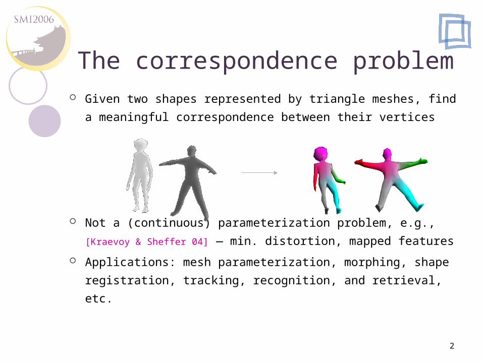
The correspondence problem Given two shapes represented by triangle meshes, find

a meaningful correspondence between their vertices

Not a (continuous) parameterization problem, e.g.,

[Kraevoy & Sheffer 04] ― min. distortion, mapped features

Applications: mesh parameterization, morphing, shape

registration, tracking, recognition, and retrieval, etc.

3

Background

A classical problem studied in computer vision mostly

We are interested in fully automatic and purely shape-

based approaches, i.e., without using prior knowledge

Goals: Invariance to common rigid and non-rigid transformation

Robustness against noise, different object size, etc.

Ultimately, return meaningful correspondences

Despite intense studies, all proposed methods can fail

on seemingly easy cases for humans

4

Two basic types of techniques

Extrinsic methods Point coordinates defined in

some global frame Optimization-based and

mostly iterative, e.g., iterative closest point (ICP)

Initial alignment is crucial

Intrinsic methods Point coordinates based on relative information A descriptor defined from the perspective of that point Descriptors can be absolute coordinates, e.g., spectral, or

statistical, e.g., shape contexts [Belongie et al. 02]

Non-rigid ICP [Chui et al. 2004]

rota

tion

5

Related works With the aid of initial manual feature correspondence

Cross parameterization [Praun et al. 01, Kraevoy & Sheffer 04]

Feature-guided ICP [Sumner & Popovic 04]

Barycentric interpolation between features [Zayer et al. 05]

Other deformation based approaches

Automatic extrinsic methods: ICP and its variants

Original ICP [Besl & McKay 92]

Many variants of rigid ICP [Rusinkiewicz & Levoy 01]

Robust ICP based on refinement [Zinber et al. 03] Non-rigid ICP based on thin-plate splines [Chui et al. 03]

6

Related works Local shape descriptors

Shape context [Belongie et al. 02, Körtgen et al. 03]

Spin images [Johnson & Hebert 99]

Other approaches that handle rigid transformations [Gelfand et al. 05, Li & Guskov 05]

Curvature map [Gatzke et al. SMI 05]

Spectral methods Original work on correspondence [Shapiro & Brady 92]

MDS for retrieval of isometric shapes [Elad & Kimmel 03]

Others: compression [Karni & Gotsman 00], spherical parameterization [Gotsman et al. 03], mesh sequencing [Isenberg & Lindstrom 05, Liu et al. 06], segmentation [Liu &

Zhang 04], surface reconstruction [Kolluri et al. 04]

7

Spectral correspondence

[Shapiro & Brady, 92]: Given two point sets P and Q Construct symmetric “affinity” matrices AP and AQ using

pair-wise L2 distances and a Gaussian kernel

Construct spectral embedding by k leading eigenvectors of AP and AQ, sorted by descending eigenvalues

Compute best matching using embedded coordinates via

L2 distance in the k-dimensional spectral domain

Why spectral correspondence? Affinities are intrinsic measure (but high-dimensional)

Eigenvectors have good approximation properties

Spectral embeddings normalize shapes with respect to all rigid body transformations and uniform scaling

8

Key observations

Flexibility of affinity measures

Whichever transformation one needs the correspondence

to be invariant of, build that invariance into affinities

Eigenvectors need to be scaled properly, e.g., at least

to handle data with difference sizes

Eigenvectors can “switch” (never reported before)

Signs of eigenvectors need to be consistent

Non-rigid shape transformation can cause non-rigid

transformation in the spectral domain

9

Summary of our approach

Use geodesic affinities for invariance to shape bending

Eigenvector scaling using squared root of eigenvalues

Proper handling of objects with difference sizes

Eigenvalue decay leaves approach less sensitive to k

Variance-normalization + interpretation from kernel PCA

Heuristics to resolve eigenvector switch and sign flip

Non-rigid ICP via thin-plate splines in spectral domain

Net result:

Proper correspondence of articulated shapes

Consistently more robust correspondence results

10

Evaluation paradigm

Visual examination via color plots Manually color one model based on parts Color second model using computed correspondence

Plot of percentage of correct matches Manually provided ground truth (small feature sets) Ground truth automatically identified via “in-place”

mesh decimation

Plot of correspondence error Sum of correspondence errors at the vertices Error at a vertex: geodesic distance between ground

truth and computed corresponding point

11

Basic steps of our algorithm

Eigenvector scaling

Non-rigid ICP via thin-plate splines

Geodesic-based

spectral embedding

Best

matching

12

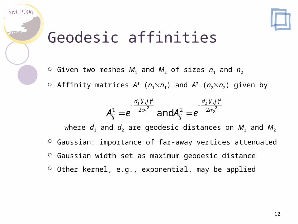
Geodesic affinities

Given two meshes M1 and M2 of sizes n1 and n2

Affinity matrices A1 (n1n1) and A2 (n2n2) given by

where d1 and d2 are geodesic distances on M1 and M2

Gaussian: importance of far-away vertices attenuated

Gaussian width set as maximum geodesic distance

Other kernel, e.g., exponential, may be applied

22

22

21

21

2

),(

22

),(

1 and jid

ij

jid

ij eAeA

13

Spectral embeddings

Eigen-decompose each affinity matrix A = UUT

Obtain k-D spectral embedding of mesh vertices

using the k leading (scaled) eigenvectors of A

First eigenvector ignored as it is almost a constant

k

uuu

ikii

k

kk

uuu

E

21

2211

k-dimensional spectral embedding coordinates of ith the point of mesh

14

Examples: 3D spectral embeddings

Use of 2nd, 3rd, and 4th scaled eigenvectors

15

Eigenvector scaling

EkEkT gives the best rank-k approximation of the

affinity matrix A (namely, dot product affinity)

Scaling using the square root of the eigenvalues is

shown to normalize the

variance of data

The scaling is also a

natural one when seen

from the perspective of

kernel PCA [Jain 2006]

16

Eigenvector switching and sign flips

Signs of the eigenvectors are decided by eigensolver

and are difficult to correspond automatically

Discrepancy between shapes can also cause certain

eigenvectors to switch places

An eigenvector switch or a sign flip corresponds to a

reflection in the spectral domain

17

Exhaustive search and greedy heuristic

Reflection-invariant shape descriptors possible, e.g.,

high-D shape context or symmetric polynomials, but

more invariance less descriptivity [Frome et al. 04]

Choose among 2kk! possible eigenvector ordering and

sign flips to minimize a correspondence cost:

Besides exhaustive search (for very small k), can use

greedy scheme to order one eigenvector at a time

1

1

22

)(1 ˆˆ

n

iiCi EE

18

Non-rigid transformations

Perform non-rigid ICP using thin-plate splines in the spectral domain

Experimentally, very fast convergence (5-10 iterations)

19

Recap of algorithm

Eigenvector scaling

Non-rigid ICP via thin-plate splines

Geodesic-based

spectral embedding

Best

matching

20

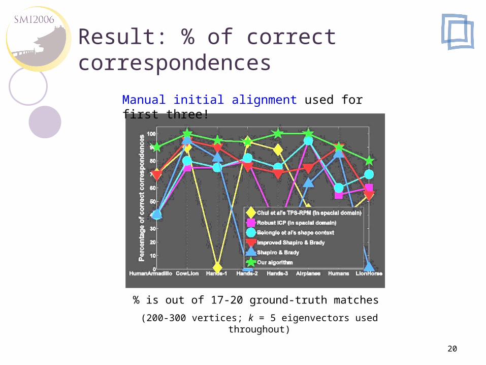
Result: % of correct correspondences

Manual initial alignment used for first three!

% is out of 17-20 ground-truth matches

(200-300 vertices; k = 5 eigenvectors used throughout)

21

Visual results for correspondence

Models with articulation and moderate stretching

Many more results in color plate (page 300).

22

Limitations Intrinsic geodesic affinities

Symmetry issue

Topological issue: hybrid approach [Jain & Zhang 06]

Rather primitive heuristic for resolving eigenvector

switching and sign flips Effectiveness attributed to spectral normalization

Euclidean metric as correspondence cost No particular reason, except for a computational one

Challenge: what is right?

Computational complexity: O(n2logn)

23

Follow-up and future works Sampling via Nyström approximation [Liu et al. 06]

Spectral embedding: O(n2logn) O(pnlogn + p3)

Little loss of quality at low sampling (10 out of 4000)

Farthest point sampling used

More sophisticated sampling schemes [Liu & Zhang 06]

Retrieval of articulated shapes [Jain & Zhang 06]

Outperforms light-field descriptor [Chen et al. 03] and spherical Harmonics descriptor [Kazhdan et al. 03] (even when these are applied to spectral embeddings)

But not so on Princeton Benchmark database (yet) due to various artifacts in the models

How about eigenspaces?

24

Acknowledgement

NSERC Grant 611370

MITACS Grant on project: Mathematical Surface

Representations for Conceptual Design

MATLAB code of non-rigid ICP [Chui et al. 03]

Greg Mori for helpful discussions

Reviewers’ comments and for pointing out a couple

of missing references

Thank you!