Embed Size (px)
Citation preview

. . . . . .
ROBOTICS: ADVANCED CONCEPTS
&ANALYSIS
MODULE 2 – ELEMENTS OF ROBOTS: JOINTS, LINKS,ACTUATORS & SENSORS
Ashitava Ghosal1
1Department of Mechanical Engineering&
Centre for Product Design and ManufactureIndian Institute of ScienceBangalore 560 012, India
Email: [email protected]
NPTEL, 2010
ASHITAVA GHOSAL (IISC) ROBOTICS: ADVANCED CONCEPTS & ANALYSIS NPTEL, 2010 1 / 138

. . . . . .
.. .1 CONTENTS
.. .2 LECTURE 1Mathematical PreliminariesHomogeneous Transformation
.. .3 LECTURE 2Elements of a robot – JointsElements of a robot – Links
.. .4 LECTURE 3Examples of D-H Parameters & Link TransformationMatrices
.. .5 LECTURE 4Elements of a robot – Actuators & Transmission
.. .6 LECTURE 5Elements of a robot – Sensors
.. .7 ADDITIONAL MATERIALProblems, References, and Suggested Reading
ASHITAVA GHOSAL (IISC) ROBOTICS: ADVANCED CONCEPTS & ANALYSIS NPTEL, 2010 2 / 138

. . . . . .
OUTLINE.. .1 CONTENTS.. .2 LECTURE 1
Mathematical PreliminariesHomogeneous Transformation
.. .3 LECTURE 2Elements of a robot – JointsElements of a robot – Links
.. .4 LECTURE 3Examples of D-H Parameters & Link TransformationMatrices
.. .5 LECTURE 4Elements of a robot – Actuators & Transmission
.. .6 LECTURE 5Elements of a robot – Sensors
.. .7 ADDITIONAL MATERIALProblems, References, and Suggested Reading
ASHITAVA GHOSAL (IISC) ROBOTICS: ADVANCED CONCEPTS & ANALYSIS NPTEL, 2010 3 / 138

. . . . . .
POSITION OF A RIGID BODY
Rigid Body A
{A}
XA
YAOA
Ap
ZA
Figure 1: Position of point Pdenoted by Ap
Position of a point of interestsuch as centre ofmass/gravity.Right-handed coordinatesystem specified by
Origin OA.Set of 3 mutuallyorthogonal axis —Unitvectors XA, YA and ZAare along the index finger,the middle finger and thethumb of the right-hand,respectively.Label to keep track — {A}.
Point Ap with Cartesian coordinates (px ,py ,pz)T
Ap = px XA+py YA+pz ZA = (px ,py ,pz)T (1)
ASHITAVA GHOSAL (IISC) ROBOTICS: ADVANCED CONCEPTS & ANALYSIS NPTEL, 2010 4 / 138

. . . . . .
ORIENTATION OF A RIGID BODY
Position of one point on the rigid body not enough todescribe it in 3D space.Orientation of a rigid body B with respect to {A}
YA
YB
Bp
Rigid Body B
ϕ
kZA
XB
{B}
{A}
ZB
OA,OB
XA
Figure 2: Orientation of a rigid body
Attach coordinatesystem, {B}, to rigidbody B .Origin of {B}coincident with origin of{A} (see Figure 2).Obtain description of{B} with respect to{A}.
ASHITAVA GHOSAL (IISC) ROBOTICS: ADVANCED CONCEPTS & ANALYSIS NPTEL, 2010 5 / 138

. . . . . .
ORIENTATION – DIRECTION COSINES
Unit vectors XB , YB , and ZB , attached to B , can bedescribed in {A}
AXB = r11XA+ r21YA+ r31ZAAYB = r12XA+ r22YA+ r32ZA (2)AZB = r13XA+ r23YA+ r33ZA
rij , i , j = 1,2,3 are called direction cosinesr11 =
A XB · XAMagnitude of unit vectors are 1 → r11 is cosine of anglebetween AXB and XA. All rij ’s are cosines of angles.
Define 3×3 rotation matrix AB [R] with rij , i , j = 1,2,3 as
its elements. Columns of AB [R] are AXB , AYB , and AZB .
AB [R] completely describes all three coordinate axis of {B}with respect to {A}.AB [R] gives orientation of rigid body B in {A}.
ASHITAVA GHOSAL (IISC) ROBOTICS: ADVANCED CONCEPTS & ANALYSIS NPTEL, 2010 6 / 138
. . . . . .
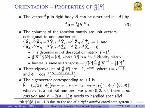
ORIENTATION – PROPERTIES OF AB [R]
The vector Bp in rigid body B can be described in {A} byAp = A
B [R]Bp (3)
The columns of the rotation matrix are unit vectors,orthogonal to one another ⇒AXB ·A XB =A YB ·A YB =A ZB ·A ZB = 1, andAXB ·A YB =A YB ·A ZB =A ZB ·A XB = 0
The determinant of the rotation matrix is +11.AB [R]
T AB [R] = [U], where [U] is a 3×3 identity matrix.
Inverse is same as transpose — BA [R]
∆= A
B [R]−1
= AB [R]
T .Three eigenvalues of A
B [R] are +1, e±ıϕ , where ı =√−1,
and ϕ = cos−1( r11+r22+r33−12 ).
The eigenvector corresponding to +1 isk = (1/2sinϕ)[r32− r23, r13− r31, r21− r12]
T , ϕ = {0,nπ},where n is a natural number. For ϕ = {0,2nπ}, there is norotation and ϕ = 2(n−1)π needs to handled specially!
1det(AB [R]) = +1 is due to the use of a right-handed coordinate system.ASHITAVA GHOSAL (IISC) ROBOTICS: ADVANCED CONCEPTS & ANALYSIS NPTEL, 2010 7 / 138
. . . . . .
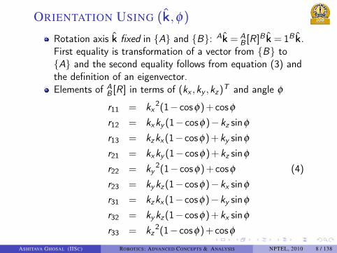
ORIENTATION USING (k,ϕ)Rotation axis k fixed in {A} and {B}: Ak = A
B [R]B k = 1B k.First equality is transformation of a vector from {B} to{A} and the second equality follows from equation (3) andthe definition of an eigenvector.Elements of A
B [R] in terms of (kx ,ky ,kz)T and angle ϕ
r11 = kx2(1− cosϕ)+ cosϕ
r12 = kxky (1− cosϕ)−kz sinϕr13 = kzkx(1− cosϕ)+ky sinϕr21 = kxky (1− cosϕ)+kz sinϕr22 = ky
2(1− cosϕ)+ cosϕ (4)r23 = kykz(1− cosϕ)−kx sinϕr31 = kzkx(1− cosϕ)−ky sinϕr32 = kykz(1− cosϕ)+kx sinϕr33 = kz
2(1− cosϕ)+ cosϕ
ASHITAVA GHOSAL (IISC) ROBOTICS: ADVANCED CONCEPTS & ANALYSIS NPTEL, 2010 8 / 138

. . . . . .
ORIENTATION – SIMPLE ROTATION
Rotation axis k is parallel to XA and hence to XB →Rotation about X axis.
AB [R] = [R(X,ϕ)] =
1 0 00 cosϕ −sinϕ0 sinϕ cosϕ
(5)
ZA
Bp
Rigid Body BXA, XB
kϕ
ϕ
{B}
{A}
ZB
OA, OB YA
YB
Figure 3: Rotation about X by angle ϕ
Rotation about Xshown in Figure 3.
ASHITAVA GHOSAL (IISC) ROBOTICS: ADVANCED CONCEPTS & ANALYSIS NPTEL, 2010 9 / 138

. . . . . .
SIMPLE ROTATIONS (CONTD.)
Rotation about Y and Z
[R(Y,ϕ)] =
cosϕ 0 sinϕ0 1 0
−sinϕ 0 cosϕ
(6)
[R(Z,ϕ)] =
cosϕ −sinϕ 0sinϕ cosϕ 0
0 0 1
(7)
Rotation matrices in equations (5) through (7) calledsimple rotations.
ASHITAVA GHOSAL (IISC) ROBOTICS: ADVANCED CONCEPTS & ANALYSIS NPTEL, 2010 10 / 138

. . . . . .
SUCCESSIVE ROTATIONS
Two successive rotations:...1 Initially B is coincident with {A}....2 First rotation relative to {A}. After first rotation{A}→ {B1}.
...3 Second rotation relative to {B1}. After second rotation{B1}→ {B}.
{B}
{A}
ZB
ZA
YA
YB
Rigid Body BXA
XB1
XB
YB1
ZB1
OA,OB1,OB
Rigid Body B1
Figure 4: Successive rotation
Resultant rotation:AB [R] = A
B1[R] B1
B [R] — Note orderof matrix multiplication.Resultant of n rotations —AB [R] = A
B1[R] B1
B2[R] ... Bn−1
B [R]
Matrix multiplication is noncommutative in general —AB1[R] B1
B [R] = B1B [R] A
B1[R]
⇒ Order of rotation is important!
ASHITAVA GHOSAL (IISC) ROBOTICS: ADVANCED CONCEPTS & ANALYSIS NPTEL, 2010 11 / 138

. . . . . .
ORIENTATION – THREE ANGLES
Orientation described by 3 independent parameters →Three rotations completely describe orientation of a rigidbody.Three successive rotations about axes fixed to moving body
Rotations about three distinct axes: 6 combinations –X-Y-Z, X-Z-Y, Y-Z-X, Y-X-Z, Z-X-Y & Z-Y-XRotations about two distinct axes: 6 combinations –X-Y-X, X-Z-X, Y-X-Y, Y-Z-Y, Z-X-Z, & Z-Y-Z
Rotations about axes fixed in space – 12 possiblecombinations for 3 and 2 distinct axes.Minimal representation of orientation of rigid body – Onlythree parameters (angles) and no constraints.Three angles also called Euler angles.
ASHITAVA GHOSAL (IISC) ROBOTICS: ADVANCED CONCEPTS & ANALYSIS NPTEL, 2010 12 / 138

. . . . . .
X–Y–Z EULER ANGLES
Rotation about X – AB1
[R] = [R(X,θ1)] =
1 0 00 cosθ1 −sinθ10 sinθ1 cosθ1
Rotation about Y – B1
B2[R] = [R(Y,θ2)] =
cosθ2 0 sinθ20 1 0
−sinθ2 0 cosθ2
XA, XB1
YA
YB1
ZA
ZB1
XA, XB1
YA θ2
ZA
ZB1
ZB2
XA, XB1
{B2}
{A}, {B1}
ZA
YA
YB1
YB
ZB, ZB2
XB2
XB2
{B}
OA, OB OA, OB
θ3
XB
{B2}
YB1, YB2
ZB1
{A}{B1}
θ1
OA, OB
{A}, {B1}
Figure 5: X–Y–Z Euler angles
ASHITAVA GHOSAL (IISC) ROBOTICS: ADVANCED CONCEPTS & ANALYSIS NPTEL, 2010 13 / 138
. . . . . .
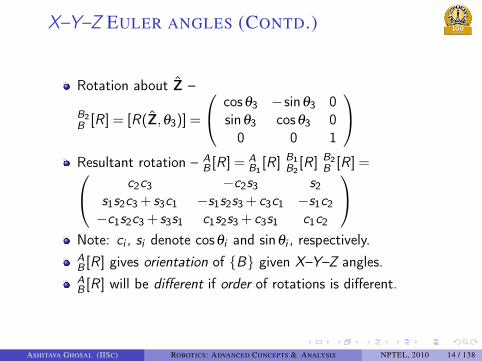
X–Y–Z EULER ANGLES (CONTD.)
Rotation about Z –
B2B [R] = [R(Z,θ3)] =
cosθ3 −sinθ3 0sinθ3 cosθ3 0
0 0 1
Resultant rotation – A
B [R] = AB1[R] B1
B2[R] B2
B [R] = c2c3 −c2s3 s2s1s2c3+ s3c1 −s1s2s3+ c3c1 −s1c2−c1s2c3+ s3s1 c1s2s3+ c3s1 c1c2
Note: ci , si denote cosθi and sinθi , respectively.AB [R] gives orientation of {B} given X–Y–Z angles.AB [R] will be different if order of rotations is different.
ASHITAVA GHOSAL (IISC) ROBOTICS: ADVANCED CONCEPTS & ANALYSIS NPTEL, 2010 14 / 138
. . . . . .
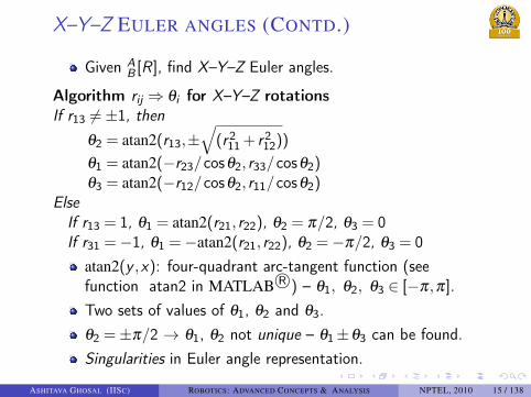
X–Y–Z EULER ANGLES (CONTD.)
Given AB [R], find X–Y–Z Euler angles.
Algorithm rij ⇒ θi for X–Y–Z rotationsIf r13 =±1, then
θ2 = atan2(r13,±√
(r211+ r2
12))
θ1 = atan2(−r23/cosθ2, r33/cosθ2)θ3 = atan2(−r12/cosθ2, r11/cosθ2)
ElseIf r13 = 1, θ1 = atan2(r21, r22), θ2 = π/2, θ3 = 0If r31 =−1, θ1 =−atan2(r21, r22), θ2 =−π/2, θ3 = 0
atan2(y ,x): four-quadrant arc-tangent function (seefunction atan2 in MATLAB R⃝) – θ1, θ2, θ3 ∈ [−π,π].Two sets of values of θ1, θ2 and θ3.θ2 =±π/2 → θ1, θ2 not unique – θ1±θ3 can be found.Singularities in Euler angle representation.
ASHITAVA GHOSAL (IISC) ROBOTICS: ADVANCED CONCEPTS & ANALYSIS NPTEL, 2010 15 / 138

. . . . . .
Z–Y–Z EULER ANGLES
OA, OB OA, OB
ZA, ZB1ZA, ZB1
YB1, YB2
XB1
XB2
XB
{A}{B1}
θ1
ZA, ZB1
XA
XB1
YA
YB1
OA, OB
{B2}{A}, {B1}
θ2
XA
XB1 XB2
YA
YB1, YB2
ZB2
θ3
ZB2, ZB
XA
YA
YB
{A}{B}
Figure 6: Z–Y–Z Euler angles
AB [R] =
c1 −s1 0s1 c1 00 0 1
c2 0 s20 1 0
−s2 0 c2
c3 −s3 0s3 c3 00 0 1
=
c1c2c3− s1s3 −c1c2s3− s1c3 c1s2s1c2c3+ c1s3 −s1c2s3+ c1c3 s1s2
−s2c3 s2s3 c2
(8)
ASHITAVA GHOSAL (IISC) ROBOTICS: ADVANCED CONCEPTS & ANALYSIS NPTEL, 2010 16 / 138

. . . . . .
Z–Y–Z EULER ANGLES (CONTD.)
Algorithm rij ⇒ Z–Y–Z Euler anglesIf r33 =±1, then
θ2 = atan2(±√
(r231+ r2
32), r33)
θ1 = atan2(r23/sinθ2, r13/sinθ2)θ3 = atan2(r32/sinθ2,−r31/sinθ2)
ElseIf r33 = 1, then
θ1 = θ2 = 0, θ3 = atan2(−r12, r11)If r33 =−1, then
θ1 = 0, θ2 = π, θ3 = atan2(r12,−r11)
Two possible sets of Z–Y–Z Euler angles (θ1,θ2,θ3) for agiven A
B [R].r33 =±1 → Singularity → θ1±θ3 can be found.For unique θ1 and θ3 when r33 =±1 → Choose θ1 = 0.
ASHITAVA GHOSAL (IISC) ROBOTICS: ADVANCED CONCEPTS & ANALYSIS NPTEL, 2010 17 / 138

. . . . . .
OTHER REPRESENTATIONS
Euler parameters (see Kane et al., 1983, McCarthy, 1990):4 parameters derived from k = (kx ,ky ,kz)
T and angle ϕ3 parameters — ε = k sinϕ/2fourth parameter — ε4 = cosϕ/2One constraint — ε1
2+ ε22+ ε3
2+ ε42 = 1
Quaternions (pp. 185 Arfken(1985), Wolfram website2): 4parameters
‘Sum’ of a scalar q0 and a vector (q1,q2,q3)T —
Q = q0+q1i+q2 j+q3k.i, j, and k are the unit vectors in ℜ3.Product of two quaternion also a quaternion.Inverse of quaternion exists.q20 +q2
1 +q22 +q2
3 = 1 → Unit quaternion representorientation of a rigid body in ℜ3.
2See Known Bugs in Module 0, slide #10 for viewing links.ASHITAVA GHOSAL (IISC) ROBOTICS: ADVANCED CONCEPTS & ANALYSIS NPTEL, 2010 18 / 138

. . . . . .
ORIENTATION OF A RIGID BODY –SUMMARY
Orientation of a rigid body in ℜ3 is specified by 3independent parameters.Various representation of orientation with their ownadvantages and disadvantages
Rotation matrix AB [R] – 9 rij ’s + 6 constraints → Too
many variables and constraints but ideal for analysis.Axis (kx ,ky ,kz)
T and angle ϕ – 4 parameters + oneconstraint k2
x +k2y +k2
z = 1 → Useful for insight andextension to screws, twists and wrenches.Euler angles: 3 parameters and zero constraints→ Minimalrepresentation but suffer from problem of singularities andsequence must be known.Euler parameters and quaternions: 4 parameters +1constraint → Similar but not exactly same as axis-angleform, no singularities, used in motion planning.
Can convert from one representation to any other forregular cases!
ASHITAVA GHOSAL (IISC) ROBOTICS: ADVANCED CONCEPTS & ANALYSIS NPTEL, 2010 19 / 138

. . . . . .
COMBINED TRANSLATION AND
ORIENTATION OF A RIGID BODY
{A}
OA
OB
ApAOB
Bp
Rigid Body B
XA
{B}
YA
ZA
XB
YB
ZB
Figure 7: General transformation
{A} and {B}, OA andOB not coincidentOrientation of {B} withrespect to {A} – A
B [R]Ap =A OB +A
B [R]BpAOB locates OB withrespect to OA.
ASHITAVA GHOSAL (IISC) ROBOTICS: ADVANCED CONCEPTS & ANALYSIS NPTEL, 2010 20 / 138

. . . . . .
OUTLINE.. .1 CONTENTS.. .2 LECTURE 1
Mathematical PreliminariesHomogeneous Transformation
.. .3 LECTURE 2Elements of a robot – JointsElements of a robot – Links
.. .4 LECTURE 3Examples of D-H Parameters & Link TransformationMatrices
.. .5 LECTURE 4Elements of a robot – Actuators & Transmission
.. .6 LECTURE 5Elements of a robot – Sensors
.. .7 ADDITIONAL MATERIALProblems, References, and Suggested Reading
ASHITAVA GHOSAL (IISC) ROBOTICS: ADVANCED CONCEPTS & ANALYSIS NPTEL, 2010 21 / 138

. . . . . .
4×4 TRANSFORMATION MATRIX
Combined translation and orientation AP = AB [T ]BP
AP and BP are 4×1 homogeneous coordinates (seeAdditional Material) constructed by concatenating a ‘1’ toAp and BpAP = [Ap | 1]T and BP = [Bp | 1]T
4×4 homogeneous transformation matrix AB [T ] is formed as
AB [T ] =
( AB [R] AOB
0 0 0 1
)(9)
In computer graphics and computer vision → Last row isused for perspective and scaling and not [0 0 0 1].Upper left 3×3 matrix is identity matrix → Puretranslation.Top right 3×1 vector is zero → Pure rotation.
ASHITAVA GHOSAL (IISC) ROBOTICS: ADVANCED CONCEPTS & ANALYSIS NPTEL, 2010 22 / 138
. . . . . .
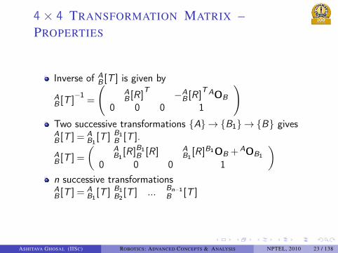
4 × 4 TRANSFORMATION MATRIX –PROPERTIES
Inverse of AB [T ] is given by
AB [T ]
−1=
(AB [R]
T −AB [R]
T AOB0 0 0 1
)Two successive transformations {A}→ {B1}→ {B} givesAB [T ] = A
B1[T ] B1
B [T ].
AB [T ] =
( AB1[R]B1
B [R] AB1[R]B1OB +AOB1
0 0 0 1
)n successive transformationsAB [T ] = A
B1[T ] B1
B2[T ] ... Bn−1
B [T ]
ASHITAVA GHOSAL (IISC) ROBOTICS: ADVANCED CONCEPTS & ANALYSIS NPTEL, 2010 23 / 138

. . . . . .
PROPERTIES OF AB [T ] (CONTD.)
Four eigenvalues of AB [T ] are +1, +1,e±ıϕ , ϕ same as for
AB [R].Eigenvectors for +1 is k – No other eigenvector!AB [T ] represents the general motion of a rigid body in 3Dspace → 6 parameters must be present.General motion of rigid body as a twist – Rotation abouta line and translation along the line.
Direction of the line: (kx ,ky ,kz)T → 2 independent
parameters.Rotation about the line: angle ϕ → 1 independentparameter.Location of the line in ℜ3: (k,Y× k) where
Y =([U]−A
B [R]T)AOB
2(1−cosϕ)
→ 4 independent parameters in k and Y× k.Translation along the line by an amount (AOB · k).
More details about twists, eigenvalues and eigenvectors(see Sangamesh Deepak and Ghosal, 2006).
ASHITAVA GHOSAL (IISC) ROBOTICS: ADVANCED CONCEPTS & ANALYSIS NPTEL, 2010 24 / 138

. . . . . .
SUMMARY
A rigid body B in 3D space has 6 DOF with respect toanother rigid body A: 3 for position & 3 for orientation.Definition of a right-handed coordinate system {A} → X,Y, Z and origin OA.Rigid body B conceptually identical to a coordinate system{B}.Position of rigid body → Position of a point of interest onrigid body with respect to coordinate system {A} → 3Cartesian coordinates: Ap = (px ,py ,pz)
T .Orientation described in many ways: 1) by 3×3 rotationmatrix A
B [R], 2) (ϕ , k) or angle-axis form, 3) 3 Eulerangles, 4) Euler parameters & quaternions.Algorithms available to convert one representation toanother.4×4 homogeneous transformation matrix, A
B [T ], representposition and orientation in a compact manner.Properties of A
B [T ] can be related to a screw.ASHITAVA GHOSAL (IISC) ROBOTICS: ADVANCED CONCEPTS & ANALYSIS NPTEL, 2010 25 / 138

. . . . . .
OUTLINE.. .1 CONTENTS.. .2 LECTURE 1
Mathematical PreliminariesHomogeneous Transformation
.. .3 LECTURE 2Elements of a robot – JointsElements of a robot – Links
.. .4 LECTURE 3Examples of D-H Parameters & Link TransformationMatrices
.. .5 LECTURE 4Elements of a robot – Actuators & Transmission
.. .6 LECTURE 5Elements of a robot – Sensors
.. .7 ADDITIONAL MATERIALProblems, References, and Suggested Reading
ASHITAVA GHOSAL (IISC) ROBOTICS: ADVANCED CONCEPTS & ANALYSIS NPTEL, 2010 26 / 138

. . . . . .
JOINTS – INTRODUCTION
A joint connects two or more links.A joint imposes constraints on the links it connects.
2 free rigid bodies have 6+6 degrees of freedom.Hinge joint connecting two free rigid bodies → 6+1degrees of freedom.Hinge joint imposes 5 constraints, i.e., hinge joint allows 1relative (rotary) degree of freedom.
Degree of freedom of a joint in 3D space: 6−m where m isthe number of constraint imposed.Serial manipulators → All joints actuated →One-degree-of-freedom joints used.Parallel and hybrid manipulators → Some joints passive →Multi-degree-of-freedom joints can be used.
ASHITAVA GHOSAL (IISC) ROBOTICS: ADVANCED CONCEPTS & ANALYSIS NPTEL, 2010 27 / 138

. . . . . .
TYPES OF JOINTSD O F
Figure 8: – Types of joints
ASHITAVA GHOSAL (IISC) ROBOTICS: ADVANCED CONCEPTS & ANALYSIS NPTEL, 2010 28 / 138

. . . . . .
CONSTRAINTS IMPOSED BY A
ROTARY (R) JOINT∗Rigid bodies, {i −1} and{i}, connected by a rotary(R) joint (Figure 9).{i} can rotate about k,with respect to {i −1}, byangle θi0i [R] = 0
i−1[R] i−1i [R(k,θi )]
Three independentequations in the matrixequation above; θi isunknown⇒ 2 constraintsin the 3 equations.
{0}
{i − 1}
{i}
Oi−1
Oi
ip
i−1p
0Oi−1
0Oi
0p
k
Li
θiRigid Body i − 1
Rigid Body i
Rotary Joint
Figure 9: A rotary joint
For a common point P on the rotation axis along line Li0p =0 Oi−1+
0i−1[R]i−1p =0 Oi +
0i [R]ip ⇒ 3 constraints
present.ASHITAVA GHOSAL (IISC) ROBOTICS: ADVANCED CONCEPTS & ANALYSIS NPTEL, 2010 29 / 138
. . . . . .
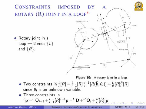
CONSTRAINTS IMPOSED BY A
ROTARY (R) JOINT IN A LOOP∗
Rotary joint in aloop — 2 ends {L}and {R}.
k
Li
θi
Rotary Joint
Rigid Body i − 1
Oi−1
Oi
{L}
LOi−1
i−1p
ip
{R}
Rigid Body i
ROi
LD
{i − 1}
{i}
Figure 10: A rotary joint in a loop
Two constraints in Li [R] = L
i−1[R] i−1i [R(k,θi )] =
LR [R]Ri [R]
since θi is an unknown variable.Three constraints inLp =L Oi−1+
Li−1[R]i−1p =L D+R Oi +
Ri [R]ip
ASHITAVA GHOSAL (IISC) ROBOTICS: ADVANCED CONCEPTS & ANALYSIS NPTEL, 2010 30 / 138

. . . . . .
CONSTRAINTS IMPOSED BY A
PRISMATIC (P) JOINT∗Two rigid bodies,{i −1} and {i},connected by asliding/prismatic (P)jointOrientation of {i} issame as {i −1} ⇒ 3independent constraintsin 0
i [R] = 0i−1[R]
{i} can slide by di ,along Li , with respectto {i −1}
{0}
k
Li
di
Rigid Body i − 1
Rigid Body i
{i − 1}
{i}
Oi−1
Oi
0Oi−1
i−1p
ip
0Oi Prismatic Joint0p
Figure 11: A prismatic joint
2 constraints in 0Oi−1+0i−1[R]i−1p+di k =0 Oi +
0i [R]ip
since di is an unknown variable.ASHITAVA GHOSAL (IISC) ROBOTICS: ADVANCED CONCEPTS & ANALYSIS NPTEL, 2010 31 / 138

. . . . . .
CONSTRAINTS IMPOSED BY A
SPHERICAL (S) JOINT∗
Spherical(S) or ball andsocket joint allows threerotations.S joint can berepresented as 3intersecting rotary(R)joints. {0}
Rigid Body i − 1
Rigid Body i
{i}
{i − 1}
0Oi−1
0Oi
Spherical Joint
i−1p
ip
0p
Figure 12: A spherical joint
3 constraints: 0p =0 Oi−1+0i−1[R]i−1p =0 Oi +
0i [R]ip
ASHITAVA GHOSAL (IISC) ROBOTICS: ADVANCED CONCEPTS & ANALYSIS NPTEL, 2010 32 / 138

. . . . . .
CONSTRAINTS IMPOSED BY A
HOOKE (U) JOINT∗
Common in many parallel manipulators.Equivalent to two intersecting rotary (R) joints → Twodegrees of freedom → 4 constraints.For a common point P at the intersection of two rotationaxes 0p =0 Oi−1+
0i−1[R]i−1p =0 Oi +
0i [R]ip → 3
constraints.0i [R] = 0
i−1[R] i−1i [R(k1,θ1i )][R(k2,θ2i )] → Only 1
constraint present as θ1i and θ2i are unknown rotationsabout k1 and k2
ASHITAVA GHOSAL (IISC) ROBOTICS: ADVANCED CONCEPTS & ANALYSIS NPTEL, 2010 33 / 138

. . . . . .
CONSTRAINTS IMPOSED BY A
SPHERICAL-SPHERICAL (S–S) JOINT
PAIR
The S–S pair appearin many parallelmanipulators.Distance betweentwo spherical joint isconstant. {L}
Rigid Body i
Si
{i}
LSiL
Oi
iSi
{j}
Sj
jSj
RO
RSj
lij
Rigid Body j
S-S Pair
LD
Figure 13: A S–S pair in a loop
One constraint equation(LSi − (LD+R Sj)) · (LSi − (LD+R Sj)) = l2ij , lij is aconstant.
ASHITAVA GHOSAL (IISC) ROBOTICS: ADVANCED CONCEPTS & ANALYSIS NPTEL, 2010 34 / 138

. . . . . .
OUTLINE.. .1 CONTENTS.. .2 LECTURE 1
Mathematical PreliminariesHomogeneous Transformation
.. .3 LECTURE 2Elements of a robot – JointsElements of a robot – Links
.. .4 LECTURE 3Examples of D-H Parameters & Link TransformationMatrices
.. .5 LECTURE 4Elements of a robot – Actuators & Transmission
.. .6 LECTURE 5Elements of a robot – Sensors
.. .7 ADDITIONAL MATERIALProblems, References, and Suggested Reading
ASHITAVA GHOSAL (IISC) ROBOTICS: ADVANCED CONCEPTS & ANALYSIS NPTEL, 2010 35 / 138

. . . . . .
LINKS – INTRODUCTION
A link A is a rigid body in 3D space → Can be describedby a coordinate system {A}.A rigid body in ℜ3 has 6 degrees of freedom → 3 rotation+ 3 translation → 6 parameters (see Lecture 1)For links connected by rotary (R) and prismatic (P),possible to use 4 parameters – Denavit-Hartenberg(D-H)parameters (see Denavit & Hartenberg, 1955).4 parameters since lines related to rotary(R) and prismatic(P) joint axis are used.For multi-degree-of-freedom joints → Use equivalentnumber of one-degree-of-freedom joints.
ASHITAVA GHOSAL (IISC) ROBOTICS: ADVANCED CONCEPTS & ANALYSIS NPTEL, 2010 36 / 138

. . . . . .
LINKS – DENAVIT-HARTENBERG
(D-H) PARAMETERS
A word about conventions – Several ways to derive D-Hparameters!Convention used:
...1 Coordinate system {i} is attached to the link i .
...2 Origin of {i} lies on the joint axis i – Link i is “after” jointi .
...3 “after” for serial manipulators – Numbers increasing fromfixed {0} → Link 1 {1} → . . . → Free end {n}.
...4 “after” for parallel manipulators – Not so straight-forwarddue to one or more loops.
Convention same as in Craig (1986) or Ghosal(2006).
ASHITAVA GHOSAL (IISC) ROBOTICS: ADVANCED CONCEPTS & ANALYSIS NPTEL, 2010 37 / 138

. . . . . .
ASSIGNMENT OF COORDINATE AXES
Three intermediate links — {i −1}, {i} and {i +1}.Rotary joint axis — Labeled Zi−1, Zi and Zi+1 .
{0}
X0
Y0
Z0
Zi+1
Oi−1
Oi
{i − 1}
{i}
Xi−1
X
Link i − 2
Link i − 1
Link i
Link i + 1
Li−1
Li
Li+1
ZiZi−1
ai−1
di
θi
αi−1
Figure 14: Intermediate links and D-H parameters
ASHITAVA GHOSAL (IISC) ROBOTICS: ADVANCED CONCEPTS & ANALYSIS NPTEL, 2010 38 / 138

. . . . . .
D-H PARAMETERS – ASSIGNMENT
OF COORDINATE AXIS (CONTD.)
For coordinate system {i −1}Zi−1 is along joint axis i −1.Xi−1 is chosen along the common perpendicular betweenlines Li−1 and Li .Yi−1 = Zi−1× Xi−1 – Right-handed coordinate system.The origin Oi−1 is the point of intersection of the mutualperpendicular line and the line Li−1.
For coordinate system {i}: Zi is along the joint axis i , Xiis along the common perpendicular between Zi and Zi+1,and the origin of {i}, Oi , is the point of intersection of theline along Xi and line along Zi (see Figure 14).
ASHITAVA GHOSAL (IISC) ROBOTICS: ADVANCED CONCEPTS & ANALYSIS NPTEL, 2010 39 / 138

. . . . . .
D-H PARAMETERS FOR LINK iTwist angle αi−1 — Twist angle for link i has subscripti −1!
Angle between joints axis i −1 and i & measured aboutXi−1 using right-hand rule (see Figure 14).Signed quantity between 0 and ±π radians.
Link length ai−1 — Link length for link i is ai−1!Distance between joints axis i −1 and i & measured alongXi−1 (see Figure 14).Always a positive quantity.
Link offset diMeasured along Zi from Xi−1 to Xi – Can be < 0.Joint i rotary → di constant.Joint i prismatic → di is joint variable (see Figure 14).
Rotation angle θiAngle between Xi−1 and Xi measured about Zi usingright-hand rule – Between 0 and ±π radians.Joint i is prismatic → θi is constant.Joint i rotary → θi is joint variable (see Figure 14).
ASHITAVA GHOSAL (IISC) ROBOTICS: ADVANCED CONCEPTS & ANALYSIS NPTEL, 2010 40 / 138

. . . . . .
D-H PARAMETERS – SPECIAL CASES
Consecutive joints axis parallel → ∞ commonperpendiculars
αi−1 = 0,π, ai−1 along any common perpendicular.Joint i is rotary (R) → di is taken as zero.Joint i is prismatic (P) → θi is taken as zero.Consecutive P joints parallel → d ’s not independent!
Consecutive joints axis intersecting → ai−1 = 0 and Xnormal to plane.First link {1}: choice of Z0 and thereby X1 is arbitrary.
R joint → Choose {0} and {1} coincident &αi−1 = ai−1 = 0, di = 0.P joint → Choose {0} and {1} parallel &αi−1 = ai−1 = θi = 0.
Last link {n}: Zn+1 not definedR joint → Origins of {n} and {n+1} are chosencoincident & dn = 0 and θn = 0 when Xn−1 aligns with Xn.P joint → Xn is chosen such that θn = 0 & origin On ischosen at the intersection of Xn−1 and Zn when dn = 0.
ASHITAVA GHOSAL (IISC) ROBOTICS: ADVANCED CONCEPTS & ANALYSIS NPTEL, 2010 41 / 138

. . . . . .
LINK TRANSFORMATION MATRICES
Four D-H parameters describe link i with respect to linki −1
Orientation of of {i} with respect to {i −1} is given byi−1i [R] = [R(X,αi−1)][R(Z,θi )]Location of origin of {i} with respect to {i −1} is given byi−1Oi = ai−1
i−1Xi−1+dii−1Zi
Recall i−1Xi−1 = (1,0,0)T . The vector i−1Zi is the lastcolumn of i−1
i [R] and is (0,−sαi−1 ,cαi−1)T 3.
The 4×4 transformation matrix relating {i} with respectto {i −1} is
i−1i [T ] =
cθi −sθi 0 ai−1
sθi cαi−1 cθi cαi−1 −sαi−1 −sαi−1disθi sαi−1 cθi sαi−1 cαi−1 cαi−1di
0 0 0 1
(10)
3The symbols −sαi−1 , cαi−1 denote sin(αi−1) and cos(αi−1),respectively. Please see Notations in Module 0.
ASHITAVA GHOSAL (IISC) ROBOTICS: ADVANCED CONCEPTS & ANALYSIS NPTEL, 2010 42 / 138

. . . . . .
LINK TRANSFORMATION MATRICES
i−1i [T ] is a function only one joint variable — di or θi .i−1Oi locates a point on the joint axis i at the beginning oflink i .Position and orientation of link i determined by αi−1 andai−1. Note: subscript i −1 in the twist angle and length!The mix of subscripts are a consequences of the D-Hconvention used!Link i with respect to {0} — 0
i [T ] = 01[T ] 1
2[T ] ... i−1i [T ]
The positioin and orientation of any link can be obtainedwith respect any other link by suitable use of 4×4 linktransformation matrices.
ASHITAVA GHOSAL (IISC) ROBOTICS: ADVANCED CONCEPTS & ANALYSIS NPTEL, 2010 43 / 138

. . . . . .
SUMMARY
Two elements of robots – Links and joints.Joints allow relative motion between connected links →Joints impose constraints.
Serial robots mainly use one-degree-of-freedom rotary (R)and prismatic (P) actuated joints.Parallel and hybrid robots use passivemulti-degree-of-freedom joints and actuatedone-degree-of-freedom joints.
One degree-o-freedom R and P joints represented by linesalong joint axis — Z is along joint axis.Formulation of constraints imposed by various kinds ofjoints.Link is a rigid body in 3D space → Represented by 4Denavit-Hartenberg (D-H) parameters.Convention to derive D-H parameters and for special cases.4×4 link transformation matrix in terms of D-Hparameters.
ASHITAVA GHOSAL (IISC) ROBOTICS: ADVANCED CONCEPTS & ANALYSIS NPTEL, 2010 44 / 138

. . . . . .
OUTLINE.. .1 CONTENTS.. .2 LECTURE 1
Mathematical PreliminariesHomogeneous Transformation
.. .3 LECTURE 2Elements of a robot – JointsElements of a robot – Links
.. .4 LECTURE 3Examples of D-H Parameters & Link TransformationMatrices
.. .5 LECTURE 4Elements of a robot – Actuators & Transmission
.. .6 LECTURE 5Elements of a robot – Sensors
.. .7 ADDITIONAL MATERIALProblems, References, and Suggested Reading
ASHITAVA GHOSAL (IISC) ROBOTICS: ADVANCED CONCEPTS & ANALYSIS NPTEL, 2010 45 / 138

. . . . . .
SERIAL MANIPULATORS
Steps to obtain D-H parameters for a n link serialmanipulator (see Lecture 2 for details)
...1 Label joint axis from 1 (fixed) to n free end.
...2 Assign Zi to joint axis i , i = 1,2, ...,n.
...3 Obtain mutual perpendiculars between lines along Zi−1and Zi – Xi−1.
...4 Origin Oi−1 on joint axis i −1.
...5 Handle special cases – a) consecutive joint axes paralleland perpendicular, b) first and last link
...6 Obtain 4 D-H parameters for link i , αi−1, ai−1, di and θi .
For each link i obtain i−1i [T ] using equation (10).
Obtain link transform for link i with respect to fixedcoordinate system {0}, 0
i [T ], by matrix multiplication.Obtain, if required, i
j [T ] by appropriate matrix operations.
ASHITAVA GHOSAL (IISC) ROBOTICS: ADVANCED CONCEPTS & ANALYSIS NPTEL, 2010 46 / 138
. . . . . .
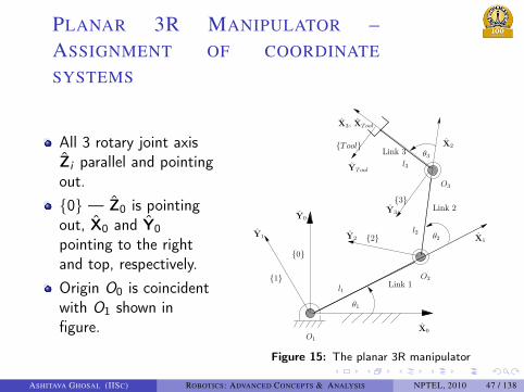
PLANAR 3R MANIPULATOR –ASSIGNMENT OF COORDINATE
SYSTEMS
All 3 rotary joint axisZi parallel and pointingout.{0} — Z0 is pointingout, X0 and Y0pointing to the rightand top, respectively.Origin O0 is coincidentwith O1 shown infigure.
{2}
{3}
YTool
X0
Y0
Link 1
{0}
{1}
Y1
O2
l1
O1
θ2
l2
l3
Link 3
O3
X2
Link 2
X3, XTool
{Tool}θ3
Y3
Y2 X1
θ1
Figure 15: The planar 3R manipulator
ASHITAVA GHOSAL (IISC) ROBOTICS: ADVANCED CONCEPTS & ANALYSIS NPTEL, 2010 47 / 138

. . . . . .
PLANAR 3R MANIPULATOR –ASSIGNMENT OF COORDINATE
SYSTEMS
For {1} origin O1 and Z1 are coincident with O0 and Z0.X1 and Y1 are coincident with X0 and Y0 when θ1 is zero.X1 is along the mutual perpendicular between Z1 and Z2.X2 is along the mutual perpendicular between Z2 and Z3.For {3}, X3 is aligned to X2 when θ3 = 0.O2 is located at the intersection of the mutualperpendicular along X2 and Z2.O3 is chosen such that d3 is zero.The origins and the axes of {1}, {2}, and {3} are shown inFigure 15.
ASHITAVA GHOSAL (IISC) ROBOTICS: ADVANCED CONCEPTS & ANALYSIS NPTEL, 2010 48 / 138

. . . . . .
PLANAR 3R MANIPULATOR – D-HTABLEFrom the assigned axes and origins, the D-H parameters are asfollows:
i αi−1 ai−1 di θi1 0 0 0 θ12 0 l1 0 θ23 0 l2 0 θ3
l1 and l2 are the link lengths and θi , i = 1,2,3 are rotaryjoint variables (see Figure 15).Length of the end-effector l3 does not appear in the table— Recall: D-H parameters are till the origin which is at thebeginning of a link!For end-effector frame, {Tool}:
Axis of {Tool} parallel to {3} → 3Tool [R] is identity matrix.
Origin of {Tool} at the mid-point of the parallel jawgripper, at a distance of l3 from O3 along X3.
ASHITAVA GHOSAL (IISC) ROBOTICS: ADVANCED CONCEPTS & ANALYSIS NPTEL, 2010 49 / 138

. . . . . .
PLANAR 3R MANIPULATOR – LINK
TRANSFORMS
Substitute elements of first row of D-H table in
equation (10) to get 01[T ] =
c1 −s1 0 0s1 c1 0 00 0 1 00 0 0 1
The second row of the D-H table gives
12[T ] =
c2 −s2 0 l1s2 c2 0 00 0 1 00 0 0 1
Finally, third row of D-H table gives
23[T ] =
c3 −s3 0 l2s3 c3 0 00 0 1 00 0 0 1
ASHITAVA GHOSAL (IISC) ROBOTICS: ADVANCED CONCEPTS & ANALYSIS NPTEL, 2010 50 / 138

. . . . . .
PLANAR 3R MANIPULATOR: LINK
TRANSFORMS (CONTD.)
The 3Tool [T ] is obtained as 3
Tool [T ] =
1 0 0 l30 1 0 00 0 1 00 0 0 1
To obtain 0
3[T ] multiply 01[T ] 1
2[T ] 23[T ] and get4
03[T ] =
c123 −s123 0 l1c1+ l2c12s123 c123 0 l1s1+ l2s120 0 1 00 0 0 1
To obtain 0
Tool [T ], multiply 03[T ] 3
Tool [T ]
0Tool [T ] =
c123 −s123 0 l1c1+ l2c12+ l3c123s123 c123 0 l1s1+ l2s12+ l3s1230 0 1 00 0 0 1
4The symbols s12, c123 denote sin(θ1+θ2) and cos(θ1+θ2+θ3),
respectively. Please see Notations in Module 0.ASHITAVA GHOSAL (IISC) ROBOTICS: ADVANCED CONCEPTS & ANALYSIS NPTEL, 2010 51 / 138

. . . . . .
PUMA 560 MANIPULATORThe PUMA 560 is a six-degree-of-freedom manipulator with allrotary joints — Figure 16 shows assigned coordinate systems.
X1
Y1
{1}
Z1
X2
Z2
Y2
{2}
O1, O2
X3
Y3
Z3
{3}O3
X4Y4
Z4
{4}
O4
a2
d3
(a) The PUMA 560 manipulator
d4
a3
Y3
X3 Z4
X4
Z6
X6
Y5
X5O3
{3}
{4}
{5}{6}
O4, O5, O6
(b) PUMA 560 - forearm and wrist
Figure 16: The PUMA 560 manipulator
ASHITAVA GHOSAL (IISC) ROBOTICS: ADVANCED CONCEPTS & ANALYSIS NPTEL, 2010 52 / 138

. . . . . .
PUMA 560 MANIPULATOR – D-HPARAMETERS
The D-H parameters for the PUMA 560 manipulator (seeFigure 16) are
i αi−1 ai−1 di θi
1 0 0 0 θ12 −π/2 0 0 θ23 0 a2 d3 θ34 −π/2 a3 d4 θ45 π/2 0 0 θ56 −π/2 0 0 θ6
Note: θi , i = 1,2, ...,6 are the six joint variables.
ASHITAVA GHOSAL (IISC) ROBOTICS: ADVANCED CONCEPTS & ANALYSIS NPTEL, 2010 53 / 138

. . . . . .
PUMA 560 MANIPULATOR – LINK
TRANSFORMS
Substituting elements of row #1 of D-H table and using
equation (10), we get 01[T ] =
c1 −s1 0 0s1 c1 0 00 0 1 00 0 0 1
From row # 2, we get 12[T ] =
c2 −s2 0 00 0 1 0
−s2 −c2 0 00 0 0 1
From row # 3, we get 23[T ] =
c3 −s3 0 a2s3 c3 0 00 0 1 d30 0 0 1
ASHITAVA GHOSAL (IISC) ROBOTICS: ADVANCED CONCEPTS & ANALYSIS NPTEL, 2010 54 / 138

. . . . . .
PUMA 560 MANIPULATOR: LINK
TRANSFORMS (CONTD.)
From row # 4 , we get 34[T ] =
c4 −s4 0 a30 0 1 d4
−s4 −c4 0 00 0 0 1
From row # 5 , we get 45[T ] =
c5 −s5 0 00 0 −1 0s5 c5 0 00 0 0 1
From row # 6 , we get 56[T ] =
c6 −s6 0 00 0 1 0
−s6 −c6 0 00 0 0 1
ASHITAVA GHOSAL (IISC) ROBOTICS: ADVANCED CONCEPTS & ANALYSIS NPTEL, 2010 55 / 138
. . . . . .
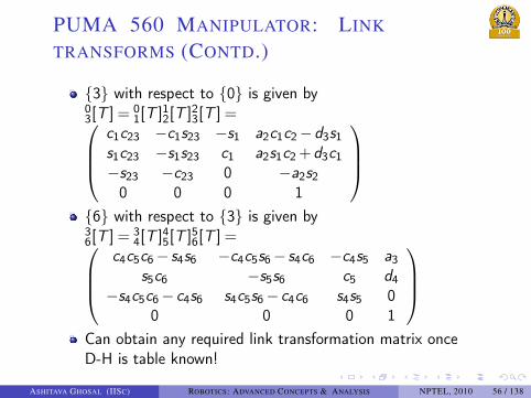
PUMA 560 MANIPULATOR: LINK
TRANSFORMS (CONTD.)
{3} with respect to {0} is given by03[T ] = 0
1[T ]12[T ]23[T ] =c1c23 −c1s23 −s1 a2c1c2−d3s1s1c23 −s1s23 c1 a2s1c2+d3c1−s23 −c23 0 −a2s2
0 0 0 1
{6} with respect to {3} is given by36[T ] = 3
4[T ]45[T ]56[T ] =c4c5c6− s4s6 −c4c5s6− s4c6 −c4s5 a3
s5c6 −s5s6 c5 d4−s4c5c6− c4s6 s4c5s6− c4c6 s4s5 0
0 0 0 1
Can obtain any required link transformation matrix onceD-H is table known!
ASHITAVA GHOSAL (IISC) ROBOTICS: ADVANCED CONCEPTS & ANALYSIS NPTEL, 2010 56 / 138
. . . . . .
SCARA MANIPULATOR
O0, O1 O2
θ1
θ2
d3
{ 1}
{ 2}
O3, O4
{ 3}
{ 4}
Z 1
X 1
Z 2
X 2
X
Z 3
θ4
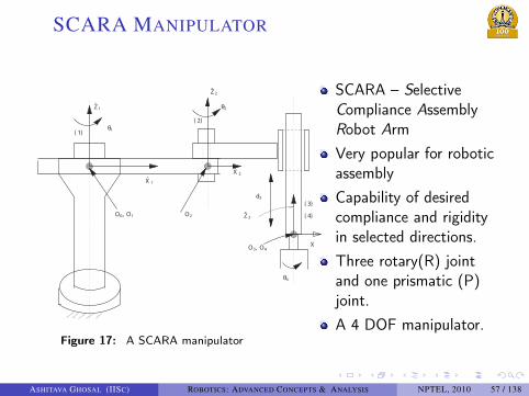
Figure 17: A SCARA manipulator
SCARA – SelectiveCompliance AssemblyRobot ArmVery popular for roboticassemblyCapability of desiredcompliance and rigidityin selected directions.Three rotary(R) jointand one prismatic (P)joint.A 4 DOF manipulator.
ASHITAVA GHOSAL (IISC) ROBOTICS: ADVANCED CONCEPTS & ANALYSIS NPTEL, 2010 57 / 138

. . . . . .
SCARA MANIPULATOR: D-HPARAMETERS
{0} and {1} have same origin & origins of {3} and {4}chosen at the base of the parallel jaw gripper.Directions of Z3 chosen pointing upward (see Figure 17).Note: Actual SCARA manipulator has ball-screw at thethird joint — We assume P joint.D-H Table for SCARA robot
i αi−1 ai−1 di θi1 0 0 0 θ12 0 a1 0 θ23 0 a2 −d3 04 0 0 0 θ4
ASHITAVA GHOSAL (IISC) ROBOTICS: ADVANCED CONCEPTS & ANALYSIS NPTEL, 2010 58 / 138

. . . . . .
SCARA MANIPULATOR – LINK
TRANSFORMS
Using equation (10) and the D-H table, link transforms can beobtained as
01[T ] =
c1 −s1 0 0s1 c1 0 00 0 1 00 0 0 1
, 12[T ] =
c2 −s2 0 a1s2 c2 0 00 0 1 00 0 0 1
23[T ] =
1 0 0 a20 1 0 00 0 1 −d30 0 0 1
, 34[T ] =
c4 −s4 0 0s4 c4 0 00 0 1 00 0 0 1
The transformation matrix 0
4[T ] is
04[T ] = 0
1[T ]12[T ]23[T ] 34[T ] =
c124 −s124 0 a1c1+a2c12s124 c124 0 a1s1+a2s120 0 1 −d30 0 0 1
ASHITAVA GHOSAL (IISC) ROBOTICS: ADVANCED CONCEPTS & ANALYSIS NPTEL, 2010 59 / 138

. . . . . .
PARALLEL MANIPULATORS
Extend idea of D-H parameters to a closed-loopmechanism/parallel manipulator.Key idea – Break a parallel manipulator into serialmanipulators.Obtain D-H parameters for serial manipulators.
Several ways to breakChoose one that leads to simple serial manipulators
During analysis – Combine serial manipulators usingconstraints
ASHITAVA GHOSAL (IISC) ROBOTICS: ADVANCED CONCEPTS & ANALYSIS NPTEL, 2010 60 / 138

. . . . . .
PARALLEL MANIPULATORS: 4-BAR
MECHANISM
l0
{L}
φ2
φ1
YL
XL
YR
XR
{R}
OL
OR
Link 1l1
l3
Link 2
Link 3
l2
θ1
Figure 18: A planar four-bar mechanism
Rotary joints 1 and4 fixed to ground attwo places.Break 4-barmechanism into twoserial manipulators.Break at joint 3 →A 2R planarmanipulator + a 1Rmanipulator
ASHITAVA GHOSAL (IISC) ROBOTICS: ADVANCED CONCEPTS & ANALYSIS NPTEL, 2010 61 / 138
. . . . . .
4-BAR MECHANISM – D-HPARAMETERS
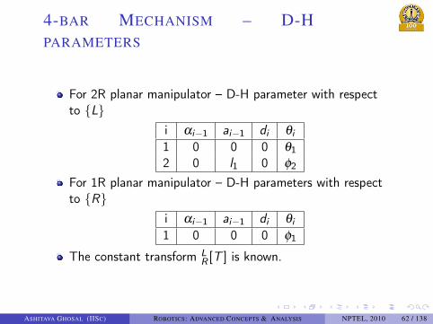
For 2R planar manipulator – D-H parameter with respectto {L}
i αi−1 ai−1 di θi1 0 0 0 θ12 0 l1 0 ϕ2
For 1R planar manipulator – D-H parameters with respectto {R}
i αi−1 ai−1 di θi1 0 0 0 ϕ1
The constant transform LR [T ] is known.
ASHITAVA GHOSAL (IISC) ROBOTICS: ADVANCED CONCEPTS & ANALYSIS NPTEL, 2010 62 / 138
. . . . . .
PARALLEL MANIPULATORS: THREE
DOF EXAMPLE
X
Y
ZMoving Platform
l3
l2
θ1
l1
θ2
θ3
p(x, y, z)
S1
S2S3
Axis of R1
Base Platform
Axis of R3
O
{Base}
Axis of R2
Figure 19: A three DOF parallelmanipulator
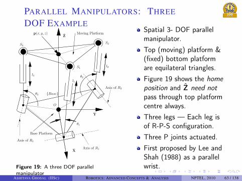
Spatial 3- DOF parallelmanipulator.Top (moving) platform &(fixed) bottom platformare equilateral triangles.Figure 19 shows the homeposition and Z need notpass through top platformcentre always.Three legs — Each leg isof R-P-S configuration.Three P joints actuated.First proposed by Lee andShah (1988) as a parallelwrist.
ASHITAVA GHOSAL (IISC) ROBOTICS: ADVANCED CONCEPTS & ANALYSIS NPTEL, 2010 63 / 138

. . . . . .
THREE DOF EXAMPLE: D-HPARAMETERS
D-H parameter for first leg with respect to {L1}i αi−1 ai−1 di θi1 0 0 0 ϕ12 −π/2 0 l1 0
D-H parameter for all R-P-S leg same except the referencecoordinate system.{L1}, {L2}, and {L3} are at the three rotary joints R1, R2,and R3, respectively.{Base} is located at the centre of the base platform &BaseLi
[T ], i = 1,2,3, are constant and known.Note: The angle θ1 shown in figure is same as π/2−ϕ1.
ASHITAVA GHOSAL (IISC) ROBOTICS: ADVANCED CONCEPTS & ANALYSIS NPTEL, 2010 64 / 138

. . . . . .
THREE DOF EXAMPLE: LINK
TRANSFORMATION MATRICES
L11 [T ] =
c1 −s1 0 0s1 c1 0 00 0 1 00 0 0 1
, 12[T ] =
1 0 0 00 0 1 l10 −1 0 00 0 0 1
2S1[T ] is an identity matrix – {S1} is located at the centre
of the spherical joint and parallel to {2}.BaseS1
[T ] = BaseL1
[T ]L11 [T ]12[T ]2S1
[T ]
Location of spherical joint S1 with respect to {Base} fromBaseS1
[T ] BaseS1 = (b− l1 cosθ1,0, l1 sinθ1)T , b is the
distance of R1 from the origin of {Base} (see figure 19).Location of S2 and S3BaseS2 = (−b
2 +12 l2 cosθ2,
√3b2 −
√3l22 cosθ2, l2 sinθ2)
T
BaseS3 = (−b2 +
12 l3 cosθ3,−
√3b2 +
√3l32 cosθ3, l3 sinθ3)
T
ASHITAVA GHOSAL (IISC) ROBOTICS: ADVANCED CONCEPTS & ANALYSIS NPTEL, 2010 65 / 138

. . . . . .
PARALLEL MANIPULATORS: SIX
DOF EXAMPLE
l13
l12l11
Z
l l l
l
ll
21 22 23
3132
33
θ
θ
θ
ψ
φ
ψ
φ
φψ
1
11
2
2
2
3
3b
b
b
1
2
3
pp
p
1
2
3
s
ss
dd
h
3
X
Y
Figure 20: A six DOF parallel (hybrid)manipulator
Moving platformconnected to fixed baseby three chains.Each chain is R-R-R &S joint at top.Model of athree-fingered hand(Salisbury, 1982)gripping an object withpoint contact andno-slip.Each finger modeledwith R-R-R joints andpoint of contactmodeled as S joint.
ASHITAVA GHOSAL (IISC) ROBOTICS: ADVANCED CONCEPTS & ANALYSIS NPTEL, 2010 66 / 138

. . . . . .
SIX DOF EXAMPLE: D-HPARAMETERS AND LINK TRANS-FORMS
D-H parameters for R-R-R chain.i αi−1 ai−1 di θi1 0 0 0 θ12 π/2 l11 0 ψ13 0 l12 0 ϕ1
D-H parameter does not contain last link length l13.D-H parameters for three fingers with respect to{Fi}, i = 1,2,3 identical.Can obtain transformation matrix Fi
pi [T ] by matrixmultiplication.
ASHITAVA GHOSAL (IISC) ROBOTICS: ADVANCED CONCEPTS & ANALYSIS NPTEL, 2010 67 / 138

. . . . . .
SIX DOF EXAMPLE: LINK
TRANSFORMS (CONTD.)
Position vector of spherical joint i
Fi pi =
cosθi (li1+ li2 cosψi + li3 cos(ψi +ϕi ))sinθi (li1+ li2 cosψi + li3 cos(ψi +ϕi ))
li2 sinψi + li3 sin(ψi +ϕi )
With respect to {Base}, the locations of {Fi}, i = 1,2,3,are known and constant (see Figure (20))Baseb1 = (0,−d ,h)T Baseb2 = (0,d ,h)T Baseb3 = (0,0,0)T
Orientation of {Fi}, i = 1,2,3, with respect to {Base} arealso known - {F1} and {F2} are parallel to {Base} and{F3} is rotated by γ about the Y (not shown in figure!).The transformation matrices Base
pi[T ] is
BaseF1
[T ]01[T ]12[T ]23[T ]3p1[T ] – Last transformation includes
l13.
ASHITAVA GHOSAL (IISC) ROBOTICS: ADVANCED CONCEPTS & ANALYSIS NPTEL, 2010 68 / 138

. . . . . .
SIX DOF EXAMPLE: LINK
TRANSFORMS (CONTD.)
Extract the position vector Basep1 from the last column ofBaseF1
[T ] Basep1 =Base b1+
F1 p1 = cosθ1(l11+ l12 cosψ1+ l13 cos(ψ1+ϕ1))−d + sinθ1(l11+ l12 cosψ1+ l13 cos(ψ1+ϕ1))
h+ l12 sinψ1+ l13 sin(ψ1+ϕ1)
Similarly for second leg
Basep2 =
cosθ2(l21+ l22 cosψ2+ l23 cos(ψ2+ϕ2))d + sinθ2(l21+ l22 cosψ2+ l23 cos(ψ2+ϕ2))
h+ l22 sinψ2+ l23 sin(ψ2+ϕ2)
For third leg Basep3 =
[R(Y,γ)]
cosθ3(l31+ l32 cosψ3+ l33 cos(ψ3+ϕ3))sinθ3(l31+ l32 cosψ3+ l33 cos(ψ3+ϕ3))
l32 sinψ3+ l33 sin(ψ3+ϕ3)
ASHITAVA GHOSAL (IISC) ROBOTICS: ADVANCED CONCEPTS & ANALYSIS NPTEL, 2010 69 / 138

. . . . . .
SUMMARY
D-H parameters obtained for serial manipulators – Planar3R, PUMA 560, SCARATo obtain D-H parameters for parallel manipulators
Break parallel manipulator into serial manipulators.Obtain D-H parameters for each serial chain.Examples of 4-bar mechanism, 3-degree-of-freedom and6-degree-of-freedom parallel manipulators.
Can extract position vectors of point of interest &orientation of links from link transforms.Kinematic analysis, using the concepts presented here,discussed in Module 3 and Module 4.
ASHITAVA GHOSAL (IISC) ROBOTICS: ADVANCED CONCEPTS & ANALYSIS NPTEL, 2010 70 / 138

. . . . . .
OUTLINE.. .1 CONTENTS.. .2 LECTURE 1
Mathematical PreliminariesHomogeneous Transformation
.. .3 LECTURE 2Elements of a robot – JointsElements of a robot – Links
.. .4 LECTURE 3Examples of D-H Parameters & Link TransformationMatrices
.. .5 LECTURE 4Elements of a robot – Actuators & Transmission
.. .6 LECTURE 5Elements of a robot – Sensors
.. .7 ADDITIONAL MATERIALProblems, References, and Suggested Reading
ASHITAVA GHOSAL (IISC) ROBOTICS: ADVANCED CONCEPTS & ANALYSIS NPTEL, 2010 71 / 138
. . . . . .
ACTUATORS FOR ROBOTS
Actuators are required to move joints, provide power anddo work.Serial robot actuators must be of low weight – Actuators ofdistal links need to be moved by actuators near the base.Parallel robots – Often actuators are at the base.Actuators drive a joint through a transmission deviceThree commonly used types of actuators:
HydraulicPneumaticElectric motors
ASHITAVA GHOSAL (IISC) ROBOTICS: ADVANCED CONCEPTS & ANALYSIS NPTEL, 2010 72 / 138

. . . . . .
ACTUATORS FOR ROBOTS
Source: http://www.hocdelam.org/vn/category/ho-tro/robotandcontrol/
Figure 21: Examples of actuators used in robots
ASHITAVA GHOSAL (IISC) ROBOTICS: ADVANCED CONCEPTS & ANALYSIS NPTEL, 2010 73 / 138

. . . . . .
ACTUATORS FOR ROBOTS –HYDRAULIC
Early industrial robots were driven by hydraulic actuators.Pump supplies high-pressure fluid (typically oil) to a linearcylinders, rotary vane actuator or a hydraulic motor at thejoint!Large force capabilities.Large power-weight ratio – The pump, electric motordriving the pump, accumulator etc. stationary and notconsidered in the weight calculation!Control is by means of on/off solenoid valves orservo-valves controlled electronically.The entire system consisting of Electric motor, pump,accumulator, cylinders etc. is bulky and often expensive –Limited to ‘big’ robots.
ASHITAVA GHOSAL (IISC) ROBOTICS: ADVANCED CONCEPTS & ANALYSIS NPTEL, 2010 74 / 138

. . . . . .
ACTUATORS FOR ROBOTS –PNEUMATIC
Similar to hydraulic actuators but working fluid is air.Similar to hydraulic actuators, air is supplied from acompressor to cylinders and flow of air is controlled bysolenoid or servo controlled valves.Less force and power capabilities.Less expensive than hydraulic drives.Chosen where electric drives are discouraged or for safetyor environmental reasons such as in pharmaceutical andfood packaging industries.Closed-loop servo-controlled manipulators have beendeveloped for many applications.
ASHITAVA GHOSAL (IISC) ROBOTICS: ADVANCED CONCEPTS & ANALYSIS NPTEL, 2010 75 / 138

. . . . . .
COMPARISON OF PNEUMATIC &HYDRAULIC ACTUATORS
Air used in pneumatic actuators is clean and safe.Oil in hydraulic actuator can be a health and fire hazardespecially if there is a leakage.Pneumatic actuators are typically light-weight, portableand faster.Air is compressible (oil is incompressible) and hencepneumatic actuators are ‘harder’ to control.Hydraulic actuators have the largest force/power densitycompared to any actuator.With compressors, accumulators and other components,the space requirement is larger than electric actuators.
ASHITAVA GHOSAL (IISC) ROBOTICS: ADVANCED CONCEPTS & ANALYSIS NPTEL, 2010 76 / 138

. . . . . .
ACTUATORS FOR ROBOTS –ELECTRIC MOTORS
Electric or electromagnetic actuators are widely used inrobots.Readily available in wide variety of shape, sizes, power andtorque range.Very easily mounted and/or connected with transmissionelements such as gears, belts and timing chains.Amenable to modern day digital control.Main types of electric actuators:
Stepper motorsPermanent magnet DC servo-motorBrushless motors
ASHITAVA GHOSAL (IISC) ROBOTICS: ADVANCED CONCEPTS & ANALYSIS NPTEL, 2010 77 / 138

. . . . . .
ELECTRIC ACTUATORS – STEPPER
MOTORS
Used in ‘small’ robots with small payload and “low” speeds.Stepper motors are of permanent magnet, hybrid orvariable reluctance type.Actuated by a sequence of pulses — For a single pulse,rotor rotates by a known step such that poles on stator androtor are aligned.Typical step size is 1.8◦ or 0.9◦.Speed and direction can be controlled by frequency ofpulses.Can be used in open-loop as cumulative error andmaximum error is one step!Micro-stepping possible with closed-loop feedback control.
ASHITAVA GHOSAL (IISC) ROBOTICS: ADVANCED CONCEPTS & ANALYSIS NPTEL, 2010 78 / 138

. . . . . .
STEPPER MOTORS
Parts of a Stepper Motor
http://www.engineersgarage.com/articles/stepper-motors
http://www.societyofrobots.com/member_tutorials/node/28 Variable Reluctance (VR) Stepper Motors
Number of teeth in the inner rotor (permanent magnet) is different than the number of teeth in stator. 1) Electro-magnet 1 is activated Rotor rotates up such that nearest teeth line up. 2) Electro-magnet 1 is deactivated and 2 is turned on Rotor rotates such that nearest teeth line up –
rotation is by a step (designed amount) of typically 1.8 or 0.9 degrees. 3) Electro-magnet 2 is deactivated and 3 is turned on Rotor rotates by another step. 4) Electro-magnet 3 is deactivated and 4 is turned on and cycle repeated.
Permanent Magnet (PM) Stepper Motors – Similar to VR but rotor is radially magnetized. Hybrid Stepper Motors – Combines best features of VR and PM stepper motors.
Figure 22: Stepper motor components and working principle
ASHITAVA GHOSAL (IISC) ROBOTICS: ADVANCED CONCEPTS & ANALYSIS NPTEL, 2010 79 / 138

. . . . . .
STEPPER MOTORS
Typically stepper motors have two phases.Four stepping modes
Wave drive – Only one phase/winding is on/energized →Torque output is smaller.Full step drive – Both phases are on at the same time →Rated performance.Half step drive – Combine wave and full-step drive →Angular movement half of first two.Micro-stepping – Current is varying continuously →Smaller than 1.8 or 0.9 degree step size, lower torque.
Choice of a stepper motor based on:Load, friction and inertia – Higher load can cause slipping!Torque-speed curve and quantities such as holding torque,pull-in and pull-out curve.Torque-speed characteristic determined by the drive –Bipolar chopper drives for best performance.Maximum slew-rate: maximum operating frequency withno load (related to maximum speed).
ASHITAVA GHOSAL (IISC) ROBOTICS: ADVANCED CONCEPTS & ANALYSIS NPTEL, 2010 80 / 138

. . . . . .
ELECTRIC ACTUATORS – DC/ACSERVO-MOTORS
Rotor is a permanent magnet and stator is a coil.Permanent magnets with rare earth materials(Samarium-Cobalt, Neodymium) can provide largemagnetic fields and hence high torques.Commutation done using brushes or in brushless motorusing Hall-effect sensors and electronics.Widely available in large range of shape, sizes, power andtorque range and low cost.Easy to control with optical encoder/tacho-generatorsmounted in-line with rotor.Brushless AC and DC servo-motors have low friction, lowmaintenance, low cost and are robust.
ASHITAVA GHOSAL (IISC) ROBOTICS: ADVANCED CONCEPTS & ANALYSIS NPTEL, 2010 81 / 138

. . . . . .
DC SERVO MOTORS
http://www.brushlessdcmotorparts.info http://www.rc-book.com/wiki Small RC Servo motors /brushless-electric-motor http://www.drivecontrol-details.info /rc-servo-motor.html
Slotted-brushless DC Servo motors Direct drive motor, Applimotion, Inc Brushless Hub motor for E-bike http://www.motioncontroltips.com/ http://news.thomasnet.com/ http://visforvoltage.org/ company_detail.html?cid=20082162 system-voltage/49-60-volts
Figure 23: Examples of DC servo motors
See also Wikipedia entry on electric motors.ASHITAVA GHOSAL (IISC) ROBOTICS: ADVANCED CONCEPTS & ANALYSIS NPTEL, 2010 82 / 138

. . . . . .
MODEL OF A DC PERMANENT
MAGNET MOTOR
ia
θm
LaR
a
Va
Motor
Figure 24: Model of a permanent magnet DCservo-motor
Rotor is apermanent magnet.Stator – Armaturecoil with resistanceRa and inductanceLa.Applied voltage Va,ia current in coil.Rotation speed ofmotor ˙θm –Mechanical part.
Torque developed Tm = Kt ia — Kt is constant.Back-emf V = Kg ˙θm — Kg is constant.Motor dynamics can be modeled as first-order ODE
La ia +Raia +Kg ˙θm = Va
Mechatronic model — Mechanical + Electrical/ElectronicsASHITAVA GHOSAL (IISC) ROBOTICS: ADVANCED CONCEPTS & ANALYSIS NPTEL, 2010 83 / 138
. . . . . .
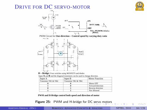
DRIVE FOR DC SERVO-MOTOR
PWM Circuit for One-direction – Control speed by varying duty ratio
H – Bridge: Four switches using MOSFETS and diodes Input A and B and the diagonal transistors can be used to change direction.
Input A Input B Motor Function Transistor TR1 & TR4 Transistor TR2 & TR4 0 0 Motor OFF 1 0 Forward direction 0 1 Reverse direction 1 1 Not Allowed
PWM and H-Bridge control both speed and direction of motor
Figure 25: PWM and H-bridge for DC servo motors
ASHITAVA GHOSAL (IISC) ROBOTICS: ADVANCED CONCEPTS & ANALYSIS NPTEL, 2010 84 / 138
. . . . . .
TRANSMISSIONS USED IN ROBOTS
Purpose of transmission is to transfer power from source toload.The purpose of a transmission is also to transfer power atappropriate speed.
Typical rated speed of a DC motor is between 1800 & 3600rpm.3000 rpm = 60 rps ≈ 360 radians/sec.For a (typical) 1 m link → Tip speed is 36 m/sec —Greater than speed of sound!Need for large reduction in speed.
Transmissions can (if needed) also convert rotary to linearmotion and vice-versa.Transmissions also transfer motion to different joints andto different directions.
ASHITAVA GHOSAL (IISC) ROBOTICS: ADVANCED CONCEPTS & ANALYSIS NPTEL, 2010 85 / 138

. . . . . .
TRANSMISSIONS USED IN ROBOTS
Transmissions in robots are decided based on motion, loadand power requirements, and by the placement of actuatorrelative to the joint.Transmissions for robots must be (a)stiff, (b) low weight,(c) backlash free, and (d) efficient.Direct drives with motor directly connected to joint. It hasadvantages of low friction and low backlash but areexpensive.Typical transmissions
Gear boxes of various kinds – Spur, worm and worm wheel,planetary etc..Belts and chain drives.Harmonic drive for large reduction.Ball screws and rack-pinion drives – To transform rotary tolinear motions.Kinematic linkages – 4-bar linkage.
ASHITAVA GHOSAL (IISC) ROBOTICS: ADVANCED CONCEPTS & ANALYSIS NPTEL, 2010 86 / 138

. . . . . .
TRANSMISSIONS USED IN ROBOTS
Figure 26: Examples of transmissions used in robots
ASHITAVA GHOSAL (IISC) ROBOTICS: ADVANCED CONCEPTS & ANALYSIS NPTEL, 2010 87 / 138

. . . . . .
OUTLINE.. .1 CONTENTS.. .2 LECTURE 1
Mathematical PreliminariesHomogeneous Transformation
.. .3 LECTURE 2Elements of a robot – JointsElements of a robot – Links
.. .4 LECTURE 3Examples of D-H Parameters & Link TransformationMatrices
.. .5 LECTURE 4Elements of a robot – Actuators & Transmission
.. .6 LECTURE 5Elements of a robot – Sensors
.. .7 ADDITIONAL MATERIALProblems, References, and Suggested Reading
ASHITAVA GHOSAL (IISC) ROBOTICS: ADVANCED CONCEPTS & ANALYSIS NPTEL, 2010 88 / 138

. . . . . .
INTRODUCTION
A robot without sensors is like a human being without eyes,ears, sense of touch, etc.
Sensor-less robots require costly/time consumingprogramming.Can perform only in “playback” mode.No change in their environment, tooling and work piececan be accounted for.
Sensors constitute the perceptual system of a robot,designed:
To make inferences about the physical environment,To navigate and localise itself,To respond more “flexibly” to the events occurring in itsenvironment, andTo enable learning, thereby endowing robots with“intelligence”.
Sensors allow less accurate modeling and control.Sensors enable robots to perform complex and increasedvariety of tasks reliably thereby reducing cost.
ASHITAVA GHOSAL (IISC) ROBOTICS: ADVANCED CONCEPTS & ANALYSIS NPTEL, 2010 89 / 138

. . . . . .
INTRODUCTION (CONTD.)
Dynamical systemChanges with time – Governed by differential equations.For a given input there is a well defined output.Linear dynamical system – Modeled by linear ordinarydifferential equations → Can be analysed using Laplacetransforms and transfer function5.
Control system is used toObtain desired response from dynamical system.Stabilize an unstable dynamical system.Improve performance.
Two kinds of system — Open-loop and closed-loop orfeedback control systems.Importance of sensors in modeling and control shown innext few slides.
5Other methods such as frequency domain analysis can also be used.ASHITAVA GHOSAL (IISC) ROBOTICS: ADVANCED CONCEPTS & ANALYSIS NPTEL, 2010 90 / 138
. . . . . .
OPEN-LOOP CONTROL SYSTEM
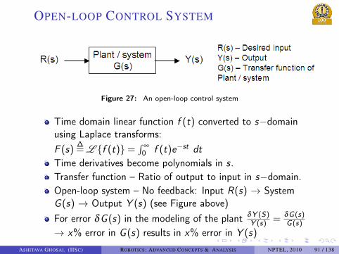
Figure 27: An open-loop control system
Time domain linear function f (t) converted to s−domainusing Laplace transforms:F (s) ∆
= L {f (t)}=∫ ∞0 f (t)e−st dt
Time derivatives become polynomials in s.Transfer function – Ratio of output to input in s−domain.Open-loop system – No feedback: Input R(s) → SystemG (s) → Output Y (s) (see Figure above)For error δG (s) in the modeling of the plant δY (S)
Y (s) = δG(s)G(s)
→ x% error in G (s) results in x% error in Y (s)
ASHITAVA GHOSAL (IISC) ROBOTICS: ADVANCED CONCEPTS & ANALYSIS NPTEL, 2010 91 / 138

. . . . . .
CLOSED-LOOP CONTROL SYSTEM
Figure 28: A closed-loop control system
Y (s) =D(s)G(s)
1+D(s)G(s)R(s); Chosen D(s)G(s)>> 1
For error δG (s) in the modeling of the plantδY (S)Y (s)
=δG(s)G(s)
11+D(s)G(s)
Since 1+D(s)G (s)>> 1 → x% error in G (s) results inmuch smaller error of
(1
1+D(s)G(s)
)x% in Y (s).
With sensors and feedback, less complex and expensivecontrollers and/or models of system can be used for morerobust performance.
ASHITAVA GHOSAL (IISC) ROBOTICS: ADVANCED CONCEPTS & ANALYSIS NPTEL, 2010 92 / 138

. . . . . .
CLOSED-LOOP CONTROL SYSTEM
Figure 29: Closed-loop control with sensors
Sensors must have low noise and be ‘good’ for effectiveness.Consider a ‘noisy’ sensor (see Figure above).Output of system
Y (s)=D(s)G (s)
1+D(s)G (s)(R(s)−N(s)); ChosenD(s)G (s)>> 1
Note that output is proportional to corrupted (R(s)−N(s))input, hence output error can never be reduced!
ASHITAVA GHOSAL (IISC) ROBOTICS: ADVANCED CONCEPTS & ANALYSIS NPTEL, 2010 93 / 138

. . . . . .
SENSORS IN ROBOTS
Sensor is a device to make a measurement of a physicalvariable of interest and convert it into electrical signal.Desirable features in sensors are
High accuracy.High precision.Linear response.Large operating range.Low response time.Easy to calibrate.Reliable and rugged.Low costEase of operation
Broad classification of sensors in robotsInternal state sensors.External state sensors.
ASHITAVA GHOSAL (IISC) ROBOTICS: ADVANCED CONCEPTS & ANALYSIS NPTEL, 2010 94 / 138

. . . . . .
SENSORS IN ROBOTS – INTERNAL
Internal sensors measure variables for controlJoint position.Joint velocity.Joint torque/force.
Joint position sensors (angular or linear)Incremental & absolute encoders — Optical, magnetic orcapacitive.Potentiometers.Linear analog resistive or digital encoders.
Joint velocity sensorsDC tacho-generator & resolver.sOptical encoders.
Force/torque sensors.At joint actuators for control.At wrist to measure components of force/moment beingapplied on environment.At end-effector to measure applied force on gripped object.
ASHITAVA GHOSAL (IISC) ROBOTICS: ADVANCED CONCEPTS & ANALYSIS NPTEL, 2010 95 / 138

. . . . . .
SENSORS IN ROBOTS – EXTERNAL
Detection of environment variables for robot guidance,object identification and material handling.Two main types – Contacting and non-contacting sensors.Contacting sensors: Respond to a physical contact
Touch: switches, Photo-diode/LED combination.Slip.Tactile: resistive/capacitive arrays.
Non-contacting sensors: Detect variations in optical,acoustic or electromagnetic radiations or change inposition/orientation.
Proximity: Inductive, Capacitive, Optical and Ultrasoni.cRange: Capacitive and Magnetic, Camera, Sonar, Laserrange finder, Structured light.Colour sensors.Speed/Motion: Doppler radar/sound, Camera,Accelerometer, Gyroscope.Identification: Camera, RFID, Laser ranging, Ultrasound.Localisation: Compass, Odometer, GPS.
ASHITAVA GHOSAL (IISC) ROBOTICS: ADVANCED CONCEPTS & ANALYSIS NPTEL, 2010 96 / 138
. . . . . .
SENSORS IN ROBOTS
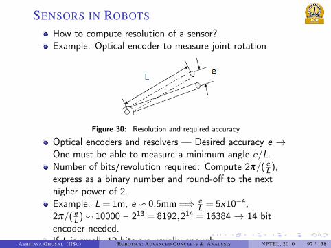
How to compute resolution of a sensor?Example: Optical encoder to measure joint rotation
Figure 30: Resolution and required accuracy
Optical encoders and resolvers — Desired accuracy e →One must be able to measure a minimum angle e/L.Number of bits/revolution required: Compute 2π/( e
L),express as a binary number and round-off to the nexthigher power of 2.Example: L = 1m, e v 0.5mm =⇒ e
L = 5x10−4,2π/( e
L)v 10000 – 213 = 8192,214 = 16384 → 14 bitencoder needed.If L is small, 12 bits are usually enough.ASHITAVA GHOSAL (IISC) ROBOTICS: ADVANCED CONCEPTS & ANALYSIS NPTEL, 2010 97 / 138
. . . . . .
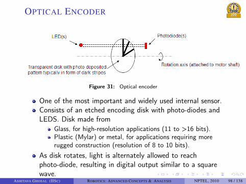
OPTICAL ENCODER
Figure 31: Optical encoder
One of the most important and widely used internal sensor.Consists of an etched encoding disk with photo-diodes andLEDS. Disk made from
Glass, for high-resolution applications (11 to >16 bits).Plastic (Mylar) or metal, for applications requiring morerugged construction (resolution of 8 to 10 bits).
As disk rotates, light is alternately allowed to reachphoto-diode, resulting in digital output similar to a squarewave.
ASHITAVA GHOSAL (IISC) ROBOTICS: ADVANCED CONCEPTS & ANALYSIS NPTEL, 2010 98 / 138

. . . . . .
OPTICAL ENCODER
Figure 32: Optical encoder outputs
Typically 3 signals available – Channel A, B and I; A and Bare phase shifted by 90 degrees and I is called as the indexpulse obtained every full rotation of disk.Signals read by a microprocessor/counter.Output of counter includes rotation and direction.Output can be absolute or relative joint rotation.Can be used for estimating velocity.
ASHITAVA GHOSAL (IISC) ROBOTICS: ADVANCED CONCEPTS & ANALYSIS NPTEL, 2010 99 / 138

. . . . . .
SENSORS FOR JOINT ROTATION
Potentiometers – Voltage ∝ resistance and resistance ∝rotation at joint
Not very accurate but very inexpensive.More suitable for slow rotations.Adds to joint friction.
Resolvers – Rotary electrical transformer to measure jointrotation
Analog output, need ADC for digital control.Electromagnetic device — Stator + Rotor (connected tomotor shaft).Voltage (at stator) ∝ sin(θ), θ = rotor angle.
Tachometers measures joint velocitySimilar to resolver.Voltage (at stator) ∝ θ , θ = angular velocity of the rotor.Analog output → ADC required for digital control.
ASHITAVA GHOSAL (IISC) ROBOTICS: ADVANCED CONCEPTS & ANALYSIS NPTEL, 2010 100 / 138
. . . . . .
FORCE/TORQUE SENSOR
Employed for force/torque sensing – Can be achieved byjoint and wrist sensing.Force/Torque joint sensors
Direct sensing of force/torque in a compliant shaftattached to motor by means of strain gages.A model of the motor and the shaft required.Introduced compliance at joint not desirable – Systemdynamics altered!For DC motor – Joint torque ∝ armature current.Requires model of motor & accuracy not very good.
Force/torque wrist sensorsMounted between end of robot arm and end-effector.Can measure all six components of force/torque usingstrain gages.Extensively used in force control.
ASHITAVA GHOSAL (IISC) ROBOTICS: ADVANCED CONCEPTS & ANALYSIS NPTEL, 2010 101 / 138
. . . . . .
FORCE/TORQUE SENSOR (CONTD.)
Performance specifications to ensure that the wrist motionsgenerated by the force/torque sensors do not affect theposition accuracy of the manipulator:
High stiffness to ensure quick dampening of the disturbingforces which permits accurate readings during short timeintervals.Compact design to ensure easy movement of themanipulator.Need to be placed close to end-effector/tool.Linear relation between applied force/torque and straingauge readings.Made from single block of metal → No hysteresis.
ASHITAVA GHOSAL (IISC) ROBOTICS: ADVANCED CONCEPTS & ANALYSIS NPTEL, 2010 102 / 138

. . . . . .
FORCE/TORQUE WRIST SENSOR
Figure 33: Six axisforce/torque sensors at wrist
F = [RF ]W
wherea
RF =0 0 r13 0 0 0 r17 0
r12 0 0 0 r25 0 0 00 r32 0 r34 0 r36 0 r380 0 0 r44 0 0 0 r480 r52 0 0 0 r56 0 0
r61 0 r63 0 r65 0 r67 0
F = (Fx ,Fy ,Fz ,Mx ,My ,Mz)
T .W = (w1,w2,w3,w4,w5,w6,w7,w8).wi are the 8 strain gauge readings.
aThe formula can be derived from statics,please see Module 0, Lecture 5.
Rij are found during calibration process using least-squaretechniques.
ASHITAVA GHOSAL (IISC) ROBOTICS: ADVANCED CONCEPTS & ANALYSIS NPTEL, 2010 103 / 138

. . . . . .
EXTERNAL SENSORS – TOUCH
Allows a robot or manipulator to interact with itsenvironment – to “touch and feel”, “see” and “locate”.Two classes of external sensors – Contact and non-contact
Figure 34: Touch sensor
Simple – LED-Photo-diodepair used to detectpresence/absence of objectto be graspedMicro-switch to detecttouch.
ASHITAVA GHOSAL (IISC) ROBOTICS: ADVANCED CONCEPTS & ANALYSIS NPTEL, 2010 104 / 138

. . . . . .
EXTERNAL SENSORS – SLIP
Figure 35: Slip sensor
Slip sensor to detect if grasped object is slipping.Free moving dimpled ball – Deflects a thin rod on the axisof a conductive diskEvenly spaced electrical contacts placed under diskObject slips past the ball, moving rod and disk – Electricalsignal from contact to detect slip.Direction of slip determined from sequence of contacts.
ASHITAVA GHOSAL (IISC) ROBOTICS: ADVANCED CONCEPTS & ANALYSIS NPTEL, 2010 105 / 138

. . . . . .
EXTERNAL SENSORS – TACTILE
Figure 36: Robot hand with tactilearray
“Skin” like membrane to“feel” the shape of thegrasped objectAlso used to measureforce/torque required tograsp objectChange inresistance/capacitance dueto local deformation fromapplied force
ASHITAVA GHOSAL (IISC) ROBOTICS: ADVANCED CONCEPTS & ANALYSIS NPTEL, 2010 106 / 138

. . . . . .
EXTERNAL SENSORS – TACTILE
(CONTD.)
Figure 37: Artificial Skin
Send current in one set,measure current in othersetMagnitude of current ∝change in resistance due todeformationMagnitude of current ∝change in capacitance
Fluid filled membraneArray of Hall-effect sensorsMEMS – Silicon micro-machined with doped strain-gaugeflexure
ASHITAVA GHOSAL (IISC) ROBOTICS: ADVANCED CONCEPTS & ANALYSIS NPTEL, 2010 107 / 138

. . . . . .
EXTERNAL SENSORS – PROXIMITY
Detect presence of an object near a robot or manipulatorWorks at very short ranges (<15-20 mm)Frequently used in stationary and mobile robots to avoidobstacles and for safety during operationFour main types of proximity sensors
Inductive proximity sensorsCapacitive proximity sensorUltrasonic proximity sensorOptical proximity sensors
ASHITAVA GHOSAL (IISC) ROBOTICS: ADVANCED CONCEPTS & ANALYSIS NPTEL, 2010 108 / 138

. . . . . .
INDUCTIVE PROXIMITY SENSOR
Figure 38: A magnetic proximity sensor
Electronic proximity sensor based on change of inductance.Detects metallic objects without touching them.Consists of a wound coil, located next to a permanentmagnet, packaged in a simple housing.
ASHITAVA GHOSAL (IISC) ROBOTICS: ADVANCED CONCEPTS & ANALYSIS NPTEL, 2010 109 / 138

. . . . . .
INDUCTIVE PROXIMITY SENSOR –MAGNETIC
Figure 39: Flux lines in a magnetic sensor
Ferromagnetic material enters or leaves the magnetic field→ Flux lines of the permanent magnet change theirposition.Change in flux → Induces a current pulse with amplitudeand shape proportional to rate of change in flux.
ASHITAVA GHOSAL (IISC) ROBOTICS: ADVANCED CONCEPTS & ANALYSIS NPTEL, 2010 110 / 138
. . . . . .
INDUCTIVE PROXIMITY SENSOR –MAGNETIC
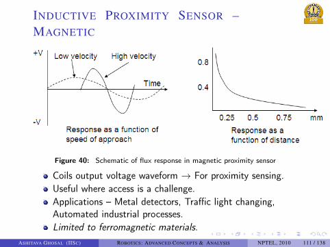
Figure 40: Schematic of flux response in magnetic proximity sensor
Coils output voltage waveform → For proximity sensing.Useful where access is a challenge.Applications – Metal detectors, Traffic light changing,Automated industrial processes.Limited to ferromagnetic materials.
ASHITAVA GHOSAL (IISC) ROBOTICS: ADVANCED CONCEPTS & ANALYSIS NPTEL, 2010 111 / 138

. . . . . .
INDUCTIVE – HALL EFFECT
PROXIMITY SENSOR
Hall effect relates the voltage between two points in aconducting or semiconducting material subjected to astrong magnetic field across the material.When a semi-conductor magnet device is brought in closeproximity of a ferromagnetic material
the magnetic field at the sensor weakens due to bending ofthe field lines through the material,the Lorentz forces are reduced, andthe voltage across the semiconductor is reduced.
The drop in the voltage is used to sense the proximity.Applications: Ignition timings in IC engines, tachometersand anti-lock braking systems, and brushless DC electricmotors.
ASHITAVA GHOSAL (IISC) ROBOTICS: ADVANCED CONCEPTS & ANALYSIS NPTEL, 2010 112 / 138

. . . . . .
CAPACITIVE PROXIMITY SENSORS
Figure 41: Capacitive sensor
Change in
Capacitance
Figure 42: Capacitive sensor response
Similar to inductive, but uses electrostatic field.Can sense metallic as well as non-metallic materials.Sensing element is a capacitor composed of a sensitiveelectrode and a reference electrode.
ASHITAVA GHOSAL (IISC) ROBOTICS: ADVANCED CONCEPTS & ANALYSIS NPTEL, 2010 113 / 138
. . . . . .
CAPACITIVE PROXIMITY SENSORS
Object’s entry in electrostatic field of electrodes changescapacitance.Oscillations start once capacitance exceeds a predefinedthreshold.Triggers output circuit to change between on and off.When object moves away, oscillator’s amplitude decreases,changing output back to original state.Larger size and dielectric constant of target, means largercapacitance and easier detection.Useful in level detection through a barrier.
ASHITAVA GHOSAL (IISC) ROBOTICS: ADVANCED CONCEPTS & ANALYSIS NPTEL, 2010 114 / 138

. . . . . .
ULTRASONIC PROXIMITY SENSORS
Electro-acoustic transducer to send and receive highfrequency sound waves.Emitted sonic waves are reflected by an object back to thetransducer which switches to receiver mode.Same transducer is used for both receiving and emittingthe signals – Fast damping of acoustic energy is essentialto detect close proximity objects.Achieved by using acoustic absorbers and by decoupling thetransducer from its housing.Typically of low resolution.Important specifications – 1) Maximum operating distance,2) Repeatability, 3) Sonic cone angle, 4) Impulse frequency,and 5) Transmitter frequency.Some well-known applications – 1) Useful in difficultenvironments, 2) Liquid level detection and 3) Car parkingsensors.
ASHITAVA GHOSAL (IISC) ROBOTICS: ADVANCED CONCEPTS & ANALYSIS NPTEL, 2010 115 / 138

. . . . . .
OPTICAL PROXIMITY SENSORS
Also known as light beam sensors – Solid state LED actingas a transmitter by generating a light beam.A solid-state photo-diode acts as a receiver.Field of operation of the sensor – Long pencil like volume,formed due to intersection of cones of light from sourceand detector.Any reflective surface that intersects the volume getsilluminated by the source and is seen by the receiver.Generally a binary signal is generated when the receivedlight intensity exceeds a threshold value.Applications: 1) Fluid level control, 2) Breakage and jamdetection, 3) Stack height control, box counting etc.
ASHITAVA GHOSAL (IISC) ROBOTICS: ADVANCED CONCEPTS & ANALYSIS NPTEL, 2010 116 / 138
. . . . . .
RANGE SENSORS
Measure distance of objects at larger distances.Uses electromagnetic or electrostatic or acoustic radiation –Looks for changes in the field or return signal.Highly reliable with long functional life and no mechanicalparts.Four main kinds of range sensing techniques in robots
Triangulation.Structured lighting approach.Time of flight range finders.Vision .
Applications: 1) Navigation in mobile robots, 2) Obstacleavoidance, 3) Locating parts, etc.
ASHITAVA GHOSAL (IISC) ROBOTICS: ADVANCED CONCEPTS & ANALYSIS NPTEL, 2010 117 / 138

. . . . . .
RANGE SENSORS – TRIANGULATION
Figure 43: Triangulation
A narrow beam of lightsweeps the plane definedby the detector, the objectand the source,illuminating the target.Detector output is peakwhen illuminated patch isin front.With B and θ known →Obtain D = B tanθ .Changing B and θ , onecan get D for all visibleportions of object.
Very little computation required.Very slow as one point is done at a time.
ASHITAVA GHOSAL (IISC) ROBOTICS: ADVANCED CONCEPTS & ANALYSIS NPTEL, 2010 118 / 138

. . . . . .
RANGE SENSORS – STRUCTURED
LIGHTING
Figure 44: Structured lighting
A ’“sheet” of lightgenerated through acylindrical lens or narrowslit is projected on a target.Intersection of the sheetwith target yields a lightstripe.A camera offset slightlyfrom the projector, viewsand analyze the shape ofthe line.
ASHITAVA GHOSAL (IISC) ROBOTICS: ADVANCED CONCEPTS & ANALYSIS NPTEL, 2010 119 / 138

. . . . . .
RANGE SENSORS – STRUCTURED
LIGHTING
Distortion of the line is related to distance and can becalculated.Horizontal displacement (in image) proportional to depthgradient.Integration gives absolute range.Calibration is required.Advantages:
Fast, very little computation is required.Can scan multiple points or entire view at once.
Structured lighting should be permitted.
ASHITAVA GHOSAL (IISC) ROBOTICS: ADVANCED CONCEPTS & ANALYSIS NPTEL, 2010 120 / 138

. . . . . .
RANGE SENSORS – TIME-OF-FLIGHT
Utilizes pulsed lasers and ultrasonics to measure time takenby the pulse to coaxially return from a surface.If D is the target’s distance, c is the speed of radiation,and t is elapsed time taken for the pulse to return
D =ct2
Light or electromagnetic radiation more useful for large(kilometers) distances.Light not very suitable in robotic applications as c is large.
To measure range with ±0.25 inch accuracy, one needs tomeasure very small time intervals – v 50 ps.
Suitable for acoustic (ultrasonic) radiation, since c v 330m/s.Can only detect distance of one point in its view — Scanrequired for object.
ASHITAVA GHOSAL (IISC) ROBOTICS: ADVANCED CONCEPTS & ANALYSIS NPTEL, 2010 121 / 138

. . . . . .
RANGE SENSORS – TIME-OF-FLIGHT
Phase shift and continuous laser light for measuring distance
Figure 45: Range measurement using phaseshift
Laser beam ofwavelength λ split –Two beams travel todetector through twodifferent paths.Phase delay betweentwo beams is measured.Distance traveled byfirst beam L.Total distance traveledby the second beamD ′ = L+2D →D ′ = L+ θ
360λ , θ is thephase shift.
ASHITAVA GHOSAL (IISC) ROBOTICS: ADVANCED CONCEPTS & ANALYSIS NPTEL, 2010 122 / 138
. . . . . .
RANGE SENSORS – TIME-OF-FLIGHT
For θ = 360◦, two waveforms are aligned and D ′ = L andD ′ = L+nλ → Waveforms cannot be differentiated onphase shift alone.Restrict θ < 360◦ and 2D < λ
D =θ
360(λ2)
λ typically small → Impractical for robot application →Modulate laser light with a waveform of much higherwavelength.Example: modulating frequency=10 MHz → λ = c
f = 30mand D up to 15m can be measured.Advantages of continuous light technique
Yields intensity as well range information,Requires very little computation,Lasers do not suffer from specular reflection, andExpensive, not so robust and require higher power.
ASHITAVA GHOSAL (IISC) ROBOTICS: ADVANCED CONCEPTS & ANALYSIS NPTEL, 2010 123 / 138

. . . . . .
RANGE SENSORS – ULTRASONIC
Similar to the pulsed laser technique.An ultrasonic chirp is transmitted over a short time period.From the time difference between the transmitted andreflected wave, D can be obtained.Generally used for navigation and obstacle avoidance inrobots.Much cheaper than laser range finder.Shorter range as waves disperse.Wavelength of ultrasonic radiation much larger → Notreflected very well from small objects and corners.Ultrasonic waves not reflected very well from plastics andsome other materials.
ASHITAVA GHOSAL (IISC) ROBOTICS: ADVANCED CONCEPTS & ANALYSIS NPTEL, 2010 124 / 138

. . . . . .
VISION SENSORS
Most powerful and complex form of sensing, analogous tohuman eyes.Comprising of one or more video cameras with integratedsignal processing and imaging electronics.Includes interfaces for programming and data output, and avariety of measurement and inspection functions.Also referred to as machine or computer vision.Computations required are very large compared to anyother form of sensing.Computer vision can be sub-divided into six main areas: 1)Sensing, 2) Pre-processing, 3) Segmentation, 4)Description, 5) Recognition and 6) Interpretation.
ASHITAVA GHOSAL (IISC) ROBOTICS: ADVANCED CONCEPTS & ANALYSIS NPTEL, 2010 125 / 138

. . . . . .
VISION SENSORS
Three levels of processing.Low level vision
Primitive in nature, requires no intelligence on the part ofthe vision functions.Sensing and pre-processing can be considered as low levelvision functions.
Medium level vision
Processes that extract, characterize and label componentsin an image resulting from a low level vision.Segmentation, description and recognition of the individualobjects refer to the medium level function.
High level vision: Processes that attempt to emulatecognition.
ASHITAVA GHOSAL (IISC) ROBOTICS: ADVANCED CONCEPTS & ANALYSIS NPTEL, 2010 126 / 138

. . . . . .
VISION SENSORS
Smaller number of robotic applications – Primarily due tocomputational complexity and low speed.Vision system can
Determine distances of objects.Determine geometrical shape and size of objects.Determine optical (color, brightness) properties of objectsin an environment.Can be used for navigation (map making), obstacleavoidance, Cartesian position and velocity feedback,locating parts, and many other uses.Can learn about environment.Acquire knowledge and intelligence.
Vision systems extensively used in autonomous navigationin mobile robots (Mars rovers).Use of vision systems increasing rapidly as technologyimproves!
ASHITAVA GHOSAL (IISC) ROBOTICS: ADVANCED CONCEPTS & ANALYSIS NPTEL, 2010 127 / 138

. . . . . .
NEW DEVELOPEMENTS IN SENSOR
TECHNOLOGY – MEMS SENSORS
Consist of very small electrical, electronics and mechanicalcomponents integrated on a single chip.Provide an interface to sense, process and/or control thesurrounding environment.Generally silicon based, allowing integration withmicroelectronics.Sensing mechanisms employed are a) Capacitive, b)Piezoelectric, c) Piezoresistive, d) Ferroelectric, e)Electromagnetic and f) Optical.Capacitive sensing most successful due to a) Norequirement of exotic materials, b) Low power consumptionand c) Stability over temperature ranges.
ASHITAVA GHOSAL (IISC) ROBOTICS: ADVANCED CONCEPTS & ANALYSIS NPTEL, 2010 128 / 138

. . . . . .
MEMS SENSORS (CONTD.)
Figure 46: A typical MEMS capacitivesensor
Polysilicon springs suspendMEMS structure above thesubstrate – Proof mass isfree to move in X and Ydirection.Radial fingers fixed toproof mass are positionedbetween plates fixed to thesubstrate.Each finger and pair offixed plates make up adifferential capacitor.
In-plane acceleration causes the proof mass to moverelative to the plates changing the capacitance.Change in capacitance converted to a voltage signal.Can sense dynamic and static acceleration.
ASHITAVA GHOSAL (IISC) ROBOTICS: ADVANCED CONCEPTS & ANALYSIS NPTEL, 2010 129 / 138
. . . . . .
MEMS SENSORS (CONTD.)
Applications of MEMS Sensors:Automotive electronics and crash systems.High resolution seismic sensing.Medical equipments.Hard disk drives.Computer peripherals.Wireless devices.Smart portable devices such as phones, PDAs etc.
MEMS sensors are finding their way into mobile robots.
ASHITAVA GHOSAL (IISC) ROBOTICS: ADVANCED CONCEPTS & ANALYSIS NPTEL, 2010 130 / 138

. . . . . .
MOEMS SENSORS
MOEMS stands for Micro-opto-electromechanical systems.Silica based MEMS sensors, though very effective, cannotbe used in high temperature and pressure conditions, dueto the limiting mechanical and electrical properties of silica.For harsh environmental conditions, MEMS sensors arebuilt out of robust materials such as (Si, SiC) and areintegrated with optical signal detection technique formingMOEMS.MOEMS sensors are highly resistant to electromagneticinterference (EMI) and radio frequency interference (RFI).Eliminate the need for on-board electronics.
ASHITAVA GHOSAL (IISC) ROBOTICS: ADVANCED CONCEPTS & ANALYSIS NPTEL, 2010 131 / 138

. . . . . .
SMART SENSORS
Figure 47: Components of a smart sensor
“Smart Sensor” – A single device combining data collectionand information output.As per IEEE 1451.2, a smart sensor is:“a transducer that provides functions beyond thosenecessary for generating a correct representation of asensed or control quantity”.Integration of transducer + applications + networking.Evolving concept – Often sensors not complying with IEEEdefinition are also called smart sensors!
ASHITAVA GHOSAL (IISC) ROBOTICS: ADVANCED CONCEPTS & ANALYSIS NPTEL, 2010 132 / 138

. . . . . .
SMART SENSORS (CONTD.)
Three primary kinds of smart sensors:Transmitter plus micro-controller capable of a certainamount of internal signal processing, such as linearisation,conversion to engineering units, diagnostics etc.A sensor that can communicate over a digitalcommunications network, either wired or wireless.A smart plug-and-play transducer electronic data sheet(TEDS) sensor with applications in aerospace and defense,transportation and research labs.
Smart sensors are capable of a) self identification anddiagnosis, b) Time and location awareness for time andposition stamping, c) Conform to standard datacommunications and control protocols for interoperability.Other features of smart sensors – a)remote diagnostics, b)improved reliability, and c) better signal to noise ratio.
ASHITAVA GHOSAL (IISC) ROBOTICS: ADVANCED CONCEPTS & ANALYSIS NPTEL, 2010 133 / 138
. . . . . .
INTELLIGENT SENSORS
For advanced robotic devices, large amount of sensoryinformation slows down the controller.Intelligent sensors take some load off the controller by
Taking some predefined action based on the input received.Efficiently and precisely measuring the parameters,enhancing or interrupting them.
Intelligent sensors: An adaptation of smart sensors withembedded algorithms for detection of noise,instrumentation anomalies and sensor anomalies.Enabling technology for ISHM (Integrated Systems HealthManagement) used in spaceships by NASA.
ASHITAVA GHOSAL (IISC) ROBOTICS: ADVANCED CONCEPTS & ANALYSIS NPTEL, 2010 134 / 138

. . . . . .
SENSOR-BASED ROBOTICS – ASMIOASIMO: Advanced Step in InnovativeMObility.A humanoid robot developed byHONDA car company of Japan.
Sensors for vision, speed, balance,force, angle, and foot area.34 degrees of freedom controlled byservo motors.
Capable of advanced movementWalking and running.Maintaining posture and balance.Climbing stairs & avoiding obstacle.
IntelligenceCharting a shortest route.Recognizing moving objects.Distinguish sounds and recognizefaces and gestures.
Figure 48: ASIMOclimbing stairs
Figure 49: ASIMOplaying soccer
ASHITAVA GHOSAL (IISC) ROBOTICS: ADVANCED CONCEPTS & ANALYSIS NPTEL, 2010 135 / 138

. . . . . .
SENSORS IN ROBOTS – SUMMARY
Sensors enhance performance of robots/manipulators, andmake them more flexible. for different application.Two main types of sensors
Internal sensors for measuring variables such as jointrotation, velocity, force, and torque.External sensors for measuring variables such as proximity,touch, range, and geometry.
Large varieties of sensors exist for large variety ofmeasurement tasks.More than one sensor is typically used in a robot.Vision system is the most powerful and complex sensor.New and modern sensor technologies are becoming matureand are finding their way into robots.
ASHITAVA GHOSAL (IISC) ROBOTICS: ADVANCED CONCEPTS & ANALYSIS NPTEL, 2010 136 / 138

. . . . . .
OUTLINE.. .1 CONTENTS.. .2 LECTURE 1
Mathematical PreliminariesHomogeneous Transformation
.. .3 LECTURE 2Elements of a robot – JointsElements of a robot – Links
.. .4 LECTURE 3Examples of D-H Parameters & Link TransformationMatrices
.. .5 LECTURE 4Elements of a robot – Actuators & Transmission
.. .6 LECTURE 5Elements of a robot – Sensors
.. .7 ADDITIONAL MATERIALProblems, References, and Suggested Reading
ASHITAVA GHOSAL (IISC) ROBOTICS: ADVANCED CONCEPTS & ANALYSIS NPTEL, 2010 137 / 138

. . . . . .
ADDITIONAL MATERIAL
Exercise ProblemsReferences & Suggested ReadingHomogeneous coordinates, lines & screws
Please see Known Bugs in Module 0, slide #10 forviewing links.To view above links
Copy link and paste in a New Window/Tab by right click.Close new Window/Tab after viewing.
ASHITAVA GHOSAL (IISC) ROBOTICS: ADVANCED CONCEPTS & ANALYSIS NPTEL, 2010 138 / 138


![Finale 2005 - [CAVALGADA] · PDF fileroberto carlos arr. manoel ferreira & & & & & & & & & & & & & &?????](https://img.pdfslide.us/doc/110x75/5a72754e7f8b9a9d538d9075/finale-2005-cavalgadawww2secultcegovbrrecursospublicwebbancopdf.jpg)