Robot Navigation With PolyMap, a Polygon-based Map Format

Robot Navigation With PolyMap, a Polygon-based MapFormat

Johann Dichtl, Xuan S. Le, Guillaume Lozenguez, Luc Fabresse, and Noury Bouraqadi

IMT Lille Douai, Univ. Lille, Unité de Recherche Informatique et Automatique, F-59000 Lille,France

[email protected]

Abstract. Vector-based map formats such as PolyMap are more compact in termof memory footprint compared with regular occupancy grid map formats. Thesparse nature of a PolyMap along with the explicit representation of traversablespace and frontiers makes it suitable for mono and multi-robot autonomous ex-ploration.In this paper, we propose a PolyMap-based navigation stack suitable for au-tonomous exploration. This navigation stack internally relies on a topologicalgraph that is automatically computed from a PolyMap. This graph is critical tosignificantly reduce the search space when computing a global path comparedwith traditional occupancy grid maps. We also discuss two optimizations to speedup path planning computation on this graph. Our experiments demonstrate the ef-ficiency of our PolyMap-based navigation stack.

Keywords: Mobile Robot Navigation; Vector-Based Map; Topological-based Nav-igation

1 Introduction

Mobile robots heavily rely on accurate representations of their environment (namedmaps) to fulfill their tasks. Maps are often restricted to 2D as a direct result of thecapabilities of the sensors mounted on the robot. Building a map is a Chicken-and-Egg-Problem because it requires the current location of the robot while localization requiresa map. Simultaneous Localization and Mapping (SLAM) tackle this problem using fewmajor techniques such as: Bayes-based Filters [20] (Kalman Filters [9], Particle Filters[6]) and Graph-Based SLAM [8,11]. Most SLAM algorithms use an occupancy gridrepresentation for the map (grid-based maps) in which each cell of the grid depicts asmall area as either obstacle, free space, or unknown space.

The size of grid-based maps is directly related to the size of the mapped environmentand the resolution of the map i.e. how much space is represented by one cell. This mem-ory consuming representation is a critical issue especially in the context of a multi-robotautonomous exploration scenario [17]. Indeed, while robots are exploring the environ-ment, they continuously update their map of the environment. The updated map mustthen be shared over wireless with other robots or even human operators/supervisors ifany. In these scenarios, the occupancy grid map format is inefficient because it requiresa lot of bandwidth and it limits the frequency of map exchanges [1].

2 Johann Dichtl et al.

There are other map formats such as feature-based or vector-based maps. The workpresented in this paper relies on PolyMap [3] because it is a compact vector-basedformat and it is suitable for autonomous exploration thanks to an explicit representationof frontiers [4,10]. In a nutshell (cf. Section 3 for further details), a PolyMap is made ofsimple polygons represented by line segments. A line segment can represent differentthings such as a frontier that delimits the transition between explored and unexploredspace.

In multi-robots autonomous exploration scenarios, frontiers are used to prioritizeareas of interest and reduce the global exploration time by optimizing the assignmentof frontiers to different robots. This optimization problem requires to compute a lotof paths from target frontiers to robots’ positions. Indeed, each robot must select (orbe assigned) a frontier to explore among several candidates accordingly to the pathto reach them (e.g. select the closest frontier). This optimization problem is dynamicbecause the global map changes as well as frontiers. In this context, computing paths iskey and must be efficient.

This papers focuses on global navigation on a PolyMap i.e. computing a path fromthe robot’s current position to a target area. This task cannot be directly performed ona PolyMap. Transforming a PolyMap into a grid-based map is not an option in termsof memory and processing consumptions. In this paper, we propose a navigation stackthat computes a topological graph from a PolyMap. From the theoretical point of view,this topological graph reduces the search space when computing paths. We also reporton experimentations that shows the efficiency of this solution when it is implementedwith specific data structures.

This paper is organized as follows. Section 2 presents a state of the art of navigationsolutions for mobile robots. Section 3 presents the PolyMap format used to representthe robot environment. In Section 4, we describe our main contribution that consistsin a PolyMap-based navigation stack. This involves a building process of a topologi-cal graph out of a PolyMap and its challenges. Section 5 reports on experiments thatvalidate the approach in simulation on different terrains. We also present two differ-ent optimizations that make our navigation stack more efficient as shown in the latestresults. Section 6 concludes this papers and draws some perspectives of this work formulti-robots systems.

2 State of the Art of Robot Navigation

Autonomous navigation for exploration requires the robot to perceive and to estimatethe obstacle shapes to plan a safe path to a target position. This state of the art presentsfour families of approaches that tackle this problem. Given our objective presented inintroduction, we are particularly interested in the required computing resources and thedependencies to a specific map model of each family.

2.1 Reactive navigation

Reactive navigation consists in computing the robot movement instantaneously accord-ingly to its current perception. Bug algorithm [16] for instance, guarantees the robot

PolyMap Based Robot Navigation 3

to attain a reachable target, in static environment, by moving along obstacles on therobot’s trajectory. Reactive navigation requires: the local perception of obstacles, anefficient continuous localization of the robot, and the position of the goal. No specificlocalization technique or map format are required. However, the lack of global planningtypically leads to suboptimal robot trajectories.

2.2 Grid-based Navigation

Several approaches are based on a regular decomposition of the environment into cellssuch as Occupancy Grid Maps to compute an efficient trajectory from the robot posi-tion to a target position. For instance, an approach based on potential field [2] guidesthe robot with repulsive forces spread from the obstacles and an attractive force directedtoward the target. Like other regular-cells-navigation approaches (as based on MarkovDecision Process [5]), the action performed in a cell depends on an evaluation of neigh-boring cells. The trajectory planning requires several iterations on the complete map toconverge to a stable configuration, driving a robot towards one and only one target. Theresulting trajectory could be classified as optimal regarding the cell dimension. How-ever, it requires computation that rapidly become unpractical in large environment or inmulti-task and multi-robot scenario.

2.3 Heuristic approaches

To speed up computation, heuristic approaches compute paths on a graph (adjacenttraversable cells) that is built from Occupancy Grid Maps produced by most SLAMalgorithms. A textbook case is provided with the Robot Operating System (ROS) mod-ule move_base1[15]. Some well-known path planning algorithms, such as Dijistra, A∗,Navfn, etc. are employed on a graph generated from a Grid Map where obstacle shapesare inflated. This way, the approach returns the shortest path to a target position whilethe robot keep safe distances to obstacles.

These approaches based on converting Grid Maps usually lead to generate largeand hard to process graphs making path planning slow. Approaches based on Rapidlyexploring Random Tree [12] tackle this problem by performing the A∗ algorithm whileiteratively building a tree (instead of a graph) at the same time. At each iteration, randommovements toward the target position generate new reachable positions from the mostpromising ones. In case of a dead end (all random movements fail because of obstaclesin the map), a backtrack mechanism is activated. The algorithm ends when the target isreached or when no more position in the tree can be extended. Each path computationrequires to build a new tree.

2.4 Topology-based Navigation

Generally, topology-based navigation (as proposed in [14]) relies on an hybrid reac-tive/deliberative architecture. Reactive modules control the robot movement toward“easily reachable” positions and are supervised by deliberative modules. Deliberative

1 https://wiki.ros.org/move_base - Author: Eitan Marder-Eppstein

https://wiki.ros.org/move_base


modules are responsible for SLAM and path planning where a path is defined as a suc-cession of reachable positions accordingly to the reactive capabilities. Ideally, a robotshould use a graph with a minimum number of nodes and edges to fastly compute thosepath between any couple of positions. Nodes represent significant area (room corner, in-tersection, etc.) and edges model the capability of a robot to move from a node positionto another.

Topological navigation could be directly based on topological mapping [13] with aloss on the obstacles shaping. More classically, a topological map would be generatedfrom a grid map as a Voronoi [19] (graph built with the farthest paths to the obstacles) ora Visibility Graph (obstacle corner positions connected while a free straight line exists).From our knowledge, there is no Visibility Graph approach proposed to handle on-linecomputations in exploration context.

2.5 Summary

In this paper, we investigate topology-based navigation with a topological graph gen-erated from a PolyMap. The PolyMap structure is close to a topological graph and re-quires fewer computations, which will permit to efficiently supervise robot movementsto a target.

3 Overview of the PolyMap Format

This PolyMap [3] format provides advantages over occupancy grids in terms of mem-ory footprint, and does not fall behind in visualization compared to pure topologicalmaps. This is a significant advantage when the map needs to be updated frequentlyover a wireless connection. Additionally the explicit modeling of frontiers helps withautonomous exploration. The sparse nature of the map format also provides advantageswhen it comes to navigation tasks, as we will show in this paper. But, first we need tofurther present more formally the PolyMap format before building our new navigationstack on top of it.

3.1 Model

PolyMap represents the environment using simple polygons. Simple polygons are non-self-intersecting closed polygons [7]. Our polygons model only explored space, i.e. theinside of all polygons is traversable space. Formally, a PolyMap M is defined as:

type : T = {obstacle, frontier, sector} (1)

vector : V = {(a, b, t)|a, b ∈ R2; a 6= b; t ∈ T} (2)polygon : P = {vi|i ≥ 3; vi ∈ V } (3)

PolyMap : M = {pi|1 ≤ i ≤ n; pi ∈ P} (4)

with pi being a simple polygon, and n being the number of polygons forming the map.We define three types of line segments :


Obstacles: they represent the outline of obstacles.Frontiers: they model the transition from free/traversable space to unknown/unexplored

space.Sectors: they delimit a traversable transition between the polygon the vector belongs

to and another adjacent polygon.

Each line segment has exactly one type, polygons can contain line segments of dif-ferent types. The direction of line segments is chosen, so that clockwise oriented poly-gons contain traversable space inside. Figure 1 shows an example of map containingtwo different types of line segments: red line segments represent obstacles and yellowline segments represent sectors.

Fig. 1: A PolyMap example. The left figure shows the map itself, the right figure hasthe polygons moved apart to show the four individual polygons that make up this map.

3.2 BSP-Tree Representation

As with other map formats (e.g. grid map), a PolyMap can be obtained via a SLAMprocess. We have developed PolySLAM, an algorithm that builds a PolyMap map di-rectly from raw sensor data (e.g. laser data). We will not detail this algorithm here sinceit is beyond the scope of this writing and deserves a dedicated paper. However, to in-troduce the BSP-Tree representation of PolyMaps, we need to introduce the concept ofKeyframes used by PolySLAM.

Starting from raw sensor scans, PolySLAM produces Keyframes. Those are simplepolygons, that represent the space surrounding a robot at a given point within the map’sreferential. Each new keyframe represents new acquired knowledge of the environment.It is then merged into the existing map during the SLAM.

To improve the speed of the merging keyframes into a PolyMap, we represent themap using a Binary Space Partitioning Tree (BSP-Tree) [18]. A BSP-Tree is a tree datastructure. Each node of a BSP-Tree holds a hyperplane that partitions the hyperspace intwo parts, while the leaves hold objects localized in the areas of hyperspace, separated


by hyperplanes. PolyMap is a format for 2D maps. Hence, objects are polygons, whilehyperplanes are 2D splitting lines. The left sub-tree for a splitting line gathers polygonslocated on one side of the line. Polygons in the right sub-tree are located at the otherside. Figure 2 shows a PolyMap where splitting lines of the BSP-tree visible.

-5

-4

-3

-2

-1

0

1

2

3

4

-6 -4 -2 0 2 4

4

3

4

3

2

1

21

0

map t=1

Fig. 2: Example of a PolyMap represented in a BSP-tree. Splitting lines are displayedas black dashed lines.

To merge a new keyframe into a PolyMap, the polygon that represents the keyframeis inserted into the BSP-tree. We start at the splitting line that is the root of the BSP-tree, and go down until reaching a leave. For each splitting line, we go either left orright depending the side of the splitting line where the polygon is located.

If a polygon intersects with a splitting line then it is cut into smaller polygons. Thedecomposition is done in a way to ensure that each of these new polygons lies on onlyone side of the 2D line. Last, these new polygons are inserted into the BSP-tree.

4 PolyMap-based Navigation

A PolyMap is a compact map format suitable to accurately represent a space. But, ituses a BSP-Tree data structure that is not directly suitable for navigation. Therefore, weneed to build a topological graph out of the BSP-Tree.

4.1 Numerical Problems to Consider

To build a topological graph, we need to determine which polygons share overlappingvectors of type sector. While this looks like an easy task at first glance, there are a fewdetails that make this more tricky then expected. The first problem is, that we cannotjust look for an identical vector with start and end points reversed, since vectors mayoverlap without sharing any common start or end points. This is illustrated in Figure 3in which the opposing horizontal vectors either share the start or end point, but never


both. Note, that in this example the vertical sector borders do share both start and endpoints.

1

2

3

4

5

6

1 2 3 4 5 6 7

1

2

3

4

5

6

1 2 3 4 5 6 7

Fig. 3: An example of sector borders partial overlapping with vectors on the other sideof the splitting line. The left figure shows the map embedded into a BSP tree with threesplitting lines. The right figure highlights the overlapping vectors in question.

The second problem is, that computing whether two given lines (extending two vec-tor that we want to test) are collinear is numerically challenging. For example, the natureof how computers store float point numbers makes it highly likely, that two lines/vectorsthat should be considered collinear have a slightly different orientation. And for sim-ilar reasons, it is possible that for example the start or end point of a vector does notexactly lie on a line that is collinear to the vector. Adding a tolerance to similarity testson the other hand provides us with the problem, that we may encounter false positiveswhen testing for overlapping vectors. We circumvent this problem by using the BSP-tree structure that created the sector-typed vectors in the first place, as explained in thenext section.

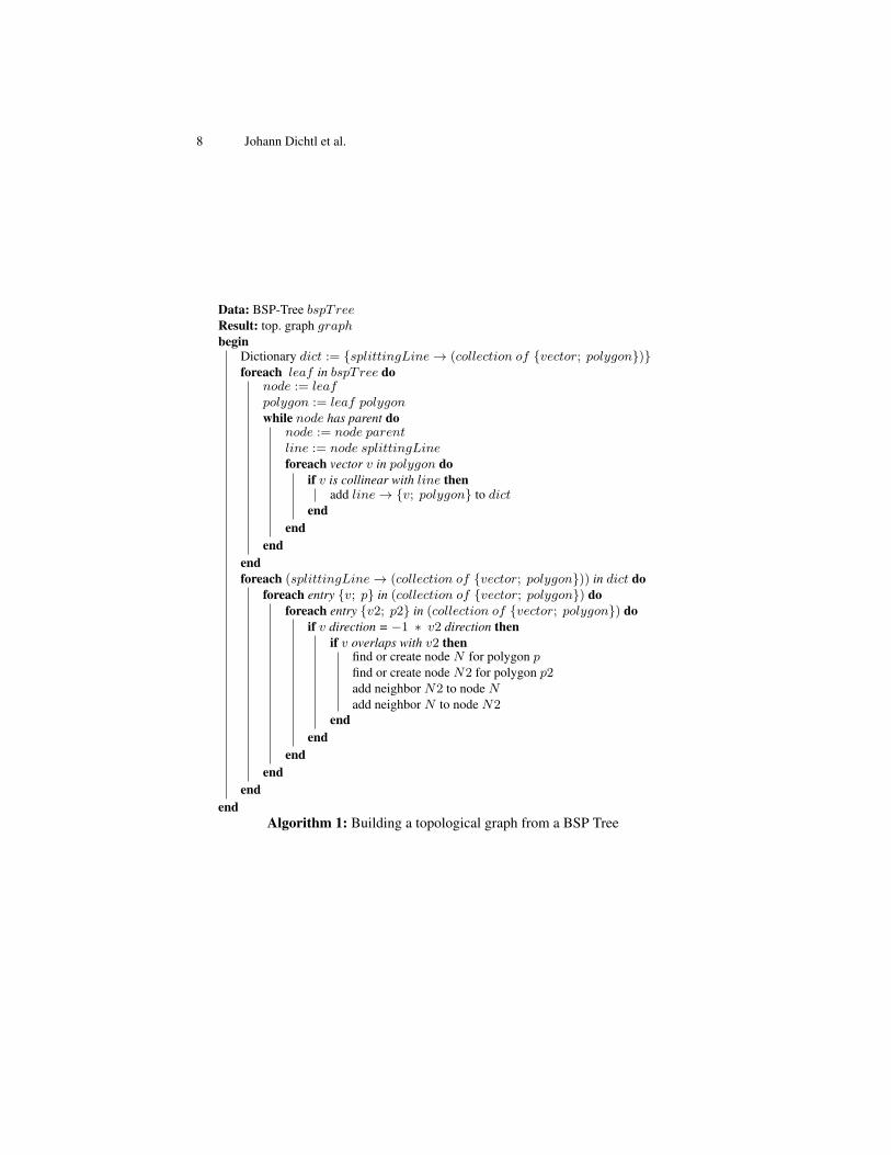
4.2 From BSP-Tree to Topological Graph

By construction, every sector-typed vector is adjacent to a a splitting line in the BSP-Tree. Therefor, instead to consider all vectors of the map, we can narrow down poten-tially overlapping vectors to those that lie on the same splitting line. The structure ofthe BSP-Tree makes this convenient and relatively fast, assuming that the tree itself isbalanced. Once we have collected all vectors that lie on the same splitting line, we com-pute which ones overlap. Now we can add edges to the graph for each polygon that issharing an overlapping vector with a polygon on the other side of the splitting line. Thisis done by adding the corresponding neighbors to the node that represents the polygonin the graph (and creating new nodes if the respective polygons are not already repre-sented in the graph). This process creates a topological graph based on the PolyMap,which is considerably more sparse than a graph based on a conventional grid map.


Data: BSP-Tree bspTreeResult: top. graph graphbegin

Dictionary dict := {splittingLine→ (collection of {vector; polygon})}foreach leaf in bspTree do

node := leafpolygon := leaf polygonwhile node has parent do

node := node parentline := node splittingLineforeach vector v in polygon do

if v is collinear with line thenadd line→ {v; polygon} to dict

endend

endendforeach (splittingLine→ (collection of {vector; polygon})) in dict do

foreach entry {v; p} in (collection of {vector; polygon}) doforeach entry {v2; p2} in (collection of {vector; polygon}) do

if v direction = −1 ∗ v2 direction thenif v overlaps with v2 then

find or create node N for polygon pfind or create node N2 for polygon p2add neighbor N2 to node Nadd neighbor N to node N2

endend

endend

endend

Algorithm 1: Building a topological graph from a BSP Tree


4.3 Path Planning on a Topological Graph

Once a topological graph has been build it can be used to compute the path to a targetlocation in the environment. The first step is to determine the current location of therobot in the topological graph. For this we select the polygon that contains the centerof the robot. This can be done efficiently since we have the map stored in a BSP-Treewhich allows us to just walk down the tree on whichever side of the splitting lines therobot’s center is located. The polygon can then be used to identify the correspondingnode in the topological graph. This will act as our starting node for a conventional A?

or D?light graph search. For the final result of our graph search, we replace the firstnode with a temporary node that contains the robot’s current location instead, since weotherwise would use the polygon’s center for further computations.

A simple example is illustrated in Figure 4, which shows navigation on a small map.The robot is located at the bottom part of the map, labeled ’start’. The target area is inthe top right corner of the map, labeled ’goal’. With the map placed in a BSP-Tree, it ispartitioned into smaller polygons, indicated by the yellow lines. Each leaf in the BSP-Tree is linked to a node in the graph via the polygon that both share. In this examplethe topological graph (colored pink) contains eleven nodes. With an A? graph searchwe are able to find a valid path from the robot’s position to the target area, as shown inthe right figure.

-0.5

0

0.5

1

1.5

2

2.5

3

3.5

-0.5 0 0.5 1 1.5 2 2.5 3 3.5

-0.5

0

0.5

1

1.5

2

2.5

3

3.5

-0.5 0 0.5 1 1.5 2 2.5 3 3.5

start

goal

Fig. 4: Navigation example on a small map. The left figure shows the map portionedinto smaller areas, with the topological graph overlayed. The right figure shows thecomputed path that leads from the start location to the target area.

5 Experiments and Optimizations

5.1 First results

First tests show that the concept of building a topological graph from a PolyMap is fea-sible. But at the same time, we find that the topological graph created this way has not


yet reached its full potential. When building a PolyMap with keyframes that containnoise, we no longer have perfect alignment of vectors, and as a result, the PolyMapcontains a considerable amount of small polygons that are clustered around obstacles.Furthermore, the incremental map building from keyframes promotes long thin poly-gons along the newly explored areas. There are nodes of the topological graph that areessentially inaccessible by any robot because they are too close to obstacles is obviouslyundesirable. And long thin polygons are also less desirable than more compact shapedpolygons, since the latter are more “local” representation of the environment, and leadsin general to less zigzag-shaped trajectories. Both issues can be solved easily, as shownin the following.

5.2 Using Grid Partitioning on the PolyMap

Our solution to prevent a build-up of excessively long thin polygons is to impose a gridstructure on the map. All polygons that span over a grid line are split on the respectiveline, and the new polygons are treated separately. This breaks up all large polygonsinto smaller polygons and provides a more even distribution of nodes in the topologicalgraph as a result. Compared to conventional grid maps, our cell dimension is relativelylarge: 1 by 1 meter by default. Each occupied cell contains a BSP-Tree, like the originalPolyMap format, but now limited in its dimension to the size of the grid cell. This setupallows us to quickly access polygons, first by determining which grid cell we need,and then by searching within the BSP tree of the cell. Lookup of the cell typically isdone in O(1) time complexity (basically a 2D table lookup), and finding elements inthe BSP tree (if balanced) takes log(N) time, with N being the number of elements inthe tree. This also removes any worries about unbalanced BSP-Trees, since the individ-ual trees are now much smaller, so that even a degenerated tree wont pose a problemperformance-wise.

We formally define the GridPolyMap as follows:

cell : C = {r|r ∈M} (5)GridPolyMaph : G = {mi,j |1N;mi,j ∈ C} (6)

The GridPolyMap G is a two dimensional grid where each entry contains a cell C.A cell in return contains a map M as defined in (4), stored in a BSP-Tree.

An direct comparison between a map with and without grid overlay can be seenin Figure 5. By separating parts of the maps into individual cells we prevent the largerpolygons to be split into smaller ones when the merging process introduces new splittinglines, because the splitting lines in one cell do not affect any other cells.

5.3 Removing Inaccessible Nodes from the Graph

When the size of the robot is known, we can take the robot footprint into account toremove nodes from the graph that are not accessible by the robot. As a quick heuristicwe remove all nodes from the graph where the polygons center point is closer to an ob-stacle than the radius of the robot. Since we typically experience a lot of small polygonsaround obstacles, this reduces the size of the graph by a significant amount. In fact, the


Fig. 5: Comparison of a PolyMap versus a GridPolyMap. The environment is a longwide corridor that exceeds the robots maximum sensor range. The incremental updatesfrom the moving robot add long thin slices to the explored area, which are visible in thetwo figures. However the right figure has a grid overlay, which splits long polygons intosmaller ones.


number of nodes and edges is reduced by about two orders of magnitude in our tests.An example can be seen in Figure 6, where the number of nodes in the graph dropsfrom 62427 to 688. The robot radius used in this example was 0.25m.

Fig. 6: The left figure shows the full topological graph of the map, drawn on top ofthe actual map. The right figure shows the pruned graph with all inaccessible nodesremoved.

5.4 Experiment Results

To test the impact of our optimizations, we created a topological graph for a few ofmaps. The map has been created with our PolySLAM algorithm, using data collectedfrom a simulated environment. Table 1 shows the results with and without pruning thetopological graph. We can see a significant reduction of the graph size in all cases. Wealso notice, that the grid overlay increases the number of nodes by only a moderateamount.

Map Format full graph prunedPolyMap 60786 676

Gri

dPol

yMap

(gri

dsi

zein

met

er)

0.5 78972 18371.0 63279 8852.0 62427 6884.0 62289 670

Table 1: Size of the topological graph (node count) for various map configurations.


We also created a topological graph from an occupancy grid representing an officeenvironment (16m by 16m in size) and compared the performance. The occupancy gridhas been inflated by 0.25m to make the results comparable to our pruned graph of theGridPolyMap, which also removed nodes that are closer than 0.25m to any obstacle.When creating the graph for the occupancy grid, we consider the 8 closest neighborsfor each cell, allowing for horizontal, vertical, and diagonal edges. Table 2 and Figure 7are showing the results of our experiment. With 72475 nodes, the graph computed fromthe occupancy grid is relatively large with respect of the environment. In comparison,the graph for the GridPolyMap only contains 688 nodes – two orders of magnitude less.Similarly, the A∗ search requires significantly less iterations to reach the target on ourGridPolyMap-derived topological graph. However, while the path for the occupancygrid contains more nodes, the actual distance is shorter. The reason for this is that thepath for the GridPolyMap is not as close to the obstacles, and contains more zigzag-likemovements.

Fig. 7: Navigation on an Occupancy Grid in comparison to a GridPolyMap. The left im-age shows the resulting path on the occupancy grid, the right image on a GridPolyMap.The pink background in the left image visualizes the traversable area after inflating allobstacles. The pink lines in the right image represent the edges of the topological graph.

Graph source node count path node count path lengthOccupancy Grid 72475 344 19.45m

GridPolyMap 688 39 25.06mTable 2: Comparison of the topological graph created from an occupancy grid and cre-ated from a GridPolyMap. The computed path in visualized in Figure 7.


6 Conclusion

In this paper, we introduce a solution for autonomous robot navigation based on PolyMap,a lightweight polygon-based map format. PolyMap represents a terrain using a BSP-Tree where leaves are polygons of traversable space. We have shown how to build atopological graph out of this BSP-Tree. Thanks to the vectorial nature of PolyMap, theresulting topological graph is considerably sparse. Compared to traditional grid-basedmaps, our solution allows faster path planning, while still using a conventional A∗ orD∗light algorithms.

Although these results are already interesting per se, we have demonstrated thatwe can go beyond thanks to two optimizations. First, based on a grid-based partition-ing of the map, we have drastically reduced the complexity of the searching for poly-gons within PolyMap. The second optimization consists into taking into account therobot footprint while building the topological graph. This allows to dismiss unreachablenodes, resulting into a smaller topological graph. Experiments validate the effectivenessof these optimizations.

As with future work, we plan to use our solution to perform multi-robot exploration.We expect to benefit from the lightweight nature of PolyMap, and the resulting topo-logical graph to reduce the network bandwidth required by robot data exchange. This iscritical in a context where robots need to setup an ad hoc communication network.

Acknowledgment

This work was completed in the framework of DataScience project which is co-financedby European Union with the financial support of European Regional Development Fund(ERDF), French State and French Region of Hauts-de-France.


References

1. Baizid, K., Lozenguez, G., Fabresse, L., Bouraqadi, N.: Vector Maps: A Lightweight andAccurate Map Format for Multi-robot Systems. In: International Conference on IntelligentRobotics and Applications, Springer International Publishing (2016) 418–429

2. Barraquand, J., Langlois, B., Latombe, J.C.: Numerical potential field techniques for robotpath planning. IEEE Transactions on Systems, Man and Cybernetics 22 (1992) 224–241

3. Dichtl, J., Fabresse, L., Lozenguez, G., Bouraqadi, N.: Polymap: A 2d polygon-based mapformat for multi-robot autonomous indoor localization and mapping. In: International Con-ference on Intelligent Robotics and Applications, Springer (2018) 120–131

4. Faigl, J., Kulich, M.: On benchmarking of frontier-based multi-robot exploration strategies.In: 2015 European Conference on Mobile Robots (ECMR). (Sept 2015) 1–8

5. Foka, A.F., Trahanias, P.E.: Real-time hierarchical POMDPs for autonomous robot naviga-tion. Robotics and Autonomous Systems 55(7) (2007) 561–571

6. Grisetti, G., Stachniss, C., Burgard, W.: Improved techniques for grid mapping with rao-blackwellized particle filters. IEEE Transactions on Robotics 23(1) (Feb 2007) 34–46

7. Grünbaum, B.: Convex Polytopes. Volume 221. Springer Science & Business Media (2013)8. Hess, W., Kohler, D., Rapp, H., Andor, D.: Real-time loop closure in 2D LIDAR SLAM. Pro-

ceedings - IEEE International Conference on Robotics and Automation 2016-June (2016)1271–1278

9. Huang, S., Dissanayake, G.: Convergence and consistency analysis for extended kalmanfilter based slam. IEEE Transactions on Robotics 23(5) (Oct 2007) 1036–1049

10. Juliá, M., Gil, A., Reinoso, O.: A comparison of path planning strategies for autonomousexploration and mapping of unknown environments. Autonomous Robots 33(4) (2012) 427–444

11. Konolige, K., Grisetti, G., Kümmerle, R., Burgard, W., Limketkai, B., Vincent, R.: Efficientsparse pose adjustment for 2d mapping. In: 2010 IEEE/RSJ International Conference onIntelligent Robots and Systems. (Oct 2010) 22–29

12. Kuffner, J., LaValle, S.: RRT-connect: An efficient approach to single-query path planning.In: International Conference on Robotics and Automation. Volume 2. (2000) 995–1001

13. Kuipers, B.: The Spatial Semantic Hierarchy. Artificial Intelligence 119 (2000) 191–23314. Lozenguez, G., Adouane, L., Beynier, A., Martinet, P., Mouaddib, A.I.: Interleaving Planning

and Control of Mobiles Robots in Urban Environments Using Road-Map. In: InternationalConference on Intelligent Autonomous Systems. (2012)

15. Marder-Eppstein, E., Berger, E., Foote, T., Gerkey, B., Konolige, K.: The office marathon:Robust navigation in an indoor office environment. In: Robotics and Automation (ICRA),2010 IEEE International Conference on, IEEE (2010) 300–307

16. McGuire, K., de Croon, G., Tuyls, K.: A comparative study of bug algorithms for robotnavigation. CoRR abs/1808.05050 (2018)

17. Saeedi, S., Trentini, M., Li, H., Seto, M.: Multiple-robot Simultaneous Localization andMapping - A Review 1 Introduction 2 Simultaneous Localization and Mapping : problemstatement. Journal of Field Robotics (2015)

18. Thibault, W.C., Naylor, B.F.: Set operations on polyhedra using binary space partitioningtrees. SIGGRAPH Comput. Graph. 21(4) (August 1987) 153–162

19. Thrun, S.: Learning Metric-Topological Maps for Indoor Mobile Robot Navigation. Artifi-cial Intelligence 99(1) (1998) 21–71

20. Thrun, S., Burgard, W., Fox, D.: Probabilistic Robotics (Intelligent Robotics and Au-tonomous Agents). The MIT Press (2005)

Documents

Robot Navigation With PolyMap, a Polygon-based Map Format