Embed Size (px)
Citation preview
Robotics and Autonomous Systems 30 (2000) 39–64
A mobile robot employing insect strategies for navigation
Dimitrios Lambrinosa, Ralf Möllera,b,∗, Thomas Labhartb, Rolf Pfeifera, Rüdiger Wehnerba AI Lab, Department of Computer Science, University of Zurich, Winterthurerstrasse 190, 8057 Zurich, Switzerland
b Department of Zoology, University of Zurich, Winterthurerstrasse 190, 8057 Zurich, Switzerland
Abstract
The ability to navigate in a complex environment is crucial for both animals and robots. Many animals use a combinationof different strategies to return to significant locations in their environment. For example, the desert antCataglyphisis ableto explore its desert habitat for hundreds of meters while foraging and return back to its nest precisely and on a straight line.The three main strategies thatCataglyphisis using to accomplish this task arepath integration, visual pilotingandsystematicsearch. In this study, we use a synthetic methodology to gain additional insights into the navigation behavior ofCataglyphis.Inspired by the insect’s navigation system we have developed mechanisms for path integration and visual piloting that weresuccessfully employed on the mobile robotSahabot 2. On the one hand, the results obtained from these experiments providesupport for the underlying biological models. On the other hand, by taking the parsimonious navigation strategies of insectsas a guideline, computationally cheap navigation methods for mobile robots are derived from the insights gained in theexperiments. ©2000 Elsevier Science B.V. All rights reserved.
Keywords:Insect navigation; Robot navigation; Polarization vision; Path integration; Visual landmark navigation
1. Introduction
In recent years the idea of “learning from nature” israpidly spreading through a number of scientific com-munities: computer science (artificial intelligence, ar-tificial evolution, artificial life), engineering (bionics),and robotics (biorobotics). The main goal is to exploitthe impressive results achieved by the blind but potentdesigner “Evolution”. Among the most awesome ca-pabilities exhibited by natural systems are the naviga-tional skills of insects. Despite their diminutive brains,many insects accomplish impressive navigation tasks.Desert antsCataglyphis, for example, make foragingexcursions that take them up to 200 m away from their
∗ Corresponding author. Tel: +41-1-63-65722; fax: +41-1-63-56809.E-mail address:[email protected] (R. Möller).
nest. On finding a suitable prey, they return home un-failingly and in a straight line [47] (see Fig. 1).
Cataglyphiscannot use pheromones to retrace itstrail in order to return back to its nest, since thepheromones evaporate in a few seconds because ofthe high ground temperatures. More than two decadesof field work (for a review see [50]) have revealedmany details about the behavioral repertoire and theunderlying mechanisms thatCataglyphis employswhen homing. The three main strategies used arepathintegration, visual piloting, and systematic search[52]. Whereas path integration based on compassinformation gained from the polarization pattern ofthe sky is the primary navigation strategy of the ants,geocentered information based on landmarks is alsoused in order to finally pinpoint the nest.
Although there is a large number of behavioraldata about the navigation behavior ofCataglyphis,
0921-8890/00/$ – see front matter ©2000 Elsevier Science B.V. All rights reserved.PII: S0921-8890(99)00064-0
40 D. Lambrinos et al. / Robotics and Autonomous Systems 30 (2000) 39–64
Fig. 1. A typical foraging trip of the Saharan antCataglyphis(inset). Starting at the nest (open circle), the ant searches for food on arandom course (thin line) until it finds a prey (position marked with the large filled circle). The food is carried back to the nest on analmost straight course (thick line). Adapted from [56].
and some mechanisms of peripheral signal processinghave been unraveled, it is still largely unknown howthe navigation system is implemented in the insect’sbrain. In this paper we use theautonomous agentsapproach (see e.g. [37]) to gain additional insightsinto the navigation behavior of insects. The goal ofthis approach is to develop an understanding of nat-ural systems by building a robot that mimics someaspects of their sensory and nervous system and theirbehavior.
This “synthetic” methodology has a number of ad-vantages. Computer simulations of models are a firststep of synthetic modeling. While it is often the casethat models of biological agents are only describedverbally or outlined implicitly, computer simulationsrequire an explicit, algorithmic model, which helpsto avoid pitfalls in terms of unwarranted assumptionsor glossing over details. Especially the behavior of
feedback systems is difficult to predict without sim-ulations, and moving agents receive a rich and com-plex feedback on their actions from the environment.However, the value of computer simulations is lim-ited by the fact that properties of the environment areusually difficult to reproduce in simulations. Wrongassumptions about these properties may severelymisguide the development of models. The necessarystep from a simulation to the real world is done byconstructing artificial agents (mobile robots) and ex-posing them to the same environment that also thebiological agents experience. Moreover, in contrastto animal experiments, the observed behavior of anartificial agent can be linked to its sensory inputs andits internal state. The advantages of proceeding in thisway are illustrated in our recent studies, in which anautonomous agent navigated using directional infor-mation from skylight [29]. A similar line of research
D. Lambrinos et al. / Robotics and Autonomous Systems 30 (2000) 39–64 41
is also pursued by other groups. Autonomous agentshave, for example, been used to study the visuomotorsystem of the housefly [17], visual odometry in bees[9,38,39], cricket phonotaxis [31,41–45], six-leggedlocomotion of insects [14,15], and lobster chemotaxis[13,21].
In this study, (1) we give a brief overview of apolarized-light compass, and how it was employed ina path-integration system, (2) we describe an imple-mentation of a biological model of visual landmarknavigation using a panoramic visual system, (3) wepresent and discuss data on the navigational perfor-mance of the mobile robotSahabot 2, and (4) wepropose a new, more parsimonious model for visuallandmark navigation.
2. Path integration
Path integration — the continuous update of a homevector by integrating all angles steered and all dis-tances covered — is a navigation method widely em-ployed by both animals and mobile robots. To usethis navigation mechanism, both distance information,and even more important, directional information mustbe available. In the simplest method of path integra-tion used in robotics, distance and directional infor-mation are derived from wheel encoders. There areseveral reasons for the wide application of this sim-ple path-integration method in robotics. First, for shortdistances path integration using wheel encoders canprovide relatively accurate position estimation, sec-ond, it is computationally cheap, and third, it canbe done in real time. However, path integration withwheel encoders is prone to cumulative errors. Espe-cially accumulation of orientation errors will causelarge position errors that increase significantly as afunction of the distance traveled. Several approachesfor dealing with these errors have been proposed (see[5] for an overview). The most common approachesuse either specialized heading sensors, like gyroscopesand magnetic compasses, or dedicated methods forreducing odometry errors.
An example of this kind of approach is work donein projects related to NASA’s Mars missions. Pathintegration on theSojourner Mars rover was per-formed with wheel encoders and a solid state turnrate sensor. Because of the errors introduced in the
path-integration system, the position of the rover hadto be updated daily by observing the rover from thelander, sending the images to Earth, detecting therover in the images, and sending the rover positionand heading back to the rover via the lander. The per-formance of the rover’s path-integration system wasevaluated prior to the mission [32]. For a distanceof 10 m, standard deviations of 125 and 24 cm werepredicted for the lateral and the forward errors, re-spectively. When the rover had to follow trajectorieswhere turning or driving over rocks was necessary,these errors were much larger. The main conclusionfrom these experiments was that reaching a targetposition even in a distance of less than 10 m from thelander would require external update of the position ofthe rover. Future missions involve scenarios where therover will have to cover greater distances. This willrequire solving the navigation problems and grantinggreater autonomy to the rover. There are plans to usea sun compass for obtaining the orientation of therover, but this has not been tested yet.
Central-place foragers such as bees and ants, whichprimarily employ path integration to return to impor-tant places in their environment, are known to gain thecompass direction from celestial cues, mainly fromthe polarization pattern of the blue sky (reviewedin [49]). In the following we describe a technicalpolarized-light compass system derived from the cor-responding system in insects and its application inpath-integration experiments.
2.1. Polarization vision in natural agents
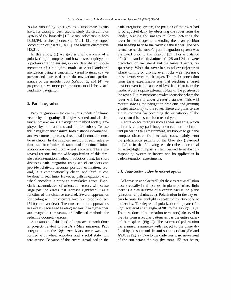
Whereas in unpolarized light the e-vector oscillationoccurs equally in all planes, in plane-polarized lightthere is a bias in favor of a certain oscillation plane(direction of polarization). Polarization in the sky oc-curs because the sunlight is scattered by atmosphericmolecules. The degree of polarization is greatest forlight scattered at an angle of 90◦ to the sunlight rays.The directions of polarization (e-vectors) observed inthe sky form a regular pattern across the entire celes-tial hemisphere (Fig. 2). The pattern of polarizationhas a mirror symmetry with respect to the plane de-fined by the solar and the anti-solar meridian (SM andASM in Fig. 2). Due to the daily westward movementof the sun across the sky (by some 15◦ per hour),
42 D. Lambrinos et al. / Robotics and Autonomous Systems 30 (2000) 39–64
Fig. 2. 3-D representation of the pattern of polarization in thesky as experienced by an observer in point O. Orientation andwidth of the bars depict the direction and degree of polarization,respectively. A prominent property of the pattern is a symmetryline running through sun (S) and zenith (Z), called “solar meridian”(SM) on the side of the sun and “anti-solar meridian” (ASM) onthe opposite side. Adapted from [46].
the symmetry plane, and with it the whole e-vectorpattern, rotates about the zenith. The pattern retainstwo important characteristics over the day: its mirrorsymmetry, and the property that along the symmetryline the e-vectors are always perpendicular to the solarmeridian.
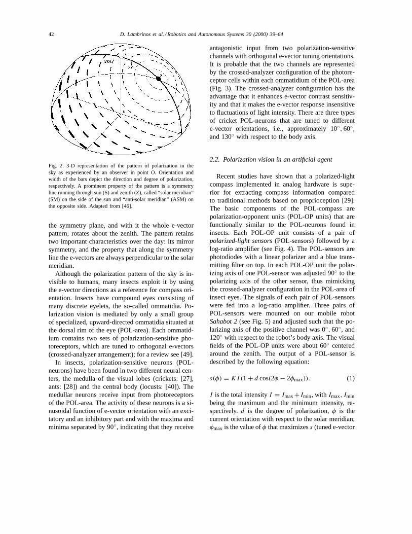
Although the polarization pattern of the sky is in-visible to humans, many insects exploit it by usingthe e-vector directions as a reference for compass ori-entation. Insects have compound eyes consisting ofmany discrete eyelets, the so-called ommatidia. Po-larization vision is mediated by only a small groupof specialized, upward-directed ommatidia situated atthe dorsal rim of the eye (POL-area). Each ommatid-ium contains two sets of polarization-sensitive pho-toreceptors, which are tuned to orthogonal e-vectors(crossed-analyzer arrangement); for a review see [49].
In insects, polarization-sensitive neurons (POL-neurons) have been found in two different neural cen-ters, the medulla of the visual lobes (crickets: [27],ants: [28]) and the central body (locusts: [40]). Themedullar neurons receive input from photoreceptorsof the POL-area. The activity of these neurons is a si-nusoidal function of e-vector orientation with an exci-tatory and an inhibitory part and with the maxima andminima separated by 90◦, indicating that they receive
antagonistic input from two polarization-sensitivechannels with orthogonal e-vector tuning orientations.It is probable that the two channels are representedby the crossed-analyzer configuration of the photore-ceptor cells within each ommatidium of the POL-area(Fig. 3). The crossed-analyzer configuration has theadvantage that it enhances e-vector contrast sensitiv-ity and that it makes the e-vector response insensitiveto fluctuations of light intensity. There are three typesof cricket POL-neurons that are tuned to differente-vector orientations, i.e., approximately 10◦, 60◦,and 130◦ with respect to the body axis.
2.2. Polarization vision in an artificial agent
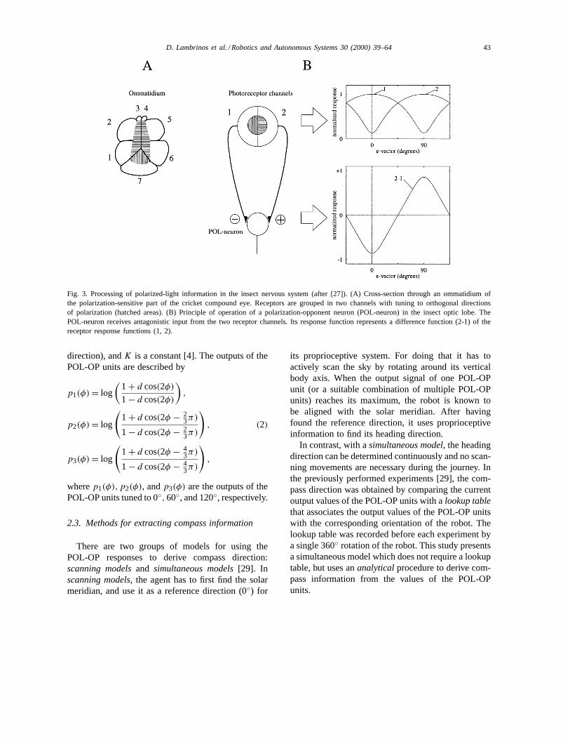
Recent studies have shown that a polarized-lightcompass implemented in analog hardware is supe-rior for extracting compass information comparedto traditional methods based on proprioception [29].The basic components of the POL-compass arepolarization-opponent units (POL-OP units) that arefunctionally similar to the POL-neurons found ininsects. Each POL-OP unit consists of a pair ofpolarized-light sensors(POL-sensors) followed by alog-ratio amplifier (see Fig. 4). The POL-sensors arephotodiodes with a linear polarizer and a blue trans-mitting filter on top. In each POL-OP unit the polar-izing axis of one POL-sensor was adjusted 90◦ to thepolarizing axis of the other sensor, thus mimickingthe crossed-analyzer configuration in the POL-area ofinsect eyes. The signals of each pair of POL-sensorswere fed into a log-ratio amplifier. Three pairs ofPOL-sensors were mounted on our mobile robotSahabot 2(see Fig. 5) and adjusted such that the po-larizing axis of the positive channel was 0◦, 60◦, and120◦ with respect to the robot’s body axis. The visualfields of the POL-OP units were about 60◦ centeredaround the zenith. The output of a POL-sensor isdescribed by the following equation:
s(φ) = KI (1 + d cos(2φ − 2φmax)). (1)
I is the total intensityI = Imax+Imin, with Imax, Iminbeing the maximum and the minimum intensity, re-spectively.d is the degree of polarization,φ is thecurrent orientation with respect to the solar meridian,φmax is the value ofφ that maximizess (tuned e-vector
D. Lambrinos et al. / Robotics and Autonomous Systems 30 (2000) 39–64 43
Fig. 3. Processing of polarized-light information in the insect nervous system (after [27]). (A) Cross-section through an ommatidium ofthe polarization-sensitive part of the cricket compound eye. Receptors are grouped in two channels with tuning to orthogonal directionsof polarization (hatched areas). (B) Principle of operation of a polarization-opponent neuron (POL-neuron) in the insect optic lobe. ThePOL-neuron receives antagonistic input from the two receptor channels. Its response function represents a difference function (2-1) of thereceptor response functions (1, 2).
direction), andK is a constant [4]. The outputs of thePOL-OP units are described by
p1(φ) = log
(1 + d cos(2φ)
1 − d cos(2φ)
),
p2(φ) = log
(1 + d cos(2φ − 2
3π)
1 − d cos(2φ − 23π)
), (2)
p3(φ) = log
(1 + d cos(2φ − 4
3π)
1 − d cos(2φ − 43π)
),
wherep1(φ), p2(φ), andp3(φ) are the outputs of thePOL-OP units tuned to 0◦, 60◦, and 120◦, respectively.
2.3. Methods for extracting compass information
There are two groups of models for using thePOL-OP responses to derive compass direction:scanning modelsand simultaneous models[29]. Inscanning models, the agent has to first find the solarmeridian, and use it as a reference direction (0◦) for
its proprioceptive system. For doing that it has toactively scan the sky by rotating around its verticalbody axis. When the output signal of one POL-OPunit (or a suitable combination of multiple POL-OPunits) reaches its maximum, the robot is known tobe aligned with the solar meridian. After havingfound the reference direction, it uses proprioceptiveinformation to find its heading direction.
In contrast, with asimultaneous model, the headingdirection can be determined continuously and no scan-ning movements are necessary during the journey. Inthe previously performed experiments [29], the com-pass direction was obtained by comparing the currentoutput values of the POL-OP units with alookup tablethat associates the output values of the POL-OP unitswith the corresponding orientation of the robot. Thelookup table was recorded before each experiment bya single 360◦ rotation of the robot. This study presentsa simultaneous model which does not require a lookuptable, but uses ananalyticalprocedure to derive com-pass information from the values of the POL-OPunits.
44 D. Lambrinos et al. / Robotics and Autonomous Systems 30 (2000) 39–64
Fig. 4. Diagrammatic description of a polarization-opponent unit (POL-OP unit). A POL-OP unit consists of a pair of POL-sensors anda log-ratio amplifier. The log-ratio amplifier receives input from the two POL-sensors and delivers the difference of their logarithmizedsignals. The e-vector responses of the POL-sensors (1, 2) follow a cos2-function.
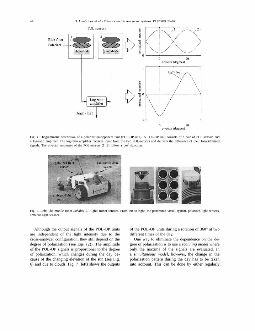
Fig. 5. Left: The mobile robotSahabot 2. Right: Robot sensors. From left to right: the panoramic visual system, polarized-light sensors,ambient-light sensors.
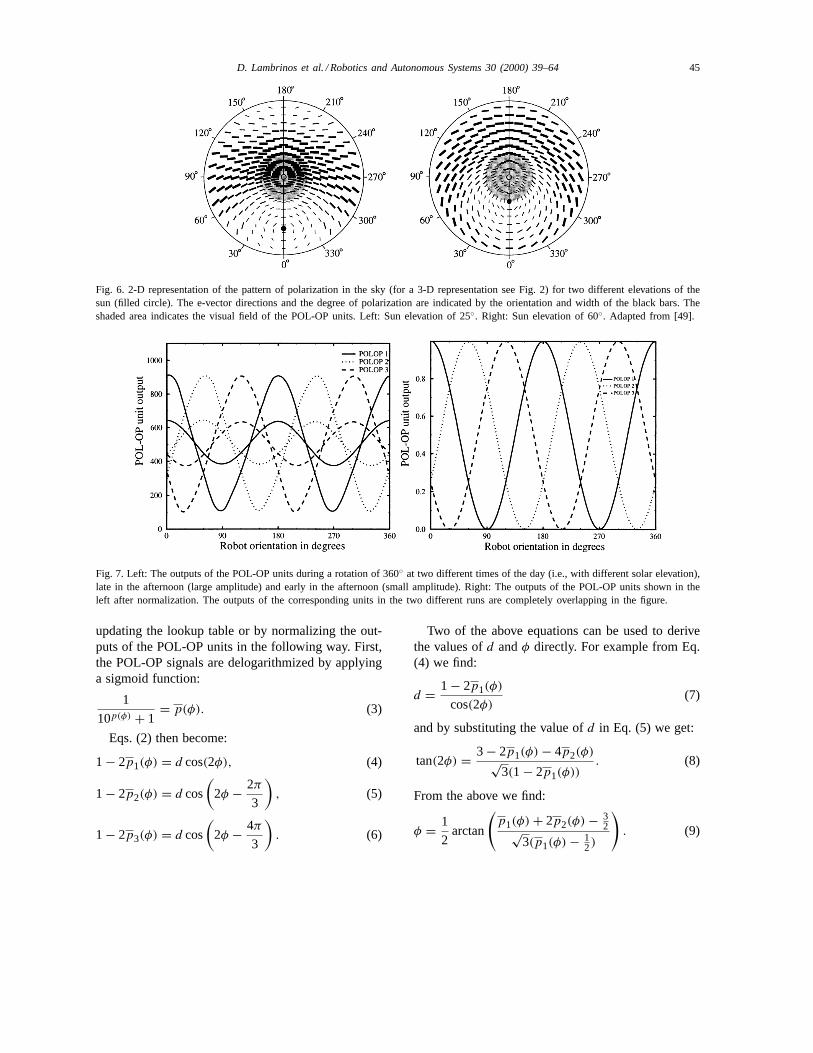
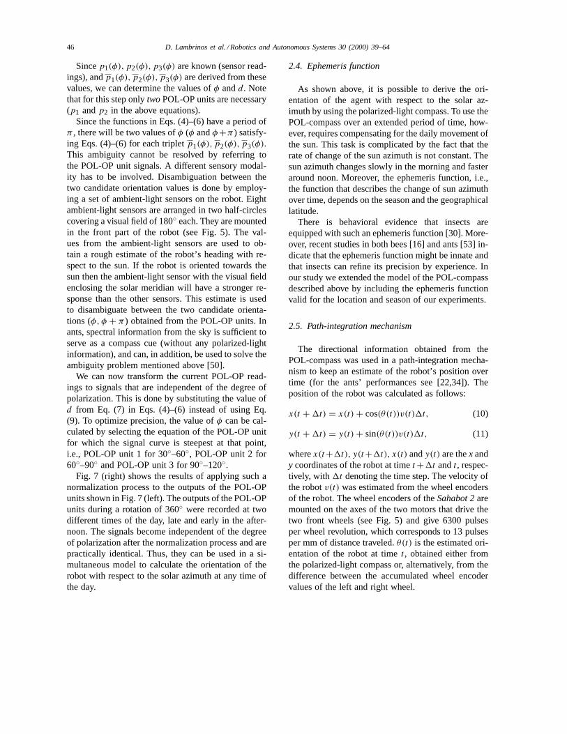
Although the output signals of the POL-OP unitsare independent of the light intensity due to thecross-analyzer configuration, they still depend on thedegree of polarization (see Eqs. (2)). The amplitudeof the POL-OP signals is proportional to the degreeof polarization, which changes during the day be-cause of the changing elevation of the sun (see Fig.6) and due to clouds. Fig. 7 (left) shows the outputs
of the POL-OP units during a rotation of 360◦ at twodifferent times of the day.
One way to eliminate the dependence on the de-gree of polarization is to use ascanning modelwhereonly the maxima of the signals are evaluated. Ina simultaneous model, however, the change in thepolarization pattern during the day has to be takeninto account. This can be done by either regularly
D. Lambrinos et al. / Robotics and Autonomous Systems 30 (2000) 39–64 45
Fig. 6. 2-D representation of the pattern of polarization in the sky (for a 3-D representation see Fig. 2) for two different elevations of thesun (filled circle). The e-vector directions and the degree of polarization are indicated by the orientation and width of the black bars. Theshaded area indicates the visual field of the POL-OP units. Left: Sun elevation of 25◦. Right: Sun elevation of 60◦. Adapted from [49].
Fig. 7. Left: The outputs of the POL-OP units during a rotation of 360◦ at two different times of the day (i.e., with different solar elevation),late in the afternoon (large amplitude) and early in the afternoon (small amplitude). Right: The outputs of the POL-OP units shown in theleft after normalization. The outputs of the corresponding units in the two different runs are completely overlapping in the figure.
updating the lookup table or by normalizing the out-puts of the POL-OP units in the following way. First,the POL-OP signals are delogarithmized by applyinga sigmoid function:
1
10p(φ) + 1= p(φ). (3)
Eqs. (2) then become:
1 − 2p1(φ) = d cos(2φ), (4)
1 − 2p2(φ) = d cos
(2φ − 2π
3
), (5)
1 − 2p3(φ) = d cos
(2φ − 4π
3
). (6)
Two of the above equations can be used to derivethe values ofd andφ directly. For example from Eq.(4) we find:
d = 1 − 2p1(φ)
cos(2φ)(7)
and by substituting the value ofd in Eq. (5) we get:
tan(2φ) = 3 − 2p1(φ) − 4p2(φ)√3(1 − 2p1(φ))
. (8)
From the above we find:
φ = 1
2arctan
(p1(φ) + 2p2(φ) − 3
2√3(p1(φ) − 1
2)
). (9)
46 D. Lambrinos et al. / Robotics and Autonomous Systems 30 (2000) 39–64
Sincep1(φ), p2(φ), p3(φ) are known (sensor read-ings), andp1(φ), p2(φ), p3(φ) are derived from thesevalues, we can determine the values ofφ andd. Notethat for this step onlytwoPOL-OP units are necessary(p1 andp2 in the above equations).
Since the functions in Eqs. (4)–(6) have a period ofπ , there will be two values ofφ (φ andφ+π ) satisfy-ing Eqs. (4)–(6) for each tripletp1(φ), p2(φ), p3(φ).This ambiguity cannot be resolved by referring tothe POL-OP unit signals. A different sensory modal-ity has to be involved. Disambiguation between thetwo candidate orientation values is done by employ-ing a set of ambient-light sensors on the robot. Eightambient-light sensors are arranged in two half-circlescovering a visual field of 180◦ each. They are mountedin the front part of the robot (see Fig. 5). The val-ues from the ambient-light sensors are used to ob-tain a rough estimate of the robot’s heading with re-spect to the sun. If the robot is oriented towards thesun then the ambient-light sensor with the visual fieldenclosing the solar meridian will have a stronger re-sponse than the other sensors. This estimate is usedto disambiguate between the two candidate orienta-tions (φ, φ + π ) obtained from the POL-OP units. Inants, spectral information from the sky is sufficient toserve as a compass cue (without any polarized-lightinformation), and can, in addition, be used to solve theambiguity problem mentioned above [50].
We can now transform the current POL-OP read-ings to signals that are independent of the degree ofpolarization. This is done by substituting the value ofd from Eq. (7) in Eqs. (4)–(6) instead of using Eq.(9). To optimize precision, the value ofφ can be cal-culated by selecting the equation of the POL-OP unitfor which the signal curve is steepest at that point,i.e., POL-OP unit 1 for 30◦–60◦, POL-OP unit 2 for60◦–90◦ and POL-OP unit 3 for 90◦–120◦.
Fig. 7 (right) shows the results of applying such anormalization process to the outputs of the POL-OPunits shown in Fig. 7 (left). The outputs of the POL-OPunits during a rotation of 360◦ were recorded at twodifferent times of the day, late and early in the after-noon. The signals become independent of the degreeof polarization after the normalization process and arepractically identical. Thus, they can be used in a si-multaneous model to calculate the orientation of therobot with respect to the solar azimuth at any time ofthe day.
2.4. Ephemeris function
As shown above, it is possible to derive the ori-entation of the agent with respect to the solar az-imuth by using the polarized-light compass. To use thePOL-compass over an extended period of time, how-ever, requires compensating for the daily movement ofthe sun. This task is complicated by the fact that therate of change of the sun azimuth is not constant. Thesun azimuth changes slowly in the morning and fasteraround noon. Moreover, the ephemeris function, i.e.,the function that describes the change of sun azimuthover time, depends on the season and the geographicallatitude.
There is behavioral evidence that insects areequipped with such an ephemeris function [30]. More-over, recent studies in both bees [16] and ants [53] in-dicate that the ephemeris function might be innate andthat insects can refine its precision by experience. Inour study we extended the model of the POL-compassdescribed above by including the ephemeris functionvalid for the location and season of our experiments.
2.5. Path-integration mechanism
The directional information obtained from thePOL-compass was used in a path-integration mecha-nism to keep an estimate of the robot’s position overtime (for the ants’ performances see [22,34]). Theposition of the robot was calculated as follows:
x(t + 1t) = x(t) + cos(θ(t))v(t)1t, (10)
y(t + 1t) = y(t) + sin(θ(t))v(t)1t, (11)
wherex(t+1t), y(t+1t), x(t) andy(t) are thex andy coordinates of the robot at timet +1t andt , respec-tively, with 1t denoting the time step. The velocity ofthe robotv(t) was estimated from the wheel encodersof the robot. The wheel encoders of theSahabot 2aremounted on the axes of the two motors that drive thetwo front wheels (see Fig. 5) and give 6300 pulsesper wheel revolution, which corresponds to 13 pulsesper mm of distance traveled.θ(t) is the estimated ori-entation of the robot at timet , obtained either fromthe polarized-light compass or, alternatively, from thedifference between the accumulated wheel encodervalues of the left and right wheel.
D. Lambrinos et al. / Robotics and Autonomous Systems 30 (2000) 39–64 47
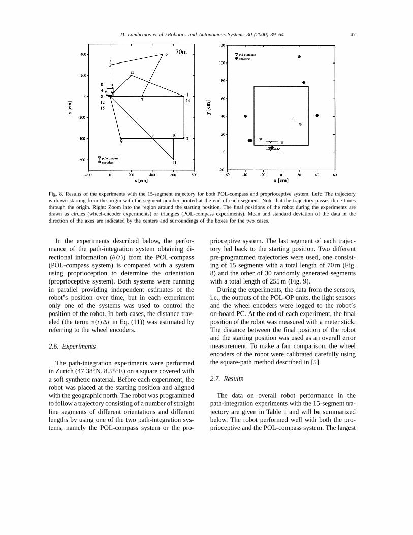
Fig. 8. Results of the experiments with the 15-segment trajectory for both POL-compass and proprioceptive system. Left: The trajectoryis drawn starting from the origin with the segment number printed at the end of each segment. Note that the trajectory passes three timesthrough the origin. Right: Zoom into the region around the starting position. The final positions of the robot during the experiments aredrawn as circles (wheel-encoder experiments) or triangles (POL-compass experiments). Mean and standard deviation of the data in thedirection of the axes are indicated by the centers and surroundings of the boxes for the two cases.
In the experiments described below, the perfor-mance of the path-integration system obtaining di-rectional information (θ(t)) from the POL-compass(POL-compass system) is compared with a systemusing proprioception to determine the orientation(proprioceptive system). Both systems were runningin parallel providing independent estimates of therobot’s position over time, but in each experimentonly one of the systems was used to control theposition of the robot. In both cases, the distance trav-eled (the term:v(t)1t in Eq. (11)) was estimated byreferring to the wheel encoders.
2.6. Experiments
The path-integration experiments were performedin Zurich (47.38◦N, 8.55◦E) on a square covered witha soft synthetic material. Before each experiment, therobot was placed at the starting position and alignedwith the geographic north. The robot was programmedto follow a trajectory consisting of a number of straightline segments of different orientations and differentlengths by using one of the two path-integration sys-tems, namely the POL-compass system or the pro-
prioceptive system. The last segment of each trajec-tory led back to the starting position. Two differentpre-programmed trajectories were used, one consist-ing of 15 segments with a total length of 70 m (Fig.8) and the other of 30 randomly generated segmentswith a total length of 255 m (Fig. 9).
During the experiments, the data from the sensors,i.e., the outputs of the POL-OP units, the light sensorsand the wheel encoders were logged to the robot’son-board PC. At the end of each experiment, the finalposition of the robot was measured with a meter stick.The distance between the final position of the robotand the starting position was used as an overall errormeasurement. To make a fair comparison, the wheelencoders of the robot were calibrated carefully usingthe square-path method described in [5].
2.7. Results
The data on overall robot performance in thepath-integration experiments with the 15-segment tra-jectory are given in Table 1 and will be summarizedbelow. The robot performed well with both the pro-prioceptive and the POL-compass system. The largest
48 D. Lambrinos et al. / Robotics and Autonomous Systems 30 (2000) 39–64
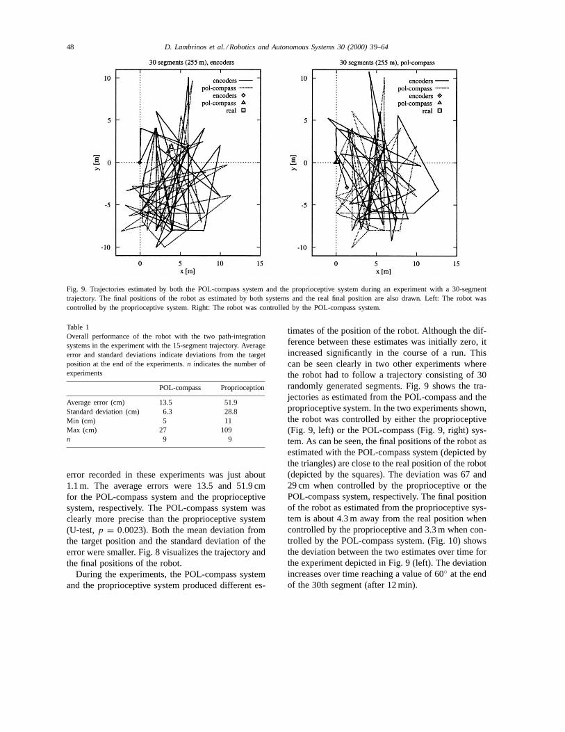
Fig. 9. Trajectories estimated by both the POL-compass system and the proprioceptive system during an experiment with a 30-segmenttrajectory. The final positions of the robot as estimated by both systems and the real final position are also drawn. Left: The robot wascontrolled by the proprioceptive system. Right: The robot was controlled by the POL-compass system.
Table 1Overall performance of the robot with the two path-integrationsystems in the experiment with the 15-segment trajectory. Averageerror and standard deviations indicate deviations from the targetposition at the end of the experiments.n indicates the number ofexperiments
POL-compass Proprioception
Average error (cm) 13.5 51.9Standard deviation (cm) 6.3 28.8Min (cm) 5 11Max (cm) 27 109n 9 9
error recorded in these experiments was just about1.1 m. The average errors were 13.5 and 51.9 cmfor the POL-compass system and the proprioceptivesystem, respectively. The POL-compass system wasclearly more precise than the proprioceptive system(U-test,p = 0.0023). Both the mean deviation fromthe target position and the standard deviation of theerror were smaller. Fig. 8 visualizes the trajectory andthe final positions of the robot.
During the experiments, the POL-compass systemand the proprioceptive system produced different es-
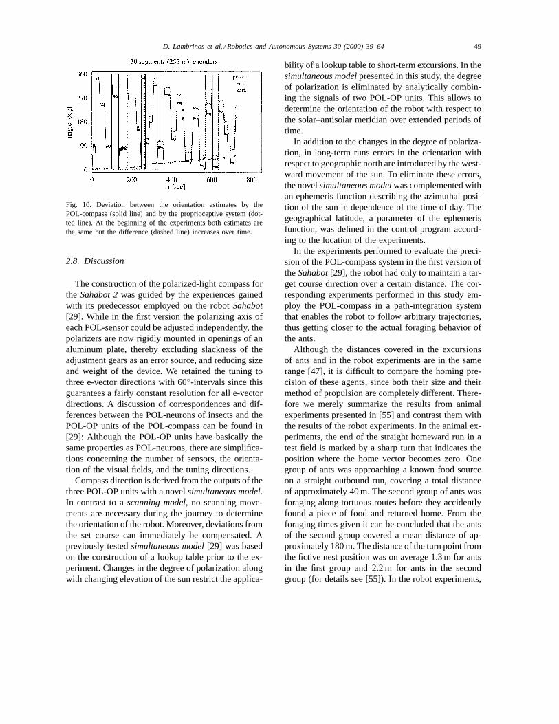
timates of the position of the robot. Although the dif-ference between these estimates was initially zero, itincreased significantly in the course of a run. Thiscan be seen clearly in two other experiments wherethe robot had to follow a trajectory consisting of 30randomly generated segments. Fig. 9 shows the tra-jectories as estimated from the POL-compass and theproprioceptive system. In the two experiments shown,the robot was controlled by either the proprioceptive(Fig. 9, left) or the POL-compass (Fig. 9, right) sys-tem. As can be seen, the final positions of the robot asestimated with the POL-compass system (depicted bythe triangles) are close to the real position of the robot(depicted by the squares). The deviation was 67 and29 cm when controlled by the proprioceptive or thePOL-compass system, respectively. The final positionof the robot as estimated from the proprioceptive sys-tem is about 4.3 m away from the real position whencontrolled by the proprioceptive and 3.3 m when con-trolled by the POL-compass system. (Fig. 10) showsthe deviation between the two estimates over time forthe experiment depicted in Fig. 9 (left). The deviationincreases over time reaching a value of 60◦ at the endof the 30th segment (after 12 min).
D. Lambrinos et al. / Robotics and Autonomous Systems 30 (2000) 39–64 49
Fig. 10. Deviation between the orientation estimates by thePOL-compass (solid line) and by the proprioceptive system (dot-ted line). At the beginning of the experiments both estimates arethe same but the difference (dashed line) increases over time.
2.8. Discussion
The construction of the polarized-light compass forthe Sahabot 2was guided by the experiences gainedwith its predecessor employed on the robotSahabot[29]. While in the first version the polarizing axis ofeach POL-sensor could be adjusted independently, thepolarizers are now rigidly mounted in openings of analuminum plate, thereby excluding slackness of theadjustment gears as an error source, and reducing sizeand weight of the device. We retained the tuning tothree e-vector directions with 60◦-intervals since thisguarantees a fairly constant resolution for all e-vectordirections. A discussion of correspondences and dif-ferences between the POL-neurons of insects and thePOL-OP units of the POL-compass can be found in[29]: Although the POL-OP units have basically thesame properties as POL-neurons, there are simplifica-tions concerning the number of sensors, the orienta-tion of the visual fields, and the tuning directions.
Compass direction is derived from the outputs of thethree POL-OP units with a novelsimultaneous model.In contrast to ascanning model, no scanning move-ments are necessary during the journey to determinethe orientation of the robot. Moreover, deviations fromthe set course can immediately be compensated. Apreviously testedsimultaneous model[29] was basedon the construction of a lookup table prior to the ex-periment. Changes in the degree of polarization alongwith changing elevation of the sun restrict the applica-
bility of a lookup table to short-term excursions. In thesimultaneous modelpresented in this study, the degreeof polarization is eliminated by analytically combin-ing the signals of two POL-OP units. This allows todetermine the orientation of the robot with respect tothe solar–antisolar meridian over extended periods oftime.
In addition to the changes in the degree of polariza-tion, in long-term runs errors in the orientation withrespect to geographic north are introduced by the west-ward movement of the sun. To eliminate these errors,the novelsimultaneous modelwas complemented withan ephemeris function describing the azimuthal posi-tion of the sun in dependence of the time of day. Thegeographical latitude, a parameter of the ephemerisfunction, was defined in the control program accord-ing to the location of the experiments.
In the experiments performed to evaluate the preci-sion of the POL-compass system in the first version oftheSahabot[29], the robot had only to maintain a tar-get course direction over a certain distance. The cor-responding experiments performed in this study em-ploy the POL-compass in a path-integration systemthat enables the robot to follow arbitrary trajectories,thus getting closer to the actual foraging behavior ofthe ants.
Although the distances covered in the excursionsof ants and in the robot experiments are in the samerange [47], it is difficult to compare the homing pre-cision of these agents, since both their size and theirmethod of propulsion are completely different. There-fore we merely summarize the results from animalexperiments presented in [55] and contrast them withthe results of the robot experiments. In the animal ex-periments, the end of the straight homeward run in atest field is marked by a sharp turn that indicates theposition where the home vector becomes zero. Onegroup of ants was approaching a known food sourceon a straight outbound run, covering a total distanceof approximately 40 m. The second group of ants wasforaging along tortuous routes before they accidentlyfound a piece of food and returned home. From theforaging times given it can be concluded that the antsof the second group covered a mean distance of ap-proximately 180 m. The distance of the turn point fromthe fictive nest position was on average 1.3 m for antsin the first group and 2.2 m for ants in the secondgroup (for details see [55]). In the robot experiments,
50 D. Lambrinos et al. / Robotics and Autonomous Systems 30 (2000) 39–64
the mean error amounted to 13 cm for a path lengthof approximately 70 m when using the POL-compass.For the two 30-segment trajectories with a length of255 m estimated by the POL-compass system, errorsof 67 and 29 cm were recorded.
The precision of the POL-compass system can beevaluated by a comparison of a path-integration systemwhich derives orientation from the POL-compass withanother system where orientation is computed from acarefully calibrated proprioceptive system (wheel en-coders). Results obtained in experiments where therobot had to travel along a 15-segment trajectory witha total length of 70 m demonstrate that the standarddeviation of the final position error is by a factor ofapproximately 5 smaller in the POL-compass system(Table 1). The systematic deviation of the mean posi-tion that was observed for the POL-compass system isprobably caused by a slight inclination from the hor-izontal at the outer parts of the test field. This causesa shift of the visual field of the POL-OP units awayfrom the zenith where the pattern exhibits a mirrorsymmetry (see Fig. 6). Integration over the visual fieldwhich is not centered on the solar–antisolar meridianwill therefore result in a total e-vector which is notperpendicular to this meridian.
The use of an inertial navigation system forpath integration would be another alternative to theabove-mentioned methods. The advantage of inertialnavigation systems is that they are self-contained andcan provide very fast and dynamic measurements. Themain disadvantage of such a system is that it driftsover time, a fact that also makes a direct comparisonwith the POL-compass system difficult. A sophisti-cated and relatively cheap inertial navigation systemwas developed by Barshan and Durrant-Whyte [1,2]based on combinations of different solid-state gyros.They reported a typical error of 12◦ after 5 minutes(commercial, high-quality and expensive inertial nav-igation systems have a typical drift of about 2 kmafter 1 hour).
While the design of the POL-OP units closely corre-sponds to the e-vector detection system of insects, allcomponents of the path-integration system — the coreof thesimultaneous model(Section 2.3), the ephemerisfunction (Section 2.4), and the path-integration itself(Section 2.5) — are implemented in an analytical waywithout directly taking into account the specific pro-cessing capabilities of a neural substrate. It is, for
example, known that ants solve the path-integrationproblem not by performing true vector summation, butby employing an approximation, resulting in system-atic navigational errors under certain circumstances[34]. A neural model of the path-integration processwas proposed in [22], but neurophysiological or neu-roanatomical data are not available so far. Besides this,the experiments with path integration were conductedin order to evaluate the precision of the POL-compasssystem, which would have been more complicated byusing the approximative procedures that animals resortto or by implementing plausible neural models. Tak-ing the analytical models — which have been demon-strated to give the desired results — as a starting point,corresponding neural models could be derived.
3. Visual piloting
While path integration employing a skylight com-pass is the primary strategy thatCataglyphisants areusing to return to the vicinity of their nest, errors in-troduced by the path-integration process would resultin a wrong estimate of the nest position [55]. Since thenest entrance is an inconspicuous hole in the desertground (see Fig. 11) which is invisible to the insecteven from a small distance, alternative strategies haveto be employed in order to finally locate the entrance.
3.1. Visual piloting in natural agents
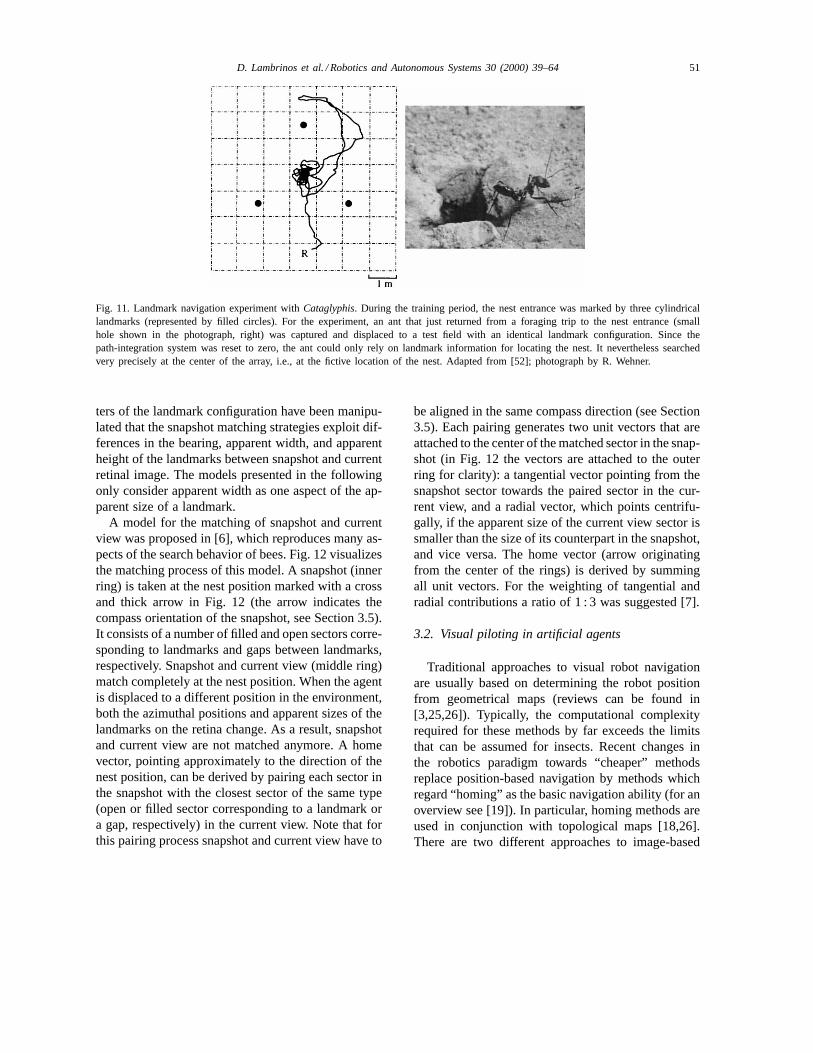
In the absence of visual landmarks,Cataglyphiswill start a systematic search at the position where thenest is expected after having reset its path-integrationsystem [51]. However, when landmark information isavailable, both bees [6] and ants [52] will exploit it,and they will relocate the target position directly witha remarkable precision (see Fig. 11).
A number of experiments performed with bees [6]and ants [52,54] have unveiled important propertiesof the insect’s landmark navigation system. The mainconclusion from these experiments is that the ani-mal stores a rather unprocessed visual snapshot of thescene around the goal position. By matching this snap-shot to the current retinal image, the insect can derivethe direction it has to move in order to relocate thetarget position where the snapshot was taken. There isevidence from experiments in which several parame-
D. Lambrinos et al. / Robotics and Autonomous Systems 30 (2000) 39–64 51
Fig. 11. Landmark navigation experiment withCataglyphis. During the training period, the nest entrance was marked by three cylindricallandmarks (represented by filled circles). For the experiment, an ant that just returned from a foraging trip to the nest entrance (smallhole shown in the photograph, right) was captured and displaced to a test field with an identical landmark configuration. Since thepath-integration system was reset to zero, the ant could only rely on landmark information for locating the nest. It nevertheless searchedvery precisely at the center of the array, i.e., at the fictive location of the nest. Adapted from [52]; photograph by R. Wehner.
ters of the landmark configuration have been manipu-lated that the snapshot matching strategies exploit dif-ferences in the bearing, apparent width, and apparentheight of the landmarks between snapshot and currentretinal image. The models presented in the followingonly consider apparent width as one aspect of the ap-parent size of a landmark.
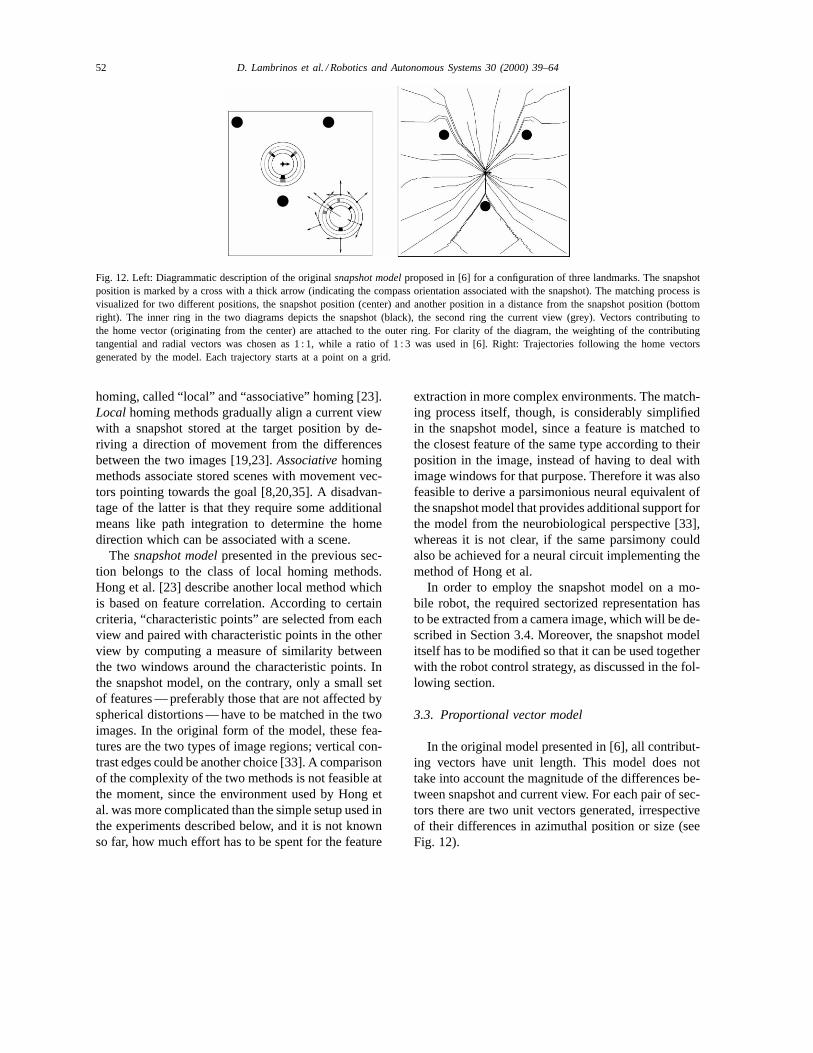
A model for the matching of snapshot and currentview was proposed in [6], which reproduces many as-pects of the search behavior of bees. Fig. 12 visualizesthe matching process of this model. A snapshot (innerring) is taken at the nest position marked with a crossand thick arrow in Fig. 12 (the arrow indicates thecompass orientation of the snapshot, see Section 3.5).It consists of a number of filled and open sectors corre-sponding to landmarks and gaps between landmarks,respectively. Snapshot and current view (middle ring)match completely at the nest position. When the agentis displaced to a different position in the environment,both the azimuthal positions and apparent sizes of thelandmarks on the retina change. As a result, snapshotand current view are not matched anymore. A homevector, pointing approximately to the direction of thenest position, can be derived by pairing each sector inthe snapshot with the closest sector of the same type(open or filled sector corresponding to a landmark ora gap, respectively) in the current view. Note that forthis pairing process snapshot and current view have to
be aligned in the same compass direction (see Section3.5). Each pairing generates two unit vectors that areattached to the center of the matched sector in the snap-shot (in Fig. 12 the vectors are attached to the outerring for clarity): a tangential vector pointing from thesnapshot sector towards the paired sector in the cur-rent view, and a radial vector, which points centrifu-gally, if the apparent size of the current view sector issmaller than the size of its counterpart in the snapshot,and vice versa. The home vector (arrow originatingfrom the center of the rings) is derived by summingall unit vectors. For the weighting of tangential andradial contributions a ratio of 1 : 3 was suggested [7].
3.2. Visual piloting in artificial agents
Traditional approaches to visual robot navigationare usually based on determining the robot positionfrom geometrical maps (reviews can be found in[3,25,26]). Typically, the computational complexityrequired for these methods by far exceeds the limitsthat can be assumed for insects. Recent changes inthe robotics paradigm towards “cheaper” methodsreplace position-based navigation by methods whichregard “homing” as the basic navigation ability (for anoverview see [19]). In particular, homing methods areused in conjunction with topological maps [18,26].There are two different approaches to image-based
52 D. Lambrinos et al. / Robotics and Autonomous Systems 30 (2000) 39–64
Fig. 12. Left: Diagrammatic description of the originalsnapshot modelproposed in [6] for a configuration of three landmarks. The snapshotposition is marked by a cross with a thick arrow (indicating the compass orientation associated with the snapshot). The matching process isvisualized for two different positions, the snapshot position (center) and another position in a distance from the snapshot position (bottomright). The inner ring in the two diagrams depicts the snapshot (black), the second ring the current view (grey). Vectors contributing tothe home vector (originating from the center) are attached to the outer ring. For clarity of the diagram, the weighting of the contributingtangential and radial vectors was chosen as 1 : 1, while a ratio of 1 : 3 was used in [6]. Right: Trajectories following the home vectorsgenerated by the model. Each trajectory starts at a point on a grid.
homing, called “local” and “associative” homing [23].Local homing methods gradually align a current viewwith a snapshot stored at the target position by de-riving a direction of movement from the differencesbetween the two images [19,23].Associativehomingmethods associate stored scenes with movement vec-tors pointing towards the goal [8,20,35]. A disadvan-tage of the latter is that they require some additionalmeans like path integration to determine the homedirection which can be associated with a scene.
The snapshot modelpresented in the previous sec-tion belongs to the class of local homing methods.Hong et al. [23] describe another local method whichis based on feature correlation. According to certaincriteria, “characteristic points” are selected from eachview and paired with characteristic points in the otherview by computing a measure of similarity betweenthe two windows around the characteristic points. Inthe snapshot model, on the contrary, only a small setof features — preferably those that are not affected byspherical distortions — have to be matched in the twoimages. In the original form of the model, these fea-tures are the two types of image regions; vertical con-trast edges could be another choice [33]. A comparisonof the complexity of the two methods is not feasible atthe moment, since the environment used by Hong etal. was more complicated than the simple setup used inthe experiments described below, and it is not knownso far, how much effort has to be spent for the feature
extraction in more complex environments. The match-ing process itself, though, is considerably simplifiedin the snapshot model, since a feature is matched tothe closest feature of the same type according to theirposition in the image, instead of having to deal withimage windows for that purpose. Therefore it was alsofeasible to derive a parsimonious neural equivalent ofthe snapshot model that provides additional support forthe model from the neurobiological perspective [33],whereas it is not clear, if the same parsimony couldalso be achieved for a neural circuit implementing themethod of Hong et al.
In order to employ the snapshot model on a mo-bile robot, the required sectorized representation hasto be extracted from a camera image, which will be de-scribed in Section 3.4. Moreover, the snapshot modelitself has to be modified so that it can be used togetherwith the robot control strategy, as discussed in the fol-lowing section.
3.3. Proportional vector model
In the original model presented in [6], all contribut-ing vectors have unit length. This model does nottake into account the magnitude of the differences be-tween snapshot and current view. For each pair of sec-tors there are two unit vectors generated, irrespectiveof their differences in azimuthal position or size (seeFig. 12).
D. Lambrinos et al. / Robotics and Autonomous Systems 30 (2000) 39–64 53
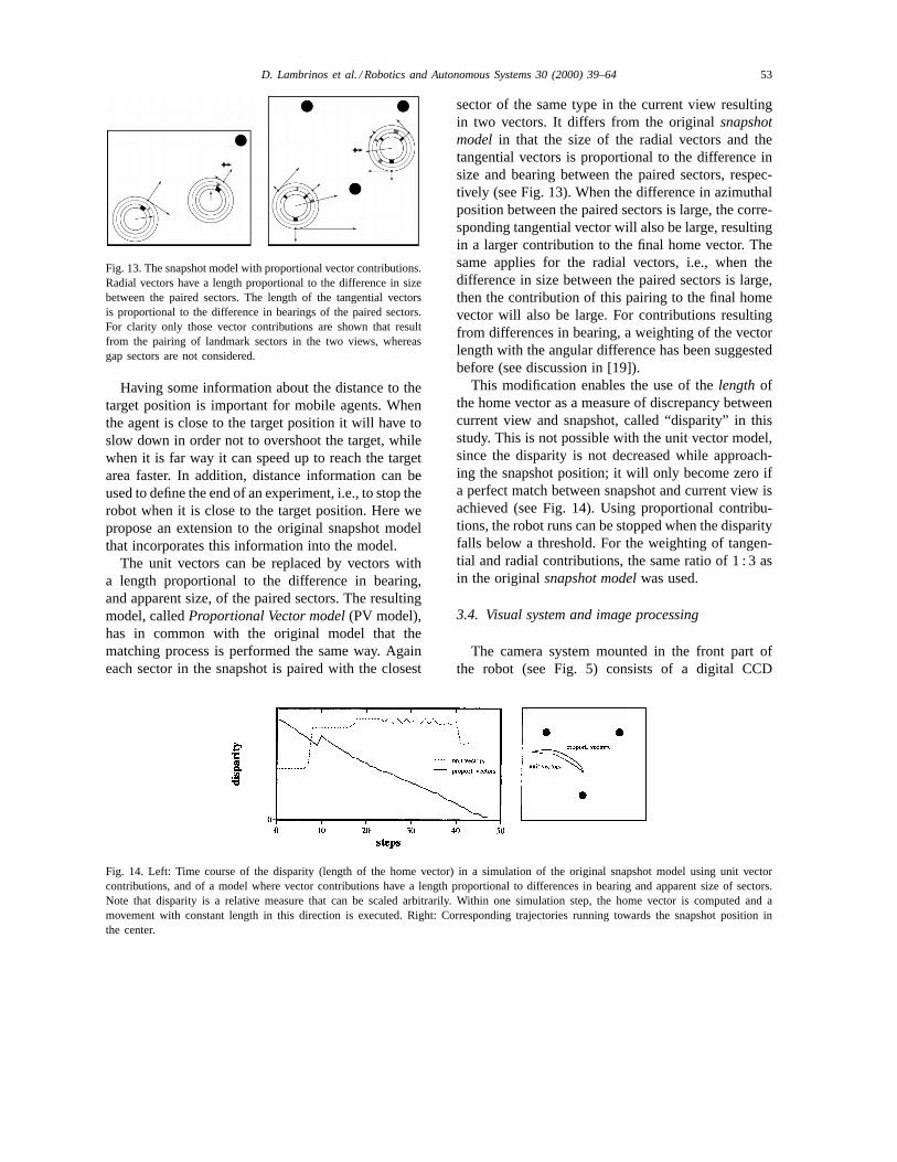
Fig. 13. The snapshot model with proportional vector contributions.Radial vectors have a length proportional to the difference in sizebetween the paired sectors. The length of the tangential vectorsis proportional to the difference in bearings of the paired sectors.For clarity only those vector contributions are shown that resultfrom the pairing of landmark sectors in the two views, whereasgap sectors are not considered.
Having some information about the distance to thetarget position is important for mobile agents. Whenthe agent is close to the target position it will have toslow down in order not to overshoot the target, whilewhen it is far way it can speed up to reach the targetarea faster. In addition, distance information can beused to define the end of an experiment, i.e., to stop therobot when it is close to the target position. Here wepropose an extension to the original snapshot modelthat incorporates this information into the model.
The unit vectors can be replaced by vectors witha length proportional to the difference in bearing,and apparent size, of the paired sectors. The resultingmodel, calledProportional Vector model(PV model),has in common with the original model that thematching process is performed the same way. Againeach sector in the snapshot is paired with the closest
Fig. 14. Left: Time course of the disparity (length of the home vector) in a simulation of the original snapshot model using unit vectorcontributions, and of a model where vector contributions have a length proportional to differences in bearing and apparent size of sectors.Note that disparity is a relative measure that can be scaled arbitrarily. Within one simulation step, the home vector is computed and amovement with constant length in this direction is executed. Right: Corresponding trajectories running towards the snapshot position inthe center.
sector of the same type in the current view resultingin two vectors. It differs from the originalsnapshotmodel in that the size of the radial vectors and thetangential vectors is proportional to the difference insize and bearing between the paired sectors, respec-tively (see Fig. 13). When the difference in azimuthalposition between the paired sectors is large, the corre-sponding tangential vector will also be large, resultingin a larger contribution to the final home vector. Thesame applies for the radial vectors, i.e., when thedifference in size between the paired sectors is large,then the contribution of this pairing to the final homevector will also be large. For contributions resultingfrom differences in bearing, a weighting of the vectorlength with the angular difference has been suggestedbefore (see discussion in [19]).
This modification enables the use of thelengthofthe home vector as a measure of discrepancy betweencurrent view and snapshot, called “disparity” in thisstudy. This is not possible with the unit vector model,since the disparity is not decreased while approach-ing the snapshot position; it will only become zero ifa perfect match between snapshot and current view isachieved (see Fig. 14). Using proportional contribu-tions, the robot runs can be stopped when the disparityfalls below a threshold. For the weighting of tangen-tial and radial contributions, the same ratio of 1 : 3 asin the originalsnapshot modelwas used.
3.4. Visual system and image processing
The camera system mounted in the front part ofthe robot (see Fig. 5) consists of a digital CCD
54 D. Lambrinos et al. / Robotics and Autonomous Systems 30 (2000) 39–64
camera and a conically shaped mirror in the ver-tical optical axis of the camera. The conical mir-ror was made of polished brass that went througha chrome-plating process to improve the opticalquality.
With the help of the conical mirror, a panoramic,360◦ view is obtained; a similar imaging techniquewas used in [9,19,39,57] (for a detailed descriptionsee [10]). When the axis of the cone coincides withthe optical axis of the camera, horizontal slices of theenvironment appear as concentric circles in the im-age. Special adjustment screws located at the base ofthe camera module were used for tuning the opticalaxis of the camera. In order to see the horizon, theopening angle of the cone was determined by con-sidering the visual field angle of the CCD camera. Inthe experiments described here, the opening angle ofthe cone was chosen so that the visual field extends±10◦ around the horizon. The whole camera modulewas mounted as low as possible on the robot withinthe construction constraints, which brings the mirrorto a height of approximately 27 cm above the ground.In order to reduce the total light intensity, a neutraldensity filter was mounted between camera and mir-ror. An additional infrared filter was necessary to pre-vent the influence of thermal radiation on the cameraimage.
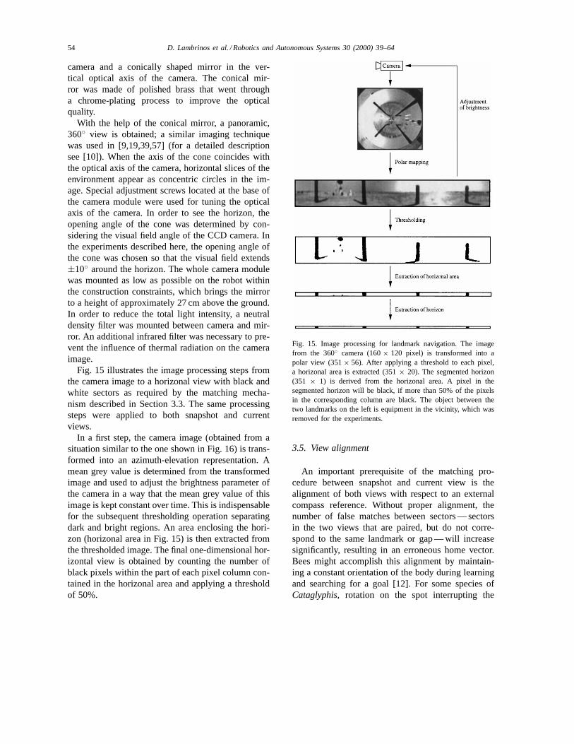
Fig. 15 illustrates the image processing steps fromthe camera image to a horizonal view with black andwhite sectors as required by the matching mecha-nism described in Section 3.3. The same processingsteps were applied to both snapshot and currentviews.
In a first step, the camera image (obtained from asituation similar to the one shown in Fig. 16) is trans-formed into an azimuth-elevation representation. Amean grey value is determined from the transformedimage and used to adjust the brightness parameter ofthe camera in a way that the mean grey value of thisimage is kept constant over time. This is indispensablefor the subsequent thresholding operation separatingdark and bright regions. An area enclosing the hori-zon (horizonal area in Fig. 15) is then extracted fromthe thresholded image. The final one-dimensional hor-izontal view is obtained by counting the number ofblack pixels within the part of each pixel column con-tained in the horizonal area and applying a thresholdof 50%.
Fig. 15. Image processing for landmark navigation. The imagefrom the 360◦ camera (160× 120 pixel) is transformed into apolar view (351× 56). After applying a threshold to each pixel,a horizonal area is extracted (351× 20). The segmented horizon(351 × 1) is derived from the horizonal area. A pixel in thesegmented horizon will be black, if more than 50% of the pixelsin the corresponding column are black. The object between thetwo landmarks on the left is equipment in the vicinity, which wasremoved for the experiments.
3.5. View alignment
An important prerequisite of the matching pro-cedure between snapshot and current view is thealignment of both views with respect to an externalcompass reference. Without proper alignment, thenumber of false matches between sectors — sectorsin the two views that are paired, but do not corre-spond to the same landmark or gap — will increasesignificantly, resulting in an erroneous home vector.Bees might accomplish this alignment by maintain-ing a constant orientation of the body during learningand searching for a goal [12]. For some species ofCataglyphis, rotation on the spot interrupting the
D. Lambrinos et al. / Robotics and Autonomous Systems 30 (2000) 39–64 55
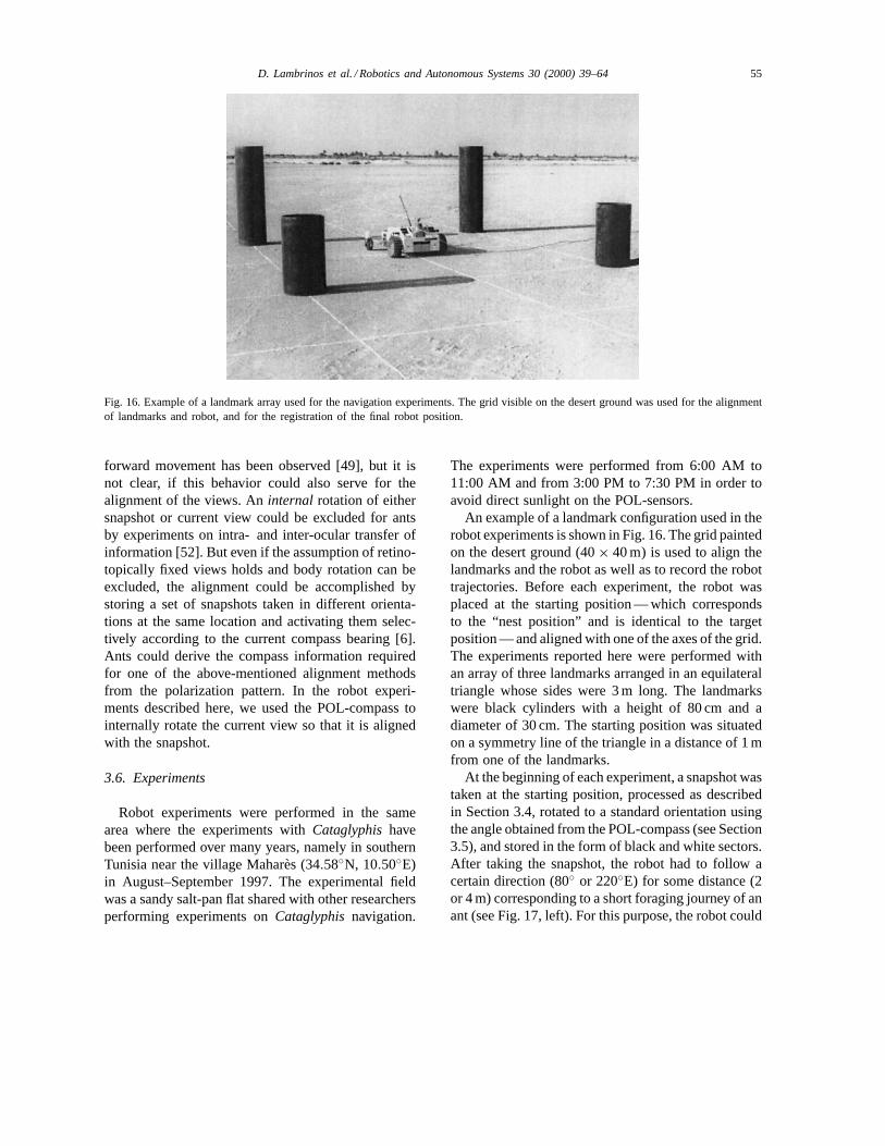
Fig. 16. Example of a landmark array used for the navigation experiments. The grid visible on the desert ground was used for the alignmentof landmarks and robot, and for the registration of the final robot position.
forward movement has been observed [49], but it isnot clear, if this behavior could also serve for thealignment of the views. Aninternal rotation of eithersnapshot or current view could be excluded for antsby experiments on intra- and inter-ocular transfer ofinformation [52]. But even if the assumption of retino-topically fixed views holds and body rotation can beexcluded, the alignment could be accomplished bystoring a set of snapshots taken in different orienta-tions at the same location and activating them selec-tively according to the current compass bearing [6].Ants could derive the compass information requiredfor one of the above-mentioned alignment methodsfrom the polarization pattern. In the robot experi-ments described here, we used the POL-compass tointernally rotate the current view so that it is alignedwith the snapshot.
3.6. Experiments
Robot experiments were performed in the samearea where the experiments withCataglyphishavebeen performed over many years, namely in southernTunisia near the village Maharès (34.58◦N, 10.50◦E)in August–September 1997. The experimental fieldwas a sandy salt-pan flat shared with other researchersperforming experiments onCataglyphisnavigation.
The experiments were performed from 6:00 AM to11:00 AM and from 3:00 PM to 7:30 PM in order toavoid direct sunlight on the POL-sensors.
An example of a landmark configuration used in therobot experiments is shown in Fig. 16. The grid paintedon the desert ground (40× 40 m) is used to align thelandmarks and the robot as well as to record the robottrajectories. Before each experiment, the robot wasplaced at the starting position — which correspondsto the “nest position” and is identical to the targetposition — and aligned with one of the axes of the grid.The experiments reported here were performed withan array of three landmarks arranged in an equilateraltriangle whose sides were 3 m long. The landmarkswere black cylinders with a height of 80 cm and adiameter of 30 cm. The starting position was situatedon a symmetry line of the triangle in a distance of 1 mfrom one of the landmarks.
At the beginning of each experiment, a snapshot wastaken at the starting position, processed as describedin Section 3.4, rotated to a standard orientation usingthe angle obtained from the POL-compass (see Section3.5), and stored in the form of black and white sectors.After taking the snapshot, the robot had to follow acertain direction (80◦ or 220◦E) for some distance (2or 4 m) corresponding to a short foraging journey of anant (see Fig. 17, left). For this purpose, the robot could
56 D. Lambrinos et al. / Robotics and Autonomous Systems 30 (2000) 39–64
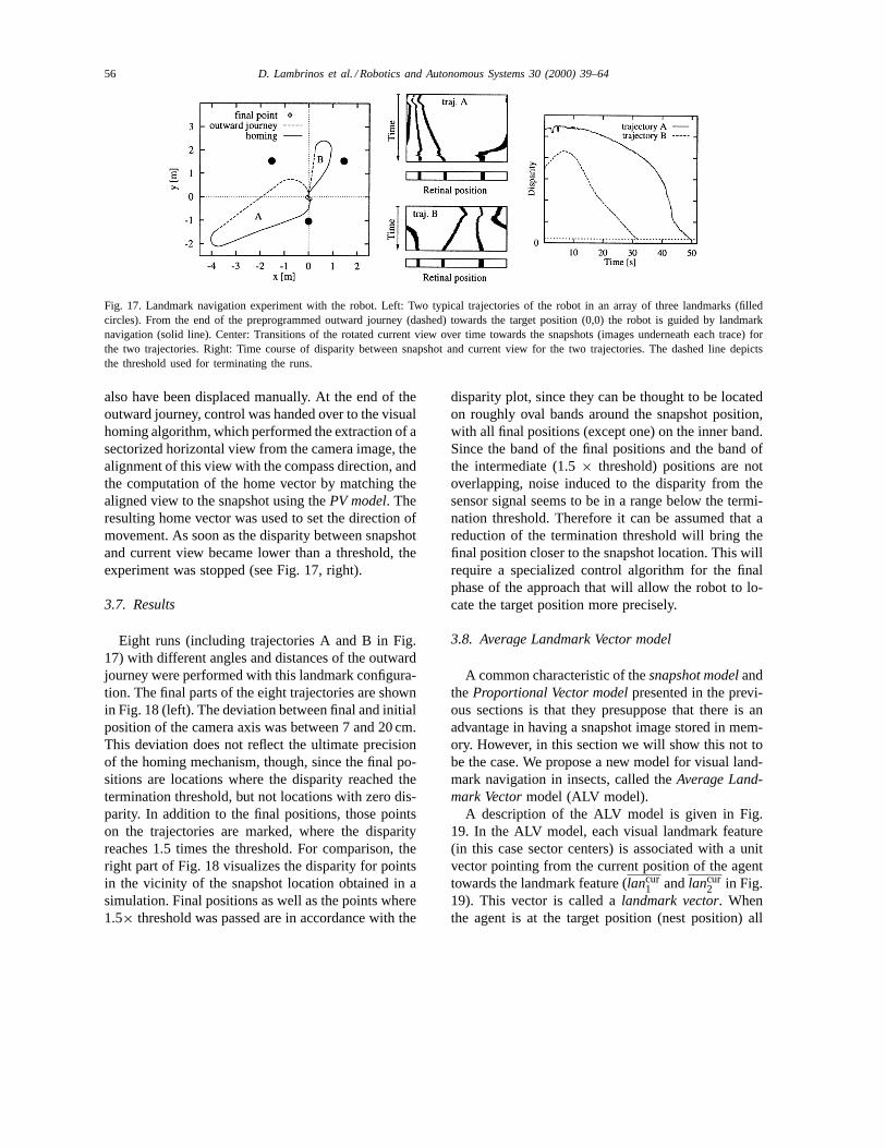
Fig. 17. Landmark navigation experiment with the robot. Left: Two typical trajectories of the robot in an array of three landmarks (filledcircles). From the end of the preprogrammed outward journey (dashed) towards the target position (0,0) the robot is guided by landmarknavigation (solid line). Center: Transitions of the rotated current view over time towards the snapshots (images underneath each trace) forthe two trajectories. Right: Time course of disparity between snapshot and current view for the two trajectories. The dashed line depictsthe threshold used for terminating the runs.
also have been displaced manually. At the end of theoutward journey, control was handed over to the visualhoming algorithm, which performed the extraction of asectorized horizontal view from the camera image, thealignment of this view with the compass direction, andthe computation of the home vector by matching thealigned view to the snapshot using thePV model. Theresulting home vector was used to set the direction ofmovement. As soon as the disparity between snapshotand current view became lower than a threshold, theexperiment was stopped (see Fig. 17, right).
3.7. Results
Eight runs (including trajectories A and B in Fig.17) with different angles and distances of the outwardjourney were performed with this landmark configura-tion. The final parts of the eight trajectories are shownin Fig. 18 (left). The deviation between final and initialposition of the camera axis was between 7 and 20 cm.This deviation does not reflect the ultimate precisionof the homing mechanism, though, since the final po-sitions are locations where the disparity reached thetermination threshold, but not locations with zero dis-parity. In addition to the final positions, those pointson the trajectories are marked, where the disparityreaches 1.5 times the threshold. For comparison, theright part of Fig. 18 visualizes the disparity for pointsin the vicinity of the snapshot location obtained in asimulation. Final positions as well as the points where1.5× threshold was passed are in accordance with the
disparity plot, since they can be thought to be locatedon roughly oval bands around the snapshot position,with all final positions (except one) on the inner band.Since the band of the final positions and the band ofthe intermediate (1.5× threshold) positions are notoverlapping, noise induced to the disparity from thesensor signal seems to be in a range below the termi-nation threshold. Therefore it can be assumed that areduction of the termination threshold will bring thefinal position closer to the snapshot location. This willrequire a specialized control algorithm for the finalphase of the approach that will allow the robot to lo-cate the target position more precisely.
3.8. Average Landmark Vector model
A common characteristic of thesnapshot modelandtheProportional Vector modelpresented in the previ-ous sections is that they presuppose that there is anadvantage in having a snapshot image stored in mem-ory. However, in this section we will show this not tobe the case. We propose a new model for visual land-mark navigation in insects, called theAverage Land-mark Vectormodel (ALV model).
A description of the ALV model is given in Fig.19. In the ALV model, each visual landmark feature(in this case sector centers) is associated with a unitvector pointing from the current position of the agenttowards the landmark feature (lancur
1 andlancur2 in Fig.
19). This vector is called alandmark vector. Whenthe agent is at the target position (nest position) all
D. Lambrinos et al. / Robotics and Autonomous Systems 30 (2000) 39–64 57
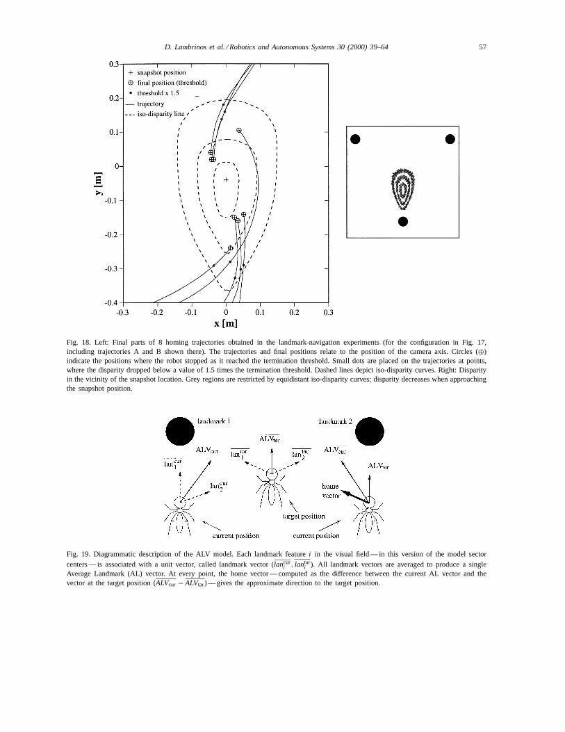
Fig. 18. Left: Final parts of 8 homing trajectories obtained in the landmark-navigation experiments (for the configuration in Fig. 17,including trajectories A and B shown there). The trajectories and final positions relate to the position of the camera axis. Circles (⊕)indicate the positions where the robot stopped as it reached the termination threshold. Small dots are placed on the trajectories at points,where the disparity dropped below a value of 1.5 times the termination threshold. Dashed lines depict iso-disparity curves. Right: Disparityin the vicinity of the snapshot location. Grey regions are restricted by equidistant iso-disparity curves; disparity decreases when approachingthe snapshot position.
Fig. 19. Diagrammatic description of the ALV model. Each landmark featurei in the visual field — in this version of the model sector
centers — is associated with a unit vector, called landmark vector (lancuri , lantar
i ). All landmark vectors are averaged to produce a singleAverage Landmark (AL) vector. At every point, the home vector — computed as the difference between the current AL vector and thevector at the target position (ALVcur − ALVtar) — gives the approximate direction to the target position.
58 D. Lambrinos et al. / Robotics and Autonomous Systems 30 (2000) 39–64
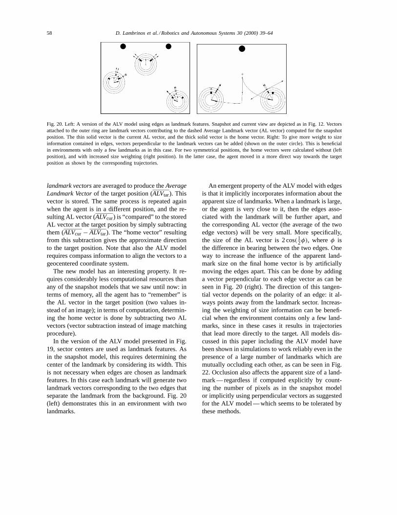
Fig. 20. Left: A version of the ALV model using edges as landmark features. Snapshot and current view are depicted as in Fig. 12. Vectorsattached to the outer ring are landmark vectors contributing to the dashed Average Landmark vector (AL vector) computed for the snapshotposition. The thin solid vector is the current AL vector, and the thick solid vector is the home vector. Right: To give more weight to sizeinformation contained in edges, vectors perpendicular to the landmark vectors can be added (shown on the outer circle). This is beneficialin environments with only a few landmarks as in this case. For two symmetrical positions, the home vectors were calculated without (leftposition), and with increased size weighting (right position). In the latter case, the agent moved in a more direct way towards the targetposition as shown by the corresponding trajectories.
landmark vectorsare averaged to produce theAverageLandmark Vectorof the target position (ALVtar). Thisvector is stored. The same process is repeated againwhen the agent is in a different position, and the re-sulting AL vector (ALVcur) is “compared” to the storedAL vector at the target position by simply subtractingthem (ALVcur − ALVtar). The “home vector” resultingfrom this subtraction gives the approximate directionto the target position. Note that also the ALV modelrequires compass information to align the vectors to ageocentered coordinate system.
The new model has an interesting property. It re-quires considerably less computational resources thanany of the snapshot models that we saw until now: interms of memory, all the agent has to “remember” isthe AL vector in the target position (two values in-stead of an image); in terms of computation, determin-ing the home vector is done by subtracting two ALvectors (vector subtraction instead of image matchingprocedure).
In the version of the ALV model presented in Fig.19, sector centers are used as landmark features. Asin the snapshot model, this requires determining thecenter of the landmark by considering its width. Thisis not necessary when edges are chosen as landmarkfeatures. In this case each landmark will generate twolandmark vectors corresponding to the two edges thatseparate the landmark from the background. Fig. 20(left) demonstrates this in an environment with twolandmarks.
An emergent property of the ALV model with edgesis that it implicitly incorporates information about theapparent size of landmarks. When a landmark is large,or the agent is very close to it, then the edges asso-ciated with the landmark will be further apart, andthe corresponding AL vector (the average of the twoedge vectors) will be very small. More specifically,the size of the AL vector is 2 cos(1
2φ), whereφ isthe difference in bearing between the two edges. Oneway to increase the influence of the apparent land-mark size on the final home vector is by artificiallymoving the edges apart. This can be done by addinga vector perpendicular to each edge vector as can beseen in Fig. 20 (right). The direction of this tangen-tial vector depends on the polarity of an edge: it al-ways points away from the landmark sector. Increas-ing the weighting of size information can be benefi-cial when the environment contains only a few land-marks, since in these cases it results in trajectoriesthat lead more directly to the target. All models dis-cussed in this paper including the ALV model havebeen shown in simulations to work reliably even in thepresence of a large number of landmarks which aremutually occluding each other, as can be seen in Fig.22. Occlusion also affects the apparent size of a land-mark — regardless if computed explicitly by count-ing the number of pixels as in the snapshot modelor implicitly using perpendicular vectors as suggestedfor the ALV model — which seems to be tolerated bythese methods.
D. Lambrinos et al. / Robotics and Autonomous Systems 30 (2000) 39–64 59
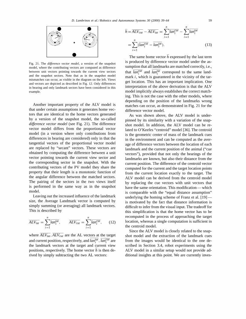
Fig. 21. Thedifference vector model, a version of the snapshotmodel, where the contributing vectors are computed as differencebetween unit vectors pointing towards the current view sectorsand the snapshot sectors. Note that as in the snapshot modelmismatches can occur, as visible in the diagram on the left. Viewsand vectors are depicted as described in Fig. 12. Only differencesin bearing and only landmark sectors have been considered in thisexample.
Another important property of the ALV model isthat under certain assumptions it generates home vec-tors that are identical to the home vectors generatedby a version of the snapshot model, the so-calleddifference vector model(see Fig. 21). The differencevector model differs from the proportional vectormodel (in a version where only contributions fromdifferences in bearing are considered) only in that thetangential vectors of the proportional vector modelare replaced by “secant” vectors. These vectors areobtained by computing the difference between a unitvector pointing towards the current view sector andthe corresponding sector in the snapshot. With thecontributing vectors of the PV model they share theproperty that their length is a monotonic function ofthe angular difference between the matched sectors.The pairing of the sectors in the two views itselfis performed in the same way as in the snapshotmodel.
Leaving out the increased influence of the landmarksize, the Average Landmark vector is computed bysimply summing (or averaging) all landmark vectors.This is described by
ALVtar =n∑
i=1
lantari , ALVcur =
n∑i=1
lancuri , (12)
whereALVtar, ALVcur are the AL vectors at the targetand current position, respectively, andlantar
i , lancuri are
the landmark vectors at the target and current viewpositions, respectively. The home vectorh is then de-rived by simply subtracting the two AL vectors:
h= ALVcur − ALVtar =n∑
i=1
lancuri −
n∑i=1
lantari
=n∑
i=1
(lancuri − lantar
i ). (13)
The same home vectorh expressed by the last termis produced by difference vector model under the as-sumption that all landmarks are matched correctly, i.e.,that lancur
i and lantari correspond to the same land-
mark i, which is guaranteed in the vicinity of the tar-get location. This has an important implication. Oneinterpretation of the above derivation is that the ALVmodel implicitly always establishes the correct match-ing. This is not the case with the other models, wheredepending on the position of the landmarks wrongmatches can occur, as demonstrated in Fig. 21 for thedifference vector model.
As was shown above, the ALV model is under-pinned by its similarity with a variation of the snap-shot model. In addition, the ALV model can be re-lated to O’Keefes “centroid” model [36]. The centroidis the geometric center of mass of the landmark cuesin the environment and can be computed as the aver-age of difference vectors between the location of eachlandmark and the current position of the animal (“cuevectors”), provided that not only the bearings of thelandmarks are known, but also their distance from thecurrent position. The difference of the centroid vectorcomputed for the current and the target location pointsfrom the current location exactly to the target. TheALV model can be derived from the centroid modelby replacing the cue vectors with unit vectors thathave the same orientation. This modification — whichis comparable with the “equal distance assumption”underlying the homing scheme of Franz et al. [19] —is motivated by the fact that distance information isdifficult to infer from the visual input. The tradeoff forthis simplification is that the home vector has to berecomputed in the process of approaching the targetlocation, whereas a single computation is sufficient inthe centroid model.
Since the ALV model is closely related to the snap-shot model and the extraction of the landmark cuesfrom the images would be identical to the one de-scribed in Section 3.4, robot experiments using theALV model in a similar setup would not provide ad-ditional insights at this point. We are currently inves-
60 D. Lambrinos et al. / Robotics and Autonomous Systems 30 (2000) 39–64
tigating the application of the ALV model to indoornavigation in an office environment.
3.9. Discussion
Panoramic vision systems of the type that is usedon theSahabot 2— a camera with vertical optical axisfacing a convex mirror — are a relatively simple tech-nical solution to obtain a 360◦ view, compared to theuse of multiple or rotating cameras. In the presentstudy, this vision system emulates the full or almostfull panoramic vision of insects [46,48], at least nearthe horizonal plane. Of course, the rectangular CCDsensor does not reproduce the distribution of omma-tidia across the insect eye. In the eyes ofCataglyphisbicolor, maximum resolution (3◦) is reached in thoseparts that look at the horizon, whereas the resolution issmaller in the upper and lower half of the eye (7◦) [46].In the technical vision system, resolution increaseswith increasing elevation of the pixel, but since onlythe horizonal portion is extracted from the polar view(see Fig. 15), this difference can be neglected. In theant’s eyes, the 3◦ resolution is approximately constantalong the horizon, which is also the case for the tech-nical counterpart with its 2◦ resolution. The resolu-tion is limiting for the application range of the visualhoming mechanism: as visible in Fig. 17, in a distanceof approximately 4 m the landmarks occasionally dis-appear from the sectorized image.
It would have been interesting to use in our robot ex-periments those landmarks that are relevant to the antsin their natural habitat. However, whereas the ant’seyes are about 0.5 cm above ground, the mirror of therobot’s visual system is at 27 cm height. Objects likesmall shrubs or stones that stick above the horizon ofthe ants and are therefore visible as a skyline againstthe bright sky as background may be far below thehorizon for the robot. From its higher perspective, thefrequent shrubs in the vicinity of the test field form asingle band around the horizon which can not be sep-arated into distinct landmarks. Therefore in the exper-iments black cylinders (as visible in Fig. 16) — of thesame type also used in the ant experiments — servedas landmarks.
In this environment and with the artificial land-marks, simple image processing steps are sufficient tolink the camera image with the representation requiredfor thesnapshot model. For natural landmarks and en-
vironments without the advantage of a free horizon,more elaborate image processing routines will be nec-essary. The application of a functionally similar hom-ing method to indoor navigation is currently under in-vestigation.
The snapshot modelwas developed in order to re-produce the search behavior of bees [6]. Experimentshave shown that the basic assumption — a snapshotimage or information derived from this image is storedin the target position — also holds for ants [52,54].However, details about the form of this snapshot (im-age, vector) and the specific method ants use to de-rive a home vector by matching snapshot and cur-rent view are not known so far. A systematic inves-tigation would be necessary to find out if the match-ing procedure suggested in [6] or variations of it likethe proportional vector model(Section 3.3), thedif-ference vector model(Section 3.8), or theALV model(Section 3.8) correctly predict the search behavior ofants in modified landmark setups. For this purpose,also the influence of the apparent height of the land-marks has to be considered, which has been neglectedin our computer simulations and robot experiments upto now.
While it is difficult to compare the precision of thepath-integration system of robot and ants (see Section2.8), it is legitimate to compare the precision of thevisual homing methods, since the visual processing isnot affected by differences in size or propulsion. Theprecision achieved in the robot experiments — with thegiven threshold, the final distance to the snapshot loca-tion ranged between 7 and 20 cm (see Section 3.7) —is in a range where an ant should be able to see orsmell the nest entrance. Demonstrating that this pre-cision can be achieved in real-world experiments pro-vides strong support for the snapshot thesis and thespecific matching procedure.
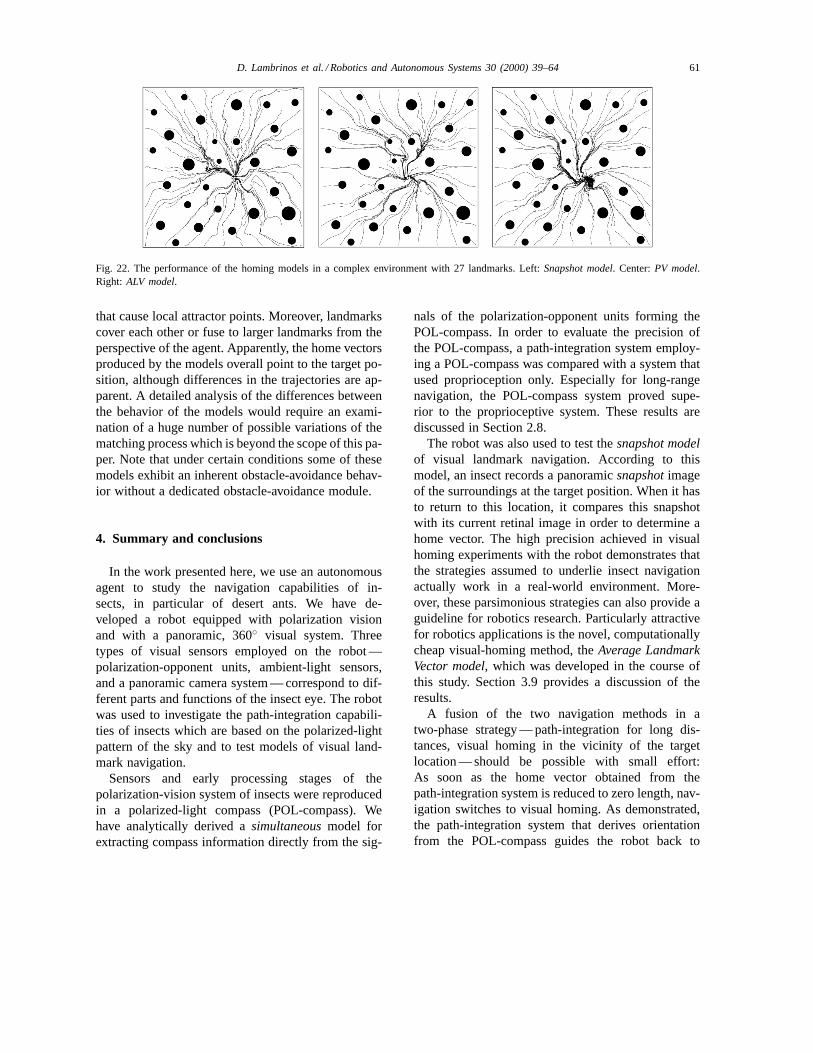
The setups used in the robot experiments consistedof 2–4 landmarks. Computer simulations revealed thatdespite the parsimony of all models (and especially oftheALV model) even complex landmark situations canbe mastered. Fig. 22 shows how three of the models(original snapshot model, PV model, andALV model)perform in a complex environment with 27 landmarksof different sizes. All models perform surprisinglywell, generating trajectories that end at the target po-sition. The expectation was that because of the largenumber of landmarks many false matches would occur
D. Lambrinos et al. / Robotics and Autonomous Systems 30 (2000) 39–64 61
Fig. 22. The performance of the homing models in a complex environment with 27 landmarks. Left:Snapshot model. Center:PV model.Right: ALV model.
that cause local attractor points. Moreover, landmarkscover each other or fuse to larger landmarks from theperspective of the agent. Apparently, the home vectorsproduced by the models overall point to the target po-sition, although differences in the trajectories are ap-parent. A detailed analysis of the differences betweenthe behavior of the models would require an exami-nation of a huge number of possible variations of thematching process which is beyond the scope of this pa-per. Note that under certain conditions some of thesemodels exhibit an inherent obstacle-avoidance behav-ior without a dedicated obstacle-avoidance module.
4. Summary and conclusions
In the work presented here, we use an autonomousagent to study the navigation capabilities of in-sects, in particular of desert ants. We have de-veloped a robot equipped with polarization visionand with a panoramic, 360◦ visual system. Threetypes of visual sensors employed on the robot —polarization-opponent units, ambient-light sensors,and a panoramic camera system — correspond to dif-ferent parts and functions of the insect eye. The robotwas used to investigate the path-integration capabili-ties of insects which are based on the polarized-lightpattern of the sky and to test models of visual land-mark navigation.
Sensors and early processing stages of thepolarization-vision system of insects were reproducedin a polarized-light compass (POL-compass). Wehave analytically derived asimultaneousmodel forextracting compass information directly from the sig-
nals of the polarization-opponent units forming thePOL-compass. In order to evaluate the precision ofthe POL-compass, a path-integration system employ-ing a POL-compass was compared with a system thatused proprioception only. Especially for long-rangenavigation, the POL-compass system proved supe-rior to the proprioceptive system. These results arediscussed in Section 2.8.
The robot was also used to test thesnapshot modelof visual landmark navigation. According to thismodel, an insect records a panoramicsnapshotimageof the surroundings at the target position. When it hasto return to this location, it compares this snapshotwith its current retinal image in order to determine ahome vector. The high precision achieved in visualhoming experiments with the robot demonstrates thatthe strategies assumed to underlie insect navigationactually work in a real-world environment. More-over, these parsimonious strategies can also provide aguideline for robotics research. Particularly attractivefor robotics applications is the novel, computationallycheap visual-homing method, theAverage LandmarkVector model, which was developed in the course ofthis study. Section 3.9 provides a discussion of theresults.
A fusion of the two navigation methods in atwo-phase strategy — path-integration for long dis-tances, visual homing in the vicinity of the targetlocation — should be possible with small effort:As soon as the home vector obtained from thepath-integration system is reduced to zero length, nav-igation switches to visual homing. As demonstrated,the path-integration system that derives orientationfrom the POL-compass guides the robot back to
62 D. Lambrinos et al. / Robotics and Autonomous Systems 30 (2000) 39–64
the vicinity of the starting location with a precisionof better than 1 m even after excursions of severalhundred meters length. Visual piloting, on the otherhand, has been shown to work in a range of up to 4 mwith the given landmark setup, camera resolution,and image processing steps. The overlap of the twoworking ranges is indicating that a two-phase strategycan be successful. Recently, new experimental resultsconcerning the interplay of path integration and land-mark navigation have been presented [11]. Moreover,extensions of the visual homing method may increaseits working range. The use of multiple snapshots wassuggested in [7] and currently received support fromant experiments [24].
This case study illustrates the power of bioroboticsthat arises from the close relationship between engi-neering and biology: On the one hand, insights for in-novative engineering designs can be found by analyz-ing the mechanisms employed by biological agents.On the other hand, biological hypotheses can be con-firmed using real-world artifacts rather than simula-tions only, and new biological hypotheses and ideasfor new animal experiments can be generated. Futurework will concentrate on adapting the parsimoniousstrategies of insects for landmark navigation in indoorenvironments.
Acknowledgements
This work is supported by the Swiss NationalScience Foundation (grants 20-47257.96 and 2000-053915.98 to R. Pfeifer and 31-43317.95 to R.Wehner), the Swiss Federal Office for Educationand Science (VIRGO TMR network), and the Hu-man Frontier Science Program. TheSahabot 2wasconstructed in cooperation with Rosys AG, Hom-brechtikon. Financial support by Rosys AG is kindlyacknowledged. The authors thank Christian Gfeller(Rosys) for the fruitful cooperation. Many thanksto Marinus Maris and Hiroshi Kobayashi for theircontributions in the construction of the robot.
References
[1] B. Barshan, H.F. Durrant-Whyte, Orientation estimate formobile robots using gyroscopic information, in: Proceedingsof the International Conference on Intelligent Robots andSystems (IROS 94), 1994, pp. 1867–1874.
[2] B. Barshan, H.F. Durrant-Whyte, Inertial navigation systemsfor mobile robots, Transactions on Robotics and Automation11 (1995) 328–342.
[3] S.L. Bartlett, A. Hampapur, M.J. Huber, D. Kortenkamp, S.Moezzi, Vision for mobile robots, in: J. Sanz (Ed.), Advancesin Image Processing and Machine Vision, Springer, Berlin,1995, pp. 1–117.
[4] G.D. Bernard, R. Wehner, Functional similarities betweenpolarization vision and color vision, Vision Research 17(1977) 1019–1028.
[5] J. Borenstein, H.R. Everett, L. Feng, “Where am I?” Sensorsand methods for mobile robot positioning, Technical Report,University of Michigan, 1996.
[6] B.A. Cartwright, T.S. Collett, Landmark learning in bees,Journal of Comparative Physiology 151 (1983) 521–543.
[7] B.A. Cartwright, T.S. Collett, Landmark maps for honeybees,Biological Cybernetics 57 (1987) 85–93.
[8] R. Cassinis, D. Grana, A. Rizzi, Using colour information inan omnidirectional perception system for autonomous robotlocalization, in: Proceedings of the First Euromicro Workshopon Advanced Mobile Robots (EUROBOT ’96), Los Alamitos,CA, 9–11 October 1996, IEEE Computer Society Press, SilverSpring, MD, 1996.
[9] J.S. Chahl, M.V. Srinivasan, Visual computation ofegomotion using an image interpolation technique, BiologicalCybernetics 74 (1996) 405–411.
[10] J.S. Chahl, M.V. Srinivasan, Reflective surfaces for panoramicimaging, Applied Optics 36 (31) (1997) 8275–8285.
[11] M. Collett, T.S. Collett, S. Bisch, R. Wehner, Local and globalvectors in desert ant navigation, Nature 394 (1998) 269–272.
[12] T.S. Collett, J. Baron, Biological compasses and thecoordinate frame of landmark memories in honeybees, Nature368 (1994) 137–140.
[13] T. Consi, J. Atema, J. Cho, C. Chryssostomidis, AUVguidance with chemical signals, in: Proceedings of the IEEESymposium on Autonomous Underwater Vehicle Technology,Cambridge, MA, 19–20 July 1994, pp. 3–9.
[14] H. Cruse, Ch. Bartling, G. Cymbalyuk, J. Dean, M. Dreifert,A modular artificial neural net for controlling a six-leggedwalking system, Biological Cybernetics 72 (1995) 421–430.
[15] H. Cruse, Ch. Bartling, J. Dean, T. Kindermann, J. Schmitz,M. Schumm, H. Wagner, Coordination in a six-leggedwalking system. Simple solutions to complex problems byexploitation of physical properties, in: Proceedings of theFourth International Conference on Simulation of AdaptiveBehavior, From Animals to Animats (SAB96), Cape Cod,MA, 1996, pp. 84–93.
[16] F.C. Dyer, J.A. Dickinson, Development of sun compensationby honey bees: How partially experienced bees estimatethe sun’s course, Proceedings of the National Academy ofScience, USA 91 (1994) 4471–4474.
[17] N. Franceschini, J.M. Pichon, C. Blanes, From insect vision torobot vision, Philosophical Transactions of the Royal Societyof London 337 (1992) 283–294.
[18] M.O. Franz, B. Schölkopf, H.A. Mallot, H.H. Bülthoff,Learning view graphs for robot navigation, AutonomousRobots 5 (1998) 111–125.
D. Lambrinos et al. / Robotics and Autonomous Systems 30 (2000) 39–64 63
[19] M.O. Franz, B. Schölkopf, H.A. Mallot, H.H. Bülthoff, Wheredid I take that snapshot? Scene-based homing by imagematching, Biological Cybernetics 79 (1998) 191–202.
[20] P. Gaussier, C. Joulain, S. Zrehen, J.P. Banquet, A. Revel,Visual navigation in an open environment without map, in:Proceedings of the IEEE/RSJ International Conference onIntelligent Robots and Systems (IROS-97) 1997, pp. 545–550.
[21] F. Grasso, T. Consi, D. Mountain, J. Atema, Locatingodor sources in turbulence with a lobster inspired robot,in: Proceedings of the Fourth International Conference onSimulation of Adaptive Behavior, From Animals to Animats(SAB96), Cape Cod, MA, 1996, pp. 104–112.
[22] G. Hartmann, R. Wehner, The ant’s path integration system:A neural architecture, Biological Cybernetics 73 (6) (1995)483–493.
[23] J. Hong, X. Tan, B. Pinette, R. Weiss, E.M. Riseman,Image-based homing, IEEE Control Systems (February 1992)104–112.
[24] S.P.D. Judd, T.S. Collett, Multiple stored views and landmarkguidance in ants, Nature 392 (1998) 710–714.
[25] D. Kortenkamp, Cognitive maps for mobile robots: Arepresentation for mapping and navigation, PhD thesis, TheUniversity of Michigan, 1993.
[26] B. J. Kuipers, Y. T. Byun, A robust, qualitative method forrobot spatial learning, in: Proceedings of the 7th NationalConference on Artificial Intelligence (AAAI-88), St. Paul,MN, Morgan Kaufmann, Los Altos, CA, 1988, pp. 774–779.
[27] T. Labhart, Polarization-opponent interneurons in the insectvisual system, Nature 331 (1988) 435–437.
[28] T. Labhart, Unpublished results, 1998.[29] D. Lambrinos, M. Maris, H. Kobayashi, T. Labhart, R. Pfeifer,
R. Wehner, An autonomous agent navigating with a polarizedlight compass, Adaptive Behavior 6 (1) (1997) 131–161.
[30] M. Lindauer, Angeborene und erlernte Komponenten in derSonnenorientierung der Bienen, Zeitschrift für vergleichendePhysiologie 42 (1959) 43–62.
[31] H. Lund, B. Webb, J. Hallam, A robot attracted to the cricketspecies gryllus bimaculatus, in: Proceedings of the FourthEuropean Conference on Artificial Life, 1997, pp. 131–140.
[32] L. Matthies, E. Gat, R. Harrison, Mars microrover navigation:Performance evaluation and enhancement, Technical Report95-0096, Jet Propulsion Laboratory, NASA, Pasadena, CA,1995.
[33] R. Möller, M. Maris, D. Lambrinos, A neural modelof landmark navigation in insects, Neurocomputing 26–27(1999) 801–808.
[34] M. Müller, R. Wehner, Path integration in desert ants,Cataglyphis fortis, Proceedings of the National Academy ofScience Neurobiology 85 (1988) 5287–5290.
[35] R.C. Nelson, Visual homing using an associative memory, in:Proceedings of the Image Understanding Workshop, MorganKaufmann, Palo Alto, CA, May 1989, pp. 245–262.
[36] J. O’Keefe, The hippocampal cognitive map and navigationalstrategies, in: J. Paillard (Ed.), Brain and Space, OxfordUniversity Press, Oxford, 1991, Chapter 16, pp. 273–295.
[37] R. Pfeifer, Building “fungus eaters”: Design principlesof autonomous agents, in: Proceedings of the Fourth
International Conference on Simulation of Adaptive Behavior,From Animals to Animats (SAB96), Cape Cod, MA, 1996,pp. 3–12.
[38] M.V. Srinivasan, An image-interpolation technique for thecomputation of optic flow and egomotion, BiologicalCybernetics 71 (1994) 401–416.
[39] M.V. Srinivasan, J.S. Chahl, S.W. Zhang, Robot navigation byvisual dead-reckoning: Inspiration from insects, InternationalJournal of Pattern Recognition and Artificial Intelligence11 (1) (1997) 35–47.
[40] H. Vitzthum, Der Zentralkomplex der HeuschreckeSchistocerca gregaria: Ein mögliches Zentrum desPolarisationssehsystems, PhD thesis, Universität Regensburg,1997.
[41] B. Webb, Robotic experiments in cricket phonotaxis, in:Proceedings of the Third International Conference onSimulation of Adaptive Behavior, From Animals to Animats3 (SAB94), MIT Press, Cambridge, MA, 1994, pp. 45–54.
[42] B. Webb, Biological orientation systems for mobile robots,in: Proceedings of the International Conference on RecentAdvances in Mechatronics, 1995.
[43] B. Webb, Using robots to model animals: A cricket test,Robotics and Autonomous Systems 16 (2–4) (1995) 117–134.
[44] B. Webb, A cricket robot, Scientific American 275 (6) (1996)94–99.
[45] B. Webb, J. Hallam, How to attract females: Further roboticexperiments in cricket phonotaxis, in: Proceedings of theFourth International Conference on Simulation of AdaptiveBehavior, From Animals to Animats 4 (SAB96), Cape Cod,MA, MIT Press, Cambridge, MA, 1996, pp. 75–83.
[46] R. Wehner, Himmelsnavigation bei Insekten. Neurophysio-logie und Verhalten, Neujahrbl. Naturforsch. Ges. Zürich 184(1982) 1–132.
[47] R. Wehner, Spatial organization of foraging behavior inindividually searching desert ants,Cataglyphis(Sahara desert)and Ocymyrmex (Namib desert), in: J.M. Pasteels, J.L.Deneubourg (Eds.), From Individual to Collective Behaviorin Social Insects, Birkhäuser, Basel, 1987, pp. 15–42.
[48] R. Wehner, Arthropods, in: F. Papi (Ed.), Animal Homing,Chapman and Hall Animal Behaviour Series, Chapman andHall, London, 1992, Chapter 3, pp. 45–127.
[49] R. Wehner, The polarization-vision project: Championingorganismic biology, in: K. Schildberger, N. Elsner (Eds.),Neural Basis of Behavioural Adaptations, Gustav FischerVerlag, Stuttgart, 1994, pp. 103–143.
[50] R. Wehner, The ant’s celestial compass system: Spectraland polarization channels, Orientation and Communication inArthropods, Birkhäuser, Basel, 1997, pp. 145–185.
[51] R. Wehner, B. Lanfranconi, What do the ants know about therotation of the sky?, Nature 293 (1981) 731–773.
[52] R. Wehner, B. Michel, P. Antonsen, Visual navigation ininsects: Coupling of egocentric and geocentric information,Journal of Experimental Biology 199 (1996) 129–140.
[53] R. Wehner, M. Müller, How do ants acquire their celestialephemeris function? Naturwissenschaften 331–333 (1993)4471–4474.
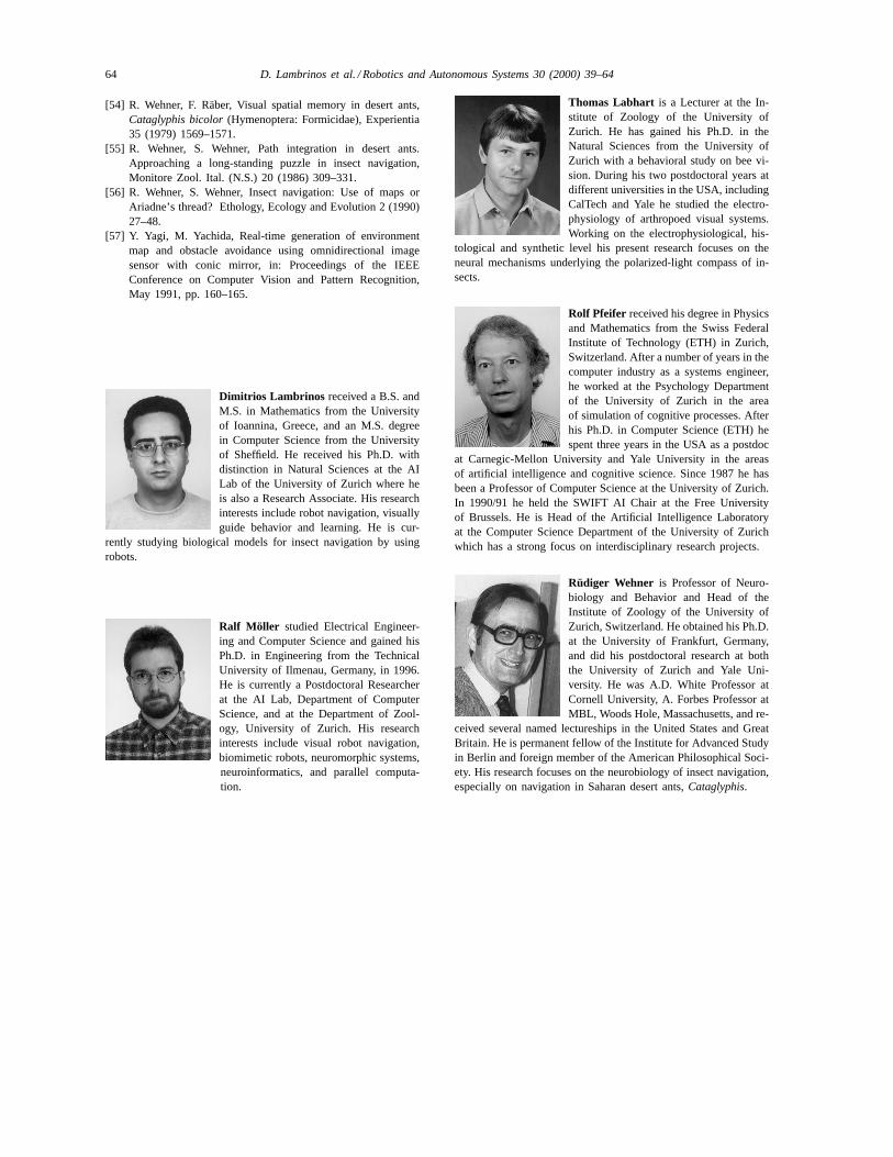
64 D. Lambrinos et al. / Robotics and Autonomous Systems 30 (2000) 39–64
[54] R. Wehner, F. Räber, Visual spatial memory in desert ants,Cataglyphis bicolor(Hymenoptera: Formicidae), Experientia35 (1979) 1569–1571.
[55] R. Wehner, S. Wehner, Path integration in desert ants.Approaching a long-standing puzzle in insect navigation,Monitore Zool. Ital. (N.S.) 20 (1986) 309–331.
[56] R. Wehner, S. Wehner, Insect navigation: Use of maps orAriadne’s thread? Ethology, Ecology and Evolution 2 (1990)27–48.
[57] Y. Yagi, M. Yachida, Real-time generation of environmentmap and obstacle avoidance using omnidirectional imagesensor with conic mirror, in: Proceedings of the IEEEConference on Computer Vision and Pattern Recognition,May 1991, pp. 160–165.
Dimitrios Lambrinos received a B.S. andM.S. in Mathematics from the Universityof Ioannina, Greece, and an M.S. degreein Computer Science from the Universityof Sheffield. He received his Ph.D. withdistinction in Natural Sciences at the AILab of the University of Zurich where heis also a Research Associate. His researchinterests include robot navigation, visuallyguide behavior and learning. He is cur-
rently studying biological models for insect navigation by usingrobots.
Ralf Möller studied Electrical Engineer-ing and Computer Science and gained hisPh.D. in Engineering from the TechnicalUniversity of Ilmenau, Germany, in 1996.He is currently a Postdoctoral Researcherat the AI Lab, Department of ComputerScience, and at the Department of Zool-ogy, University of Zurich. His researchinterests include visual robot navigation,biomimetic robots, neuromorphic systems,neuroinformatics, and parallel computa-tion.
Thomas Labhart is a Lecturer at the In-stitute of Zoology of the University ofZurich. He has gained his Ph.D. in theNatural Sciences from the University ofZurich with a behavioral study on bee vi-sion. During his two postdoctoral years atdifferent universities in the USA, includingCalTech and Yale he studied the electro-physiology of arthropoed visual systems.Working on the electrophysiological, his-
tological and synthetic level his present research focuses on theneural mechanisms underlying the polarized-light compass of in-sects.
Rolf Pfeifer received his degree in Physicsand Mathematics from the Swiss FederalInstitute of Technology (ETH) in Zurich,Switzerland. After a number of years in thecomputer industry as a systems engineer,he worked at the Psychology Departmentof the University of Zurich in the areaof simulation of cognitive processes. Afterhis Ph.D. in Computer Science (ETH) hespent three years in the USA as a postdoc
at Carnegic-Mellon University and Yale University in the areasof artificial intelligence and cognitive science. Since 1987 he hasbeen a Professor of Computer Science at the University of Zurich.In 1990/91 he held the SWIFT AI Chair at the Free Universityof Brussels. He is Head of the Artificial Intelligence Laboratoryat the Computer Science Department of the University of Zurichwhich has a strong focus on interdisciplinary research projects.
Rüdiger Wehner is Professor of Neuro-biology and Behavior and Head of theInstitute of Zoology of the University ofZurich, Switzerland. He obtained his Ph.D.at the University of Frankfurt, Germany,and did his postdoctoral research at boththe University of Zurich and Yale Uni-versity. He was A.D. White Professor atCornell University, A. Forbes Professor atMBL, Woods Hole, Massachusetts, and re-
ceived several named lectureships in the United States and GreatBritain. He is permanent fellow of the Institute for Advanced Studyin Berlin and foreign member of the American Philosophical Soci-ety. His research focuses on the neurobiology of insect navigation,especially on navigation in Saharan desert ants,Cataglyphis.