Embed Size (px)
Citation preview

Active Vision Laboratory
Robot Navigation
by
Active Stereo Vision
Joss Knight
D.Phil First Year Report
Report No. OUEL 2220/00
Robotics Research GroupDepartment of Engineering Science
University of OxfordParks Road
Oxford OX1 3PJUK
Tel: +44 865 273168Fax: +44 865 273908
Email: [email protected]
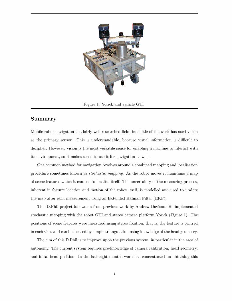
Figure 1: Yorick and vehicle GTI
Summary
Mobile robot navigation is a fairly well researched field, but little of the work has used vision
as the primary sensor. This is understandable, because visual information is difficult to
decipher. However, vision is the most versatile sense for enabling a machine to interact with
its environment, so it makes sense to use it for navigation as well.
One common method for navigation revolves around a combined mapping and localisation
procedure sometimes known as stochastic mapping. As the robot moves it maintains a map
of scene features which it can use to localise itself. The uncertainty of the measuring process,
inherent in feature location and motion of the robot itself, is modelled and used to update
the map after each measurement using an Extended Kalman Filter (EKF).
This D.Phil project follows on from previous work by Andrew Davison. He implemented
stochastic mapping with the robot GTI and stereo camera platform Yorick (Figure 1). The
positions of scene features were measured using stereo fixation, that is, the feature is centred
in each view and can be located by simple triangulation using knowledge of the head geometry.
The aim of this D.Phil is to improve upon the previous system, in particular in the area of
autonomy. The current system requires pre-knowledge of camera calibration, head geometry,
and inital head position. In the last eight months work has concentrated on obtaining this
i

information automatically. Reid and Beardsley [39] showed that it was possible to self-align
the camera using controlled motions of the head from a position of zero knowledge. This
report explains their theory and shows how it can be extended to situations where there is
some degeneracy in the scene, such as the case that scene structure lies in a single plane. It
also shows how calculation of the camera calibration and head geometry is inherent in the
self-alignment process.
The mathematical theory of self-alignment is sound, and this was born out by tests using
simulated data. So far, however, it has not been possible to show the alignment process work-
ing repeatedly with real scenes. The problem lies in the difficulty of obtaining enough robust
information to overcome problems of noise and mismatching of image features. Simulation
indicated that most of the problem lies in matching of feature points between stereo images
well enough to obtain good 3D scene structure, which was implemented using standard algo-
rithms, rather than devised specifically for this work. However, the results indicate that the
procedure can be made to work consistently, and are therefore generally encouraging.
Alignment of the main gaze axis, the pan, depends on whichever direction is chosen to
be ‘forwards’. It is useful to be able to find this direction from the image sequence as the
robot moves alone. Such a calculation can be done easily off-line using standard techniques,
but more useful, particularly for obstacle avoidance, is a real time method. Therefore it was
decided to implement the pan axis alignment as a real time algorithm using optical flow.
The procedure was again shown to work under simulation, but demonstrated considerable
sensitivity to noisy input data. This resulted in failure to work well with real image sequences.
In addition, the method suffers from the restriction imposed by optical flow of only small
motion between images. Some further investigation, possibly into real-time outlier rejection,
may show uses for the technique, otherwise it must be considered inviable.
Future work will concentrate on integrating self-initialisation with the navigation process,
on speeding up stochastic mapping, and on obstacle avoidance. It is hope that by the end
it will be possible to demonstrate the same fully autonomous real time system running with
two different robot / stereo head rigs.
ii

CONTENTS CONTENTS
Contents
1 Introduction 1
2 Literature Review 3
2.1 Computer vision . . . . . . . . . . . . . . . . . . . . . . . . . . . . . . . . . . 3
2.2 Structure from motion . . . . . . . . . . . . . . . . . . . . . . . . . . . . . . . 3
2.3 Self-calibration . . . . . . . . . . . . . . . . . . . . . . . . . . . . . . . . . . . 5
2.4 Active vision . . . . . . . . . . . . . . . . . . . . . . . . . . . . . . . . . . . . 5
2.5 Navigation . . . . . . . . . . . . . . . . . . . . . . . . . . . . . . . . . . . . . . 6
2.6 Starting point – Andrew Davison’s PhD thesis . . . . . . . . . . . . . . . . . 7
2.7 Conclusions . . . . . . . . . . . . . . . . . . . . . . . . . . . . . . . . . . . . . 11
3 Notation and Basics 12
3.1 Homogeneous coordinates . . . . . . . . . . . . . . . . . . . . . . . . . . . . . 12
3.2 Points, lines, planes, and duality . . . . . . . . . . . . . . . . . . . . . . . . . 13
3.3 Perspective projection and camera matrices . . . . . . . . . . . . . . . . . . . 13
3.4 3-space and non-metric structure . . . . . . . . . . . . . . . . . . . . . . . . . 16
3.5 Multiple view geometry . . . . . . . . . . . . . . . . . . . . . . . . . . . . . . 17
3.6 Algorithms . . . . . . . . . . . . . . . . . . . . . . . . . . . . . . . . . . . . . 19
3.6.1 Disparity matching . . . . . . . . . . . . . . . . . . . . . . . . . . . . . 19
3.6.2 The Direct Linear Transform . . . . . . . . . . . . . . . . . . . . . . . 20
3.6.3 RANSAC . . . . . . . . . . . . . . . . . . . . . . . . . . . . . . . . . . 20
3.6.4 Non-linear minimisation and bundle adjustment . . . . . . . . . . . . 21
3.6.5 Summary of two view matching procedure . . . . . . . . . . . . . . . . 22
4 Aligning the Elevation and Vergence 23
4.1 Theory . . . . . . . . . . . . . . . . . . . . . . . . . . . . . . . . . . . . . . . . 23
4.1.1 Groundwork . . . . . . . . . . . . . . . . . . . . . . . . . . . . . . . . 23
4.1.2 Identifying HPE . . . . . . . . . . . . . . . . . . . . . . . . . . . . . . . . 24
4.1.3 The Non-degenerate case . . . . . . . . . . . . . . . . . . . . . . . . . 24
iii
CONTENTS CONTENTS
4.1.4 The degenerate case . . . . . . . . . . . . . . . . . . . . . . . . . . . . 27
4.1.5 Fixating with zero knowledge . . . . . . . . . . . . . . . . . . . . . . . 29
4.2 Implementation . . . . . . . . . . . . . . . . . . . . . . . . . . . . . . . . . . . 30
4.2.1 Non-degenerate case . . . . . . . . . . . . . . . . . . . . . . . . . . . . 30
4.2.2 Degenerate case . . . . . . . . . . . . . . . . . . . . . . . . . . . . . . . 35
4.2.3 Fixation . . . . . . . . . . . . . . . . . . . . . . . . . . . . . . . . . . . 36
4.2.4 Self-calibration . . . . . . . . . . . . . . . . . . . . . . . . . . . . . . . 38
4.3 Experimentation . . . . . . . . . . . . . . . . . . . . . . . . . . . . . . . . . . 38
4.3.1 Non-degenerate case . . . . . . . . . . . . . . . . . . . . . . . . . . . . 38
4.3.2 Degenerate case . . . . . . . . . . . . . . . . . . . . . . . . . . . . . . . 42
4.3.3 Fixation . . . . . . . . . . . . . . . . . . . . . . . . . . . . . . . . . . . 44
4.3.4 Self-calibration . . . . . . . . . . . . . . . . . . . . . . . . . . . . . . . 44
5 Alignment with Forward Direction 45
5.1 Theory . . . . . . . . . . . . . . . . . . . . . . . . . . . . . . . . . . . . . . . . 45
5.1.1 Determining optical flow . . . . . . . . . . . . . . . . . . . . . . . . . . 46
5.2 Implementation . . . . . . . . . . . . . . . . . . . . . . . . . . . . . . . . . . . 47
5.3 Experimentation . . . . . . . . . . . . . . . . . . . . . . . . . . . . . . . . . . 48
5.3.1 Simulation . . . . . . . . . . . . . . . . . . . . . . . . . . . . . . . . . 48
5.3.2 Real data . . . . . . . . . . . . . . . . . . . . . . . . . . . . . . . . . . 49
5.3.3 Discussion . . . . . . . . . . . . . . . . . . . . . . . . . . . . . . . . . . 50
A Decomposing a 3D homography 51
B Summary of Notation and Equations 54
B.1 Notation . . . . . . . . . . . . . . . . . . . . . . . . . . . . . . . . . . . . . . . 54
B.2 Important Equations . . . . . . . . . . . . . . . . . . . . . . . . . . . . . . . . 55
iv
1 INTRODUCTION
1 Introduction
Of all the sensory tools employed by the Artificial Intelligence community, vision has under-
gone the greatest expansion in the last fifteen years. Mollified by the successes of chess-playing
computers and other seemingly intelligent systems, AI academics considered vision to be a
simple problem. One oft-repeated anecdote is that MIT professors gave the problem of vision
to a graduate student as a one-year Master’s degree. Just a few decades on, machine vision
occupies engineers in entire University departments, and is the sole business of a large number
of companies stretching across the globe.
The problem lay, as is often the case, in the AI community’s misunderstanding of the com-
plexity of the mammalian brain. Extracting useful information from images is not a single
problem but a large number of them, each individually vastly complicated: segmentation, ob-
ject recognition, 3D reconstruction, tracking, fixation, feedback. . . The advantage of investing
in vision research is that the information content of camera images is considerably greater
than that from any other sensor, if only it can be retrieved. A simple video sequence contains
scene shape, structure and colour, and the motion of the camera and objects in the scene, all
of which can be extracted by algorithms based in mathematical theory. In combination with
AI the sequence may provide the numbers and identities of objects (or people), predictions
of activities off-image or not contained within the sequence, or more esoterical qualities like
the expressions on people’s faces or identifying unusual or criminal activities.
Active vision is a field only studied in depth in the last few years. It allows for some form of
camera control, that is the motion or other properties (such as zoom, iris etc.) can be altered in
response to the scene. This simplifies many of the problems of computer vision because there
is prior knowledge about the kind of changes occurring from image to image. In addition
it is possible to choose objects in the scene for extra attention or tracking (with obvious
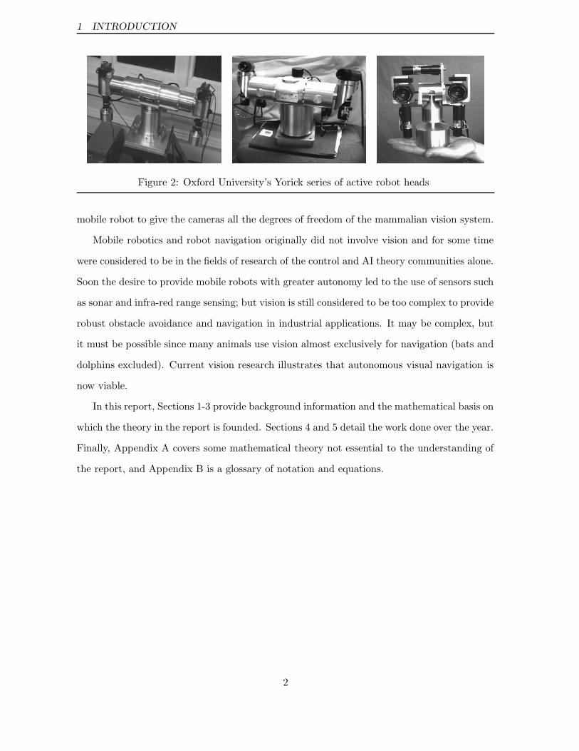
applications in security cameras, for instance). Recently the use of stereo pan-tilt heads has
become quite common (see Figure 2). Stereo cameras (useful because scene structure can be
extracted from a single pair of images) are generally mounted on individual vergence axes
with combined elevation and pan. It is a logical progression to mount the whole rig on a
1
1 INTRODUCTION
Figure 2: Oxford University’s Yorick series of active robot heads
mobile robot to give the cameras all the degrees of freedom of the mammalian vision system.
Mobile robotics and robot navigation originally did not involve vision and for some time
were considered to be in the fields of research of the control and AI theory communities alone.
Soon the desire to provide mobile robots with greater autonomy led to the use of sensors such
as sonar and infra-red range sensing; but vision is still considered to be too complex to provide
robust obstacle avoidance and navigation in industrial applications. It may be complex, but
it must be possible since many animals use vision almost exclusively for navigation (bats and
dolphins excluded). Current vision research illustrates that autonomous visual navigation is
now viable.
In this report, Sections 1-3 provide background information and the mathematical basis on
which the theory in the report is founded. Sections 4 and 5 detail the work done over the year.
Finally, Appendix A covers some mathematical theory not essential to the understanding of
the report, and Appendix B is a glossary of notation and equations.
2

2 LITERATURE REVIEW
2 Literature Review
2.1 Computer vision
Computer Vision can be defined along the lines of ‘using computers to discover from images
what is in a scene, and where it is’. The rules of perspective projection, a subset of projective
geometry which is the mathematical basis of image formation, have been around for centuries.
Many Renaissance artists used these rules to paint accurate representations of scenes — their
accuracy can be seen clearly from work by Antonio Criminisi in 3D reconstruction from single
views [8]. Certainly much of the geometrical and analytical tools which are now used in the
formation and interpretation of images have been around long enough for them to appear in
course notes and books [21, 34, 42, 48].
Attempting to interpret images is a younger research topic, with scientists studying the
psychology of vision (perception, optical illusions and so forth) and the neuroscience and
psychophysics (how the brain goes about image interpretation) only this century. Use of
computers in image analysis is perhaps nearly as old as computers but it wasn’t possible
to process anything but the simplest binary images until computers were powerful enough
in the late seventies. Only in the nineteen eighties and nineties has vision expanded into a
major research topic, as computing power accelerates as does the identification of profitable
applications.
Soon the main emphasis moved from image interpretation and object recognition to more
geometric interpretations of scenes. In particular, structure recovery became a heavily re-
searched topic. Structure from contours and structure from shading were attempts at struc-
ture recovery from single images that met with limited success. It was structure from motion
(and related structure from stereo) that was most successful.
2.2 Structure from motion
Early structure from motion concentrated on using calibrated cameras; that is the internal
parameters of the camera were assumed known and thus the 3D metric location of a point
matched in two views could be easily calculated. The remaining problems, therefore, were
only to match features between images in a sequence, and recover the motion of the camera
3

2 LITERATURE REVIEW 2.2 Structure from motion
(or of the scene). Perhaps the culmination of the latter research is the work of Tomasi and
Kanade [29, 44] in 1992 which introduced a factorisation method that is used in some form
in most structure recovery work today. The former problem, that of matching features, is
the bugbear of a huge variety of vision topics. One of the best algorithms for extracting
viewpoint-invariant features from images (usually termed ‘corners’ and ‘edges’) was by Harris
and Stephens [19], and it is Harris’ corner detector that has been used in this project. Match-
ing those features between views is still a major problem because most structure recovery
algorithms are extremely sensitive to mismatches, or outliers. Robust calculation of multiple
view relationships can still not be done in real time, but off-line robust feature matching algo-
rithms such as RANSAC (an iterative random sampling process) are now firmly established
and successful [45].
Camera calibration is a tiresome process and the 1990’s saw research into what structural
information could be obtained from uncalibrated views. Olivier Faugeras showed in 1992 that
matched points in two uncalibrated images could be used to obtain projective structure, a
representation that retains a few potentially exploitable properties. Hartley showed a similar
reconstruction for line correspondences [22].
Some research showed limited uses of projective structure in the areas of visual servoing
and robot navigation [1, 18]. However it was found much more could be done if the projective
structure was updated to affine, which retains useful properties such as length ratios and mid-
points. Beardsley et al. exploited this for robot navigation, mapping out free-space regions
in affine space and manoevring the camera down the centre-line [1, 2]. Various researchers
showed how it was possible to update projective to affine structure, and affine to metric, using
knowledge of certain constraints, or simply sufficient point matches and views, mostly using
stereo cameras [2, 3, 12, 49]. Horaud and Csurka showed updating to metric structure in a
single stage, ie. complete structure recovery from uncalibrated cameras, using at least two
motions of a stereo rig (two cameras fixed in relation to each other) [27]. However, structure
recovery from monocular image sequences is now quite advanced. Fitzgibbon and Zisserman
are able to reconstruct detailed models of the scene using simple video sequences, the last
remaining constraint being that the motion of the camera is sufficiently general [16].
4
2 LITERATURE REVIEW 2.3 Self-calibration
2.3 Self-calibration
Since structure can be recovered from images from uncalibrated cameras, that structure and
the corresponding image features can provide the camera internal parameters. Thus a camera
can be self-calibrated from sufficient images. The ease of self-calibration depends on scene
and camera motion. Initial research required general motion (rotation and translation) and
fixed camera parameters [15, 23, 25, 33]. Later extensions allowed some of the parameters to
vary between views [11, 26], the motion to be degenerate (rotation about the optical centre
only) [24], and the scene to be degenerate (planar) [47]. Other work includes Brooks et al.,
who developed a differential version of the fundamental matrix equation (see §3), and were
able to self-calibrate from optical flow alone [4, 5].
2.4 Active vision
Active vision allows for controlled camera motion, and this control can provide constraints
that make a great many problems in computer vision considerably more simple. Beardsley
and Zisserman used the constraint that their mobile robot moved in a single plane to calculate
affine structure from motion [3]. Horaud and Csurka, and Zisserman and Reid used controlled
motions of a stereo head for obtaining metric structure [27, 49]. And Reid and Beardsley used
known motions of a stereo head to calculate where the cameras should look for self-alignment
[39] (see §4).
Active vision also encompasses useful activities such as object tracking. The most robust
tracking uses a method known as transfer developed at Oxford by Reid, Murray and Fairley
[13, 14, 40]. But the use of active stereo camera platforms really comes into its own through
fixation. An object is fixated by stereo cameras if the object lies in a particular location in
each view (usually the principal point). An object can be located if fixated by triangulation
using the knowledge of the camera baseline (which can be learned if unknown). Many animals,
particularly those with forward-facing eyes, use fixation almost exclusively. In humans, for
instance, the eye tends to be in an endless loop of fixation followed by rapid motion (a saccade)
to fixate on a new object of interest. (In fact, we are not good at allowing the fixation point to
roam slowly over the scene, especially when moving about (ie. navigating)). Fixation is not
5
2 LITERATURE REVIEW 2.5 Navigation
only used to foveate the object of interest on the retina, but is important for structure recovery
and self-localisation. It seems sensible to see if fixation is suitable for robot navigation.
2.5 Navigation
Navigation was originally only studied in theory in the AI path-planning community. This
was because robots, certainly those in industry, will often follow specific paths such as lines
on the ground, or, for robot arms, there is pre-knowledge of the free space around the arm.
Thus the problem is one of planning the fastest path through the free space / network of lines
etc. Navigation is also of interest to the control community, for instance Pears and Bumby
investigated the best ways to follow lines given an offset as input [37]. As computer vision
became more sophisticated, visual feedback could be used in the control, such as in work done
at INRIA [7], but the premise is very much the same.
Autonomous navigation can be divided up into two elements – self-localisation, and ob-
stacle avoidance. Self-localisation is always necessary if the target cannot be guaranteed to
be in the field of view of the robot’s sensing device. Even if the robot has no specific target (it
has a wandering behaviour) it is of limited use unless it has some idea of its location relative
to its starting position.
Self-localisation using vision is not the hardest part of navigation because only a few visual
cues are required. Obstacle avoidance is a lot more difficult, however, because it is in general
not possible to guarantee that an obstacle will be detected (while it is just about possible with
sonar and other range-sensing devices). There has been some work on the control strategies
to be used where the required path is known and obstacle positions are known with some
level of uncertainty, such as Hu and Brady [28].
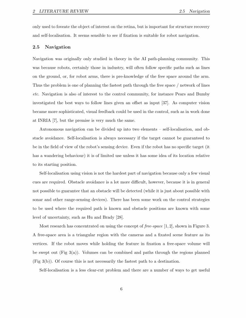
Most research has concentrated on using the concept of free-space [1, 2], shown in Figure 3.
A free-space area is a triangular region with the cameras and a fixated scene feature as its
vertices. If the robot moves while holding the feature in fixation a free-space volume will
be swept out (Fig 3(a)). Volumes can be combined and paths through the regions planned
(Fig 3(b)). Of course this is not necessarily the fastest path to a destination.
Self-localisation is a less clear-cut problem and there are a number of ways to get useful
6
2 LITERATURE REVIEW 2.6 Starting point – Andrew Davison’s PhD thesis
����������
�� ���������������������������������� ��
��������
(a) (b)
Figure 3: Use of free-space for obstacle avoidance. (a) Stereo cameras fixating a scene featurewhile moving to sweep out a free-space volume. (b) Combining free-space areas projected tothe ground plane to choose an obstacle-free path (blue line shows centre of free-space to oneobstacle) [3].
navigational information from images. Some use merely monocular cues such as optical flow,
which avoid the costly process of scene reconstruction [17, 41]. The work on which this thesis
is based relies on some limited reconstruction, but avoids the lengthy process of structure
from motion. Fixation and knowledge of the head geometry is used to calculate the 3-space
location of a limited number of features. The system, discussed briefly in the next section,
is layed out in full in Andrew Davison’s PhD thesis [9], and summarised in three papers by
Murray, Reid and Davison [10, 35, 36].
2.6 Starting point – Andrew Davison’s PhD thesis
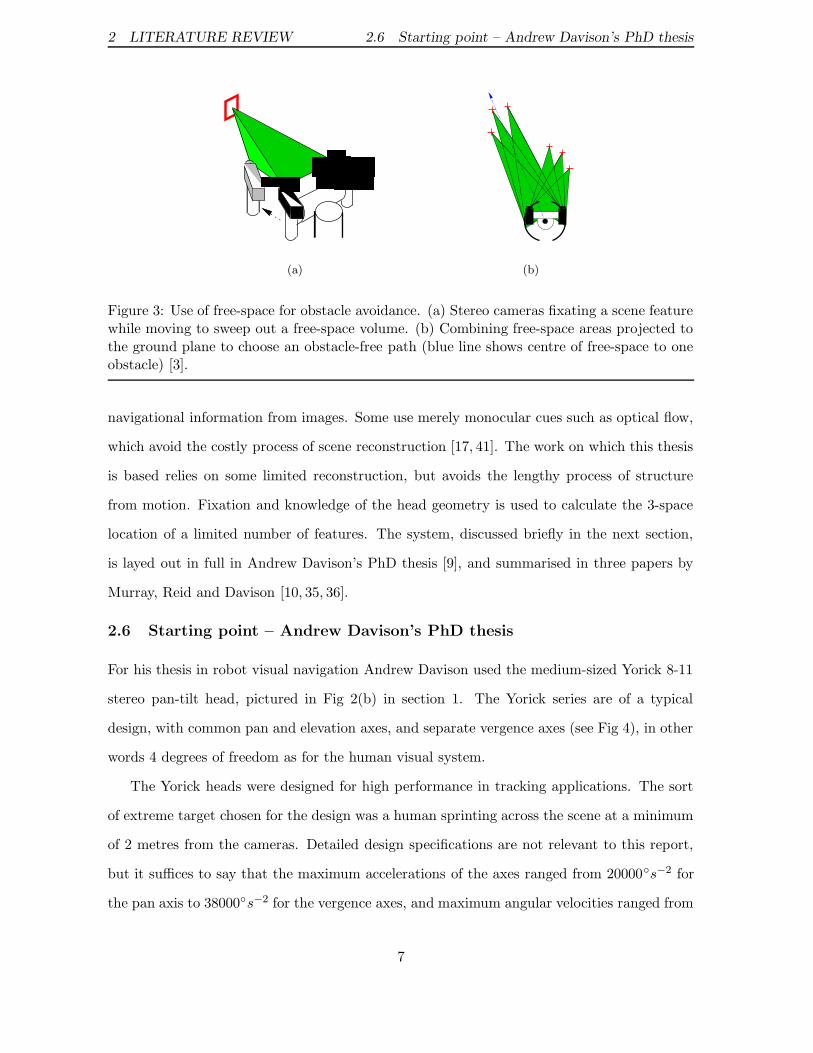
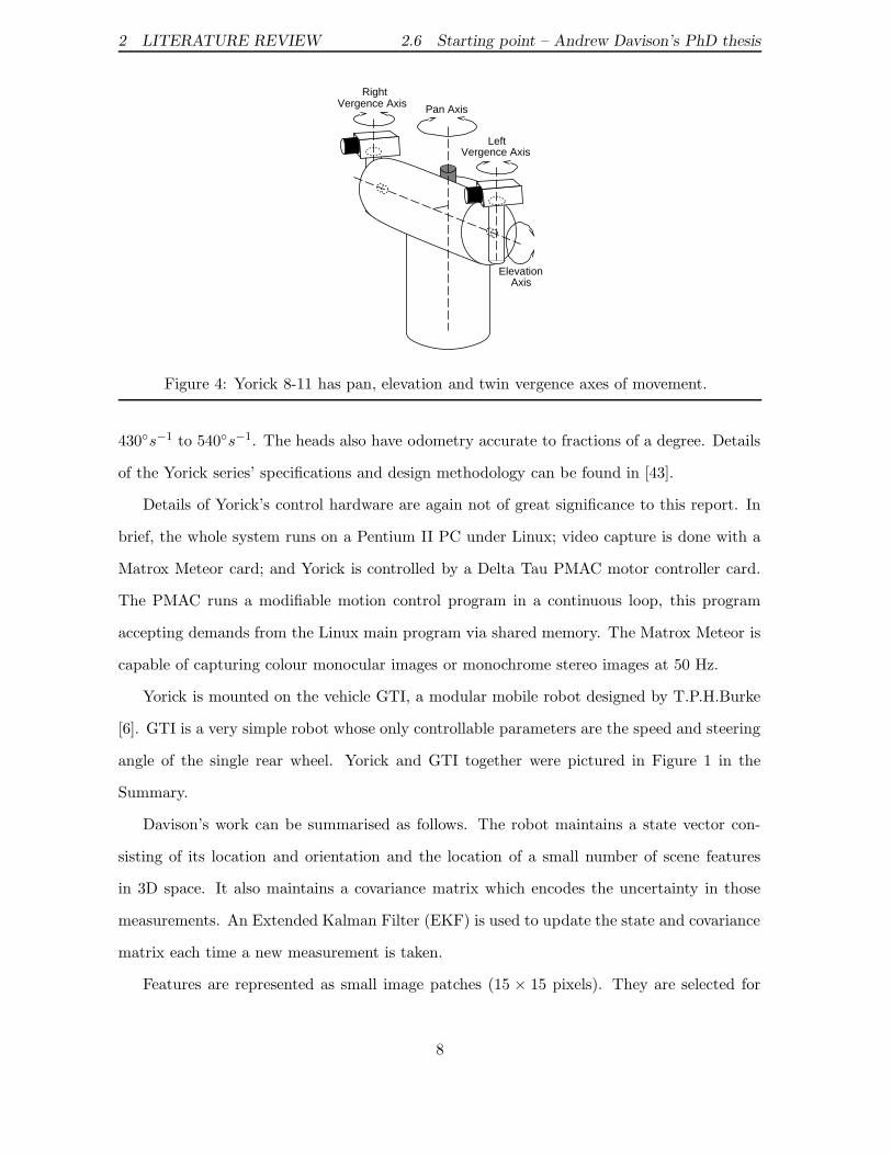
For his thesis in robot visual navigation Andrew Davison used the medium-sized Yorick 8-11
stereo pan-tilt head, pictured in Fig 2(b) in section 1. The Yorick series are of a typical
design, with common pan and elevation axes, and separate vergence axes (see Fig 4), in other
words 4 degrees of freedom as for the human visual system.
The Yorick heads were designed for high performance in tracking applications. The sort
of extreme target chosen for the design was a human sprinting across the scene at a minimum
of 2 metres from the cameras. Detailed design specifications are not relevant to this report,
but it suffices to say that the maximum accelerations of the axes ranged from 20000◦s−2 for
the pan axis to 38000◦s−2 for the vergence axes, and maximum angular velocities ranged from
7
2 LITERATURE REVIEW 2.6 Starting point – Andrew Davison’s PhD thesis
Pan Axis
ElevationAxis
LeftVergence Axis
RightVergence Axis
Figure 4: Yorick 8-11 has pan, elevation and twin vergence axes of movement.
430◦s−1 to 540◦s−1. The heads also have odometry accurate to fractions of a degree. Details
of the Yorick series’ specifications and design methodology can be found in [43].
Details of Yorick’s control hardware are again not of great significance to this report. In
brief, the whole system runs on a Pentium II PC under Linux; video capture is done with a
Matrox Meteor card; and Yorick is controlled by a Delta Tau PMAC motor controller card.
The PMAC runs a modifiable motion control program in a continuous loop, this program
accepting demands from the Linux main program via shared memory. The Matrox Meteor is
capable of capturing colour monocular images or monochrome stereo images at 50 Hz.
Yorick is mounted on the vehicle GTI, a modular mobile robot designed by T.P.H.Burke
[6]. GTI is a very simple robot whose only controllable parameters are the speed and steering
angle of the single rear wheel. Yorick and GTI together were pictured in Figure 1 in the
Summary.
Davison’s work can be summarised as follows. The robot maintains a state vector con-
sisting of its location and orientation and the location of a small number of scene features
in 3D space. It also maintains a covariance matrix which encodes the uncertainty in those
measurements. An Extended Kalman Filter (EKF) is used to update the state and covariance
matrix each time a new measurement is taken.
Features are represented as small image patches (15 × 15 pixels). They are selected for
8
2 LITERATURE REVIEW 2.6 Starting point – Andrew Davison’s PhD thesis
distinctness (large intensity variations within the patch) and for viewpoint invariance (they
are rejected if they are not easily reacquired after the robot has moved). Features are matched
in the left and right views using simple disparity matching and the constraints of the head’s
known epipolar geometry. The small number of chosen features are then fixated in turn
to obtain their 3D location by triangulation. The uncertainties of these measurements are
calculated from knowledge of uncertainty in the accuracy of fixation, of the head’s odometry,
and of the dead-reckoning procedure used to calculate the vehicle’s motion.
Between periods of fixation the robot moves according to a control law such as motion
towards, or navigation around a known target. Avoidance of obstacles not previously specified
is not possible. The robot chooses when to move, when to acquire new features, and when to
refixate old features according to higher-level decision-making processes that depend on its
location relative to known features and the uncertainty in the robot’s position estimate.
The system works well according to the limited requirement that the robot can consistently
self-localise in an unknown environment, with the uncertainty in its location bounded. The
system demonstrated this in a number of tests; for instance the robot navigated up and down
a corridor about 6m in length twice, and upon return to the start its estimated location
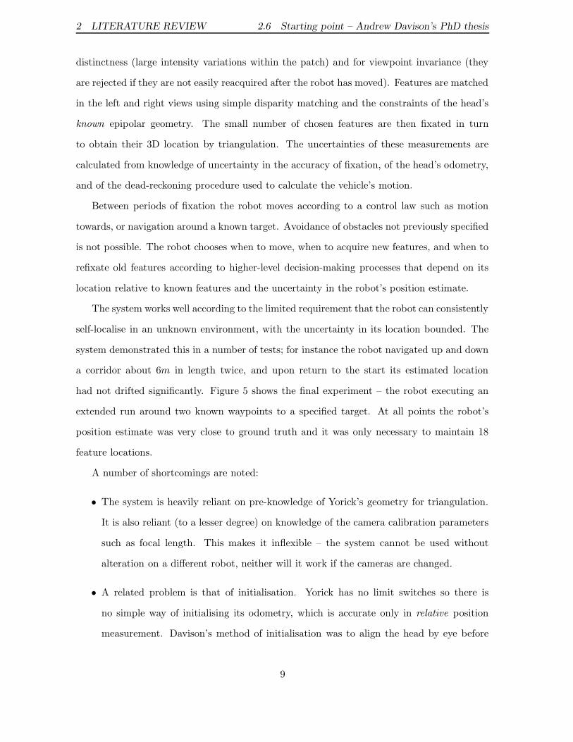
had not drifted significantly. Figure 5 shows the final experiment – the robot executing an
extended run around two known waypoints to a specified target. At all points the robot’s
position estimate was very close to ground truth and it was only necessary to maintain 18
feature locations.
A number of shortcomings are noted:
• The system is heavily reliant on pre-knowledge of Yorick’s geometry for triangulation.
It is also reliant (to a lesser degree) on knowledge of the camera calibration parameters
such as focal length. This makes it inflexible – the system cannot be used without
alteration on a different robot, neither will it work if the cameras are changed.
• A related problem is that of initialisation. Yorick has no limit switches so there is
no simple way of initialising its odometry, which is accurate only in relative position
measurement. Davison’s method of initialisation was to align the head by eye before
9

2 LITERATURE REVIEW 2.6 Starting point – Andrew Davison’s PhD thesis
x
z
0
1
Figure 5: The estimated trajectory and frames cut from a video as the robot navigatedautonomously around two known landmarks and out of the laboratory door. In the graphicaldiagram, the ellipses indicate the location and uncertainty of the scene features retained, andthe boxes the estimated location of the robot.
beginning. He estimated this to be accurate to 1 degree, possibly an underestimate.
• The system is not genuinely real-time, since the robot must pause regularly to obtain
new features and carry out the postponed EKF computation. The computation time
increases geometrically with every new feature acquired, since a new feature adds a new
row and a new column to the covariance matrix.
• The system is entirely reliant on fixation which also takes significant time since features
must be reacquired by image correlation. Unreliable camera parameters mean the robot
cannot use features that lie in the view of both cameras but are not fixated.
• The system suffers from two conflicting requirements: the need to look at right angles
to the direction of motion to take measurements which cause the greatest reduction in
the uncertainty of the robot’s location; and the need to look in the direction of motion
10

2 LITERATURE REVIEW 2.7 Conclusions
to see obstacles.
2.7 Conclusions
• There is limited literature on visual navigation of robotic vehicles.
• Fixation is known to be the main method by which humans and many other animals
navigate. Despite this, most of the work on the use of fixation in visual navigation is
the direct precursors of the work described in this report [9, 10, 35, 36].
• The literature shows that a stereo camera platform like Yorick can be easily and ac-
curately self-calibrated. Reid and Beardsley showed that such a head can also be self-
aligned at least as accurately as a manual alignment [39]. It is clear (and will be shown
in this report) that these algorithms can be extended to recover the head geometry
(that is, the positions and orientations of the rotation axes). It should also be possible
to update the information continuously during the robot’s run.
• There is considerable scope in the system for speeding up the processing and thus
enabling the robot to retain more features and so self-localise more accurately. The
current system retains more information on the relationships between each individual
features than strictly necessary, and fixation could potentially be avoided in many cases.
For instance, techniques for breaking up the map into submaps are currently being
developed at MIT [31].
11
3 NOTATION AND BASICS
3 Notation and Basics
In this section some fundamentals of projective geometry, and a few other basic mathematical
tools used in later sections are explained. For the reader’s convenience, Appendix B provides
a summary of the notation used in this report, and the important equations given here and
elsewhere.
Notation fundamentals are as follows: vectors are in bold type, 3-vectors in lower case
and 4-vectors in upper case. Matrices are in upper case teletype (as in A, B, C). In denotes
the n × n identity matrix, or I alone will be used if its dimensions are unambiguous.
3.1 Homogeneous coordinates
One of the most useful mathematical tools used in computer vision is homogeneous coordi-
nates. Vectors are extended by a single coordinate, thus, for instance, a vector represent-
ing a 2-dimensional point [x y]> is extended to [x′ y′ w]>, which can be interpreted as
x = x′/w, y = y′/w. Most of the time the choice of the additional coordinate will be arbi-
trary, or just 1; the extension is a mathematical convenience making it possible to represent
certain equations in linear matrix algebra. For instance, a euclidean transformation of a 3D
point [X Y Z]> may be represented as follows,
X ′
Y ′
Z ′
= R
XYZ
+ t
where R is the 3 × 3 rotation matrix, and t the 3 × 1 translation vector. Using homogeneous
notation the transformation may be represented by a single matrix,
X ′
Y ′
Z ′
W
=
[
R t0> 1
]
XYZ1
(1)
In this report such a transformation will be denoted matrix D. Note that homogeneous
vectors have scale invariance. Since a homogeneous vector multiplied by a scale factor still
represents the same point or line, any transformation matrix resulting in homogenous vectors
(such as D) also has arbitrary scale.
12

3 NOTATION AND BASICS 3.2 Points, lines, planes, and duality
Another useful property of homogeneous coordinates is their ability to represent points at
infinity. A 3D cartesian point at infinity can be written (X,Y,Z, 0). The point is at infinity
(X/0 = ∞ etc. ) but its direction is recorded in the ratios between X, Y and Z.
3.2 Points, lines, planes, and duality
Homogeneous coordinates are also useful in that they can be used to represent lines in 2
dimensions and planes in 3 dimensions. The equations for each are
λ1x + λ2y + λ3 = 0 (line in 2D)
Π1X + Π2Y + Π3Z + Π4 = 0 (plane in 3D)
Both are scale invariant. Thus we can represent a line in 2D in homogeneous coordinates
as λ = [λ1 λ2 λ3]>, and a plane in 3D as Π = [Π1 Π2 Π3 Π4]
>. These representations
bring about a number of useful relationships between points x and lines λ in 2D and points
X and planes Π in 3D (× represents the vector cross product):
Point on line, point on plane x>λ = 0, X>Π = 0Line through two points λ = x1 × x2
Point at intersection of two lines x = λ1 × λ2
In fact it is true to say that, in two dimensions, for any theorem of projective geometry
that applies to points there is an equivalent theorem for lines which may be derived by
interchanging the roles of points and lines. This is known as duality. In three dimensions,
points are dual to planes.
Just as there can be points at infinity, there are also lines at infinity, and a plane at
infinity. Lines at infinity are easy to visualise because horizon lines are typical examples.
The set of lines at infinity forms the plane at infinity, Π∞. In ordinary euclidean space,
Π∞ = [0 0 0 1]>. Parallel lines and parallel planes intersect on the plane at infinity, at a
vanishing point and a vanishing line respectively.
3.3 Perspective projection and camera matrices
In computer vision and photogrammetry the process by which objects in the world are mapped
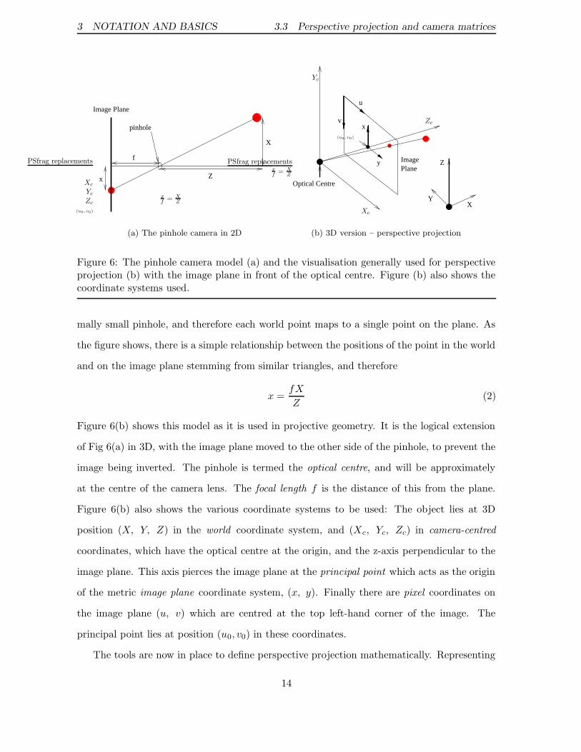
onto an image by a camera is approximated by the pinhole camera model, illustrated in Fig-
ure 6(a). Light falling on the image plane is assumed to have passed through the infinitessi-
13
3 NOTATION AND BASICS 3.3 Perspective projection and camera matrices
pinhole
x
f
X
Z
Image Plane
PSfrag replacements
xf
= XZ
Xc
Yc
Zc
(u0, v0)
(a) The pinhole camera in 2D
x
y
v
u
Optical Centre
ImagePlane
Y
Z
X
PSfrag replacementsxf
= XZ
Xc
Yc
Zc
(u0, v0)
(b) 3D version – perspective projection
Figure 6: The pinhole camera model (a) and the visualisation generally used for perspectiveprojection (b) with the image plane in front of the optical centre. Figure (b) also shows thecoordinate systems used.
mally small pinhole, and therefore each world point maps to a single point on the plane. As
the figure shows, there is a simple relationship between the positions of the point in the world
and on the image plane stemming from similar triangles, and therefore
x =fX
Z(2)
Figure 6(b) shows this model as it is used in projective geometry. It is the logical extension
of Fig 6(a) in 3D, with the image plane moved to the other side of the pinhole, to prevent the
image being inverted. The pinhole is termed the optical centre, and will be approximately
at the centre of the camera lens. The focal length f is the distance of this from the plane.
Figure 6(b) also shows the various coordinate systems to be used: The object lies at 3D
position (X, Y, Z) in the world coordinate system, and (Xc, Yc, Zc) in camera-centred
coordinates, which have the optical centre at the origin, and the z-axis perpendicular to the
image plane. This axis pierces the image plane at the principal point which acts as the origin
of the metric image plane coordinate system, (x, y). Finally there are pixel coordinates on
the image plane (u, v) which are centred at the top left-hand corner of the image. The
principal point lies at position (u0, v0) in these coordinates.
The tools are now in place to define perspective projection mathematically. Representing
14
3 NOTATION AND BASICS 3.3 Perspective projection and camera matrices
an object’s position in world coordinates, X, using homogeneous notation, we have X =
[X Y Z 1]>. This is related to its position in camera-centred coordinates, Xc by a simple
euclidean transformation, as in equation 1, so
Xc =
[
R t0> 1
]
X
A simple extension of equation 2 then provides the step from Xc to xi, the image plane
coordinates of the object (which will be a homogeneous 3-vector).
xi =
f 0 0 00 f 0 00 0 1 0
Xc
Finally, the mapping between image plane coordinates and pixel coordinates:
x =
ku 0 u0
0 kv v0
0 0 1
xi
where vector x represents the homogeneous pixel coordinates, and ku and kv are the horizontal
and vertical scale factors (converting metres to pixels). Move the factor f into this matrix to
give, overall,
x =
fku 0 u0
0 fkv v0
0 0 1
1 0 0 00 1 0 00 0 1 0
[
R t0> 1
]
X
Now put
K =
αu s u0
0 αv v0
0 0 1
(3)
where αu = fku, αv = fkv, and s = 0, and multiply out to give, in summary
x = P X = K [R t] X (4)
K is called the calibration matrix, because it encapsulates the internal parameters of the
camera. R and t encapsulate the external parameters. P is the 3 × 4 projection matrix or
camera matrix. Remember that both K and P have arbitrary scale. If P is known then the
camera is said to be calibrated. However the world coordinate system is usually arbitrarily
chosen and thus can be set the same as the camera-centred system. In this case P = K [I 0],
and camera calibration involves finding K only.
This model suffices in most cases although some modifications often made are
15
3 NOTATION AND BASICS 3.4 3-space and non-metric structure
• s in equation 3 is non-zero. s encodes skew, or the non-orthogonality of rows and
columns in the image. s is usually very close to zero, but in this work it suffices to
assume that K is a general upper-triangular matrix with 5 degrees of freedom (6− 1 for
arbitrary scale).
• Lens imperfection and misalignment cause two types of distortion of the image. One,
radial distortion, increases with distance from the principal point; the other, tangential
distortion, varies with direction from it. Tangential distortion is always minimal but
radial distortion is significant in all but high quality cameras.
Although the P matrix has a specific form it is often taken to be a general 3 × 4 matrix
with 11 degrees of freedom. This means it can be used to project non-metric structure, as
explained in the next section.
3.4 3-space and non-metric structure
3 dimensional space, or 3-space, is defined by the types of transformations that are allowed
on objects in the space. In the 3-space commonly understood, known as metric or euclidean
space, these are euclidean euclidean transformations, represented by the matrix D of equation
1 acting on homogeneous coordinates. It has six degrees of freedom, 3 for the rotation, 3 for
the translation, and thus the motion of 3 points defines the motion for all points.
If the transformation matrix is allowed to be completely general, it has 15 degrees of
freedom (arbitrary scale), and 5 points are needed to define it. More importantly, such a
transformation allows up to 5 points to be moved to arbitrary locations. This transformation
is called a projective transformation, because it distorts objects in a similar way to perspective
projection. Projective transformations allow objects to scale and shear in all directions and
cause parallel lines to converge to a vanishing point. Thus it can bring points from infinity to
real locations. There is also affine space, which maintains points at infinity but allows shear
and scaling. An affine tranformation has the form A =
[
A t0> 1
]
where A is a general 3 × 3
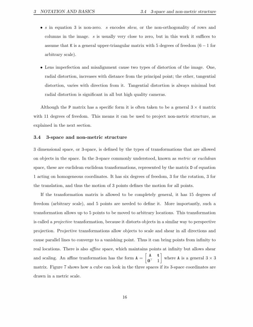
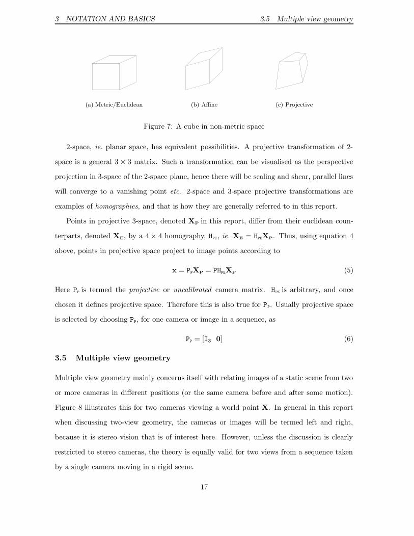
matrix. Figure 7 shows how a cube can look in the three spaces if its 3-space coordinates are
drawn in a metric scale.
16
3 NOTATION AND BASICS 3.5 Multiple view geometry
(a) Metric/Euclidean (b) Affine (c) Projective
Figure 7: A cube in non-metric space
2-space, ie. planar space, has equivalent possibilities. A projective transformation of 2-
space is a general 3 × 3 matrix. Such a transformation can be visualised as the perspective
projection in 3-space of the 2-space plane, hence there will be scaling and shear, parallel lines
will converge to a vanishing point etc. 2-space and 3-space projective transformations are
examples of homographies, and that is how they are generally referred to in this report.
Points in projective 3-space, denoted XP in this report, differ from their euclidean coun-
terparts, denoted XE, by a 4 × 4 homography, HPE, ie. XE = HPEXP. Thus, using equation 4
above, points in projective space project to image points according to
x = PPXP = PHPEXP (5)
Here PP is termed the projective or uncalibrated camera matrix. HPE is arbitrary, and once
chosen it defines projective space. Therefore this is also true for PP. Usually projective space
is selected by choosing PP, for one camera or image in a sequence, as
PP = [I3 0] (6)
3.5 Multiple view geometry
Multiple view geometry mainly concerns itself with relating images of a static scene from two
or more cameras in different positions (or the same camera before and after some motion).
Figure 8 illustrates this for two cameras viewing a world point X. In general in this report
when discussing two-view geometry, the cameras or images will be termed left and right,
because it is stereo vision that is of interest here. However, unless the discussion is clearly
restricted to stereo cameras, the theory is equally valid for two views from a sequence taken
by a single camera moving in a rigid scene.
17
3 NOTATION AND BASICS 3.5 Multiple view geometry
PSfrag replacementsC C′
e e′
x x′
l l′
R
t
X
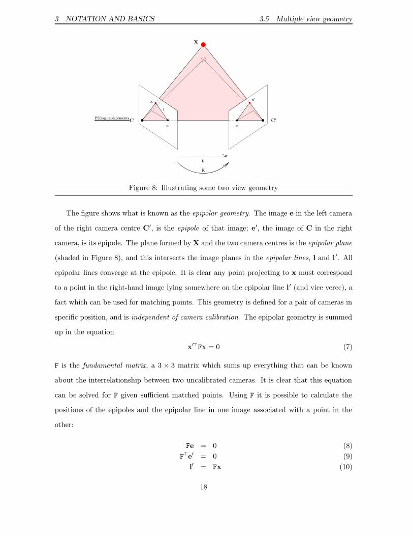
Figure 8: Illustrating some two view geometry
The figure shows what is known as the epipolar geometry. The image e in the left camera
of the right camera centre C′, is the epipole of that image; e′, the image of C in the right
camera, is its epipole. The plane formed by X and the two camera centres is the epipolar plane
(shaded in Figure 8), and this intersects the image planes in the epipolar lines, l and l ′. All
epipolar lines converge at the epipole. It is clear any point projecting to x must correspond
to a point in the right-hand image lying somewhere on the epipolar line l′ (and vice verce), a
fact which can be used for matching points. This geometry is defined for a pair of cameras in
specific position, and is independent of camera calibration. The epipolar geometry is summed
up in the equation
x′>Fx = 0 (7)
F is the fundamental matrix, a 3 × 3 matrix which sums up everything that can be known
about the interrelationship between two uncalibrated cameras. It is clear that this equation
can be solved for F given sufficient matched points. Using F it is possible to calculate the
positions of the epipoles and the epipolar line in one image associated with a point in the
other:
Fe = 0 (8)
F>e′ = 0 (9)
l′ = Fx (10)
18
3 NOTATION AND BASICS 3.6 Algorithms
l = F>x′ (11)
Equations 8 and 9 show that F is rank-deficient. This, combined with the matrix’s scale
invariance common to all operators in projective geometry (§3.1), means that the fundamental
matrix has only 7 degrees of freedom, so only 7 point matches are required to define it.
In addition, if one camera matrix is chosen to be [I 0] as in equation 6, the other will be
given by
P′P= [(e′ × F) e′] (12)
where e′ is the right image epipole, the null space of F> (equation 9).
The fundamental matrix is unfortunately not sufficient for representing all situations. If
the scene features all lie on a single plane, or t in Figure 8 is zero (there is only a rotation
between the cameras), then the fundamental matrix is undefined or not unique, and there is
a unique mapping from one image plane to the other. This mapping is a 3 × 3 homography.
These situations are termed degenerate. Degeneracy causes numerical problems with calcu-
lating the fundamental matrix even when the scene is close to planar, or the translation t
is simply small compared with scene distance. Degenerate conditions mean that projection
matrices (and therefore projective structure) cannot be extracted from a pair of views.
3.6 Algorithms
There are a few techniques commonly used in projective geometry for matching feature points
in images and using them to calculate and refine matrices. Much of the work described in this
report involves the use of algorithms that are becoming the standard, and they are briefly
described in this section. Not explained is the Harris corner detector, the algorithm used for
locating viewpoint invariant interest points in an image. The Harris detector selects points
of high intensity gradient in both horizontal and vertical directions – the reader is referred to
[19].
3.6.1 Disparity matching
Once a number of interest points have been found in two images, it is necessary to match up as
many of them as possible. A disparity matcher searches in a circular region in a second image
19
3 NOTATION AND BASICS 3.6 Algorithms
around the location of a feature in the first, for points of similar local intensity variation.
3.6.2 The Direct Linear Transform
Any linear relationship can be reformulated as a null vector problem, i.e. that of finding the
solution n to Mn = 0 where M is a design matrix. For instance, in the case of the fundamental
matrix, we have (equation 7)
[ x′ y′ 1 ]
f1 f2 f3
f4 f5 f6
f7 f8 f9
xy1
= 0
⇒ [ x′x x′y x′ y′x y′y y′ x y 1 ]
f1
f2
f3
f4
f5
f6
f7
f8
f9
= 0 (13)
This is true for all matched pairs of points, so N vectors on the left of equation 13 can be
stacked up to form an N × 9 design matrix M, with the right-hand vector f as its null space.
Because the point positions will not be exactly accurate, it is desirable for N to be as
large as possible to provide a solution f for which equation 13 is as close to zero as possible
for all points. The Direct Linear Transform (DLT) does this, by least-squares minimisation of
the algrebraic error, ‖Mf‖/‖f‖. Simply take the eigenvector of M>M with least eigenvalue. This
procedure is linear, and therefore fast. Usually it is done using the Singular Value Decompo-
sition (SVD) which decomposes M as M = UΣV>, with Σ diagonal and U and V orthonormal.
The vector required will be the rightmost column of V.
3.6.3 RANSAC
Disparity matching and the DLT alone are useless. At least 10% of the matches are likely to
be incorrect, and the DLT is very sensitive to the presence of data that doesn’t fit the model,
or outliers. Just one or two outliers can lead to invalid results.
RANSAC, or RANdom Sampling And Consensus, will remove outliers from a set of puta-
tive matches. RANSAC randomly selects a sample of the minimum number of point matches
20
3 NOTATION AND BASICS 3.6 Algorithms
needed to calculate a solution from the seed set provided by the disparity matcher (7 for a
fundamental matrix). Then it tests how well this solution fits the rest of the seed set. The
procedure iterates until as many good matches are found as possible, then these matches are
retained and the rest discarded as outliers. Thus RANSAC terminates with a good solution
and set of matches with minimal outliers. In practice RANSAC terminates after a maximum
number of iterations, when the percentage of inliers reaches an expected value, or when the
probability of finding a larger set of inliers drops below a threshold.
3.6.4 Non-linear minimisation and bundle adjustment
The final stage could be to use the DLT with all the inlying points to get a better solution, but
the DLT minimises an algebraic error when really we want to reduce a metric error. Ideally
the solution should minimise transfer error (usually referred to as reprojection error, which is
technically incorrect since this refers to a slightly different metric), the distance in the image
between a point match and its counterpart transferred into its image. This can be done using
a non-linear minimisation routine. The routine used for this project is Levenberg-Marquardt
Iteration, which is not described here. Suffice to say it is a commonly used, accurate, and fast
technique for finding the solution to non-linear equations. The routine is provided with an
initial solution and told how to calculate the error from it. It then makes iterative alterations
to the solution to minimise the error. For further information see [21]. The DLT can be used
to initialise the procedure.
However, many points that could be matched that were not found by the disparity matcher
have been left out. The solution can be used to carry out guided matching on the entire data
set. That is, points can be matched to others that fit the solution well. This provides many
more matches which can then be used to refine the solution further. This bundle adjustment
cycle continues, usually stopping when further iterations no longer change the set of inliers.
Sometimes it is a good idea to include RANSAC in the loop – outliers not detected in the
first run can consequently fail to be detected at this stage yet entirely invalidate the result.
21

3 NOTATION AND BASICS 3.6 Algorithms
3.6.5 Summary of two view matching procedure
The following summarises the standard procedure for a two view fundamental matrix or
homography calculation, and gives some typical results.
1. Harris corner detection. Gives about 600 corners per image.
2. Disparity matching. About 200 putative matches.
3. RANSAC. About 100 inliers.
4. Bundle adjustment. The final inlier count will hopefully be 200-300 matches. Less than
100 matches would suggest the accuracy of the result was poor.
For two 768 × 576 images, the whole procedure will take 30 seconds to a minute on a fast
Pentium II PC.
22

4 ALIGNING THE ELEVATION AND VERGENCE
4 Aligning the Elevation and Vergence
About two-thirds of this year’s work has been on this part of the robot’s self-initialisation.
The original self-alignment work was done by Reid and Beardsley [39], and was implemented,
and shown to work both in theory and in limited cases in practice. The task for this project
was to reimplement the procedure and try and get it to work in as many situations as pos-
sible. This led to some considerable work on robust calculation and new theory on how to
handle degeneracy. This section explains the theory in detail and goes on to discuss practical
implementation of the procedure, and to look at the results. Refer to Appendix B for any
equations referenced.
4.1 Theory
4.1.1 Groundwork
We examine a Euclidean transformation D of homogeneous 3D point space, as defined in §3.1.
D acts on euclidean points XE taking them to X′
E, so X′
E= DXE. Points in 3D projective
space are represented by XP and X′
P, where projective space and euclidean space are related
by update matrix HPE s. t. XE = HPEXP (as in §3.4). From this we find the form of projective
transformation H, where X′
P= HXP, as
H = H−1
PEDHPE (14)
We call this the general case. More specifically, we are also interested in the limited case where
D is itself conjugate to a rotation alone. This occurs where the transformation is a rotation
about an axis that does not pass through the origin, equivalent to t being perpendicular to
that axis. In this case,
D = D−1
tR3DDt =
[
Rt tt0> 1
]
−1
cos θ − sin θ 0 0sin θ cos θ 0 0
0 0 1 00 0 0 1
[
Rt tt0> 1
]
(15)
Here, Dt is the transformation that takes the z-axis to the axis of rotation, and θ is the angle of
rotation about that axis. Any euclidean transformation is equivalent to a rotation about, and
translation along an axis in 3-space, called the screw. This situation occurs when a camera
23
4 ALIGNING THE ELEVATION AND VERGENCE 4.1 Theory
head makes a rotation about one of its axes alone, meaning the translation component (the
pitch of the screw) is zero.
4.1.2 Identifying HPE
It is now well known that for two views of a scene where one camera has internal parameter
matrix K,
HPE =
[
K−1 0a> d
]
(16)
where [a> d]> is the plane at infinity in projective space, Π∞P.
To prove equation 16, put HPE =
[
E fg> h
]
. Equation 5 showed that PP = PHPE. Choose
PP = [I 0] as we may, and choose to align the world coordinate system with one camera’s
coordinate system. It follows that
[I 0] = K[I 0]
[
E fg> h
]
⇒ [I 0] = [KE f ]
which proves the top 3 × 4 block of HPE. Now, points are taken from euclidean to projective
space by H−1
PE. Thus planes are taken from euclidean to projective space by its dual, which is
H>
PE(not proved here, but see eg. [21]). Thus,
Π∞P =
[
ad
]
= H>
PEΠ∞ = H>
PE
0001
=
[
K−1 g0> h
]
0001
=
[
gh
]
which completes proof of (16). Note that K in this case will be the calibration matrix of
whichever camera was chosen as the centre of the world coordinate system, not necessarily that
of any other camera. The projective camera matrix of another view, P′P, can be calculated from
point correspondences (equation 12), and the corresponding calibrated matrix P ′ = P′PH−1
PE.
We know P′ = [P′ p′] = K′[R′ t′] so K′ and R′, and therefore t′ can be extracted by QR
decomposition of P′−1.
4.1.3 The Non-degenerate case
Zisserman et al. [49], Reid & Beardsley [39], and others [1, 3] showed that for a euclidean or
conjugate euclidean transformation H = H−1
PEDHPE, there is a fixed line on the plane at infinity
24
4 ALIGNING THE ELEVATION AND VERGENCE 4.1 Theory
Screw axisPSfrag replacements
Π∞
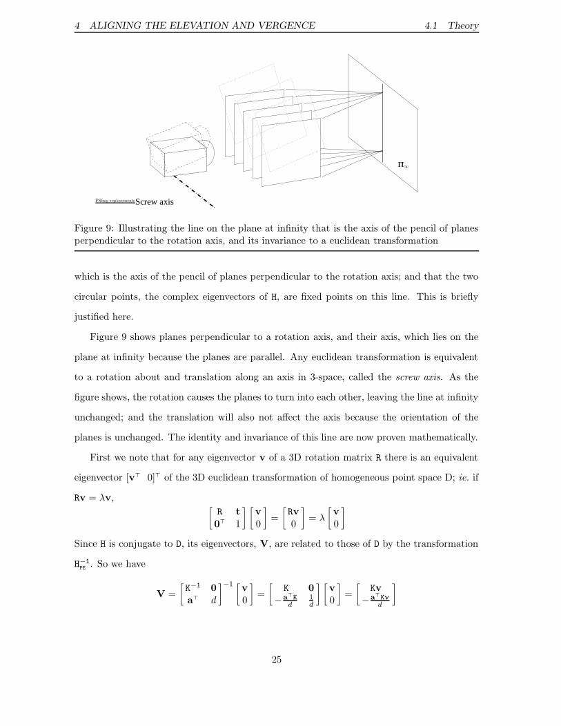
Figure 9: Illustrating the line on the plane at infinity that is the axis of the pencil of planesperpendicular to the rotation axis, and its invariance to a euclidean transformation
which is the axis of the pencil of planes perpendicular to the rotation axis; and that the two
circular points, the complex eigenvectors of H, are fixed points on this line. This is briefly
justified here.
Figure 9 shows planes perpendicular to a rotation axis, and their axis, which lies on the
plane at infinity because the planes are parallel. Any euclidean transformation is equivalent
to a rotation about and translation along an axis in 3-space, called the screw axis. As the
figure shows, the rotation causes the planes to turn into each other, leaving the line at infinity
unchanged; and the translation will also not affect the axis because the orientation of the
planes is unchanged. The identity and invariance of this line are now proven mathematically.
First we note that for any eigenvector v of a 3D rotation matrix R there is an equivalent
eigenvector [v> 0]> of the 3D euclidean transformation of homogeneous point space D; ie. if
Rv = λv,[
R t0> 1
] [
v0
]
=
[
Rv0
]
= λ
[
v0
]
Since H is conjugate to D, its eigenvectors, V, are related to those of D by the transformation
H−1
PE. So we have
V =
[
K−1 0a> d
]
−1 [v0
]
=
[
K 0−a
>K
d1
d
] [
v0
]
=
[
Kv−a
>Kv
d
]
25
4 ALIGNING THE ELEVATION AND VERGENCE 4.1 Theory
thus we can write
Π>
∞PV = [a> d]
[
Kv−a
>Kv
d
]
= a>Kv − a>Kv = 0
which proves that three of the eigenvectors of H are points on the plane at infinity. Two of
the eigenvectors of R will be complex and thus we can be sure that V3 and V4, the complex
eigenvectors of H, or circular points, lie on Π∞. The line between these points, which may
be represented by αV3 + βV4, is a fixed line since any point on it remains on the line under
the transformation (H(αV3 + βV4) = λ3αV3 + λ4βV4, where λ3 and λ4 are the eigenvalues
associated with V3 and V4).
The real eigenvector of R is the direction of the axis of rotation, and the eigenvector of H
associated with this, V1, is the point at which this direction meets the plane at infinity.It is
clear from the geometry of Figure 9 that this direction is perpendicular to the invariant line
at infinity.
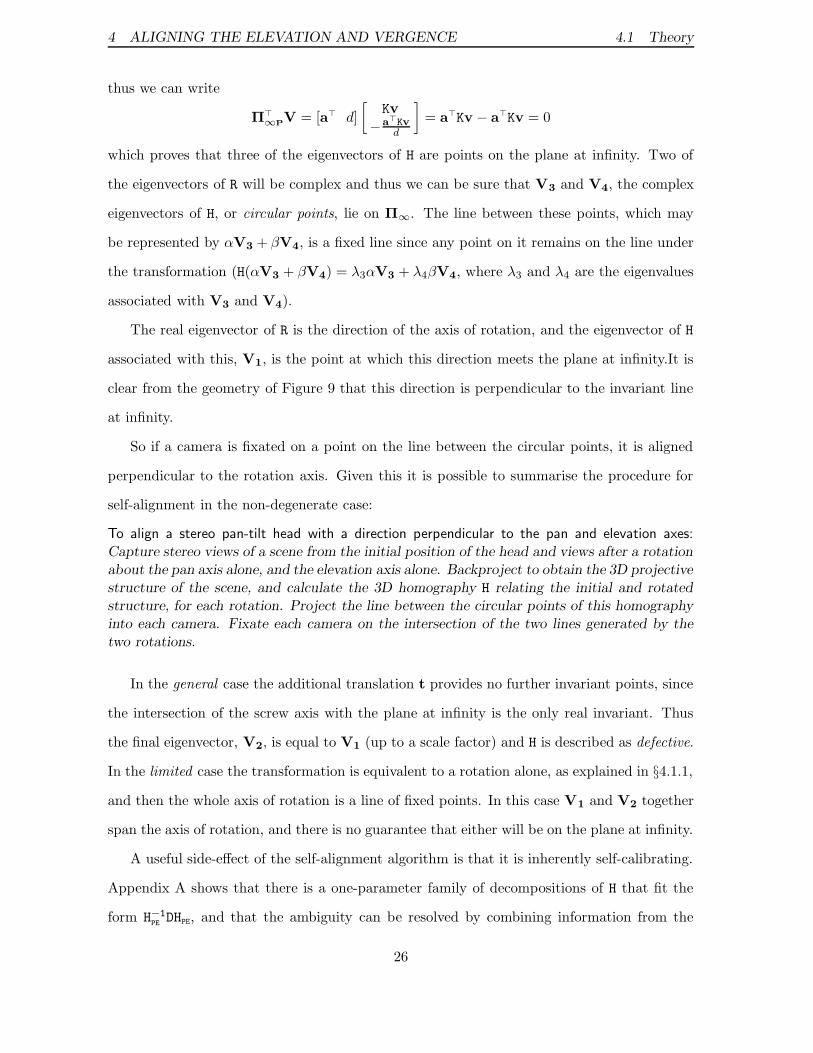
So if a camera is fixated on a point on the line between the circular points, it is aligned
perpendicular to the rotation axis. Given this it is possible to summarise the procedure for
self-alignment in the non-degenerate case:
To align a stereo pan-tilt head with a direction perpendicular to the pan and elevation axes:
Capture stereo views of a scene from the initial position of the head and views after a rotation
about the pan axis alone, and the elevation axis alone. Backproject to obtain the 3D projective
structure of the scene, and calculate the 3D homography H relating the initial and rotated
structure, for each rotation. Project the line between the circular points of this homography
into each camera. Fixate each camera on the intersection of the two lines generated by the
two rotations.
In the general case the additional translation t provides no further invariant points, since
the intersection of the screw axis with the plane at infinity is the only real invariant. Thus
the final eigenvector, V2, is equal to V1 (up to a scale factor) and H is described as defective.
In the limited case the transformation is equivalent to a rotation alone, as explained in §4.1.1,
and then the whole axis of rotation is a line of fixed points. In this case V1 and V2 together
span the axis of rotation, and there is no guarantee that either will be on the plane at infinity.
A useful side-effect of the self-alignment algorithm is that it is inherently self-calibrating.
Appendix A shows that there is a one-parameter family of decompositions of H that fit the
form H−1
PEDHPE, and that the ambiguity can be resolved by combining information from the
26
4 ALIGNING THE ELEVATION AND VERGENCE 4.1 Theory
two rotations about the different head axes. It is therefore possible to obtain the matrix
HPE unambiguously and therefore the calibration matrix K. Knowledge of D for each rotation
provides the locations of the rotation axes (or location in the limited case, direction only
in the general case), as explained. This means that Yorick can be self-aligned and self-
calibrated entirely automatically with just two rotations, a complete self-initialisation. In
practice the calibration from two rotations is likely to be poor quality, but it can be updated
from correspondences obtained during the robot’s motion.
4.1.4 The degenerate case
Degeneracy of the homography H can occur in two ways as explained in section 3.5. In
either case the initial and rotated views of the scene in one camera are related by a 2D
homography which we denote H2D. If the scene structure is planar, projective structure can
still be calculated by rotating the head about the combined axes, combining point matches
from the different views, and using them to calculate the fundamental matrix. In practice,
however, the off-plane structure generated by such motions will be too small to calculate
a good F, so to state that projective structure cannot be calculated is reasonably fair. If
degeneracy is caused by a pure rotation relating left and right views, projective structure can
genuinely not be calculated from any number of views.
In either case the projective structure and homography H still exist, they merely cannot
be calculated. To solve this problem we utilise a motion constraint, that is, when the head
rotates about a single axis it is undergoing zero-pitch screw rotation as explained in §3.1.
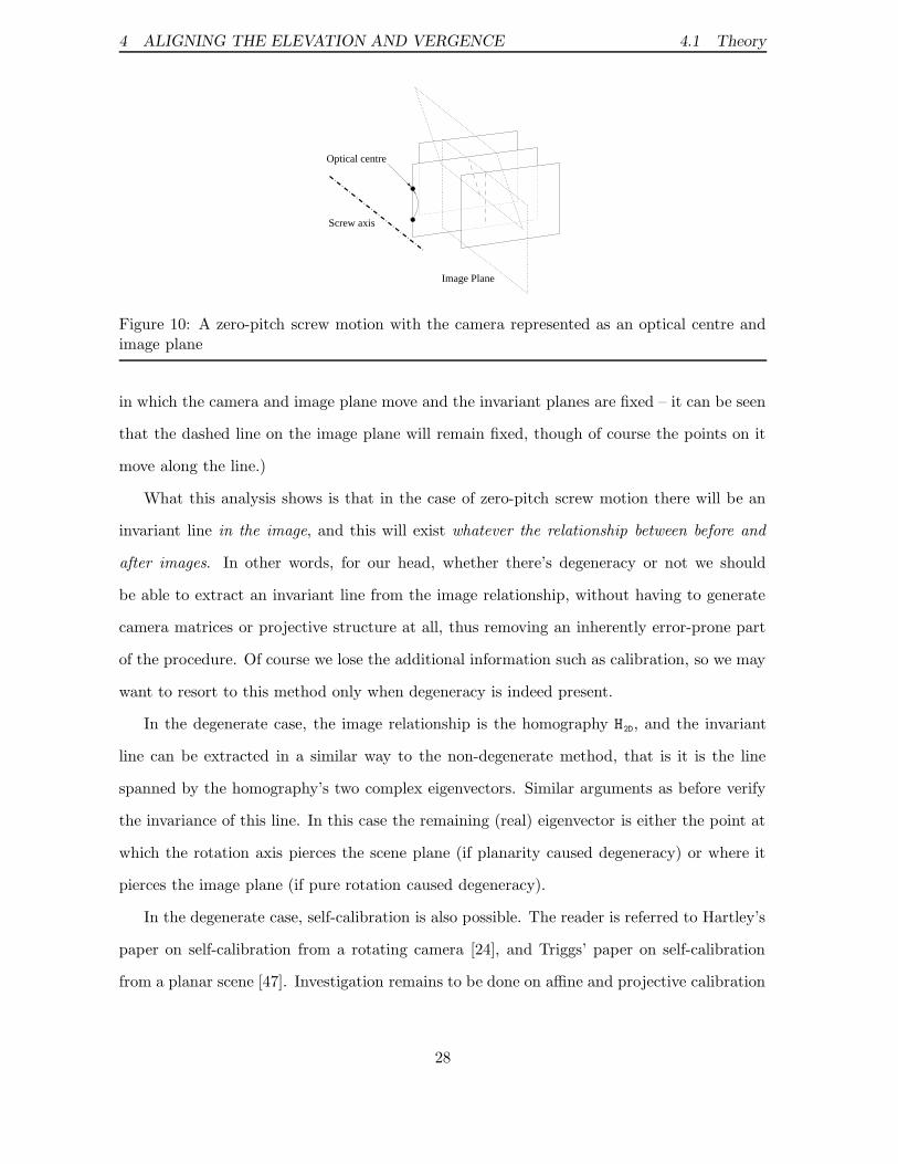
Figure 10 shows a camera undergoing the same motion as in Figure 9, this time with the
camera represented as an optical centre and image plane. The three parallel planes are the
planes invariant to the motion, whose axis is the invariant line that was calculated in the
non-degenerate case. By the rules of central projection this line at infinity projects to the
image plane at the line dashed in the figure; this is equivalently the intersection of the specific
invariant plane which passes through the optical centre, and the image plane. In the case of
zero-pitch screw motion this plane rotates into itself (which is why it is invariant), and thus
the intersection remains the same line on the image plane. (The figure shows the equivalent,
27
4 ALIGNING THE ELEVATION AND VERGENCE 4.1 Theory
Screw axis
Optical centre
Image Plane
Figure 10: A zero-pitch screw motion with the camera represented as an optical centre andimage plane
in which the camera and image plane move and the invariant planes are fixed – it can be seen
that the dashed line on the image plane will remain fixed, though of course the points on it
move along the line.)
What this analysis shows is that in the case of zero-pitch screw motion there will be an
invariant line in the image, and this will exist whatever the relationship between before and
after images. In other words, for our head, whether there’s degeneracy or not we should
be able to extract an invariant line from the image relationship, without having to generate
camera matrices or projective structure at all, thus removing an inherently error-prone part
of the procedure. Of course we lose the additional information such as calibration, so we may
want to resort to this method only when degeneracy is indeed present.
In the degenerate case, the image relationship is the homography H2D, and the invariant
line can be extracted in a similar way to the non-degenerate method, that is it is the line
spanned by the homography’s two complex eigenvectors. Similar arguments as before verify
the invariance of this line. In this case the remaining (real) eigenvector is either the point at
which the rotation axis pierces the scene plane (if planarity caused degeneracy) or where it
pierces the image plane (if pure rotation caused degeneracy).
In the degenerate case, self-calibration is also possible. The reader is referred to Hartley’s
paper on self-calibration from a rotating camera [24], and Triggs’ paper on self-calibration
from a planar scene [47]. Investigation remains to be done on affine and projective calibration
28
4 ALIGNING THE ELEVATION AND VERGENCE 4.1 Theory
in the degenerate case for stereo views using controlled rotations about the head axes.
It is important to note that the degeneracy applies for degeneracy between views before
and after a rotation, not between left and right cameras. Those two views can be related by
a 2D homography even if left and right images are not. In fact, this is very likely since for a
small rotation, the translational component is likely to be small. In this case, either of the
two algorithms can be used. Possibly the degenerate case should be favoured, since it is faster
and results in more point matches, which benefits accuracy. However, the self-calibration will
be less accurate.
4.1.5 Fixating with zero knowledge
Fixating a point in each camera sounds simple, but even with calibrated cameras it is not
necessarily straightforward, because the head rotation axes do not pass through the camera
optical centres.
The calibration information is not available until after the second rotation, and even then
it will be unreliable. The best solution is to make some simple assumptions and then use image
correlation to refind the fixation point and make small adjustments. Assume the camera has
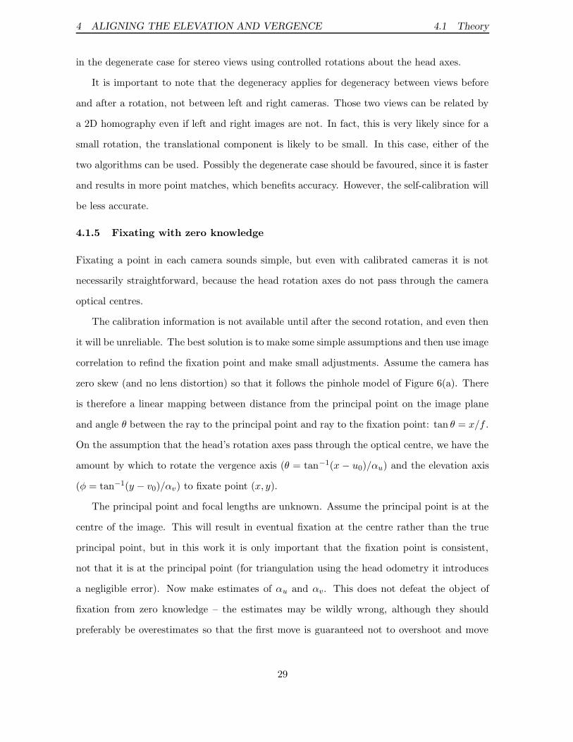
zero skew (and no lens distortion) so that it follows the pinhole model of Figure 6(a). There
is therefore a linear mapping between distance from the principal point on the image plane
and angle θ between the ray to the principal point and ray to the fixation point: tan θ = x/f .
On the assumption that the head’s rotation axes pass through the optical centre, we have the
amount by which to rotate the vergence axis (θ = tan−1(x − u0)/αu) and the elevation axis
(φ = tan−1(y − v0)/αv) to fixate point (x, y).
The principal point and focal lengths are unknown. Assume the principal point is at the
centre of the image. This will result in eventual fixation at the centre rather than the true
principal point, but in this work it is only important that the fixation point is consistent,
not that it is at the principal point (for triangulation using the head odometry it introduces
a negligible error). Now make estimates of αu and αv. This does not defeat the object of
fixation from zero knowledge – the estimates may be wildly wrong, although they should
preferably be overestimates so that the first move is guaranteed not to overshoot and move
29
4 ALIGNING THE ELEVATION AND VERGENCE 4.2 Implementation
the fixation point off the image. Calculate the rotation angles, move the head, and refind the
fixation point in the image using some correlation technique. Use the new location and the
angles moved to adjust the α values, and continue iterating until fixation is complete.
If the fixation point is initially off the image, correlation cannot be performed on the
fixation point, so instead fixate the cameras on a point near the edge of the image. Doing so
should provide sufficiently accurate values of αu and αv to bring the required fixation point
within the image. Then the auto-alignment algorithm can be repeated.
4.2 Implementation
The self-alignment theory is sound, and this is proven by the experiments with simulated
data shown in §4.3. But in practice there are many implementation issues that are important
for enabling the alignment to work in a large variety of circumstances. Mostly they are to do
with obtaining sufficient feature matches between views to calculate accurate relationships.
This section outlines the algorithms used for the elements of self-alignment, and discusses
possible alterations for improvement.
The algorithms for establishing two view relationships have not been layed out in detail,
since commonly available and highly reliable ones were used that follow the pattern of section
3.6.5.
In this section, the term image refers either to a particular image, specifically the left or
right image of a stereo view. The term view is used to discriminate between stereo views
before and after a head rotation. Similarly the superscripts l and r represent left and right,
whereas prime (′) represents a rotated view (or superscripts c, e and p for central, elevated,
and panned views, described later).
4.2.1 Non-degenerate case
This is the hardest algorithm to implement because it requires feature matching between four
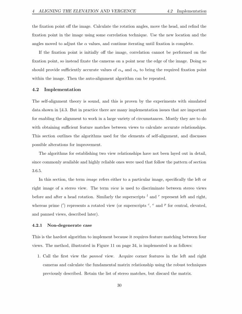
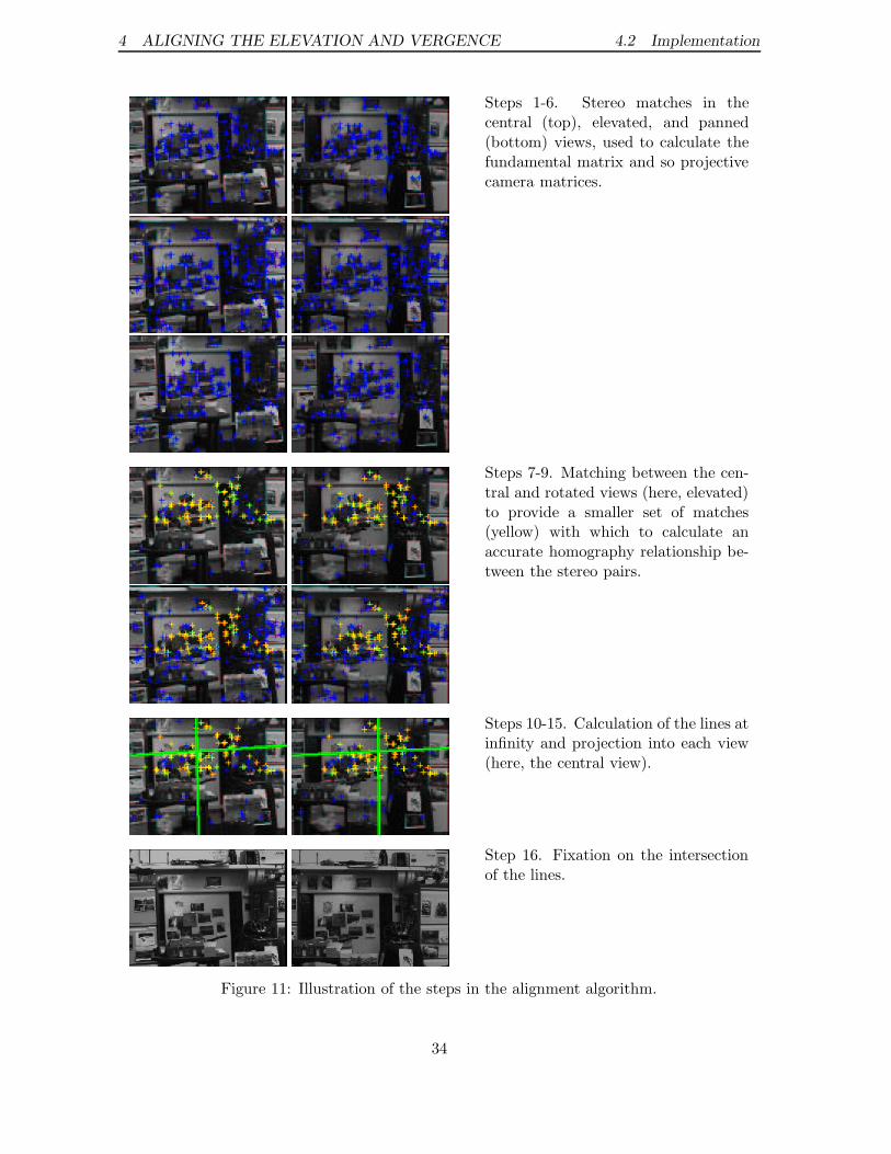
views. The method, illustrated in Figure 11 on page 34, is implemented is as follows:
1. Call the first view the panned view. Acquire corner features in the left and right
cameras and calculate the fundamental matrix relationship using the robust techniques
previously described. Retain the list of stereo matches, but discard the matrix.
30
4 ALIGNING THE ELEVATION AND VERGENCE 4.2 Implementation
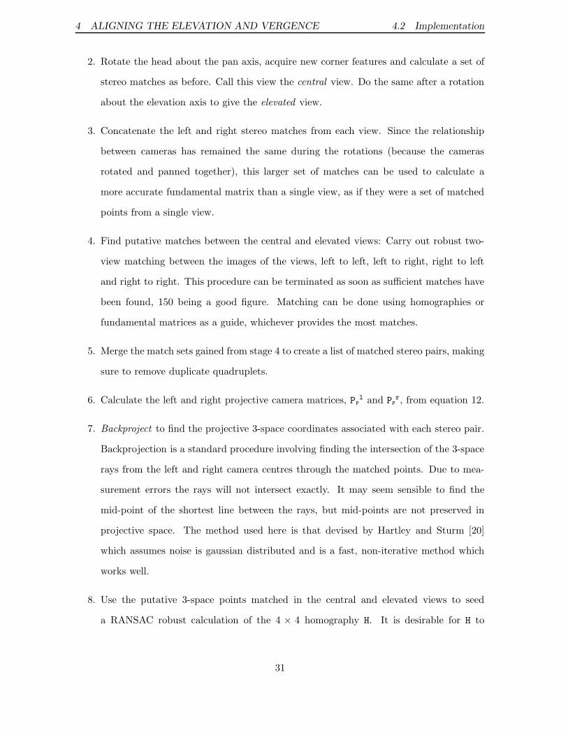
2. Rotate the head about the pan axis, acquire new corner features and calculate a set of
stereo matches as before. Call this view the central view. Do the same after a rotation
about the elevation axis to give the elevated view.
3. Concatenate the left and right stereo matches from each view. Since the relationship
between cameras has remained the same during the rotations (because the cameras
rotated and panned together), this larger set of matches can be used to calculate a
more accurate fundamental matrix than a single view, as if they were a set of matched
points from a single view.
4. Find putative matches between the central and elevated views: Carry out robust two-
view matching between the images of the views, left to left, left to right, right to left
and right to right. This procedure can be terminated as soon as sufficient matches have
been found, 150 being a good figure. Matching can be done using homographies or
fundamental matrices as a guide, whichever provides the most matches.
5. Merge the match sets gained from stage 4 to create a list of matched stereo pairs, making
sure to remove duplicate quadruplets.
6. Calculate the left and right projective camera matrices, PP
l and PP
r, from equation 12.
7. Backproject to find the projective 3-space coordinates associated with each stereo pair.
Backprojection is a standard procedure involving finding the intersection of the 3-space
rays from the left and right camera centres through the matched points. Due to mea-
surement errors the rays will not intersect exactly. It may seem sensible to find the
mid-point of the shortest line between the rays, but mid-points are not preserved in
projective space. The method used here is that devised by Hartley and Sturm [20]
which assumes noise is gaussian distributed and is a fast, non-iterative method which
works well.
8. Use the putative 3-space points matched in the central and elevated views to seed
a RANSAC robust calculation of the 4 × 4 homography H. It is desirable for H to
31
4 ALIGNING THE ELEVATION AND VERGENCE 4.2 Implementation
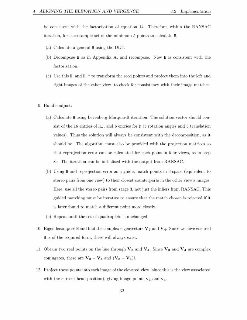
be consistent with the factorisation of equation 14. Therefore, within the RANSAC
iteration, for each sample set of the minimum 5 points to calculate H,
(a) Calculate a general H using the DLT.
(b) Decompose H as in Appendix A, and recompose. Now H is consistent with the
factorisation.
(c) Use this H, and H−1 to transform the seed points and project them into the left and
right images of the other view, to check for consistency with their image matches.
9. Bundle adjust:
(a) Calculate H using Levenberg-Marquardt iteration. The solution vector should con-
sist of the 16 entries of HPE, and 6 entries for D (3 rotation angles and 3 translation
values). Thus the solution will always be consistent with the decomposition, as it
should be. The algorithm must also be provided with the projection matrices so
that reprojection error can be calculated for each point in four views, as in step
8c. The iteration can be initialised with the output from RANSAC.
(b) Using H and reprojection error as a guide, match points in 3-space (equivalent to
stereo pairs from one view) to their closest counterparts in the other view’s images.
Here, use all the stereo pairs from stage 3, not just the inliers from RANSAC. This
guided matching must be iterative to ensure that the match chosen is rejected if it
is later found to match a different point more closely.
(c) Repeat until the set of quadruplets is unchanged.
10. Eigendecompose H and find the complex eigenvectors V3 and V4. Since we have ensured
H is of the required form, these will always exist.
11. Obtain two real points on the line through V3 and V4. Since V3 and V4 are complex
conjugates, these are V3 + V4 and (V3 −V4)i.
12. Project these points into each image of the elevated view (since this is the view associated
with the current head position), giving image points v3 and v4.
32
4 ALIGNING THE ELEVATION AND VERGENCE 4.2 Implementation
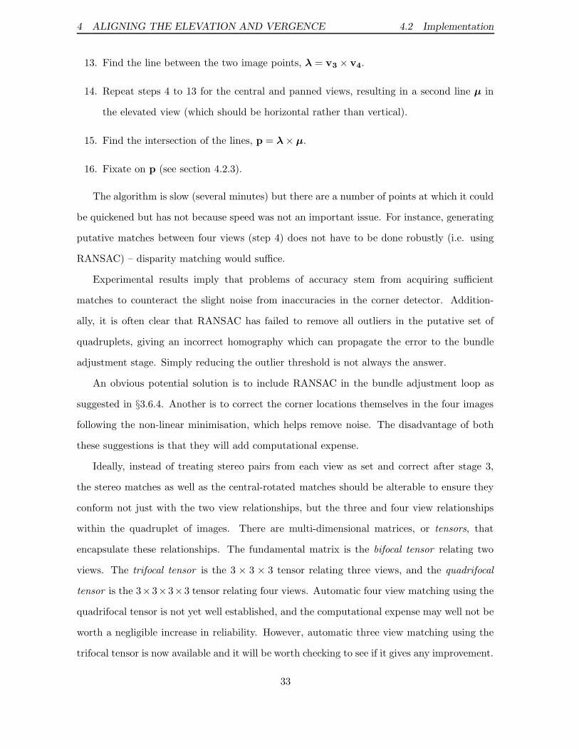
13. Find the line between the two image points, λ = v3 × v4.
14. Repeat steps 4 to 13 for the central and panned views, resulting in a second line µ in
the elevated view (which should be horizontal rather than vertical).
15. Find the intersection of the lines, p = λ × µ.
16. Fixate on p (see section 4.2.3).
The algorithm is slow (several minutes) but there are a number of points at which it could
be quickened but has not because speed was not an important issue. For instance, generating
putative matches between four views (step 4) does not have to be done robustly (i.e. using
RANSAC) – disparity matching would suffice.
Experimental results imply that problems of accuracy stem from acquiring sufficient
matches to counteract the slight noise from inaccuracies in the corner detector. Addition-
ally, it is often clear that RANSAC has failed to remove all outliers in the putative set of
quadruplets, giving an incorrect homography which can propagate the error to the bundle
adjustment stage. Simply reducing the outlier threshold is not always the answer.
An obvious potential solution is to include RANSAC in the bundle adjustment loop as
suggested in §3.6.4. Another is to correct the corner locations themselves in the four images
following the non-linear minimisation, which helps remove noise. The disadvantage of both
these suggestions is that they will add computational expense.
Ideally, instead of treating stereo pairs from each view as set and correct after stage 3,
the stereo matches as well as the central-rotated matches should be alterable to ensure they
conform not just with the two view relationships, but the three and four view relationships
within the quadruplet of images. There are multi-dimensional matrices, or tensors, that
encapsulate these relationships. The fundamental matrix is the bifocal tensor relating two
views. The trifocal tensor is the 3 × 3 × 3 tensor relating three views, and the quadrifocal
tensor is the 3×3×3×3 tensor relating four views. Automatic four view matching using the
quadrifocal tensor is not yet well established, and the computational expense may well not be
worth a negligible increase in reliability. However, automatic three view matching using the
trifocal tensor is now available and it will be worth checking to see if it gives any improvement.
33
4 ALIGNING THE ELEVATION AND VERGENCE 4.2 Implementation
Steps 1-6. Stereo matches in thecentral (top), elevated, and panned(bottom) views, used to calculate thefundamental matrix and so projectivecamera matrices.
Steps 7-9. Matching between the cen-tral and rotated views (here, elevated)to provide a smaller set of matches(yellow) with which to calculate anaccurate homography relationship be-tween the stereo pairs.
Steps 10-15. Calculation of the lines atinfinity and projection into each view(here, the central view).
Step 16. Fixation on the intersectionof the lines.
Figure 11: Illustration of the steps in the alignment algorithm.
34
4 ALIGNING THE ELEVATION AND VERGENCE 4.2 Implementation
This would also mean it would be possible to include line features in the calculations (the
trifocal tensor enables line features to be transferred unambiguously between images).
4.2.2 Degenerate case
In the degenerate case the algorithm is very similar but it is not necessary to carry out four
view matching.
1. Carry out corner detection in panned, central, and elevated views as for the non-
degenerate case, but do not carry out stereo matching or calculation of the fundamental
matrix.
2. For the left images of the central and elevated views, carry out robust two view matching
using a homography calculation, giving 3 × 3 homography H2D.
3. Eigendecompose H2D and find the complex eigenvectors v2 and v3. It is possible that
the algorithm will fail here if all the eigenvectors are real, see below.
4. Obtain two real points on the line through v2 and v3, v2 + v3 and (v2 − v3)i.
5. Find the line between these two image points, λ = v2 × v3.
6. Repeat steps 2 to 5 for the right images of the central and elevated views, and the left
and right images of the central and panned views. For the central and panned views it
will be necessary before step 5 to transfer v2 and v3 into the elevated images first using
the relevant homography.
7. In each image of the elevated view there should now be two lines. Find the intersection
in each case, pl and pr.
8. Fixate pl in the left image and pr in the right. During the fixation, if the required
elevation is different for each camera (it always will be due to noise and misalignment
of the two optic axes), take the mean.
In the non-degenerate case the algorithm could only fail to provide any solution if insuffi-
cient point matches were found. Here the algorithm can also fail at step 3 if all the eigenvectors
35
4 ALIGNING THE ELEVATION AND VERGENCE 4.2 Implementation
of H2D are real, a consequence of failing to ensure that the homography is consistent with the
transformation it represents. Ensuring consistency would be complicated because the factori-
sation is not as simple in these cases. There is also the problem of identifying which of the
two degenerate cases applies. However it turns out that step 2 is very unlikely to produce a
homography with three real eigenvalues with sufficient data (in fact, it has never happened
in all experiments carried out).
Automatic detection of degeneracy has been examined by Torr et al. [46]. The simplest
method is to assume there is degeneracy if an H-match gives more matches than an F-match.
More accurate methods involve using statistical model selection criteria such as the Geometric
Robust Information Criterion (GRIC). These methods can also be used to choose between
degenerate models (planar scene or pure rotation).
Possible improvements to this algorithm centre again around using the additional require-
ment of consistency between four images to improve matches.
4.2.3 Fixation
This is the algorithm for fixating point (ul, vl) in the left image and (ur, vr) in the right. Fixa-
tion involves moving the point to the centre of the image, so we take (u0, v0) = ((image width)/2,
(image height)/2).
1. If the fixation point is off an image, reset the fixation point to a point about (image width/10)
pixels from the edge of the image in the same direction. Save the genuine required fix-
ation point, and set a flag to record the change.
2. Set αlu = 3000, αl
v = 3000, etc., large overestimates.
3. Calculate the left vergence θl, right vergence θr, and elevation φ:
θl = tan−1
(
ul − u0
αlu
)
θr = tan−1
(
ur − u0
αru
)
φ =1
2
(
tan−1
(
vl − v0
αlv
)
+ tan−1
(
vr − v0
αrv
)
)
4. Capture current images from the left and right cameras and generate image pyramids.
This involves repeatedly smoothing with a 3 pixel wide gaussian kernel, and subsampling
36

4 ALIGNING THE ELEVATION AND VERGENCE 4.2 Implementation
the image by 2. In the top image, a single pixel should represent (image width/3) pixels
in the original image.
5. Rotate the head by the calculated amounts.
6. Capture new images and calculate image pyramids.
7. Calculate the approximate translation between views before and after the motion using
pyramid correlation:
(a) Calculate a measure of correlation between the top images from each pyramid
(left-hand before and after rotation and right-hand before and after) for an offset
of −1, 0, and +1 pixels around the centre. Find the offset which correlated best,
(∆u,∆v).
(b) Repeat for the next level down, this time centering around the centre pixel +
(2∆u, 2∆v).
(c) Continue down to the largest image, and record the final offset.
If the maximum correlation at the final stage fails to achieve a threshold, the algorithm
has ‘lost’ the fixation point and fails.
8. Use the offset to calculate new α values:
αlu =
∆ul
tan θlαl
v =∆vl
tan φαr
u =∆ur
tan θrαr
v =∆vr
tanφ
In practice it is a good idea to take a moving average over the last 5, say, α values,
to bound them between sensible limits (100 and 5000, for instance), and to leave them
unchanged if ∆u or ∆v are less than about 5 pixels.
9. Calculate the new fixation points in each image, (u − ∆u, v − ∆v).
10. Repeat steps 3 to 8 until ∆u and ∆v are a pixel or less.
11. If the fixation point was moved at step 1, move to the genuine fixation point in a single
step with no correlation, and indicate to the caller of the routine that fixation will not
have been exact.
37
4 ALIGNING THE ELEVATION AND VERGENCE 4.3 Experimentation
The measure of correlation used is the same as that used by Andrew Davison [9], the
normalised sum of squared difference:
C =∑
image
[
I1−I1σ1
− I0−I0σ0
]2
n
where I0 and I1 are the image intensities at corresponding positions in the old and new images,
I0 and I1 are the mean intensities over the images, and σ0 and σ1 are the standard deviations.
This is a simple and accurate measure.
4.2.4 Self-calibration
The decomposition of H resulting from the non-linear minimisation in the non-degenerate
algorithm (step 9a) will have ensured a consistent homography, but it will not provide correct
values for HPE and D. Both homographies, from the two rotations, must be used as described
in Appendix A. The calibration information is then available (the rotation axis is spanned
by the real eigenvectors of D).
4.3 Experimentation
4.3.1 Non-degenerate case
Simulation
The algorithm was run using 200 and 400 data points randomly distributed through a ran-
domly oriented cuboid in euclidean space. The elevation and vergence of the cameras were
(evenly) randomly distributed over 90◦, ±40◦ either side of alignment. Large numbers of tests
were done with varying levels of zero-mean gaussian noise on the data points to discover the
dependence of the error in the location of the fixation point on image noise.
The image points were initially matched by hand with and without outliers (incorrect
matches) included to check the sensitivity to them. To generate outliers, genuine matches
were shifted by five pixels in the x and y directions in one view. Then RANSAC and bundle
adjustment were included to see how well they removed the outliers. The matching was
always correct for the initial fundamental matrix calculation stage, since the performance of
that algorithm was not of interest.
38
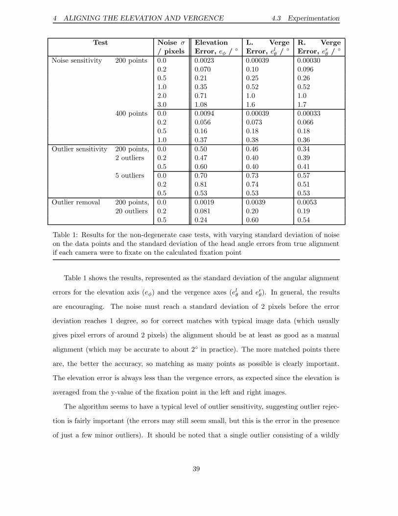
4 ALIGNING THE ELEVATION AND VERGENCE 4.3 Experimentation
Test Noise σ/ pixels
ElevationError, eφ / ◦
L. VergeError, el
θ / ◦
R. VergeError, er
θ / ◦
Noise sensitivity 200 points 0.0 0.0023 0.00039 0.000300.2 0.070 0.10 0.0960.5 0.21 0.25 0.261.0 0.35 0.52 0.522.0 0.71 1.0 1.03.0 1.08 1.6 1.7
400 points 0.0 0.0094 0.00039 0.000330.2 0.056 0.073 0.0660.5 0.16 0.18 0.181.0 0.37 0.38 0.36
Outlier sensitivity 200 points, 0.0 0.50 0.46 0.342 outliers 0.2 0.47 0.40 0.39
0.5 0.60 0.40 0.415 outliers 0.0 0.70 0.73 0.57
0.2 0.81 0.74 0.510.5 0.53 0.53 0.53
Outlier removal 200 points, 0.0 0.0019 0.0039 0.005320 outliers 0.2 0.081 0.20 0.19
0.5 0.24 0.60 0.54
Table 1: Results for the non-degenerate case tests, with varying standard deviation of noiseon the data points and the standard deviation of the head angle errors from true alignmentif each camera were to fixate on the calculated fixation point
Table 1 shows the results, represented as the standard deviation of the angular alignment
errors for the elevation axis (eφ) and the vergence axes (elθ and er
θ). In general, the results
are encouraging. The noise must reach a standard deviation of 2 pixels before the error
deviation reaches 1 degree, so for correct matches with typical image data (which usually
gives pixel errors of around 2 pixels) the alignment should be at least as good as a manual
alignment (which may be accurate to about 2◦ in practice). The more matched points there
are, the better the accuracy, so matching as many points as possible is clearly important.
The elevation error is always less than the vergence errors, as expected since the elevation is
averaged from the y-value of the fixation point in the left and right images.
The algorithm seems to have a typical level of outlier sensitivity, suggesting outlier rejec-
tion is fairly important (the errors may still seem small, but this is the error in the presence
of just a few minor outliers). It should be noted that a single outlier consisting of a wildly
39

4 ALIGNING THE ELEVATION AND VERGENCE 4.3 Experimentation
(a) Most depth. elθ = −0.6◦, e
rθ = 1.2◦, eφ = 1.6◦ (b) Mid. depth. e
lθ = 0.8◦, e
rθ = −1.9◦, eφ = 0.8◦
(c) Least depth. elθ = 1.7◦, e
rθ = −1.9◦, eφ = 0.2◦ (d) Bad start. e
lθ = −1.8◦, e
rθ = 0.4◦, eφ = 4.1◦
(e) Bad start. elθ = −2.3◦, e
rθ = 1.4◦, eφ = 5.0◦ (f) True alignment
Figure 12: The real image data used to test the non-degenerate case alignment
incorrect match (of the order of the size of the image) gave huge errors, but this kind of outlier
should never slip through the outlier rejection processes, so it is fair enough to test sensitivity
on matches that are incorrect by only 5 pixels. It is interesting to note that the error reduces
as noise increases, which illustrates, given that the noise ‘masks’ the outliers, the way in which
it is outliers, not noise, that dominate the accuracy of the algorithm (outliers with no noise
result in greater error than noise with no outliers). It also suggests something to be tested
– could noise artificially added to the data actually improve the performance for real data?
The outlier rejection tests illustrate the successful removal of the outliers and the return of
the error to its previous levels.
40
4 ALIGNING THE ELEVATION AND VERGENCE 4.3 Experimentation
Real data
The algorithm was tested on a variety of different scenes. At least 50% of the time, the
procedure fails to obtain enough matches at the stereo matching stage, and this runs through
to a poor result because the projective structure is bad and there are not enough matches to
overcome noise. This is a problem mainly with the disparity matcher, which provides a poor
initial match set for RANSAC, and the corner detector. This problem must be examined, but
for the moment is not relevant to testing of the algorithm itself. Figure 12 shows typical results
for scenes where more than 100 initial stereo matches were made, which is an approximate
minimum requirement. In the first three scenes there is the same (mildly off) initial alignment
with varying depth of structure. The other two scenes have poorer initial alignment. The
green lines show the position of the calculated lines at infinity (sometimes they are off the
image). The astute reader will note that the scenes have been somewhat fabricated to ensure
there are sufficient features.
To measure the alignment errors, a manual alignment was taken as the reference, so the
figures are not exactly accurate. Taking that into account, the method seems, at this stage, to
be overall a little worse than an alignment by eye. The algorithm did perform better overall
when there was most depth of structure in the scene (although it is not clear from these
specific scenes). Note that the elevation is usually better than the vergence, understandable
since it is taken from the average of the required elevation for the left and the right cameras.
The performance was considerably worse if the initial alignment was poor, although this
was largely due to the unguided fixation required when the fixation point does not lie on the
image. This could be handled by recalculating the fixation point if initially it is out of the
image (as was not done in these tests).
Conclusions
The combined evidence of the tests points to insufficient matches as the main cause of error.
Much of the problem lies with the disparity matcher, with insufficient matches leading to
an inadequate fundamental matrix calculation and so poor projective structure. This means
most of the matches are rejected in the 3D homography calculation. The problem may not
be so severe if the points themselves are adjusted at the minimisation stage to remove noise.
41
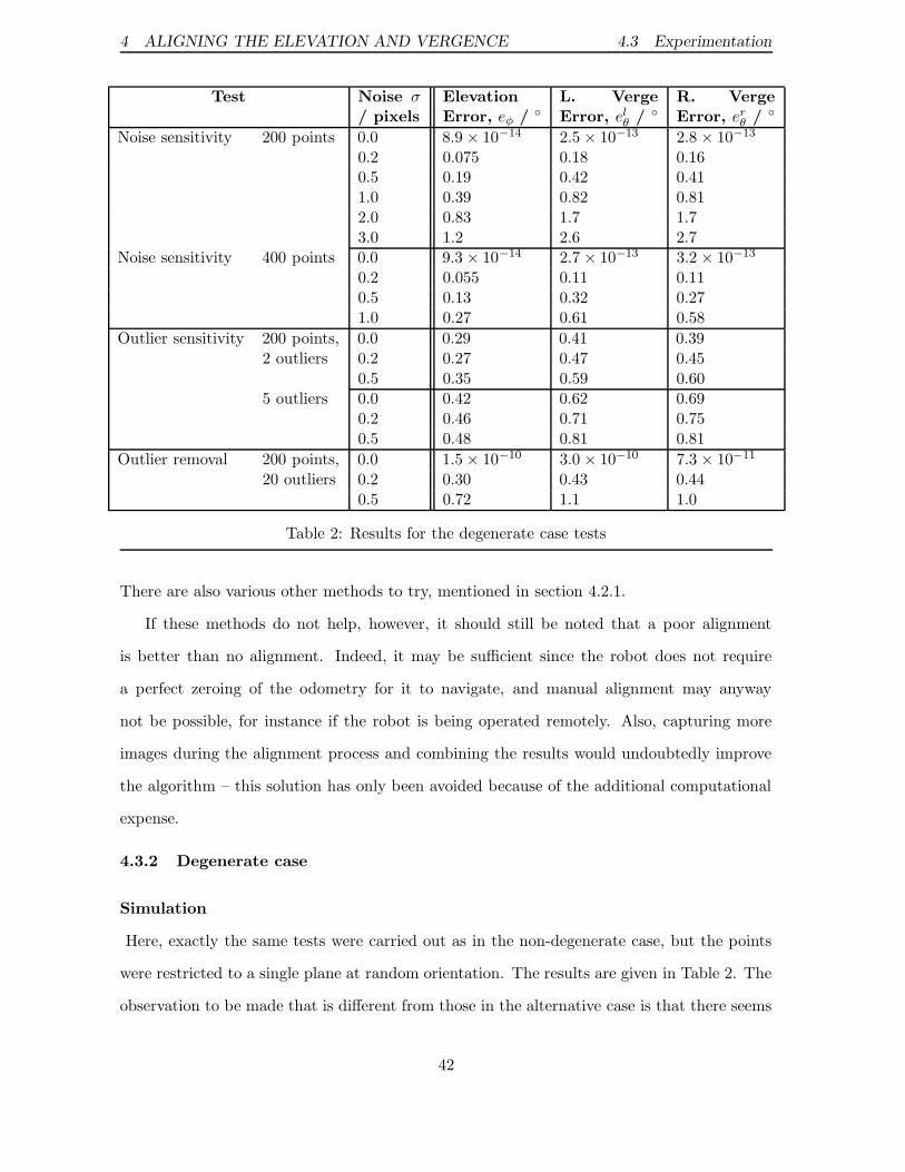
4 ALIGNING THE ELEVATION AND VERGENCE 4.3 Experimentation
Test Noise σ/ pixels
ElevationError, eφ / ◦
L. VergeError, el
θ / ◦
R. VergeError, er
θ / ◦
Noise sensitivity 200 points 0.0 8.9 × 10⁻¹⁴ 2.5 × 10⁻¹³ 2.8 × 10⁻¹³
0.2 0.075 0.18 0.160.5 0.19 0.42 0.411.0 0.39 0.82 0.812.0 0.83 1.7 1.73.0 1.2 2.6 2.7
Noise sensitivity 400 points 0.0 9.3 × 10⁻¹⁴ 2.7 × 10⁻¹³ 3.2 × 10⁻¹³
0.2 0.055 0.11 0.110.5 0.13 0.32 0.271.0 0.27 0.61 0.58
Outlier sensitivity 200 points, 0.0 0.29 0.41 0.392 outliers 0.2 0.27 0.47 0.45
0.5 0.35 0.59 0.605 outliers 0.0 0.42 0.62 0.69
0.2 0.46 0.71 0.750.5 0.48 0.81 0.81
Outlier removal 200 points, 0.0 1.5 × 10⁻¹⁰ 3.0 × 10⁻¹⁰ 7.3 × 10⁻¹¹
20 outliers 0.2 0.30 0.43 0.440.5 0.72 1.1 1.0
Table 2: Results for the degenerate case tests
There are also various other methods to try, mentioned in section 4.2.1.
If these methods do not help, however, it should still be noted that a poor alignment
is better than no alignment. Indeed, it may be sufficient since the robot does not require
a perfect zeroing of the odometry for it to navigate, and manual alignment may anyway
not be possible, for instance if the robot is being operated remotely. Also, capturing more
images during the alignment process and combining the results would undoubtedly improve
the algorithm – this solution has only been avoided because of the additional computational
expense.
4.3.2 Degenerate case
Simulation
Here, exactly the same tests were carried out as in the non-degenerate case, but the points
were restricted to a single plane at random orientation. The results are given in Table 2. The
observation to be made that is different from those in the alternative case is that there seems
42
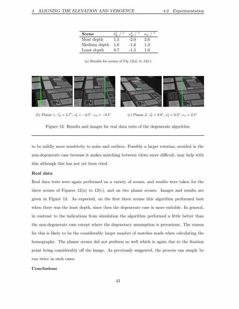
4 ALIGNING THE ELEVATION AND VERGENCE 4.3 Experimentation
Scene elθ / ◦ er
θ / ◦ eφ / ◦
Most depth 1.5 -2.0 2.6Medium depth 1.6 -1.6 1.3Least depth 0.7 -1.5 1.0
(a) Results for scenes of Fig 12(a) to 12(c)
(b) Planar 1. elθ = 4.7◦, e
rθ = −2.5◦, eφ = −0.5◦ (c) Planar 2. e
lθ = 8.8◦, e
rθ = 0.3◦, eφ = 2.4◦
Figure 13: Results and images for real data tests of the degenerate algorithm
to be mildly more sensitivity to noise and outliers. Possibly a larger rotation, avoided in the
non-degenerate case because it makes matching between views more difficult, may help with
this although this has not yet been tried.
Real data
Real data tests were again performed on a variety of scenes, and results were taken for the
three scenes of Figures 12(a) to 12(c), and on two planar scenes. Images and results are
given in Figure 13. As expected, on the first three scenes this algorithm performed best
when there was the least depth, since then the degenerate case is more suitable. In general,
in contrast to the indications from simulation the algorithm performed a little better than
the non-degenerate case except where the degeneracy assumption is precarious. The reason
for this is likely to be the considerably larger number of matches made when calculating the
homography. The planar scenes did not perform so well which is again due to the fixation
point being considerably off the image. As previously suggested, the process can simply be
run twice in such cases.
Conclusions
43
4 ALIGNING THE ELEVATION AND VERGENCE 4.3 Experimentation
The degenerate case does not suffer from lack of point matches as does the non-degenerate
case, because a homography calculation is more robust and accurate than a fundamental
matrix calculation, especially if the two images are genuinely related by a homography. Also,
if there is depth in the scene that invalidates that assumption, the robust procedure should
reject points that do not fit a homography, keeping only those points that are distant, or lie
on a single plane. This, combined with the reduced computational expense of this procedure
and its better performance, suggests that it should be used wherever possible; and it should
be possible in most practical situations, since for a typical stereo head the rotation axes are
close to the camera optical centres, so the rotation is near-degenerate. It is likely, however,
to have the disadvantage of less accurate self-calibration properties.
The procedure is still not quite as good as a manual alignment even when the initial
alignment is good. Possibly, larger rotations would help provide a more accurate homography,
as would forcing the homography into a form consistent with the type of motion involved.
4.3.3 Fixation
The fixation algorithm was used more as a tool for self-alignment than a research topic in
itself. It is suffices to say here that the algorithm worked well, usually achieving fixation
within three or four motions. It should be noted, however, that due to the simplifications of
§4.1.5, the algorithm cannot be used to obtain valid values for the focal lengths αlv etc.
4.3.4 Self-calibration
Experimentation for self-calibration is not covered by this report. In summary, the calibration
achieved is suitable for all but the most accurate visual measurement tasks. It is certainly
sufficient to aid rapid fixation in combination with image correlation.
44
5 ALIGNMENT WITH FORWARD DIRECTION
5 Alignment with Forward Direction
Aligning the head with the forward direction, ie. aligning the pan axis, is theoretically a trivial
problem. The cameras need to be fixated on the centre of expansion of optical flow in the
image as the robot moves forwards. This is, of course, the epipole. This report has already
covered how to calculate the epipole from two images. So simply calculate the fundamental
matrix representing the relationship between camera images before and after a forward motion
of the robot. Calculate the epipole using equation 9 and fixate.
It can take around 30 seconds to calculate the fundamental matrix, however, so this is
not a real time solution. Knowledge of the forward direction is a very useful navigational aid,
particularly because that is where obstacles in the robot’s path will be found. It is considered a
useful ability if the robot can calculate the forward direction in real time during its navigating
task, independently of the the head odometry, dead-reckoning, and map-building elements
which may be misleading. So interest turned to methods of locating the epipole that might
be done rapidly.
5.1 Theory
One possibility is the epipole estimation using affine motion parallax algorithm suggested by
Lawn and Cipolla [30]. This uses the disparity between points as the camera moves to locate
the epipole. It only uses a small number of point matches, but is slowed by the need to do the
matching. Since calculating the fundamental matrix would defeat the object, the matching
would need to use disparity, which may introduce outliers that invalidate the procedure.
First, therefore, a different method was considered. This used Brooks and Baumela’s
results for the differential epipolar equation [4, 5]. This is essentially the differential form of
the fundamental matrix equation. The derivation is long, so just the result is given here. For
each image pixel x with associated optical flow (velocity in the image) x, there is a relationship
x>Cx + x>Vx = 0 (17)
C and V are 3×3 matrices, the former encoding the camera rotation, and the latter the camera
translation. In fact, V is specifically an antisymmetric matrix which could be represented by
45
5 ALIGNMENT WITH FORWARD DIRECTION 5.1 Theory
vector v = [v1 v2 v3]>,
V =
0 −v3 v2
v3 0 −v1
−v2 v1 0
(18)
C is a symmetric matrix which could be represented by six parameters, c1 to c6. v, it turns out,
is the nonhomogeneous camera velocity in units of pixels (per frame). This is the trajectory
along which the camera centre is moving, and it pierces the image plane at v in homogeneous
pixel coordinates – so it represents the epipole.
Equation 17 can be rewritten:
[ x2 2xy 2x y2 2y 1 (y − y) (x − x) (yx − xy) ] π(C, V) = 0
⇒ m π(C, V) = 0
where x = [x y 1]> and x = [x y 1]>, and π(C, V) = [c1 c2 c3 c4 c5 c6 v1 v2 v3]>. So
9 or more m vectors can be stacked up to form a design matrix M, and the elements of C and
V can then be found by the DLT.
The only question that remains is how best to determine x.
5.1.1 Determining optical flow
Optical flow, the image motion of scene points associated with each pixel in an image, can only
be determined exactly using knowledge of the scene structure, camera motion and camera
matrices. However, it can be approximated easily and quickly by making a key assumption:
that any change in a pixel’s intensity over time is a result of translation of the local intensity
distribution. This assumption would be true if all surfaces were perfectly Lambertian, convex,
with no occlusions, and the lighting was uniformly ambient. Obviously this is never true, but
it does enable the derivation of some useful results.
The method adopted here is that propounded by Reid and North [38], derived from Lucas
and Kanade [32], which essentially tries to find the pixel in the second image whose local
distribution best matches that around the pixel of interest. For image point (x, y) with
intensity I(x, y, k) at frame k minimise
Ex(x, y) =∑
ij
(I(x + j + x, v + i + v, k + 1) − I(x, y, k))2
46

5 ALIGNMENT WITH FORWARD DIRECTION 5.2 Implementation
where the indices i, j range over a small patch. A first order approximation to the term in
brackets, and substitution of a gaussian convolution (represented by ⊗) for the sum leads to
the equation[
G ⊗ I2x G ⊗ IxIy
G ⊗ IxIy G ⊗ I2y
]
x +
[
G ⊗ IxIt
G ⊗ IyIt
]
= Mx + b = 0 (19)
where G is the gaussian kernel.
If x is at a point of uniform intensity, M will have rank zero since the distribution around
x will match equally well to all points in the area. If x lies on an edge it will match equally
well to all points along the edge, and M will have rank 1. In the first case flow cannot be
calculated, but in the second case the magnitude of flow perpendicular to the edge can still
be obtained. Here we choose to ignore all flow that is not fully determined.
5.2 Implementation
The implementation of this algorithm is rather simpler than for self-alignment of the elevation
and vergence. Note that, of course, this method could be used to align the elevation as well
as the vergence, although the alignment will be different – here it will be aligned parallel to
the floor rather than perpendicular to the pan axis. If the robot is built properly these should
be the same! Also, only one camera is used.
Start by setting off the robot moving slowly forwards. Grab images repeatedly from one
camera, and for each successive pair of images,
1. Calculate optic flow as in §5.1.1, retaining only fully determined flow vectors.
2. Use the flow vectors and their corresponding pixel locations to assemble matrix M and
calculate π(C, V) using the DLT.
3. Extract vector v from π(C, V).
4. Start the head turning towards fixation on v. In the case of Yorick (and most stereo
heads) the axis demands are controlled by a separate processor so the algorithm can
continue while the head is turning.
47
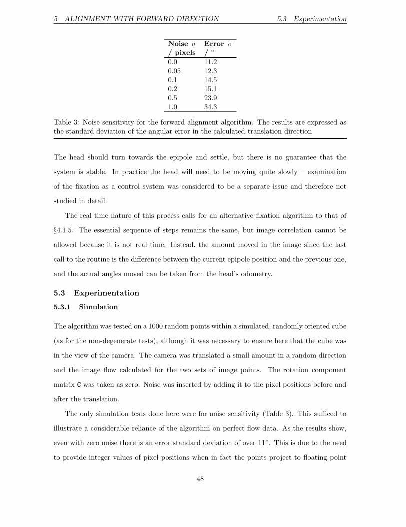
5 ALIGNMENT WITH FORWARD DIRECTION 5.3 Experimentation
Noise σ/ pixels
Error σ/ ◦
0.0 11.20.05 12.30.1 14.50.2 15.10.5 23.91.0 34.3
Table 3: Noise sensitivity for the forward alignment algorithm. The results are expressed asthe standard deviation of the angular error in the calculated translation direction
The head should turn towards the epipole and settle, but there is no guarantee that the
system is stable. In practice the head will need to be moving quite slowly – examination
of the fixation as a control system was considered to be a separate issue and therefore not
studied in detail.
The real time nature of this process calls for an alternative fixation algorithm to that of
§4.1.5. The essential sequence of steps remains the same, but image correlation cannot be
allowed because it is not real time. Instead, the amount moved in the image since the last
call to the routine is the difference between the current epipole position and the previous one,
and the actual angles moved can be taken from the head’s odometry.
5.3 Experimentation
5.3.1 Simulation
The algorithm was tested on a 1000 random points within a simulated, randomly oriented cube
(as for the non-degenerate tests), although it was necessary to ensure here that the cube was
in the view of the camera. The camera was translated a small amount in a random direction
and the image flow calculated for the two sets of image points. The rotation component
matrix C was taken as zero. Noise was inserted by adding it to the pixel positions before and
after the translation.
The only simulation tests done here were for noise sensitivity (Table 3). This sufficed to
illustrate a considerable reliance of the algorithm on perfect flow data. As the results show,
even with zero noise there is an error standard deviation of over 11◦. This is due to the need
to provide integer values of pixel positions when in fact the points project to floating point
48
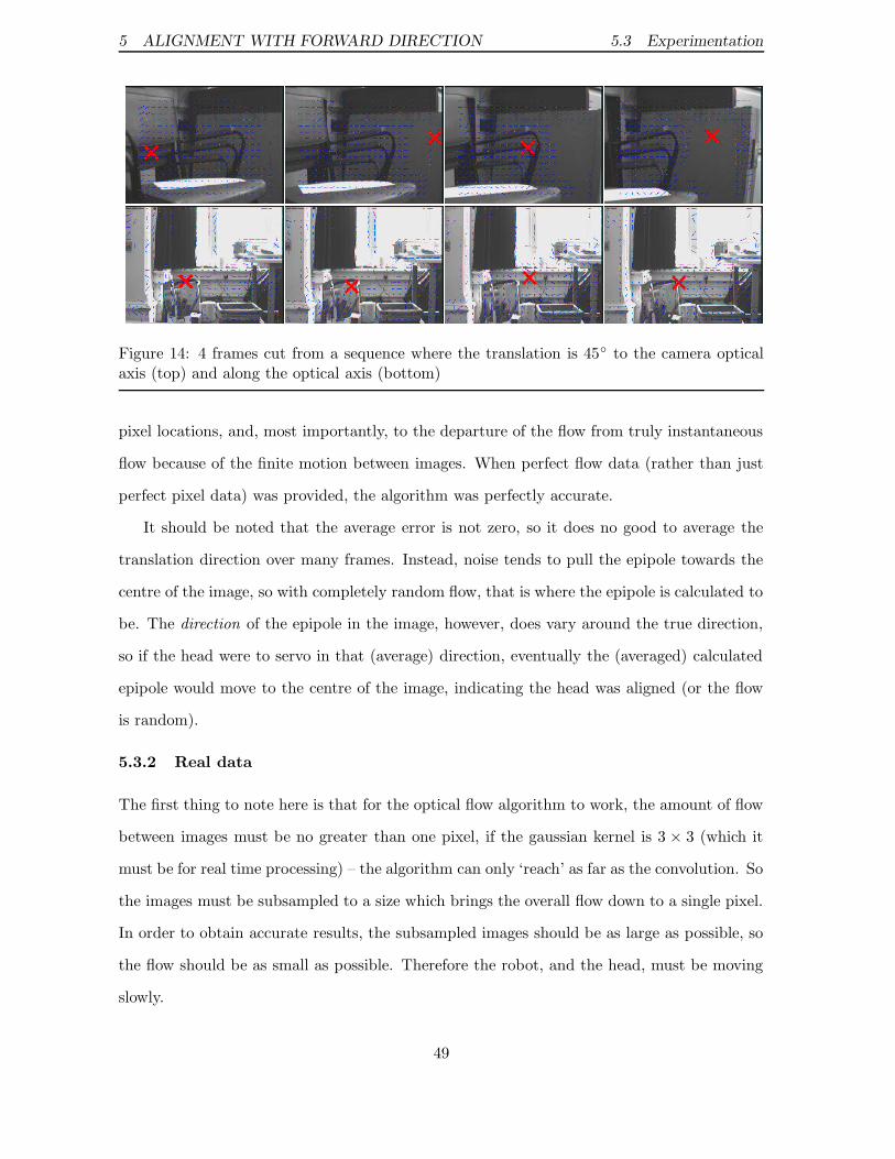
5 ALIGNMENT WITH FORWARD DIRECTION 5.3 Experimentation
Figure 14: 4 frames cut from a sequence where the translation is 45◦ to the camera opticalaxis (top) and along the optical axis (bottom)
pixel locations, and, most importantly, to the departure of the flow from truly instantaneous
flow because of the finite motion between images. When perfect flow data (rather than just
perfect pixel data) was provided, the algorithm was perfectly accurate.
It should be noted that the average error is not zero, so it does no good to average the
translation direction over many frames. Instead, noise tends to pull the epipole towards the
centre of the image, so with completely random flow, that is where the epipole is calculated to
be. The direction of the epipole in the image, however, does vary around the true direction,
so if the head were to servo in that (average) direction, eventually the (averaged) calculated
epipole would move to the centre of the image, indicating the head was aligned (or the flow
is random).
5.3.2 Real data
The first thing to note here is that for the optical flow algorithm to work, the amount of flow
between images must be no greater than one pixel, if the gaussian kernel is 3 × 3 (which it
must be for real time processing) – the algorithm can only ‘reach’ as far as the convolution. So
the images must be subsampled to a size which brings the overall flow down to a single pixel.
In order to obtain accurate results, the subsampled images should be as large as possible, so
the flow should be as small as possible. Therefore the robot, and the head, must be moving
slowly.
49
5 ALIGNMENT WITH FORWARD DIRECTION 5.3 Experimentation
The procedure was tested on two short image sequences taken from Yorick’s left camera
(Figure 14). In the first, a sequence of 12 frames, the camera was facing at approximately
45◦ to the robot’s motion. In the second, a sequence of 10 frames, the camera was facing
forwards. In both cases the vergence and elevation of the camera was already aligned. In the
images, the blue lines indicate the flow and the red cross or arrow indicates the calculated
position of the epipole. This clearly demonstrates the epipole position moving around the
image plane, never in the correct place. In the first sequence it is supposed to be off the image
to the right. In the second it is only close to the centre, where it should be, because the flow
is not particularly good.
Averaging the epipole position would have little meaning over these short sequences, so
quantitative results are not given here. The two sequences are sufficient to illustrate the
failure of the procedure. Note that in the first sequence the calculated flow seems to be quite
good, demonstrating the acute sensitivity of the procedure to noise. Nevertheless, the flow
calculation itself is the cause of much of the error, as illustrated by the second sequence.
5.3.3 Discussion
The epipole calculation has been carried out with no regard to the accuracy of the calculated
flow. Outlier rejection and smoothing have not been carried out because of the necessity
of keeping the procedure as fast as possible. However there is some scope for such robust
techniques in a real time context. For instance, a flow vector can be rejected if it varies too
greatly from its neighbours, a validity check that should incur negligible additional latency.
Should these techniques fail, however, it must be concluded that this method is not viable
for this application. Given the acute sensitivity of the procedure to noise, it seems most
likely that a robust fundamental matrix calculation using sparse feature points to reduce
computational expense is likely to be more successful for real time pan axis alignment.
50

A DECOMPOSING A 3D HOMOGRAPHY
A Decomposing a 3D homography
Any 4 × 4 homography H which is essentially a euclidean motion in projective space can be
decomposed as follows [27]:
H = αH−1
PED12HPE (20)
= α
[
K−1 0a> d
]
−1 [
R t0> 1
] [
K−1 0a> d
]
= α
[
KRK−1 + Kta> dKt1
d
(
−a>KRK−1 − a>Kta> + a>)
−a>Kt + 1
]
(21)
The following is a practical algorithm for decomposing any 4×4 matrix into this form, so that
the results can be used to initialise a minimisation routine to calculate H in the correct form
from a linear estimate. There are three stages, and progression to the next stage requires the
fulfillment of some criterium for H such that, for instance any singular matrix will fail at the
first stage. However, the algorithm ensures a decomposition is always provided which will
recompose into a matrix as close as possible to H (in some algebraic sense), the idea being
that should the decomposition fail to complete, the results can still be used to initialise a
minimisation routine.
1. First, find initial values for HPE and D12 that are obtainable for any 4 × 4 matrix H:
• Set M as the top left 3×3 sub-matrix of H, and take its singular value decomposition
(SVD) such that M = UΣV>. Now set the rotation R = UI3V>, where In is the n×n
identity matrix.
• Set α = norm(H), or 1 if norm(H) is zero, and put H = H/α. Set t equal to the top
right 3 × 1 sub-matrix of H. (Choice of norm is not crucial since this is only very
rough initialisation – the largest singular value is a good choice.)
• Set HPE = I4.
Obviously, this decomposition is not ideal.
2. If H is singular the algorithm ends here. Otherwise, remove the factor α. α is equal to
the single repeated real eigenvalue of H, and we know
51
A DECOMPOSING A 3D HOMOGRAPHY
α = 4
√
det(H)
Set H = H/α and divide up as follows:
H =
[
H hk> s
]
Now, the plane at infinity [a> d]> is equal to the eigenvector associated with the single
repeated real eigenvalue of H−> [49]. Since the eigenvalues of H−> are the same as those
of H, the plane at infinity is also equal to the eigenvector associated with the single
repeated real eigenvalue of 1 of H−>. This can be calculated with robustness to errors
by taking[
ad
]
= null(H−> − I4)
where here null(M) is the least-squares approximation to the right null-space of M, i.e.
the rightmost column of V from the SVD of M (M = UΣV>).
There is a scale ambiguity in the above calculation, and it is common procedure at this
stage to normalise [a> d]> such that d = 1. This makes no difference to the validity of
the decomposition.
3. Calculate the infinite homography,
H∞ = KRK−1 [49]
= H− Kta> (from equation 21)
= H−ha>
d
So we have
R = K−1H∞K (22)
and from the orthonormality of rotation matrices,
K>H−>
∞K−> = K−1H∞K
⇒ (KK>)H−>
∞= H∞(KK>) (23)
52
A DECOMPOSING A 3D HOMOGRAPHY
This is the equation arrived at by Hartley in his self-calibration papers [23, 24]. It gives
rise to a set of nine linear equations in the six independent entries of the symmetric
matrix C = KK>. These are not independent equations and a single H∞ is only sufficient
to solve for C to a 1 parameter family in addition to the inherent scale ambiguity. If the
purpose of this decomposition is to force H into the required form rather than actually
calculate the parameters K, R and t, then this is sufficient, otherwise the H∞ matrices
calculated from two independent H’s must be used together to solve for C. In either case
there is a simple linear (least-squares) solution.
If C (or −C, noting the scale-ambiguity) is not positive-definite, it is not possible to solve
for K and the decomposition ends here. Otherwise, procede with Cholesky factorisation
of C:
(a) Eigendecompose C, so C = UDU>
(b) D is diagonal. Take its square root, D = EE>. Thus C = UEE>U>.
(c) QR-decompose (UE)−1, so (UE)−1 = QK−1 where Q is orthogonal and K−1 is upper
triangular. So C = KQ>QK> = KK> as required.
Normalise K so that its (3, 3) element is 1. Finally, solve for R from (22), and for t from
(21) thus:
t = K−1h
d
It is only possible to solve for t up to an unknown scale factor (so it is all right to leave
d out of the above equation). This gives G and D12.
53
B SUMMARY OF NOTATION AND EQUATIONS
B Summary of Notation and Equations
B.1 Notation
x Lower case bold; 3-vector, 2D homogeneous vector
X Upper case bold; 4-vector, 3D homogeneous vector
M Upper case teletype; Matrix
I Identity matrix, size from context
In n × n identity matrix
R 3 × 3 rotation matrix
t 3 × 1 non-homogeneous translation vector
λ,Π Line in 2D, plane in 3D
Π∞, Π∞P Plane at infinity in euclidean space, in projective space
X = (X,Y,Z) World coordinates
Xc = (Xc, Yc, Zc) Camera-centred coordinates
xi Image plane coordinates (metric)
x Pixel coordinates
[u0 v0 1]> Principal point in pixel coordinates
αu, αv Focal lengths in x-pixels and y-pixels
K Calibration matrix
P, PP Calibrated camera (projection) matrix, projective camera matrix
H, H2D General 3D (4 × 4) homography, general 2D homography
HPE Update matrix, from projective to euclidean space
C, e, l Camera centre, epipole, epipolar line
C′, e′, l′ Prime (′) indicates other view
F Fundamental matrix
D Generalised euclidean transformation of 3-space
XE, X′
E, XP, X′
PPoints in original and rotated 3-space, euclidean and projective
[a> d]> Plane at infinity in projective space
V, V3, V4 Eigenvector of H, the complex ones
λ1 . . . λ4 Eigenvalues of H
θ, φ Vergence, elevation
PP
l, PP
r Superscripts l and r indicate left and right images
C, V Rotation and velocity parts of optic flow respectively
π(C, V) Independent elements of C and V as a vector
elθ, er
θ, eφ Left and right vergence, and elevation errors
54
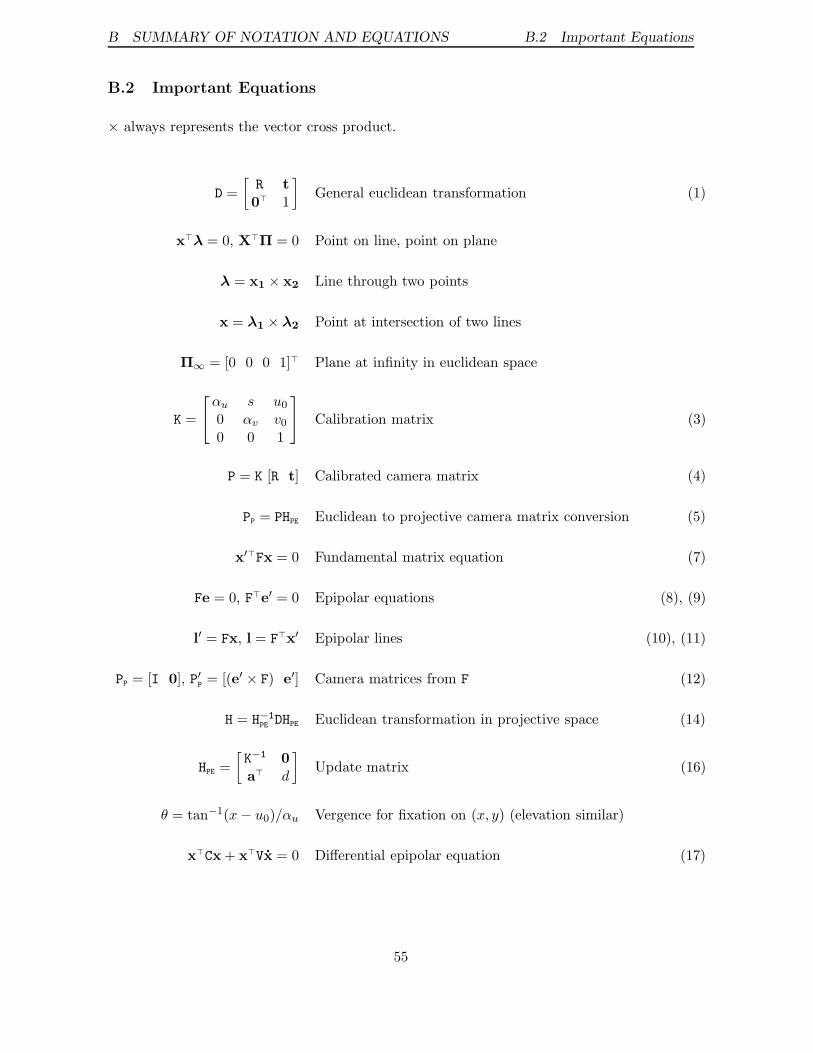
B SUMMARY OF NOTATION AND EQUATIONS B.2 Important Equations
B.2 Important Equations
× always represents the vector cross product.
D =
[
R t0> 1
]
General euclidean transformation (1)
x>λ = 0, X>Π = 0 Point on line, point on plane
λ = x1 × x2 Line through two points
x = λ1 × λ2 Point at intersection of two lines
Π∞ = [0 0 0 1]> Plane at infinity in euclidean space
K =
αu s u0
0 αv v0
0 0 1
Calibration matrix (3)
P = K [R t] Calibrated camera matrix (4)
PP = PHPE Euclidean to projective camera matrix conversion (5)
x′>Fx = 0 Fundamental matrix equation (7)
Fe = 0, F>e′ = 0 Epipolar equations (8), (9)
l′ = Fx, l = F>x′ Epipolar lines (10), (11)
PP = [I 0], P′P= [(e′ × F) e′] Camera matrices from F (12)
H = H−1
PEDHPE Euclidean transformation in projective space (14)
HPE =
[
K−1 0a> d
]
Update matrix (16)
θ = tan−1(x − u0)/αu Vergence for fixation on (x, y) (elevation similar)
x>Cx + x>Vx = 0 Differential epipolar equation (17)
55
REFERENCES REFERENCES
References
[1] P. A. Beardsley, I. D. Reid, A. Zisserman, and D. W. Murray. Active visual navigationusing non-metric structure. In Proc. 5th Int’l Conf. on Computer Vision, Cambridge,MA, pages 58–64. IEEE Computer Society Press, June 1995.
[2] P. A. Beardsley, A. Zisserman, and D. W. Murray. Sequential updating of projective andaffine structure from motion. International Journal of Computer Vision, 23(3):235–259,June 1997.
[3] Paul A. Beardsley and Andrew Zisserman. Affine calibration of mobile vehicles. InR. Mohr and W. Chengke, editors, Proc. Joint Europe-China Workshop on GeometricalModelling and Invariants for Computer Vision, Xi’an, China. Xi’an University Press,1995.
[4] Michael J. Brooks, Luis Baumela, and Wojciech Chojnacki. An analytical approachto determining the ego-motion of a camera having free intrinsic parameters. TechnicalReport TR96-04, Department of Computer Science, University of Adelaide, June 1996.
[5] Michael J. Brooks, Wojniech Chojnacki, and Luis Baumela. Determining the egomotionof an uncalibrated camera from instantaneous optical flow. Journal of the Optical Societyof America, 14(10), October 1997.
[6] T. P. H. Burke. Design of a Modular Mobile Robot. PhD thesis, University of OxfordDepartment of Engineering Science, 1994.
[7] Francois Chaumette, Ezio Malis, and Sylvie Boudet. 2 1
2d visual servoing with respect
to planar objects. In Proc. IEEE/RSJ Int’l Conf. on Intelligent Robots and Systems,Workshop on New Trends in Image-Based Servoing, Grenoble, France, pages 45–52,September 1997.
[8] A. Criminisi, I. Reid, and A. Zisserman. Single view metrology. In Proc. 6th Int’l Conf.on Computer Vision, Bombay, 1999.
[9] Andrew Davison. Mobile Robot Navigation Using Active Vision. PhD thesis, RoboticsResearch Group, Oxford University Department of Engineering Science, February 1998.Available from www.robots.ox.ac.uk/~ajd/.
[10] Andrew J. Davison and David W. Murray. Mobile robot localisation using active vision.In Proc. 5th European Conf. on Computer Vision, Freiburg, number 1407 in LectureNotes in Computer Science, pages 809–825. Springer-Verlag, 1998.
[11] L. de Agapito, E. Hayman, and I. Reid. Self-calibration of a rotating camera withvarying intrinsic parameters. In Paul H. Lewis and Mark S. Nixon, editors, Proc. 9thBritish Machine Vision Conf., Southampton, volume 1, pages 105–114. BMVA Press,1998.
[12] Frederic Devernay and Olivier Faugeras. From projective to Euclidean reconstruction. InProc. IEEE Conf. on Computer Vision and Pattern Recognition, San Francisco, pages264–269. IEEE Computer Society Press, June 1996.
[13] Stuart M. Fairley, Ian D. Reid, and David W. Murray. Transfer of fixation for an activestereo platform via affine structure recovery. In Proc. 5th Int’l Conf. on Computer Vision,Cambridge, MA, pages 1100–1105. IEEE Computer Society Press, June 1995.
[14] Stuart M. Fairley, Ian D. Reid, and David W. Murray. Transfer of fixation using affinestructure: Extending the analysis to stereo. International Journal of Computer Vision,29(1):47–58, 1998.
56
REFERENCES REFERENCES
[15] O. D. Faugeras, Q.-T. Luong, and S. J. Maybank. Camera self-calibration: Theoryand experiments. In G. Sandini, editor, Proc. 2nd European Conf. on Computer Vision,Santa Margharita Ligure, Italy, number 588 in Lecture Notes in Computer Science, pages321–334. Springer-Verlag, May 1992.
[16] A. W. Fitzgibbon and A. Zisserman. Automatic 3D model acquisition and generationof new images from video sequences. In Proc. European Signal Processing Conference(EUSIPCO), Rhodes, Greece, pages 1261–1269, September 1998.
[17] J. J. Guerrero and C. Sagues. Navigation from uncalibrated monocular vision. In Proc.3rd IFAC Symposium on Intelligent Autonomous Vehicles, pages 210–215, 1998.
[18] Gregory D. Hager and Zachary Dodds. A projective framework for constructing accuratehand-eye systems. In Workshop on New Trends in Image-Based Servoing, IROS, pages71–82, 1997.
[19] C. G. Harris and M. Stephens. A combined corner and edge detector. In Proc. 4th AlveyVision Conf., Manchester, pages 147–151, 1988.
[20] R. I. Hartley and P. Sturm. Triangulation. In Proc. Conf. on Computer Analysis ofImages and Patterns, Prague, Czech Republic, 1995.
[21] R. I. Hartley and A. Zisserman. Multiple View Geometry in Computer Vision. CambridgeUniversity Press, 2000.
[22] Richard I. Hartley. Projective reconstruction from line correspondences. In Proc. IEEEConf. on Computer Vision and Pattern Recognition, pages 903–907, 1994.
[23] Richard I. Hartley. Euclidean reconstruction from uncalibrated views. In J. L. Mundy,A. Zisserman, and D. Forsyth, editors, Applications of Invariance in Computer Vision.The MIT Press, 1995.
[24] Richard I. Hartley. Self-calibration of stationary cameras. International Journal ofComputer Vision, 22(1):5–23, February 1997.
[25] Anders Heyden and Kalle Astrom. Euclidean reconstruction from constant intrinsicparameters. In Proc. 13th IEEE Int’l Conf. on Pattern Recognition, Vienna, pages 339–343. IEEE Computer Society Press, 1996.
[26] Anders Heyden and Kalle Astrom. Euclidean reconstruction from image sequences withvarying and unknown focal length and principal point. In Proc. IEEE Conf. on ComputerVision and Pattern Recognition, San Juan, Puerto Rico, pages 438–443. IEEE ComputerSociety Press, June 1997.
[27] Radu Horaud and Gabriella Csurka. Self-calibration and euclidean reconstruction usingmotions of a stereo rig. In Proc. 6th Int’l Conf. on Computer Vision, Bombay, pages96–103. IEEE Computer Society Press, January 1998.
[28] Huosheng Hu, Michael Brady, and Penelope Probert. Navigation and control of a mobilerobot among moving obstacles. In IEEE Conference on Decision and Control, 30, pages698–703, 1991.
[29] Takeo Kanade and Daniel D. Morris. Factorization methods for structure from motion.Philosophical Transactions of the Royal Society of London Series A, 356(1704):1153–1171, 1998.
[30] J. M. Lawn and R. Cipolla. Epipolar estimation using affine motion-parallax. In Proc.4th British Machine Vision Conf., Guildford, 1993.
[31] John J. Leonard and Hans Jacob S. Feder. Decoupled stochastic mapping. TechnicalMemorandum 99-1, MIT Marine Robotics Laboratory, December 1999.
57
REFERENCES REFERENCES
[32] B. D. Lucas and T. Kanade. Optical navigation by the method of differences. In Inter-national Joint Conference on Artificial Intelligence, volume 2 of 9, pages 981–984, LosAngeles, CA, August 1985. Morgan Kaufmann.
[33] Philip F. McLauchlan and David W. Murray. Active camera calibration for a head-eye platform using the variable state-dimension filter. IEEE Transactions on PatternAnalysis and Machine Intelligence, 18(1):15–21, January 1996.
[34] Joseph L. Mundy and Andrew Zisserman, editors. Geometric Invariance in ComputerVision, chapter 23, Appendix – Projective Geometry for Machine Vision, pages 463–519.MIT Press, 1992.
[35] D. W. Murray, I. D. Reid, and A. J. Davison. Steering and navigation behaviours usingfixation. In Proc. 7th British Machine Vision Conf., Edinburgh, pages 635–644. BMVAPress, 1996.
[36] D. W. Murray, I. D. Reid, and A. J. Davison. Steering without representation usingactive fixation. Perception, 26(12):1519–1528, 1997.
[37] N. E. Pears and J. R. Bumby. The steering control of an experimental autonomousvehicle. Trans. Institute of Measures and Control, 13(4):190–201, 1991.
[38] I. Reid and A. North. 3d trajectories from a single viewpoint using shadows. In Proc.9th British Machine Vision Conf., Southampton, 1998.
[39] I. D. Reid and P. A. Beardsley. Self-alignment of a binocular head. Image and VisionComputing, 14(8):635–640, August 1996.
[40] I. D. Reid and D. W. Murray. Active tracking of foveated feature clusters using affinestructure. International Journal of Computer Vision, 18(1):41–60, April 1996.
[41] Rolf Schuster, Nirwan Ansari, and Ali Bani-Hashemi. Steering a robot with vanishingpoints. In IEEE Transactions on Robotics and Automation, 9(4):491–498, 1993.
[42] J. G. Semple and G. T. Kneebone. Algebraic Projective Geometry. Oxford UniversityPress, 1952.
[43] P. M. Sharkey, D. W. Murray, S. Vandevelde, I. D. Reid, and P. F. McLauchlan. Amodular head/eye platform for real-time reactive vision. Mechatronics, 3(4):517–535,1993.
[44] Carlo Tomasi and Takeo Kanade. Shape and motion from image streams under orthog-raphy. International Journal of Computer Vision, 9(2):137–154, 1992.
[45] P. H. S. Torr and D. W. Murray. The development and comparison of robust meth-ods for estimating the fundamental matrix. International Journal of Computer Vision,24(3):271–300, September 1997.
[46] Phil Torr, Andrew W. Fitzgibbon, and Andrew Zisserman. Maintaining multiple modelhypotheses over many views to recover matching and structure. In Proc. 6th Int’l Conf.on Computer Vision, Bombay, pages 485–491. IEEE Computer Society Press, January1998.
[47] Bill Triggs. Autocalibration from planar scenes. In Proc. 5th European Conf.on Computer Vision, Freiburg, number 1406 in Lecture Notes in Computer Sci-ence, pages I:89–105. Springer-Verlag, June 1998. Extended version available athttp://www.inrialpes.fr/movi/people/Triggs/publications.html.
[48] Andrew Zisserman. Graduate computer vision series lecture notes. Oxford UniversityDepartment of Engineering Science internal, 1997.
58

REFERENCES REFERENCES
[49] Andrew Zisserman, Paul A. Beardsley, and Ian D. Reid. Metric calibration of a stereorig. In Proc. IEEE Workshop on Representations of Visual Scenes, in conjunction withICCV’95, Cambridge, MA, pages 93–100. IEEE Computer Society Press, June 1995.
59


![Lecture 8 Active stereo& - Stanford UniversitySilvio Savarese Lecture 7 - 12-Feb-18 Lecture 8 Active stereo& Volumetric stereo Reading: [Szelisky] Chapter 11 “Multi-view stereo”](https://img.pdfslide.us/doc/110x75/5f0f7f2f7e708231d444745e/lecture-8-active-stereo-stanford-university-silvio-savarese-lecture-7-12-feb-18.jpg)