Embed Size (px)
Citation preview
R–lab
Bernd Klaus1
European Molecular Biology Laboratory (EMBL),Heidelberg, Germany
April 30, 2015
Contents
1 Required packages and other preparations 1
2 Introduction and getting help 1
3 Basics – objects and arithmetic 2
4 Summaries, subscripting and useful vector functions 5
5 Classes, modes and types of objects 6
6 Matrices, lists, data frames and basic data handling 76.1 Matrices . . . . . . . . . . . . . . . . . . . . . . . . . . . . . . . . . . . . . . . . . . . . . . . . . . . . 76.2 Data frames and lists . . . . . . . . . . . . . . . . . . . . . . . . . . . . . . . . . . . . . . . . . . . . . 96.3 Apply functions . . . . . . . . . . . . . . . . . . . . . . . . . . . . . . . . . . . . . . . . . . . . . . . . 12
7 Plotting in R 137.1 Plotting in base R . . . . . . . . . . . . . . . . . . . . . . . . . . . . . . . . . . . . . . . . . . . . . . . 137.2 ggplot2 and qplot . . . . . . . . . . . . . . . . . . . . . . . . . . . . . . . . . . . . . . . . . . . . . . . 14
8 Calling functions and programming 198.1 Calling functions . . . . . . . . . . . . . . . . . . . . . . . . . . . . . . . . . . . . . . . . . . . . . . . . 198.2 Creating your own functions . . . . . . . . . . . . . . . . . . . . . . . . . . . . . . . . . . . . . . . . . 198.3 Flow control . . . . . . . . . . . . . . . . . . . . . . . . . . . . . . . . . . . . . . . . . . . . . . . . . . 20
9 Answers to exercises 21
1 Required packages and other preparations
library(TeachingDemos)
library(xlsx)
library(multtest)
library(Biobase)
library(plyr)
library(dplyr)
library(ggplot2)
1
R–lab 2
2 Introduction and getting help
R is a software language for carrying out complicated (and simple) statistical analyses. It includes routines for datasummary and exploration, graphical presentation and data modeling. The aim of this lab is to provide you with a basicfluency in the language. When you work in R you create objects that are stored in the current workspace (sometimescalled image). Each object created remains in the image unless you explicitly delete it. At the end of the session theworkspace will be lost unless you save it.
You can get your current working directory via getwd() and set it with setwd(). By default, it is usually your homedirectory.
Commands written in R are saved in memory throughout the session. You can scroll back to previous commands typedby using the “up” arrow key (and “down” to scroll back again). You finish an R session by typing q() at which pointyou will also be prompted as to whether or not you want to save the current workspace into your working directory. Ifyou do not want to, it will be lost. Remember the ways to get help:
• Just ask!• help.start() and the HTML help button in the Windows GUI.• help and ?: help("data.frame") or ?help.• help.search(), apropos()• browseVignettes("package")
• rseek.org• use tab–completion in RStudio, this will also display help–snippets
3 Basics – objects and arithmetic
R stores information in objects and operates on objects. The simplest objects are scalars, vectors and matrices. Butthere are many others: lists and data frames for example. In advanced use of R it can also be useful to define new typesof objects, specific for particular application. We will stick with just the most commonly used objects here. An importantfeature of R is that it will do different things on different types of objects. For example, type:
4 + 6
#> [1] 10
So, R does scalar arithmetic returning the scalar value 10. In fact, R returns a vector of length 1 - hence the [1] denotingfirst element of the vector. We can assign objects values for subsequent use. For example:
x <- 6
y <- 4
z <- x+y
z
#> [1] 10
would do the same calculation as above, storing the result in an object called z. We can look at the contents of theobject by simply typing its name. At any time we can list the objects which we have created:
ls()
#> [1] "x" "y" "z"
Notice that ls is actually an object itself. Typing ls would result in a display of the contents of this object, in this case,the commands of the function. The use of parentheses, ls(), ensures that the function is executed and its result — inthis case, a list of the objects in the current environment — displayed. More commonly, a function will operate on anobject, for example

R–lab 3
sqrt(16)
#> [1] 4
calculates the square root of 16. Objects can be removed from the current workspace with the function rm(). Thereare many standard functions available in R, and it is also possible to create new ones. Vectors can be created in R in anumber of ways. We can describe all of the elements:
z <- c(5,9,1,0)
Note the use of the function c to concatenate or “glue together” individual elements. This function can be used muchmore widely, for example
x <- c(5,9)
y <- c(1,0)
z <- c(x,y)
would lead to the same result by gluing together two vectors to create a single vector. Sequences can be generated asfollows:
seq(1,9,by=2)
#> [1] 1 3 5 7 9
seq(8,20,length=6)
#> [1] 8.0 10.4 12.8 15.2 17.6 20.0
These examples illustrate that many functions in R have optional arguments, in this case, either the step length or thetotal length of the sequence (it doesn’t make sense to use both). If you leave out both of these options, R will make itsown default choice, in this case assuming a step length of 1. So, for example,
x <- seq(1,10)
also generates a vector of integers from 1 to 10. At this point it’s worth mentioning the help facility again. If you don’tknow how to use a function, or don’t know what the options or default values are, type help(functionname) or simply?functionname where functionname is the name of the function you are interested in. This will usually help and willoften include examples to make things even clearer. Another useful function for building vectors is the rep command forrepeating things. Examples:
rep(1:3,6)
#> [1] 1 2 3 1 2 3 1 2 3 1 2 3 1 2 3 1 2 3
## repeat each element six times
rep(1:3,c(6,6,6))
#> [1] 1 1 1 1 1 1 2 2 2 2 2 2 3 3 3 3 3 3
## simplified
rep(1:3,rep(6,3))
#> [1] 1 1 1 1 1 1 2 2 2 2 2 2 3 3 3 3 3 3
As explained above, R will often adapt to the objects it is asked to work on. An example is the vectorized arithmeticused in R:
x <- 1:5; y <- 5:1
x
#> [1] 1 2 3 4 5
y
R–lab 4
#> [1] 5 4 3 2 1
x + y
#> [1] 6 6 6 6 6
x^2
#> [1] 1 4 9 16 25
# another example
x <- c(6,8,9)
y <- c(1,2,4)
x + y
#> [1] 7 10 13
x * y
#> [1] 6 16 36
showing that R uses component-wise arithmetic on vectors. R will also try to make sense if objects are mixed. Forexample,
x <- c(6,8,9)
x + 2
#> [1] 8 10 11
Two particularly useful functions worth remembering are length which returns the length of a vector (i.e. the numberof elements it contains) and sum which calculates the sum of the elements of a vector. R also has basic calculatorcapabilities:
• a+b, a-b, a∗b, a ˆ b (or a**b), a %% b (a MOD b)
• additionally: sqrt(a), sin(a) ...• and some simple statistics:
– mean(a)
– summary(a)
– var(a)
– min(a,b), max(a,b)
Exercise: Simple R operations
(a) Define x <- c(4,2,6) and y <- c(1,0,-1) Decide what the result will be of the following:(a) length(x)
(b) sum(x)
(c) sum(x^2)
(d) x+y
(e) x*y
(f ) x-2
(g) x^2
Use R to check your answers.(b) Decide what the following sequences are and use R to check your answers:
(a) 7:11
(b) seq(2,9)
(c) seq(4,10,by=2)
(d) seq(3,30,length=10)
(e) seq(6,-4,by=-2)
(c) Determine what the result will be of the following R expressions, and then use R to check you are right:(a) rep(2,4)
R–lab 5
(b) rep(c(1,2),4)
(c) rep(c(1,2),c(4,4))
(d) rep(1:4,4)
(e) rep(1:4,rep(3,4))
(d) Use the rep function to define simply the following vectors in R.(a) 6,6,6,6,6,6
(b) 5,8,5,8,5,8,5,8
(c) 5,5,5,5,8,8,8,8
Exercise: R as a calculator
Calculate the following expression, where x and y have values -0.25 and 2 respectively. Then store the result in a newvariable and print its content.
x + cos(pi/y)
4 Summaries, subscripting and useful vector functions
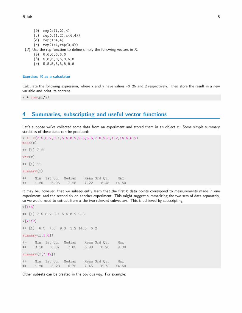
Let’s suppose we’ve collected some data from an experiment and stored them in an object x. Some simple summarystatistics of these data can be produced:
x <- c(7.5,8.2,3.1,5.6,8.2,9.3,6.5,7.0,9.3,1.2,14.5,6.2)
mean(x)
#> [1] 7.22
var(x)
#> [1] 11
summary(x)
#> Min. 1st Qu. Median Mean 3rd Qu. Max.
#> 1.20 6.05 7.25 7.22 8.48 14.50
It may be, however, that we subsequently learn that the first 6 data points correspond to measurements made in oneexperiment, and the second six on another experiment. This might suggest summarizing the two sets of data separately,so we would need to extract from x the two relevant subvectors. This is achieved by subscripting:
x[1:6]
#> [1] 7.5 8.2 3.1 5.6 8.2 9.3
x[7:12]
#> [1] 6.5 7.0 9.3 1.2 14.5 6.2
summary(x[1:6])
#> Min. 1st Qu. Median Mean 3rd Qu. Max.
#> 3.10 6.07 7.85 6.98 8.20 9.30
summary(x[7:12])
#> Min. 1st Qu. Median Mean 3rd Qu. Max.
#> 1.20 6.28 6.75 7.45 8.73 14.50
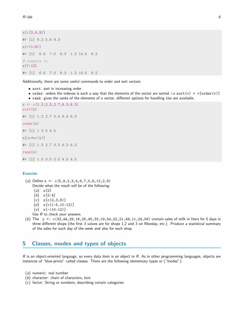
Other subsets can be created in the obvious way. For example:
R–lab 6
x[c(2,4,9)]
#> [1] 8.2 5.6 9.3
x[-(1:6)]
#> [1] 6.5 7.0 9.3 1.2 14.5 6.2
# compare to
x[7:12]
#> [1] 6.5 7.0 9.3 1.2 14.5 6.2
Additionally, there are some useful commands to order and sort vectors
• sort: sort in increasing order• order: orders the indexes is such a way that the elements of the vector are sorted, i.e sort(v) = v[order(v)]
• rank: gives the ranks of the elements of a vector, different options for handling ties are available.
x <- c(1.3,3.5,2.7,6.3,6.3)
sort(x)
#> [1] 1.3 2.7 3.5 6.3 6.3
order(x)
#> [1] 1 3 2 4 5
x[order(x)]
#> [1] 1.3 2.7 3.5 6.3 6.3
rank(x)
#> [1] 1.0 3.0 2.0 4.5 4.5
Exercise
(a) Define x <- c(5,9,2,3,4,6,7,0,8,12,2,9)
Decide what the result will be of the following:(a) x[2]
(b) x[2:4]
(c) x[c(2,3,6)]
(d) x[c(1:5,10:12)]
(e) x[-(10:12)]
Use R to check your answers.(b) The y <- c(33,44,29,16,25,45,33,19,54,22,21,49,11,24,56) contain sales of milk in liters for 5 days in
three different shops (the first 3 values are for shops 1,2 and 3 on Monday, etc.). Produce a statistical summaryof the sales for each day of the week and also for each shop.
5 Classes, modes and types of objects
R is an object-oriented language, so every data item is an object in R. As in other programming languages, objects areinstances of “blue-prints” called classes. There are the following elementary types or (“modes”):
(a) numeric: real number(b) character: chain of characters, text(c) factor: String or numbers, describing certain categories

R–lab 7
(d) logical: TRUE, FALSE(e) special values: NA (missing value), NULL (“empty object”), Inf, -Inf (infinity), NaN (not a number)
Data storage types includes matrices, lists and data frames, which will be introduced in the next section. Certain typescan have different subtypes, e.g. numeric can be further subdivided into the integer, single and double types. Types canbe checked by the is.* and changed (“casted”) by the as.* functions. Furthermore, the function str is very useful inorder to obtain an overview of an (possibly complex) object at hand. The following examples will make this clear:
#assign value "9" to an object
a <- 9
# is a a string?
is.character(a)
#> [1] FALSE
# is a a number?
is.numeric(a)
#> [1] TRUE
# What's its type?
typeof(a)
#> [1] "double"
# now turn it into a factor
a <- as.factor(a)
# Is it a factor?
is.factor(a)
#> [1] TRUE
# assign an string to a:
a <- "NAME"
# what's a?
class(a)
#> [1] "character"
str(a)
#> chr "NAME"
6 Matrices, lists, data frames and basic data handling
6.1 Matrices
Matrices can be created in R in a variety of ways. Perhaps the simplest is to create the columns and then glue themtogether with the command cbind. For example,
x <- c(5,7,9)
y <- c(6,3,4)
z <- cbind(x,y)
z
#> x y
#> [1,] 5 6
#> [2,] 7 3
#> [3,] 9 4

R–lab 8
## dimensions: 3 rows and 2 columns
dim(z)
#> [1] 3 2
### matrix constructor
z <- matrix(c(5,7,9,6,3,4),nrow=3)
There is a similar command, rbind, for building matrices by gluing rows together. The functions cbind and rbind canalso be applied to matrices themselves (provided the dimensions match) to form larger matrices. Matrices can also bebuilt by explicit construction via the function matrix. Notice that the dimension of the matrix is determined by the size ofthe vector and the requirement that the number of rows is 3 in the example above, as specified by the argument nrow=3.As an alternative we could have specified the number of columns with the argument ncol=2 (obviously, it is unnecessaryto give both). Notice that the matrix is “filled up” column-wise. If instead you wish to fill up row-wise, add the optionbyrow=T. For example:
z <- matrix(c(5,7,9,6,3,4),nr=3,byrow=T)
z
#> [,1] [,2]
#> [1,] 5 7
#> [2,] 9 6
#> [3,] 3 4
Notice that the argument nrow has been abbreviated to nr. Such abbreviations are always possible for function argumentsprovided it induces no ambiguity – if in doubt always use the full argument name. As usual, R will try to interpretoperations on matrices in a natural way. For example, with z as above, and
y <- matrix(c(1,3,0,9,5,-1),nrow=3,byrow=T)
y
#> [,1] [,2]
#> [1,] 1 3
#> [2,] 0 9
#> [3,] 5 -1
y + z
#> [,1] [,2]
#> [1,] 6 10
#> [2,] 9 15
#> [3,] 8 3
y * z
#> [,1] [,2]
#> [1,] 5 21
#> [2,] 0 54
#> [3,] 15 -4
Notice that multiplication here is component–wise rather than conventional matrix multiplication. Indeed, conventionalmatrix multiplication is undefined for y and z as the dimensions fail to match. Actual matrix multiplication works likethis:
x <- matrix(c(3,4,-2,6),nrow=2,byrow=T)
x
#> [,1] [,2]
#> [1,] 3 4
#> [2,] -2 6

R–lab 9
y %*% x
#> [,1] [,2]
#> [1,] -3 22
#> [2,] -18 54
#> [3,] 17 14
Other useful functions on matrices are t to calculate a matrix transpose and solve to calculate inverses:
t(z)
#> [,1] [,2] [,3]
#> [1,] 5 9 3
#> [2,] 7 6 4
solve(x)
#> [,1] [,2]
#> [1,] 0.2308 -0.154
#> [2,] 0.0769 0.115
As with vectors it is useful to be able to extract sub-components of matrices. In this case, we may wish to pick outindividual elements, rows or columns. As before, the [ ] notation is used to subscript. The following examples shouldmake things clear:
z[1,1]
#> [1] 5
z[,2]
#> [1] 7 6 4
z[1:2,]
#> [,1] [,2]
#> [1,] 5 7
#> [2,] 9 6
z[-1,]
#> [,1] [,2]
#> [1,] 9 6
#> [2,] 3 4
z[-c(1,2),]
#> [1] 3 4
So, in particular, it is necessary to specify which rows and columns are required, whilst omitting the integer for eitherdimension implies that every element in that dimension is selected.
Exercise: Matrix operations
(a) Call ?matrix to consult the R help on matrices.(b) Create the variables a = 3 and b = 4.5.(c) Test whether a and b are numeric or strings.(d) Create the following matrices
A =
1 2 34 5 67 8 10
B =
1 4 72 5 83 6 9
y =
123

R–lab 10
(e) Calculate• a2 + 1/b• a ∗ A Multiplication with a scalar• A ∗ B Matrix multiplication (R–command %*% )• Invert and transpose A. (R–commands solve and t() )• Fill the first row of B with ones
(f ) Access the second element of the third column of A and the third element of the second column of B.(g) Multiply the first row of A with the second column of B.
6.2 Data frames and lists
Data frames – “excel tables”
A data frame is essentially a matrix where the columns can have different data types. As such, it is usually used torepresent a whole data set, where the rows represent the samples and columns the variables. Essentially, you can thinkof a data frame as an excel table.
This way columns are named and can be accessed by their name. If the rows have names, they can be be accessed bytheir names as well. Internally, a data frame is represented by a list.
Let’s illustrate this by the small data set saved in comma–separated-format (csv) — patients. We load it in from awebsite using the function read.csv, which is used to read a data file in comma separated format — csv into R. In a.csv–file the data are stored row–wise, and the entries in each row are separated by commas.
pat <- read.csv("http://www-huber.embl.de/users/klaus/BasicR/Patients.csv")
pat
#> Height Weight Gender
#> P1 1.65 80 f
#> P2 1.30 NA m
#> P3 1.20 50 f
str(pat)
#> 'data.frame': 3 obs. of 3 variables:
#> $ Height: num 1.65 1.3 1.2
#> $ Weight: num 80 NA 50
#> $ Gender: Factor w/ 2 levels " f"," m": 1 2 1
colnames(pat)
#> [1] "Height" "Weight" "Gender"
### equivalent
names(pat)
#> [1] "Height" "Weight" "Gender"
rownames(pat)
#> [1] "P1" "P2" "P3"
### a factor
pat$Gender
#> [1] f m f
#> Levels: f m
It has weight, height and gender of three people. Notice that Gender is coded as a factor, which is the standard datatype for categorical data.
R–lab 11
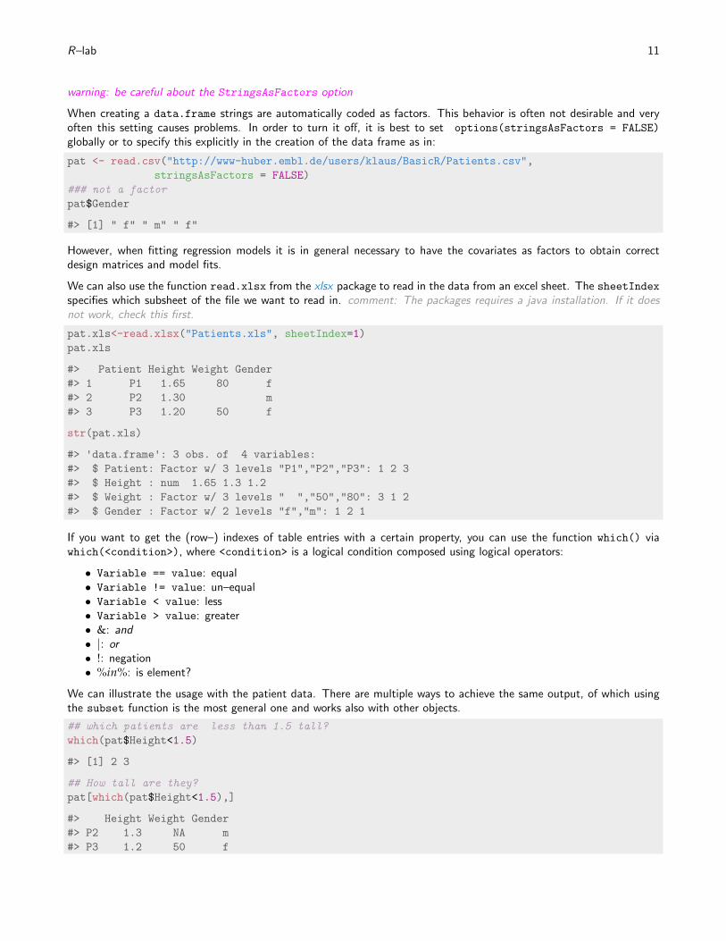
warning: be careful about the StringsAsFactors option
When creating a data.frame strings are automatically coded as factors. This behavior is often not desirable and veryoften this setting causes problems. In order to turn it off, it is best to set options(stringsAsFactors = FALSE)
globally or to specify this explicitly in the creation of the data frame as in:
pat <- read.csv("http://www-huber.embl.de/users/klaus/BasicR/Patients.csv",
stringsAsFactors = FALSE)
### not a factor
pat$Gender
#> [1] " f" " m" " f"
However, when fitting regression models it is in general necessary to have the covariates as factors to obtain correctdesign matrices and model fits.
We can also use the function read.xlsx from the xlsx package to read in the data from an excel sheet. The sheetIndexspecifies which subsheet of the file we want to read in. comment: The packages requires a java installation. If it doesnot work, check this first.
pat.xls<-read.xlsx("Patients.xls", sheetIndex=1)
pat.xls
#> Patient Height Weight Gender
#> 1 P1 1.65 80 f
#> 2 P2 1.30 m
#> 3 P3 1.20 50 f
str(pat.xls)
#> 'data.frame': 3 obs. of 4 variables:
#> $ Patient: Factor w/ 3 levels "P1","P2","P3": 1 2 3
#> $ Height : num 1.65 1.3 1.2
#> $ Weight : Factor w/ 3 levels " ","50","80": 3 1 2
#> $ Gender : Factor w/ 2 levels "f","m": 1 2 1
If you want to get the (row–) indexes of table entries with a certain property, you can use the function which() viawhich(<condition>), where <condition> is a logical condition composed using logical operators:
• Variable == value: equal• Variable != value: un–equal• Variable < value: less• Variable > value: greater• &: and• |: or• !: negation• %in%: is element?
We can illustrate the usage with the patient data. There are multiple ways to achieve the same output, of which usingthe subset function is the most general one and works also with other objects.
## which patients are less than 1.5 tall?
which(pat$Height<1.5)
#> [1] 2 3
## How tall are they?
pat[which(pat$Height<1.5),]
#> Height Weight Gender
#> P2 1.3 NA m
#> P3 1.2 50 f
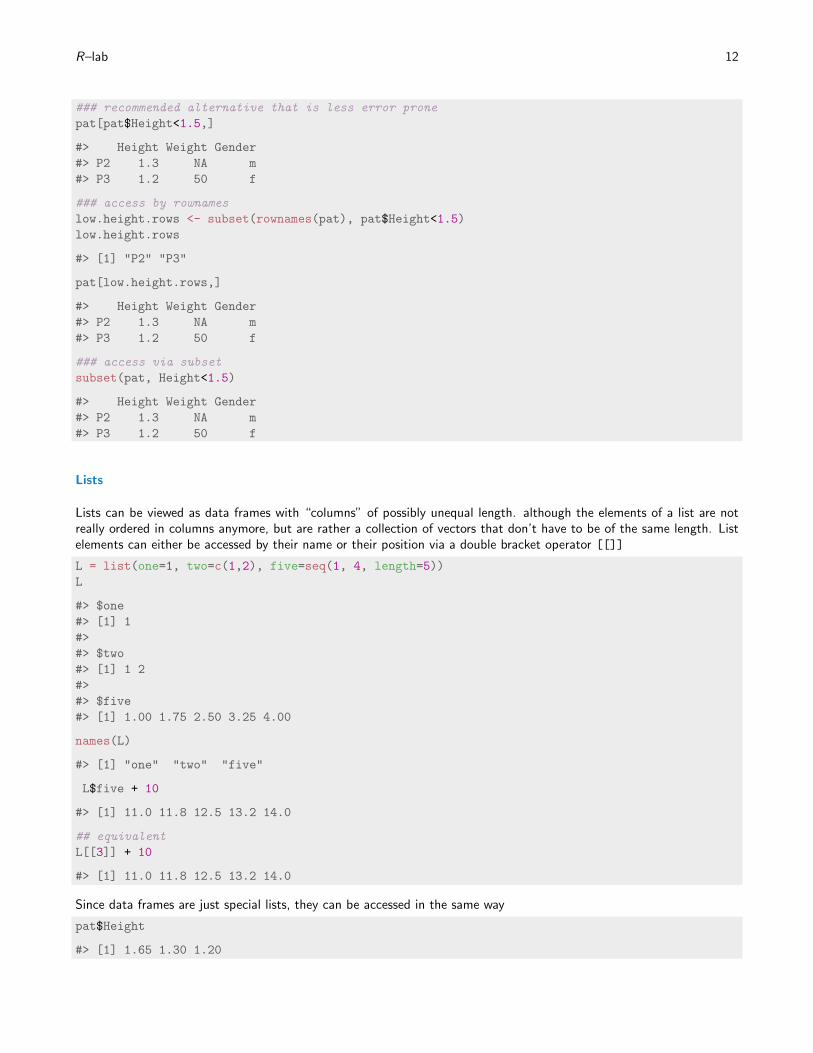
R–lab 12
### recommended alternative that is less error prone
pat[pat$Height<1.5,]
#> Height Weight Gender
#> P2 1.3 NA m
#> P3 1.2 50 f
### access by rownames
low.height.rows <- subset(rownames(pat), pat$Height<1.5)
low.height.rows
#> [1] "P2" "P3"
pat[low.height.rows,]
#> Height Weight Gender
#> P2 1.3 NA m
#> P3 1.2 50 f
### access via subset
subset(pat, Height<1.5)
#> Height Weight Gender
#> P2 1.3 NA m
#> P3 1.2 50 f
Lists
Lists can be viewed as data frames with “columns” of possibly unequal length. although the elements of a list are notreally ordered in columns anymore, but are rather a collection of vectors that don’t have to be of the same length. Listelements can either be accessed by their name or their position via a double bracket operator [[]]
L = list(one=1, two=c(1,2), five=seq(1, 4, length=5))
L
#> $one
#> [1] 1
#>
#> $two
#> [1] 1 2
#>
#> $five
#> [1] 1.00 1.75 2.50 3.25 4.00
names(L)
#> [1] "one" "two" "five"
L$five + 10
#> [1] 11.0 11.8 12.5 13.2 14.0
## equivalent
L[[3]] + 10
#> [1] 11.0 11.8 12.5 13.2 14.0
Since data frames are just special lists, they can be accessed in the same way
pat$Height
#> [1] 1.65 1.30 1.20
R–lab 13
#equivalent
pat[[1]]
#> [1] 1.65 1.30 1.20
6.3 Apply functions
A very useful class of functions in R are apply commands, which allows to apply a function to every row or column ofa data matrix, data frame or list:
apply(X, MARGIN, FUN, ...)
• MARGIN: 1 (row-wise) or 2 (column-wise)• FUN: The function to apply
The dots argument allows you to specify additional arguments that will be passed to FUN.
Special apply are functions include: lapply (lists), sapply (lapply wrapper trying to convert the result into a vector ormatrix), tapply and aggregate (apply according to factor groups).
We can illustrate this again using the patients data set:
# Calculate mean for each of the first two columns
sapply(X = pat[,1:2], FUN = mean, na.rm = TRUE)
#> Height Weight
#> 1.38 65.00
# Mean height separately for each gender
tapply(X = pat$Height, FUN = mean, INDEX = pat$Ge)
#> f m
#> 1.42 1.30
Data handling can be much more elegantly performed by the plyr and dplyr packages, which will be introduced in anotherlab.
Exercise: Handling a small data set
(a) Read in the data set ’Patients.csv’ from the website
http://www-huber.embl.de/users/klaus/BasicR/Patients.csv
(b) Check whether the read in data is actually a data.frame.(c) Which variables are stored in the data frame and what are their values?(d) Is there a missing weight value? If yes, replace it by the mean of the other weight values.(e) Calculate the mean weight and height of all the patients.(f ) Calculate the BMI = Weight/Height2 of all the patients. Attach the BMI vector to the data frame using the
function cbind.
7 Plotting in R
R–lab 14
7.1 Plotting in base R
The default command for plotting is plot(), there are other specialized commands like hist() or pie(). A collection ofsuch specialized commands (e.g. heatmaps and CI plots) can be found in the package gplots. Another useful visualizationpackage is LSD, which includes a heat–scatterplot. The general plot command looks like this:
plot(x, y, type, main, par (...) )
• x: x–axis data• y: y–axis data (may be missing)• type=l,p,h,b display lines / points / horizontal lines ...• main: plot heading• par (...) additional graphical parameters, see ?par for more info . . .
The function plot() creates the plot. Additional lines, points and so on can be added by R commands of the samename: lines() and points(). The command pdf will open a pdf document as a “graphical device”, subsequentlyeverything will be plotted to the pdf. With dev.off() the device will be closed and the pdf will be viewable. A newgraphical device can be opened by dev.new(). This allows you to create a new plot without overwriting the current ac-tive one. With the graphical option par ( mfrow=c(<no.rows>, <no.columns>) ) you can produce an array of plots.
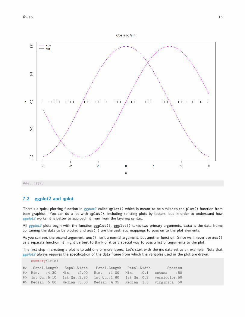
As a comprehensive example, the following code produces a sine / cosine plot and colors it:
#pdf(file="plot-example.pdf", width=12, height=6)
x <- seq(-3,3, by = 0.1); y <- cos(x); z <- sin(x)
plot(x,y, type="l", col="darkviolet", main="Cos and Sin")
points(x, rep(0, length(x)), pch=3)
lines(x,z, type="l", col="magenta")
legend("topleft", c("cos","sin"), col=c("darkviolet",
"magenta"), lty=1)
R–lab 15
#dev.off()
7.2 ggplot2 and qplot
There’s a quick plotting function in ggplot2 called qplot() which is meant to be similar to the plot() function frombase graphics. You can do a lot with qplot(), including splitting plots by factors, but in order to understand howggplot2 works, it is better to approach it from from the layering syntax.
All ggplot2 plots begin with the function ggplot(). ggplot() takes two primary arguments, data is the data framecontaining the data to be plotted and aes( ) are the aesthetic mappings to pass on to the plot elements.
As you can see, the second argument, aes(), isn’t a normal argument, but another function. Since we’ll never use aes()
as a separate function, it might be best to think of it as a special way to pass a list of arguments to the plot.
The first step in creating a plot is to add one or more layers. Let’s start with the iris data set as an example. Note thatggplot2 always requires the specification of the data frame from which the variables used in the plot are drawn.
summary(iris)
#> Sepal.Length Sepal.Width Petal.Length Petal.Width Species
#> Min. :4.30 Min. :2.00 Min. :1.00 Min. :0.1 setosa :50
#> 1st Qu.:5.10 1st Qu.:2.80 1st Qu.:1.60 1st Qu.:0.3 versicolor:50
#> Median :5.80 Median :3.00 Median :4.35 Median :1.3 virginica :50
R–lab 16
#> Mean :5.84 Mean :3.06 Mean :3.76 Mean :1.2
#> 3rd Qu.:6.40 3rd Qu.:3.30 3rd Qu.:5.10 3rd Qu.:1.8
#> Max. :7.90 Max. :4.40 Max. :6.90 Max. :2.5
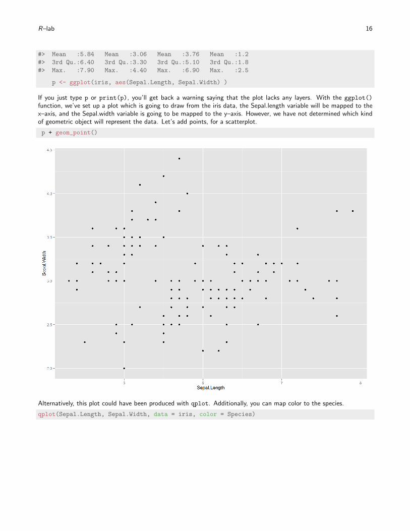
p <- ggplot(iris, aes(Sepal.Length, Sepal.Width) )
If you just type p or print(p), you’ll get back a warning saying that the plot lacks any layers. With the ggplot()
function, we’ve set up a plot which is going to draw from the iris data, the Sepal.length variable will be mapped to thex–axis, and the Sepal.width variable is going to be mapped to the y–axis. However, we have not determined which kindof geometric object will represent the data. Let’s add points, for a scatterplot.
p + geom_point()
Alternatively, this plot could have been produced with qplot. Additionally, you can map color to the species.
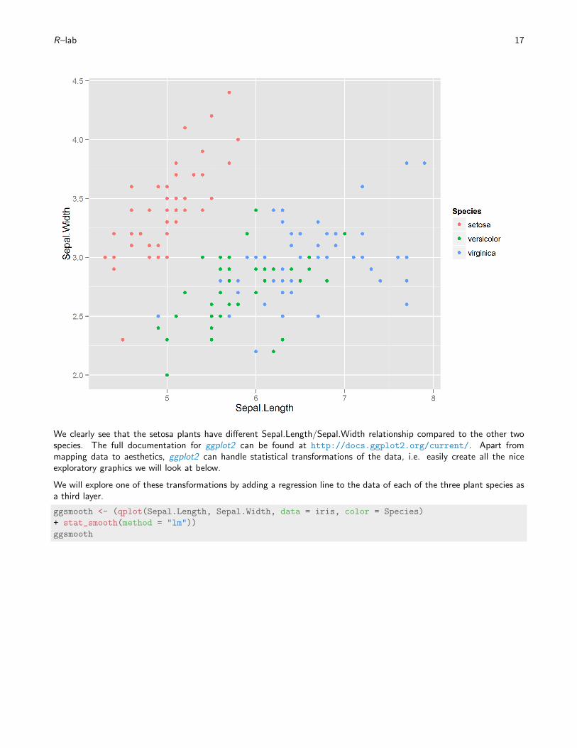
qplot(Sepal.Length, Sepal.Width, data = iris, color = Species)
R–lab 17
We clearly see that the setosa plants have different Sepal.Length/Sepal.Width relationship compared to the other twospecies. The full documentation for ggplot2 can be found at http://docs.ggplot2.org/current/. Apart frommapping data to aesthetics, ggplot2 can handle statistical transformations of the data, i.e. easily create all the niceexploratory graphics we will look at below.
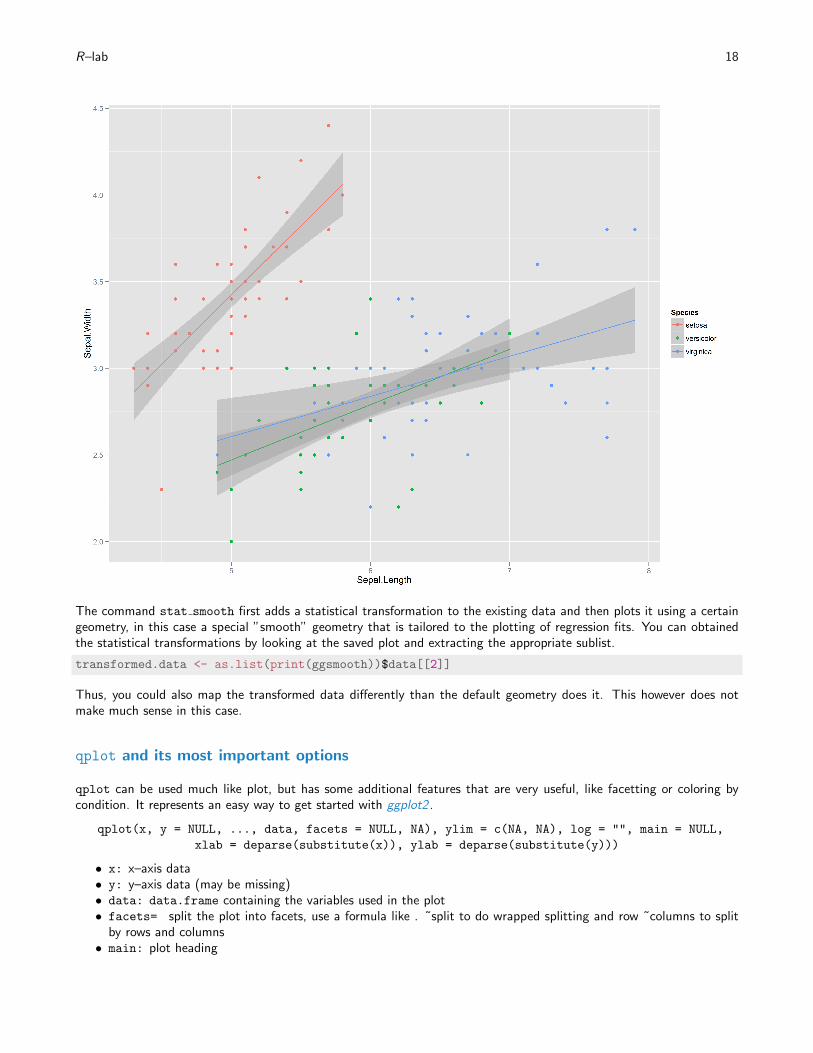
We will explore one of these transformations by adding a regression line to the data of each of the three plant species asa third layer.
ggsmooth <- (qplot(Sepal.Length, Sepal.Width, data = iris, color = Species)
+ stat_smooth(method = "lm"))
ggsmooth
R–lab 18
The command stat smooth first adds a statistical transformation to the existing data and then plots it using a certaingeometry, in this case a special ”smooth” geometry that is tailored to the plotting of regression fits. You can obtainedthe statistical transformations by looking at the saved plot and extracting the appropriate sublist.
transformed.data <- as.list(print(ggsmooth))$data[[2]]
Thus, you could also map the transformed data differently than the default geometry does it. This however does notmake much sense in this case.
qplot and its most important options
qplot can be used much like plot, but has some additional features that are very useful, like facetting or coloring bycondition. It represents an easy way to get started with ggplot2 .
qplot(x, y = NULL, ..., data, facets = NULL, NA), ylim = c(NA, NA), log = "", main = NULL,
xlab = deparse(substitute(x)), ylab = deparse(substitute(y)))
• x: x–axis data• y: y–axis data (may be missing)• data: data.frame containing the variables used in the plot• facets= split the plot into facets, use a formula like . ˜split to do wrapped splitting and row ˜columns to split
by rows and columns• main: plot heading
R–lab 19
• color, fill set to factor/string in the data set in order to color the plot depending on that factor. UseI("colorname") to use a specific color.
• geom specify a “geometry” to be used in the plots, examples include point, line, boxplot, histogram etc.• xlab, ylab, xlim, ylim set the x–/y–axis parameters
Exercise: Plotting the normal density
The density of the normal distribution with expected value µ and variance σ2 is given by:
f (x) =1
σ2√
πexp
(−1
2(
x− µ
σ)2)
In R it is implemented in the function dnorm.
(a) Call the R help to find out how to calculate density values.(b) Determine the values of the standard normal distribution density (µ = 0 and σ2 = 1) at −2,−1.8,−1.6, . . . ,+2
and save it in a vector stand.normal.(c) Plot the results obtained in the last exercise, play a bit with the plotting options!(d) use qplot to produce the same plot and change the color of the density line using color=I("darkgreen").
8 Calling functions and programming
8.1 Calling functions
Every R–function is following the pattern below:
function.name(arguments, optional arguments)
• arguments: Some function arguments are necessary to run the function• optional arguments: Some function arguments can be changed, otherwise the default values are used. They
are indicated by an equals sign.• ?function.name: Getting help• function.name: Source code
As an example, look at the mean command:
mean(x, trim = 0, na.rm = FALSE)
• x: Data• trim = 0: Trimmed mean (mean of the data without x% of extreme values)• na.rm = FALSE: Remove missing values?
Here, x (usually a vector) has to be given in order to run the function, while the other arguments such as trim areoptional, i.e. if you do not change them, their default values are used.
8.2 Creating your own functions
You can create your own functions very easily by adhering to the following template
function.name<-function(arguments, options) {...
...
return(...) }
R–lab 20
• { } : The source code of the function has to be in curly brackets• By default R returns the result of the last line of the function, you can specify the return value directly withreturn( ). If you want to return multiple values, you can return a list.
As example, we look at the following currency converter function
euro.calc<-function(x, currency="US") {## currency has a default argrument "US"
if(currency=="US") return(x*1.33)
if(currency=="Pounds") return(x*0.85)
}euro.calc(100) ## how many dollars are 100 Euros?
#> [1] 133
Here x is a formal argument, necessary to execute the function. currency: is an optional argument, set to “US” bydefault.
8.3 Flow control
R offers the typical options for flow–control known from many other languages.
The most important one, the if–statement is used when certain computations should only be performed if a certaincondition is met (and maybe something else should be performed when the condition is not met):
w= 3
if( w < 5 ){d=2
}else{d=10
}d
#> [1] 2
If you want do a computation for every entry of a list, you usually do the computations for one time step and then forthe next and the next, etc. Because nobody wants to type the same commands over and over again, these computationsare automated in for–loops. An example:
h <- seq(from = 1, to = 8)
s <- integer() # create empty integer vector
for(i in 2:10)
{s[i] <- h[i] * 10
}s
#> [1] NA 20 30 40 50 60 70 80 NA NA
Another useful command is the ifelse–command, it replaces elements of a vector based on the evaluation of anotherlogical vector of the same size. This is useful to replace missing values, or to binarize a vector.
s <- seq(from = 1, to = 10)
binary.s <- ifelse(s > 5, "high", "low")
binary.s
#> [1] "low" "low" "low" "low" "low" "high" "high" "high" "high" "high"
R–lab 21
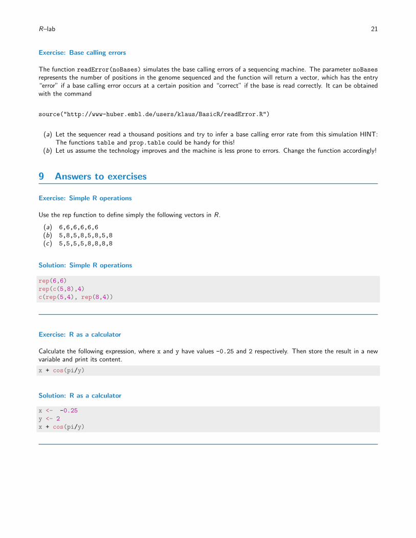
Exercise: Base calling errors
The function readError(noBases) simulates the base calling errors of a sequencing machine. The parameter noBasesrepresents the number of positions in the genome sequenced and the function will return a vector, which has the entry“error” if a base calling error occurs at a certain position and “correct” if the base is read correctly. It can be obtainedwith the command
source("http://www-huber.embl.de/users/klaus/BasicR/readError.R")
(a) Let the sequencer read a thousand positions and try to infer a base calling error rate from this simulation HINT:The functions table and prop.table could be handy for this!
(b) Let us assume the technology improves and the machine is less prone to errors. Change the function accordingly!
9 Answers to exercises
Exercise: Simple R operations
Use the rep function to define simply the following vectors in R.
(a) 6,6,6,6,6,6
(b) 5,8,5,8,5,8,5,8
(c) 5,5,5,5,8,8,8,8
Solution: Simple R operations
rep(6,6)
rep(c(5,8),4)
c(rep(5,4), rep(8,4))
Exercise: R as a calculator
Calculate the following expression, where x and y have values -0.25 and 2 respectively. Then store the result in a newvariable and print its content.
x + cos(pi/y)
Solution: R as a calculator
x <- -0.25
y <- 2
x + cos(pi/y)
R–lab 22
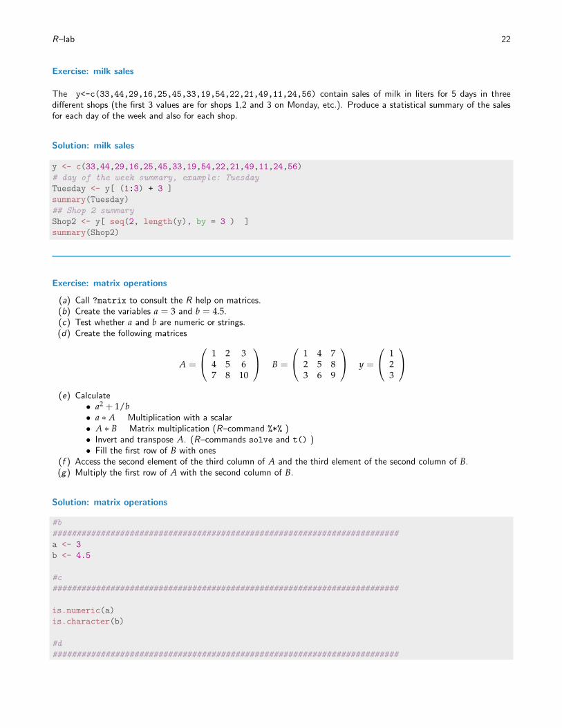
Exercise: milk sales
The y<-c(33,44,29,16,25,45,33,19,54,22,21,49,11,24,56) contain sales of milk in liters for 5 days in threedifferent shops (the first 3 values are for shops 1,2 and 3 on Monday, etc.). Produce a statistical summary of the salesfor each day of the week and also for each shop.
Solution: milk sales
y <- c(33,44,29,16,25,45,33,19,54,22,21,49,11,24,56)
# day of the week summary, example: Tuesday
Tuesday <- y[ (1:3) + 3 ]
summary(Tuesday)
## Shop 2 summary
Shop2 <- y[ seq(2, length(y), by = 3 ) ]
summary(Shop2)
Exercise: matrix operations
(a) Call ?matrix to consult the R help on matrices.(b) Create the variables a = 3 and b = 4.5.(c) Test whether a and b are numeric or strings.(d) Create the following matrices
A =
1 2 34 5 67 8 10
B =
1 4 72 5 83 6 9
y =
123
(e) Calculate
• a2 + 1/b• a ∗ A Multiplication with a scalar• A ∗ B Matrix multiplication (R–command %*% )• Invert and transpose A. (R–commands solve and t() )• Fill the first row of B with ones
(f ) Access the second element of the third column of A and the third element of the second column of B.(g) Multiply the first row of A with the second column of B.
Solution: matrix operations
#b
########################################################################
a <- 3
b <- 4.5
#c
########################################################################
is.numeric(a)
is.character(b)
#d
########################################################################
R–lab 23
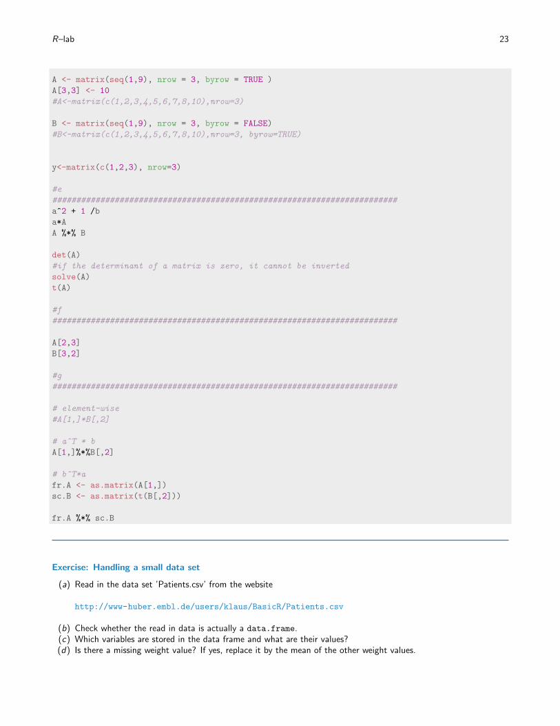
A <- matrix(seq(1,9), nrow = 3, byrow = TRUE )
A[3,3] <- 10
#A<-matrix(c(1,2,3,4,5,6,7,8,10),nrow=3)
B <- matrix(seq(1,9), nrow = 3, byrow = FALSE)
#B<-matrix(c(1,2,3,4,5,6,7,8,10),nrow=3, byrow=TRUE)
y<-matrix(c(1,2,3), nrow=3)
#e
########################################################################
a^2 + 1 /b
a*A
A %*% B
det(A)
#if the determinant of a matrix is zero, it cannot be inverted
solve(A)
t(A)
#f
########################################################################
A[2,3]
B[3,2]
#g
########################################################################
# element-wise
#A[1,]*B[,2]
# a^T * b
A[1,]%*%B[,2]
# b^T*a
fr.A <- as.matrix(A[1,])
sc.B <- as.matrix(t(B[,2]))
fr.A %*% sc.B
Exercise: Handling a small data set
(a) Read in the data set ’Patients.csv’ from the website
http://www-huber.embl.de/users/klaus/BasicR/Patients.csv
(b) Check whether the read in data is actually a data.frame.(c) Which variables are stored in the data frame and what are their values?(d) Is there a missing weight value? If yes, replace it by the mean of the other weight values.
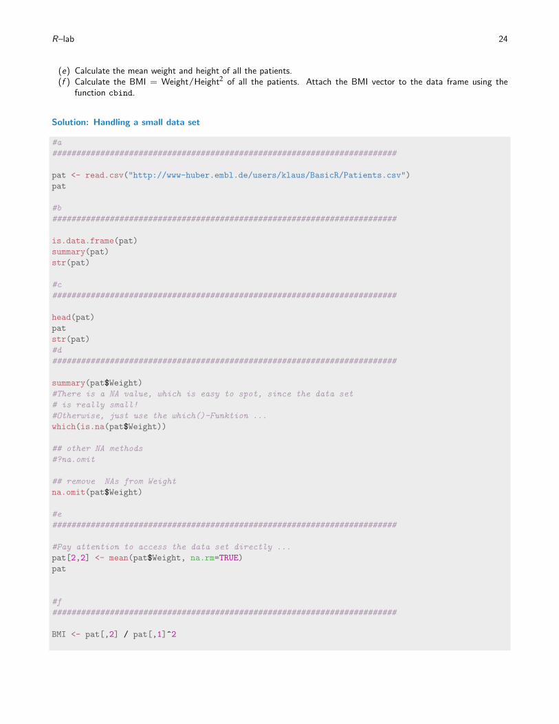
R–lab 24
(e) Calculate the mean weight and height of all the patients.(f ) Calculate the BMI = Weight/Height2 of all the patients. Attach the BMI vector to the data frame using the
function cbind.
Solution: Handling a small data set
#a
########################################################################
pat <- read.csv("http://www-huber.embl.de/users/klaus/BasicR/Patients.csv")
pat
#b
########################################################################
is.data.frame(pat)
summary(pat)
str(pat)
#c
########################################################################
head(pat)
pat
str(pat)
#d
########################################################################
summary(pat$Weight)
#There is a NA value, which is easy to spot, since the data set
# is really small!
#Otherwise, just use the which()-Funktion ...
which(is.na(pat$Weight))
## other NA methods
#?na.omit
## remove NAs from Weight
na.omit(pat$Weight)
#e
########################################################################
#Pay attention to access the data set directly ...
pat[2,2] <- mean(pat$Weight, na.rm=TRUE)
pat
#f
########################################################################
BMI <- pat[,2] / pat[,1]^2
R–lab 25
### alternatively
BMI = pat$Weight / pat$Height^2
pat$Weight[2] = mean(pat$Weight, na.rm=TRUE)
print(BMI)
### attach BMI to the data frame
pat <- cbind(pat, BMI)
pat
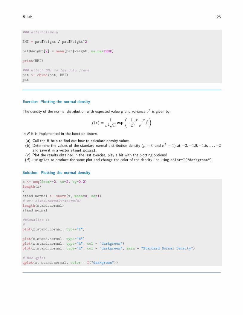
Exercise: Plotting the normal density
The density of the normal distribution with expected value µ and variance σ2 is given by:
f (x) =1
σ2√
πexp
(−1
2(
x− µ
σ)2)
In R it is implemented in the function dnorm.
(a) Call the R help to find out how to calculate density values.(b) Determine the values of the standard normal distribution density (µ = 0 and σ2 = 1) at −2,−1.8,−1.6, . . . ,+2
and save it in a vector stand.normal.(c) Plot the results obtained in the last exercise, play a bit with the plotting options!(d) use qplot to produce the same plot and change the color of the density line using color=I("darkgreen").
Solution: Plotting the normal density
x <- seq(from=-2, to=2, by=0.2)
length(x)
x
stand.normal <- dnorm(x, mean=0, sd=1)
# or: stand.normal<-dnorm(x)
length(stand.normal)
stand.normal
#visualize it
#
plot(x,stand.normal, type="l")
plot(x,stand.normal, type="b")
plot(x,stand.normal, type="h", col = "darkgreen")
plot(x,stand.normal, type="h", col = "darkgreen", main = "Standard Normal Density")
# use qplot
qplot(x, stand.normal, color = I("darkgreen"))
R–lab 26
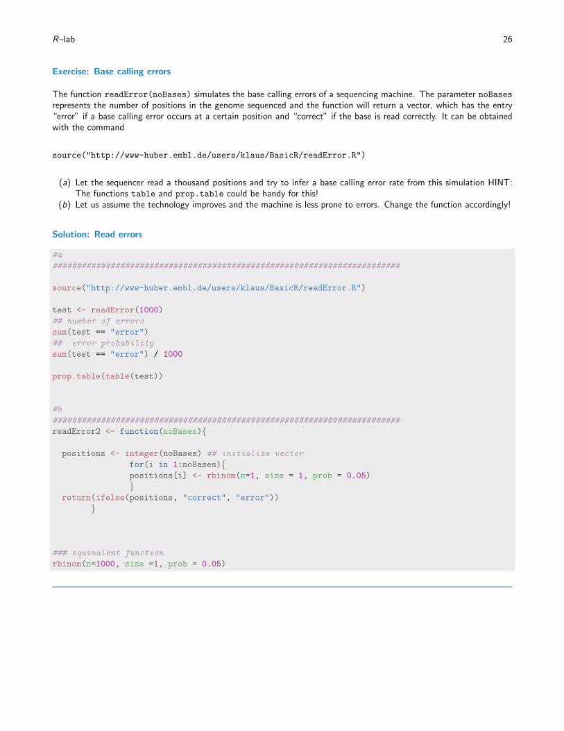
Exercise: Base calling errors
The function readError(noBases) simulates the base calling errors of a sequencing machine. The parameter noBasesrepresents the number of positions in the genome sequenced and the function will return a vector, which has the entry“error” if a base calling error occurs at a certain position and “correct” if the base is read correctly. It can be obtainedwith the command
source("http://www-huber.embl.de/users/klaus/BasicR/readError.R")
(a) Let the sequencer read a thousand positions and try to infer a base calling error rate from this simulation HINT:The functions table and prop.table could be handy for this!
(b) Let us assume the technology improves and the machine is less prone to errors. Change the function accordingly!
Solution: Read errors
#a
########################################################################
source("http://www-huber.embl.de/users/klaus/BasicR/readError.R")
test <- readError(1000)
## number of errors
sum(test == "error")
## error probability
sum(test == "error") / 1000
prop.table(table(test))
#b
########################################################################
readError2 <- function(noBases){
positions <- integer(noBases) ## initialize vector
for(i in 1:noBases){positions[i] <- rbinom(n=1, size = 1, prob = 0.05)
}return(ifelse(positions, "correct", "error"))
}
### equivalent function
rbinom(n=1000, size =1, prob = 0.05)

R–lab 27
Session Info
toLatex(sessionInfo())
• R version 3.2.0 (2015-04-16), x86_64-w64-mingw32• Locale: LC_COLLATE=English_United States.1252, LC_CTYPE=English_United States.1252,LC_MONETARY=English_United States.1252, LC_NUMERIC=C, LC_TIME=English_United States.1252
• Base packages: base, datasets, graphics, grDevices, methods, parallel, stats, utils• Other packages: Biobase 2.28.0, BiocGenerics 0.14.0, BiocInstaller 1.18.1, dplyr 0.4.1, ggplot2 1.0.1, knitr 1.10,
magrittr 1.5, mgcv 1.8-6, multtest 2.24.0, nlme 3.1-120, plyr 1.8.2, reshape2 1.4.1, rJava 0.9-6, stringr 0.6.2,TeachingDemos 2.9, tidyr 0.2.0, xlsx 0.5.7, xlsxjars 0.6.1
• Loaded via a namespace (and not attached): assertthat 0.1, BiocStyle 1.6.0, codetools 0.2-11, colorspace 1.2-6,DBI 0.3.1, digest 0.6.8, evaluate 0.7, formatR 1.2, grid 3.2.0, gtable 0.1.2, highr 0.5, labeling 0.3, lattice 0.20-31,lazyeval 0.1.10, MASS 7.3-40, Matrix 1.2-0, munsell 0.4.2, proto 0.3-10, R6 2.0.1, Rcpp 0.11.5, scales 0.2.4,splines 3.2.0, stats4 3.2.0, survival 2.38-1, tools 3.2.0