Lab: Machine Learning, Part I

R. Gentleman, W, Huber, V. Carey, R. Irizarry

October 6, 2006

Introduction

In this lab we will cover some of the basic principles of machine learning. We will use theALL data set and will work on two different problems. For one of them it is relativelyeasy to classify the samples and for the other, it is harder.

Fundamental to the task of machine learning is selecting a distance. In many cases itis more important than the choice of classification method (you might want to try somedifferent choices for distances in the problems below and see what changes).

Feature selection is also an important problem. We suggest that you take a simpleapproach and use genes which are differentially expressed between the phenotypes understudy. In some cases this can be improved on, but in general it seems to be a reasonableapproach.

In most cases we have no a priori reason to believe that any one gene should get moreweighting than another. If that is true, then we must standardize the genes beforecarrying out machine learning. If we do not standardize them (for each gene, subtractsome measure of the center and divide by some measure of the variability across samples),then many machine learning algorithms (and distances) will treat different genes quitedifferently, typically depending on their observed mean expression level and its variationacross samples. So, standardization is recommended, however, it raises an importantprerequisite:

If you decide to standardize your expression data you will need to perform some sort ofnon-specific filtering to remove genes that have low variability, for example because theyare not expressed, or because the microarray experiment did not work for these genes dueto low labeling or hybridization efficiencies. The reason you must do this is that we donot want to amplify what is essentially “noise” by the operation of standardization.

1

Machine Learning Check List

1. Filter out features (genes) which show little variation across samples, or which areknown not to be of interest. If appropriate transform features to all be on the samescale.

2. Select a distance measure. What does it mean to be close?

3. Feature selection: select features to be used for machine learning.

4. Select the algorithm: which of the very many machine learning algorithms do youwant to use?

5. Assess the performance of your classifier. Typically this is done using cross-validation.

Non-specific filtering

First load the Biobase and ALL packages and then use the data function to load the ALL

data. Since the data in ALL are large and phenotypically quite diverse, we reduce the casesdown to a reasonable two group comparison. We will return to a multigroup comparisonlater.

> library("Biobase")

> library("ALL")

> data(ALL, package = "ALL")

> ALLBs = ALL[, grep("^B", as.character(ALL$BT))]

> ALLBCRNEG = ALLBs[, ALLBs$mol == "BCR/ABL" | ALLBs$mol == "NEG"]

> ALLBCRNEG$mol.biol = factor(ALLBCRNEG$mol.biol)

> numBN = length(ALLBCRNEG$mol.biol)

> ALLBCRALL1 = ALLBs[, ALLBs$mol == "BCR/ABL" | ALLBs$mol == "ALL1/AF4"]

> ALLBCRALL1$mol.biol = factor(ALLBCRALL1$mol.biol)

> numBA = length(ALLBCRALL1$mol.biol)

Question 1How many samples are in the BCR/ABL-NEG subset? How many are in the BCR/ABL-ALL1/AF4 subset?

You now have two data sets to work with. Most of the code for carrying out machinelearning can easily be applied to either data set. The comparison of BCR/ABL to NEG isdifficult, and the error rates are typically quite high. On the other hand, the comparisonof BCR/ABL to ALL1/AF4 is rather easy, and the error rates should be small.

In this lab we will first select some genes to use as features for the rest of the lab. Nextwe will use those features to do some machine learning, in particular we will make use

2

of cross-validation to select parameters of the classification model and see how to assessthe model itself. Many of the details can be explored in much more detail, and somesuggestions are made.

Preprocessing

First carry out non-specific filtering, as described in the Differential Expression Lab. Youshould remove those genes that you think are not sufficiently informative to be consideredfurther. One recommendation is to filter on variability.

Here, we take the simplistic approach of using the 75th percentile of the interquartilerange (IQR) as the cut-off point. We do this because we want to have relatively fewgenes to deal with so the examples will run quickly on laptops. Finding the IQR can bedone either by applying the IQR function over all rows of the exprSet , or by manuallycomputing quantiles using the very fast function rowQ (there are some slight, hardlyrelevant numerical differences).

> lowQ = rowQ(ALLBCRNEG, floor(0.25 * numBN))

> upQ = rowQ(ALLBCRNEG, ceiling(0.75 * numBN))

> iqrs = upQ - lowQ

> giqr = iqrs > quantile(iqrs, probs = 0.75)

> sum(giqr)

[1] 3156

> BNsub = ALLBCRNEG[giqr, ]

Exercise 1What kind of object is BNsub?

Selecting a Distance

To some extent your choices here are not always that flexible because many machinelearning algorithms have the distance measure fixed in advance.

There are a number of different tools that you can use in R to compute the distancebetween objects. They include the function dist, the function daisy from the clusterpackage (Kaufman and Rousseeuw, 1990), and the functions in the bioDist package. ThebioDist package is discussed in Chapter 12 of Gentleman et al. (2005). Some ideas onvisualizing distance measures can be found in Section 10.5 of that same reference.

3

Exercise 2What distance measures are availble in the bioDist package? Hint: load the package andthen look at the loaded functions, or read the vignette.

To make the computations easier, we take the first sixty genes from the BNsub data setand use those for the exercises in this section. The dist function computes the distancebetween rows of an input matrix. Since we want the distances between samples, wetranspose the matrix using the function t. The return value is an instance of the distclass and you should read the manual page carefully to find out more about this class.Since this class is not supported by some R functions we will want to use, we also convertit to a matrix.

> dSub <- BNsub[1:60, ]

> eucD <- dist(t(exprs(dSub)))

> eucD@Size

[1] 79

> eucM <- as.matrix(eucD)

We can use this as an input to various clustering algorithms and plot the outputs. Butfor now we want to visualize it as a heatmap.

> library("RColorBrewer")

> hmcol <- colorRampPalette(brewer.pal(10, "RdBu"))(256)

> heatmap(eucM, sym = TRUE, col = hmcol, distfun = function(x) as.dist(x))

Question 2What do you notice most about the heatmap?

Since our goal is to introduce you to a number of different distances and to help youunderstand their effects, visualization is important. We will also create a few helperfunctions to make it easier to carry out certain transformations and calculations. Firstwe define a function to find the closest neighbor of a particular observation given adistance matrix and a label specifying an observation in the distance matrix.

> closestN = function(distM, label) {

+ loc = match(label, row.names(distM))

+ names(which.min(distM[label, -loc]))

+ }

> closestN(eucM, "03002")

4

4300

427

004

4301

212

006

2401

028

001

2700

328

042

2802

328

019

0401

030

001

2802

128

035

2803

728

047

2800

628

036

2804

328

044

2802

424

018

3600

222

009

2800

528

031

2800

743

007

0801

249

006

0401

604

008

1500

168

003

4300

116

009

0101

024

017

6400

220

002

6800

125

006

3300

548

001

0900

815

005

6200

112

026

1401

637

013

1201

257

001

3101

122

010

6200

224

022

6200

326

003

0901

711

005

0801

112

019

2401

122

013

0300

224

008

8400

408

001

0400

725

003

2400

108

024

2201

106

002

6400

165

005

2600

101

005

1200

7

12007010052600165005640010600222011080242400125003040070800184004240080300222013240111201908011110050901726003620032402262002220103101157001120123701314016120266200115005090084800133005250066800120002640022401701010160094300168003150010400804016490060801243007280072803128005220093600224018280242804428043280362800628047280372803528021300010401028019280232804227003280012401012006430122700443004

Figure 1: A heatmap of the between-sample distances.

5

[1] "22013"

Exercise 3Compute the distance between the samples using the MIdist function from the bioDistpackage. What distance does this function compute? Which sample is closest to "03002"

in this distance?

Feature Selection

Now we are ready to select features. Perhaps the easiest approach to feature selection isto use a t-test.

> library("genefilter")

> tt1 = rowttests(BNsub, "mol.biol")

> numToSel <- 50

Using the t-test statistics, we will select the top 50 genes to use for the machine learningquestions below.

> tt1ord = order(abs(tt1$statistic), decreasing = TRUE)

> top50 = tt1ord[1:numToSel]

> BNsub1 = BNsub[top50, ]

Exercise 4What is the value of the largest t-statistic? Which gene does it correspond to? What isthe corresponding p-value?

Next we will standardize all gene expression values. As discussed above, it is importantthat non-specific filtering has already been applied, otherwise the standardization stepwill add unnecessary noise to the data.

Since we will compute IQR by row many times in the next code chunk, we first write ahelper function to compute this for us. The only tricky issue is that we want our helperto be able to handle instances of the exprSet or matrix classes.

> rowIQRs = function(eSet) {

+ if (is(eSet, "exprSet"))

+ numSamp = length(sampleNames(eSet))

+ else numSamp = ncol(eSet)

+ lowQ = rowQ(eSet, floor(0.25 * numSamp))

+ upQ = rowQ(eSet, ceiling(0.75 * numSamp))

+ upQ - lowQ

+ }

6

Exercise 5Use the rowIQRs function to repeat the IQR calculation that was carried out previously.Do you get the same values?

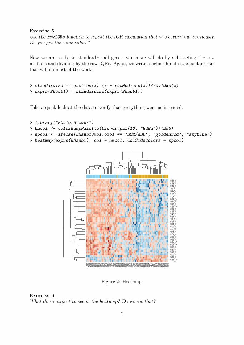
Now we are ready to standardize all genes, which we will do by subtracting the rowmedians and dividing by the row IQRs. Again, we write a helper function, standardize,that will do most of the work.

> standardize = function(x) (x - rowMedians(x))/rowIQRs(x)

> exprs(BNsub1) = standardize(exprs(BNsub1))

Take a quick look at the data to verify that everything went as intended.

> library("RColorBrewer")

> hmcol <- colorRampPalette(brewer.pal(10, "RdBu"))(256)

> spcol <- ifelse(BNsub1$mol.biol == "BCR/ABL", "goldenrod", "skyblue")

> heatmap(exprs(BNsub1), col = hmcol, ColSideColors = spcol)

0400

806

002

1500

124

008

1600

925

006

3300

528

031

2802

304

010

2802

408

012

2201

124

001

0401

628

042

4301

226

001

2401

812

019

2800

768

001

5700

164

002

0802

428

047

2200

925

003

4800

122

010

0101

028

005

6400

128

006

2800

128

037

4300

428

043

4300

704

007

3600

228

019

2803

528

044

2401

709

008

3000

128

021

6500

522

013

8400

420

002

2700

312

012

0300

262

001

2402

228

036

2600

362

002

1100

508

011

2401

101

005

6200

312

007

1202

614

016

3701

349

006

2700

468

003

1200

609

017

1500

543

001

2401

031

011

0800

1

40132_g_at32310_f_at40076_at37014_at40202_at40516_at33774_at32542_at36591_at39329_at39330_s_at39319_at40167_s_at37027_at33232_at40855_at37403_at106_at32434_at2039_s_at40480_s_at32562_at32979_at39824_at39730_at1636_g_at1635_at36275_at1674_at33440_at34472_at33362_at40504_at35162_s_at41815_at37363_at39631_at39837_s_at40196_at671_at40051_at31786_at38032_at1326_at1467_at36617_at35912_at32134_at40795_at37015_at

Figure 2: Heatmap.

Exercise 6What do we expect to see in the heatmap? Do we see that?

7

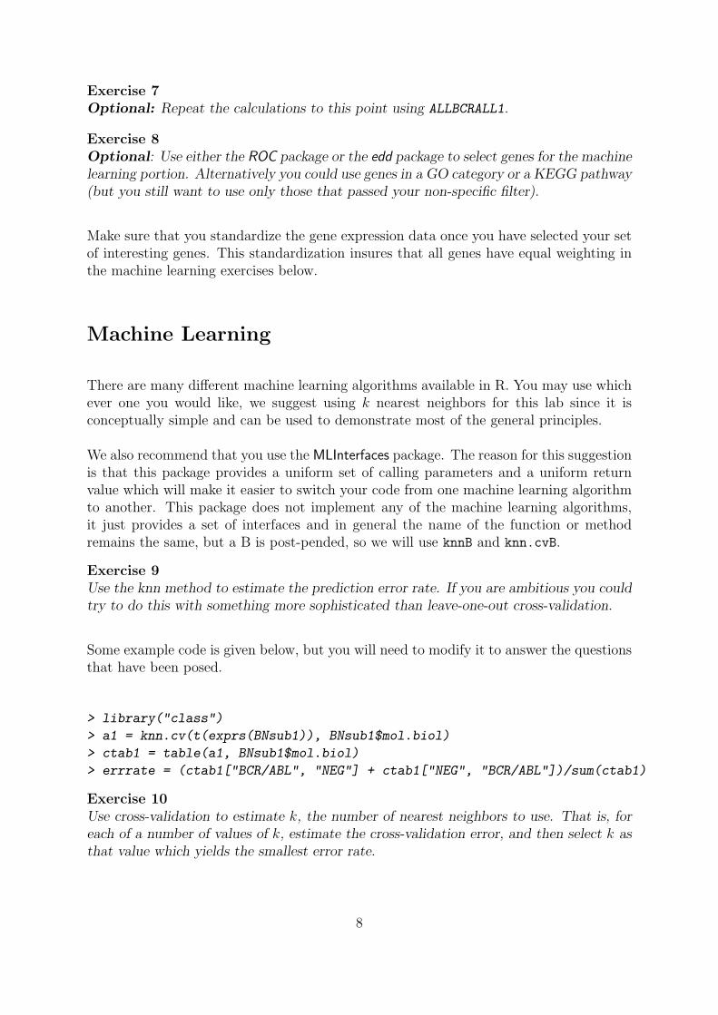
Exercise 7Optional: Repeat the calculations to this point using ALLBCRALL1.

Exercise 8Optional: Use either the ROC package or the edd package to select genes for the machinelearning portion. Alternatively you could use genes in a GO category or a KEGG pathway(but you still want to use only those that passed your non-specific filter).

Make sure that you standardize the gene expression data once you have selected your setof interesting genes. This standardization insures that all genes have equal weighting inthe machine learning exercises below.

Machine Learning

There are many different machine learning algorithms available in R. You may use whichever one you would like, we suggest using k nearest neighbors for this lab since it isconceptually simple and can be used to demonstrate most of the general principles.

We also recommend that you use the MLInterfaces package. The reason for this suggestionis that this package provides a uniform set of calling parameters and a uniform returnvalue which will make it easier to switch your code from one machine learning algorithmto another. This package does not implement any of the machine learning algorithms,it just provides a set of interfaces and in general the name of the function or methodremains the same, but a B is post-pended, so we will use knnB and knn.cvB.

Exercise 9Use the knn method to estimate the prediction error rate. If you are ambitious you couldtry to do this with something more sophisticated than leave-one-out cross-validation.

Some example code is given below, but you will need to modify it to answer the questionsthat have been posed.

> library("class")

> a1 = knn.cv(t(exprs(BNsub1)), BNsub1$mol.biol)

> ctab1 = table(a1, BNsub1$mol.biol)

> errrate = (ctab1["BCR/ABL", "NEG"] + ctab1["NEG", "BCR/ABL"])/sum(ctab1)

Exercise 10Use cross-validation to estimate k, the number of nearest neighbors to use. That is, foreach of a number of values of k, estimate the cross-validation error, and then select k asthat value which yields the smallest error rate.

8

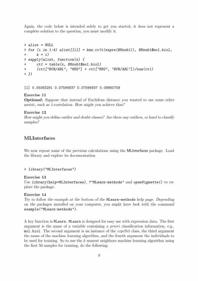
Again, the code below is intended solely to get you started, it does not represent acomplete solution to the question, you must modify it.

> alist = NULL

> for (i in 1:4) alist[[i]] = knn.cv(t(exprs(BNsub1)), BNsub1$mol.biol,

+ k = i)

> sapply(alist, function(x) {

+ ct1 = table(x, BNsub1$mol.biol)

+ (ct1["BCR/ABL", "NEG"] + ct1["NEG", "BCR/ABL"])/sum(ct1)

+ })

[1] 0.05063291 0.07594937 0.07594937 0.08860759

Exercise 11Optional: Suppose that instead of Euclidean distance you wanted to use some othermetric, such as 1-correlation. How might you achieve that?

Exercise 12How might you define outlier and doubt classes? Are there any outliers, or hard to classifysamples?

MLInterfaces

We now repeat some of the previous calculations using the MLInterfaces package. Loadthe library and explore its documentation.

> library("MLInterfaces")

Exercise 13Use library(help=MLInterfaces), ?"MLearn-methods" and openVignette() to ex-plore the package.

Exercise 14Try to follow the example at the bottom of the MLearn-methods help page. Dependingon the packages installed on your computer, you might have luck with the commandexample("MLearn-methods").

A key function is MLearn. MLearn is designed for easy use with expression data. The firstargument is the name of a variable containing a priori classification information, e.g.,mol.biol. The second argument is an instance of the exprSet class, the third argumentthe name of the machine learning algorithm, and the fourth argument the individuals tobe used for training. So to use the k nearest neighbors machine learning algorithm usingthe first 50 samples for training, do the following:

9

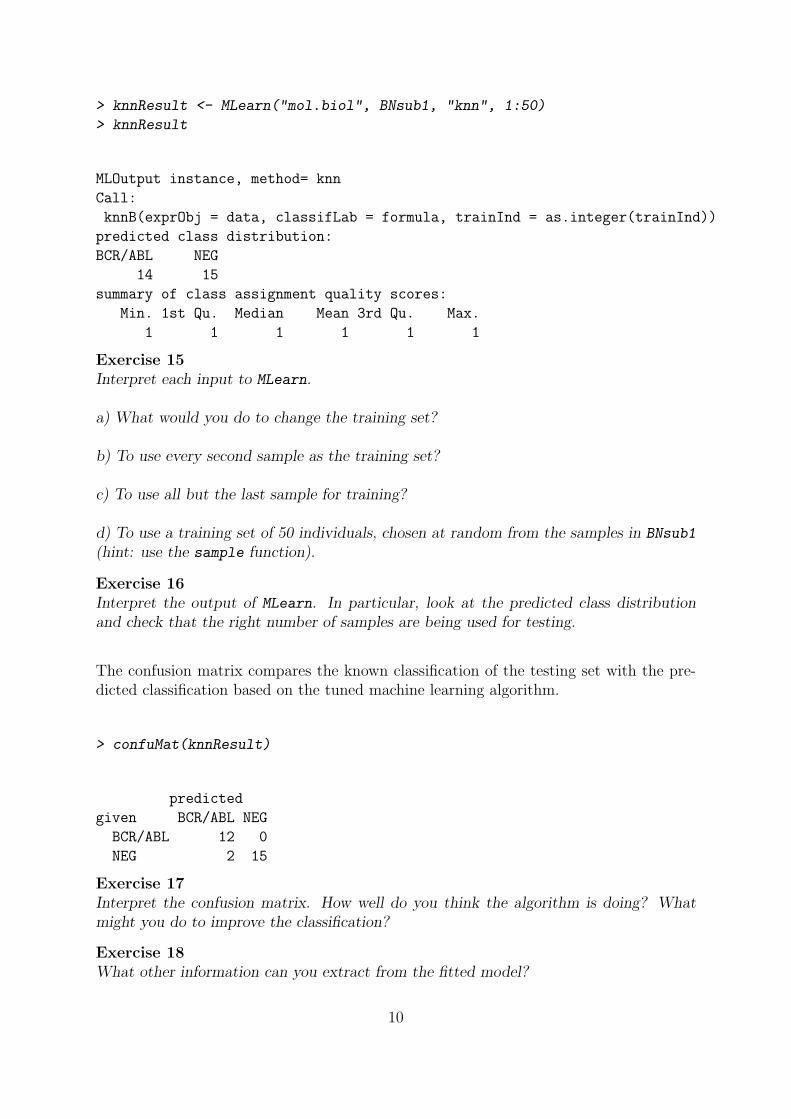
> knnResult <- MLearn("mol.biol", BNsub1, "knn", 1:50)

> knnResult

MLOutput instance, method= knn

Call:

knnB(exprObj = data, classifLab = formula, trainInd = as.integer(trainInd))

predicted class distribution:

BCR/ABL NEG

14 15

summary of class assignment quality scores:

Min. 1st Qu. Median Mean 3rd Qu. Max.

1 1 1 1 1 1

Exercise 15Interpret each input to MLearn.

a) What would you do to change the training set?

b) To use every second sample as the training set?

c) To use all but the last sample for training?

d) To use a training set of 50 individuals, chosen at random from the samples in BNsub1

(hint: use the sample function).

Exercise 16Interpret the output of MLearn. In particular, look at the predicted class distributionand check that the right number of samples are being used for testing.

The confusion matrix compares the known classification of the testing set with the pre-dicted classification based on the tuned machine learning algorithm.

> confuMat(knnResult)

predicted

given BCR/ABL NEG

BCR/ABL 12 0

NEG 2 15

Exercise 17Interpret the confusion matrix. How well do you think the algorithm is doing? Whatmight you do to improve the classification?

Exercise 18What other information can you extract from the fitted model?

10

Cross-validation

Cross-validation is often used to assess the prediction error of supervised machine learning.In order to get an accurate assessment it is important that all steps that can affect theoutcome are included in the cross-validation process.

In particular, the selection of features to use in the machine learning algorithm must beincluded within the cross-validation step.

The MLInterfaces package has a method for performing cross-validation. The methodis called xval. Ponder its help page (?xval) and think about how you might performcross-validation of BNsub1.

From the xval help page, it looks like we should be able to perform cross validation witha command like:

> knnXval <- xval(BNsub1, "mol.biol", knnB, xvalMethod = "LOO")

The first two arguments should be familiar. The third argument, knnB, specifies that wewill use the knn function. The final argument, xvalMethod , indicates the method thatwill be used for cross-validation. The cryptic ”LOO” stands for leave-one-out.

Exercise 19Describe in words the operation that xval is performing.

xval for leave-one-out cross-validation returns a list, with each element in the list beingthe result of a single cross validation.

Exercise 20What is the length of knnXval? Why?

Exercise 21Interpret the meaning of each element in knnXval.

Exercise 22What information is provided by the following command? How would you use this toassess the performance of this machine learning algorithm?

> table(given = BNsub1$mol.biol, predicted = knnXval)

predicted

given BCR/ABL NEG

BCR/ABL 35 2

NEG 2 40

11

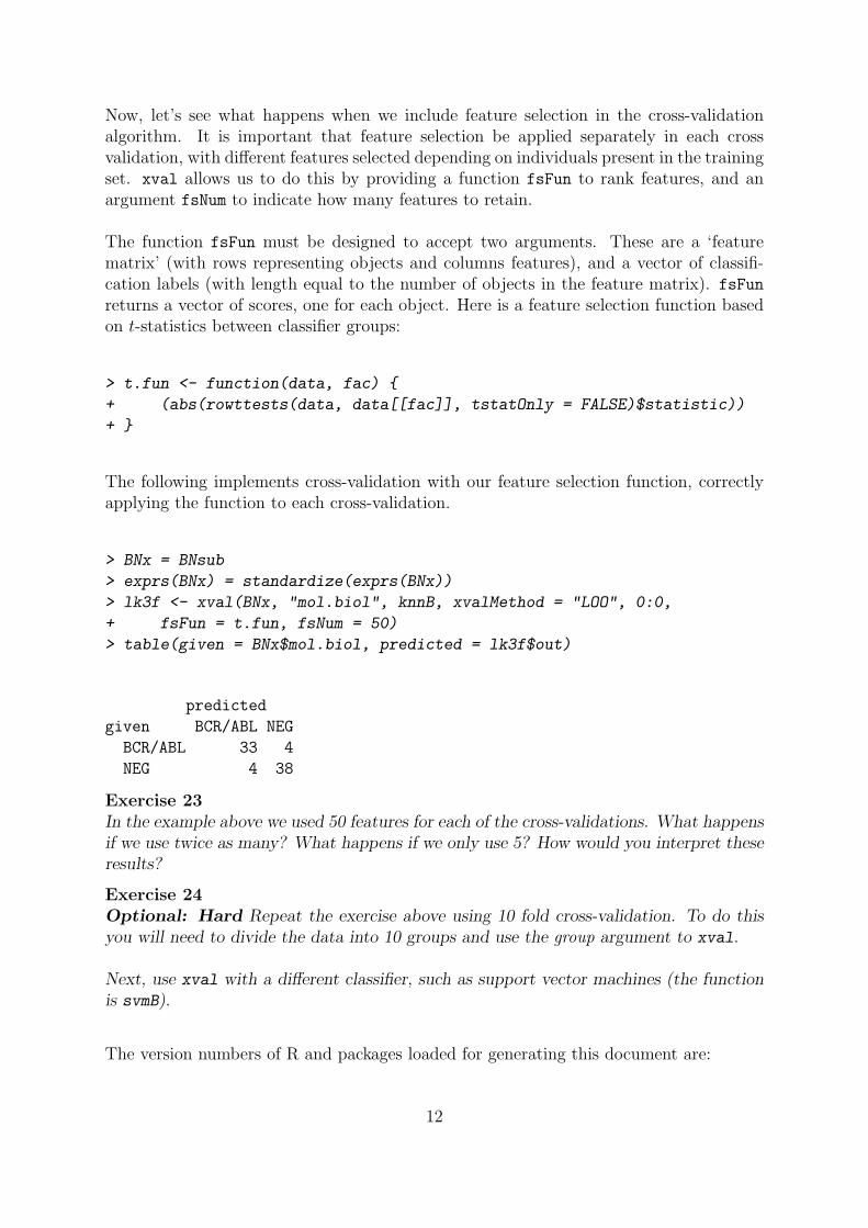
Now, let’s see what happens when we include feature selection in the cross-validationalgorithm. It is important that feature selection be applied separately in each crossvalidation, with different features selected depending on individuals present in the trainingset. xval allows us to do this by providing a function fsFun to rank features, and anargument fsNum to indicate how many features to retain.

The function fsFun must be designed to accept two arguments. These are a ‘featurematrix’ (with rows representing objects and columns features), and a vector of classifi-cation labels (with length equal to the number of objects in the feature matrix). fsFun

returns a vector of scores, one for each object. Here is a feature selection function basedon t-statistics between classifier groups:

> t.fun <- function(data, fac) {

+ (abs(rowttests(data, data[[fac]], tstatOnly = FALSE)$statistic))

+ }

The following implements cross-validation with our feature selection function, correctlyapplying the function to each cross-validation.

> BNx = BNsub

> exprs(BNx) = standardize(exprs(BNx))

> lk3f <- xval(BNx, "mol.biol", knnB, xvalMethod = "LOO", 0:0,

+ fsFun = t.fun, fsNum = 50)

> table(given = BNx$mol.biol, predicted = lk3f$out)

predicted

given BCR/ABL NEG

BCR/ABL 33 4

NEG 4 38

Exercise 23In the example above we used 50 features for each of the cross-validations. What happensif we use twice as many? What happens if we only use 5? How would you interpret theseresults?

Exercise 24Optional: Hard Repeat the exercise above using 10 fold cross-validation. To do thisyou will need to divide the data into 10 groups and use the group argument to xval.

Next, use xval with a different classifier, such as support vector machines (the functionis svmB).

The version numbers of R and packages loaded for generating this document are:

12

Version 2.3.1 Patched (2006-06-08 r38315)

powerpc-apple-darwin8.6.0

attached base packages:

[1] "splines" "tools" "methods" "stats" "graphics" "grDevices"

[7] "utils" "datasets" "base"

other attached packages:

MLInterfaces class genefilter survival RColorBrewer ALL

"1.4.0" "7.2-27.1" "1.10.1" "2.26" "0.2-3" "1.2.1"

Biobase

"1.10.0"

References

R. Gentleman, W. Huber, V. Carey, R. Irizarry, and S. Dudoit, editors. Bioinformaticsand Computational Biology Solutions Using R and Bioconductor. Springer, 2005.

L. Kaufman and P. J. Rousseeuw. Finding Groups in Data. Wiley, 1990.

13