1

An Investor’s Guide to the Risk Versus Return Conundrum: Isolating Critical Considerations, Identifying Measurement Challenges and Evaluating Alternative Approaches By Alan Snyderi, Joel Parrishii, Tuling Lamiii & Yunfei Zouiv

August 28, 2013

Abstract “A fool and his money are soon parted.” - Thomas Tusser, a 16th Century English Farmer No one wants to be the fool or even foolish in his investment management. In this article, we seek to make a contribution to each investor’s protective bulwark against these perils. Our goal is to create a framework for considering risk versus return tradeoffs that is both qualitative and quantitative. Too often, it has been a conundrum without a map, much less road signs along the way. We start with the investor; whether an individual or an institution, the issues are the same. Polonius in Shakespeare’s Hamlet provides sage advice paraphrased as: “To thine own self be true.” Be realistic and define risk tolerance, liquidity requirements (real and imagined), timeframes and return objectives. Accept that it is an iterative process with each criterion, including evaluating a single investment against a dynamically changing portfolio. Thus armed, we venture into the quicksand of data analysis, the boring but critical “how to.” Along the way we consider that past may not be prologue, e.g., our worst loss may be ahead of us. Being Chicken Little may be the healthiest approach to portfolio longevity. i Founder and Managing Partners of Shinnecock Partners, former CEO, Chairman and President of Answer Financial,

President of First Executive, CEO of Executive Life and Executive Vice President of Dean Witter (now Morgan Stanley), Harvard Business School Baker Scholar. ii Principal of Shinnecock Partners, former trader and analyst at First Executive, B.A. Columbia College. iii Analyst intern at Shinnecock Partners, MFE candidate in Financial Engineering at UCLA, former engineer at Edwards LifeSciences, M.S. UCLA, B.S. University of Illinois Urbana-Champaign. iv Quantitative analyst at Shinnecock Partners, Ph.D. candidate in Physics at UCLA, M.S. UCLA, awarded Chancellor’s Prize for outstanding academic merit, B.S. Zhejang University with Guanghua Scholarship. © 2013 Shinnecock Partners L.P. All rights reserved.

2

From here, Mark Twain’s often quoted “It’s not just the return on my capital but the return of my capital,” led us to review current risk and return measures with their concomitant strengths and weaknesses. Twain’s statement reflected his own substantial losses in the stock markets of his day (1835 – 1910). In this exploration, we note there is no single perfect risk/return measure that we could find. Nevertheless, we hope to shed some light on two measures not commonly used, which offer promise. The Omega Function is holistic, while the Pain Index dwells on the dark side of loss exposure. We decided that it would be a bridge too far to explore Monte Carlo simulations, data windowing and randomizing returns in this article. These approaches add complexity but offer additional depth and enhanced validity by extending many of the risk and return measures discussed herein. We will delve into them in future writings. Nassim Taleb offers counsel when he suggests that any money manager who undertakes his trade with no skin in the game, other than fees, is “fragile.” With his capital alongside the investor’s, he is robust. And best of all, with his capital and his soul on the line, he is “antifragile.”1 In closing, Will Rogers keeps all of us humble with his humor: “the quickest way to double your money is to fold it in half and put it in your pocket.” Of course, with billions to be managed, his advice only goes so far. Hence, read on… I. Historical Perspective The issue of risk versus return has tormented investors throughout time. Several historical examples highlight the challenge, provide current perspective and embody the adage that the misery of finding solutions is a shared experience. In 1602, the first stock exchange was founded in Amsterdam to solve an investment problem. At first, British, French and Dutch explorers raised capital by promising investors a percentage of their earnings (as much as 400%) or losses from individual voyages. While these ventures were often profitable, they were also extremely risky. Therefore, investors attempted to reduce their exposure by diversifying their investment across many different voyages. This eventually led to the establishment of the Dutch East India Companies, the first to sell company stock to the public via this new stock exchange.2 By investing in the company stock instead of specific voyages, investors found a way to spread their risk through the smoothing effects of diversification. Risk was disregarded during the Tulip Mania of 1634 - 1637. Tulip bulbs, introduced to Holland from Turkey, were already highly valued. But, following the discovery of a non-fatal plant virus which caused the petals to bloom in flames of contrasting colors, tulip bulb prices soared. As demand increased more quickly than supply, prices rose so fast that some were willing to trade their estates for hoped-for skyrocketing appreciation. In 1633 a farmhouse was sold for three rare tulip bulbs! Periodically during this craze, short

3

selling was banned, thwarting hedging. Ultimately, the government stepped in and annulled contracts with only a small payment to exit, compounding the risks (sadly, this history sounds almost familiar given some recent events). With pure speculation and few ways to control risk, this bubble burst as quickly as it inflated. People started to sell and a domino effect ensued. Tulip prices plummeted, creating panic across Holland. The take-away: unhedged speculation can result in devastating consequences!3,4 As financial markets developed in the nineteenth century, more sophisticated approaches began to emerge. Dow’s Theory, which was created by Charles Dow in the late 1800’s, and the Graham Theory of 1934, developed by Ben Graham, are two notable examples. Both methods were enabled by data, as new service providers collected information on stock and bond price movements, including underlying financial details. Dow laid the roots for technical analysis, using trend analysis to identify the direction of the market, summarized by his six basic tenets. 5 Graham’s Theory proposed that “risk comes from the overpricing of securities.” He emphasized the importance of maintaining a “margin of safety”6 by buying securities well below their conservative and/or liquidation value. Value investing was born, underpinned by a foundation of intense data analysis. However, Graham made a gross assumption that “true value” would buffer any downside exposure over time. Unconvinced that the markets could be predicted on a consistent basis, Alfred Winslow Jones devised a way to protect a fully invested portfolio from fickle market swings. He founded the first hedge fund in 1949 with starting capital of $100,000. Jones’s key insight was to create a conservative portfolio by combining two risky strategies, using leverage to buy shares of stocks and selling other shares short. Consequently, he developed the early concept of the hedge fund as a “well-hedged fund.” In the following years, Jones brought in other partners to manage portions of his firm’s capital, essentially creating the first “in-house fund of funds.” 7 Using this strategy, he outperformed many leading funds of the time and only experienced losses in two out of the 34 years.8 This remarkable performance proved that successful hedging can be achieved with robust tools to monitor risk and return. He diversified by position, portfolio manager (i.e., the human factor) and by being long as well as short. II. Critical Considerations Risk is the probability that an investment return will differ from its average historical return or compound annual growth rate (“CAGR”) and its future expected return, all during a defined investment period. Furthermore, there is both a risk of loss, as well as a risk of a potential gain over a particular time period. This variability can be statistically measured by the standard deviation (volatility) of the returns, the measure most typically used. The principle of risk and return is often seen as a “tradeoff” relationship, with the implication that increased returns require increased levels of risk. The probability of high profits subjects the investment to a greater chance of loss. This potential result leads the

4

investor to the challenge of the investment risk versus return conundrum. How can the “right” investment be determined?

The first step is to define the investment objective, specified mainly by the following factors: risk and return preference, time horizon, and liquidity requirements. In addition, an investor’s psychological profile must be ascertained: personality traits, values, lifestyle and his attitude towards money. For example, those who have gained wealth through inheritance tend to be risk averse because they may be unable to create new wealth from their own efforts, whereas successful entrepreneurs may be more optimistic and less risk-averse, because they feel that they are able to create new investment capital. Furthermore, an institutional decision-maker may be quite risk-averse as he seeks to balance current liability costs of a pension plan or other outflow requirement against the potential portfolio returns; he might also be acting to protect his own job and career prospects. Most organizations do not reward outsized positive performance versus the penalty exacted from losses. An investor’s desired time horizon for holding an investment often gives insight to risk tolerance. An investment with a short time horizon is more suitable for lower risk because there may not be sufficient time to recover from large losses. On the other hand, a longer time period may allow for large swings to be smoothed out in the pursuit of higher returns. If an investor demands a highly liquid investment, which can mean daily, monthly or quarterly liquidity, many alternatives can be quickly eliminated: most, if not all, private equity and venture capital, lockups requiring one- to five-year commitments, high first-year redemption or surrender charges, most direct ownership of real estate, etc. Traditionally, many less liquid assets offer attractive returns but demand intense scrutiny because once in, it may be impossible to leave without draconian haircuts to the returns and principal, if even possible at all. In sum, as liquidity constraints are loosened, potential returns may increase and underlying asset choices expand. Another gating dimension is how a single investment integrates into a total portfolio. The evaluation of one investment against alternatives must be combined with a determination of how well the chosen investment integrates into the whole. While a standalone investment may have attractive merit, it may not fit well with existing or anticipated holdings. Investing in an individual stock, asset, or strategy will expose the investor to risk that is only associated with that particular instrument. Consequently, this risk will be undiversified. Investing in an assortment of financial instruments or strategies offers several advantages. A multi-position portfolio can allow both diversification and “differsification” to be achieved, resulting in a reduction of overall investment risk and possibly higher returns. Diversification spreads investments across a variety of strategies, asset classes, markets, instruments traded, portfolio managers, geographic area, liquidity profiles, trade duration and so forth, to smooth out sector-specific risk. Differsification describes finding particular strategies or assets that will perform well under different economic conditions such as a volatile/stable market, economic inflation/deflation, and economic expansion/contraction9; in effect, one can create a portfolio for all economic seasons.1

5

A cornerstone of a well-diversified portfolio is low correlation. An ideal portfolio should include strategies with low correlations to one another. Correlation is the fractional amount by which one variable moves in relation to another. Correlation will be positive if the movement is in the same direction and negative if it is in the opposite direction. Its equation is:

where xi and yi represent two return series, and ∑ represents the sum. The two most commonly used correlations are Pearson’s correlation and Spearman’s rank correlation. Pearson’s correlation, calculated using the equation above, is best for continuous and normally distributed data. For distributions with significant departures from normality, Pearson’s correlation loses much of its applicability. Spearman’s rank correlation is the Pearson correlation coefficient between the ranked variables. Instead of calculating the correlation directly, it ranks the returns first, and then computes the Pearson’s correlation between the ranked series. Spearman's rank correlation is appropriate for both continuous and discrete variables with an implied linear relationship, and has no requirement for how the data should be distributed (i.e., does not assume a normal distribution). For much of this discussion on correlation, diversification and differsification, there is a critical caveat. With accurate insight, near-perfect predictions and an ability to wager it all on these talents, a non-diversified, non-differsified and correlated portfolio will outperform all others. However, the risk is very high if the insight is cloudy, the predictions wrong or timing askew. Such “bet the ranch” approaches are not for the faint of heart and have generally not been successful long-term strategies.

Autocorrelation can also play an important role in the analysis of investment return performance. Often called “lagged correlation” or “serial correlation,” autocorrelation is the correlation of a return series with itself over successive intervals of time. A positive autocorrelation indicates a high probability that a positive variation from the mean will be followed by another positive, or a negative variation from the mean will be followed by another negative. If an asset or strategy exhibits positive autocorrelation historically, and its return is observed to be positive over recent time intervals, it will have a tendency to have a positive return in the next period. On the other hand, if there has been positive autocorrelation historically, but the return is observed to be negative over recent time periods, it will have a tendency to exhibit a negative return in the next period. A negative autocorrelation indicates a higher probability that a positive variation from the mean will be followed by a negative or vice versa.10

6

III. Measurement Challenges While one of the most imperative challenges an investor faces is determining how well an investment is performing, several obstacles may arise when analyzing returns.

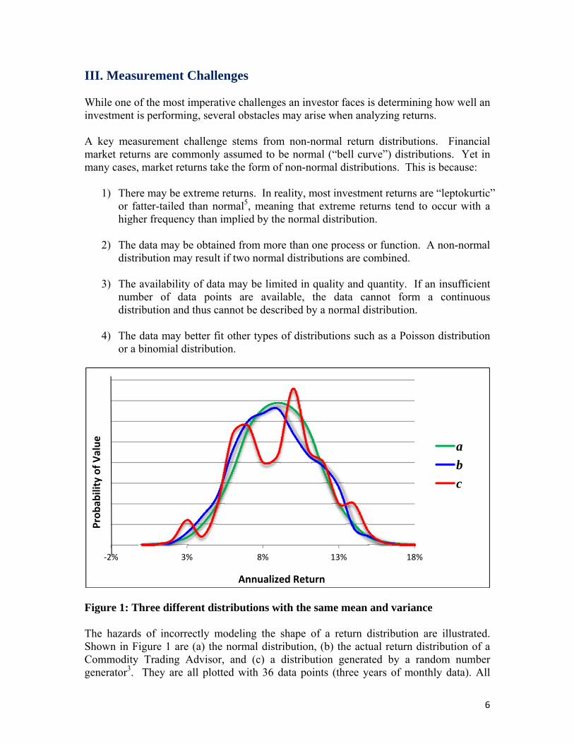
A key measurement challenge stems from non-normal return distributions. Financial market returns are commonly assumed to be normal (“bell curve”) distributions. Yet in many cases, market returns take the form of non-normal distributions. This is because:

1) There may be extreme returns. In reality, most investment returns are “leptokurtic” or fatter-tailed than normal5, meaning that extreme returns tend to occur with a higher frequency than implied by the normal distribution.

2) The data may be obtained from more than one process or function. A non-normal distribution may result if two normal distributions are combined.

3) The availability of data may be limited in quality and quantity. If an insufficient number of data points are available, the data cannot form a continuous distribution and thus cannot be described by a normal distribution.

4) The data may better fit other types of distributions such as a Poisson distribution or a binomial distribution.

Figure 1: Three different distributions with the same mean and variance The hazards of incorrectly modeling the shape of a return distribution are illustrated. Shown in Figure 1 are (a) the normal distribution, (b) the actual return distribution of a Commodity Trading Advisor, and (c) a distribution generated by a random number generator3. They are all plotted with 36 data points (three years of monthly data). All

‐2% 3% 8% 13% 18%

a

b

c

Annualized Return

Probab

ility of Value

7

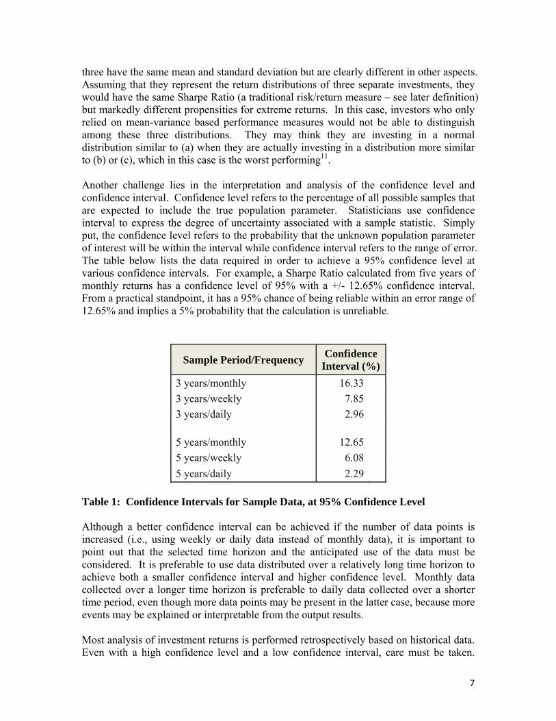
three have the same mean and standard deviation but are clearly different in other aspects. Assuming that they represent the return distributions of three separate investments, they would have the same Sharpe Ratio (a traditional risk/return measure – see later definition) but markedly different propensities for extreme returns. In this case, investors who only relied on mean-variance based performance measures would not be able to distinguish among these three distributions. They may think they are investing in a normal distribution similar to (a) when they are actually investing in a distribution more similar to (b) or (c), which in this case is the worst performing11. Another challenge lies in the interpretation and analysis of the confidence level and confidence interval. Confidence level refers to the percentage of all possible samples that are expected to include the true population parameter. Statisticians use confidence interval to express the degree of uncertainty associated with a sample statistic. Simply put, the confidence level refers to the probability that the unknown population parameter of interest will be within the interval while confidence interval refers to the range of error. The table below lists the data required in order to achieve a 95% confidence level at various confidence intervals. For example, a Sharpe Ratio calculated from five years of monthly returns has a confidence level of 95% with a +/- 12.65% confidence interval. From a practical standpoint, it has a 95% chance of being reliable within an error range of 12.65% and implies a 5% probability that the calculation is unreliable.

Sample Period/Frequency Confidence

Interval (%)

3 years/monthly 16.33

3 years/weekly 7.85

3 years/daily 2.96

5 years/monthly 12.65

5 years/weekly 6.08

5 years/daily 2.29

Table 1: Confidence Intervals for Sample Data, at 95% Confidence Level Although a better confidence interval can be achieved if the number of data points is increased (i.e., using weekly or daily data instead of monthly data), it is important to point out that the selected time horizon and the anticipated use of the data must be considered. It is preferable to use data distributed over a relatively long time horizon to achieve both a smaller confidence interval and higher confidence level. Monthly data collected over a longer time horizon is preferable to daily data collected over a shorter time period, even though more data points may be present in the latter case, because more events may be explained or interpretable from the output results.

Most analysis of investment returns is performed retrospectively based on historical data. Even with a high confidence level and a low confidence interval, care must be taken.

8

Does the sampled period accurately reflect all of the events that could happen in the future? Past may not be prologue. While useful information is learned and intelligence secured, this point must be factored into the evaluation. Determining the most relevant sample period is further confounded by an assessment of:

1. Autocorrelation – will the current pattern persist, arguing for a greater weighting of more current experience?

2. Strategy implementation - strategies may have morphed over time. Has the implementation been consistently applied over the entire data sample?

In 2008, many large institutions relied on Value at Risk (“VAR”) techniques with relatively short look-back periods, i.e., heavily weighted to recent data (also, many VAR models relied on mean-variance analysis, with all its shortcomings). Unfortunately, this approach woefully underestimated tail risk and the size of potential drawdowns. Alas, there is no perfect approach or simple solution. Judgment based on multiple scenario analysis may be the best answer. Returning to the issue of a single investment versus portfolio level determination, all of these variables blend into the proverbial Gordian Knot. How often has rebalancing occurred or even should occur? For example, there is the friction of transaction costs and slippage, underlying liquidity constraints, minimum investment requirements, etc. Each must be evaluated in this delicate balancing act – more tradeoffs! IV. Criteria for Evaluation Although most financial analysts agree that no single measurement can give a complete understanding of an investment’s performance, it is important to identify which ones might be most effective. We believe a good risk/return measure must exhibit as many of the following characteristics as possible:

1. Realistic: Not rely on assumptions that all data behave according to theoretical distributions. It must be applicable to data in the real world.

2. Practical and Implementable: Not be overly complex, time intensive or costly to implement or produce. It should be well understood by those who will use it, e.g., an understanding of its imperfections.

3. Predictive: Forecast the future.

4. Objective-centric: Take the desired risk and return preference of the investor into consideration. It should match the investor’s time horizon.

5. Suitable for imperfect data: Be able to draw some conclusions at a high confidence level with a limited amount of information and to work with other data imperfections, such as non-continuous (discrete) data and high volatility.

9

6. Define worst drawdown: Capture the worst possible loss an investor is willing to

tolerate to accomplish his desired return.

7. Differentiate between upside/downside volatility: Ideally, each should be measured independently.

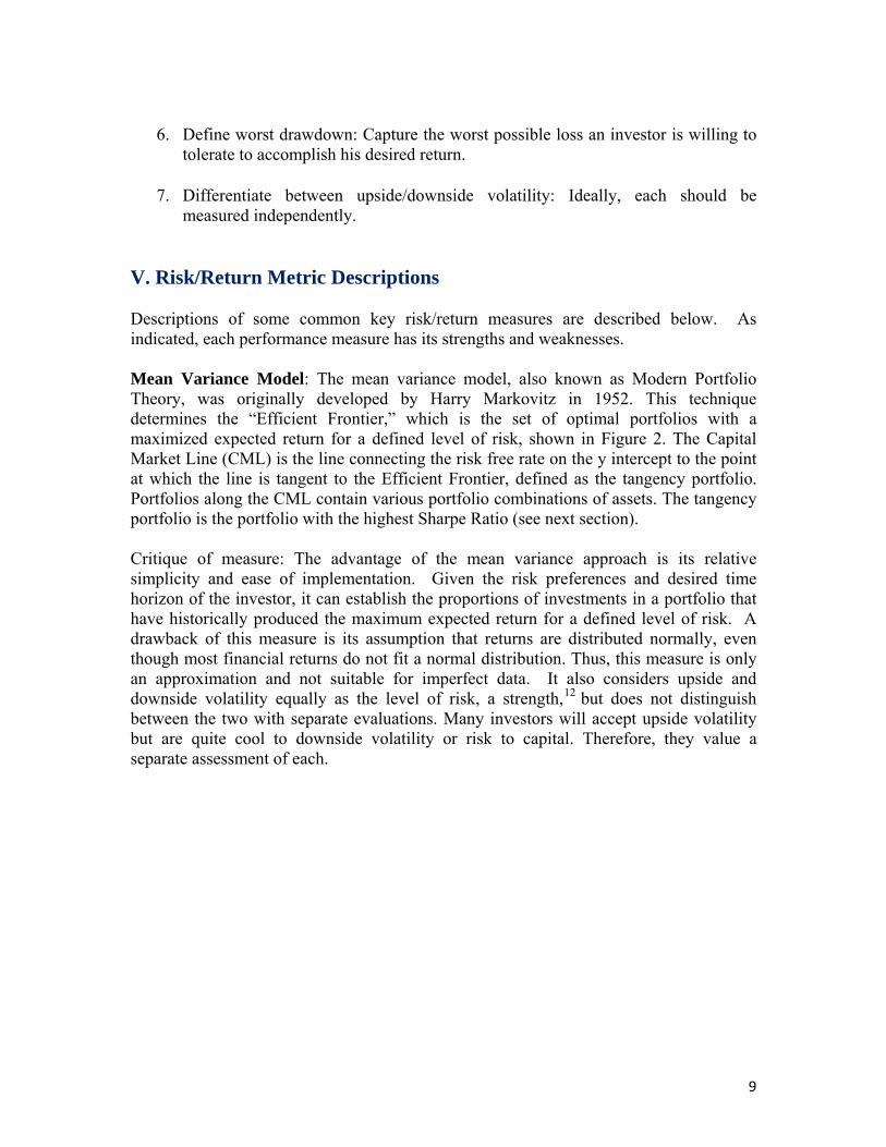
V. Risk/Return Metric Descriptions Descriptions of some common key risk/return measures are described below. As indicated, each performance measure has its strengths and weaknesses. Mean Variance Model: The mean variance model, also known as Modern Portfolio Theory, was originally developed by Harry Markovitz in 1952. This technique determines the “Efficient Frontier,” which is the set of optimal portfolios with a maximized expected return for a defined level of risk, shown in Figure 2. The Capital Market Line (CML) is the line connecting the risk free rate on the y intercept to the point at which the line is tangent to the Efficient Frontier, defined as the tangency portfolio. Portfolios along the CML contain various portfolio combinations of assets. The tangency portfolio is the portfolio with the highest Sharpe Ratio (see next section). Critique of measure: The advantage of the mean variance approach is its relative simplicity and ease of implementation. Given the risk preferences and desired time horizon of the investor, it can establish the proportions of investments in a portfolio that have historically produced the maximum expected return for a defined level of risk. A drawback of this measure is its assumption that returns are distributed normally, even though most financial returns do not fit a normal distribution. Thus, this measure is only an approximation and not suitable for imperfect data. It also considers upside and downside volatility equally as the level of risk, a strength,12 but does not distinguish between the two with separate evaluations. Many investors will accept upside volatility but are quite cool to downside volatility or risk to capital. Therefore, they value a separate assessment of each.

10

Figure 2: Diagram depicting the Efficient Frontier Sharpe Ratio: Invented by William Sharpe in 1966, the Sharpe Ratio is defined as the annual return of an investment above the risk free rate, also called the excess return, divided by the volatility of the return. In short, it is a measure of “reward per unit of risk.”

Sharpe Ratio = σ

where R is the return, Rf is the risk free rate and σ is the volatility

Critique of measure: The Sharpe Ratio quantifies the risk/return trade-off and how well the return compensates the investor for the risk taken. Its predicate is the mean variance model, giving it similar weaknesses. And, as a single number, little is learned about the consistency of returns. Sortino Ratio: The Sortino Ratio is the annual return above the risk free rate divided by downside volatility, or the “reward per unit of downside volatility.” The ratio was named after Frank Sortino, an early pioneer in downside risk optimization, but was developed by Brian Rorn in 1983. It modified the Sharpe Ratio by separating downside volatility from upside volatility. Downside volatility is variation below a target rate of return while upside volatility is variation above the target.

Sortino Ratio = σ

where R is the return, Rf is the risk free rate and σ is the volatility

Critique of measure: The Sortino Ratio focuses on what many investors fear most, capital loss. It quantifies the risk/return trade-off, describing how well the return compensates the investor per unit of downside risk. However, it does not account for the fact that most returns are non-normally distributed.

11

Maximum Drawdown: Maximum Drawdown is the single largest loss experienced (biggest drop from peak to trough) over a defined time period. Critique of measure: The Maximum Drawdown is a useful measure for evaluating an investment because it can be used to evaluate the maximum loss an investor is willing to tolerate. However, it cannot be utilized as a stand-alone metric since it only accounts for the worst loss without regard to frequency or duration. Calmar Ratio: The Calmar Ratio, also known as the drawdown ratio, was created by Terry Young in 1991. It is the 36-month average annual return above the risk free rate, divided by the maximum drawdown over 36 months.

Calmar Ratio =

where R is the return and Rf is the risk free rate

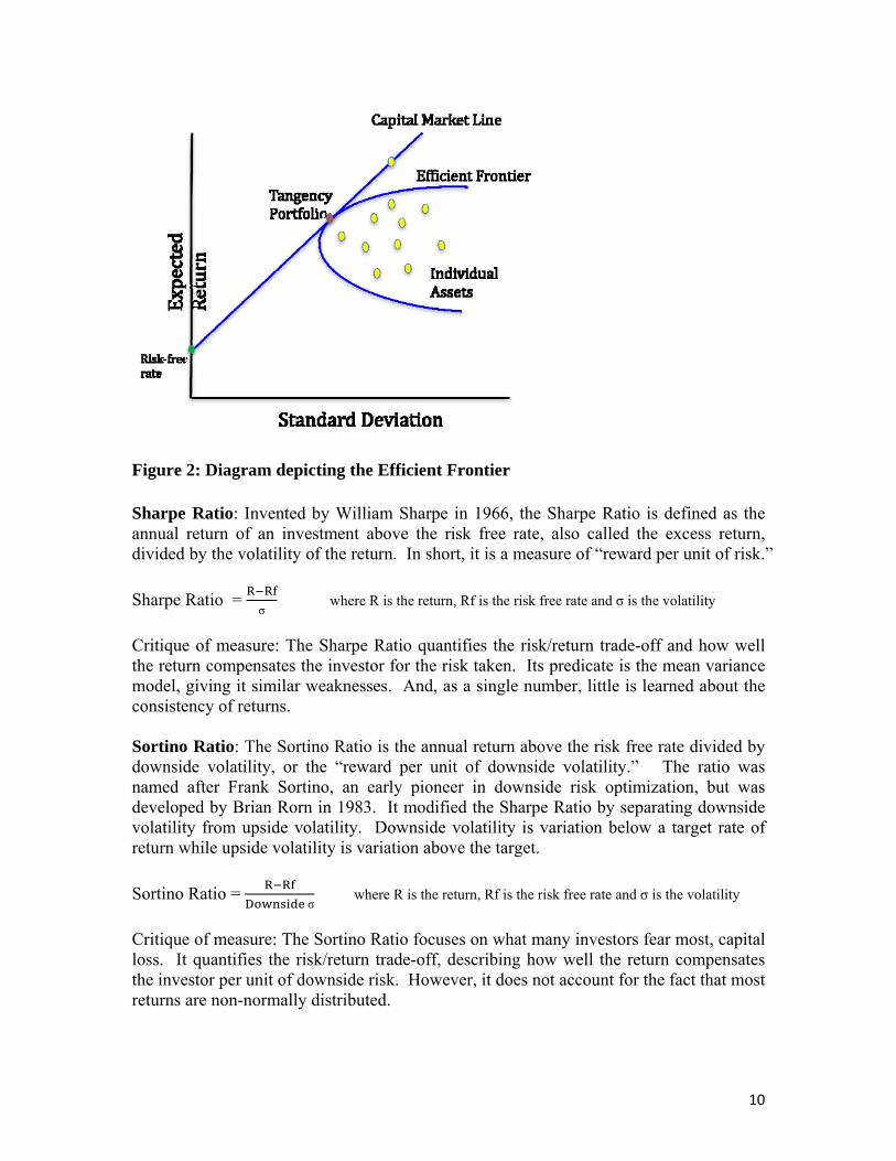
Critique of measure: The Calmar Ratio puts the maximum drawdown in a risk/return tradeoff context. In effect, the investor sees how much return might be realized if he is willing to absorb a certain amount of risk. It differentiates between upside and downside volatility, but only addresses the downside portion for the defined time period. It also assumes a normal distribution, and therefore results in an approximation. Martin Ratio: The Martin Ratio was created by Peter Martin in 1987 and is the annual return above the risk free rate, divided by the Ulcer Index. The Ulcer Index measures the depth and duration of all drawdowns from each earlier high in price in a given period. It essentially measures the “severity of drawdowns,” or the extent of loss that each drawdown incurs.13

Ulcer Index =⋯

where R 100

and N is the total number of data points, monthly or weekly.

Martin Ratio =

where R is the return and Rf is the risk free rate

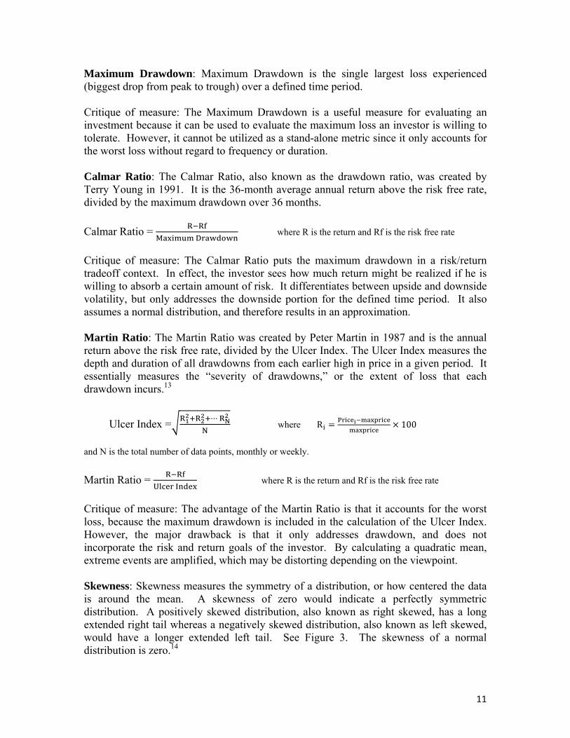
Critique of measure: The advantage of the Martin Ratio is that it accounts for the worst loss, because the maximum drawdown is included in the calculation of the Ulcer Index. However, the major drawback is that it only addresses drawdown, and does not incorporate the risk and return goals of the investor. By calculating a quadratic mean, extreme events are amplified, which may be distorting depending on the viewpoint. Skewness: Skewness measures the symmetry of a distribution, or how centered the data is around the mean. A skewness of zero would indicate a perfectly symmetric distribution. A positively skewed distribution, also known as right skewed, has a long extended right tail whereas a negatively skewed distribution, also known as left skewed, would have a longer extended left tail. See Figure 3. The skewness of a normal distribution is zero.14

12

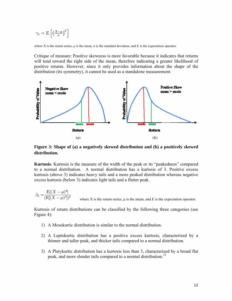
where X is the return series, μ is the mean, σ is the standard deviation, and E is the expectation operator.

Critique of measure: Positive skewness is more favorable because it indicates that returns will tend toward the right side of the mean, therefore indicating a greater likelihood of positive returns. However, since it only provides information about the shape of the distribution (its symmetry), it cannot be used as a standalone measurement.

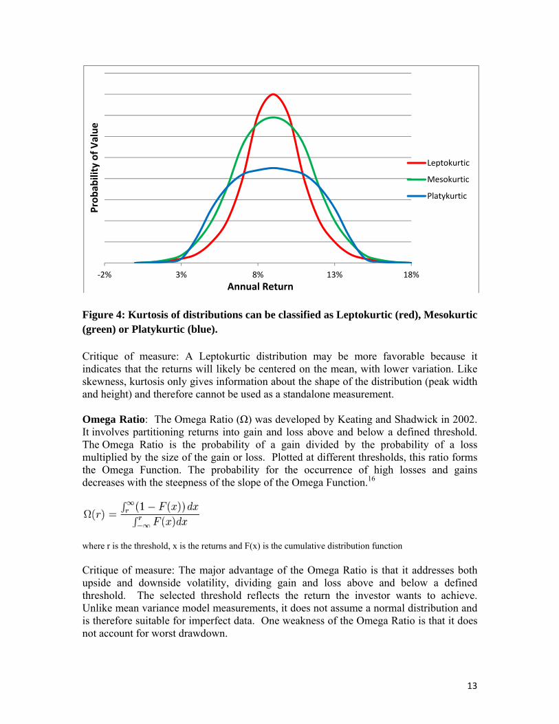
Figure 3: Shape of (a) a negatively skewed distribution and (b) a positively skewed distribution. Kurtosis: Kurtosis is the measure of the width of the peak or its “peakedness” compared to a normal distribution. A normal distribution has a kurtosis of 3. Positive excess kurtosis (above 3) indicates heavy tails and a more peaked distribution whereas negative excess kurtosis (below 3) indicates light tails and a flatter peak.

where X is the return series, μ is the mean, and E is the expectation operator. Kurtosis of return distributions can be classified by the following three categories (see Figure 4):

1) A Mesokurtic distribution is similar to the normal distribution.

2) A Leptokurtic distribution has a positive excess kurtosis, characterized by a thinner and taller peak, and thicker tails compared to a normal distribution.

3) A Platykurtic distribution has a kurtosis less than 3, characterized by a broad flat

peak, and more slender tails compared to a normal distribution.15

(a) (b)

13

Figure 4: Kurtosis of distributions can be classified as Leptokurtic (red), Mesokurtic (green) or Platykurtic (blue). Critique of measure: A Leptokurtic distribution may be more favorable because it indicates that the returns will likely be centered on the mean, with lower variation. Like skewness, kurtosis only gives information about the shape of the distribution (peak width and height) and therefore cannot be used as a standalone measurement. Omega Ratio: The Omega Ratio (Ω) was developed by Keating and Shadwick in 2002. It involves partitioning returns into gain and loss above and below a defined threshold. The Omega Ratio is the probability of a gain divided by the probability of a loss multiplied by the size of the gain or loss. Plotted at different thresholds, this ratio forms the Omega Function. The probability for the occurrence of high losses and gains decreases with the steepness of the slope of the Omega Function.16

where r is the threshold, x is the returns and F(x) is the cumulative distribution function Critique of measure: The major advantage of the Omega Ratio is that it addresses both upside and downside volatility, dividing gain and loss above and below a defined threshold. The selected threshold reflects the return the investor wants to achieve. Unlike mean variance model measurements, it does not assume a normal distribution and is therefore suitable for imperfect data. One weakness of the Omega Ratio is that it does not account for worst drawdown.

‐2% 3% 8% 13% 18%

Leptokurtic

Mesokurtic

Platykurtic

Annual Return

Probab

ility of Value

14

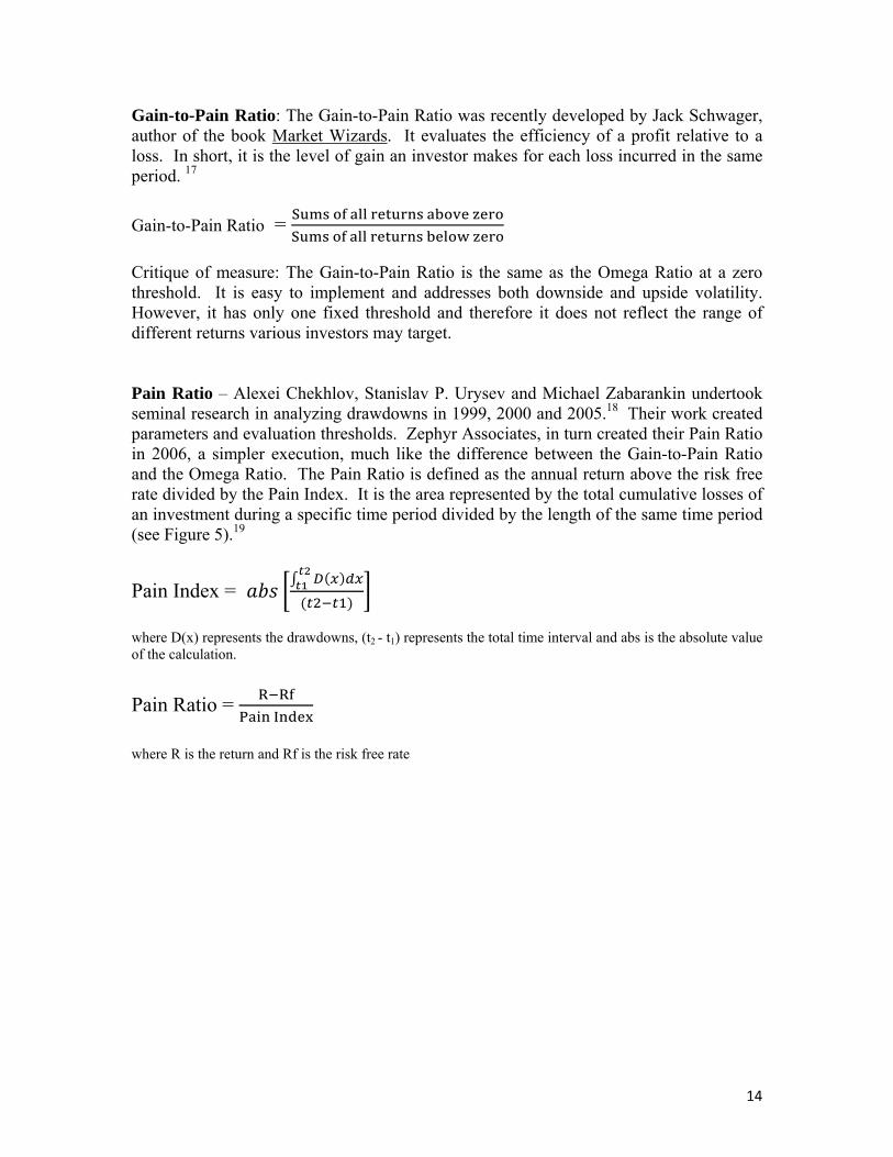
Gain-to-Pain Ratio: The Gain-to-Pain Ratio was recently developed by Jack Schwager, author of the book Market Wizards. It evaluates the efficiency of a profit relative to a loss. In short, it is the level of gain an investor makes for each loss incurred in the same period. 17

Gain-to-Pain Ratio =

Critique of measure: The Gain-to-Pain Ratio is the same as the Omega Ratio at a zero threshold. It is easy to implement and addresses both downside and upside volatility. However, it has only one fixed threshold and therefore it does not reflect the range of different returns various investors may target. Pain Ratio – Alexei Chekhlov, Stanislav P. Urysev and Michael Zabarankin undertook seminal research in analyzing drawdowns in 1999, 2000 and 2005.18 Their work created parameters and evaluation thresholds. Zephyr Associates, in turn created their Pain Ratio in 2006, a simpler execution, much like the difference between the Gain-to-Pain Ratio and the Omega Ratio. The Pain Ratio is defined as the annual return above the risk free rate divided by the Pain Index. It is the area represented by the total cumulative losses of an investment during a specific time period divided by the length of the same time period (see Figure 5).19

Pain Index = where D(x) represents the drawdowns, (t2 - t1) represents the total time interval and abs is the absolute value of the calculation.

Pain Ratio =

where R is the return and Rf is the risk free rate

15

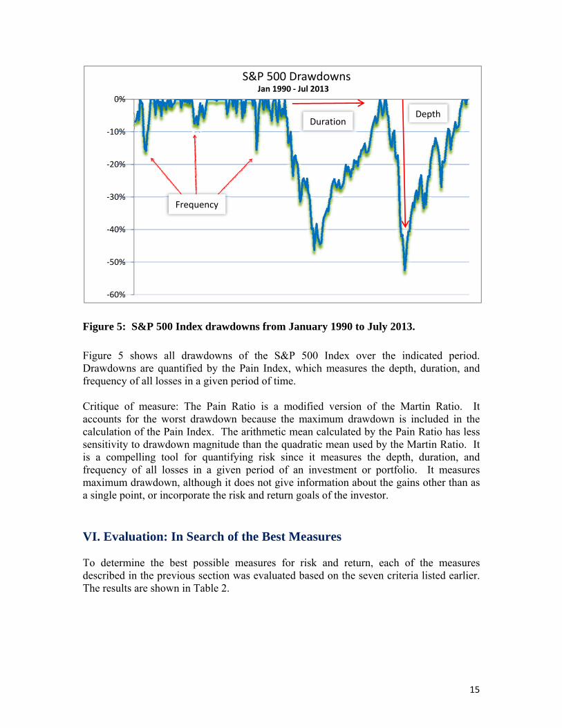
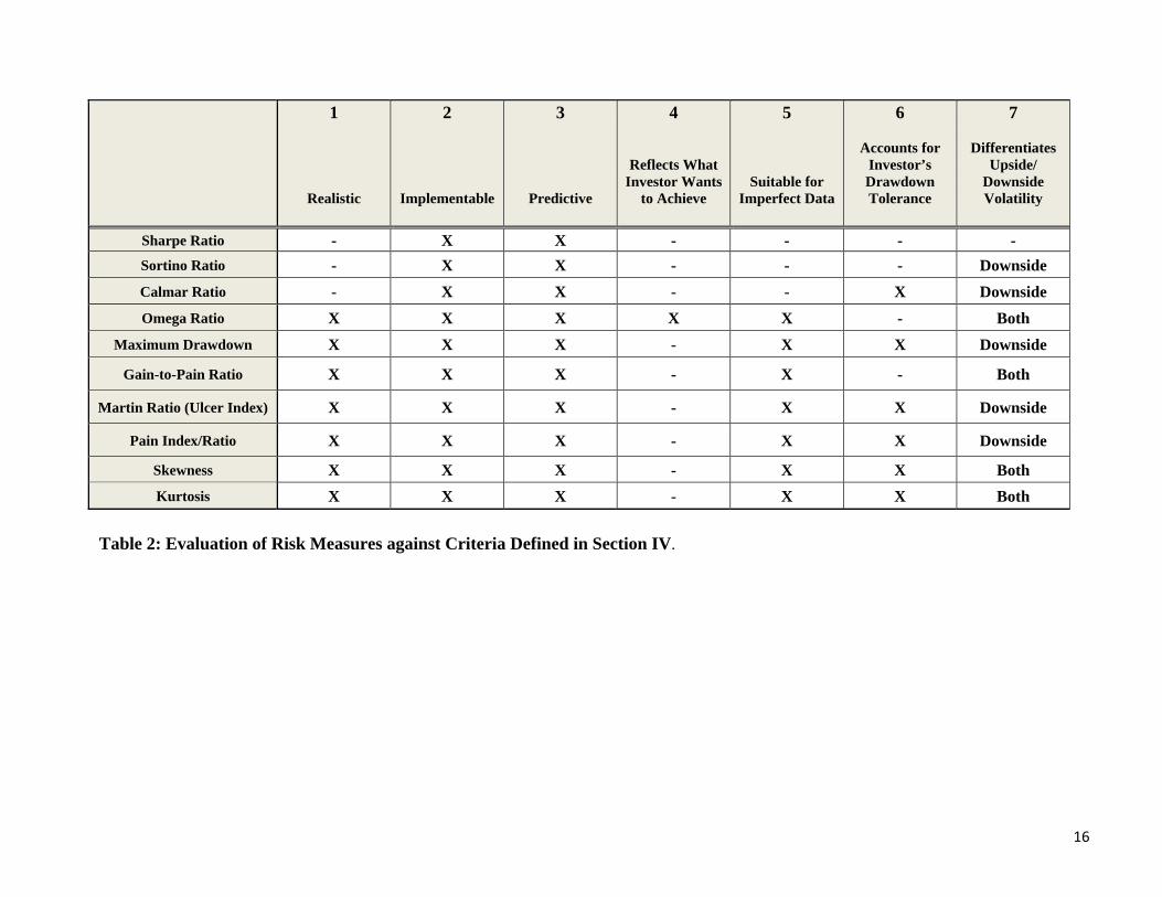
Figure 5: S&P 500 Index drawdowns from January 1990 to July 2013. Figure 5 shows all drawdowns of the S&P 500 Index over the indicated period. Drawdowns are quantified by the Pain Index, which measures the depth, duration, and frequency of all losses in a given period of time. Critique of measure: The Pain Ratio is a modified version of the Martin Ratio. It accounts for the worst drawdown because the maximum drawdown is included in the calculation of the Pain Index. The arithmetic mean calculated by the Pain Ratio has less sensitivity to drawdown magnitude than the quadratic mean used by the Martin Ratio. It is a compelling tool for quantifying risk since it measures the depth, duration, and frequency of all losses in a given period of an investment or portfolio. It measures maximum drawdown, although it does not give information about the gains other than as a single point, or incorporate the risk and return goals of the investor. VI. Evaluation: In Search of the Best Measures To determine the best possible measures for risk and return, each of the measures described in the previous section was evaluated based on the seven criteria listed earlier. The results are shown in Table 2.

‐60%

‐50%

‐40%

‐30%

‐20%

‐10%

0%

S&P 500 DrawdownsJan 1990 ‐ Jul 2013

Frequency

DurationDepth

16

1

Realistic

2

Implementable

3

Predictive

4

Reflects What Investor Wants

to Achieve

5

Suitable for Imperfect Data

6

Accounts for Investor’s Drawdown Tolerance

7

Differentiates Upside/

Downside Volatility

Sharpe Ratio - X X - - - -

Sortino Ratio - X X - - - Downside

Calmar Ratio - X X - - X Downside

Omega Ratio X X X X X - Both

Maximum Drawdown X X X - X X Downside

Gain-to-Pain Ratio X X X - X - Both

Martin Ratio (Ulcer Index) X X X - X X Downside

Pain Index/Ratio X X X - X X Downside

Skewness X X X - X X Both

Kurtosis X X X - X X Both

Table 2: Evaluation of Risk Measures against Criteria Defined in Section IV.

17

Although each of the listed measures meets some of the criteria, we can observe that the Omega Ratio satisfies most of the criteria except for the threshold for worst drawdown. The Omega Function, a plot of Omega Ratios at different thresholds, measures the risk of an investment asset or portfolio, incorporating all of the information from historical returns within a distribution. Unlike many commonly used measures, it does not assume that returns take the form of a normal distribution. It accounts for both upside and downside volatility by partitioning a probability of a gain above a threshold and a probability of a loss below a threshold. This threshold is selected based on the investor’s risk preferences. It is an attractive risk/return measure because it is also relatively simple to use and implement. The Pain Index/Ratio also satisfy many of the criteria. These quantitatively measure the depth, duration, and frequency of all losses in a given period. The Pain Index is a particularly useful companion to the Omega Function due to its focus on losses, and it delivers a more complete picture than Maximum Drawdown and the Martin Ratio. A closer look at the Omega and Pain Index/Ratio will show how they can be used together to give a well-rounded interpretation of investment performance. VII. A Deeper Interpretation of the Omega Ratio The Omega Ratio, a “universal” performance measure, involves partitioning returns into loss and gain above and below a given threshold. In many respects, Omega can be thought of as a payoff function. The higher the Omega Ratio, the better.20 Its limitations are discussed in Part VIII. When Omega Ratios are plotted at different thresholds, this forms the Omega Function, which has two significant advantages over traditional measures:

It is designed to incorporate all of the information about the risk and return of a portfolio within its return distribution. It incorporates the analysis of higher momentsv – i.e., skew, kurtosis.

Its precise value is directly determined by an individual investor’s risk appetite.

In contrast to the Sharpe Ratio, where only the first two moments (mean, variance) have an influence on the risk measure, the Omega Ratio takes into account all moments of the distribution. Risk information is encoded in the slope of the Omega Function: generally, the steeper the slope, the less likely extreme returns will occur.21

v In statistics, “moment” is defined as the expected value of the product formed by multiplying together a

set of one or more variables, each to a specified power.

18

In practice, Omega will sometimes show very different rankings of an investment asset or portfolio than those derived using the Sharpe Ratio, Sortino Ratio or Mean-Variance.22

If the shape of the return distribution is similar to a normal distribution, it agrees with traditional measures. But if the return distribution differs significantly from the normal bell curve, it provides crucial adjustments to these simpler traditional approximations.23

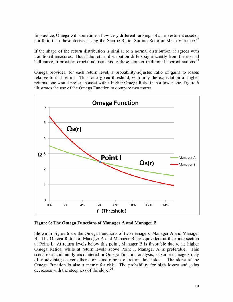
Omega provides, for each return level, a probability-adjusted ratio of gains to losses relative to that return. Thus, at a given threshold, with only the expectation of higher returns, one would prefer an asset with a higher Omega Ratio than a lower one. Figure 6 illustrates the use of the Omega Function to compare two assets.

Figure 6: The Omega Functions of Manager A and Manager B. Shown in Figure 6 are the Omega Functions of two managers, Manager A and Manager B. The Omega Ratios of Manager A and Manager B are equivalent at their intersection at Point I. At return levels below this point, Manager B is favorable due to its higher Omega Ratios, while at return levels above Point I, Manager A is preferable. This scenario is commonly encountered in Omega Function analysis, as some managers may offer advantages over others for some ranges of return thresholds. The slope of the Omega Function is also a metric for risk. The probability for high losses and gains decreases with the steepness of the slope.24

0

1

2

3

4

5

6

0% 2% 4% 6% 8% 10% 12% 14%

Ω

r (Threshold)

Omega Function

Manager A

Manager B

ΩB(r)

ΩA(r)Point I

19

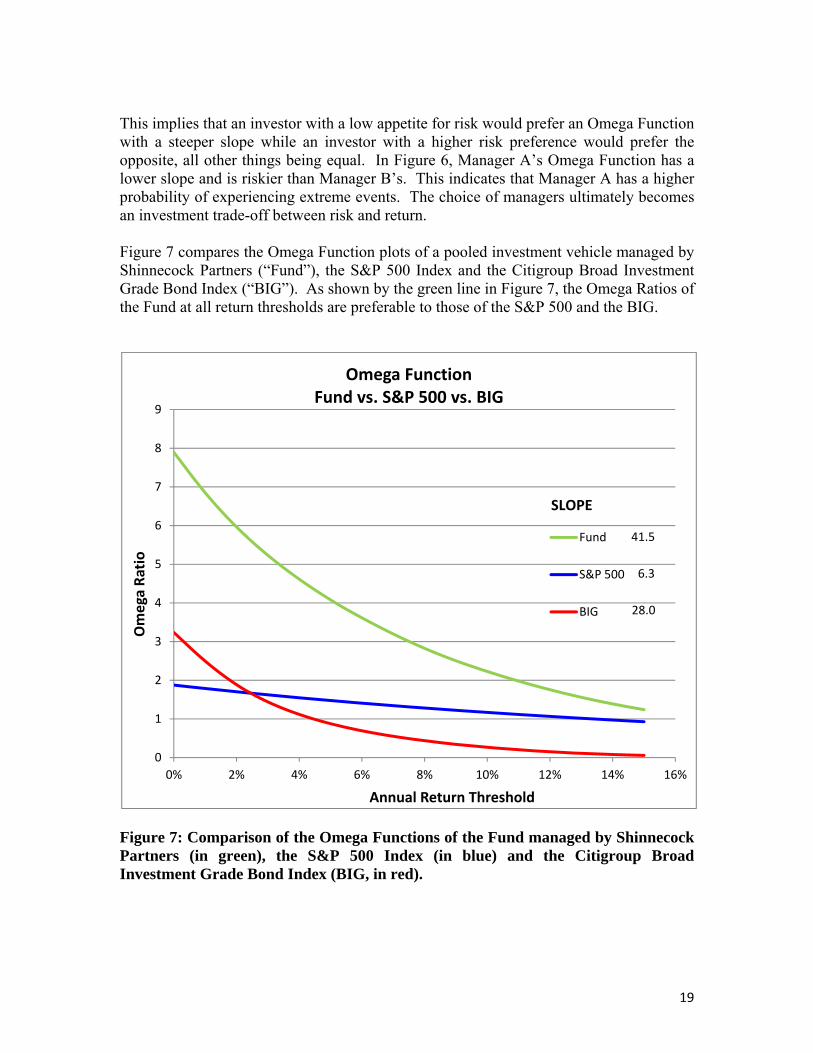
This implies that an investor with a low appetite for risk would prefer an Omega Function with a steeper slope while an investor with a higher risk preference would prefer the opposite, all other things being equal. In Figure 6, Manager A’s Omega Function has a lower slope and is riskier than Manager B’s. This indicates that Manager A has a higher probability of experiencing extreme events. The choice of managers ultimately becomes an investment trade-off between risk and return. Figure 7 compares the Omega Function plots of a pooled investment vehicle managed by Shinnecock Partners (“Fund”), the S&P 500 Index and the Citigroup Broad Investment Grade Bond Index (“BIG”). As shown by the green line in Figure 7, the Omega Ratios of the Fund at all return thresholds are preferable to those of the S&P 500 and the BIG.

Figure 7: Comparison of the Omega Functions of the Fund managed by Shinnecock Partners (in green), the S&P 500 Index (in blue) and the Citigroup Broad Investment Grade Bond Index (BIG, in red).

0

1

2

3

4

5

6

7

8

9

0% 2% 4% 6% 8% 10% 12% 14% 16%

Omega Ratio

Annual Return Threshold

Omega FunctionFund vs. S&P 500 vs. BIG

Fund

S&P 500

BIG

41.5

6.3

28.0

SLOPE

20

VIII. No Single Measurement Can be the Perfect One Although Omega captures an abundant amount of information, it has several drawbacks. One drawback is that it is leverage biased, which means that for investment assets that have a higher proportion (in frequency and magnitude) of returns over a given threshold, the Omega Ratio of those assets is increased by leveraging them.25 When returns are leveraged, both the “win” portion (numerator) and the “loss” portion (denominator) will increase in magnitude, but the win portion will increase by a greater proportion. If we only consider the Omega Ratio of a manager, we would always prefer, for example, the “3X” version of a money manager to the unleveraged version of the same manager at the threshold range shown in Figure 8.

Figure 8: Omega Functions of a Manager at 1X leverage (green) and 3X leverage (red). Figure 8 plots the Omega Ratios of an actual hedge fund manager at both standard and “3X” leverage. Observe that while the Omega Ratio of the leveraged vehicle is higher than the unleveraged vehicle at all thresholds shown, the flatter slope of the “3X” version is indicative of greater relative risk. Therefore, the Omega Function plot should always be evaluated in comparative analysis.

0

0.5

1

1.5

2

2.5

0% 2% 4% 6% 8% 10% 12% 14% 16%

Omega Function

ManagerA_1X

ManagerA_3X

Ω

r (Threshold)

ΩA_3X(r)

ΩA_1X(r)

21

The maximum decline that an investment has experienced, from “peak” to “trough,” i.e., “peak-to-valley drawdown,” is not clearly evident in the Omega Function, another drawback. A money manager can have one very large drawdown and still look favorable in an Omega Function plot if it has many positive returns. The manager’s Omega value can stay at a high level although the slope will be flattened by a large drawdown (indicating more risk). This result may not draw enough attention from the analyzer. The importance of downside risk can be illustrated by an example: Someone flips a coin and offers the following bet: a $5 million win if it’s “heads” and a $1 million loss if it’s “tails.” Would you take that bet? Mathematically and assuming a “fair” coin, you should always make the wager since the expected value (EV) is high (0.5 x $5,000,000 less 0.5 x $1,000,000 = $2,000,000 EV). However, the reasonable answer is that it depends on how much money is in your pocket right now. If you don't have $1 million to lose, then you are risking your house and car on it, which would not be considered a wise decision. Therefore, the maximum drawdown is one crucial factor that should always be considered in conjunction with the Omega Ratio. Risk preferences always are a critical factor to consider. We can use the Pain Index for drawdown risk to support Omega’s non-obvious drawdown information. Despite its weaknesses, the Omega Ratio is an effective performance measure relative to the alternatives. Mean, variance, skew and kurtosis are all encoded in Omega, giving us the most information possible from the return distribution in a single measurement. With proper complements of other tools, the Omega Ratio can play a dominant role as a risk and return metric. The Pain Index in Greater Detail One of the most commonly used measures for losses is Maximum Drawdown. This metric, however does not address drawdown duration, how fast the decline happened, how quickly the recovery occurred, or any additional periods of loss other than the largest loss. The Pain Index solves these shortcomings. It quantitatively measures the depth, duration, and frequency of all investment losses in a given period. It is defined as the area represented by the total cumulative losses of an investment during a specific time period, divided by the length of the time period.26

To demonstrate why this information is important to examine, consider two managers: Manager A has a very large maximum drawdown and Manager B has multiple periods of smaller losses over a given period of time. If the single large drawdown of Manager A recovers very quickly, but the multiple smaller losses of Manager B all tend to recover very slowly, Manager B will perform more poorly overall compared to Manager A in that period. This information would be reflected in the Pain Index by a higher value for Manager B. However, if maximum drawdown were solely considered, it would show that Manager A is worse off than Manager B10.

22

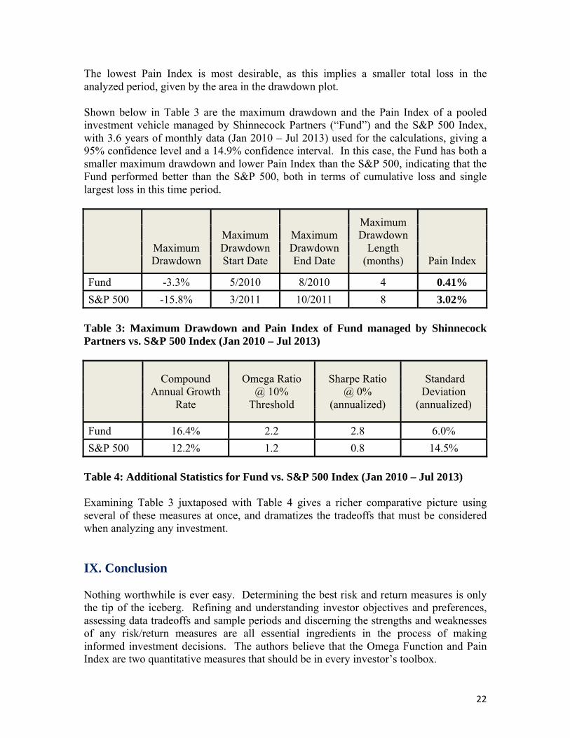
The lowest Pain Index is most desirable, as this implies a smaller total loss in the analyzed period, given by the area in the drawdown plot. Shown below in Table 3 are the maximum drawdown and the Pain Index of a pooled investment vehicle managed by Shinnecock Partners (“Fund”) and the S&P 500 Index, with 3.6 years of monthly data (Jan 2010 – Jul 2013) used for the calculations, giving a 95% confidence level and a 14.9% confidence interval. In this case, the Fund has both a smaller maximum drawdown and lower Pain Index than the S&P 500, indicating that the Fund performed better than the S&P 500, both in terms of cumulative loss and single largest loss in this time period.

Maximum Drawdown

Maximum Drawdown Start Date

Maximum Drawdown End Date

Maximum Drawdown

Length (months)

Pain Index

Fund -3.3% 5/2010 8/2010 4 0.41%

S&P 500 -15.8% 3/2011 10/2011 8 3.02%

Table 3: Maximum Drawdown and Pain Index of Fund managed by Shinnecock Partners vs. S&P 500 Index (Jan 2010 – Jul 2013)

Compound Annual Growth

Rate

Omega Ratio @ 10%

Threshold

Sharpe Ratio @ 0%

(annualized)

Standard Deviation

(annualized)

Fund 16.4% 2.2 2.8 6.0%

S&P 500 12.2% 1.2 0.8 14.5%

Table 4: Additional Statistics for Fund vs. S&P 500 Index (Jan 2010 – Jul 2013) Examining Table 3 juxtaposed with Table 4 gives a richer comparative picture using several of these measures at once, and dramatizes the tradeoffs that must be considered when analyzing any investment. IX. Conclusion Nothing worthwhile is ever easy. Determining the best risk and return measures is only the tip of the iceberg. Refining and understanding investor objectives and preferences, assessing data tradeoffs and sample periods and discerning the strengths and weaknesses of any risk/return measures are all essential ingredients in the process of making informed investment decisions. The authors believe that the Omega Function and Pain Index are two quantitative measures that should be in every investor’s toolbox.

23

References 1 Nassim Nicholas Taleb, Antifragile: Things That Gain from Disorder (Random House, 2012). 2 Joshua Ritchie, Investing: The History of the Stock Market, MintLife http://www.mint.com/blog/investing/the-history-of-the-stock-market (July 30, 2009). 3 Mike Dash, Tulipomania: The Story of the World’s Most Coveted Flower & the Extraordinary Passions it Aroused (Broadway Books, 2001 – first published, 1999). 4 Charles Mackay, Extraordinary Popular Delusions and the Madness of Crowds (Harriman House, 2003 – first published, 1841). 5 Andrew Beattie, Market Crashes: The Tulip and Bulb Craze, Investopedia, http://www.investopedia.com/features/crashes/crashes2.asp (July 7, 2013).

6 Aswath Damodaran, How Do We Measure Risk?, Stern School of Business at New York University, http://people.stern.nyu.edu/adamodar/pdfiles/valrisk/ch4.pdf (August 1, 2013). 7 A.W. Jones Advisors LLC, A.W. Jones: The First Hedge Fund, History of the Firm, http://www.awjones.com (July 30, 2013). 8 Michael Kaplan, “Meet A.W. Jones: The Anti-Nazi Spy and Journalist Who Started the First Hedge Fund in the World,” Business Insider, October 9, 2004 (http://www.businessinsider.com/aw-jones-started-the-first-hedge-fund-2012-10). 9 Jason Zweig, “A ‘Bucket List’ for Better Diversification,” The Wall Street Journal, February 8, 2013. 10 David Meko, Autocorrelation, The University of Arizona, http://www.ltrr.arizona.edu/~dmeko/notes_3.pdf (April 1, 2013). 11 Winton Capital Management et al., Assessing CTA Quality with the Omega Performance Measure, (September 2003). 12 Hayne E. Leland, “Beyond Mean-Variance: Performance Measurement in a Nonsymmetrical World,” Financial Analysts Journal (January/February 1999).

13 Peter G. Martin, Ulcer Index, An Alternative Approach to the Measurement of Investment Risk & Risk-Adjusted Performance, Freeman School of Business, Tulane University, http://www.freeman.tulane.edu/trading/pdf/UlcerIndexExplained.pdf (July 28, 2013).

24

14 University of Kentucky Archive, Skewness, http://www.uky.edu/Centers/HIV/cjt765/9.Skewness%20and%20Kurtosis.pdf (August 2, 2013). 15 Karl L. Wuensch, Skewness, Kurtosis, and the Normal Curve, East Carolina University, http://core.ecu.edu/psyc/wuenschk/docs30/Skew-Kurt.docx (July 30, 2013). 16 Con Keating, William F. Shadwick, Omega Functions and Omega Metrics: An Introduction to Omega, The Finance Development Centre of London, England, (2002). 17 Jack Schwager, “Trading Strategies: The Gain to Pain Ratio,” Active Trader, October 2012 (http://www.activetradermag.com/index.php/c/Trading_Strategies/d/The_Gain-to-Pain_ratio). 18 Alexei Chekhlov, Stanislav Uryasev and Michal Zabarankin, Drawdown Measure in Portfolio Optimization, International Journal of Theoretical and Applied Finance, 8(01), 13 – 58. 19 Marc Odo, The Pain Index and Pain Ratio, Zephyr Associates, Inc, http://www.styleadvisor.com/content/pain-index-and-pain-ratio (April 8, 2011). 20 Con Keating & William F. Shadwick, Omega Functions and Omega Metrics: An Introduction to Omega, The Finance Development Centre of London, England (2002). 21 Ana Cascon, Con Keating, William F. Shadwick, The Omega Function, The Finance Development Centre of London, England, (March 2003). 22 Keating et. al., (2002). 23 Keating et. al., (2002). 24 Vu Ngoc Nguyen, Omega Function: A Theoretical Introduction, Mathematics Department, University of Hawaii at Manoa, (2009). 25 Robert J. Frey, On the Ω Ratio, Applied Mathematics and Statistics Department, Stony Brook University, http://www.ams.sunysb.edu/~frey/Research/.../OmegaRatio/OmegaRatio.pdf (January 2009). 26 Odo, (2011).