NBER WORKING PAPER SERIES

RISK, MONETARY POLICY AND THE EXCHANGE RATE

Gianluca BenignoPierpaolo BenignoSalvatore Nisticò

Working Paper 17133http://www.nber.org/papers/w17133

NATIONAL BUREAU OF ECONOMIC RESEARCH1050 Massachusetts Avenue

Cambridge, MA 02138June 2011

We thank the editors, Daron Acemoglu and Michael Woodford. We also thank Marianna Bellòc, FabriceCollard, Charles Engel, Max Gillman, Hande Küçük-Tuger, Albert Marcet, Alessandro Rebucci, MartinUribe, seminar participants at Cardiff Business School and Trinity College Dublin and participantsat the NBER's Twenty-sixth Annual Conference on Macroeconomics for helpful comments, MatteoCiccarelli for sharing his RATS codes for PanelVAR estimation and analysis, and Federica Romeifor excellent research assistance. Financial support from and ERC Starting Independent Grant is gratefullyacknowledged. The views expressed herein are those of the authors and do not necessarily reflect theviews of the National Bureau of Economic Research.

NBER working papers are circulated for discussion and comment purposes. They have not been peer-reviewed or been subject to the review by the NBER Board of Directors that accompanies officialNBER publications.

© 2011 by Gianluca Benigno, Pierpaolo Benigno, and Salvatore Nisticò. All rights reserved. Shortsections of text, not to exceed two paragraphs, may be quoted without explicit permission providedthat full credit, including © notice, is given to the source.

Risk, Monetary Policy and the Exchange RateGianluca Benigno, Pierpaolo Benigno, and Salvatore NisticòNBER Working Paper No. 17133June 2011JEL No. E0,E43,E52,F3,F31,F41

ABSTRACT

In this research, we provide new empirical evidence on the importance of time-varying uncertaintyfor the exchange rate and the excess return in currency markets. Following an increase in monetarypolicy uncertainty, the dollar exchange rate appreciates in the medium run, while an increase in thevolatility of productivity leads to a dollar depreciation. We propose a general-equilibrium theory ofexchange rate determination based on the interaction between monetary policy and time-varying uncertaintyaimed at understanding these regularities. In the model, the behaviour of the exchange rate followingnominal and real volatility shocks is consistent with the empirical evidence. Furthermore we showthat risk factors and interest-rate smoothing are important in accounting for the negative coefficientin the UIP regression.

Gianluca BenignoLondon School of EconomicsDepartment of EconomicsHoughton StreetLondon WC2A 2AE ENGLANDg.benigno@lse.ac.uk

Pierpaolo BenignoDipartimento di Scienze Economiche e AziendaliLuiss Guido CarliViale Romania 3200197 RomeITALYand EIEFand also NBERpbenigno@luiss.it

Salvatore Nisticò Università di Roma "La Sapienza" Dipartimento di Scienze Economiche e Aziendali viale Romania 32 00197 Rome - Italy and LUISS Guido Carli salnisti@gmail.com

1 Introduction

One of the main features of the recent financial crisis has been the increase in financial and

macroeconomic volatility. Currency markets have not been an exception: foreign exchange

rate volatility has surged and large swings in the dollar exchange rate have occurred. How do

changes in volatility affect exchange rates? Is the source of volatility, nominal or real, relevant

for determining exchange rate fluctuations?

These are the questions that we address in this research by providing an empirical and

theoretical analysis on the link between uncertainty and the exchange rate. The focus on uncer-

tainty belongs to the tradition in international finance that has emphasized how variations in

risk over time are essential for understanding the exchange rate. In fact, the large biases in the

foreign-exchange forward premium that have been documented since Bilson (1981) and Fama

(1984) constitute a compelling evidence of variations in risk premia as a rational-expectations

explanation of the link between exchange rates and interest rates. Evidence of a time-varying

risk component of the excess return in foreign-exchange market is further documented by the

recent work of Menkhoff, Sarno, Schmeling and Schrimpf (2010), who show that deviations from

Uncovered Interest-rate Parity (UIP) can be accounted for in terms of compensation for risk.1

They identify global foreign exchange volatility as a key factor.

We propose a theory of exchange rate determination based on exogenous risk factors in which

the link between risk and the nominal exchange rate is guided by monetary policy through

interest-rate rules.2 The aim is to understand the role of exogenous risk factors in explaining

the main regularities that we observe in international finance. To this purpose, we depart from

most of the existing models of exchange rate determination, which study the impact of the first

moments of exogenous variables on the nominal exchange rate, and examine the exchange rate’s

response to changes in the volatility of nominal and real shocks.3 Moreover, the structure upon

which we build our analysis between risk factors and exchange rates is a theory of nominal

exchange rate determination based on interest rate rules (Benigno and Benigno, 2008).4

This research contributes to the literature from an empirical and a theoretical perspective.

In our empirical analysis we provide new evidence that justifies our focus on risk factors: the

novelty of our contribution is to examine the role of nominal and real stochastic volatilities

for the behavior of exchange rates in an otherwise standard open-economy VAR. We find that

volatility shocks do matter for the equilibrium level of interest and exchange rates and that the

exchange rate tends to appreciate in response to an increase in nominal volatility (both of the

discretionary shock to monetary policy and of the inflation target) and to depreciate following

1Engel (2010) provides further evidence on this even by looking at the real version of the UIP and shows thatthe expected appreciation of high-yield currencies is combined with a relatively stronger currency.

2In what follows we refer to risk, uncertainty and stochastic volatility in an interchangeable way.3Hodrick (1989) and Obstfeld and Rogoff (2001) in a flexible- and sticky-price environment, respectively, relate

the nominal exchange rate to monetary uncertainty through alternative specifications of money demand.4This implies that the parameters of the policy rules (as opposed to preferences to money demand) become

crucial in shaping exchange rate dynamics and in determining to what extent nominal or real disturbances matterfor the nominal (and real) exchange rate.

1

an increase in real volatility (of the productivity shock). Moreover, the stylized facts reported

by Eichenbaum and Evans (1995) about the response of interest and exchange rates to a shock

to the level of the monetary policy instrument are not affected by the explicit consideration of

time-varying volatility elements in the VAR.

In our theoretical model, the key channel through which exchange rates and uncertainty are

related is a simple hedging motive. An increase in uncertainty does not necessarily lead to a

depreciation of the currency: what matters is whether the currency is relatively safer when there

are bad news. In this respect, uncertainty may improve the hedging properties of the currency

leading to an increase in its demand and thereby an appreciation.

We develop a two-country open-economy model along the lines of Benigno and Benigno

(2008), extended in two dimensions. As in Benigno and Benigno (2008), we assume differentiated

home and foreign produced goods, international market completeness, nominal price rigidities

and interest rate rules; here, however, we allow for a more general specification of preferences

as in Epstein and Zin (1989) and for stochastic volatility in the exogenous processes driving the

economy.

In this direction, our contribution to the literature is to provide a general-equilibrium per-

spective on the ability of currently used models with stochastic volatility to explain international

macro-finance facts.5 From a modelling point of view, the general equilibrium analysis is crucial

for examining the transmission mechanism of risk factors and generating a non-trivial interac-

tion between shocks and the variables of interests. From an empirical point of view, the general

equilibrium analysis allows us to compare the model’s performance with the shocks and factors

highlighted in the VAR.

The assumption of time-varying exogenous uncertainty entails non-trivial issues in the so-

lution of the model. To this end, we apply a new method that we have recently developed for

general dynamic stochastic models with time-varying uncertainty (Benigno, Benigno and Nis-

tico, 2010). The main result of our previous work is that a second-order approximation of the

model is sufficient to account for a distinct and direct role of time-varying uncertainty on the

endogenous variables, provided that the structural shocks are conditionally linear. In contrast,

recent works have emphasized the need of relying on a third-order approximation (see Fernandez-

Villaverde and Rubio-Ramirez, 2010).6 Our method has several advantages: it simplifies the

computational burden, it reduces the degree of freedom that a third-order approximation would

generate when evaluating the model performance through a calibration exercise and, finally, it

allows to evaluate time-varying risk premia, which in our case are second-order terms, through

just a first-order approximation of the equilibrium conditions.

For a special case of our general model we are able to obtain analytical results. When

purchasing power parity holds, prices are flexible and monetary policy is specified as a Taylor

5As we will discuss below, most of the models that have been developed recently specify exogenous process forconsumption and/or output.

6The key difference is that our first-order approximation still displays heteroskedasticity and is the best ap-proximation in the class of conditionally-linear processes.

2

rule that reacts to either PPI or CPI inflation, we obtain that an increase in the domestic

volatilities of the nominal shocks appreciate the nominal exchange rate consistently with our

empirical findings. Theoretically the excess return on home currency bonds decreases with an

increase in nominal risk factors.

While this simple model is partly successful in capturing the link between nominal risk factors

and the exchange rate, it fails in replicating other key international finance regularities. In fact

the implied slope coefficient from a UIP regression would still be positive. We then consider the

case in which policy authorities smooth interest rates over time and find that, conditional on

shocks to the monetary policy instrument, it is possible to obtain a negative coefficient in the

UIP regression which becomes more negative as the smoothing coefficient increases.

From a theoretical point of view we then explore the role of Epstein-Zin preferences. First,

in an open economy, cross-country surprises in utility influence the international distribution of

wealth so that equilibrium quantities are also affected by the preference specification, unlike in

the closed-economy case. Second, if we focus on the case in which the subjective discount factor

is very close to the unitary value, then the surprises to utility depend, up to a first order, only

on the stochastic trend in world productivity. The implication is that, in this case, nominal

stochastic discount factors are highly correlated across countries, an aspect that is consistent

with a global explanation for risk premia.

We then evaluate quantitatively the properties of our model by calibrating it following the

recent empirical literature (see, e.g. Lubik and Schorfeide, 2005). We focus on a small set of facts

that are related to exchange rates. The response of exchange rates and excess returns to volatility

shocks is consistent with our empirical findings. Moreover, we show that the specification of

monetary policy and the presence of stochastic volatility terms is crucial for obtaining a negative

coefficient in the UIP regression (as discussed in Backus, Gavazzoni, Telmer and Zin, 2010).

Related Literature

This paper is related to different strands of literature. From an empirical point of view,

we build on the early analysis of Clarida and Gali (1994) and Eichenbaum and Evans (1995),

which have examined the effects of monetary shocks on the exchange rate. Our contribution is

to assess the role of real and nominal uncertainty on the exchange rate whereas their focus is on

the innovation in real and nominal shocks.

From a theoretical perspective there are two key elements in our analysis: stochastic volatil-

ity and monetary policy. The emphasis on exogenous risk factors is not novel in exchange rate

economics: early contributions by Frankel and Meese (1987) in a partial equilibrium setting,

and Hodrick (1989) in general equilibrium, have pointed out the role of uncertainty in explain-

ing exchange rate determination. More recently Obstfeld and Rogoff (2002) have studied the

role of risk factors in a general equilibrium model when nominal prices are sticky, focusing on

money supply as the monetary-policy instrument. Our paper follows this tradition in inter-

national finance and it is also connected to a more recent macroeconomic literature that has

3

examined the role and the effects that risk or uncertainty have on macroeconomic variables

(see for example Bloom, 2009, Bloom, Floetotto and Jaimovich, 2009 and Fernandez-Villaverde,

Guerron-Quintana, Rubio-Ramirez and Uribe, 2010).

The importance of monetary policy using interest-rate rules in exchange rate determina-

tion has been analyzed in Benigno and Benigno (2008) while its role for the understanding of

the uncovered interest rate parity puzzle has been first highlighted by McCallum (1994) and

more recently by Backus, Gavazzoni, Telmer and Zin (2010). The latter authors have recasted

McCallum’s insight in a microfounded setting endogenizing the currency risk premium that is

exogenous in McCallum’s model.

Our work is also related to a fast-growing literature in international macro-finance that has

developed models of the risk premium based on specifications of the stochastic discount factors

derived from alternative preferences. Bansal and Shaliastovich (2009) relies on Epstein-Zin pref-

erences combined with long-run risk, Backus et al. (2010) emphasizes the role of monetary policy

for addressing the uncovered interest rate parity puzzle in nominal terms, Gavazzoni (2009) re-

lies on Epstein-Zin preferences combined with stochastic volatility, Moore and Roche (2010) and

Verdelhan (2010) propose models based on external habit with preferences a la Campbell and

Cochrane (1999). While we share some of the features of these studies, our analysis follows a

general equilibrium approach by combining macro and financial market equilibrium and builds

upon a theory of nominal exchange rate determination based on interest rate rules. The latter

aspect is important insofar as we want to address, from a model perspective, the UIP puzzle in

nominal rather then in real terms as most of these models do.

2 Empirical evidence

In this section, we provide new empirical evidence on the importance of time-varying uncer-

tainty in open economies through a simple VAR analysis, along the lines of Eichenbaum and

Evans (1995), which we take as our empirical benchmark. We aim at providing a quantita-

tive assessment on the effects that innovations to the volatility of underlying disturbances may

have on the level of macro variables of interest. In particular we focus on the conditional

time-varying volatilities of three specific shocks, that are going to play a relevant role in the the-

oretical model of the next sections: the conditional volatility of the monetary-policy shock, of

the inflation-target shock and of the productivity shock.7 Our focus will be mainly to study how

these shocks affect the nominal (and real) exchange rate and the foreign currency risk premium

which captures the deviations from UIP. However, we will also look at the responses of output,

inflation and the yield curve. Moreover, we will evaluate whether the results of Eichenbaum

and Evans (1995), and investigated by a large body of subsequent literature, are robust to the

inclusion of time-varying volatility into the picture.

7In our model, the monetary policy shock represents a shock to the systematic component of the interest raterule. The inflation target is also part of the interest rate rule and represents the target with respect to which anydeviation of actual inflation triggers the policy response.

4

We use monthly data for the G7 countries on the sample period ranging from March 1971

through September 2010, and estimate a VAR with six lags for each pair of countries that

includes the US.8 We consider a benchmark specification with seven macroeconomic variables,

in the spirit of Eichenbaum and Evans (1995). To this set of macro “level” variables, we then

add three time series describing the time-varying volatilities of the monetary-policy shock (uξ,t),

the inflation-target shock (uπ,t) and the productivity shock (ua,t). The “level” variables that we

consider are the US nominal Federal Funds Rate (i) indicating the stance of monetary policy,

the US and foreign Industrial Production Indexes (y, y∗) measuring the domestic and foreign

real activity, the US CPI Index (p) capturing the domestic price level, the foreign short-term

nominal interest rate measured by the 3-month Treasury Bill rate (i∗), the slope of the US term

structure computed as the difference between the 10-year Treasury Constant Maturities rate

and the 3-month Treasury Bill rate (isl ≡ i10y − i3m) and the real exchange rate, defined as

q ≡ s + p∗ − p where s denotes the nominal exchange rate, expressed in terms of units of USD

needed to buy one unit of foreign currency.9 As such, an increase in q (or s) denotes a US Dollar

real (nominal) depreciation. All variables are in logs, except for the interest rates which are

monthly percentage points.

2.1 Measuring Time-varying Volatility

We now explain how we build the three conditional volatilities of interest. For the conditional

volatility of the monetary-policy shock we use daily data from the Federal Funds futures markets,

following Kuttner (2001), among others.

In particular, denoting with f0t,d the spot-month futures rate on day d for a contract with

delivery in month t (with day d belonging to month t) we can interpret f0t,d as the conditional

time−d expectation of the average funds rate in month t, plus a stochastic risk premium µ:

f0t,d = Ed

1

mt

∑j∈t

i1,j + µ0t,d,

wheremt is the number of days in month t and i1 is the daily interest rate. To extract information

about revisions in time−d expectations about future monetary policy actions from data on f ,

Kuttner (2001) suggests to use the daily change in the futures rate, scaled up to account for the

number of days in month t that are affected by the surprise: mtmt−d(f0

t,d − f0t,d−1). This measure

seems particularly appealing because it reduces the distortions associated with the time variation

in the risk premium µ.

As to our case, we use data on 1-month futures rates rather than spot-month rates, f1t,d,

8Many specifications of our empirical analysis, like the lag-order of the main VAR, the use of a price-level indexinstead of inflation, and the choice to display one-standard deviation bands in the impulse-response analysis, areborrowed from our empirical benchmark, Eichenbaum and Evans (1995), to which we seek to relate our results.

9We depart from Eichenbaum and Evans (1995), besides by including three volatility measures, by consideringthe slope of the US yield curve isl,t, on the one hand, while disregarding the measure of non-borrowed reserves,on the other hand.

5

where day d belongs to month t − 1 rather than t. As a consequence, any revision in policy

expectations reflected in a daily change of the futures rate is related to the full month t, rather

than a fraction of it. Therefore, in our case we can measure day−d revisions in expectations

about next-month monetary policy actions using the simple daily change in the futures rate:

(f1t,d − f1

t,d−1). In what follows we will denote with u2ξ,t the variance of the monetary policy

surprise in month t + 1 conditionally on information available in month t and we use, as an

approximate measure of such conditional variance, the empirical second moment, within month

t, of daily revisions in expectations of time-t+ 1 monetary policy actions:

uξ,t ≈

√√√√ 1

mt

mt∑d=2

(f1t,d − f1

t,d−1)2.

Since data for the Fed funds futures rates are only available starting October 1988, we

complete the time series with realized volatilities, within the month, computed using daily data

on the effective federal funds rate – net of settlement Wednesdays – standardized to the mean

and variance of the measure coming from the futures market, for the period where the two

measures overlap (correlation over that period is about .6)

For the inflation-target shock, we measure the conditional volatility with the Merrill Lynch

Option Volatility Estimate (MOVE). Movements in the inflation target can produce parallel

shifts in the yield curve.10 Indeed the MOVE Index can capture the volatility of this level factor

since it is a yield curve weighted index of the normalized implied volatility on 1-month Treasury

options, which are weighted on the 5, 10, and 30 year contracts. Since this index starts only

in 1989, we complete the time series with the realized volatility, within the month, computed

using daily data on US 10-year Treasury bonds; since the MOVE is an index, moreover, we

standardize it to the mean and variance of the realized volatility, for the period where the two

measures overlap (correlation over that period is about .8).

Finally, we build an approximate measure of the volatility of the productivity shock using the

stock market option-based implied volatility, the VIX index (monthly averages of daily data).

However, since data for the VIX are only available starting January 1990, we follow the approach

of Bloom (2009) and complete the time series with within-month realized volatilities computed

using daily returns on the S&P500, standardized to the mean and variance of the VIX, for the

period where the two measures overlap (correlation over that period is about .9).

As a last step, since all above measures are based on implied and realized volatilities, we

construct the conditional volatilities considering the fitted values of an AR(1) regression for each

indicator, similarly to Bekaert and Engstrom (2009). Figure 1 displays the dynamic properties

of the obtained indicators.

10This is true in the theoretical model presented later in the paper but we leave the details for future work.

6

1970 1980 1990 2000 20100

5

10

15

20Conditional Volatility of the Monetary Policy Shock (Fed Funds Futures)

1970 1980 1990 2000 20100

10

20

30Conditional Volatility of the Inflation Target Shock (MOVE Index)

1970 1980 1990 2000 20100

20

40

60Conditional Volatility of the Productivity Shock (VIX Index)

Figure 1: Time-varying conditional volatilities, standard deviations in percentage points. Note: the y-axis of thebottom panel has been truncated at 60 for the sake of readability; the value of the index around Black Mondayis actually about 87.

2.2 VAR Analysis

For each pair of the G7 countries that includes the US, we then estimate the following VAR(p)

model

yt = A(L)yt−1 + et, (1)

where the data vector is defined as yt ≡ [uξ,t, ua,t, uπ,t, yt, pt, it, isl,t, i∗t , qt, y

∗t , ]′, and the lag-

order is six. This ordering allows for a contemporaneous response of the interest rate to domestic

output and the price level, consistently with a Taylor-type monetary policy rule and with our

empirical benchmark (see Eichenbaum and Evans, 1995). As to the order in which the volatility

measures enter the VAR, our choice is driven by how volatility is modelled in the theoretical

framework of the next sections. Indeed, we build a model in which volatility shocks are allowed

to have contemporaneous effects on the endogenous variables; however, in order to apply the

approximation methods developed by Benigno, Benigno and Nistico (2010), we restrict our

attention to conditionally-linear stochastic processes for the underlying structural disturbances

of our theoretical model, implying contemporaneous orthogonality between “level” shocks and

volatility measures. In order to be consistent with these features of our theoretical approach,

therefore, in the VAR we place the volatility measures before all the other variables. As to the

volatility measures, since the MOVE index might also be affected by the volatility of monetary

policy or productivity shocks, we place it last among the three volatility indexes. On the other

hand, since the monetary-policy volatility measure is built directly from data on the Federal

7

0 25 500

0.5

1US FFR

0 25 500.5

0

0.5

1US FFR

0 25 500.5

0

0.5

1US FFR

0 25 500.5

0

0.5

1US FFR

0 25 500.5

0

0.5

1US FFR

0 25 500.5

0

0.5

1US FFR

0 25 501

0.5

0

0.5CAN RER

0 25 501.5

1

0.5

0FRA RER

0 25 502

1

0GER RER

0 25 502

1

0

1ITA RER

0 25 502

1

0

1JAP RER

0 25 501

0.5

0

0.5UK RER

0 25 500.5

0

0.5CAN EXR

0 25 501

0.5

0

0.5FRA EXR

0 25 501

0.5

0

0.5GER EXR

0 25 501

0.5

0

0.5ITA EXR

0 25 501

0.5

0

0.5JAP EXR

0 25 501

0.5

0

0.5UK EXR

0 25 500.5

0

0.5SLOPE

0 25 500.5

0

0.5SLOPE

0 25 500.5

0

0.5SLOPE

0 25 500.5

0

0.5SLOPE

0 25 500.5

0

0.5SLOPE

0 25 500.5

0

0.5SLOPE

Figure 2: Dynamic responses to an orthogonalized innovation to the Federal Funds Rate. Each column reports,for each country pair, the responses of the US Federal Funds rate (i), the Real Exchange Rate (q), the foreigncurrency risk premium (exr), the slope of the US term structure (isl). x-axes: months, y-axes: annual percentagepoints. Country pairs are, respectively, US-Canada, US-France, US-Germany, US-Italy, US-Japan, US-UK.

Funds Market, we see it as very tightly related to monetary policy: we therefore assume that it

is not affected contemporaneously by any other volatility measure and thus place it first.

Figures 2 through 5 display the dynamic response of selected variables to, respectively, a

“classic” monetary-policy shock (the orthogonalized innovation to the level of the Federal funds

rate), an innovation to the volatility of the monetary-policy shock, an innovation to the volatility

of the shock to the inflation target and an innovation to the volatility of the productivity shock.

Each panel reports the point estimate of the impulse response function – the solid line – and the

associated one-standard-deviation confidence intervals – the dashed lines. In each figure, the first

row displays the dynamic response of the US Federal Funds Rate, the second row the response

of the real exchange rate, the third the response of the excess return on foreign currency, and

the last one shows the response of the slope of the yield curve.11 In particular, the excess return

on foreign currency is defined as

exrt ≡ i∗1,t − i1,t + Et∆st+1,

and measures deviations from the UIP condition.

Figure 2 addresses the robustness of the findings of Eichenbaum and Evans (1995). The

responses to a contractionary shock to monetary policy seem virtually unaffected by the explicit

11We do not report the responses of the nominal exchange rate, since they are very similar to those of the realexchange rate.

8

0 25 500.5

0

0.5US FFR

0 25 500.5

0

0.5US FFR

0 25 500.5

0

0.5US FFR

0 25 500.5

0

0.5US FFR

0 25 500.5

0

0.5US FFR

0 25 500.5

0

0.5US FFR

0 25 500.5

0

0.5

1CAN RER

0 25 501

0

1FRA RER

0 25 502

1

0

1GER RER

0 25 501

0.5

0

0.5ITA RER

0 25 501

0

1

2JAP RER

0 25 502

1

0

1UK RER

0 25 500.2

0

0.2CAN EXR

0 25 500.5

0

0.5FRA EXR

0 25 500.5

0

0.5GER EXR

0 25 500.5

0

0.5ITA EXR

0 25 500.5

0

0.5JAP EXR

0 25 500.2

0

0.2UK EXR

0 25 500.2

0

0.2SLOPE

0 25 500.2

0

0.2SLOPE

0 25 500.2

0

0.2SLOPE

0 25 500.2

0

0.2SLOPE

0 25 500.2

0

0.2SLOPE

0 25 500.2

0

0.2SLOPE

Figure 3: Dynamic responses to an orthogonalized innovation to the volatility of the monetary-policy shock.Each column reports, for each country pair, the responses of the US Federal Funds Rate (i), the Real ExchangeRate (q), the foreign currency risk premium (exr), the slope of the US term structure (isl). x-axes: months, y-axes: annual percentage points. Country pairs are, respectively, US-Canada, US-France, US-Germany, US-Italy,US-Japan, US-UK.

consideration of the interplay between time-varying volatility and the “level” variables. In par-

ticular, a positive innovation to the Federal Funds Rate implies a significant appreciation of the

USD, on impact. Moreover, the exchange rate keeps appreciating also in the transition, and

does not start depreciating but in the medium run. Second, the spread between foreign and do-

mestic short-term interest rates decreases gradually through the implied, less-than-proportional,

increase in the foreign one (not shown). Finally, the two results above drive the persistent devi-

ations from UIP shown in the third row, in the form of positive excess returns on US securities.

Additionally, Figure 2 also shows the negative response of the slope of the yield curve.

Figures 3, 4 and 5 present our new evidence on the importance of volatility shocks. The

first result, common to all three figures, is that shocks to volatility indeed do affect the level of

the other macro variables, although with different magnitudes and significance across variables

and shocks. Hence volatility does have a distinct and direct effect which will be important in

characterizing our theoretical model.

In particular, Figure 3 shows the responses to an orthogonalized innovation to the volatility

of the monetary-policy shock. The response of the exchange rate (second row) is ambiguous.

The point estimate indicates that an increase in the volatility of the monetary-policy shock

strengthens the US dollar. However, this is not particularly significant (except for the case

of the UK and, marginally, Germany). Later, we are going to evaluate if results change by

exploiting the panel dimension of our dataset. The third row shows that an increase in the

9

0 25 500.2

0

0.2US FFR

0 25 500.2

0

0.2US FFR

0 25 500.2

0

0.2US FFR

0 25 500.2

0

0.2US FFR

0 25 500.5

0

0.5US FFR

0 25 500.5

0

0.5US FFR

0 25 500.5

0

0.5CAN RER

0 25 502

1

0

1FRA RER

0 25 501

0.5

0

0.5GER RER

0 25 502

1

0

1ITA RER

0 25 501

0

1

2JAP RER

0 25 501

0

1UK RER

0 25 500.5

0

0.5CAN EXR

0 25 500.2

0

0.2FRA EXR

0 25 500.2

0

0.2GER EXR

0 25 500.5

0

0.5ITA EXR

0 25 500.5

0

0.5JAP EXR

0 25 500.5

0

0.5UK EXR

0 25 500.1

0

0.1SLOPE

0 25 500.1

0

0.1SLOPE

0 25 500.1

0

0.1SLOPE

0 25 500.1

0

0.1SLOPE

0 25 500.1

0

0.1SLOPE

0 25 500.1

0

0.1SLOPE

Figure 4: Dynamic responses to an orthogonalized innovation to the volatility of the inflation-target shock.Each column reports, for each country pair, the responses of the US Federal Funds Rate (i), the Real ExchangeRate (q), the foreign currency risk premium (exr), the slope of the US term structure (isl). x-axes: months, y-axes: annual percentage points. Country pairs are, respectively, US-Canada, US-France, US-Germany, US-Italy,US-Japan, US-UK.

volatility of the monetary-policy shock induces significant and persistent deviations from UIP,

in the form of positive excess returns on foreign securities. This result is mainly driven by the

response of the spread in the short-term interest rate: the domestic rate falls significantly, and

proportionately more than the foreign one, implying an increase in the spread by a magnitude

of 5-10 basis points (not shown). The estimated response of the slope of the US yield curve, is

positive on impact and keeps rising for a few months before reverting back to mean; it remains,

however, significantly above the steady-state level for quite some time, regardless of the pair

considered (except for the case of Germany, for which the effect dies out within six months).

Figure 4 shows the response to an orthogonalized innovation to the volatility of the inflation-

target shock. Here, the implications for the exchange rate are very interesting. Indeed, while

the response is weak on impact and not always significant, the point estimates indicate that

an increase in the volatility of the inflation-target shock tends to appreciate the exchange rate

(with the notable exception of Japan) in the medium run. This is a particularly appealing

result considering the specific nature of the shock, which is indeed related to the medium-run

target level for the inflation rate. This pattern is also reflected in the dynamic response of

the foreign-currency risk premium: while the short-term response is ambiguous, the estimated

impulse-response functions indicate that in the medium run a higher volatility of the inflation-

target shock produces a lower foreign currency risk premium, consistently with the appreciation

of the domestic currency. Finally, the estimated responses of the nominal interest rate and the

10

0 25 500.5

0

0.5US FFR

0 25 500.5

0

0.5US FFR

0 25 500.5

0

0.5US FFR

0 25 500.5

0

0.5US FFR

0 25 500.5

0

0.5US FFR

0 25 500.5

0

0.5US FFR

0 25 500.5

0

0.5

1CAN RER

0 25 501

0

1FRA RER

0 25 501

0

1

2GER RER

0 25 501

0

1

2ITA RER

0 25 500

0.5

1

1.5JAP RER

0 25 501

0

1UK RER

0 25 500.2

0

0.2CAN EXR

0 25 500.2

0

0.2FRA EXR

0 25 500.2

0

0.2GER EXR

0 25 500.2

0

0.2ITA EXR

0 25 500.5

0

0.5JAP EXR

0 25 500.2

0

0.2UK EXR

0 25 500.2

0

0.2SLOPE

0 25 500.2

0

0.2SLOPE

0 25 500.2

0

0.2SLOPE

0 25 500.2

0

0.2SLOPE

0 25 500.2

0

0.2SLOPE

0 25 500.2

0

0.2SLOPE

Figure 5: Dynamic responses to an orthogonalized innovation to the volatility of productivity shocks. Eachcolumn reports, for each country pair, the responses of the US Federal Funds Rate (i), the Real Exchange Rate(q), the foreign currency risk premium (exr), the slope of the US term structure (isl). x-axes: months, y-axes:annual percentage points. Country pairs are, respectively, US-Canada, US-France, US-Germany, US-Italy, US-Japan, US-UK.

slope of the yield curve are not very precise. However, the point estimates suggest a positive

response of both the domestic short-term interest rate and the term spread. Again, we will look

further into this evidence by exploring the panel dimension of the data.

Figure 5 studies the responses to the conditional volatility of the productivity shock. In

particular, the response of the exchange rate is quite clear: although with different timing and

magnitude across country pairs, an increase in the volatility of the productivity shock tends

to depreciate the exchange rate, mostly on impact. No significant deviation from UIP arises

with the notable exception of Japan. Finally, the estimated response of the slope of the yield

curve is muted on impact, but it becomes substantially and significantly positive after about six

months and stays significantly positive until about two years after the shock, peaking at about

10-15 basis points after about one year. This response is virtually identical across all considered

country pairs.

2.3 Exploring the Panel Dimension of the Dataset

The empirical evidence of the last section points toward an interesting and non-trivial role of

stochastic volatility for macro-financial variables, both domestic (like the short-term interest

rate or the term spread) and international (like the exchange rate and deviations from the

UIP). Although the point estimates in the pair-wise analysis suggest clear trends in the impulse

responses of key variables, such trends are sometimes polluted by sampling uncertainty. In order

11

0 10 20 30 40 50

0.2

0.1

0

0.1US FFR

0 10 20 30 40 501

0.5

0

RER

0 10 20 30 40 500.1

0

0.1

0.2

EXR

0 10 20 30 40 50

0

0.1

0.2SLOPE

Two country

0 10 20 30 40 50

0.2

0.1

0

0.1US FFR

0 10 20 30 40 501

0.5

0

RER

0 10 20 30 40 500.1

0

0.1

0.2

EXR

0 10 20 30 40 50

0

0.1

0.2SLOPE

Mean Group

0 10 20 30 40 50

0.2

0.1

0

0.1US FFR

0 10 20 30 40 501

0.5

0

RER

0 10 20 30 40 500.1

0

0.1

0.2

EXR

0 10 20 30 40 50

0

0.1

0.2SLOPE

Pooled

Figure 6: Dynamic responses to an orthogonalized innovation to the volatility of the monetary-policy shock.Each column reports, for each empirical approach, the responses of the US Federal Funds Rate (i), the RealExchange Rate (q), the foreign currency risk premium (exr), the slope of the US term structure (isl). x-axes:months, y-axes: annual percentage points. “Two-country”: single VAR, US-vs-G6 countries (Japan excluded);“Mean-Group”: average statistics from pair-specific VARs (from section 2.2); “Pooled”: single Pooled Panel VARestimation.

to isolate more effectively the common components across countries, here we exploit the panel

dimension of our dataset using three methods.12

The first approach is to define a Two-Country version of our empirical model. We take

the home country as describing the US economy, while the foreign country is a GDP-weighted

average of the other G7 countries, Japan excluded.13 The relevant exchange rate is therefore

a multilateral exchange rate, while the foreign currency risk premium is actually the expected

excess return on a portfolio of several foreign currencies, with the portfolio share of each currency

being proportional to the respective country size. The dynamic responses of the four variables

of interest are displayed in the first column of Figures 6 through 8, labeled “Two-Country”.14

The second approach is a Panel VAR Mean-Group estimation, in the spirit of Pesaran and

Smith (1995): we estimate a separate VAR model for each country-pair and then evaluate the

12For a thorough discussion of these and other empirical approaches for the analysis of dynamic macro panels,see Canova (2007, Ch. 8).

13As shown in the previous section, Japan is often an outlier with respect to the dynamic responses of theexchange rate and the foreign currency risk premium. These differences suggest that the Japanese currencybehaves in a somewhat peculiar way vis-a-vis the USD, for which the enormous and persistent positions in theyen carry-trade strategy might possibly play a key role. For this reason, we disregard Japan for the remaining ofthe section.

14This corresponds to the Aggregate Time Series estimator, as defined by Canova (2007), which we slightlymodify by aggregating the time series using a GDP-weighted average (rather than a simple average) as in Benignoand Nistico (2011), among others.

12

0 10 20 30 40 500.1

0

0.1

0.2US FFR

0 10 20 30 40 501

0.5

0

0.5RER

0 10 20 30 40 50

0.2

0.1

0

EXR

0 10 20 30 40 500.1

0

0.1SLOPE

Two country

0 10 20 30 40 500.1

0

0.1

0.2US FFR

0 10 20 30 40 501

0.5

0

0.5RER

0 10 20 30 40 50

0.2

0.1

0

EXR

0 10 20 30 40 500.1

0

0.1SLOPE

Mean Group

0 10 20 30 40 500.1

0

0.1

0.2US FFR

0 10 20 30 40 501

0.5

0

0.5RER

0 10 20 30 40 50

0.2

0.1

0

EXR

0 10 20 30 40 500.1

0

0.1SLOPE

Pooled

Figure 7: Dynamic responses to an orthogonalized innovation to the volatility of the inflation-target shock.Each column reports, for each empirical approach, the responses of the US Federal Funds Rate (i), the RealExchange Rate (q), the foreign currency risk premium (exr), the slope of the US term structure (isl). x-axes:months, y-axes: annual percentage points. “Two-country”: single VAR, US-vs-G6 countries (Japan excluded);“Mean-Group”: average statistics from pair-specific VARs (from section 2.2); “Pooled”: single Pooled Panel VARestimation.

mean of the estimated statistics of interest (namely the impulse-response function) across groups.

Our dataset is sufficiently long, along the time-series dimension, to support consistency of the

Mean-Group estimator. The impulse-responses of interest are displayed in the second column

of Figures 6–8. In this case, the exchange-rate response measures the average response that the

dollar bilateral exchange rate displays after a (domestic) level or volatility shock. Similarly, the

third panel of the column shows the average response of the foreign currency risk premium with

respect to the US dollar.

The third and final approach that we consider is the traditional Panel VAR Pooled estima-

tion: we pool cross section and (demeaned) time series, and estimate and analyze a VAR(p)

using the pooled series. This estimator, by construction, imposes the same dynamic structure

to all countries, vis-a-vis the US. Accordingly, also in this case the impulse-response functions

show an “average” response, capturing the common component across countries, of the bilateral

USD exchange rate and foreign risk premium.

Figures 6 through 8 display the dynamic response of selected variables to the three volatility

shocks that we analyze, for each method used. The variables are the US Federal Funds Rate

(i), the US Dollar Real Exchange Rate (q), the expected excess return on foreign currency with

respect to the US Dollar (exr) and the slope of the US yield curve (isl). In particular, the

“Pooled” approach, displayed in the third column of each figure, seems quite useful in order to

13

0 10 20 30 40 50

0.2

0.1

0

0.1US FFR

0 10 20 30 40 500.5

0

0.5

1RER

0 10 20 30 40 500.1

0

0.1

EXR

0 10 20 30 40 500.1

0

0.1

0.2SLOPE

Two country

0 10 20 30 40 50

0.2

0.1

0

0.1US FFR

0 10 20 30 40 500.5

0

0.5

1RER

0 10 20 30 40 500.1

0

0.1

EXR

0 10 20 30 40 500.1

0

0.1

0.2SLOPE

Mean Group

0 10 20 30 40 50

0.2

0.1

0

0.1US FFR

0 10 20 30 40 500.5

0

0.5

1RER

0 10 20 30 40 500.1

0

0.1

EXR

0 10 20 30 40 500.1

0

0.1

0.2SLOPE

Pooled

Figure 8: Dynamic responses to an orthogonalized innovation to the volatility of productivity shocks. Eachcolumn reports, for each empirical approach, the responses of the US Federal Funds Rate (i), the Real ExchangeRate (q), the foreign currency risk premium (exr), the slope of the US term structure (isl). x-axes: months, y-axes:annual percentage points. “Two-country”: single VAR, US-vs-G6 countries (Japan excluded); “Mean-Group”:average statistics from pair-specific VARs (from section 2.2); “Pooled”: single Pooled Panel VAR estimation.

derive more precise impulse responses.

By looking at Figures 6 through 8, the overall picture shows that the main results, made

in the previous section, are in fact reinforced considering the panel dimension of our data. In

particular, in response to an unexpected increase in the volatility of the monetary-policy shock,

Figure 6 shows that the US Dollar tends to appreciate while the foreign-currency risk premium

increases. The latter result is driven by the domestic short-term interest rate falling more

than the foreign one (not shown), which more than offsets the negative effect coming from the

appreciation of the exchange rate. The yield curve, moreover, becomes significantly steeper.

Following an increase in the volatility of the inflation-target shock, the real exchange rate

tends to appreciate in the medium term while the currency premium decreases, mainly as a

result of the significant increase in the Federal Funds Rate. The slope of the yield curve, as also

implied by the pair-wise analysis, does not seem to display any systematic response.

Finally, and again consistently with the evidence suggested by the pair-wise analysis of the

previous section, an increase in the volatility of the productivity shock depreciates the US dollar

and makes the yield curve significantly steeper. No clear effect is displayed by the foreign

currency risk premium, regardless of the significant decrease in the domestic interest rate.

The important conclusion that we can draw from this analysis is that indeed volatility does

matter. And it does matter also for traditional macro variables like real activity and the price

level, as Figure 9 shows. In response to an increase in volatility of the monetary-policy shock

14

0 25 505

4

3

2

1

0

1x 10 3

y

0 25 504

3

2

1

0x 10 3

p

u

0 25 505

4

3

2

1

0

1x 10 3

0 25 504

3

2

1

0

1x 10 3

ua

0 25 501

0

1

2

3

4x 10 3

0 25 501.5

1

0.5

0

0.5

1

1.5x 10 3

u

Figure 9: Dynamic responses of the domestic industrial production index (first row) and the domestic CPI(second row) to, respectively, a shock to the volatility of the monetary-policy instrument (uξ) (first column), ofthe productivity shock (ua) (second column) and of the inflation-target shock (uπ) (third column).

or to productivity, real activity substantially contracts and the price level falls, while a rise in

volatility of the inflation-target shock tends to bring CPI inflation to a permanently higher level

in the long-run and implies a temporary increase in real output. Finally, not displayed, the

impulse responses to an increase in the level of the monetary-policy shock are standard as in

the literature, with output falling and the prices rising in the short-run, consistently with the

standard “price puzzle”.15

3 International finance regularities

In the previous section, we have provided evidence that volatility shocks have important effects

on open-economy macro variables. In the next section, we are going to build a model in which

indeed time-varying uncertainty plays a role. To nail down the desiderata that our model should

meet, here we summarize the implications of our findings and report other empirical regularities

along which we would like our model to perform well. The sense in which we refer to these

facts (or puzzles) as international finance regularities relates to our focus on the joint behavior

of interest rates and exchange rates.

The empirical evidence on the importance of volatility shocks can be summarized along two

facts related respectively to the effects that volatility shocks have on the nominal (and real)

exchange rate and the deviations from UIP.

Fact 1 : An increase in the volatilities of the US monetary-policy and inflation-target shocks

appreciates the dollar exchange rate, especially in the medium run. On the other hand, an

increase in the volatility of the productivity shock depreciates the dollar exchange rate.

15See Figure 18 for the complete set of impulse-response functions for the Pooled Panel VAR.

15

Fact 2 : An increase in the volatilities of both the monetary-policy and the inflation-target

shocks generates significant and persistent deviations from UIP; in particular an increase in the

excess return of foreign-versus-domestic short-term bonds in the case of the monetary-policy

volatility shock and a decrease in the case of the inflation-target volatility shock.

The next fact is in common between our empirical analysis and the evidence reported by

Eichenbaum and Evans (1995).

Fact 3 : A positive innovation to the level of the monetary-policy shock (contractionary

policy shock) produces a persistent appreciation in both the real and nominal exchange rates

and a persistent deviations from the UIP in the form of positive excess returns on US securities.

To this list, we add another well-know fact, or puzzle, that we would like to address. While

our previous facts are conditional statements about how excess returns and exchange rate co-

move following different innovations (level or volatility shocks), another relevant empirical regu-

larity is related to the joint behavior of exchange and interest rates as captured by the negative

regression coefficient that arises from the UIP regression.

Fact 4 : The regression coefficient between exchange rate changes and the nominal interest

rate differential (UIP regression) is negative.

Related to the UIP puzzle, there is another one, recently discussed by Engel (2010), who

documents that high real interest rate countries tend to have currencies that are strong in real

terms and stronger than what can be explained by the real UIP. In particular, the puzzle comes

from the fact that while current international-finance models struggle to account for the negative

covariance between interest-rate differentials and exchange rate changes, those that succeed

invariably miss the negative covariance between the interest-rate differential and the level of

the exchange rate. Moreover, while the real interest-rate differential is negatively correlated

with the real one-step-ahead excess return on foreign-versus-domestic currency, such correlation

turns positive if we instead consider the “prospective excess return”, i.e. the expected cumulative

excess return over the infinite future.

Finally, we would like our model to be also consistent with the responses of output and prices

to the volatility shocks documented in Figure 9.

4 A two-country open economy model

To study the relationships between time-varying volatility and the exchange rate, we present a

two-country open-economy model along the lines of Benigno and Benigno (2008). In particular

we consider two extensions, whose relevance will be discussed later, which are important for the

model to be able to match the empirical facts discussed above: i) we allow for more general

recursive preferences as in the work of Epstein and Zin (1989, 1991) and Weil (1990) and ii)

we consider stochastic volatility for the exogenous processes driving the economy. The latter

addition, in particular, implies a careful treatment of the solution. To this end, we expound

the method developed by Benigno, Benigno and Nistico (2010) to show how we can handle in

16

a relatively easy way approximations of dynamic general equilibrium models with time-varying

uncertainty and at the same time characterize the effect of uncertainty on the variables of

interest.

4.1 Households

The world economy consists of two countries, Home and Foreign, and is populated by a con-

tinuum of agents of measure one: Home households lie on the interval [0, n], while Foreign

households on (n, 1] where n ∈ (0, 1). The population size is set equal to the range of goods

produced so that Home firms produce goods on [0, n], Foreign firms produce on (n, 1]. Home

households are indexed by j, Foreign households by i. Cjt denotes the level of consumption for

household j in period t and Ljt denotes its supply of working hours.

Preferences are recursive as in the framework of Epstein and Zin(1989, 1991) and Weil (1990).

In particular, we assume that for a generic household of type j recursive utility can be written

as

V jt =

(U(Cjt , Lt

)1−ρ+ β

(Et(V

jt+1)1−γ

) 1−ρ1−γ) 1

1−ρ

(2)

where ρ is a measure of the inverse of the intertemporal elasticity of substitution over the utility

flow, U(·), γ represents the risk aversion towards static wealth gambles, and β ∈ (0, 1) is the

household’s subjective discount factor. The classical expected utility model is nested under the

assumption ρ = γ.

The utility flow is a Cobb-Douglas index of aggregate consumption, C, and leisure, 1− L

U(Cjt , L

jt

)=(Cjt

)ψ(1− Ljt )1−ψ (3)

where ψ ∈ (0, 1) reflects the preference for consumption versus leisure. As it is well known, this

specification of preferences allows to disentangle the elasticity of substitution, 1/ρ, from the

risk-aversion coefficient.16

The aggregate consumption index C is a composite consumption good

C =

[v

1θC

θ−1θ

H + (1− v)1θC

θ−1θ

F

] θθ−1

, θ > 0 (4)

where CH and CF are the two consumption sub-indexes that refer, respectively, to the con-

sumption of Home-produced and Foreign-produced goods; θ, with θ > 0, is the elasticity of

intratemporal substitution and v ∈ (0, 1) represents the weight given to home-produced goods

in the aggregator C. Home bias in consumption arises when the weight given to Home goods is

higher than the size of the country, i.e. when v > n.

16See Swanson (2010) for how to compute risk-aversion toward consumption with Epstein-Zin preferences.

17

In the Foreign country, preferences have the same structure as in (2)

V ∗it =

(U(C∗it , L

∗it

)1−ρ+ β

(Et(V

∗it+1)1−γ) 1−ρ

1−γ

) 11−ρ

(5)

where the aggregate consumption bundle is given by

C∗ =

[v∗

1θC∗ θ−1

θH + (1− v∗)

1θC∗ θ−1

θF

] θθ−1

, (6)

for a different weight v∗ ∈ (0, 1) .

We introduce home bias in consumption following Benigno and De Paoli (2010). Specifically,

denoting with λ ∈ (0, 1) the (common) degree of openness of the two countries, the weights in

the consumption bundle are related to the country sizes through:

1− v = (1− n)λ,

v∗ = nλ.

The consumption bundles CH , CF , C∗H , C

∗F , are in turn Dixit-Stiglitz aggregators of the goods

produced in the two countries and are given by

CH =

[(1

n

) 1σ∫ n

0c (h)

σ−1σ dh

] σσ−1

CF =

[(1

1− n

) 1σ∫ 1

nc (f)

σ−1σ df

] σσ−1

, (7)

C∗H =

[(1

n

) 1σ∫ n

0c∗ (h)

σ−1σ dh

] σσ−1

C∗F =

[(1

1− n

) 1σ∫ 1

nc∗ (f)

σ−1σ df

] σσ−1

, (8)

where σ, with σ > 1, is the elasticity of substitution across the consumption goods produced

within a country. The appropriate consumption-based price indexes associated with C and C∗

are given respectively by

P =[vP 1−θ

H + (1− v) (PF )1−θ] 1

1−θ, (9)

P ∗ =[v∗P ∗1−θH + (1− v∗) (P ∗F )1−θ

] 11−θ

, (10)

where PH (P ∗H) is the price sub-index for Home-produced goods expressed in the Home (Foreign)

currency and PF (P ∗H) is the price sub-index for Foreign-produced goods expressed in the Home

(Foreign) currency. Moreover

PH =

[(1

n

)∫ n

0p (h)1−σ dh

] 11−σ

PF =

[(1

1− n

)∫ 1

np (f)1−σ dz

] 11−σ

, (11)

18

P ∗H =

[(1

n

)∫ n

0p∗ (h)1−σ dz

] 11−σ

P ∗F =

[(1

1− n

)∫ 1

np∗ (f)1−σ dz

] 11−σ

, (12)

where p (h) and p∗ (h) are the prices of the generic good h produced by the Home country in the

currencies of the Home and Foreign country respectively; while p (f) and p∗ (f) are the prices of

the generic good f produced by the Foreign country in the currencies of the Home and Foreign

country respectively. The law of one price holds across all individual goods: p(h) = Sp∗(h) and

p(f) = Sp∗(f), where S is the nominal exchange rate (the price of foreign currency in terms of

domestic currency). Therefore, equations (11) and (12), imply that PH = SP ∗H and PF = SP ∗F .

However, equations (9) and (10) show that, since Home and Foreign agents’ preferences are not

necessarily identical, there can be deviations from purchasing power parity unless v = v∗, that

is, P 6= SP ∗. Appropriately we measure the deviations from PPP through the real exchange rate

given by Q ≡ SP ∗/P. We also define the terms of trade in the Home country as T ≡ PF /PH.

Notice the following useful relationships between relative prices, the real exchange rate and

terms of trade

1 =

[v

(PHP

)1−θ+ (1− v)

(PFP

)1−θ], (13)

Q =

[v∗ + (1− v∗) (T )1−θ

] 11−θ

[v + (1− v) (T )1−θ

] 11−θ

, (14)

T =PFP

P

PH. (15)

Given the above-specified preferences, we can derive total demands of the generic good h, pro-

duced in country H, and of the good f, produced in country F:

yd(h) =

(p(h)

PH

)−σYH yd(f) =

(p(f)

PF

)−σYF (16)

where output aggregators YH and YF are appropriately defined

YH =

(PHP

)−θ (vC +

v∗(1− n)

nQθC∗

), (17)

YF =

(PFP

)−θ ((1− v)n

1− nC + (1− v∗)QθC∗

). (18)

We assume that asset markets are complete both at the domestic and international levels. In

particular households can trade in a set of state-contingent nominal securities denominated

in the Home currency which span all the uncertainty from one period to another.17 Each

17See Chari et al. (1998).

19

of these securities pays respectively only in one of the possible states of nature in the next

period. Let Bjt+1 the state-contingent payoff at time t + 1 of the portfolio of state-contingent

nominal securities held by household in the Home country at the end of period t. The value of

this portfolio can be written as Et[Mt,t+1Bjt+1] where Mt,t+1 represents the nominal stochastic

discount factor for discounting units of Home-currency wealth from a state of nature at time

t + 1 back to time t. This stochastic discount factor is unique, because of the complete-market

assumption, and equivalent to the price of a state-contingent security standardized by the time-t

conditional probability of occurrence of the state of nature at time t + 1 in which the security

pays. We can write the flow budget constraint that the Home households face as

Et[Mt,t+1Bjt+1] ≤ Bj

t +WtLjt +Dj

t − PtCjt ,

for each j, where Wt is the nominal wage in the Home country, determined in a common labor

market; Djt are nominal profits. Each household holds equal shares of all firms (domestic firms

are located on the interval [0, n] and the size of the Home population is normalized to n); there

is no trade in firms’ shares. Households are subject to a standard limit on their borrowing

possibilities.

Households in the Foreign country can also trade in the state-contingent securities denom-

inated in the currency of country H. Let Bit+1 the state-contingent payoff at time t + 1 of

the portfolio of state-contingent nominal securities held by Foreign household at the end of pe-

riod t. Since Bit+1 is denominated in units of Home currency, the payoff in Foreign currency

is given by B∗it+1 = Bit+1/St+1 and the value of the portfolio in Foreign currency is simply

Et[Mt,t+1Bit+1]/St = Et[Mt,t+1B

∗it+1St+1]/St. We can appropriately define the nominal stochas-

tic discount factor for discounting units of Foreign-currency wealth across time

M∗t,t+1 =St+1

StMt,t+1 (19)

which is uniquely defined given that Mt,t+1 is unique. Therefore, the flow budget constraint for

the Foreign households can be written as

Et[M∗t,t+1B

∗it+1] ≤ B∗it +W ∗t L

∗it +D∗it − P ∗t C∗it ,

for each i where the definition of the variables follows from before with the appropriate modifi-

cations. A standard borrowing-limit condition applies also here.

Households maximize utility subject to the sequence of the flow budget constraints and the

borrowing-limit constraints by choosing aggregate consumption, labor and asset holdings in

terms of the state contingent securities.

At optimum the marginal rate of substitution between labor and consumption is equal to

the real wage

Wt

Pt=

1− ψψ

Cjt

1− Ljt(20)

20

W ∗tP ∗t

=1− ψψ

Ci∗t1− L∗it

(21)

for each j and i in the respective country.

Optimality conditions with respect to the holdings of the state-contingent securities for the

Home household imply

∂(V jt )

∂Cjt

(V jt )−ρ

PtMt,t+1 = β

(Et(V

jt+1)1−γ

) γ−ρ1−γ (V j

t+1)−γ

Pt+1

∂V jt+1

∂Cjt+1

,

for each contingency at time t+ 1 where the marginal utility of consumption is given by

∂V jt

∂Cjt= ψ

U(Cjt , L

jt

)1−ρ

Cjt(V jt )ρ.

Combining the above two equations, we obtain that the nominal stochastic discount factor in

the Home country is

Mt,t+1 = β

(V 1−γt+1

EtV1−γt+1

) ρ−γ1−γ (U (Ct+1, Lt+1)

U (Ct, Lt)

)1−ρ CtCt+1

1

Πt+1(22)

where we have also neglected the index j from V , C, L.18 Moreover, we have defined the gross

CPI inflation rate as

Πt ≡PtPt−1

= ΠH,t

[v + (1− v) (Tt)

1−θ] 1

1−θ

[v + (1− v) (Tt−1)1−θ

] 11−θ

, (23)

where ΠH,t ≡ PH,t/PH,t−1.

Similarly in the Foreign country we obtain

M∗t,t+1 = β

(V ∗1−γt+1

EtV∗1−γt+1

) ρ−γ1−γ

(U(C∗t+1, L

∗t+1

)U (C∗t , L

∗t )

)1−ρC∗tC∗t+1

1

Π∗t+1

, (24)

where the Foreign gross CPI inflation rate is given by

Π∗t = ΠtQtQt−1

St−1

St. (25)

The above nominal discount factors correspond to those of the standard expected-utility model,

under the assumption ρ = γ. In this case, they depend on the ratio between the marginal

18Given the assumption that a common labor market exists in each country and that each firm employs all theworkers, as it will be discussed later, we can impose symmetry in labor supply and set Lj = L for each j. Itfollows from (20) that Cj = C for each j. Therefore also V j = V .

21

utilities of nominal income across the two periods. With Epstein-Zin preferences, there is an

additional term reflecting the preference for an early, in the case ρ < γ, or late, in the case

ρ > γ, resolution of intertemporal uncertainty. This intertemporal uncertainty is captured by

the ratio of the utility at time t + 1 with respect to its risk-adjusted expected value, where

the risk-adjustment occurs through the factor 1 − γ. When agents prefer an early resolution

of uncertainty (ρ < γ) bad realizations of the utility at time t + 1 with respect to its risk-

adjusted expected value increase the stochastic discount factor and therefore the appetite for

state-contingent wealth in that state of nature.

The above nominal stochastic discount factor can be used to price any security in arbitrage-

free markets and in particular they imply that the short-term nominal interest rates satisfy

1

1 + it= EtMt+1, (26)

1

1 + i∗t= EtM

∗t+1, (27)

where it and i∗t are the one-period nominal interest rates in the Home and Foreign country,

respectively.

Using (22) and (24) into (19), we can obtain

V 1−γt+1

(EtV

∗1−γt+1

)V ∗1−γt+1

(EtV

1−γt+1

)

ρ−γ1−γ (

U (Ct+1, Lt+1)

U(C∗t+1, L

∗t+1

))1−ρC∗t+1

Ct+1Qt+1 =

(U (Ct, Lt)

U (C∗t , L∗t )

)1−ρ C∗tCtQt. (28)

To close the assumption of complete markets, we need to specify initial conditions for the holdings

of the state-contingent securities. A standard assumption in the literature is to choose initial

state-contingent wealth in a way to equalize the ratio between the marginal utilities of nominal

income across countries, converted in the same currency. Let Gt denote this ratio at time t, it

follows that we can write it as

Gt =

∂V 1−ρt∂Ct

1Pt

∂V ∗1−ρt∂C∗

t

1StP ∗

t

=

(U (Ct, Lt)

U (C∗t , L∗t )

)1−ρ C∗tCtQt (29)

where we have rescaled utility as V 1−ρt in order to make a direct comparison with the expected-

utility model.19 Combining (28) and (29) we obtain the following law of motion for Gt

Gt+1 = Gt

V 1−γt+1

(EtV

∗1−γt+1

)V ∗1−γt+1

(EtV

1−γt+1

)

γ−ρ1−γ

. (30)

19When γ = ρ, utility (2) coincides with the expected utility model where indeed intertemporal utility is definedas V 1−ρ

t .

22

We set Gt0 = 1 and therefore assume that initial state-contingent wealth equalizes the ratio

of the marginal utilities of nominal income across countries in the initial period. Notice that,

under the expected-utility model (γ = ρ), this assumption implies equalization of the ratio at

all times and contingencies. With Epstein-Zin preferences, instead, this ratio evolves over time

depending on cross-country realizations of utility with respect to their risk-adjusted expected

values.

4.2 Firms

The Home country produces goods on the interval [0, n] while the Foreign country on (n, 1]. At

first pass we abstract from investment and capital accumulation.20 A generic firm h producing

in the Home country uses the following technology

yt(h) = At(Lt(h))ϕ (31)

where At is a productivity shifter common to all the firms in the Home country, ϕ with ϕ ∈ (0, 1]

measures decreasing return to scale in the labor input Lt(h), which is a composite of all the

differentiated labor supplied by households j according to

Lt(h) =1

n

∫ n

0Ljt (h)dj

where Ljt (h) denotes the demand of household j′s labor by firm h.

We assume that there are frictions in the price adjustment. In particular, we model price

rigidity as in the Calvo’s (1983) model, but with indexation. In each period, in the Home

country, only a fraction (1 − α) of firms, with 0 ≤ α < 1, can reset their prices independently

of the last time they had reset them. In this case, the price is chosen to maximize the expected

discounted value of the profits under the circumstances that the price, appropriately indexed,

still applies. These firms choose prices to maximize the following objective

Et

∞∑T=t

αT−tMt,T {pt,T (h)yt,T (h)−WTLT (h)}

where total demand is:

yt,T (h) =

(pt,T (h)

PH,T

)−σYH,T

and moreover pt,T (h) = pt(h)PH,T /PH,t where pt(h) is the price chosen at time t and PH,T /PH,t

is the gross inflation target from t to T to which all prices are automatically adjusted. The

20Otherwise we can assume that each firm is endowed with a fixed amoung of non-depreciating capital.

23

optimal price pt(h) is chosen to satisfy the following first-order condition:

pt(h) = µ

Et∞∑T=t

αT−tMt,TWT

(yt,T (h)AT

) 1ϕ

Et∞∑T=t

αT−tMt,T

(PH,TPH,t

)yt,T (h)

,

where the overall mark-up has been defined as µ = σ/(ϕ(σ − 1)). Using (20) and (22), we can

write the above equation as

(pt(h)

PH,t

)1−σ+ σϕ

= µ1− ψψ

Et∞∑T=t

(αβ)T−tNt,TU (CT , LT )1−ρ 11−LT

(PH,TPH,t

PH,tPH,T

) σϕ(YH,TAT

) 1ϕ

Et∞∑T=t

(αβ)T−tNt,TU (CT , LT )1−ρC−1T

(PH,TPH,t

PH,tPH,T

)σ−1 PH,TPT

YH,T

,

(32)

where we have defined

Nt,T =

(V 1−γt+1 V

1−γt+2 ...V

1−γT

EtV1−γt+1 Et+1V

1−γt+2 ...ET−1V

1−γT

) ρ−γ1−γ

,

with Nt,t = 1.

The remaining fraction of firms, of measure α can change their prices only by indexing

them to the current inflation index, which does not necessarily coincide with actual inflation.

Therefore, we note that the Calvo’s model implies the following law of motion for the aggregate

price index PH,t

P 1−σH,t = αΠ1−σ

H,t P1−σH,t−1 + (1− α)pt(h)1−σ, (33)

where ΠH,t ≡ PH,t/PH,t−1. Using (33), we can write (32) as

1− α(

ΠH,tΠH,t

)σ−1

1− α

1

1−σ

=

(FtKt

) ϕϕ−σϕ+σ

(34)

where Ft and Kt can be written recursively as

Ft = µ1− ψψ

U (Ct, Lt)1−ρ

1− Lt

(YH,tAt

) 1ϕ

+ αβEt

(

ΠH,t+1

ΠH,t+1

) σϕ

(V

1−γt+1

EtV1−γt+1

) ρ−γ1−γ

Ft+1

, (35)

Kt = U (Ct, Lt)1−ρ PH,tYH,t

PtCt+ αβEt

(

ΠH,t+1

ΠH,t+1

)σ−1(

V1−γt+1

EtV1−γt+1

) ρ−γ1−γ

Kt+1

. (36)

24

Notice that equilibrium in the labor market requires

Lt =1

n

∫ n

0Lt(h)dh =

1

n

∫ n

0

(yt(h)

At

) 1ϕ

dh = ∆t

(YH,tAt

) 1ϕ

(37)

where the index of price dispersion ∆t can be written recursively as

∆t ≡1

n

n∫0

(pt(h)

PH,t

)− σϕ

dh = α∆t−1

(ΠH,t

ΠH,t

) σϕ

+ (1− α)

1− α(

ΠH,tΠH,t

)σ−1

1− α

− σϕ(1−σ)

. (38)

The price-setting mechanism is similar in the Foreign country, where now (1 − α∗) represents

the mass of firms, with 0 ≤ α∗ < 1, that can reset their prices each period. Following similar

steps, the Foreign country’s aggregate-supply equation can be written as

1− α∗

(Π∗F,t

Π∗F,t

)σ−1

1− α∗

1

1−σ

=

(F ∗tK∗t

) ϕϕ−σϕ+σ

, (39)

with

F ∗t = µ1− ψψ

U (C∗t , L∗t )

1−ρ

1− L∗t

(Y ∗F,tA∗t

) 1ϕ

+ α∗βEt

(

Π∗F,t+1

Π∗F,t+1

) σϕ(

V ∗1−γ

t+1

EtV∗1−γt+1

) ρ−γ1−γ

F ∗t+1

, (40)

K∗t = U (C∗t , L∗t )

1−ρ PF,tY∗F,t

PtQtC∗t+ α∗βEt

(

Π∗F,t+1

Π∗F,t+1

)σ−1(V

∗1−γt+1

EtV∗1−γt+1

) ρ−γ1−γ

K∗t+1

, (41)

where Π∗F,t = P ∗F,t/P∗F,t−1 and Π∗F,t is the gross inflation target to which foreign prices adjust

each period. Equilibrium in the Foreign labor market implies

L∗t =1

1− n

∫ 1

nL∗t (f)df =

1

1− n

∫ 1

n

(y∗t (f)

A∗t

) 1ϕ

df = ∆∗t

(Y ∗F,tA∗t

) 1ϕ

(42)

where now ∆∗t is given by

∆∗t ≡1

1− n

1∫n

(p∗t (f)

P ∗F,t

)− σϕ

df = α∗∆∗t−1

(Π∗F,tΠ∗F,t

) σϕ

+ (1− α∗)

1− α∗

(Π∗F,t

Π∗F,t

)σ−1

1− α∗

− σϕ(1−σ)

.

(43)

Finally we note the following relationship between the terms of trade and producer-price inflation

25

rates

Tt = Tt−1StSt−1

Π∗F,tΠH,t

. (44)

4.3 Monetary policy rules

We close the model by specifying the monetary policy rules. A broad class of policy rules that

we consider can be written as

(1 + i1,t) = (1 + i1,t−1)φi(

Πt

β

)1−φi (ΠH,t

Πt

)(1−φi)φπ(

YH,t

YH,t−1

)(1−φi)φy (StSt−1

)(1−φi)φseξt (45)

for the Home monetary policymaker where the short-term interest rate reacts to its past value, to

the deviation of the gross producer inflation from a target, to domestic output growth and to the

changes in the exchange rate;21 φi, φπ, φy φs are non-negative parameters, β is an appropriately-

defined parameter, ξt is the policy shock and Πt represent the inflation target followed by the

Home monetary policymaker which is generally different from the target to which prices are

indexed. The link between the two inflation targets could be expressed as

ΠH,t = Πκt Π1−κ

H,t−1,

with a weight κ ∈ [0, 1] which can be interpreted as a measure of the credibility of monetary

policy in the Home country. When κ = 1 producer prices are indexed to the inflation target

used by the monetary policymaker, otherwise prices are indexed to a weighted average of past

realized producer inflation and the current policy target.

In a similar way we assume that in the Foreign country the short-term nominal interest rate

follows

(1 + i∗1,t) = (1 + i∗1,t−1)φ∗i

(Π∗t

β∗

)1−φ∗i (Π∗F,tΠ∗t

)(1−φ∗i )φ∗π(

Y ∗F,t

Y ∗F,t−1

)(1−φ∗i )φ∗y (StSt−1

)−(1−φ∗i )φ∗seξ

∗t

(46)

where φ∗i , φ∗π, φ

∗y, φ

∗s are non-negative parameters, β∗ is an appropriately-defined parameter,

ξ∗t is the policy shock and Π∗t represents the inflation target followed by the Foreign monetary

policymaker where now

Π∗F,t = (Π∗t )κ∗(Π∗F,t−1)1−κ∗

with a weight κ∗ ∈ [0, 1] measuring the credibility of Foreign monetary policy.

4.4 Equilibrium

We now define the equilibrium of the above model. Given processes for the exogenous state

variables (lnAt, ln ξt, ln ΠH,t, lnA∗t , ln ξ∗t , ln Π∗F,t) an equilibrium is an allocation (Vt, V

∗t , Ct,

21We will also consider a target in terms of CPI inflation instead of PPI inflation.

26

C∗t , Lt, L∗t , YH,t, Y

∗F,t, PH,t/Pt, PF,t/Pt, St/St−1, Qt, Tt, Gt, ΠH,t, Π∗F,t, Πt, Π∗t , ∆t, ∆∗t , Ft, F

∗t ,

Kt, K∗t , Mt,t+1, M∗t,t+1, i1,t, i

∗1,t) which satisfies the equations (2), (5), (13), (14), (15), (17), (18),

(22), (23), (24), (25), (26), (27), (29), (30), (34), (35), (36), (37), (38), (39), (40), (41), (42),

(43), (44) given the two policy rules (45) and (46) and the relationships between the inflation

targets of the firms and of the monetary policymaker.

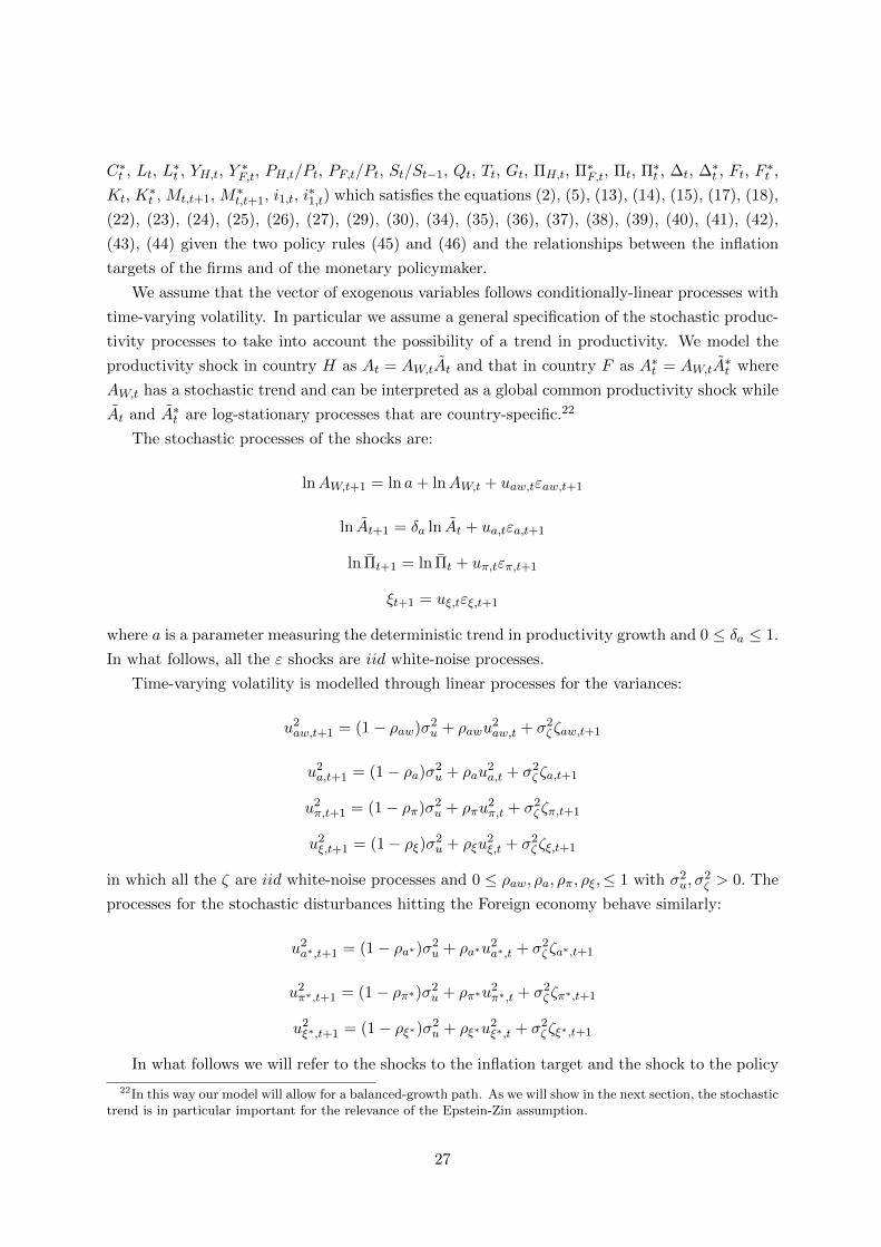
We assume that the vector of exogenous variables follows conditionally-linear processes with

time-varying volatility. In particular we assume a general specification of the stochastic produc-

tivity processes to take into account the possibility of a trend in productivity. We model the

productivity shock in country H as At = AW,tAt and that in country F as A∗t = AW,tA∗t where

AW,t has a stochastic trend and can be interpreted as a global common productivity shock while

At and A∗t are log-stationary processes that are country-specific.22

The stochastic processes of the shocks are:

lnAW,t+1 = ln a+ lnAW,t + uaw,tεaw,t+1

ln At+1 = δa ln At + ua,tεa,t+1

ln Πt+1 = ln Πt + uπ,tεπ,t+1

ξt+1 = uξ,tεξ,t+1

where a is a parameter measuring the deterministic trend in productivity growth and 0 ≤ δa ≤ 1.

In what follows, all the ε shocks are iid white-noise processes.

Time-varying volatility is modelled through linear processes for the variances:

u2aw,t+1 = (1− ρaw)σ2

u + ρawu2aw,t + σ2

ζζaw,t+1

u2a,t+1 = (1− ρa)σ2

u + ρau2a,t + σ2

ζζa,t+1

u2π,t+1 = (1− ρπ)σ2

u + ρπu2π,t + σ2

ζζπ,t+1

u2ξ,t+1 = (1− ρξ)σ2

u + ρξu2ξ,t + σ2

ζζξ,t+1

in which all the ζ are iid white-noise processes and 0 ≤ ρaw, ρa, ρπ, ρξ,≤ 1 with σ2u, σ

2ζ > 0. The

processes for the stochastic disturbances hitting the Foreign economy behave similarly:

u2a∗,t+1 = (1− ρa∗)σ2

u + ρa∗u2a∗,t + σ2

ζζa∗,t+1

u2π∗,t+1 = (1− ρπ∗)σ2

u + ρπ∗u2π∗,t + σ2

ζζπ∗,t+1

u2ξ∗,t+1 = (1− ρξ∗)σ2

u + ρξ∗u2ξ∗,t + σ2

ζζξ∗,t+1

In what follows we will refer to the shocks to the inflation target and the shock to the policy

22In this way our model will allow for a balanced-growth path. As we will show in the next section, the stochastictrend is in particular important for the relevance of the Epstein-Zin assumption.

27

instruments as monetary or nominal shocks while the productivity shock will be the real shock.

4.5 Solution

Given the above specification for the processes of the exogenous state variable, we can write

them more compactly as

zt+1 = Λzzt + ηt+1 (47)

where the vector zt is defined as zt ≡ [(∆ lnAW,t− ln a), ln At, ξt, ln ΠH,t, ln A∗t , ξ∗t , ln Π∗F,t]

′ and

Λz is an appropriately-defined square matrix. The vector ηt+1 is given by

ηt+1 = Utεz,t+1 (48)

where εz,t+1 collects the innovations, which are assumed to have a bounded support and to

be independently and identically distributed with mean zero and variance/covariance matrix

Iz, where Iz is an identity matrix of the same dimension of the vector z; Ut is a diagonal

matrix whose elements on the diagonal are collected into a vector ut. In particular ut follows

the exogenous stochastic linear process given by

u2t+1 = σ2

u(Iz − Λu)u2 + Λuu2t + σ2

ζZζu,t+1. (49)

Each element of u2t is the corresponding squared value of each element of ut, which still cor-

responds to the diagonal of matrix Ut as in (48); u2 is a vector of steady-state variances, Z

and Λu are appropriately defined square matrices; ζu,t+1 is a vector of innovation collecting the

above ζ which are assumed to have a bounded support and to be independently and identi-

cally distributed with mean zero and variance/covariance matrix Iz; σu and σζ are scalars with

σu, σζ ≥ 0.

Noticing that (47) with (48) and (49) defines a conditionally-linear process, we can write the

set of equilibrium conditions of the model together with the conditional expectation of (47) in

a more compact form

Et {f(yt+1, xt+1, yt, xt)} = 0, (50)

for an appropriately defined vector of function f(·) where yt identifies the non-predetermined

variables while the vector xt of state variables contains also the vector of exogenous predeter-

mined variables zt. Given the processes (47), with (48) and (49), an equilibrium of our model is a

sequence for the vector of endogenous non-predetermined variables yt and for the state variables

xt that satisfies (50), given the initial conditions.

Benigno et al. (2010) characterize the solution of the above model and show that a first-order

approximation of the solution can be written as

yt = gxxt,

28

xt+1 = hxxt + hηηt+1,

for appropriately-defined matrices gx, hx and hη. This approximation does not correspond to a

fully linear solution since ηt+1, defined, in (48) is non-linear. However, it is the best condition-

ally linear approximation and, in particular, the matrices gx and hx coincide with those of a

fully linear approximation. Our first-order approximation maintains heteroskedastic shocks but

time-varying volatility does not play a distinct role, meaning that the impulse response of the

endogenous variables with respect to the shock to volatility, ζu,t+1, is always zero. The advan-

tage of performing a conditionally-linear approximation instead of a fully-linear approximation,

in which ηt+1 is also linearized, is clear when we look at a second-order approximation of the

solution. Benigno et al. (2010) show that this takes the form

yt = gxxt +1

2(Iy ⊗ x′t)gxxxt +

1

2guuu

2t +

1

2gzzσ

2u, (51)

xt+1 = hxxt +1

2(Ix ⊗ x′t)hxxxt +

1

2huuu

2t +

1

2hzzσ

2u + hηηt+1, (52)

for appropriately defined matrices gxx, gzz, guu and hxx, hzz, huu. In this second-order approxi-

mation, the volatility of the exogenous state variables now plays a distinct and direct role through

the matrices guu and huu. Indeed the endogenous variables are now in a linear relationship with

the vector of volatilities, u2t . Other methods discussed in the literature, as Fernandez-Villaverde

et al. (2010), need instead to rely at least on a third-order approximation to get such a distinct

role for volatilities in influencing the endogenous variables.

The second advantage of our conditionally-linear approximation is that risk premia, evaluated

using a first-order approximation of the model, will be also time-varying. This feature enables

the model to characterize some stylized facts on the role of volatility on international data in a

simple way.

5 Exchange rates and risk: a simple example

In this section, before we turn to the solution of our general model, we present a simplified

framework to study whether we can already account for some of the facts that we have under-

lined in the empirical analysis. The framework of this section, with its analytical solutions, will

be also helpful to explain how our solution method works and represent a useful benchmark

through which we can later evaluate the effects of relaxing the assumptions of this section. The

simplifying assumptions are: 1) monetary policy in each country is modeled through Taylor

rules reacting only to the domestic CPI inflation rate with the same coefficients across coun-

tries, later in the section we allow for interest-rate smoothing; 2) purchasing power parity holds

(v = v∗ = n) 3) flexible prices (α = α∗ = 0) and constant real rates which make real shocks

irrelevant for the analysis of this section. Therefore, we will abstract completely from produc-

tivity shocks and give just a monetary explanation of the facts related to the nominal exchange

29

rate and the UIP deviations.

The starting points are the standard arbitrage-free conditions (26) and (27). As discussed

more generally in Benigno et al. (2010), we rely on approximation methods to solve our model.

In particular we show that it is sufficient to use a second-order approximation of the model to

characterize how risk influences the variables of interest and in particular the exchange rate.

By taking a second-order approximation of (26) and (27), we obtain

ıt = −EtMt+1 −1

2V artMt+1 (53)

ı∗t = −EtM∗t+1 −1

2V artM

∗t+1 (54)

where hats denote log-deviations with respect to the steady state, in which we assume i = i∗ =

1/β− 1, and Et and V art are conditional expectation and variance operators, respectively.23 In

logs, the complete-market assumption (19) implies

Mt+1 = M∗t+1 −∆st+1. (55)

We can combine (53), (54) and (55) to write the short-term excess return of investing in the

currency of country F with respect to investing in the currency of country H as

ı∗t + Et∆st+1 − ıt =ϑ∗t2− ϑt

2(56)

where

ϑt = covt(Mt+1,∆st+1) ϑ∗t = covt(M∗t+1,−∆st+1). (57)

The intuition for why there can be or cannot be an excess return on foreign currency with

respect to domestic currency depends on whether foreign currency is or is not a bad hedge with

respect to risk relatively to domestic currency. The standard principle is that an asset is ”risky”

when it does not pay well when money is really needed. In this case, investors command a

premium to hold it which shows up in an excess return relatively to other assets. In our context,

the stochastic discount factors measure the agents’ appetites for state contingent wealth and

therefore when money is needed or not. When Mt+1 and M∗t+1 are high in some contingencies,

the appetites for wealth of the Home and Foreign agents are also high in those contingencies.

An asset that pays well under this case is a good asset and represents a good hedge with respect

to risk. If, for example, the currency of country H depreciates (the nominal exchange rate

depreciates, i.e. ∆st+1 > 0) then having invested in the currency of country F is indeed a good

23Notice that (53) and (54) do not hold exactly but up to residuals which are of third-order in an appropriatenorm on the stochastic disturbances. Under the assumption of log-normality, as in Backus et al. (2010), theywould hold exactly.Our analysis is a local analysis and their is a global analysis. Therefore, their approachis limited to the possibility of a closed-form solution. Moreover, the two frameworks will also deliver subtledifferences in terms of the conditions needed for the determinancy of the equilibrium.

30

investment since it delivers more money when it is really needed. In this case ϑt is positive and

ϑ∗t is negative. In general, the expected short-term excess return of investing in the currency of

country F with respect to that of investing in the currency of country H is negative because

simply the currency of country H is not a good hedge with respect to the appetite for wealth of

both agents. In general, to have a negative expected excess return on the Foreign-versus-Home

currency it is not necessary that ϑt should be positive and ϑ∗t negative, but just ϑt > ϑ∗t .

Finally, it is worth stressing that the right-hand side of equation (56) captures the deviations

from uncovered interest parity in any model in which no-arbitrage restrictions apply. Indeed, so

far, none of the simplifying assumptions 1), 2) and 3) has been used.

5.1 Simple Taylor Rules

By making assumption 1) (φi = φ∗i = φy = φ∗y = φs = φ∗s = 0, φπ = φ∗π with interest

rate reacting to CPI inflation into (45) and (46)), we can further use (56) to determine the

equilibrium nominal exchange rate. In particular, the short-term nominal interest rates follow

simple Taylor rules in which

ıt = πt + φπ(πt − πt) + ξt (58)

ı∗t = π∗t + φπ(π∗t − π∗t ) + ξ∗t (59)

where πt and π∗t represent the logs of Home and Foreign inflation-target shocks and ξt and ξ∗t

are the Home and Foreign policy shocks as in (45) and (46).

We now use the simplifying assumption 2), that there is no home bias in consumption

implying that purchasing power parity holds, i.e. πt = π∗t + ∆st.

5.1.1 Exchange rate determination

Using PPP and rules (58) and (59) into (56) we obtain a first-order stochastic difference equation

in ∆st

Et∆st+1 = φπ∆st + (1− φπ)(πt − π∗t ) + (ξt − ξ∗t )− 1

2(ϑt − ϑ∗t )

which can be solved forward to deliver a unique bounded solution for the nominal exchange rate

of the form

∆st = Et

∞∑T=t

(1

φπ

)T+1−t [(φπ − 1)(πT − π∗T )− (ξT − ξ∗T ) +

1

2(ϑT − ϑ∗T )

], (60)

under the requirement, for determinacy, that the Taylor’s principle holds, i.e. φπ > 1.24

There are several implications of the above simple model for nominal exchange rate determi-

nation. First, the design of the monetary policy rules is important. Indeed, equation (60) holds

24Necessary and sufficient conditions for the local determinancy of equilibrium are discussed more extensivelyin Benigno and Benigno (2008), for two-country open-economy models.

31

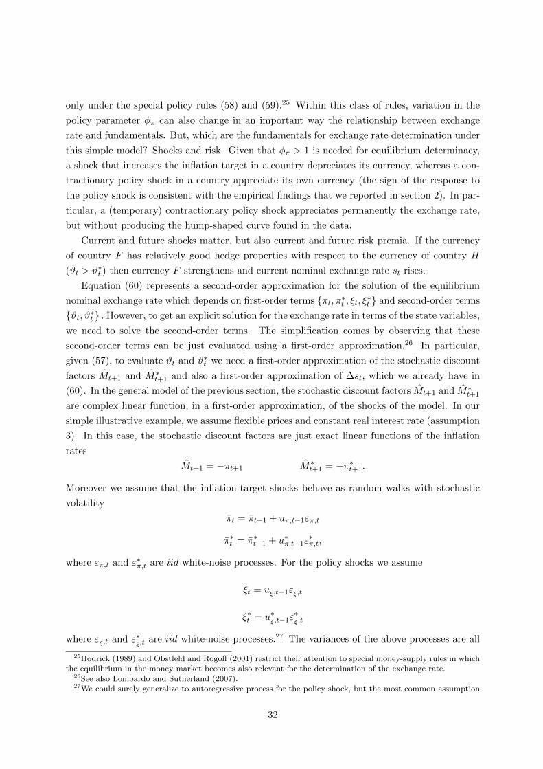
only under the special policy rules (58) and (59).25 Within this class of rules, variation in the

policy parameter φπ can also change in an important way the relationship between exchange

rate and fundamentals. But, which are the fundamentals for exchange rate determination under

this simple model? Shocks and risk. Given that φπ > 1 is needed for equilibrium determinacy,

a shock that increases the inflation target in a country depreciates its currency, whereas a con-

tractionary policy shock in a country appreciate its own currency (the sign of the response to

the policy shock is consistent with the empirical findings that we reported in section 2). In par-

ticular, a (temporary) contractionary policy shock appreciates permanently the exchange rate,

but without producing the hump-shaped curve found in the data.

Current and future shocks matter, but also current and future risk premia. If the currency

of country F has relatively good hedge properties with respect to the currency of country H

(ϑt > ϑ∗t ) then currency F strengthens and current nominal exchange rate st rises.

Equation (60) represents a second-order approximation for the solution of the equilibrium

nominal exchange rate which depends on first-order terms {πt, π∗t , ξt, ξ∗t } and second-order terms

{ϑt, ϑ∗t } . However, to get an explicit solution for the exchange rate in terms of the state variables,

we need to solve the second-order terms. The simplification comes by observing that these

second-order terms can be just evaluated using a first-order approximation.26 In particular,

given (57), to evaluate ϑt and ϑ∗t we need a first-order approximation of the stochastic discount

factors Mt+1 and M∗t+1 and also a first-order approximation of ∆st, which we already have in

(60). In the general model of the previous section, the stochastic discount factors Mt+1 and M∗t+1

are complex linear function, in a first-order approximation, of the shocks of the model. In our

simple illustrative example, we assume flexible prices and constant real interest rate (assumption

3). In this case, the stochastic discount factors are just exact linear functions of the inflation

rates

Mt+1 = −πt+1 M∗t+1 = −π∗t+1.

Moreover we assume that the inflation-target shocks behave as random walks with stochastic

volatility

πt = πt−1 + uπ,t−1επ,t

π∗t = π∗t−1 + u∗π,t−1ε∗π,t,

where επ,t and ε∗π,t are iid white-noise processes. For the policy shocks we assume

ξt = uξ,t−1εξ,t

ξ∗t = u∗ξ,t−1ε

∗ξ,t

where εξ,t and ε∗

ξ,tare iid white-noise processes.27 The variances of the above processes are all

25Hodrick (1989) and Obstfeld and Rogoff (2001) restrict their attention to special money-supply rules in whichthe equilibrium in the money market becomes also relevant for the determination of the exchange rate.

26See also Lombardo and Sutherland (2007).27We could surely generalize to autoregressive process for the policy shock, but the most common assumption

32

time varying following the linear stochastic processes

u2π,t = σ2

u + ρπ(u2π,t−1 − σ2

u) + σ2ζζπ,t

u∗2π,t = σ2u + ρπ(u∗2π,t−1 − σ2

u) + σ2ζζ∗π,t

u2ξ,t = σ2

u + ρξ(u2ξ,t−1 − σ2

u) + σ2ζζξ,t

u∗2ξ,t = σ2u + ρξ(u

∗2ξ,t−1 − σ2

u) + σ2ζζ∗ξ,t,

where 0 ≤ ρπ, ρξ ≤ 1 and all the zetas are iid white-noise processes while σ2u and σ2

ζ are non-

negative parameters.

Given the above defined processes, and up to a first-order approximation, equation (60)

implies

∆st = (πt − π∗t )−1

φπ(ξt − ξ∗t ) (61)

where movements in the inflation-target shocks move one-to-one the nominal exchange rate,

while the response of the nominal exchange rate to policy shocks depends on the parameter of

the Taylor rules. Using (53) and (58), and (54) and (59) respectively, we can determine the

domestic and foreign inflation rates as

πt = πt −1

φπξt (62)

π∗t = π∗t −1

φπξ∗t (63)

which in this simple example only reflect the influence of their own monetary shocks. We can

use (61), (62) and (63) to evaluate the risk premia component in (57)

ϑt = covt(Mt+1,∆st+1) = −u2π,t −

1

φ2π

u2ξ,t

ϑ∗t = covt(M∗t+1,−∆st+1) = −u∗2π,t −

1

φ2π

u∗2ξ,t

which can be plugged into (60) to obtain the equilibrium exchange rate

∆st = (πt − π∗t )−1

φπ(ξt − ξ∗t )− 1

2

1

φπ − ρπ(u2π,t − u∗2π,t)

−1

2

1

φπ − ρξ1

φ2π

(u2ξ,t − u∗2ξ,t). (64)

In this solution, the time-varying volatilities of the monetary shocks matter for the determination

of the nominal exchange rate.28 This is the important consequence of the solution method

in the literature is that of white-noise processes.28Notice that the terms in σ2

u cancel out because of the symmetry assumed.

33

proposed by Benigno et al. (2010) in which a second-order approximation of the model is

sufficient to get a distinct role for time-varying uncertainty in affecting the determination of

variables of interest. In (64), the higher the variance of the inflation-target and of the policy

shocks in country H, the stronger the currency of country H is. And specularly for the volatility

of the monetary shocks in country F . These theoretical findings are in part consistent with the

empirical results of Section 2: there, we reported that an increase in both volatilities leads to

an appreciation of the currency (at least in the medium-run with the exception of the USD/Yen

bilateral).

The model is then consistent with the view that more uncertainty can be good for the nominal

exchange rate, meaning that the exchange rate can even appreciate when volatility rises. The

intuition insists on the good or bad hedging properties of the currency. If a currency is a good

hedge with respect to a particular risk and this risk increases, then there is more demand of

the currency and its exchange rate appreciates. For example, when the Home inflation target

shock falls the appetite for wealth for the Home consumers rises. At the same time the nominal

exchange rate appreciates, therefore Home currency delivers more money when needed, relatively

to foreign currency. This is good for hedging purposes. When the variance of the Home inflation-

target shock rises, the good hedging properties of Home currency are enhanced and therefore

the higher demand of Home currency leads to an appreciation.

The magnitude of the effects on the exchange rate depends obviously on the magnitude of

the shock but also on the persistence. The higher the persistence the higher the response. It

is further influenced by the policy parameter of the Taylor rule, the higher φπ the muted the

response of the exchange rate. In this symmetric example, as for the primitive shocks, what

matters for the determination of the equilibrium exchange rate is the relative strength between

the volatilities of the monetary shocks across countries. However, while a positive inflation-

target shock and a positive policy shock produce responses of opposite sign on the equilibrium

nominal exchange rate, an increase in the volatility of the inflation-target shock or of the policy

shock impacts in the same direction.

5.1.2 UIP implications

ı∗t + Et∆st+1 − ıt =1

2

(u2π,t − u∗2π,t

)+

1

2φ2π

(u2ξ,t − u∗2ξ,t

)The expected excess return of investing in the currency of country F with respect to that

of country H rises with the increase in the volatilities of the monetary shocks in country H.

Consistently with the discussion of the previous section, a rise in the volatility of both the

monetary shocks in country H enhance the hedging properties of currency H and reduces those

of currency F. Currency F requires a premium to be held. While the response of the foreign

excess return to an increase in volatility of monetary-policy shock (u2ξ,t) is, at first pass, consistent

with the empirical findings in Section 2, an increase in the volatility of the inflation-target shock

(u2π,t) goes in the opposite direction with what we found in the data.

34

This is not the only counterfactual result of this section. As discussed in Backus et al.

(2010), this stylized framework cannot account for the negative slope coefficient in the UIP

regression: the regression of the one-period changes in the nominal exchange rate on the interest

rate differential. Using (64), and analogous solutions for the interest rates in the two countries,

the coefficient of the UIP regression implied by our model would be

βuip =Cov(∆st+1, ıt − ı∗t )

V ar(ıt − ı∗t )

βuip =var(πt − π∗t ) + a2

1,uπρπφπvar(u2

π,t − u∗2π,t) + a21,uξ

ρξφπvar(u2

ξ,t − u∗2ξ,t)var(πt − π∗t ) + a2

1,uπvar(u2

π,t − u∗2π,t) + a21,uξ

var(u2ξ,t − u∗2ξ,t)

where the assumption of a unit-root processes for the inflation-target shocks blows up numerator

and denominator, in large samples, to produce a unitary coefficient. However, abstracting from

this issue or focusing on small samples, the only possibility for βuip to be negative is that ρξ/φπ

be negative, as shown in Backus et al. (2010). Since assuming ρξ < 0 is not plausible, then in

our simplified framework βuip is positive and decreasing with φπ, the inflation’s coefficient in

the Taylor rule.

5.2 Taylor rules with interest rate smoothing

One natural extension to the previous setting is to consider a model in which the interest rate set

by the policy authority moves gradually (interest rates are smoothed over time as in McCallum,

1994, and Backus et al., 2010) so that interest rates depend also on their past value. The

modified Taylor’s rules take the form

ıt = φiıt−1 + (1− φi)[πt + φπ(πt − πt)] + ξt,

ı∗t = φiı∗t−1 + (1− φi)[π∗t + φπ(π∗t − π∗t )] + ξ∗t ,

to replace (58) and (59). Following the same steps as before, it is possible to show that the

equilibrium exchange rate is given by

∆st = − φiλ− φi

(ıt−1 − ı∗t−1) +λ

λ− φi(πt − π∗t )−

1

λ(ξt − ξ∗t )

−1

2

1

λ− ρu

(λ

λ− φi

)2

(u2π,t − u∗2π,t)−

1

2

1

λ− ρu1

λ2(u2ξ,t − u∗2ξ,t). (65)

where we are restricting φi to be 0 < φi < 1 and where λ ≡ φπ(1−φi)+φi with the requirement

λ > 1 for equilibrium determinacy implying again φπ > 1. In general allowing for interest-rate

smoothing changes also the short-run responses to the shocks and the volatilities but does not

change the sign of the response. Responses are obviously changed at longer horizons given the

lagged reaction to the interest rate.

The important contribution of assuming interest-rate smoothing is that the negative depen-

35

dence on lagged interest rates can be such to reduce the coefficient of the UIP regression and

eventually to turn it negative, as discussed in Backus et al. (2010). However, it does not change

the sign of the responses of the expected excess return on foreign-versus-domestic currency to

the volatilities of the monetary shocks.

6 Exchange rates and risk: the general case

We now turn to the implications of the more general framework with sticky prices presented in

Section 4. First, we investigate the properties of the nominal stochastic discount factor which,

as shown in the previous section, is critical to understand the relationship between exchange

rate and risk, and to evaluate the risk premia embedded in asset prices.

In our general framework the stochastic discount factor depends on the Epstein-Zin prefer-

ence specification. Our first result shows a peculiarity of Epstein-Zin preferences in an interna-

tional context. In closed economy, a standard finding is the irrelevance of Epstein-Zin preferences

for quantities and the importance for asset pricing.29 The irrelevance result can be understood

by observing that up to a first-order approximation, Epstein-Zin preferences do not matter for

the equilibrium allocation. In contrast, we will show that Epstein-Zin preferences might be also

important for quantities, in our two-country open-economy model, since, as shown in equation

(30), the cross-country surprises in utility affect the international distribution of wealth. Indeed

in a first-order approximation, we obtain

Gt+1 = Gt + (γ − ρ)[(Vt+1 − EtVt+1)− (V ∗t+1 − EtV ∗t+1)].

where hats denote log-deviations with respect to the steady state. Under expected utility,

ρ = γ, Gt will be constant across time, implying the standard risk-sharing condition which links

marginal utilities of nominal income across countries. Instead, with the Epstein-Zin preferences,

the cross-country differences in the realization of utility matter for the distribution of wealth.

This might have interesting consequences for the equilibrium allocation of quantities.30

However, the general-equilibrium flavor of our analysis makes it difficult to keep track of all

the effects through analytical solutions. To get further insights and to study the contribution

of the Epstein-Zin preferences to the evaluation of risk premia, we now discuss more deeply

the properties of the stochastic discount factor. In a first order approximation of (22), the

Home-country nominal discount factor can be written as

Mt,t+1 = −(γ−ρ)(Vt+1−EtVt+1)+(1−ρ)(1−ψ)∆Lt+1−[1−ψ(1−ρ)](∆Ct+1 +∆AW,t+1)−πt+1,

(66)

where we have defined Lt = ln(1−Lt)/ ln(1−L) while Ct denotes the deviations of detrended con-

29See among others Rudebush and Swanson (2009).30Notice however that in this first-order approximation EtGt+1 = Gt and therefore Gt is a local martingale.

36

sumption with respect to the steady state, Ct ≡ lnCt/AW,t− ln(C/AW ).31 Under the expected-

utility model, γ = ρ, the stochastic discount factor is a function of consumption growth, which

can be decomposed in the growth of detrended consumption and in the growth of world produc-

tivity, a function of the CPI inflation rate and of the growth in hours worked. An increase in

consumption lowers the stochastic discount factor and the appetite for wealth, for realistic val-

ues of the intertemporal elasticity of substitution, ρ. The impact of the growth in hours worked

depends on ρ ≶ 1 while an increase in the inflation rate reduces instead unambiguously the

appetite for wealth. On top of affecting the equilibrium allocation and therefore the allocation

of consumption and labor, as discussed above, Epstein-Zin preferences bring the novelty that

also surprises in the indirect utility matter through the term (Vt+1 − EtVt+1). To get further

insights on this component, we take a first-order approximation of the indirect utility (2) and

show that we can relate it to the present discounted value of the surprises in consumption and

labor

Vt+1 − EtVt+1 = (1− β)

∞∑T=t+1

βT−t−1[∆Et+1(ψ(CT + AW,T ) + (1− ψ)LT )].

where we have defined ∆Et+1(·) = Et+1(·) − Et(·). In general equilibrium, interaction terms

will be quite complex. However, at the cost of losing generality, we can get further insights by

looking at a limiting case in which the discount factor, β, is close to the unitary value. In this

case, indeed, we show that Epstein-Zin preferences do not matter for the equilibrium allocation

of quantities, up to a first-order approximation. Under the assumption β −→ 1 we can write

Vt+1 − EtVt+1 ≈ ∆Et+1(ψ(C∞ + AW,∞) + (1− ψ)L∞),

which shows that only the stochastic trend in the respective variables influences the current

surprises in utility. However, since C and L are respectively a detrended and a stationary

variable, their stochastic trends are zero. The surprises to indirect utility will therefore only

depend on the stochastic trend in world productivity

Vt+1 − EtVt+1 ≈ ψ∆Et+1(AW,∞) = ψua,tεa,t+1,

which displays also time-varying risk. The importance of this factor in (66) will be higher,

the larger the difference between γ and ρ. Under this particular case, the ability of Epstein-

Zin preferences to explain risk premia hinges upon the comovements between returns and the

nominal stochastic discount factor. In particular when agents have a preference for an early

resolution of uncertainty, i.e. γ > ρ, a negative shock to world productivity εa,t implies bad

news with respect to long-run consumption which are reflected in bad news on utility. In this

case, the stochastic discount factor rises and the appetite for state contingent wealth too. This

mechanism would apply also to the country F . Indeed, it is also true that the surprise in

the utility of the foreign country depends on the shifts in the long-run component of world

31The balance growth path of the model is defined with respect to the common trend in productivity, AW .

37

productivity

V ∗t+1 − EtV ∗t+1 ≈ ψ∆Et+1(AW,∞) = ua,tεa,t+1.

Under the case β −→ 1, Epstein-Zin preferences might therefore contribute to imply highly

correlated discount factors across countries and deliver a global explanation for the risk premia,

which will be time-varying and driven by the shocks to the common technological process. The

consequence of this result is indeed that, up to a first-order approximation, general equilibrium

effects will be shut down. Since surprises in the utility of the Home and Foreign country are

highly correlated then, using (29) and (30), Gt is approximately constant over time32

Gt+1 = Gt + (γ − ρ)[(Vt+1 − EtVt+1)− (V ∗t+1 − EtV ∗t+1)]

≈ Gt.

This is true up to a first-order approximation, but not in a second-order approximation where

it might be possible that EZ preferences have sizeable effects also on quantities.

6.1 Quantitative Evaluation

We now move to a quantitative evaluation of the model implications. In particular, a second-

order approximation of the model will be relevant to study the relationship between risk and

the exchange rate, and provide a quantitative assessment of such links. This will be implicit in

the general solution of the nominal and real exchange rate

∆St = gsxxt +1

2x′tg

sxxxt +

1

2gsuuu

2t +

1

2gszzσ

2u

Qt = gqxxt +1

2x′tg

qxxxt +

1

2gquuu

2t +

1

2gqzzσ

2u

where the index i = s, q selects appropriate elements of the respective vector or matrices. In this

solution, time-varying uncertainty for the stochastic disturbances of the model affects linearly

the nominal and real exchange rates through the factors giuu.

6.1.1 Calibration

In this section we describe our baseline calibration for the general model. The strategy that we

adopt for the calibration exercise is to rely as much as possible on a standard values for the

parameters and conduct a sensitivity analysis on those for which there are divergences in the

literature. We assume that the Home and Foreign economy are of equal size and are calibrated

in a symmetric fashion. In this calibration section we think about our two-country world as

U.S. versus the Euro area abstracting then from asymmetries that might be important for

32The statement is true under the assumption that β is close to the unitary value, up to a first-order approxi-mation and independently of the values assumed by the parameters γ and ρ.

38

understanding some empirical regularities when it comes to small open economies.33

In choosing the parameters of utility function, we set β to 0.994 consistent with other studies

with Epstein-Zin preferences (e.g. Fernandez-Villaverde et al., 2010). We set the inverse of the

intertemporal elasticity of substitution ρ to 2, implying an intertemporal elasticity of substitution

(IES) in consumption of 0.5, which is consistent with estimates in the micro literature (e.g.,

Vissing-Jorgensen, 2002) and used also in the international real business cycle literature as in

Stockman and Tesar (1995). We set the coefficient of relative risk aversion γ to 5 as in Backus

et al. (2010). We set the share of consumption in the utility bundle, ψ, to 1/3 as in Cooley and

Prescott (1995) in order to imply that in the steady state households devote one-third of their

time to work.

We calibrate the parameters pertaining to the consumption basket in the following way. The

share of home goods in tradable consumption, ν, is set to 0.87. The elasticity of substitution

between home and foreign traded goods, θ, is assumed equal to 1.5 which is in the range of the

plausible values.

We set the firms’ output elasticity with respect to labor, ϕ, to 2/3, and the elasticity of

substitution among differentiated goods, σ, to 6 (implying a steady state markup of 20%) and

α = 0.66 and α∗ = 0.75 implying an average length of price contracts equal to 3 and 4 quarters,

respectively; all these are standard in the literature and consistent with the posterior estimates

for the U.S. and Euro area by Lubik and Schorfeide (2005).

Regarding the policy rules we assume φi = 0.76 , φπ = 1.41, φs = 0.03 and φy = .66 for

the U.S. economy and φ∗i = 0.84, φ∗π = 1.37, φ∗s = 0.03 and φ∗y = 1.27 for the Euro area that

corresponds to the posterior estimates that Lubik and Schorfeide (2005) have found for the U.S.

and Euro area respectively.34

We now turn to the calibration of the stochastic processes. For the productivity shocks we

use the posterior estimates of Lubik and Schorfeide (2005) for the U.S. and Euro-area: δA = 0.83,

δ∗A = 0.85 with σA = 1.66 and σ∗A = 2.71 as the values through which we scale the individual

standard deviation for the home and foreign shocks respectively. We assume no persistence for

the policy shocks and we scale its standard deviation by σξ = 0.18 for both countries based

on the estimates of Lubik and Schorfeide (2005). For the inflation-target shocks we follow

Ireland (2007) and set it to σπ = 0.1. For the persistence of the volatility shocks, we calibrate

the autocorrelation coefficients at the values implied by fitting an AR(1) process for each of the

three time-series employed in the empirical part. As a consequence, we set ρaw = ρa = ρa∗ = .71,

ρπ = ρπ∗ = .67 and ρξ = ρξ∗ = .53.

33Relevant asymmetries could be in terms of a policy rule that reacts to exchange rate for small open economiesor different degree of openess that affect critically the international transmission mechanism of shocks.

34Although we specified a theoretical model in which monetary-policy credibility might possibly play a role, wedisregard this role in the present work, and accordingly parameterize κ = κ∗ = 1.

39

0 5 10 150.6

0.4

0.2

0

0.2 RER

0 5 10 150.05

0

0.05

0.1

0.15 r r*

0 5 10 150

0.01

0.02

0.03

0.04 Real UIP

0 5 10 150.3

0.2

0.1

0

0.1 NEX

0 5 10 150.06

0.04

0.02

0

0.02 i i*

0 5 10 150

0.05

0.1 Nominal UIP

0 5 10 151

0.5

0 YH

0 5 10 150.1

0

0.1

0.2

0.3 H

0 5 10 150.04

0.02

0

0.02 i

Figure 10: Dynamic responses to a monetary-policy volatility shock (innovation to the volatility of the monetarypolicy instrument). The panels show: real exchange rate (RER), real interest rate differential (r− r∗), deviationsfrom Real UIP, nominal exchange rate (NEX), nominal interest rate differential (i− i∗), deviations from NominalUIP, domestic output (YH), domestic inflation (πH), domestic short-term nominal interest rate (i).

6.1.2 Results

In this Section we evaluate to what extent our two-country model with recursive preferences and

stochastic volatility can replicate the dynamic properties of the data found in Sections 2 and 3.

Our analysis is mainly qualitative as we compare our model-based impulse response with the

ones generated by the VAR. In what follows, we plot impulse response of the main variables of

interest: real exchange rate (RER), real interest rate differential (r − r∗), deviations from real

uncovered interest-rate parity (Real UIP), nominal exchange rate (NEX), nominal interest rate

differential (i− i∗), nominal uncovered interest-rate parity (Nominal UIP), and domestic output

(YH), producer inflation (πH) and Home nominal interest rate (i).35

In particular, we identified two main regularities on the relationship between exchange rate

and risk: (i) an increase in the volatility of both monetary-policy and inflation-target shocks

appreciates the exchange rate, while an increase in the volatility of the productivity shock

induces an exchange rate depreciation; (ii) an increase in the volatility of the monetary-policy

shock leads to deviations from UIP in the form of an increase in the excess return on foreign-

versus-domestic currency while an increase in the volatility of the inflation-target shock leads to

a fall in the excess return.

An additional regularity, originally documented by Eichenbaum and Evans (1995) and that

we also confirm by controlling for the effects of time-varying volatility, is that a contractionary

monetary-policy shock produces a persistent appreciation of the exchange rate and persistent

deviations from the UIP in the form of positive excess returns on domestic securities.

Figures 10 and 11 display the dynamic response of our variables of interest to volatility

35For ease of comparison with the empirical analysis, we normalize the size of each shock to the one featuredin the VAR analysis.

40

0 5 10 150.2

0.1

0

0.1

0.2 RER

0 5 10 150

0.01

0.02

0.03 r r*

0 5 10 150

0.005

0.01

0.015 Real UIP

0 5 10 150.4

0.3

0.2

0.1

0 NEX

0 5 10 150.06

0.04

0.02

0

0.02 i i*

0 5 10 150

0.02

0.04

0.06

0.08 Nominal UIP

0 5 10 150.8

0.6

0.4

0.2

0 YH

0 5 10 150.02

0

0.02

0.04

0.06 H

0 5 10 150.06

0.04

0.02

0

0.02 i

Figure 11: Dynamic responses to an inflation-target volatility shock (innovation to the volatility of the inflationtarget). The panels show: real exchange rate (RER), real interest rate differential (r − r∗), deviations from RealUIP, nominal exchange rate (NEX), nominal interest rate differential (i − i∗), deviations from Nominal UIP,domestic output (YH), domestic inflation (πH), domestic short-term nominal interest rate (i).

shocks hitting the monetary-policy instrument and the inflation target, respectively. The figures

show that the model is indeed able to imply an appreciation of the real exchange rate and

deviations from the UIP in the form of positive excess returns from investing in foreign-currency

denominated bonds, consistently with our empirical findings both in real and in nominal terms.

A rise in home nominal volatility tends also to reduce domestic output and increase domestic

producer inflation while the domestic nominal interest rate declines, proportionately more than

the foreign one. An interesting difference among the two nominal shocks arises in the response

of the real interest rate differential. In the case of the shock to volatility of the inflation target,

the real interest rate differential is positive on impact and increasing in the short run while

it is negative on impact following a shock to the volatility of the monetary instrument. This

difference arises because the volatility shock to the monetary instrument generates more inflation

than the shock to the inflation target.

Figure 12, similarly shows the dynamic response of Real Exchange Rate and the deviation

from UIP to a volatility shock hitting global productivity. The asymmetries in the degrees of

price stickiness and the response coefficients of the policy rules imply that innovations in the

level and/or volatility of the global productivity shocks are able to produce a non-zero response

on international variables. In particular, in response to an increase in the volatility of the global

productivity shock, the RER depreciates and we observe positive deviations from nominal UIP

consistent with the sign of the response that we observe in our empirical findings. However, the

nominal exchange rate appreciates on impact. Therefore, the movements in the real exchange

rate are mainly driven by changes in domestic CPI inflation.

All these results are qualitatively consistent with the empirical regularities Fact 1 and 2, and

also show that our approximation method is effective to study the link between time-varying

41

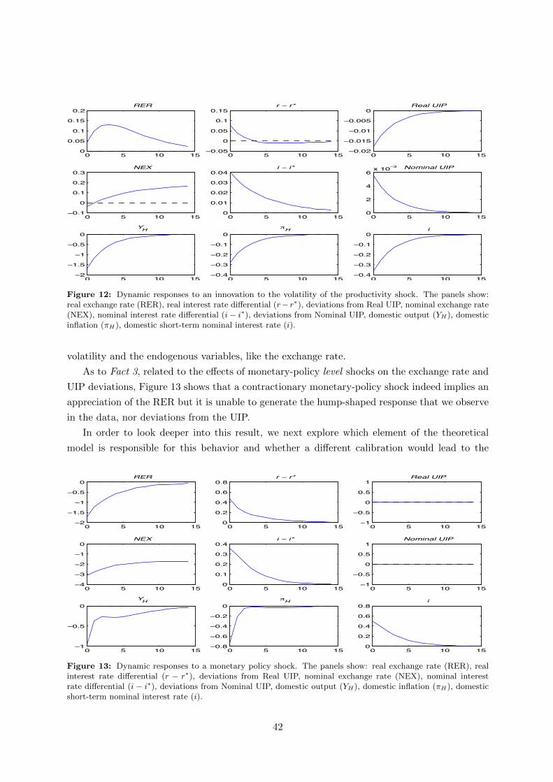
0 5 10 150

0.05

0.1

0.15

0.2 RER

0 5 10 150.05

0

0.05

0.1

0.15 r r*

0 5 10 150.02

0.015

0.01

0.005

0 Real UIP

0 5 10 150.1

0

0.1

0.2

0.3 NEX

0 5 10 150

0.01

0.02

0.03

0.04 i i*

0 5 10 150

2

4

6x 10 3 Nominal UIP

0 5 10 152

1.5

1

0.5

0 YH

0 5 10 150.4

0.3

0.2

0.1

0 H

0 5 10 150.4

0.3

0.2

0.1

0 i

Figure 12: Dynamic responses to an innovation to the volatility of the productivity shock. The panels show:real exchange rate (RER), real interest rate differential (r− r∗), deviations from Real UIP, nominal exchange rate(NEX), nominal interest rate differential (i− i∗), deviations from Nominal UIP, domestic output (YH), domesticinflation (πH), domestic short-term nominal interest rate (i).

volatility and the endogenous variables, like the exchange rate.

As to Fact 3, related to the effects of monetary-policy level shocks on the exchange rate and

UIP deviations, Figure 13 shows that a contractionary monetary-policy shock indeed implies an

appreciation of the RER but it is unable to generate the hump-shaped response that we observe

in the data, nor deviations from the UIP.

In order to look deeper into this result, we next explore which element of the theoretical

model is responsible for this behavior and whether a different calibration would lead to the

0 5 10 152

1.5

1

0.5

0 RER

0 5 10 150

0.2

0.4

0.6

0.8 r r*

0 5 10 151

0.5

0

0.5

1 Real UIP

0 5 10 154

3

2

1

0 NEX

0 5 10 150

0.1

0.2

0.3

0.4 i i*

0 5 10 151

0.5

0

0.5

1 Nominal UIP

0 5 10 151

0.5

0 YH

0 5 10 150.8

0.6

0.4

0.2

0 H

0 5 10 150

0.2

0.4

0.6

0.8 i

Figure 13: Dynamic responses to a monetary policy shock. The panels show: real exchange rate (RER), realinterest rate differential (r − r∗), deviations from Real UIP, nominal exchange rate (NEX), nominal interestrate differential (i− i∗), deviations from Nominal UIP, domestic output (YH), domestic inflation (πH), domesticshort-term nominal interest rate (i).

42

0 5 10 1530

25

20

15

10

5

0 RER

0 5 10 150.5

0

0.5

1

1.5

2 i i*

i=0.5

i=0.9

i=0.95

i=0.97

0 5 10 151

0.5

0

0.5

1 Nominal UIP

0 5 10 1530

25

20

15

10

5

0 NEX

Figure 14: Dynamic responses to a monetary policy shock (level): the role of interest-rate smoothing. Thepanels show: real exchange rate (RER), nominal interest rate differential (i− i∗), deviations from Nominal UIP,nominal exchange rate (NEX).

persistent appreciation observed in the data.

Figures 14 through 16 perform this task by displaying the dynamic responses of the variables

of interest to a monetary-policy shock (level shock) and to volatility shocks, respectively, and

for different degrees of monetary policy inertia, as measured by the smoothing parameter φi in

equation (45).

Specifically, Figure 14 displays the dynamic response of the economy to a monetary-policy

level shock, which raises the interest rate differential, and it shows that for high enough degrees of

interest-rate smoothing, the model is indeed able to imply a substantial degree of persistence in

the real appreciation. On the other hand, increasing the inertia in the monetary-policy rules does

not imply significant deviations from the UIP. This result, however, is not at all surprising, as it

is common to any rational-expectations open-economy model with no financial frictions, where

the Uncovered Interest Rate parity holds up to a first-order approximation. As a consequence,

the increase in the interest rate differential implied by the domestic monetary-policy shock is

offset by the nominal depreciation which follows the initial appreciation: UIP holds and the

model fails to reproduce the hump-shaped response of the nominal exchange rate.

With respect to this latter point, however, we know that in our model deviations from

the UIP can be implied by second-order terms and in particular by stochastic volatility, as

shown analytically in the simple case of Section 5. Figures 15 and 16, then, show the role of

interest-rate smoothing in shaping the response of deviations from the UIP following volatility

shocks on the monetary policy instrument and target. As the graphs clearly document, for both

cases of volatility shocks, the response of the excess return on foreign-versus-domestic currency

monotonically increases with the coefficient of interest-rate smoothing, as expected. A higher

policy inertia, moreover, is also able to amplify the nominal and real exchange rate appreciation.

An additional test for our model would be to see how it performs in terms of the UIP puzzle:

43

0 5 10 1525

20

15

10

5

0

5 RER

0 5 10 150.3

0.2

0.1

0

0.1

0.2 i i*

i=0.5

i=0.9

i=0.95

i=0.97

0 5 10 150

1

2

3

4

5

6 Nominal UIP

0 5 10 1515

10

5

0

5 NEX

Figure 15: Dynamic responses to a shock to the monetary-policy volatility (u2ξ): the role of interest-rate

smoothing. The panels show: real exchange rate (RER), nominal interest rate differential (i− i∗), deviations fromNominal UIP, nominal exchange rate (NEX).

the negative slope of the regression between nominal exchange-rate changes and the interest-rate

differential.

In Figures 15–16, we show that the interaction between interest-rate smoothing and stochas-

tic volatility is able to produce persistent deviations from the UIP. The natural next step is to

see to what extent such deviations are consistent with a negative slope in the UIP regression,

and what are the theoretical factors that, within the model, can have an effect on it. We study

this issue by simulating the theoretical model and computing the moments of interest from the

simulated time series.

0 5 10 1520

15

10

5

0

5 RER

0 5 10 150.3

0.2

0.1

0

0.1 i i*

i=0.5

i=0.9

i=0.95

i=0.97

0 5 10 150

1

2

3

4 Nominal UIP

0 5 10 1515

10

5

0

5 NEX

Figure 16: Dynamic responses to a shock to the volatility of the inflation target (u2π): the role of interest-rate

smoothing. The panels show: real exchange rate (RER), nominal interest rate differential (i− i∗), deviations fromNominal UIP, nominal exchange rate (NEX).

44

0 0.2 0.4 0.6 0.8 120

15

10

5

0

5

interest rate smoothing ( i)

from U

IP reg

ressio

n

stochastic volatility

GlobalProdMonetaryITALL

0 0.2 0.4 0.6 0.8 120

15

10

5

0

5

interest rate smoothing ( i)

from U

IP reg

ressio

n

stochastic volatility and EZ ( =30)

0 0.2 0.4 0.6 0.8 120

15

10

5

0

5

price stickiness ( )

from U

IP reg

ressio

n

stochastic volatility

0 0.2 0.4 0.6 0.8 120

15

10

5

0

5

price stickiness ( )

from U

IP reg

ressio

n

stochastic volatility and EZ ( =30)

Figure 17: The slope of the UIP regression: the role of interest-rate smoothing (top panels) and price stickiness(bottom panels).

Figure 17 studies the slope of the UIP regression under different parametrizations. The top

panels display the interaction among stochastic volatility, interest-rate smoothing and Epstein-

Zin preferences, in a flexible-price economy. The bottom panels instead studies the role of price

stickiness and its interaction with stochastic volatility and Epstein-Zin preferences, for a given

degree of interest-rate smoothing (φi = 0.95). The other parameters are calibrated as discussed

earlier.

Three main implications arise from Figure 17:

i) the interaction between stochastic volatility and interest-rate smoothing can drive the

negative covariance between nominal exchange-rate changes and interest-rate differential that

is observed in the data. For this result, stochastic volatility is a necessary ingredient of the

model. The effect of interest-rate smoothing on the slope of the UIP regression, however, can

vary quite a bit depending on the specific type of shock to which we condition the simulation of

the model: in particular, the effects of raising monetary-policy inertia on the covariance between

nominal-exchange-rate depreciations and interest-rate differentials are stronger conditional on

monetary policy and global productivity shocks, while smaller impact is implied by conditioning

on inflation-target shocks or idiosyncratic productivity shocks. The result on monetary-policy

and inflation-target shocks are qualitatively consistent with the simple case discussed in section

5: the unit root in the process for the inflation target tends to drive the slope toward unity in

large samples, regardless of the degree of interest-rate smoothing, while a negative correlation

between exchange-rate changes and interest-rate differentials arises following monetary-policy

shocks. The asymmetric calibration of the policy rules implies that even a global productivity

shock can have implications for international relative variables. The degree of interest-rate

45

smoothing in the policy rules can again play a key role in driving the slope of the UIP regression.

ii) high degrees of price stickiness, on the contrary, tend to drive the slope of the UIP

regression toward the unitary value, even for a high degree of interest-rate smoothing (calibrated

at 0.95). Moderate degrees of price stickiness, however, are still consistent with a negative

covariance between nominal exchange-rate changes and interest-rate differential, provided that

the degree of monetary policy inertia is sufficiently strong. This result holds conditional on

monetary and global productivity shocks, and fades instead away if we condition on inflation-

target and idiosyncratic productivity shocks, consistently with implication i);

iii) deviating from Expected Utility has little but beneficial effects on both respects: the effect

of monetary-policy inertia becomes stronger also conditional on idiosyncratic productivity shocks

and even on inflation-target shocks, while moderate degrees of price stickiness are now consistent

with a negative slope in the UIP regression also conditional on country-specific productivity

shocks.

It is worth noticing, that none of the above results would arise in a model without stochastic

volatility, in which case the slope of the UIP would always be one: stochastic volatility is

therefore a necessary ingredient to understand these regularities.

Another relevant empirical regularity that is connected to the UIP puzzle has been recently

pointed out by Engel (2010) and is related to the behavior of the level of the real exchange

rate: Engel (2010) shows that when a country real interest rate is high (relative to the foreign

one), then its currency tends to be stronger in real terms than what would be implied by the real

uncovered interest rate parity. As discussed in Engel (2010) this observation poses a challenge for

the models that have been designed to address the UIP puzzle in nominal terms. Indeed, while

matching the empirical co-movement between real interest-rate differentials and real-exchange-

rate expected one-period changes, most of the existing models fail to capture the sign of the

covariance between real interest-rate differentials and the level of the real exchange rate.

We focus on the impulse response to volatility shocks, since these are the shocks that in

our model can generate deviations from nominal or real UIP. Our impulse response analysis

suggests that, conditionally on a shock to the volatility of the inflation target, the real exchange

rate appreciates on impact while the real interest rate differential is positive (see Figure 11): this

pattern is consistent with Engel’s evidence. However, conditional on the same shock, the ex-

change rate would depreciate in its adjustment path, contradicting the evidence in Engel (2010).

Moreover, the current real interest-rate differential, following a shock to the volatility of the in-

flation target, is positively related to both current and future deviations from UIP, while in

Engel’s findings it covaries negatively with the short-run deviations from UIP.

There are three main caveats that are important to keep in mind when looking at our model-

based impulse responses to assess our model’s ability to replicate Engel’s findings. First, Engel’s

finding in terms of the behavior of the real exchange rate are based on a VAR-estimate of real

interest rates, where the VAR model considers only a subset of the variables involved in our

theoretical model (Qt, it − i∗t and πt − π∗t ). Second, the estimates in Engel (2010) are based on

46

a linear projection while our approach emphasizes the importance of second-order moments for

exchange rate determination. Third, and most important, the puzzle discussed in Engel (2010)

is related to unconditional covariances – the linear-regression coefficients of the real exchange

rate on the interest-rate differential at various time-horizons – while our model-based impulse-

response functions only reflect co-movements conditional on specific shocks.

Therefore, while looking at the model-implied impulse-response functions is useful at first

pass, a proper analysis of the evidence discussed by Engel would require to use our theoretical

model to simulate the relevant time series, and then estimate the same VAR and construct the

same statistics that are presented and discussed in Engel (2010), and that are at the heart of

the puzzle. Also, it would be interesting to check the robustness of Engel’s findings from an

empirical point of view by augmenting his VAR specification with volatility measures, to make

it consistent with the implications of our approach to exchange rate determination. We plan on

pursuing this research avenue in future works.

7 Conclusion

Time-variation in uncertainty and risk can be an important source of fluctuations for macroeco-

nomic variables and in particular for the exchange rate. Using a standard open-economy VAR,

we have provided new evidence on the importance of both real and nominal volatility shocks for

the behavior of the nominal and real exchange rate. These findings complement the well-know

evidence, documented by several studies, based on the UIP regression. Under rational expecta-

tions, the negative regression coefficients found in these works can be interpreted as variation

over time in risk premia. Time-variation in uncertainty can be also an important source of the

variation over time in risk premia.

Our VAR analysis shows that a rise in the volatilities of the nominal shocks appreciates

the dollar exchange rate especially in the medium run. On the other hand, an increase in

the volatility of the real shock (productivity) has the opposite effect. Moreover, a rise in the

volatilities of the nominal shocks generates significant and persistent deviations from UIP and

in particular an increase in the excess returns of foreign short-term bonds. We also investigate

the response of the slope of the term structure to volatility shocks and find that both real and

nominal shocks steepen the term structure. Finally, we also confirm the evidence reported by

Eichenbaum and Evans (1995) that a positive innovation to the level of the monetary-policy

shock (contractionary policy shock) produces a persistent appreciation in both the real and

nominal exchange rates and persistent deviations from the UIP in the form of positive excess

returns on US securities.

We propose a New-Keynesian open-economy model as a unifying framework for reconciling

these findings in a general equilibrium model with time-varying uncertainty.

Our model is successful along some dimensions. The key element is the specification of

monetary policy through interest rate rules and in particular the smoothing coefficient relating

47

current to past interest rates in the rule. The smoothing coefficient together with price stickiness

is important to produce an hump-shaped response of the real exchange rate to the level interest-

rate shock and combined with time-varying uncertainty can capture a negative coefficient in

the UIP regression. Among the other factors that affect critically the coefficient in the UIP

regression, higher nominal rigidities do not help while an increase in risk aversion improves

the results. In this sense, allowing for Epstein-Zin preferences that disentangle intertemporal

elasticity of substitution and risk aversion is an important feature of our framework. However,

at a first look, it is not clear that Epstein-Zin preferences, in a general equilibrium, maintain

their appeal to explain some puzzles in asset pricing as in other partial equilibrium analysis.

This is an issue that needs further investigation.

We consider this work as a primal approach for the analysis of time-varying uncertainty in

open economies because of the methodology that we use for its solution and the general features

that we allow for in the model. However, there are several limitations. First, our model, as

any framework in which UIP holds up to a first-order approximation, cannot produce an hump-

shaped response of the nominal exchange rate to a policy shock, but only of the real exchange

rate. Directions to explore could be in the form of financial frictions or departures from rational

expectations. Second, there are several tensions between the parameter values of the model

relevant to match one fact or another. We cannot claim a complete success on all directions

simultaneously nor we did analyze a full match of the model with the data. Finally, related

to the latter point, we have calibrated the parameters of our model based on empirical studies

building on first-order approximations of the model. This is in contrast with the message of our

work that second-order terms are important. Therefore, the estimation of the model is really

needed to evaluate its fit. To this purpose, an appropriate methodology should be elaborated to

handle the features of our general second-order approximated solutions. We leave this research

for future work.

48

References

[1] Backus, D., F. Gavazzoni, C. Telmer and S.E. Zin (2010), “Monetary Policy and the Un-

covered Interest Parity Puzzle,” NBER Working Paper No. 16218.

[2] Backus, D. and G. Smith (1993), “Consumption and Real Exchange Rates in Dynamic

Economies with Non-Traded Goods,” Journal of International Economics, 35, 297-316,.

[3] Bansal, R. and A. Yaron (2004), “Risks for the Long Run: A Potential Resolution of Asset

Pricing Puzzles,” The Journal of Finance, 59: 1481–1509.

[4] Bansal, R. and I. Shaliastovich (2010), ”A Long-Run Risks Explanation of Predictability

Puzzles in Bond and Currency Markets”, manuscript, Duke University.

[5] Bekaert, G. and E. Engstrom (2009), ”Asset Return Dynamics under Bad Environment

Good Environment Fundamentals,” NBER Working Paper No. 15222.

[6] Benigno, G.and P. Benigno (2008), “Exchange Rate Determination under Interest Rate

Rules,” Journal of International Money and Finance, 27, 971-993.

[7] Benigno, G, P. Benigno and S. Nistico (2010), “Second-Order Approximation of Dynamic

Models with Time-Varying Risk,” NBER Working Paper No. 16633.

[8] Benigno, P. and S. Nistico (2011), “International Portfolio Allocation under Model Uncer-

tainty,” American Economic Journal: Macroeconomics, forthcoming.

[9] Benigno, G. and B. De Paoli (2010), “On the International Dimension of Fiscal Policy,”

Journal of Money, Credit and Banking, 42, 1523-42.

[10] Bilson, J.F. (1981), ”The Speculative Efficiency Hypothesis”, Journal of Business, 54, 435-

451.

[11] Bloom, N. (2009), “The Impact of Uncertainty Shocks,” Econometrica, 77, 623-85.

[12] Bloom, N., M. Floetotto and N. Jaimovich (2009), ”Really Uncertain Business Cycles”,

manuscript, Stanford University.

[13] Brandt, M. W, J. H. Cochrane and P. Santa Clara (2006), “International risk sharing is

better than you think, or exchange rates are too smooth”, Journal of Monetary Economics,

53 (2006) 671–698.

[14] Calvo, G. A. (1983), ”Staggered Prices in a Utility-Maximizing Framework,” Journal of

Monetary Economics, 12, 383-98.

[15] Campbell, J. Y., and J. H. Cochrane (1999), ”By Force of Habit: A Consumption-Based

Explanation of Aggregate Stock Market Behavior,” Journal of Political Economy, 107(2),

205-251.

49

[16] Canova, F. (2007), Methods for Applied Macroeconomic Research, Princeton University

Press

[17] Chari V.V., P.J. Kehoe and E.R. McGrattan (2002), “Can Sticky Price Models Generate

Volatile and Persistent Real Exchange Rates?,” Review of Economic Studies, 69, 533–63.

[18] Clarida, R. and J. Gali (1994), ”Sources of Real Exchange Rate Fluctuations: How Impor-

tant are Nominal Shocks?,” Carnegie-Rochester Conference on Public Policy 41, 1-56.

[19] Cooley, T. and E. Prescott (1995), “Economic growth and business cycles”, in Cooley, T.

(ed.), Frontiers of Business Cycle Research, Princeton University Press: Princeton, 1-38.

[20] Eichenbaum, M. and C. L. Evans (1995), ”Some Empirical Evidence on the Effects of

Shocks to Monetary Policy on Exchange Rates,” The Quarterly Journal of Economics, 110,

975-1009.

[21] Engel, C. (2010), “The Real Exchange Rate, Real Interest Rates, and the Risk Premium”,

University of Wisconsin.

[22] Epstein, L. and S. E. Zin (1989),“Substitution, Risk Aversion and the Temporal Behavior

of Consumption and Asset Returns: A Theoretical Framework,” Econometrica, 57, 937–69.

[23] Epstein, L. and S. E. Zin (1991), ”The Independence Axiom and Asset Returns,” NBER

Technical Working Paper No. 0109.

[24] Fama, E. F. (1984), “Forward and Spot Exchange Rates,” Journal of Monetary Economics,

14, 319-38.

[25] Fernandez-Villaverde, J., Ralph S.J. Koijen, J. F. Rubio-Ramirez and Jules van Binsbergen

(2010), “The Term Structure of Interest Rates in a DSGE Model with Recursive Prefer-

ences,” NBER Working Paper No. 15890.

[26] Fernandez-Villaverde, J., P. Guerron-Quintana and J. F. Rubio-Ramirez (2010), “Fortune or

Virtue: Time-Variant Volatilities Versus Parameter Drifting in U.S. Data,” NBER Working

Paper No. 15928.

[27] Fernandez-Villaverde, J., P. Guerron-Quintana, J. F. Rubio-Ramirez and M. Uribe (2009),

”Risk Matters: The Real Effects of Volatility Shocks,” NBER Working Paper No. 14875.

[28] Frankel, J.A. and R. Meese (1987), ”Are exchange rates excessively variable?,” In: Fischer,

S. (ed.), NBER Macroeconomics Annual. MIT Press, Cambridge, MA, pp. 117-153.

[29] Gavazzoni, F. (2009), ”Uncovered Interest Rate Parity Puzzle: An Explanation based

on Recursive Utility and Stochastic Volatility,” manuscript, Tepper School of Business -

Carnegie Mellon University.

50

[30] Hess, G. D. and K. Shin (2010), ”Understanding the Backus-Smith puzzle: It’s the (nomi-

nal) exchange rate, stupid,” Journal of International Money and Finance, 29, 169-80.

[31] Hodrick, R.J. (1989), “Risk, Uncertainty, and Exchange Rates,” Journal of Monetary Eco-

nomics, 23, 433-59.

[32] Kuttner, K. N (2001), “Monetary Policy Surprises and Interest Rates: Evidence from the

Fed Funds Futures Market,” Journal of Monetary Economics, 47, 523-44.

[33] Lombardo, G. and A. Sutherland (2007), “Computing Second-Order-Accurate Solutions

for Rational Expectation Models Using Linear Solution Methods,” Journal of Economic

Dynamics and Control, Volume 31, Issue 2, Pages 515-530.

[34] Lubik, T. and Schorfeide, F. (2005), “A Bayesian Look at New Open Economy Macroeco-

nomics,” Economics Working Paper Archive 521, The Johns Hopkins University.

[35] McCallum, B. T. (1994), “A Reconsideration of the Uncovered Interest Parity Relation-

ship,” Journal of Monetary Economics, 33, 105-32.

[36] Menkhoff, L., L. Sarno, M. Schmeling and A. Schrimpf (2011), ”Carry Trades and Global

Foreign Exchange Volatility,” Journal of Finance, Forthcoming; EFA 2009 Bergen Meetings

Paper.

[37] Moore, M. J. and M. J. Roche (2010), ”Solving Exchange Rate Puzzles with neither Sticky

Prices nor Trade Costs,” Journal of International Money and Finance, 29, 1151-1170.

[38] Obstfeld, M. and K. Rogoff (1996), Foundations of International Macroeconomics, MIT

Press Books.

[39] Obstfeld, M. and K. Rogoff (2002), “Risk and Exchange Rates,” in Elhanan Helpman and

Effraim Sadka (eds.), Contemporary Economic Policy: Essays in Honor of Assaf Razin.

Cambridge: Cambridge University Press 2002.

[40] Pesaran, M. H. and R. P. Smith (1995), “Estimating Long-Run Relationships from Dynamic

Heterogeneous Panels,” Journal of Econometrics, 68, 79-113.

[41] Rudebush, G., and E. Swanson (2009), “The Bond Premium in a DSGE Model with Long-

Run Real and Nominal Risks,” Federal Reserve Bank of San Francisco Working Paper

2008-31.

[42] Stockman, A. C. and L. L. Tesar (1995), ”Tastes and Technology in a Two-Country Model of

the Business Cycle: Explaining International Comovements,” American Economic Review,

85(1), 168-85.

[43] Swanson, E. (2010), “Risk Aversion and the Labor Margin in Dynamic Equilibium Models,”

Federal Reserve Bank of San Francisco Working Paper 2009-26.

51

[44] Verdelhan, A. (2010), ”A Habit Based Explanation of the Exchange Rate Risk Premium”,

Journal of Finance, 65(1), 123-146.

[45] Vissing-Jorgensen, A. (2002), ”Limited Asset Market Participation and the Elasticity of

Intertemporal Substitution,” Journal of Political Economy, 100, 825-853.

[46] Weil, P. (1990),“Non-expected Utility in Macroeconomics,” Quarterly Journal of Eco-

nomics, 105, 29–42.

52

0 25 50

0

10

20x 10 3

u

0 25 500.02

0

0.02

ua

0 25 500.01

0

0.01

u

0 25 506420

x 10 3

y

0 25 504

2

0x 10 3

p

0 25 500.5

0

0.5

ffr

0 25 500.05

0.05

0.15

i sl

0 25 500.2

0

0.2

i*

0 25 500.6

0.3

0

RE

R

0 25 500.01

0.005

0

y*

0 25 500.1

00.10.2

exr

u

0 25 502

0

2x 10 3

0 25 500

0.025

0.05

0 25 500.01

0

0.01

0 25 505

0

5x 10 3

0 25 505

0

5x 10 3

0 25 500.4

0.2

0

0 25 500.05

00.05

0.1

0 25 500.2

0

0.2

0 25 500

1

2

0 25 505

0

5x 10 3

0 25 500.2

0

0.2

ua

0 25 502

0

2x 10 3

0 25 505

0

5x 10 3

0 25 500

0.01

0.02

0 25 505

0

5x 10 3

0 25 502

0

2x 10 3

0 25 500.2

0

0.2

0 25 500.05

0

0.05

0 25 500.1

0

0.1

0 25 501

0

1

0 25 505

0

5x 10 3

0 25 500.2

0

0.2

u

0 25 505

0

5x 10 3

0 25 500.01

0

0.01

0 25 505

0

5x 10 3

0 25 500

0.006

0.012

0 25 500.01

0

0.01

0 25 500

0.2

0.4

0 25 500.2

0.1

0

0 25 500

0.2

0.4

0 25 502

1

0

0 25 500

0.005

0.01

0 25 500.5

0

0.5

y

0 25 505

0

5x 10 3

0 25 500.01

0

0.01

0 25 505

0

5x 10 3

0 25 502

0

2x 10 3

0 25 500

0.005

0.01

0 25 500.2

0

0.2

0 25 500.1

0

0.1

0 25 500.1

0

0.1

0 25 501

0

1

0 25 505

0

5x 10 3

0 25 500.1

0

0.1

p

0 25 500

5x 10 3

0 25 505

0

5x 10 3

0 25 505

0

5x 10 3

0 25 5010

5

0x 10 3

0 25 500

2

4x 10 3

0 25 500

0.4

0.8

0 25 500.4

0.2

0

0 25 500

0.2

0.4

0 25 502

1

0

0 25 500.01

0

0.01

0 25 50

0.40.2

00.2

ffr

0 25 502

0

2x 10 3

0 25 505

0

5x 10 3

0 25 505

0

5x 10 3

0 25 500.01

0

0.01

0 25 502

0

2x 10 3

0 25 500.2

0

0.2

0 25 50

0

0.2

0.4

0 25 500.1

0

0.1

0 25 500.5

0

0.5

0 25 500.01

0

0.01

0 25 500.2

0

0.2

isl

0 25 502

0

2x 10 3

0 25 505

0

5x 10 3

0 25 502

0

2x 10 3

0 25 505

0

5x 10 3

0 25 502

0

2x 10 3

0 25 500.1

0

0.1

0 25 500.1

0

0.1

0 25 501

0

1

0 25 501

0

1

0 25 500.01

0

0.01

0 25 501

0

1

i*

0 25 502

0

2x 10 3

0 25 500.01

0

0.01

0 25 502

0

2x 10 3

0 25 502

0

2x 10 3

0 25 500

2

4x 10 3

0 25 500

0.1

0.2

0 25 500.1

0

0.1

0 25 500.1

0

0.1

0 25 502

3

4

0 25 502

0

2x 10 3

0 25 500.2

0

0.2

RER

0 25 501

0

1x 10 3

0 25 505

0

5x 10 3

0 25 502

0

2x 10 3

0 25 500

0.005

0.01

0 25 505

0

5x 10 3

0 25 500.2

0

0.2

0 25 500.05

0

0.05

0 25 500

0.2

0.4

0 25 500

0.5

1

0 25 500

0.01

0.02

0 25 500

0.1

0.2

y*

Figure 18: Impulse Response Functions: Pooled Panel VAR.

53