Embed Size (px)
Citation preview

Risk measures
Pantelis Sopasakis
IMT Institute for Advanced Studies Lucca
February 17, 2016

Outline
1. Mathematical preliminaries
2. Risk measures
3. Examples
4. Law invariance
1 / 92

I. Mathematical preliminaries
X Dual topological spaces
X The w and w∗ topologies
X Lp spaces
2 / 92

Dual topological space
Let Z be a Banach space1 The algebraic dual of Z is the space
Z# := f : Z → IR : linear
The (topological) dual of Z is the space
Z∗ = f ∈ Z# : continuous
1i.e., a normed space (Z, ‖ · ‖) which is complete with respect to the metricρ(x, y) = ‖x− y‖.
3 / 92
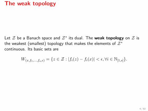
The weak topology
Let Z be a Banach space and Z∗ its dual. The weak topology on Z isthe weakest (smallest) topology that makes the elements of Z∗continuous. Its basic sets are
W(x,f1,...,fs,ε) = z ∈ Z : |fi(z)− fi(x)| < ε,∀i ∈ N[1,s].
4 / 92

The weak topology
A sequence xnn ⊆ Z converges weakly to an element x ∈ Z, denotedby
xnw−→ x,
if for every finite selection of elements of Z∗, f1, . . . , fs it is
|fi(xn)− fi(x)| → 0.
5 / 92

The weak∗ topology
The weak∗ topology on Z∗ is the weakest (smallest) topology whichmakes the maps f 7→ f(x) continuous. Its basic sets are
W ∗(f,x1,...,xs,ε) = g ∈ Z∗ : |g(xi)− f(xi)| < ε,∀i ∈ N[1,s].
6 / 92
The weak∗ topology
Let Z be a Banach space and Z∗ its dual. A sequence fnn ⊆ Z∗converges weakly∗ to an element f ∈ Z∗, denoted by
fnw∗−→ f,
if for every x1, . . . , xs ∈ Z, it is
|fn(xi)− f(xi)| → 0.
This is exactly the notion of pointwise convergence, i.e., fnw∗−→ f
means that the sequence of function fn converges pointwise.
7 / 92
Lp spaces
Let (Ω,F ,P) be a probability space. The space Lp(Ω,F ,P) – p ∈ [1,∞)– is a space of random variables
Z : (Ω,F ,P)→ IR
(F-measurable) equipped with the p-norm:
‖Z‖p =
(∫Ω|Z|pdP
)1/p
= E[|Z|p]1/p
so that the above integral is well-defined and finite.
8 / 92

Lp spaces
If Z ∈ Lp(Ω,F ,P) with p ∈ [1,∞), then the p-th order of Z is finite andall its orders 1 ≤ p′ ≤ p are also finite2, so
Lp(Ω,F ,P) ⊆ Lp′(Ω,F ,P)
2W. Rudin, Real and Complex Analysis, 3rd edition, McGraw-Hill Book Co., NewYork, 1987, Chap. 3, Ex. 7
9 / 92

The space L∞
Let (Ω,F ,P) be a probability space. The space L∞(Ω,F ,P) is a space ofrandom variables
Z : (Ω,F ,P)→ IR
(F-measurable) equipped with the ∞-norm:
‖Z‖∞ = ess supω∈Ω
|Z(ω)|,
so that ‖Z‖∞ is finite.
10 / 92
(In)equality on Lp spaces
Let Z and V be two random variables of Lp(Ω,F ,P). We consider thoseequal if
P(ω ∈ Ω : Z(ω) 6= V (ω)) = 0,
or, what is the sameP(Z 6= V ) = 0,
and we denote Z = V or Z ≡ V 3. Similarly, Z ≤ V means
P(Z > V ) = 0.
The relation ≤ is a partial order on Lp(Ω,F ,P).
3or, sometimes, Z = V a.s. We also define the space Lp(Ω,F ,P) =Lp(Ω,F ,P)/ ≡
11 / 92
Topological dual of Lp spaces
Let X be a Banach space. The topological dual of X, denoted X∗, isthe space of linear continuous (bounded) functional from X to IR. Forx∗ ∈ X∗ we define the scalar product between x∗ and x as
〈x∗, x〉 = x∗(x)
For Lp-spaces with p ∈ (1,∞)we have
(Lp(Ω,F ,P))∗ = Lq(Ω,F ,P),
where q−1 + p−1 = 1 and
(L1(Ω,F ,P))∗ = L∞(Ω,F ,P).
The dual of L∞ is not an Lp-space.
12 / 92

Topological dual of Lp spaces
An element Y ∈ (Lp(Ω,F ,P))∗ is a continuous linear operator
Y : Lp(Ω,F ,P) 3 Z 7→ Y (Z) ∈ IR
where
Y (Z) := 〈Y, Z〉 =
∫ΩY XdP
where Y ∈ Lq(Ω,F ,P). We simply identify Y with Y 4.
4Indeed, such a Y exists; see Theorem 4.4.10 in: D.S. Bridges, Foundations ofreal and abstract analysis, Springer, 1998, p. 202
13 / 92
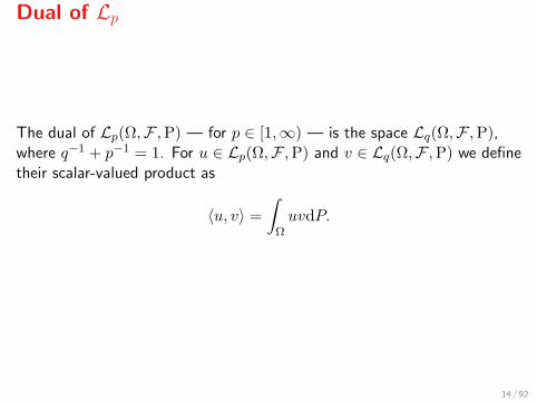
Dual of Lp
The dual of Lp(Ω,F ,P) — for p ∈ [1,∞) — is the space Lq(Ω,F ,P),where q−1 + p−1 = 1. For u ∈ Lp(Ω,F ,P) and v ∈ Lq(Ω,F ,P) we definetheir scalar-valued product as
〈u, v〉 =
∫ΩuvdP.
14 / 92
II. Risk measures
X Risk measures
X Coherent risk measures
X Characterisation of coherency
15 / 92
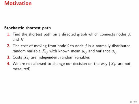
Motivation
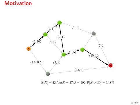
Stochastic shortest path
1. Find the shortest path on a directed graph which connects nodes Aand B
2. The cost of moving from node i to node j is a normally distributedrandom variable Xij with known mean µij and variance σij
3. Costs Xij are independent random variables
4. We are not allowed to change our decision on the way (Xij are notmeasured)
16 / 92

Motivation
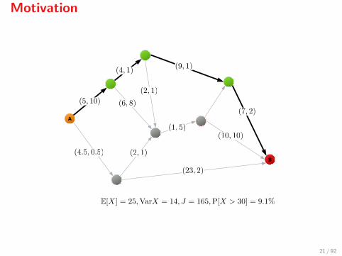
The stochastic shortest path problem amounts to the minimisation of
E[∑i
Xi,i+ ] =∑i
µi,i+ ,
totally disregards any stochastic information (e.g., the variance). Let usdefine
J = E[X] + λVar[X],
where X is the total cost. This is known as the Markowitz risk measure5.
5Markowitz’s mean-variance risk measure was one of the first ways to quantifyrisk in 1952. However, nowadays it doesn’t qualify as a “good” risk measure forreasons we’ll explain in a while.
17 / 92

Motivation
A
B
18 / 92
Motivation
A
B
19 / 92
Motivation
A
B
20 / 92
Motivation
A
B
21 / 92

Motivation
A
B
22 / 92

Motivation
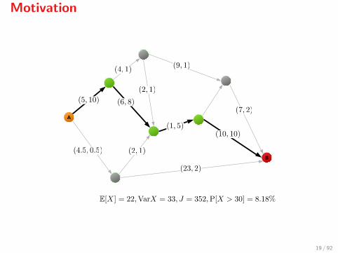
Notice that:
I The stochastic shortest path solution with E[X] = 22 is too riskysince P[X > 30] = 8.18% and Var[X] = 33
I The minimum mean-variance solution with E[X] = 27 is a muchwiser choice since P[X > 30] = 5.69% and Var[X] = 2.5
I The stochastic solution has a mean-risk of J = 352, whereas themean-risk-optimum is at J = 52
Conclusion: E[·] may often be a bad idea...
23 / 92

Risk measures
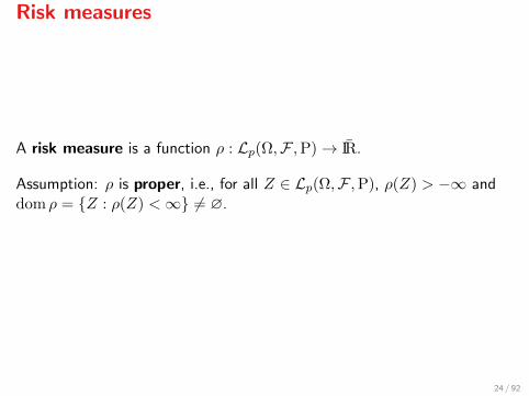
A risk measure is a function ρ : Lp(Ω,F ,P)→ IR.
Assumption: ρ is proper, i.e., for all Z ∈ Lp(Ω,F ,P), ρ(Z) > −∞ anddom ρ = Z : ρ(Z) <∞ 6= ∅.
24 / 92
Risk measures
A risk measure is a function ρ : Lp(Ω,F ,P)→ IR.
Assumption: ρ is proper, i.e., for all Z ∈ Lp(Ω,F ,P), ρ(Z) > −∞ anddom ρ = Z : ρ(Z) <∞ 6= ∅.
24 / 92

Risk measures
Since risk measures are defined on Lp(Ω,F ,P) it is implied that forZ1, Z2 ∈ Lp(Ω,F ,P)
Z1 = Z2 ⇒ ρ(Z1) = ρ(Z2),
and recall that Z1 = Z2 means that
P[Z1 6= Z2] = 0
25 / 92
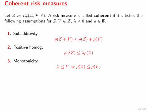
Coherent risk measures
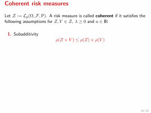
Let Z := Lp(Ω,F ,P). A risk measure is called coherent if it satisfies thefollowing assumptions for Z, V ∈ Z, λ ≥ 0 and a ∈ IR
1. Subadditivityρ(Z + V ) ≤ ρ(Z) + ρ(V )
2. Positive homog.ρ(λZ) ≤ λρ(Z)
3. MonotonicityZ ≤ V ⇒ ρ(Z) ≤ ρ(V )
4. Translation invariance
ρ(Z + a) = a+ ρ(Z)
26 / 92

Coherent risk measures
Let Z := Lp(Ω,F ,P). A risk measure is called coherent if it satisfies thefollowing assumptions for Z, V ∈ Z, λ ≥ 0 and a ∈ IR
1. Subadditivityρ(Z + V ) ≤ ρ(Z) + ρ(V )
2. Positive homog.ρ(λZ) ≤ λρ(Z)
3. MonotonicityZ ≤ V ⇒ ρ(Z) ≤ ρ(V )
4. Translation invariance
ρ(Z + a) = a+ ρ(Z)
26 / 92

Coherent risk measures are convex
Because of the sub-additivity and Positive homogeneity of coherent riskmeasures, they are convex
ρ(λZ + (1− λ)V ) ≤ λρ(Z) + (1− λ)ρ(V ),
for all Z, V ∈ Lp(Ω,F ,P) and λ ∈ [0, 1].
27 / 92

* Bibliographic note
The four coherence conditions are the ones originally stipulated by Artzneret al., 1997.
Shapiro, Dentcheva and Ruszczynski use instead: (i) convexity, (ii)monotonicity, (iii) translation equivariance and (iv) positive homogeneity.These two conventions are of course equivalent.
28 / 92

Convex conjugate mappings
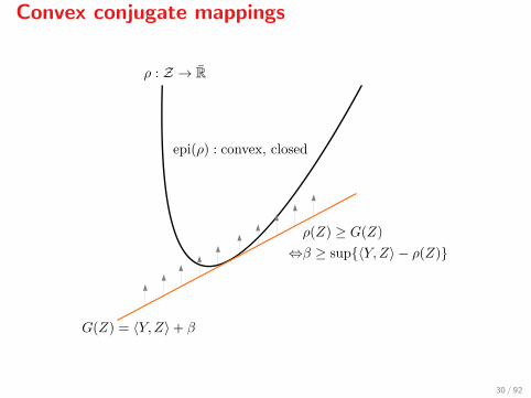
A convex mapping ρ : Z → R can be seen
I As its graph described by Z 7→ ρ(Z)
I As its epigraph, i.e., epi(ρ) = (Z,α) : ρ(Z) ≤ αI And, when the epigraph is closed, it can be written as the intersection
of halfspaces defined by its tangents, i.e., affine functions
G(Z) = 〈Y,Z〉+ β,
with ρ(Z) ≥ G(Z) for all Z.
29 / 92
Convex conjugate mappings
30 / 92
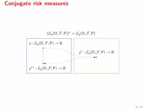
Conjugate risk measures
For a coherent risk measure ρ : Lp(Ω,F ,P)→ IR, the conjugate riskmeasure is a function ρ∗ : Lq(Ω,F ,P)→ IR defined as
ρ∗(Y ) = supZ∈Lp(Ω,F ,P)
〈Z, Y 〉 − ρ(Z),
and the bi-conjudate of ρ is a function ρ∗∗ : Lp(Ω,F ,P)→ IR with
ρ∗∗(Z) = supY ∈Lq(Ω,F ,P)
〈Y, Z〉 − ρ∗(Y ) ,
If ρ is lower semicontinuous, then, by the Fenchel-Moreau theorem,
ρ = ρ∗∗.
31 / 92
Conjugate risk measures
32 / 92
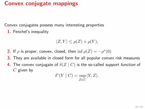
Convex conjugate mappings
Convex conjugates possess many interesting properties
1. Fenchel’s inequality
〈Z, Y 〉 ≤ ρ(Z) + ρ(Y ),
2. If ρ is proper, convex, closed, then inf ρ(Z) = −ρ∗(0)
3. They are available in closed form for all popular convex risk measures
4. The convex conjugate of δ(Z | C) is the so-called support function ofC given by
δ∗(Y | C) = supZ∈C〈Y,Z〉.
33 / 92

The Fenchel-Moreau Theorem
Theorem. Let Z be a Banach space (e.g., any of Lp(Ω,F ,P) withp ∈ [1,∞)) and f : Z → IR be a proper function. Then
f∗∗ = clf.
If, additionally, f is lsc, then
f∗∗ = f.
34 / 92

The Fenchel-Moreau Theorem
Corollary. Assume that ρ : Lp(Ω,F ,P)→ IR is a proper, convex, lowersemi-continuous risk measure. Then,
ρ(Z) = ρ∗∗(Z)
= supY ∈Lq(Ω,F ,P)
〈Y,Z〉 − ρ∗(Y ) ,
= supY ∈dom ρ∗
〈Y, Z〉 − ρ∗(Y ) .
35 / 92

Monotonicity of ρ
The monotonicity property of a proper, convex, lsc risk measure ρ, that is
ρ(Z) ≤ ρ(V ),
whenever Z ≤ V , Z, V ∈ Z, holds iff the elements of the set dom ρ∗ arenonnegative.
36 / 92

Translation equivariance of ρ
The translation equivariance property of a proper, convex, lsc riskmeasure ρ, that is
ρ(Z + c) = ρ(Z) + c,
for all Z ∈ Z, holds iff every ζ ∈ dom ρ∗ satisfies∫ΩζdP = 1.
37 / 92

Positive homogeneity of ρ
A proper, convex, lsc risk measure ρ is positive homogeneous6, that is
ρ(αZ) = αρ(Z),
for all Z ∈ Z and α ≥ 0, iff it is the support function of dom ρ∗, i.e.,
ρ(Z) = supζ∈A〈ζ, Z〉,
where A := dom ρ∗.
6Theorem 13.2 in R.T. Rockafellar, Convex Analysis, Princeton Univ. Press, 1972.
38 / 92

To summarise...
Let ρ : Lp(Ω,F ,P)→ IR, p ∈ [1,∞), be
1. proper, convex, lsc
2. monotone
3. translation invariant
Then,
ρ(Z) = supY ∈A〈Y, Z〉 − ρ∗(Y ) ,
where notice that A is a (w∗-closed) subset of
P =
Y ∈ Lq(Ω,F ,P),
∫ΩY dP = 1, Y ≥ 0
39 / 92

To summarise...
Let ρ : Lp(Ω,F ,P)→ IR, p ∈ [1,∞), be
1. proper, convex, lsc
2. monotone
3. translation invariant
4. positively homogeneous
Then,
ρ(Z) = supY ∈A〈Y, Z〉.
40 / 92

Characterisation of coherent risk measures
Theorem. A risk measure is coherent iff it is the support function of aw∗ closed subset A ⊆ P, that is
ρ(Z) = supY ∈A〈Y,Z〉.
41 / 92

Subdifferentials of risk measures
Let ρ be a convex proper lower semicontinuous risk measure onZ = Lp(Ω,F ,P). Then,
A = ∂ρ(0),
and∂ρ(Z) = arg max
Y ∈A〈Y, Z〉
42 / 92

End of section
In summary:
I Risk measures extract a characteristic value ρ[Z] out of a randomvariable Z ∈ Lp(Ω,F ,P)
I Risk measures are sufficiently regular if they satisfy four coherenceaxioms: convexity, monotonicity, translation equivariance and positivehomogeneity
I Using the Fenchel-Moreau Theorem coherent risk measures can bewritten as the supremum of the expectation of Z, Eµ[Z] over a set ofa set of distributions µ ∈ A
I Sub-differentiability and continuity properties of coherent riskmeasures are rather well understood
43 / 92

III. Examples of risk measures
X Incoherent risk measures
? Mean-variance? Value-at-risk
X Coherent risk measures
? Mean-upper-semideviation of order p? Average value-at-risk
44 / 92

Mean-variance
A simple (non coherent) risk measure is the mean-variance defined as
ρ(Z) = E[Z] + cVar[Z].
45 / 92
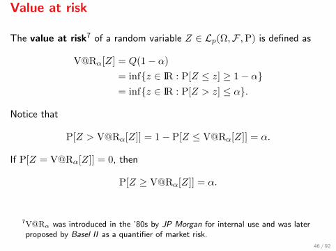
Value at risk
The value at risk7 of a random variable Z ∈ Lp(Ω,F ,P) is defined as
V@Rα[Z] = Q(1− α)
= infz ∈ IR : P[Z ≤ z] ≥ 1− α= infz ∈ IR : P[Z > z] ≤ α.
Notice that
P[Z > V@Rα[Z]] = 1− P[Z ≤ V@Rα[Z]] = α.
If P[Z = V@Rα[Z]] = 0, then
P[Z ≥ V@Rα[Z]] = α.
7V@Rα was introduced in the ’80s by JP Morgan for internal use and was laterproposed by Basel II as a quantifier of market risk.
46 / 92
Value at risk
The value-at-risk is not a coherent risk measure, although it satisfies
V@Rα[Z + c] = V@Rα[Z] + c,
because it is not subadditive (although it turns out to be subadditive fornormally distributed RVs).
47 / 92
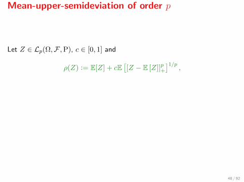
Mean-upper-semideviation of order p
Let Z ∈ Lp(Ω,F ,P), c ∈ [0, 1] and
ρ(Z) := E[Z] + cE[[Z − E [Z]]p+
]1/p,
This is clearly subadditive, translation equivariant, pos. homogeneous and
A =
Y ∈ Lq(Ω,F ,P)
∣∣∣∣ Y = 1 +G− E[G],‖G‖q ≤ c,G ≥ 0
.
All elements of A are positive, thus ρ is monotonous.
48 / 92
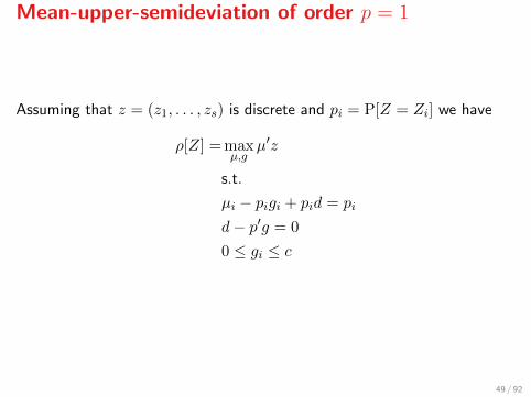
Mean-upper-semideviation of order p = 1
Assuming that z = (z1, . . . , zs) is discrete and pi = P[Z = Zi] we have
ρ[Z] = maxµ,g
µ′z
s.t.
µi − pigi + pid = pi
d− p′g = 0
0 ≤ gi ≤ c
49 / 92

Computation of MUS of order p = 1
function M = mus(Z, p, c)
% Computation using the definition% Z Discrete values of random variable Z% p Probability values% c Parameter c of MUS% M Mean−upper semideviation with parameter c
EZ = sum(p.*Z);
M = EZ + c* sum(p.*max(Z-EZ, zeros(size(Z))));
50 / 92
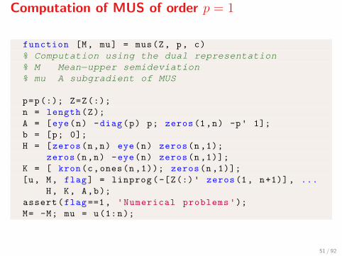
Computation of MUS of order p = 1
function [M, mu] = mus(Z, p, c)
% Computation using the dual representation% M Mean−upper semideviation% mu A subgradient of MUS
p=p(:); Z=Z(:);
n = length(Z);
A = [eye(n) -diag(p) p; zeros(1,n) -p' 1];
b = [p; 0];
H = [zeros(n,n) eye(n) zeros(n,1);
zeros(n,n) -eye(n) zeros(n,1)];
K = [ kron(c,ones(n,1)); zeros(n,1)];
[u, M, flag] = linprog(-[Z(:)' zeros(1, n+1)], ...
H, K, A,b);
assert(flag==1, 'Numerical problems ');M= -M; mu = u(1:n);
51 / 92

Average value-at-risk
The average value-at-risk8 of a Z ∈ Z = L1(Ω,F ,P) is
AV@Rα(Z) := inft∈IRt+ α−1E[Z − t]+,
where is the inf attained?
8aka expected shortfall and expected tail loss.
52 / 92

Average value-at-risk
For given Z ∈ Z define
φ(t) := t+ α−1E[Z − t]+
If HZ is continuous at t, then φ is differentiable at t and9
φ′(t) = 1 + α−1(HZ(t)− 1).
The minimum of φ is attained where φ′(t∗) = 0, i.e., over the interval[t∗, t∗∗] where
t∗ = inft : HZ(t) ≥ 1− αt∗∗ = supt : HZ(t) ≤ 1− α
9Exercise: Prove that when E[Z − t]+ is diff/ble at t, then ddtE[Z − t]+ =
HZ(t)− 1. Use the fact that E[Z − t]+ = E[(Z − t)1[Z≥t]].
53 / 92

Average value-at-risk
The infimum is attained for t ∈ [t∗, t∗∗] where
t∗ = inft : HZ(t) ≥ 1− α = V@Rα(Z),
that isAV@Rα(Z) = t∗ + α−1E[Z − t∗]+.
54 / 92

Average value-at-risk
An alternative representation:
AV@Rα[Z] = t∗ + α−1E[Z − t∗]+
= t∗ + α−1
∫ +∞
−∞[Z − t∗]+dP
= t∗ + α−1
∫ +∞
t∗(Z − t∗)dP
= t∗ + α−1
∫ +∞
t∗ZdP− t∗α−1
∫ +∞
t∗dP︸ ︷︷ ︸
P[Z≥t∗]=α
= α−1
∫ +∞
t∗ZdP.
55 / 92
Average value-at-risk
Assuming P[Z = V@Rα[Z]] = 0 we have
P[Z ≥ V@Rα[Z]] = α
we have another representation of AV@Rα
AV@Rα[Z] = α−1
∫ +∞
V@Rα[Z]ZdP.
= E [Z | Z ≥ V@Rα [Z]] .
This is because for E ∈ F ,
E[Z | E] =E[1EZ]
P[E]
56 / 92

Average value-at-risk
`
`
57 / 92
Average value-at-risk
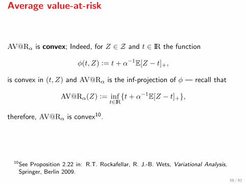
AV@Rα is convex; Indeed, for Z ∈ Z and t ∈ IR the function
φ(t, Z) := t+ α−1E[Z − t]+,
is convex in (t, Z) and AV@Rα is the inf-projection of φ — recall that
AV@Rα(Z) := inft∈IRt+ α−1E[Z − t]+,
therefore, AV@Rα is convex10.
10See Proposition 2.22 in: R.T. Rockafellar, R. J.-B. Wets, Variational Analysis,Springer, Berlin 2009.
58 / 92
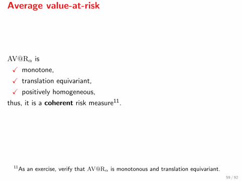
Average value-at-risk
AV@Rα is
X monotone,
X translation equivariant,
X positively homogeneous,
thus, it is a coherent risk measure11.
11As an exercise, verify that AV@Rα is monotonous and translation equivariant.
59 / 92

Average value-at-risk
The conjugate function of AV@Rα is
(AV@Rα)∗[Y ] = supZ∈Z〈Y,Z〉 −AV@Rα[Z]
= supZ∈Z〈Y,Z〉 − inf
tt+ α−1E[Z − t]+
= supZ,t〈Y, Z〉 − t− α−1E[Z − t]+
= supS,t〈Y, S〉 − 〈Y − 1, t〉 − α−1E[S]+,
whose domain is12
A = Y ∈ Z∗ : E[Y ] = 1, Y (ω) ∈ [0, α−1], for a.e. ω ∈ Ω.
12Exercise: Verify that this is indeed the domain of (AV@Rα)∗.
60 / 92

Average value-at-risk
AV@Rα[Z] can be written as
AV@Rα[Z] = supY ∈Z
〈Y,Z〉 : E[Y ] = 1, Y ∈ [0, α−1], a.e.
In case Ω = ω1, . . . , ωK and pi := P[ω = ωi] then AV@Rα is computedvia the following LP
AV@Rα[Z] = maxY ∈IRK
∑piYiZi︸ ︷︷ ︸〈Y,Z〉
s.t.∑
piYi = 1
0 ≤ Yi ≤ α−1
61 / 92
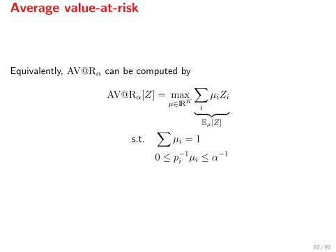
Average value-at-risk
Equivalently, AV@Rα can be computed by
AV@Rα[Z] = maxµ∈IRK
∑i
µiZi︸ ︷︷ ︸Eµ[Z]
s.t.∑
µi = 1
0 ≤ p−1i µi ≤ α−1
62 / 92
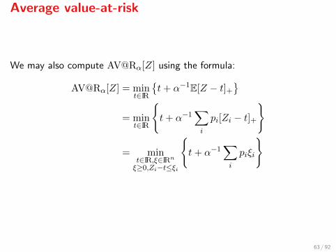
Average value-at-risk
We may also compute AV@Rα[Z] using the formula:
AV@Rα[Z] = mint∈IR
t+ α−1E[Z − t]+
= min
t∈IR
t+ α−1
∑i
pi[Zi − t]+
= mint∈IR,ξ∈IRn
ξ≥0,Zi−t≤ξi
t+ α−1
∑i
piξi
63 / 92

Subdifferential of AV@Rα[·]
AV@Rα is subdifferentiable with
∂(AV@Rα)[Z] = arg maxY ∈A
〈Y, Z〉
= arg maxY ∈Z∗
〈Y,Z〉 : Y ∈ [0, α−1], a.e. ,E[Y ] = 1
.
Relaxing the equality constraint E[Y ] = 1 we have the Lagrangian
L(Y, λ;Z) = 〈Y,Z〉+ λ(1− E[Y ])
= 〈Y,Z〉+ λ− 〈λ, Y 〉= 〈Y,Z − λ〉+ λ.
64 / 92

Subdifferential of AV@Rα[·]
We can now introduce the dual function
q(λ) = supY ∈[0,α−1]
L(Y, λ)
= supY ∈[0,α−1]
〈Y, Z − λ〉+ λ
= supY ∈[0,α−1]
∫Y (Z − λ)dP + λ,
the supremum is attained for Y = α−11[Z−λ≥0], so
q(λ) = α−1E[Z − λ]+ + λ.
65 / 92
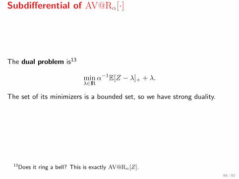
Subdifferential of AV@Rα[·]
The dual problem is13
minλ∈IR
α−1E[Z − λ]+ + λ.
The set of its minimizers is a bounded set, so we have strong duality.
13Does it ring a bell? This is exactly AV@Rα[Z].
66 / 92

Subdifferential of AV@Rα[·]
We may now compute the subdifferential of AV@Rα[Z]. Assume t∗ = t∗∗.Then a Y ∈ ∂(AV@Rα)[Z] must satisfy
E[Y ] = 1
Z > t∗ ⇒ Y = α−1
Z < t∗ ⇒ Y = 0
Z = t∗ ⇒ Y ∈ [0, α−1]
67 / 92
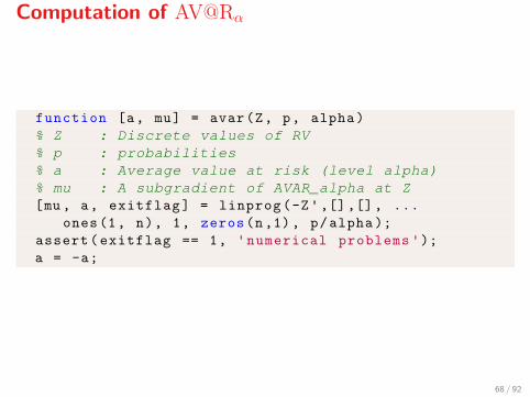
Computation of AV@Rα
function [a, mu] = avar(Z, p, alpha)
% Z : Discrete values of RV% p : probabilities% a : Average value at risk (level alpha)% mu : A subgradient of AVAR_alpha at Z[mu, a, exitflag] = linprog(-Z',[],[], ...
ones(1, n), 1, zeros(n,1), p/alpha);
assert(exitflag == 1, 'numerical problems ');a = -a;
68 / 92
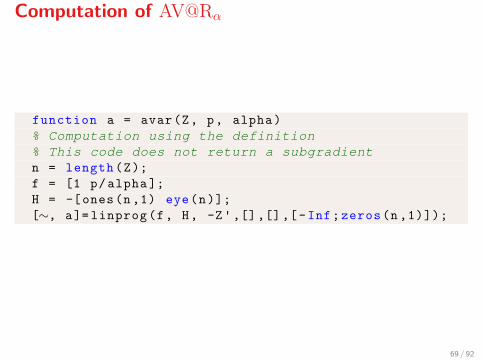
Computation of AV@Rα
function a = avar(Z, p, alpha)
% Computation using the definition% This code does not return a subgradientn = length(Z);
f = [1 p/alpha ];
H = -[ones(n,1) eye(n)];
[∼, a]= linprog(f, H, -Z',[],[],[-Inf;zeros(n ,1)]);
69 / 92
* Remark
Take Z ≥ 0. AV@Rα[Z] can be defined as follows14
AV@R1[Z] = E[Z | Z ≥ V@R1[Z]]
= E[Z | Z ≥ ess sup[Z]
= ess sup[Z],
and AVAR0[Z] isAVAR0[Z] = E[Z]
AV@Rα can be used to bridge the distance between the robust (‖ · ‖∞)and the stochastic (E[·]) approach.
14Note that V@R1[Z] = −∞ and V@R0[Z] = ess sup[Z]
70 / 92

IV. Law invariance
X Equality of distributions
X Law invaraince
X Kusuoka’s Representation Theorem
X Stochastic orders
71 / 92

Equality of distributions
Let Ω = ω1, ω2, ω3, F = 2Ω and P[ω = ωi] = 1/3. Let X be a randomvariable with
X(ω) = ω
for all ω ∈ Ω. Define a random variable Y with
Y (ω1) = ω2,
Y (ω2) = ω3,
Y (ω3) = ω1,
Then, X and Y have the same distribution, but they are never equal:
P[X = ωi] = P[Y = ωi] = 1/3.
72 / 92

Equality of distributions
Let (Ω,F ,P) be a probability space and X : Ω→ IR a N (0, 1)-distributedrandom variable.
Define the random variableY = −X.
Then, Y ∼ N (0, 1) but X and Y are a.e. unequal:
P[X = Y ] = 0.
73 / 92

Equality of distributions
Two random variables X,Y : Ω→ IR are surely equal if
X(ω) = Y (ω), for all ω ∈ Ω.
They are almost surely equal if
P[X 6= Y ] = P[ω : X(ω) 6= Y (ω)] = 0
They are equal in distribution, denoted as Xd∼ Y , if
P[X ≤ c] = P[Y ≤ c], for all c ∈ IR.
74 / 92

Equality of distributions
A distribution is like a musical score, whereas a random variable is aparticular performance.
75 / 92

Equality of distributions
It is obvious thatX = Y ⇒ X
a.e.= Y ⇒ X
d∼ Y.
76 / 92

Law invariance
A risk measure ρ is called law invariant if, i.e.,
Xd∼ Y ⇒ ρ(X) = ρ(Y ).
i.e., it is insensitive to how the uncertainty is produced (i.e., X(ω)) anddepends only on the distribution.
77 / 92

Law invariance importance
I Law invariance is a natural assumption for risk measures
I It is very often a necessary assumption
I Necessary assumption when studying stochastic orders
I Law invariant, coherent, lsc risk measures can be constructed usingcombinations of the average value-at-risk (Kusuoka theorem)
78 / 92
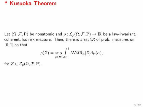
* Kusuoka Theorem
Let (Ω,F ,P) be nonatomic and ρ : Lp(Ω,F ,P)→ IR be a law-invariant,coherent, lsc risk measure. Then, there is a set M of prob. measures on(0, 1] so that
ρ(Z) = supµ∈M
∫ 1
0AV@Rα[Z]dµ(α),
for Z ∈ Lp(Ω,F ,P).
79 / 92

Stochastic orders
For random variables on Lp(Ω,F ,P), we may define various partial orders,known as stochastic orders:
I Integral stochastic orders
I Usual stochastic order
I First, second and k-th stochastic orders
I Increasing convex order
I and many many another...
Hereafter, we shall assume that (Ω,F ,P) is nonatomic.
80 / 92

Stochastic orders
The stochastic orders we will present here are partial orders, i.e.,
1. reflexive (X X)
2. transitive (X Y and Y Z implies X Z)
3. antisymmetric (X Y and Y X implies Yd∼ X)
but not complete, i.e., there will be X,Y such that neither X Y norY X.
81 / 92

Integral stochastic order
Let U be a collection of F-measurable functions u : IR→ IR. This definesa partial order U known as integral stochastic order with generator Uand is defined as
Z1 U Z2 ⇔ E[u(Z1)] ≤ E[u(Z2)],
for all u ∈ U .
82 / 92
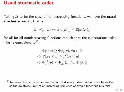
Usual stochastic order
Taking U to be the class of nondecreasing functions, we have the usualstochastic order, that is
Z1 (1) Z2 ⇔ E[u(Z1)] ≤ E[u(Z2)],
for all for all nondecreasing functions u such that the expectations exist.This is equivalent to15
ΦZ1(η) ≥ ΦZ2(η), ∀η ∈ IR
⇔ P[Z1 ≤ η] ≥ P[Z2 ≤ η]
⇔ Φ−1Z1
(p) ≤ Φ−1Z2
(p), ∀p ∈ [0, 1]
15To prove this fact you can use the fact that measurable functions can be writtenas the pointwise limit of an increasing sequence of simple functions (exercise).
83 / 92

Usual stochastic order
Let Z1, Z2 : Lp(Ω,F ,P)→ IR. Then,
Z1 (1) Z2
iff there is a probability space (Ω′,F ′,P′) and random variables Z ′1d∼ Z1,
Z ′2d∼ Z2 so that
Z ′1 ≤ Z ′2 P′ -a.e.
These are
Z ′i = Φ−1Zi
(U),
where U is the uniform RV on Lp(Ω,F ,P).
84 / 92

Usual stochastic order
Let Z1, Z2 : Lp(Ω,F ,P)→ IR. Then,
Z1 (1) Z2
iff there is a probability space (Ω′,F ′,P′) and random variables Z ′1d∼ Z1,
Z ′2d∼ Z2 so that
Z ′1 ≤ Z ′2 P′ -a.e.
These are
Z ′i = Φ−1Zi
(U),
where U is the uniform RV on Lp(Ω,F ,P).
84 / 92
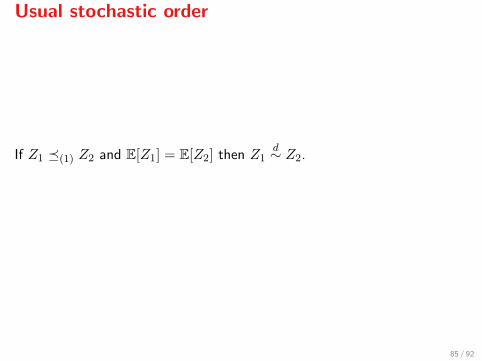
Usual stochastic order
If Z1 (1) Z2 and E[Z1] = E[Z2] then Z1d∼ Z2.
85 / 92
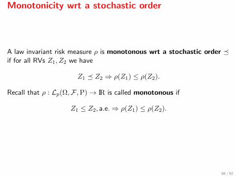
Monotonicity wrt a stochastic order
A law invariant risk measure ρ is monotonous wrt a stochastic order if for all RVs Z1, Z2 we have
Z1 Z2 ⇒ ρ(Z1) ≤ ρ(Z2).
Recall that ρ : Lp(Ω,F ,P)→ IR is called monotonous if
Z1 ≤ Z2, a.e.⇒ ρ(Z1) ≤ ρ(Z2).
86 / 92
Monotonicity wrt (1)
Assume (Ω,F ,P) is nonatomic. Let ρ be law invariant. TFAE:
1. ρ is monotonous
2. ρ is monotonous wrt (1)
Proof. (1⇒2) Take Z1 (1) Z2, and define the RVs Zi , Φ−1Zi
(U) on
(Ω′,F ′,P′) so that Z ′id∼ Zi. We have Z ′1 ≤ Z ′2 P′-a.e. on Ω′. Since ρ is
monotonous it is ρ(Z ′1) ≤ ρ(Z ′2) and monotonicity wrt (1) followsbecause ρ is law invariant. The converse is straightforward (exercise).
87 / 92

Increasing convex order
Taking U to be the class of nondecreasing convex functions, we have theincresing convex order, that is
Z1 icx Z2 ⇔ E[u(Z1)] ≤ E[u(Z2)],
for all nondecreasing convex functions u such that the expectations exist.
88 / 92

Increasing convex order
For two random variables Z1, Z2 ∈ Lp(Ω,F ,P), TFAE:
1. Z1 icx Z2,
2. E[Z1 − η]+ ≤ E[Z2 − η]+, for all η ∈ IR.
89 / 92
Monotonicity wrt icx
Assume (Ω,F ,P) is nonatomic. Any law invariant, lsc and coherent riskmeasure ρ : Lp(Ω,F ,P)→ IR is monotonous wrt icx.
Proof. (1⇒2) It is easy to show that AV@Rα is monotonous wrt icx.The proof follows invoking the Kusuoka representation theorem.
90 / 92
Additional info cannot increase risk
Let (Ω,F ,P) be nonatomic, G ⊆ F be a sub-σ-algebra of F andρ : Lp(Ω,F ,P)→ IR be law invariant, lsc and coherent. Then,
ρ(E[Z | G]) ≤ ρ(Z),
for all Z ∈ Lp(Ω,F ,P). Additionally,
E[Z] ≤ ρ(Z).
91 / 92
Further reading
1. A. Shapiro, D. Dentcheva, and A.P. Ruszczynski, Lectures on stochasticprogramming: modeling and theory, SIAM 2009.
2. H. Follmer and A. Schied, Stochastic Finance - an introduction in discrete time,Walter de Gruyter, Berlin, 2004.
3. N. Bauerle and A. Muller, Stochastic Orders and Risk Measures: Consistency andBounds, Insurance: Mathematics and Economics 38(1), pp.132–138, 2005.
4. A. Shapiro, On Kusuoka representation of law invariant risk measures,Mathematics of Operations Research 38(1), pp. 142-152, 2013.
5. Lecture notes of course EE365 Standford University available athttp://stanford.edu/class/ee365/lectures.html
6. P. Artzner, F. Delbaen, J.M. Eber, and D. Heath. Thinking coherently, Risk10(11):68–71, 1997.
7. S. Mitra, Risk Measures in Quantitative Finance, arXiv:0904.0870, 2009.
92 / 92