Risk Management & Real Options VII. The Value of Information Stefan Scholtes Judge Institute of Management University of Cambridge MPhil Course 2004-05

Risk Management & Real Options

VII. The Value of Information

Stefan ScholtesJudge Institute of Management

University of Cambridge

MPhil Course 2004-05

2 September 2004 © Scholtes 2004 Page 2

Course content

I. IntroductionII. The forecast is always wrong

I. The industry valuation standard: Net Present Value

II. Sensitivity analysisIII. The system value is a shape

I. Value profiles and value-at-risk charts

II. SKILL: Using a shape calculatorIII. CASE: Overbooking at EasyBeds

IV. Developing valuation modelsI. Easybeds revisited

V. Designing a system means sculpting its value shapeI. CASE: Designing a Parking Garage

III. The flaw of averages: Effects of

system constraintsVI. Coping with uncertainty I:

DiversificationI. The central limit theoremII. The effect of statistical

dependenceIII. Optimising a portfolio

VII. Coping with uncertainty II: The value of information

I. SKILL: Decision Tree Analysis

II. CASE: Market Research at E-Phone

2 September 2004 © Scholtes 2004

Decision Trees

Graphical tool for analysing decisions under risk• Helps to structure the decisions to be made• Shows the dependency of the decisions on uncertain events

Useful when • a sequence of decisions has to be made• the result of each decision is influenced by uncertain events• we have some information about the probability of each event

Cash flowCash flow

Cash flowCash flow

Cash flowCash flow

ProbabilityProbability

ProbabilityProbability

Cash flowCash flow

Cash flowCash flow

TimeTime


0 0

Bid?

30.0%

$20,000 15000

Competing Bid?

0

80.0%

$20,000 15000

70.0% Win bid?

0

20.0%

0 -5000

How much?

-$5,000

30.0%

$25,000 20000

Competing Bid?

0

40.0%

$25,000 20000

70.0% Win bid?

0

60.0%

0 -5000

30.0%

$30,000 25000

Competing Bid?

0

10.0%

$30,000 25000

70.0% Win bid?

0

90.0%

0 -5000

SciTools Bidding

No

Yes

$115K

$120K

$125K

No

Yes

No

Yes

No

Yes

Yes

No

Yes

No

Yes

No

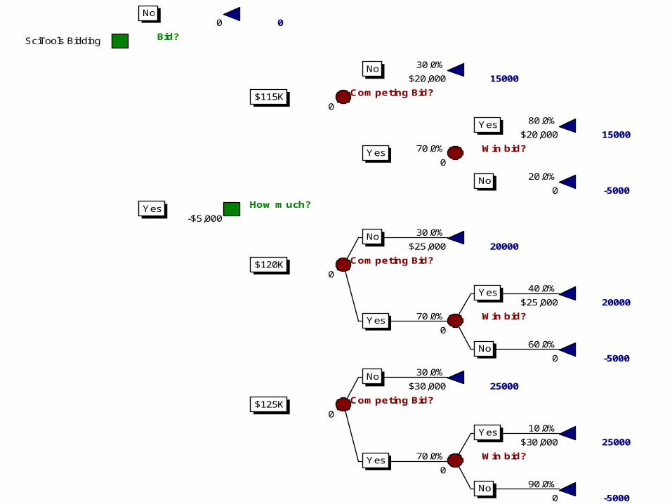
A small but realistic exampleA small but realistic example


Product development (pharmaceutical industry) Marketing (introducing a new product) Oil exploration Bidding for contracts Medical diagnosis ETC.

Prevalent application areas


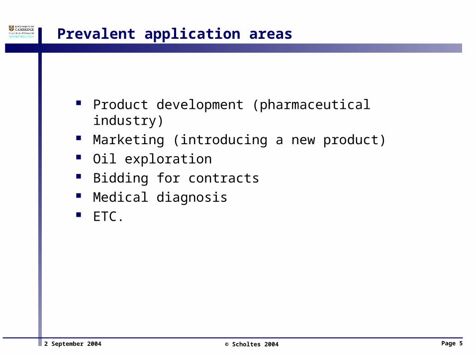
SciTools Case (W/A)

SciTools Inc. specialises in scientific instruments Invited to bid for government contract

• Deliver a specific number of instruments• Sealed bid auction, lowest bid wins

$5,000 to prepare bid Cost of instruments to be delivered: $95,000 SciTools estimates a 30% chance of no competing bid If there is a competing bid, past contract data suggests the

following ranges and probabilities

Lowest competing bid Probability

below $115,000 20%

$115,000 - $120,000 40%

$120,000 - $125,000 30%

above $125,000 10%


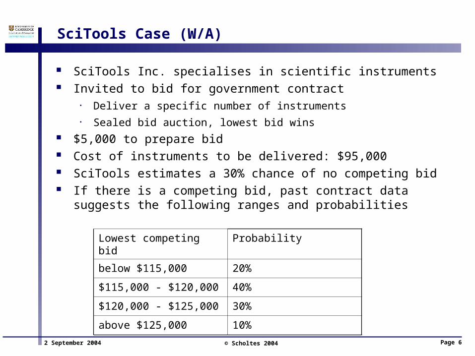
Payoff table

Lists payoff for each possible scenario and each possible decision

Lowest competing bid

no bid below 115,000

115,000 –120,000

120,000 – 125,000

above 125,000

SciToolBid

No bid 0 0 0 0 0

115,000 15,000 - 5,000 15,000 15,000 15,000

120,000 20,000 - 5,000 - 5,000 20,000 20,000

125,000 25,000 - 5,000 - 5,000 - 5,000 25,000

Probability

30% 14% 28% 21% 7%


Time line of decisions and events

Bid? How much? Competing bid? Win bid? Payoff

ActionsActions(under our control)(under our control)

EventsEvents(not under our control)(not under our control)

ResultResult(function of actions(function of actions

and events)and events)


Bid?

Competing Bid?

Win bid?

How much?

Competing Bid?

Win bid?

Competing Bid?

Win bid?

SciTools Bidding

No

Yes

$115K

$120K

$125K

No

Yes

No

Yes

No

Yes

Yes

No

Yes

No

Yes

No


0

Bid?

30.0%

$20,000

Competing Bid?

0

80.0%

$20,000

70.0% Win bid?

0

20.0%

0

How much?

-$5,000

30.0%

$25,000

Competing Bid?

0

40.0%

$25,000

70.0% Win bid?

0

60.0%

0

30.0%

$30,000

Competing Bid?

0

10.0%

$30,000

70.0% Win bid?

0

90.0%

0

SciTools Bidding

No

Yes

$115K

$120K

$125K

No

Yes

No

Yes

No

Yes

Yes

No

Yes

No

Yes

No

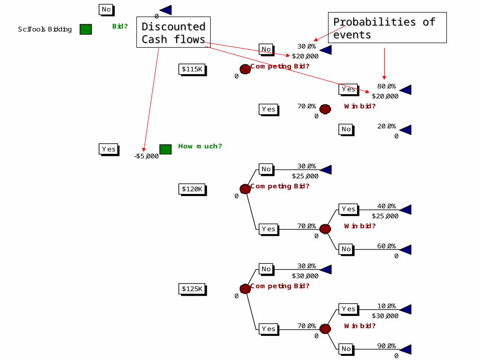
DiscountedDiscountedCash flowsCash flows

Probabilities of Probabilities of eventsevents


0 0

Bid?

30.0%

$20,000 15000

Competing Bid?

0

80.0%

$20,000 15000

70.0% Win bid?

0

20.0%

0 -5000

How much?

-$5,000

30.0%

$25,000 20000

Competing Bid?

0

40.0%

$25,000 20000

70.0% Win bid?

0

60.0%

0 -5000

30.0%

$30,000 25000

Competing Bid?

0

10.0%

$30,000 25000

70.0% Win bid?

0

90.0%

0 -5000

SciTools Bidding

No

Yes

$115K

$120K

$125K

No

Yes

No

Yes

No

Yes

Yes

No

Yes

No

Yes

No

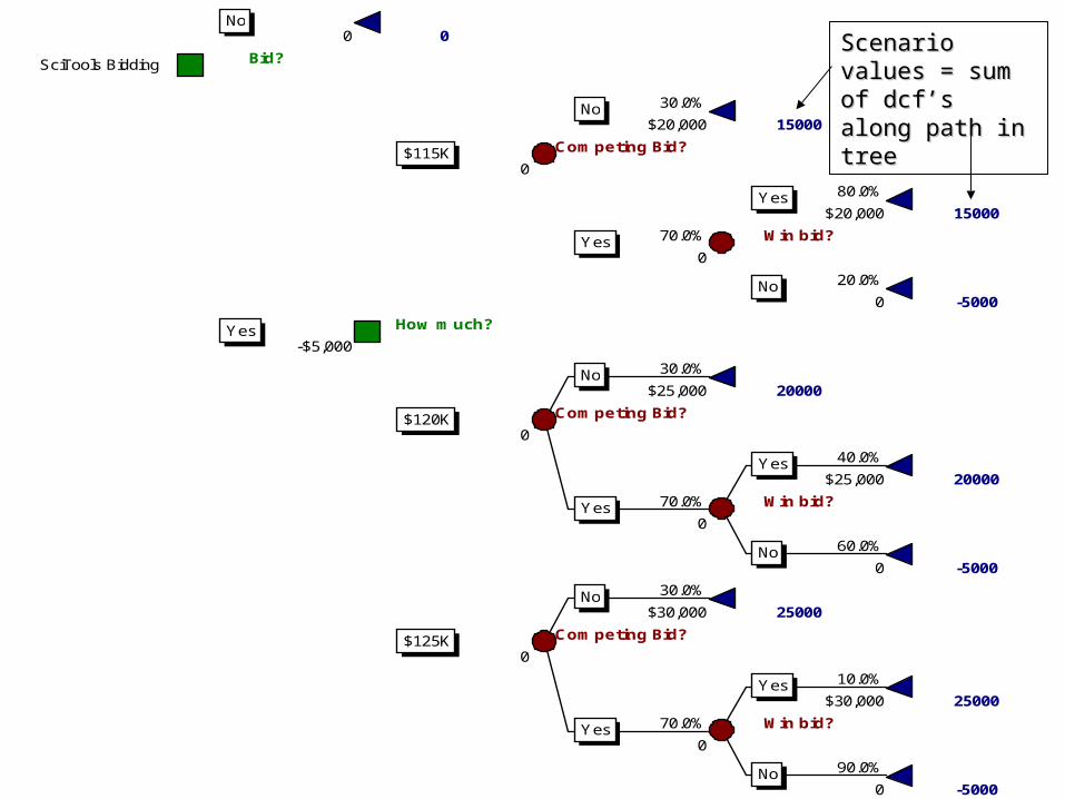
Scenario values = Scenario values = sum of dcf’s sum of dcf’s along path in treealong path in tree


Valuing a tree

Each path through the tree has a value - but which path will the project take?

• Control at decision nodes• Chance at chance nodes

Want to optimise decision: Choose the decision that maximises the value of the project

• Value at decision point depends on the future• But value at a point in the future does not depend on how I reached

this point• Sunk cost argument – think forward, not backwards

Key idea: When valuing the nodes, start in the future, not in the past!

• We know the value of the project at all possible final states• Go backwards in time, valuing nodes successively


Valuing decision nodes

£ 3,000£ 3,000

£ 1,200£ 1,200

Which action would you choose?Which action would you choose?

ExpandExpand

Don’t expandDon’t expand


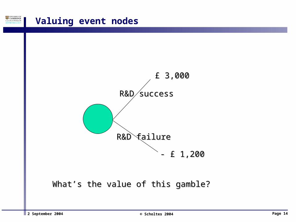
Valuing event nodes

£ 3,000£ 3,000

- £ 1,200- £ 1,200

What’s the value of this gamble? What’s the value of this gamble?

R&D successR&D success

R&D failureR&D failure


Valuing event nodes

£ 3,000£ 3,000

- £ 1,200- £ 1,200

Expected value = 0.4* £ 3,000-0.6* £ 1,200 = £480Expected value = 0.4* £ 3,000-0.6* £ 1,200 = £480



40%40%

60%60%


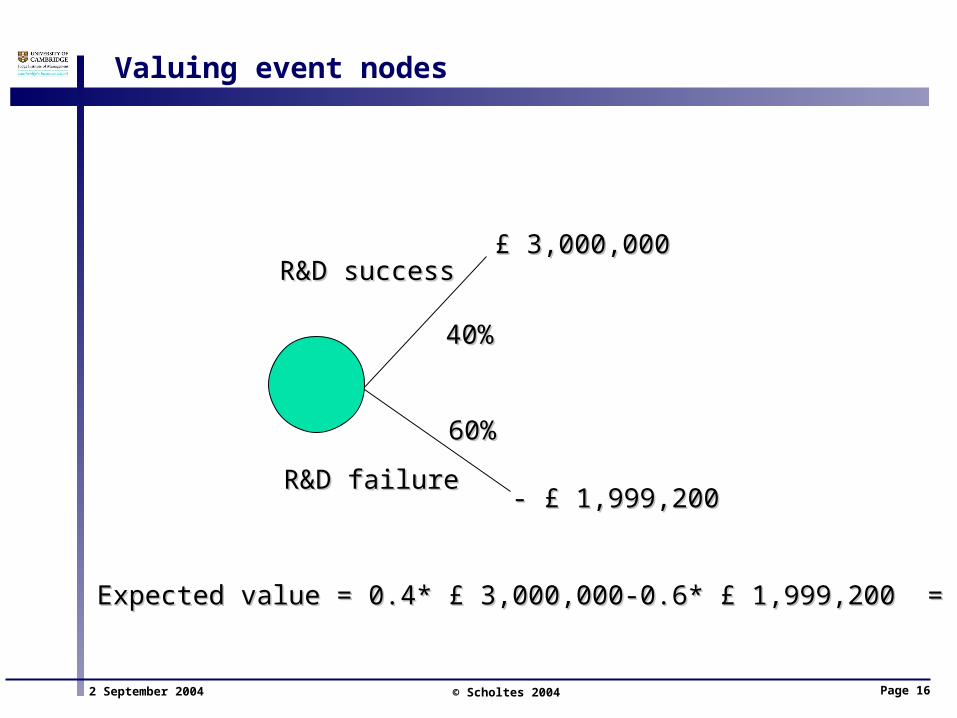
Valuing event nodes

£ 3,000,000£ 3,000,000

- £ 1,999,200- £ 1,999,200

Expected value = 0.4* £ 3,000,000-0.6* £ 1,999,200 = £480Expected value = 0.4* £ 3,000,000-0.6* £ 1,999,200 = £480



40%40%

60%60%


Risk aversion

KEY PROBLEM: If you want to “optimise” your actions you must put a “price-tag” on the chance nodes

• How else would you know how to choose the “best” action?

People are risk-averse and want to be rewarded for risk taking• Simple solution: use risk-premium to discount expected values

Value = Expected Value / (1 + Risk Premium)• But: What’s the “correct” risk premium?

The subject of decision analysis, as an academic discipline, is largely concerned with “how to put a price tag on a chance node”

• Utility theory, real options, etc.

For the sake of this course we assume that decision makers work with expectations, possibly adjusted by risk-premium discounting


0 0

Bid?

30.0%

$20,000 15000

Competing Bid?

0

80.0%

$20,000 15000

70.0% Win bid?

0

20.0%

0 -5000

How much?

-$5,000

30.0%

$25,000 20000

Competing Bid?

0

40.0%

$25,000 20000

70.0% Win bid?

0

60.0%

0 -5000

30.0%

$30,000 25000

Competing Bid?

0

10.0%

$30,000 25000

70.0% Win bid?

0

90.0%

0 -5000

SciTools Bidding

No

Yes

$115K

$120K

$125K

No

Yes

No

Yes

No

Yes

Yes

No

Yes

No

Yes

No


FALSE 0

0 0

Bid?

12200

30.0% 0.3

$20,000 15000

TRUE Competing Bid?

0 12200

80.0% 0.56

$20,000 15000

70.0% Win bid?

0 11000

20.0% 0.14

0 -5000

TRUE How much?

-$5,000 12200

30.0% 0

$25,000 20000

FALSE Competing Bid?

0 9500

40.0% 0

$25,000 20000

70.0% Win bid?

0 5000

60.0% 0

0 -5000

30.0% 0

$30,000 25000

FALSE Competing Bid?

0 6100

10.0% 0

$30,000 25000

70.0% Win bid?

0 -2000

90.0% 0

0 -5000

SciTools Bidding

No

Yes

$115K

$120K

$125K

No

Yes

No

Yes

No

Yes

Yes

No

Yes

No

Yes

No

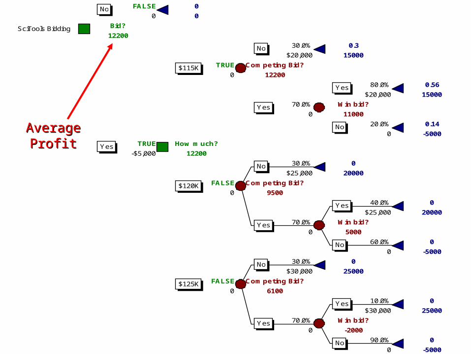
AverageAverageProfitProfit


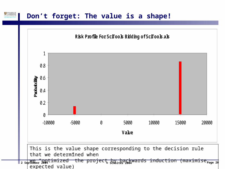
Risk Profile For SciTools Bidding of SciTools.xls

0

0.2

0.4

0.6

0.8

1

-10000 -5000 0 5000 10000 15000 20000

Value

Prob

abili

ty

Don’t forget: The value is a shape!

This is the value shape corresponding to the decision rule that we determined when we “optimized” the project by backwards induction (maximise expected value)


Sensitivity analysis

Managerial analyses are based on projections and subjective judgement

• Even if past data is used extensively, why should the future be similar to the past?

“Shake the ladder before you climb it”: Test how robust your conclusions are w.r.t. your input assumptions

• Probabilities on branches• Costs• Demand• Market prices• Etc.


Expected Profit vs. Bid Costs

11600

11800

12000

12200

12400

12600

12800

4400 4600 4800 5000 5200 5400 5600

Bid Costs

Pro

fit

E


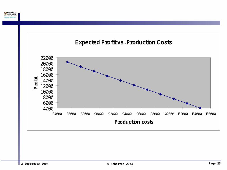
Expected Profit vs. Production Costs

400060008000

10000120001400016000180002000022000

84000 86000 88000 90000 92000 94000 96000 98000 100000 102000 104000 106000

Production costs

Pro

fit


Expected Profit vs. Probability of competing bid

120001205012100121501220012250123001235012400

0.24 0.26 0.28 0.3 0.32 0.34 0.36

Probability of competing bid

Pro

fit


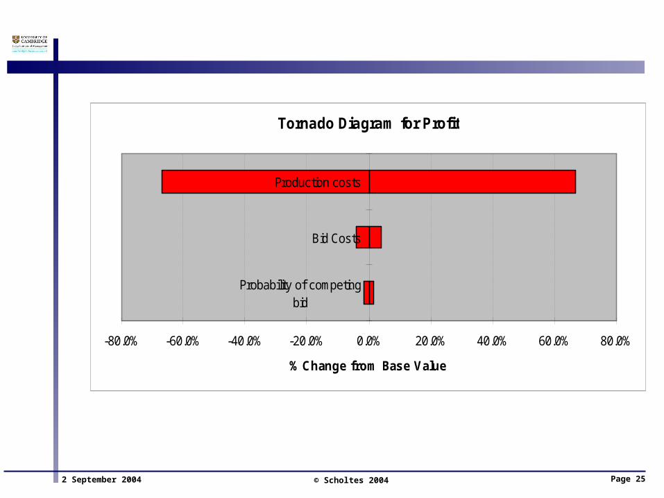
Tornado Diagram for Profit

-80.0% -60.0% -40.0% -20.0% 0.0% 20.0% 40.0% 60.0% 80.0%

Probability of competingbid

Bid Costs

Production costs

% Change from Base Value


Group-work: E-Phone case


ePhone product launch

Fixed cost of 5 Mio units production facility = $60 Mio Unit margin = $20 Mio Cost of test market = $ 5 Mio Demand scenarios

Test effectiveness

Success Survival Failure

Global 5 Mio 2 Mio 0.8 Mio

Test market 150,00 60,000 24,000

Probability of test market outcome

40% 50% 10%

Test Global -> Success Survival Failure

Success 60% 30% 10%

Survival 15% 70% 15%

Failure 10% 30% 60%


Value of (imperfect) information

Test provides information by changing probabilities of market scenarios

• This is called imperfect (or “sample”) information

Expected value of information• = expected value with information – expected value w/o information

Example:• Expected value with information = Test “yes” branch w/o cost of test• = $ 2,288+5,000=$7,288• Expected value w/o information = Test “no” branch• = $ 0 (no launch)

Expected value of imperfect information = $ 7,288,000• Maximal price that the company might be willing to pay for the test


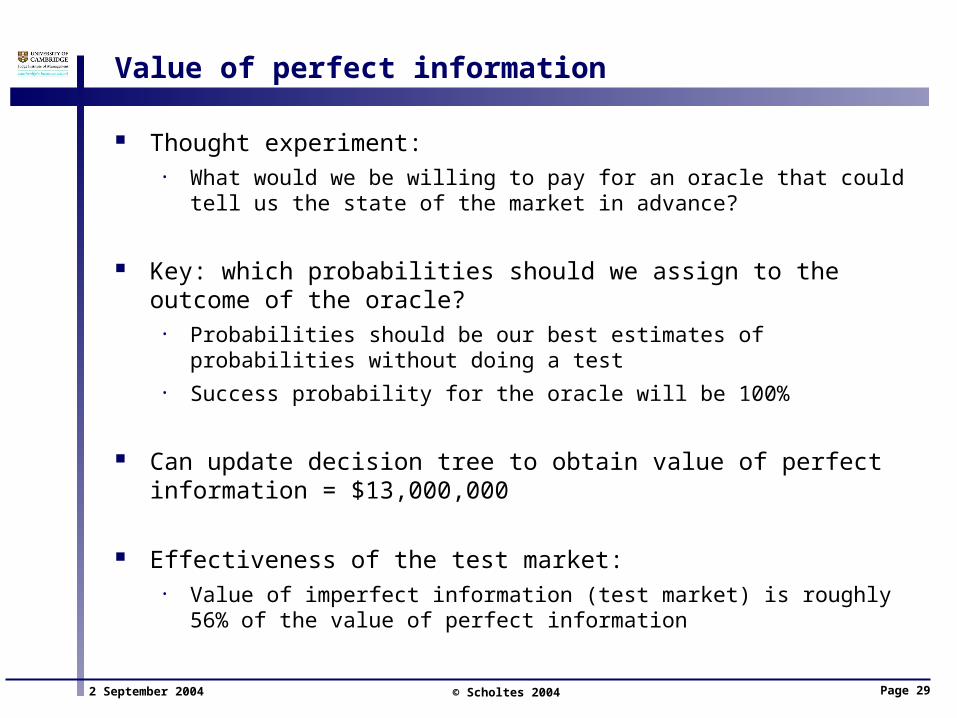
Value of perfect information

Thought experiment: • What would we be willing to pay for an oracle that could tell us the

state of the market in advance?

Key: which probabilities should we assign to the outcome of the oracle?

• Probabilities should be our best estimates of probabilities without doing a test

• Success probability for the oracle will be 100%

Can update decision tree to obtain value of perfect information = $13,000,000

Effectiveness of the test market: • Value of imperfect information (test market) is roughly 56% of the

value of perfect information


Capacity optimization

Sales projection of 5 Mio units for success scenario is due to capacity constraint

Demand for success scenario is projected to be 7 Mio units

$ 60 Mio fixed cost of production facility= $ 10 Mio fixed cost, independent of capacity+ $ 50 Mio for capacity of 5 Mio units

Variable cost of capacity is $ 10 per unit


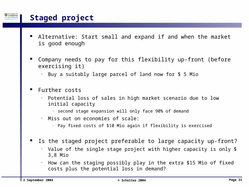
Staged project

Alternative: Start small and expand if and when the market is good enough

Company needs to pay for this flexibility up-front (before exercising it)

• Buy a suitably large parcel of land now for $ 5 Mio

Further costs• Potential loss of sales in high market scenario due to low initial

capacity T̵ second stage expansion will only face 90% of demand

• Miss out on economies of scale: T̵ Pay fixed costs of $10 Mio again if flexibility is exercised

Is the staged project preferable to large capacity up-front?• Value of the single stage project with higher capacity is only $ 3,8 Mio• How can the staging possibly play in the extra $15 Mio of fixed costs

plus the potential loss in demand?


The value of flexibility

KEY LESSON: In the presence of uncertainty managerial flexibility has considerable value

But: Managerial flexibility also costs money• E.g. buying a larger parcel of land suitable for possible later expansion

Need to trade off cost of flexibility against value of flexibility One way to quantify the value of managerial flexibility is to

compare the “value” of the “passive” project with that of the “flexible project”

• Expected value of flexibility = expected value of flexible project w/o cost of flexibility MINUS expected value of passive project

In our case: value of the passive project (with optimized capacity) = $ 4.030 M, value of the flexible project = $ 4.915 M, cost of flexibility = $ 1.000 M

Value of flexible project w/o cost of flexibility = $ 4.915M +$1.000M = $5.915 M

Value of flexibility = $5.915M - $4.030M= $1.885 M is larger than the cost of flexibility of $1.000 M


Recap Decision Analysis

MOST IMPORTANT ASPECT: DECISION TREES GIVE YOU A MODELLING TEMPLATE TO UNDERSTAND AND COMMUNICATE A DECISION PROBLEM

• Structure problem as a sequence of decisions and events

SECONDARY ASPECT: Can “optimise” decisions and value the project through “Roll-back” or “Fold-back” of the tree

KEY PROBLEM: HOW DO YOU PUT A PRICE TAG ON CHANCE NODES?


Recap Decision Analysis

Risk Profiles• Decision tree valuation using expected values assume risk

neutrality• Risk profiles provide useful additional information

Sensitivity Analysis• Probabilities and other inputs represent judgement, which includes

experience and information• Any single number is likely to be wrong

Expected value of information• The economic value of gathering more information can be

calculated before making a decision Expected value of flexibility

• The economic value of additional managerial flexibility can be incorporated into your analysis


Course content

I. IntroductionII. The forecast is always wrong

I. The industry valuation standard: Net Present Value

II. Sensitivity analysisIII. The system value is a shape

I. Value profiles and value-at-risk charts

II. SKILL: Using a shape calculatorIII. CASE: Overbooking at EasyBeds

IV. Developing valuation modelsI. Easybeds revisited

V. Designing a system means sculpting its value shapeI. CASE: Designing a Parking Garage

III. The flaw of averages: Effects of

system constraintsVI. Coping with uncertainty I:

DiversificationI. The central limit theoremII. The effect of statistical

dependenceIII. Optimising a portfolio

VII. Coping with uncertainty II: The value of information

I. SKILL: Decision Tree Analysis

II. CASE: Market Research at E-Phone

VIII. Coping with uncertainty III: The value of flexibility

Documents

Risk Management & Real Options VII. The Value of Information Stefan Scholtes Judge Institute of Management University of Cambridge MPhil Course 2004-05