1

Risk Management of Risk under the Basel Accord: Forecasting Value-at-Risk of VIX Futures*

Chia-lin Chang Department of Applied Economics

Department of Finance National Chung Hsing University

Taichung, Taiwan

Juan-Ángel Jiménez-Martín Department of Quantitative Economics

Complutense University of Madrid

Michael McAleer Econometric Institute

Erasmus School of Economics Erasmus University Rotterdam

and Tinbergen Institute The Netherlands

and Institute of Economic Research

Kyoto University, Japan

Teodosio Pérez-Amaral Department of Quantitative Economics

Complutense University of Madrid

Revised: February 2011

* The authors are most grateful for the helpful comments and suggestions of participants at the Kansai Econometrics Conference, Osaka, Japan, January 2011. For financial support, the first author acknowledges the National Science Council, Taiwan, the second and fourth authors acknowledge the Ministerio de Ciencia y Tecnología and Comunidad de Madrid, Spain, and the third author wishes to thank the Australian Research Council, National Science Council, Taiwan, and the Japan Society for the Promotion of Science.

2

Abstract

The Basel II Accord requires that banks and other Authorized Deposit-taking Institutions

(ADIs) communicate their daily risk forecasts to the appropriate monetary authorities at the

beginning of each trading day, using one or more risk models to measure Value-at-Risk

(VaR). The risk estimates of these models are used to determine capital requirements and

associated capital costs of ADIs, depending in part on the number of previous violations,

whereby realised losses exceed the estimated VaR. McAleer, Jimenez-Martin and Perez-

Amaral (2009) proposed a new approach to model selection for predicting VaR, consisting of

combining alternative risk models, and comparing conservative and aggressive strategies for

choosing between VaR models. This paper addresses the question of risk management of risk,

namely VaR of VIX futures prices. We examine how different risk management strategies

performed during the 2008-09 global financial crisis (GFC). We find that an aggressive

strategy of choosing the Supremum of the single model forecasts is preferred to the other

alternatives, and is robust during the GFC. However, this strategy implies relatively high

numbers of violations and accumulated losses, though these are admissible under the Basel II

Accord.

Key words and phrases: Median strategy, Value-at-Risk (VaR), daily capital charges, violation penalties, optimizing strategy, aggressive risk management, conservative risk management, Basel II Accord, VIX futures, global financial crisis (GFC). JEL Classifications: G32, G11, G17, C53, C22.

3

1. Introduction

Volatility derivatives have attracted much attention over the past years since they enable

trading and hedging against changes in volatility. In 1993 the Chicago Board Options

Exchange (CBOE) introduced a volatility index, VIX (Whaley, 1993), which was originally

designed to measure the market expectation of 30-day volatility implied by at-the-money

S&P100 option prices. In 2003, together with Goldman Sachs, CBOE updated VIX to reflect

a new way to measure expected volatility, one that continues to be widely used by financial

theorists.

The new VIX is based on the S&P500 Index, and estimates expected volatility by averaging

the weighted prices of S&P500 puts and calls over a wide range of strike prices. Although

many market participants considered the index to be a good predictor of short term volatility,

daily or even intraday, it took several years for the market to introduce volatility products,

starting with over the counter products such as variance swaps. The first exchange-traded

product, VIX futures, was introduced in March 2004, and was followed by VIX options in

February 2006. Both of these volatility derivatives are based on the VIX index as the

underlying asset.

This paper focuses on the VIX futures market and addresses the question of risk management

of risk when VIX futures are taken into account. McAleer, et al. (2009, 2010, 2011) analyse

from a practical perspective, how the new market risk management strategies performed

during the 2008-09 global financial crisis (GFC), and evaluate how the GFC affected the best

risk management practices. Huskaj (2009) analyzes VIX futures from a different perspective,

centered on the statistical properties of a different set of candidate forecasting models, and

without focusing on the Basel II regulations, as is considered in this paper. McAleer and

Wiphatthanananthakul (2010) examine the empirical behaviour of alternative simple expected

volatility indexes, and compare them with VIX.

The GFC of 2008-09 has left an indelible mark on economic and financial structures

worldwide, and left an entire generation of investors wondering how things could have

become so severe. There have been many questions asked about whether appropriate

regulations were in place, especially in the USA, to permit the appropriate monitoring and

encouragement of (possibly excessive) risk taking.

4

The Basel II Accord was designed to monitor and encourage sensible risk taking using

appropriate models of risk to calculate Value-at-Risk (VaR) and subsequent daily capital

charges. When the Basel I Accord was concluded in 1988, no capital requirements were

defined for market risk. However, regulators soon recognized the risks to a banking system if

insufficient capital were held to absorb the large sudden losses from huge exposures in capital

markets. During the mid-90’s, proposals were tabled for an amendment to the 1988 Accord,

requiring additional capital over and above the minimum required for credit risk. Finally, a

market risk capital adequacy framework was adopted in 1995 for implementation in 1998.

The 1995 Basel I Accord amendment provides a menu of approaches for determining market

risk capital requirements, ranging from simple to intermediate and advanced approaches.

Under the advanced approach (that is, the internal model approach), banks are allowed to

calculate the capital requirement for market risk using their internal models. The use of

internal models was introduced in 1998 in the European Union. The 26 June 2004 Basel II

framework, implemented in many countries in 2008 (though not yet in the USA), enhanced

the requirements for market risk management by including, for example, oversight rules,

disclosure, management of counterparty risk in trading portfolios.

VaR is defined as an estimate of the probability and size of the potential loss to be expected

over a given period, and is now a standard tool in risk management. It has become especially

important following the 1995 amendment to the Basel Accord, whereby banks and other

Authorized Deposit-taking Institutions (ADIs) were permitted (and encouraged) to use

internal models to forecast daily VaR (see Jorion (2000) for a detailed discussion). The last

decade has witnessed a growing academic and professional literature comparing alternative

modelling approaches to determine how to measure VaR, especially for large portfolios of

financial assets.

The amendment to the initial Basel Accord was designed to encourage and reward institutions

with superior risk management systems. A back-testing procedure, whereby actual returns are

compared with the corresponding VaR forecasts, was introduced to assess the quality of the

internal models used by ADIs. In cases where internal models lead to a greater number of

violations than could reasonably be expected, given the confidence level, the ADI is required

to hold a higher level of capital (see Table 1 for the penalties imposed under the Basel II

5

Accord). Penalties imposed on ADIs affect profitability directly through higher capital

charges, and indirectly through the imposition of a more stringent external model to forecast

VaR. This is one reason why financial managers may prefer risk management strategies that

are passive and conservative rather than active and aggressive.

Excessive conservatism can have a negative impact on the profitability of ADIs as higher

capital charges are subsequently required. Therefore, ADIs should perhaps consider a strategy

that allows an endogenous decision as to how many times ADIs should violate in any

financial year (for further details, see McAleer and da Veiga (2008a, 2008b), McAleer (2009),

Caporin and McAleer (2009b) and McAleer et al. (2009)). This paper suggests alternative

aggressive and conservative risk management strategies that can be compared with the use of

one or more models of risk throughout the estimation and forecasting periods.

This paper defines risk management in terms of choosing sensibly from a variety of risk

models, discusses the selection of optimal risk models, considers combining alternative risk

models, discusses the choice between conservative and aggressive risk management

strategies, evaluates the effects of the Basel II Accord on risk management of risk, examines

how some risk management strategies performed during the 2008-09 GFC, and evaluates how

the GFC affected risk management practices and daily capital charges.

The empirical results indicate that, when risk management is considered for VIX futures, the

optimal strategy is to be aggressive rather than conservative. Specifically, this would involve

a strategy of communicating to the national regulatory authority the Supremum of the point

forecasts of the VaR models considered. This strategy tends to minimize the average daily

capital charges, subject to staying within the limits of the number of violations that are

permitted under the Basel II Accord.

The remainder of the paper is organized as follows. In Section 2 we present the main ideas of

the Basel II Accord Amendment as it relates to forecasting VaR and daily capital charges.

Section 3 reviews some of the most well-known univariate models of conditional volatility

that are used to forecast VaR. In Section 4 the data used for estimation and forecasting are

presented. Section 5 analyses the VaR forecasts before, during and after the 2008-09 GFC.

Section 6 presents some concluding remarks.

6

2. Forecasting Value-at-Risk and Daily Capital Charges

In this section, we evaluate risk management of risk by applying the Basel II formulae to a

period that includes the 2008-09 GFC. The Basel II Accord stipulates that daily capital

charges (DCC) must be set at the higher of the previous day’s VaR or the average VaR over

the last 60 business days, multiplied by a factor (3+k) for a violation penalty, wherein a

violation involves the actual negative returns exceeding the VaR forecast negative returns for

a given day:

______

60t t-1DCC = sup - 3+ k VaR , - VaR (1)

where

DCCt = daily capital charges, which is the higher of 60

______

t-1- 3 + k VaR and - VaR ,

tVaR = Value-at-Risk for day t,

tttt zYVaR ˆ ,

60

______

VaR = mean VaR over the previous 60 working days,

tY = estimated return at time t,

tz = 1% critical value of the distribution of returns at time t,

t = estimated risk (or square root of volatility) at time t,

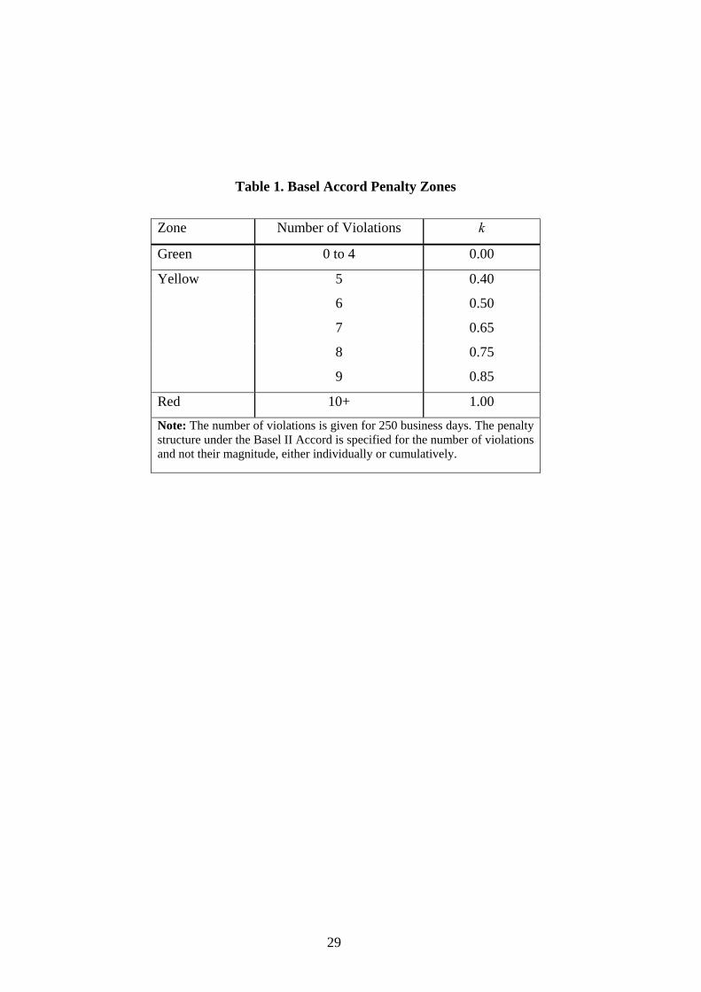
0 k 1 is the Basel II violation penalty (see Table 1).  

[Insert Table 1 here]

The formula given in equation (1) is contained in the 1995 amendment to Basel I, while Table

1 appears for the first time in the Basel II Accord in 2004.  The multiplication factor (or

penalty), k, depends on the central authority’s assessment of the ADI’s risk management

7

practices and the results of a simple backtest. It is determined by the number of times actual

losses exceed a particular day’s VaR forecast (Basel Committee on Banking Supervision

(1996, 2006)).

The minimum multiplication factor of 3 is intended to compensate for various errors that can

arise in model implementation, such as simplifying assumptions, analytical approximations,

small sample biases and numerical errors that tend to reduce the true risk coverage of the

model (see Stahl (1997)). Increases in the multiplication factor are designed to increase the

confidence level that is implied by the observed number of violations at the 99% confidence

level, as required by regulators (for a detailed discussion of VaR, as well as exogenous and

endogenous violations, see McAleer (2009), Jiménez-Martin et al. (2009), and McAleer et al.

(2010a)).

In calculating the number of violations, ADIs are required to compare the forecasts of VaR

with realised profit and loss figures for the previous 250 trading days. In 1995, the 1988 Basel

Accord (Basel Committee on Banking Supervision (1988)) was amended to allow ADIs to

use internal models to determine their VaR thresholds (Basel Committee on Banking

Supervision (1995)). However, ADIs that propose using internal models are required to

demonstrate that their models are sound. Movement from the green zone to the red zone arises

through an excessive number of violations. Although this will lead to a higher value of k, and

hence a higher penalty, violations will also tend to be associated with lower daily capital

charges. It should be noted that the number of violations in a given period is an important,

though not the only, guide for regulators to approve a given VaR model.

VaR refers to the lower bound of a confidence interval for a (conditional) mean, that is, a

“worst case scenario on a typical day”. If interest lies in modelling the random variable, Yt, it

could be decomposed as follows:

1( | )t t t tY E Y F . (2)

This decomposition states that Yt comprises a predictable component, E(Y

t| F

t1) , which is the

conditional mean, and a random component, t

. The variability of Yt

, and hence its

8

distribution, is determined by the variability of t

. If it is assumed that t follows a

conditional distribution, such that:

),(~ 2

ttt D

where t and t

are the conditional mean and standard deviation of t, respectively, these

can be estimated using a variety of parametric, semi-parametric or non-parametric methods.

The VaR threshold for Yt can be calculated as:

1( | )t t t tVaR E Y F , (3)

where is the critical value from the distribution of t to obtain the appropriate confidence

level. It is possible for t to be replaced by alternative estimates of the conditional standard

deviation in order to obtain an appropriate VaR (for useful reviews of theoretical results for

conditional volatility models, see Li et al. (2002) and McAleer (2005), where several

univariate and multivariate, conditional, stochastic and realized volatility models are

discussed).

Some recent empirical studies (see, for example, Berkowitz and O’Brien (2001), Gizycki and

Hereford (1998), and Pérignon et al. (2008)) have indicated that some financial institutions

overestimate their market risks in disclosures to the appropriate regulatory authorities, which

can imply a costly restriction to the banks trading activity. ADIs may prefer to report high

VaR numbers to avoid the possibility of regulatory intrusion. This conservative risk reporting

suggests that efficiency gains may be feasible. In particular, as ADIs have effective tools for

the measurement of market risk, while satisfying the qualitative requirements, ADIs could

conceivably reduce daily capital charges by implementing a context-dependent market risk

disclosure policy. McAleer (2009) and McAleer et al. (2010a) discuss alternative approaches

to optimize VaR and daily capital charges.

9

The next section describes several volatility models that are widely used to forecast the 1-day

ahead conditional variances and VaR thresholds.

3. Models for Forecasting VaR

ADIs can use internal models to determine their VaR thresholds. There are alternative time

series models for estimating conditional volatility. In what follows, we present several well-

known conditional volatility models that can be used to evaluate strategic market risk

disclosure, namely GARCH, GJR and EGARCH, with Gaussian, Student-t and Generalized

Normal distribution errors, where the parameters are estimated.

These models are chosen as they are widely used in the literature. For an extensive discussion

of the theoretical properties of several of these models, see Ling and McAleer (2002a, 2002b,

2003a) and Caporin and McAleer (2010b). As an alternative to estimating the parameters, we

also consider the exponential weighted moving average (EWMA) method by Riskmetrics

(1996) and Zumbauch, (2007) that calibrates the unknown parameters. We include a section

on these models to present them in a unified framework and notation, and to make explicit the

specific versions we are using. Apart from EWMA, the models are presented in increasing

order of complexity.

3.1 GARCH

For a wide range of financial data series, time-varying conditional variances can be explained

empirically through the autoregressive conditional heteroskedasticity (ARCH) model, which

was proposed by Engle (1982). When the time-varying conditional variance has both

autoregressive and moving average components, this leads to the generalized ARCH(p,q), or

GARCH(p,q), model of Bollerslev (1986). It is very common in practice to impose the widely

estimated GARCH(1,1) specification in advance.

Consider the stationary AR(1)-GARCH(1,1) model for daily returns, ty :

t 1 2 t-1 t 2y = φ +φ y + ε , φ < 1 (4)

10

for nt ,...,1 , where the shocks to returns are given by:

t t t t

2t t -1 t-1

ε = η h , η ~ iid(0,1)

h =ω+αε + βh , (5)

and 0, 0, 0 are sufficient conditions to ensure that the conditional variance

0th . The stationary AR(1)-GARCH(1,1) model can be modified to incorporate a non-

stationary ARMA(p,q) conditional mean and a stationary GARCH(r,s) conditional variance,

as in Ling and McAleer (2003b).

3.2 GJR

In the symmetric GARCH model, the effects of positive shocks (or upward movements in

daily returns) on the conditional variance, th , are assumed to be the same as the effect of

negative shocks (or downward movements in daily returns) of equal magnitude. In order to

accommodate asymmetric behaviour, Glosten, Jagannathan and Runkle (1992) proposed a

model (hereafter GJR), for which GJR(1,1) is defined as follows:

2t t -1 t -1 t-1h =ω+(α+ γI(η ))ε + βh , (6)

where 0,0,0,0 are sufficient conditions for ,0th and )( tI is an

indicator variable defined by:

1, 0

0, 0t

tt

I

(7)

as t has the same sign as t . The indicator variable differentiates between positive and

negative shocks, so that asymmetric effects in the data are captured by the coefficient . For

financial data, it is expected that 0 because negative shocks have a greater impact on risk

than do positive shocks of similar magnitude. The asymmetric effect, , measures the

11

contribution of shocks to both short run persistence, 2 , and to long run persistence,

2 .

Although GJR permits asymmetric effects of positive and negative shocks of equal magnitude

on conditional volatility, the special case of leverage, whereby negative shocks increase

volatility while positive shocks decrease volatility (see Black (1976) for an argument using

the debt/equity ratio), cannot be accommodated, in practice (for further details on asymmetry

versus leverage in the GJR model, see Caporin and McAleer (2010b)).

3.3 EGARCH

An alternative model to capture asymmetric behaviour in the conditional variance is the

Exponential GARCH, or EGARCH(1,1), model of Nelson (1991), namely:

t-1 t-1t t-1

t-1 t-1

ε εlogh =ω+α + γ + βlogh , | β |< 1

h h (8)

where the parameters , and have different interpretations from those in the

GARCH(1,1) and GJR(1,1) models.

EGARCH captures asymmetries differently from GJR. The parameters and in

EGARCH(1,1) represent the magnitude (or size) and sign effects of the standardized

residuals, respectively, on the conditional variance, whereas and represent the

effects of positive and negative shocks, respectively, on the conditional variance in GJR(1,1).

Unlike GJR, EGARCH can accommodate leverage, depending on the restrictions imposed on

the size and sign parameters, though leverage is not guaranteed.

As noted in McAleer et al. (2007), there are some important differences between EGARCH

and the previous two models, as follows: (i) EGARCH is a model of the logarithm of the

conditional variance, which implies that no restrictions on the parameters are required to

ensure 0th ; (ii) moment conditions are required for the GARCH and GJR models as they

are dependent on lagged unconditional shocks, whereas EGARCH does not require moment

conditions to be established as it depends on lagged conditional shocks (or standardized

12

residuals); (iii) Shephard (1996) observed that 1|| is likely to be a sufficient condition for

consistency of QMLE for EGARCH(1,1); (iv) as the standardized residuals appear in equation

(7), 1|| would seem to be a sufficient condition for the existence of moments; and (v) in

addition to being a sufficient condition for consistency, 1|| is also likely to be sufficient

for asymptotic normality of the QMLE of EGARCH(1,1).

The three conditional volatility models given above are estimated under the following

distributional assumptions on the conditional shocks: (1) Gaussian, (2) Student-t, with

estimated degrees of freedom, and (3) Generalized Normal. As the models that incorporate the

t distributed errors are estimated by QMLE, the resulting estimators are consistent and

asymptotically normal, so they can be used for estimation, inference and forecasting.

3.4 Exponentially Weighted Moving Average (EWMA)

As an alternative to estimating the parameters of the appropriate conditional volatility models,

Riskmetrics (1996) developed a model which estimates the conditional variances and

covariances based on the exponentially weighted moving average (EWMA) method, which is,

in effect, a restricted version of the ARCH( ) model. This symmetric approach forecasts the

conditional variance at time t as a linear combination of the lagged conditional variance and

the squared unconditional shock at time 1t . The EWMA model calibrates the conditional

variance as:

2t t-1 t-1h = λh +(1- λ)ε (9)

where is a decay parameter. Riskmetrics (1996) suggests that should be set at 0.94 for

purposes of analysing daily data. As no parameters are estimated, there are no moment or log-

moment conditions.

13

14

4. Data

The data used in estimation and forecasting are closing daily prices (settlement prices) for the

30-day maturity CBOE VIX volatility index futures (ticker name VX), and were obtained

from the Thomson Reuters-Data Stream Database for the period 26 March 2006 to 10 January

2011. The settlement price is calculated by the CBOE as the average of the closing bid and

ask quote so as to reduce the noise due to any microstructure effects. The contracts are cash

settled on the Wednesday 30 days prior to the third Friday on the calendar month immediately

following the month in which the contract expires. The underlying asset is the VIX index that

was originally introduced by Whaley (1993) as an index of implied volatility on the S&P100.

In 2003 the new VIX was introduced based on the S&P500 index.

VIX is a measure of the implied volatility of 30-day S&P500 options. Its calculation is

independent of an option pricing model and is calculated from the prices of the front month

and next-to-front month S&P500 at-the-money and out-the-money call and put options. The

level of VIX represents a measure of the implied volatilities of the entire smile for a constant

30-day to maturity option chain. VIX is quoted in percentage points (for example, 30.0 VIX

represents an implied volatility of 30.0%). In order to invest in VIX, an investor can take a

position in VIX futures or VIX options.

Although VIX represents a measure of the expected volatility of the S&P500 over the next

30-days, the prices of VIX futures are based on the current expectation of what the expected

30-day volatility will be at a particular time in the future (on the expiration date). Although

the VIX futures should converge to the spot at expiration, it is possible to have significant

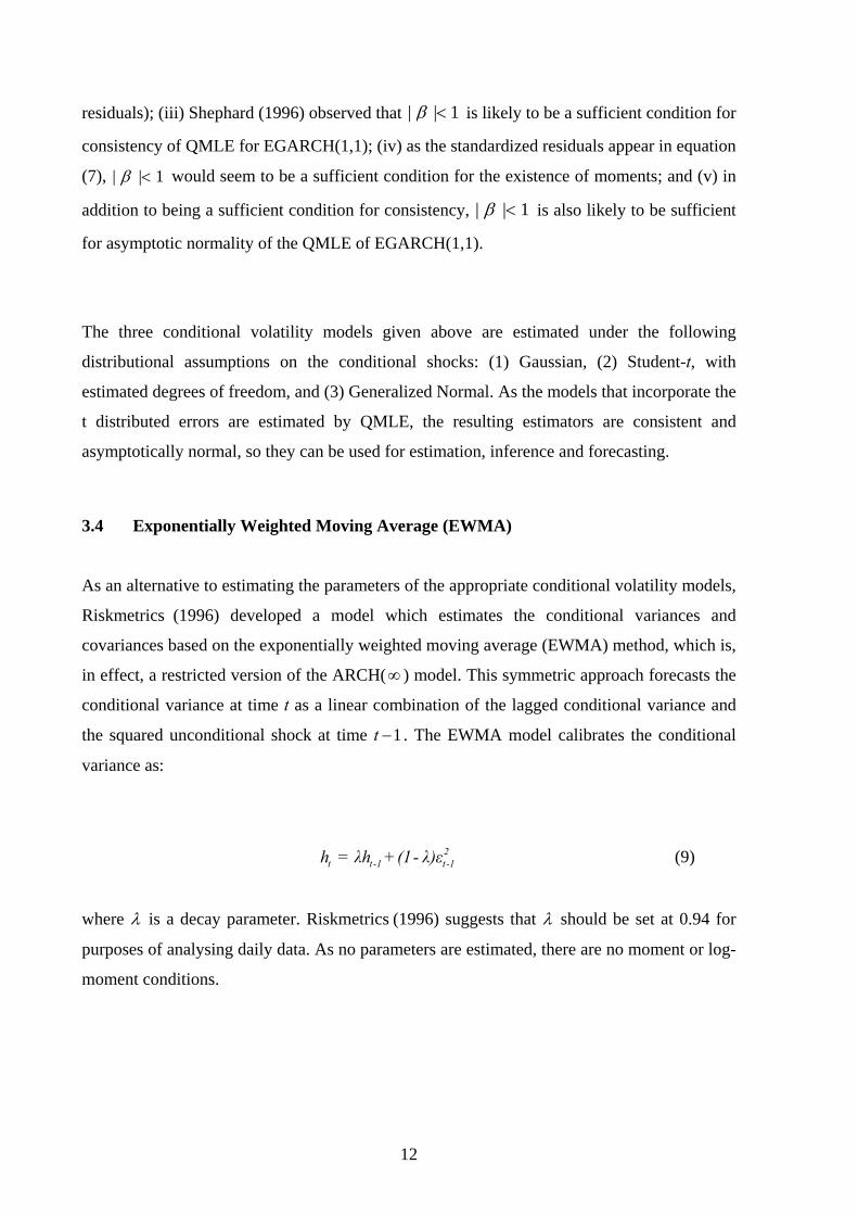
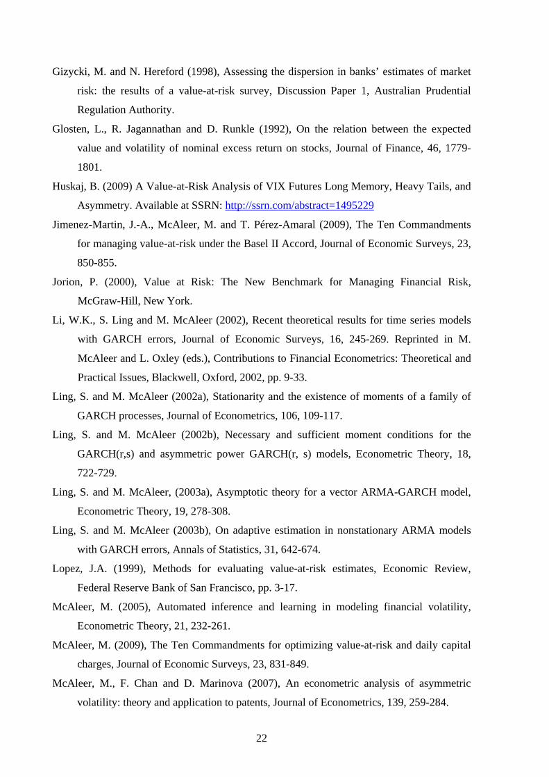
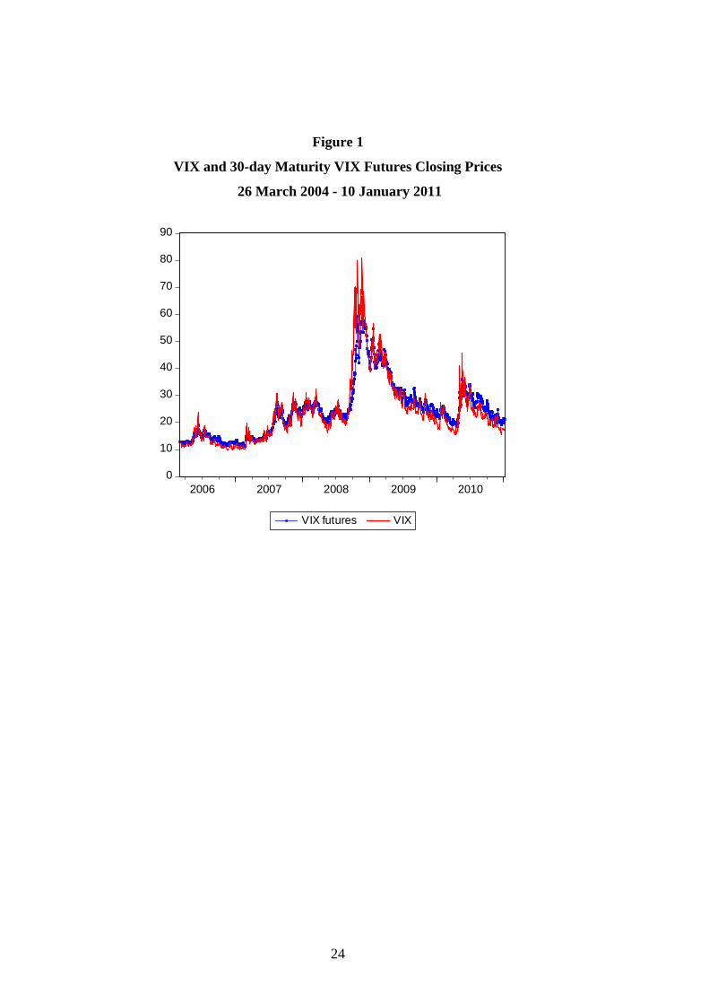
disparities between the spot VIX and VIX futures prior to expiration. Figure 1 shows the daily

VIX futures index together with the 30 day maturity VIX futures closing prices. VIX has a

correlation (0.96) with the 30-day maturity VIX futures. Regarding volatility, VIX futures

prices tend to show significantly lower volatility than VIX, which can be explained by the fact

that VIX futures must be priced in a manner that reflects the mean reverting nature of VIX.

For the whole sample, the standard deviation is 11.12 for VIX and 9.55 for VIX futures

prices.

In Figure 1 it can be seen that, from 2004 until 2007, the equity markets enjoyed a tranquil

period, as did the VIX futures prices. After the first signs of a looming economic crisis, VIX

15

futures rose sharply, in July 2007, after fluctuating around an average of 14. Following the

Lehman Brothers collapse in September 2008, VIX futures appeared to jump to an all time

high of over 66.23 in November 20, 2008. VIX futures prices returned to around $20 in 2009,

but with the Greek crisis in May 2010, the VIX futures prices again jumped to around $36.

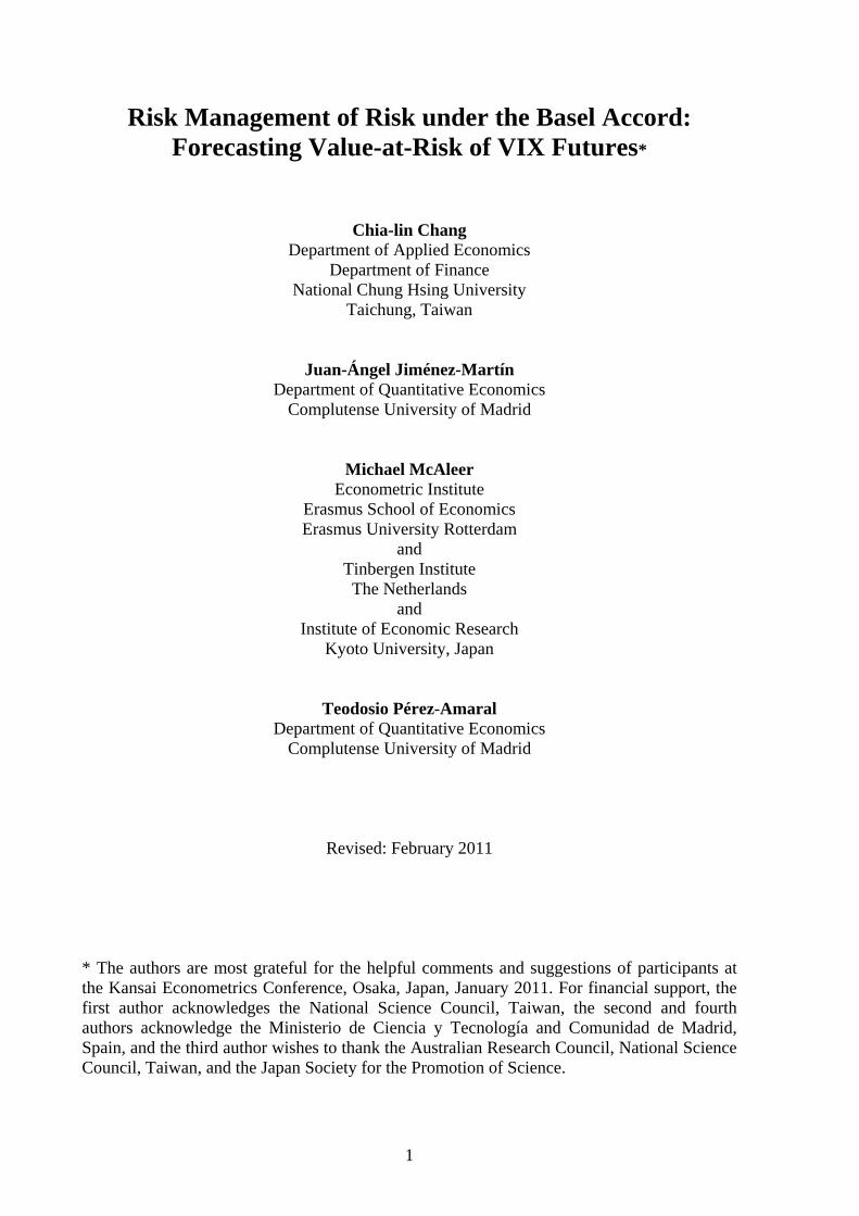
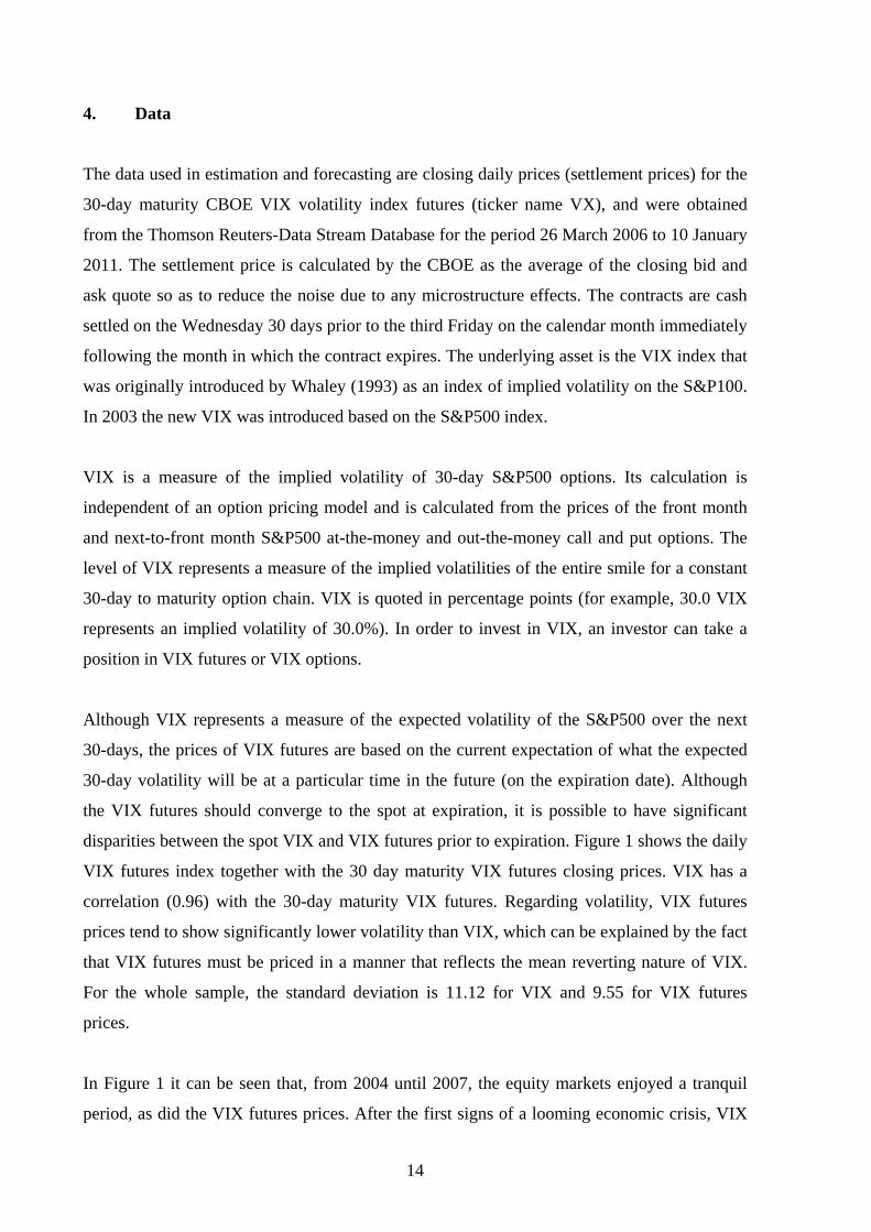
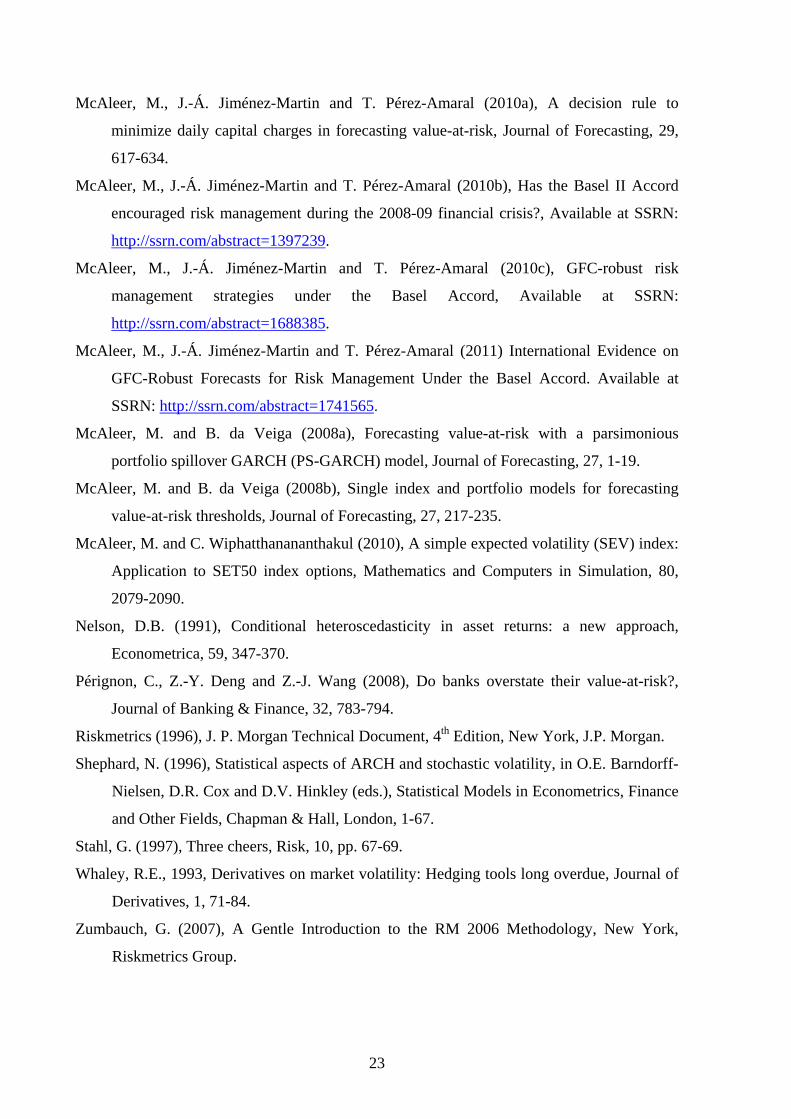
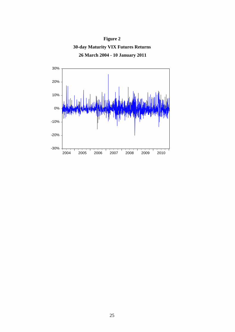
If tP denotes the closing prices of the VIX futures contract at time t, the returns at time t ( )tR

are defined as:

1100*log / t t tR P P . (10)

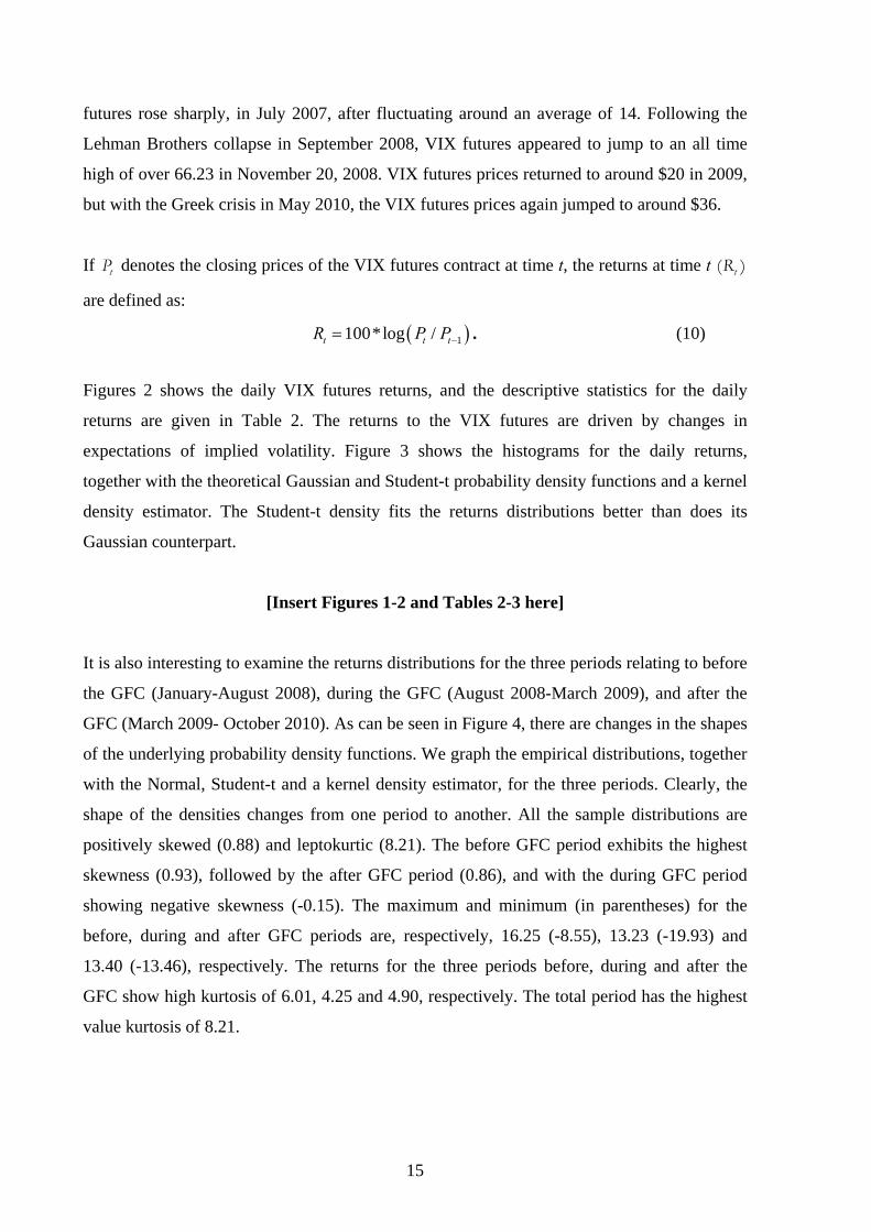
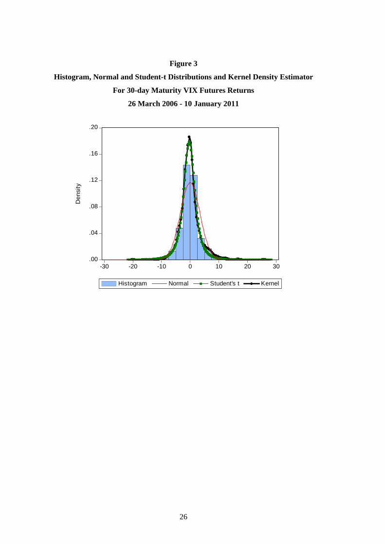
Figures 2 shows the daily VIX futures returns, and the descriptive statistics for the daily

returns are given in Table 2. The returns to the VIX futures are driven by changes in

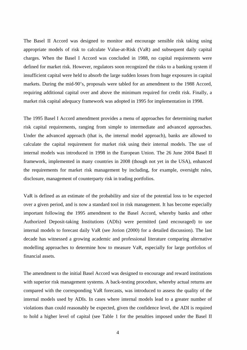
expectations of implied volatility. Figure 3 shows the histograms for the daily returns,

together with the theoretical Gaussian and Student-t probability density functions and a kernel

density estimator. The Student-t density fits the returns distributions better than does its

Gaussian counterpart.

[Insert Figures 1-2 and Tables 2-3 here]

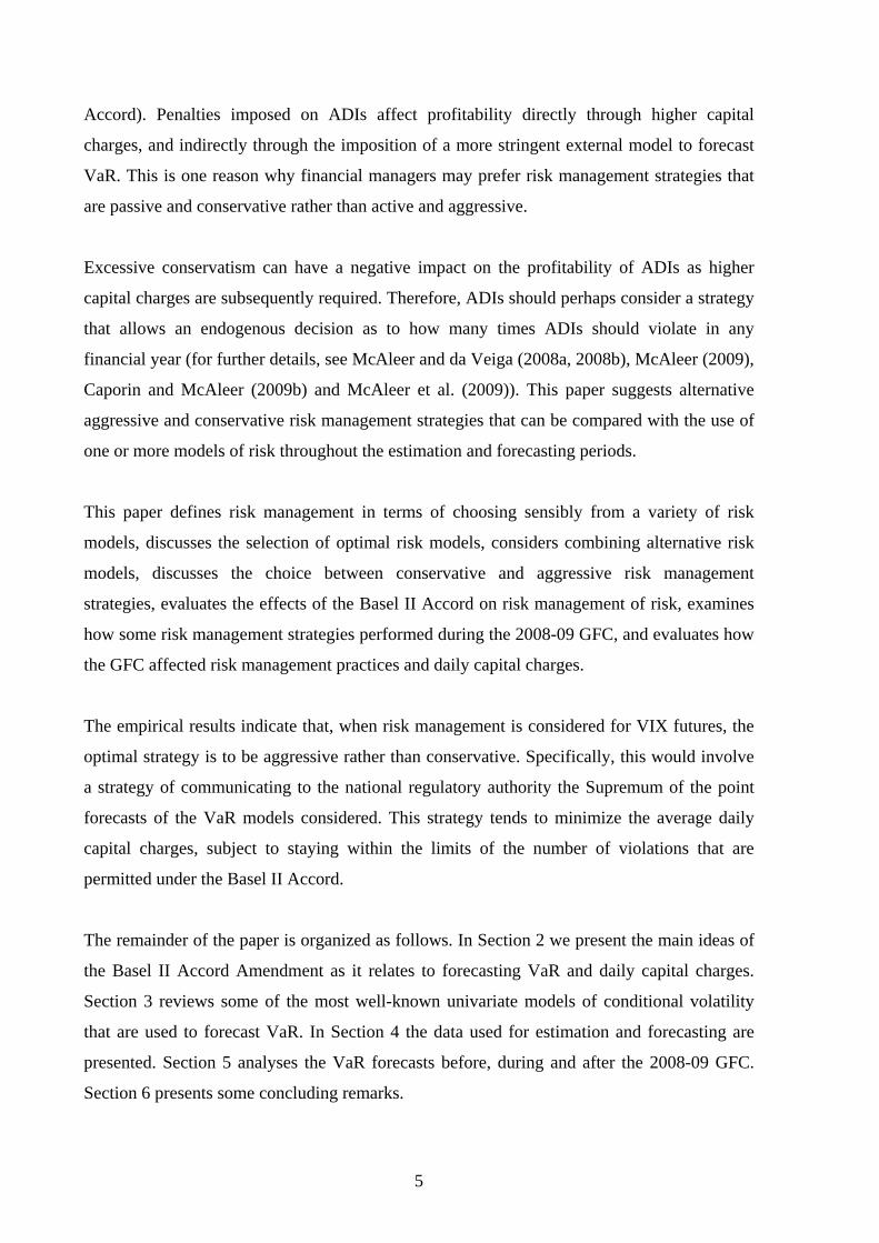
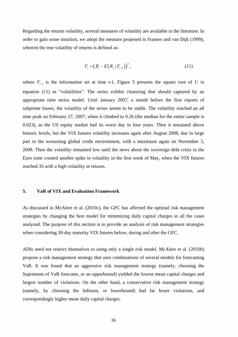
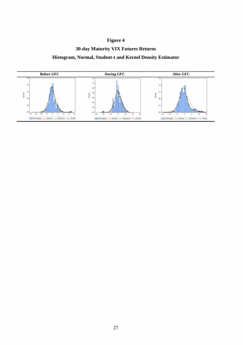
It is also interesting to examine the returns distributions for the three periods relating to before

the GFC (January-August 2008), during the GFC (August 2008-March 2009), and after the

GFC (March 2009- October 2010). As can be seen in Figure 4, there are changes in the shapes

of the underlying probability density functions. We graph the empirical distributions, together

with the Normal, Student-t and a kernel density estimator, for the three periods. Clearly, the

shape of the densities changes from one period to another. All the sample distributions are

positively skewed (0.88) and leptokurtic (8.21). The before GFC period exhibits the highest

skewness (0.93), followed by the after GFC period (0.86), and with the during GFC period

showing negative skewness (-0.15). The maximum and minimum (in parentheses) for the

before, during and after GFC periods are, respectively, 16.25 (-8.55), 13.23 (-19.93) and

13.40 (-13.46), respectively. The returns for the three periods before, during and after the

GFC show high kurtosis of 6.01, 4.25 and 4.90, respectively. The total period has the highest

value kurtosis of 8.21.

16

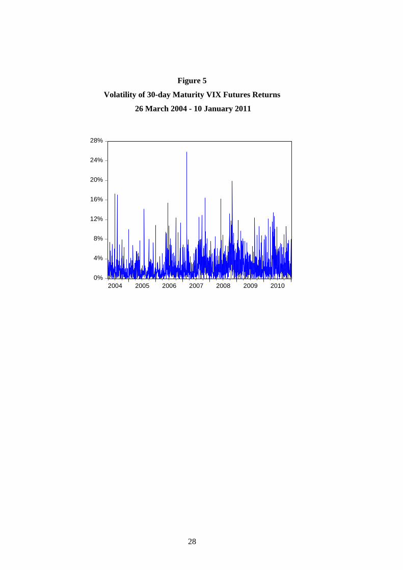
Regarding the returns volatility, several measures of volatility are available in the literature. In

order to gain some intuition, we adopt the measure proposed in Franses and van Dijk (1999),

wherein the true volatility of returns is defined as:

2

1| t t t tV R E R F , (11)

where 1tF is the information set at time t-1. Figure 5 presents the square root of Vt in

equation (11) as “volatilities”. The series exhibit clustering that should captured by an

appropriate time series model. Until January 2007, a month before the first reports of

subprime losses, the volatility of the series seems to be stable. The volatility reached an all

time peak on February 27, 2007, when it climbed to 0.26 (the median for the entire sample is

0.023), as the US equity market had its worst day in four years. Then it remained above

historic levels, but the VIX futures volatility increases again after August 2008, due in large

part to the worsening global credit environment, with a maximum again on November 3,

2008. Then the volatility remained low until the news about the sovereign debt crisis in the

Euro zone created another spike in volatility in the first week of May, when the VIX futures

reached 35 with a high volatility in returns.

5. VaR of VIX and Evaluation Framework

As discussed in McAleer et al. (2010c), the GFC has affected the optimal risk management

strategies by changing the best model for minimizing daily capital charges in all the cases

analyzed. The purpose of this section is to provide an analysis of risk management strategies

when considering 30-day maturity VIX futures before, during and after the GFC.

ADIs need not restrict themselves to using only a single risk model. McAleer et al. (2010b)

propose a risk management strategy that uses combinations of several models for forecasting

VaR. It was found that an aggressive risk management strategy (namely, choosing the

Supremum of VaR forecasts, or an upperbound) yielded the lowest mean capital charges and

largest number of violations. On the other hand, a conservative risk management strategy

(namely, by choosing the Infinum, or lowerbound) had far fewer violations, and

correspondingly higher mean daily capital charges.

17

McAleer et al. (2010c) forecast VaR using ten single GARCH-type models with different

error distributions. Additionally, they analyze twelve new strategies based on combinations of

the previous standard single-model forecasts of VaR, namely: Infinum (0th percentile),

Supremum (100th percentile), Average, Median and nine additional strategies based on the

10th through to the 90th percentiles. This is intended to select a robust VaR forecast,

irrespective of the time period, that provides reasonable daily capital charges and number of

violation penalties under the Basel Accord. They found that the Median (50th percentile) is a

GFC-robust strategy, in the sense that maintaining the same risk management strategy before,

during and after the GFC leads to comparatively low daily capital charges and violation

penalties under the Basel Accord.

In this section, we conduct a similar exercise to analyze the risk management performance of

existing VaR forecasting models, as permitted under the Basel II framework, when applied to

VIX futures prices.

5.1 Evaluating Risk Management Strategies

In Table 3 the performance criteria are calculated for each model and error distribution, and

for each of the three sub-samples: before, during, and after the 2008-09 GFC. Based on the

S&P500 peaks and troughs, before the GFC is prior to 11 August 2008, during the GFC is

from 12 August 2008 through to 9 March 2009, and after the GFC is from 10 March 2009

onwards.

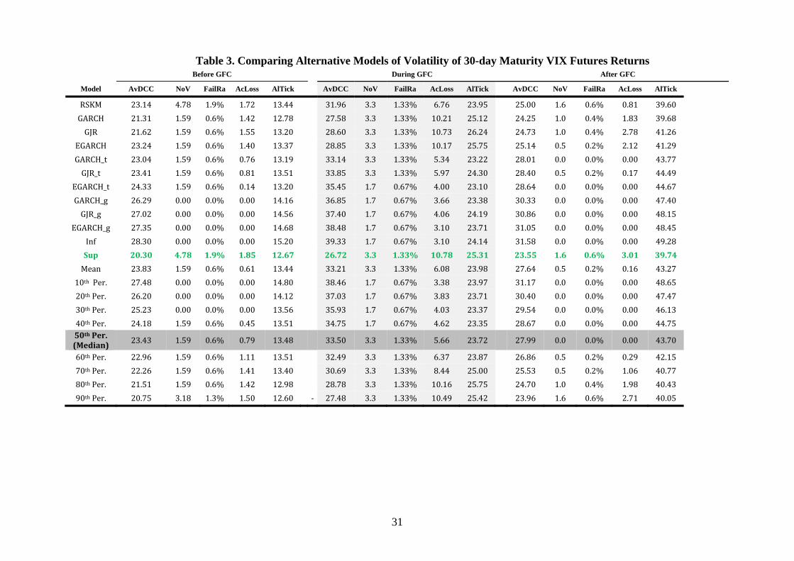
Table 3 shows the values of the criteria used for comparison of the strategies for forecasting

the volatility and VaR of the VIX futures returns. The first column indicates the name of the

model or combination of models that are used. The first row marks three groups of five

columns each, corresponding to before, during and after the GFC. Each of the three groups of

columns contains the average daily capital charges (AvDCC), the normalized number of

violations, (NoV), failure rate (FailRa), accumulated losses, (AcLoss) and asymmetric linear

tick loss function (AlTick) that are obtained by each strategy in each of the three periods

related to the GFC.

18

Our basic criterion for choosing a strategy is minimizing the average daily capital charges

subject to the constraint that the normalized number of violations (equivalently, the

percentage of violations) is within the limits allowed under the Basel II Accord. Additionally,

we consider the accumulated losses, which are not taken into account in the rules of Basel II,

but which might be considered in the future. In principle, low values of this criterion are

desirable. We also consider the asymmetric loss tick function, which should be minimized.

The main conclusions can be summarized as follows:

1. Before the GFC, the best strategy for minimizing daily capital charges (DCC) is the

Supremum. It has the lowest AvDCC (20.30) and the highest number of violations

(4.78), but is still within the limits of the Basel II Accord. The Supremum also has the

next to lowest asymmetric linear tick loss function (12.67). However, it also has the

highest accumulated losses (1.85). The Supremum is clearly the best strategy for

forecasting the VaR of VIX futures before the GFC.

2. During the GFC, the Supremum has the lowest average daily capital charges (26.72)

and highest (but admissible) number of violations (3.3). Moreover, it has one of the

three lowest values of the AlTick (25.31). However, the Supremum shows the highest

accumulated losses of all the models (25.31). In general, the Supremum is the optimal

strategy for managing risk under the Basel II Accord during the GFC.

3. After the GFC, the Supremum has the lowest average daily capital charges (23.55), at

the cost of the highest (but admissible) number of violations (1.6). Moreover, the

Supremum has one of the three lowest asymmetric linear tick loss function values

(39.74), at the cost of the highest accumulated losses (3.01).

The Supremum emerges as the optimal strategy for minimizing daily capital charges, at a cost

in terms of the number of violations, and accumulated losses which are permissible under the

Basel II Accord.

A comparison with a leading competitor, Riskmetrics, which is shown in the first row of

Table 3, reveals that the Supremum consistently dominates Riskmetrics. The Supremum

19

always has lower daily capital charges, with the same number of violations, across all the time

periods that are considered, namely before, during and after the GFC.

In summary, the Supremum is the risk management strategy that performs the best across all

the considered strategies and time periods. It is also a GFC-robust strategy, as defined in

McAleer et al. (2010c, 2011), meaning it is an optimal strategy that is valid before, during and

after the GFC.

6. Conclusion

In the spectrum of financial assets, VIX futures prices are a relatively new financial product.

As with any financial asset, VIX futures are subject to risk. In this paper we analyzed the

performance of a variety of strategies for managing the risk, through forecasting VaR, of VIX

futures under the Basel II Accord, before, during and after the global financial crisis (GFC) of

2008-09.

We forecast VaR using well known univariate model strategies, as well as new strategies

based on combinations of risk models, that were proposed and analyzed in McAleer et al.

(2009, 2010c, 2011).

The candidate strategies for forecasting VaR of the VIX futures, and for managing risk under

the Basel II Accord, were several univariate models, such as Riskmetrics, GARCH, EGARCH

and GJR, each subject to different error distributions. We also used several more sophisticated

strategies that combined single models, such as the Supremum, Infinum, Average, Median

and the 10th through 90th percentiles of the point values of the forecasts of the univariate

models.

Our main criterion for choosing between strategies is minimizing the average daily capital

charges subject to the constraint that the number of violations (equivalently, the percentage of

violations) is within the limits allowed by the Basel II Accord. Additionally, we consider the

accumulated losses and asymmetric loss tick function, each of which would desirably have

low values.

20

The principal empirical conclusions of the paper can be summarized as follows:

1. Before the GFC, the Supremum has the lowest Average Daily Capital Charges

(AvDCC) (20.30) and the highest (though admissible) number of violations (4.78)

under the Basel II Accord.

2. During the GFC, the Supremum has the lowest AvDCC (26.72) and highest (but

admissible) number of violations (3.3).

3. After the GFC, the Supremum has the lowest AvDCC (23.55), at the cost of the

highest (but admissible) number of violations (1.6).

The Supremum dominates Riskmetrics consistently as it always has lower daily capital

charges, with the same number of violations across all time periods: before, during and after

the GFC.

The attraction for risk managers in using the Supremum strategy is that they do not need to

keep changing the rules for generating daily VaR forecasts. The Supremum is an aggressive

and profitable risk strategy for calculating VaR forecasts for VIX futures, both in tranquil and

in turbulent times.

The idea of combining different VaR forecasting models is entirely within the spirit of the

Basel Accord, although its use would require approval by the regulatory authorities, as for any

forecasting model. This approach is not at all computationally demanding, even though

several models need to be specified and estimated over time.

21

References

Basel Committee on Banking Supervision, (1988), International Convergence of Capital

Measurement and Capital Standards, BIS, Basel, Switzerland.

Basel Committee on Banking Supervision, (1995), An Internal Model-Based Approach to

Market Risk Capital Requirements, BIS, Basel, Switzerland.

Basel Committee on Banking Supervision, (1996), Supervisory Framework for the Use of

“Backtesting” in Conjunction with the Internal Model-Based Approach to Market Risk

Capital Requirements, BIS, Basel, Switzerland.

Basel Committee on Banking Supervision, (2006), International Convergence of Capital

Measurement and Capital Standards, a Revised Framework Comprehensive Version,

BIS, Basel, Switzerland.

Berkowitz, J. and J. O’Brien (2001), How accurate are value-at-risk models at commercial

banks?, Discussion Paper, Federal Reserve Board.

Black, F. (1976), Studies of stock market volatility changes, in 1976 Proceedings of the

American Statistical Association, Business & Economic Statistics Section, pp. 177-181.

Bollerslev, T. (1986), Generalised autoregressive conditional heteroscedasticity, Journal of

Econometrics, 31, 307-327.

Borio, C. (2008), The financial turmoil of 2007-?: A preliminary assessment and some policy

considerations, BIS Working Papers No 251, Bank for International Settlements, Basel,

Switzerland.

Caporin, M. and M. McAleer (2010a), The Ten Commandments for managing investments,

Journal of Economic Surveys, 24, 196-200.

Caporin, M. and M. McAleer (2010b), Model selection and testing of conditional and

stochastic volatility models, to appear in L. Bauwens, C. Hafner and S. Laurent (eds.),

Handbook on Financial Engineering and Econometrics: Volatility Models and Their

Applications, Wiley, New York (Available at SSRN: http://ssrn.com/abstract=1676826).

Chicago Board Options Exchange, (2003), VIX: CBOE volatility index, Working paper,

Chicago.

Engle, R.F. (1982), Autoregressive conditional heteroscedasticity with estimates of the

variance of United Kingdom inflation, Econometrica, 50, 987-1007.

Franses, P.H. and D. van Dijk (1999), Nonlinear Time Series Models in Empirical Finance,

Cambridge, Cambridge University Press.

22

Gizycki, M. and N. Hereford (1998), Assessing the dispersion in banks’ estimates of market

risk: the results of a value-at-risk survey, Discussion Paper 1, Australian Prudential

Regulation Authority.

Glosten, L., R. Jagannathan and D. Runkle (1992), On the relation between the expected

value and volatility of nominal excess return on stocks, Journal of Finance, 46, 1779-

1801.

Huskaj, B. (2009) A Value-at-Risk Analysis of VIX Futures Long Memory, Heavy Tails, and

Asymmetry. Available at SSRN: http://ssrn.com/abstract=1495229

Jimenez-Martin, J.-A., McAleer, M. and T. Pérez-Amaral (2009), The Ten Commandments

for managing value-at-risk under the Basel II Accord, Journal of Economic Surveys, 23,

850-855.

Jorion, P. (2000), Value at Risk: The New Benchmark for Managing Financial Risk,

McGraw-Hill, New York.

Li, W.K., S. Ling and M. McAleer (2002), Recent theoretical results for time series models

with GARCH errors, Journal of Economic Surveys, 16, 245-269. Reprinted in M.

McAleer and L. Oxley (eds.), Contributions to Financial Econometrics: Theoretical and

Practical Issues, Blackwell, Oxford, 2002, pp. 9-33.

Ling, S. and M. McAleer (2002a), Stationarity and the existence of moments of a family of

GARCH processes, Journal of Econometrics, 106, 109-117.

Ling, S. and M. McAleer (2002b), Necessary and sufficient moment conditions for the

GARCH(r,s) and asymmetric power GARCH(r, s) models, Econometric Theory, 18,

722-729.

Ling, S. and M. McAleer, (2003a), Asymptotic theory for a vector ARMA-GARCH model,

Econometric Theory, 19, 278-308.

Ling, S. and M. McAleer (2003b), On adaptive estimation in nonstationary ARMA models

with GARCH errors, Annals of Statistics, 31, 642-674.

Lopez, J.A. (1999), Methods for evaluating value-at-risk estimates, Economic Review,

Federal Reserve Bank of San Francisco, pp. 3-17.

McAleer, M. (2005), Automated inference and learning in modeling financial volatility,

Econometric Theory, 21, 232-261.

McAleer, M. (2009), The Ten Commandments for optimizing value-at-risk and daily capital

charges, Journal of Economic Surveys, 23, 831-849.

McAleer, M., F. Chan and D. Marinova (2007), An econometric analysis of asymmetric

volatility: theory and application to patents, Journal of Econometrics, 139, 259-284.

23

McAleer, M., J.-Á. Jiménez-Martin and T. Pérez-Amaral (2010a), A decision rule to

minimize daily capital charges in forecasting value-at-risk, Journal of Forecasting, 29,

617-634.

McAleer, M., J.-Á. Jiménez-Martin and T. Pérez-Amaral (2010b), Has the Basel II Accord

encouraged risk management during the 2008-09 financial crisis?, Available at SSRN:

http://ssrn.com/abstract=1397239.

McAleer, M., J.-Á. Jiménez-Martin and T. Pérez-Amaral (2010c), GFC-robust risk

management strategies under the Basel Accord, Available at SSRN:

http://ssrn.com/abstract=1688385.

McAleer, M., J.-Á. Jiménez-Martin and T. Pérez-Amaral (2011) International Evidence on

GFC-Robust Forecasts for Risk Management Under the Basel Accord. Available at

SSRN: http://ssrn.com/abstract=1741565.

McAleer, M. and B. da Veiga (2008a), Forecasting value-at-risk with a parsimonious

portfolio spillover GARCH (PS-GARCH) model, Journal of Forecasting, 27, 1-19.

McAleer, M. and B. da Veiga (2008b), Single index and portfolio models for forecasting

value-at-risk thresholds, Journal of Forecasting, 27, 217-235.

McAleer, M. and C. Wiphatthanananthakul (2010), A simple expected volatility (SEV) index:

Application to SET50 index options, Mathematics and Computers in Simulation, 80,

2079-2090.

Nelson, D.B. (1991), Conditional heteroscedasticity in asset returns: a new approach,

Econometrica, 59, 347-370.

Pérignon, C., Z.-Y. Deng and Z.-J. Wang (2008), Do banks overstate their value-at-risk?,

Journal of Banking & Finance, 32, 783-794.

Riskmetrics (1996), J. P. Morgan Technical Document, 4th Edition, New York, J.P. Morgan.

Shephard, N. (1996), Statistical aspects of ARCH and stochastic volatility, in O.E. Barndorff-

Nielsen, D.R. Cox and D.V. Hinkley (eds.), Statistical Models in Econometrics, Finance

and Other Fields, Chapman & Hall, London, 1-67.

Stahl, G. (1997), Three cheers, Risk, 10, pp. 67-69.

Whaley, R.E., 1993, Derivatives on market volatility: Hedging tools long overdue, Journal of

Derivatives, 1, 71-84.

Zumbauch, G. (2007), A Gentle Introduction to the RM 2006 Methodology, New York,

Riskmetrics Group.

24

Figure 1

VIX and 30-day Maturity VIX Futures Closing Prices

26 March 2004 - 10 January 2011

0

10

20

30

40

50

60

70

80

90

2006 2007 2008 2009 2010

VIX futures VIX

25

Figure 2

30-day Maturity VIX Futures Returns

26 March 2004 - 10 January 2011

-30%

-20%

-10%

0%

10%

20%

30%

2004 2005 2006 2007 2008 2009 2010

26

Figure 3

Histogram, Normal and Student-t Distributions and Kernel Density Estimator

For 30-day Maturity VIX Futures Returns

26 March 2006 - 10 January 2011

.00

.04

.08

.12

.16

.20

-30 -20 -10 0 10 20 30

Histogram Normal Student's t Kernel

Den

sity

27

Figure 4

30-day Maturity VIX Futures Returns

Histogram, Normal, Student-t and Kernel Density Estimator

Before GFC During GFC After GFC

.00

.04

.08

.12

.16

.20

-20 -15 -10 -5 0 5 10 15 20

Histogram Normal Student's t Kernel

De

nsi

ty

.00

.02

.04

.06

.08

.10

.12

.14

-30 -20 -10 0 10 20 30

Histogram Normal Student's t Kernel

De

nsi

ty

.00

.04

.08

.12

.16

.20

-15 -10 -5 0 5 10 15

Histogram Normal Student's t Kernel

De

nsi

ty

28

Figure 5

Volatility of 30-day Maturity VIX Futures Returns

26 March 2004 - 10 January 2011

0%

4%

8%

12%

16%

20%

24%

28%

2004 2005 2006 2007 2008 2009 2010

29

 

Table 1. Basel Accord Penalty Zones

Zone Number of Violations k

Green 0 to 4 0.00

Yellow 5 0.40

6 0.50

7 0.65

8 0.75

9 0.85

Red 10+ 1.00

Note: The number of violations is given for 250 business days. The penalty structure under the Basel II Accord is specified for the number of violations and not their magnitude, either individually or cumulatively.

30

Table 2 30-day Maturity VIX Futures Returns: Histogram and Descriptive Statistics

26 March 2004 - 10 January 2011

0

100

200

300

400

500

600

700

-20 -10 0 10 20

Series: VIX FuturesSample 26/03/2004 10/01/2011Observations 1771

Mean 0.001859Median -0.210453Maximum 25.81866Minimum -19.92871Std. Dev. 3.412287Skewness 0.882711Kurtosis 8.210094

Jarque-Bera 2233.068Probability 0.000000

31

Table 3. Comparing Alternative Models of Volatility of 30-day Maturity VIX Futures Returns Before GFC During GFC After GFC

Model AvDCC NoV FailRa AcLoss AlTick AvDCC NoV FailRa AcLoss AlTick AvDCC NoV FailRa AcLoss AlTick

RSKM  23.14  4.78  1.9%  1.72  13.44    31.96  3.3  1.33%  6.76  23.95    25.00  1.6  0.6%  0.81  39.60 GARCH  21.31  1.59  0.6%  1.42  12.78    27.58  3.3  1.33%  10.21  25.12    24.25  1.0  0.4%  1.83  39.68 GJR  21.62  1.59  0.6%  1.55  13.20    28.60  3.3  1.33%  10.73  26.24    24.73  1.0  0.4%  2.78  41.26 

EGARCH  23.24  1.59  0.6%  1.40  13.37    28.85  3.3  1.33%  10.17  25.75    25.14  0.5  0.2%  2.12  41.29 GARCH_t  23.04  1.59  0.6%  0.76  13.19    33.14  3.3  1.33%  5.34  23.22    28.01  0.0  0.0%  0.00  43.77 GJR_t  23.41  1.59  0.6%  0.81  13.51    33.85  3.3  1.33%  5.97  24.30    28.40  0.5  0.2%  0.17  44.49 

EGARCH_t  24.33  1.59  0.6%  0.14  13.20    35.45  1.7  0.67%  4.00  23.10    28.64  0.0  0.0%  0.00  44.67 GARCH_g  26.29  0.00  0.0%  0.00  14.16    36.85  1.7  0.67%  3.66  23.38    30.33  0.0  0.0%  0.00  47.40 GJR_g  27.02  0.00  0.0%  0.00  14.56    37.40  1.7  0.67%  4.06  24.19    30.86  0.0  0.0%  0.00  48.15 

EGARCH_g  27.35  0.00  0.0%  0.00  14.68    38.48  1.7  0.67%  3.10  23.71    31.05  0.0  0.0%  0.00  48.45 Inf  28.30  0.00  0.0%  0.00  15.20    39.33  1.7  0.67%  3.10  24.14    31.58  0.0  0.0%  0.00  49.28 Sup  20.30  4.78  1.9%  1.85  12.67      26.72  3.3  1.33%  10.78  25.31    23.55  1.6  0.6%  3.01  39.74 

Mean  23.83  1.59  0.6%  0.61  13.44    33.21  3.3  1.33%  6.08  23.98    27.64  0.5  0.2%  0.16  43.27 10th  Per.  27.48  0.00  0.0%  0.00  14.80    38.46  1.7  0.67%  3.38  23.97    31.17  0.0  0.0%  0.00  48.65 20th Per.  26.20  0.00  0.0%  0.00  14.12    37.03  1.7  0.67%  3.83  23.71    30.40  0.0  0.0%  0.00  47.47 30th Per.  25.23  0.00  0.0%  0.00  13.56    35.93  1.7  0.67%  4.03  23.37    29.54  0.0  0.0%  0.00  46.13 40th Per.  24.18  1.59  0.6%  0.45  13.51    34.75  1.7  0.67%  4.62  23.35    28.67  0.0  0.0%  0.00  44.75 50th Per. (Median) 

23.43  1.59  0.6%  0.79  13.48      33.50  3.3  1.33%  5.66  23.72    27.99  0.0  0.0%  0.00  43.70 

60th Per.  22.96  1.59  0.6%  1.11  13.51    32.49  3.3  1.33%  6.37  23.87    26.86  0.5  0.2%  0.29  42.15 70th Per.  22.26  1.59  0.6%  1.41  13.40    30.69  3.3  1.33%  8.44  25.00    25.53  0.5  0.2%  1.06  40.77 80th Per.  21.51  1.59  0.6%  1.42  12.98    28.78  3.3  1.33%  10.16  25.75    24.70  1.0  0.4%  1.98  40.43 90th Per.  20.75  3.18  1.3%  1.50  12.60  ‐ 27.48  3.3  1.33%  10.49  25.42    23.96  1.6  0.6%  2.71  40.05