132 DOE 76-45\11

SSDC:~ 1 Revision I

RISK MANAGEMENT GUIDE

EG&G Idaho. Inc

P 0 Box 1625 Idaho Falls. Idaho 83415

September 1982

UNITED STATES

D E P A R T M E N T OF E N E R G Y Offtce of the Deputy Assistant

Secretary for Environment Safe* and Health

This document contains new concepts or the author(s) interpretation of new calculationsand/or measurements; accordingly, EG&G Idaho, Inc. is required by the United States Government to include the following disclaimer:

I DISCLAIMER I This report was prepared as an account of work sponsored by an agency of the United States Government. Neither the United Slates Government nor an" m m c v ~ ~ ~ ~~ ~ ~ ~ ~ ~ - ~ - ~ ~ - ~ ~~ , ---..-, thereof, nor any of their employees, makes any warranty, express or implied, or assumes any legal liability or responsibility for the accuracy, completeness, or usefulness of any information, apparatus, product or process disclosed, or represents that its use would not infringe privately owned rights. References herein to any specific commercial product, process, or service bytrade name, trademark, manufacturer, or otherwise, does not necessarily constitute or imply its endorsement, recommendation, or favoring by the United States Government orany agency thereof. The views and opinions of authors expressed herein do not necessarily state or reflect those of the United States Government or any agency thereof.

Available from:

System Safe ty Development Center EG&G Idaho, Inc. P . 0 . Box 1625 Idaho F a l l s , Idaho 83401

R I S K MANAGEMENT GUIDE

Prepared by

Glen J. Br i scoe

System Safe ty Development Center EG&G Idaho, Inc .

Idaho F a l l s , Idaho 83415

September 1982

FOREWORD

This Guide presents an expansion of the risk discussion in the

Management Oversight Risk Tree Analysis ~anua1.l'~ It was prepared as a textbook for use in Risk Analysis Workshops for Department of Energy

personnel and for safety staffs of Department of Energy contractors.

The discussion includes the risk analysis of operational accidents and

the role of risk analysis in line management and safety functions.

Elementary probability, statistics, and risk theory are given. Practical

applications for safety professionals and line managers are also given.

Line managers will be able to determine the necessary elements for a

comprehensive risk management or 105s control program. In addition, safety

professionals will be able to apply basic risk evaluation techniques to new

or existing systems, ranging from a single operation or process to an entire

project or company.

Engineering analysis techniques (such as fault tree analysis or consequence analysis) and the processes of integrating risk with other organizational factors leading to managerial decisions are outside the

scope of this Guide.

CONTENTS

FOREWORD .............................................................. ii

GLOSSARY .............................................................. v

INTRODUCTION .................................................... SUMMARY .........................................................

...................................................... BACKGROUND

3.1 Unders tand ing R i s k ........................................ 3.2 R i s k P e r c e p t i o n ........................................... RISK MANAGEMENT ................................................. REPORT TO MANAGEMENT ............................................ ANALYTICAL METHODS FOR RISK QUANTIFICATION ...................... 6.1 A c t u a r i a l R i s k Assessment ................................. 6.2 Example Problem ........................................... 6.3 S u b j e c t i v e R i s k Es t ima te .................................. 6.4 Survey Methods ............................................ 6.5 I nsu rance R i s k ............................................ 6.6 L i f e Sho r t en ing E f f e c t s ................................... 6.7 Trend A n a l y s i s ............................................ 6.8 Log-Normal D i s t r i b u t i o n ................................... 6.9 Extreme Value A n a l y s i s .................................... 6.10 F a u l t T ree A n a l y s i s and O the r Hazard I d e n t i f i c a t i o n

and E v a l u a t i o n Techniques ................................. CONSEQUENCE ANALYSIS ............................................ 7.1 D i r e c t and I n d i r e c t Acc i den t Cos ts ........................ 7.2 D i r e c t Acc i den t Cos ts .....................................

7.2.1 F i r s t Aid. On-S i te Med i ca l ........................ 7.2.2 O f f - S i t e Med i ca l ..................................

..................................... 7.2.3 Workdays Los t

iii

7.2.4 F a t a l i t y C o s t s .................................... 6 8 ................................... 7.2.5 P r o p e r t y Damage 70

............................................ 7.3 I n d i r e c t C o s t s 7 1

............................... 7.3.1 I n j u r e d Worker T ime 71 7.3.2 Co-worker Time .................................... 71

................................... 7.3.3 S u p e r v i s o r Time 72 7.3.4 G e n e r a l Losses .................................... 72

RISK ASSESSMENT OF EXISTING SYSTEMS ............................. 75

8.1 Genera l ................................................... 75

8.2 R i s k I d e n t i f i c a t i o n and Rank ing ........................... 75

8.3 T h e o r e t i c a i R i s k .......................................... 80

RISK ASSESSMENT OF NEW SYSTEMS .................................. BY

9.1 Resource A l l o c a t i o n ....................................... Yo

REFERENCES ...................................................... 105

BIBILOGRAPHY .................................................... 107

APPENDIX A.. RISK IDENTIFICATION TREE .................................. A-1

APPENDIX 0- USE OF RISK PROJECTION TECHNIQUES I N INVESTIGATION OF ACCIDENTS AND INCIDENTS ........................ 8 - 2

APPENDIX C.. PROBABILITY AND STATISTICS PRIMER ......................... C-1

APPENDIX &-PLOTTING METHODS. GOODNESS-OF-FIT TESTING. AND CONFIDENCE L IMITS FOR LOG-NORMAL AND EXTREME VALUE DATA ......... 0-1

APPENDIX E- RISK ASSESSMENT EXAMPLES ................................. E-1

RISK MANAGEMENT G U I D E

Frequent ly , management a l l o c a t e s s i g n i f i c a n t resources t o c o r r e c t

s p e c i f i c hazards w i t h o u t f i r s t o b t a i n i n g s u f f i c i e n t i n f o r m a t i o n t o determine

whether more hazardous c o n d i t i o n s a re be ing neglected, o r whether t h e co r -

r e c t i v e cos t s a re j u s t i f i e d by t h e b e n e f i t o r t h e r e d u c t i o n i n r i s k . I n

a d d i t i o n , management f r e q u e n t l y has l i t t l e o r no i n fo rma t i on of how r i s k

compares t o t h e a c t u a l va lue of a g i ven program, and thus must make many

s a f e t y - r e l a t e d dec i s i ons w i t h o u t s u f f i c i e n t in format ion .

The Management Ove rs igh t R i sk Tree (MORT) methodology p rov ides a system

f o r i d e n t i f y i n g management o v e r s i g h t s and s p e c i f i c r i s k s . Once r i s k s have

been i d e n t i f i e d , i t i s t hen management's r e s p o n s i b i l i t y t o p rov ide r e q u i r e d

resources t o reduce o r e l i m i n a t e s p e c i f i c r i s k s and t o assume t h e r e s i d u a l

r i s k s .

R i s k assessment es t ima tes o f f u t u r e l osses and t h e e f f ec t i veness o f

a d d i t i o n a l c o n t r o l s p rov ides management i n f o r m a t i o n t o make sound dec i s i ons

rega rd ing r i s k . indeed, knowledge of r i s k p e r m i t s t h e respons ib le person

t o dec ide whether a danger can be accepted, must be reduced, o r e l i m i n a t e d

b y a p p l i c a t i o n of a d d i t i o n a l p r o t e c t i v e measures, o r whether t h e o p e r a t i o n

must be cance l l ed .

AS such, r i s k management and assessment i s bas i c t o a system approach

t o sa fe t y management.

S p e c i f i c a l l y , r i s k assessment p e r m i t s o r p rov ides :

1. P r o b a b i l i t y es t ima tes o f l a r g e o r c a t a s t r o p h i c acc idents .

2. A d d i t i o n o f such l o s s es t ima tes a c t u a r i a l p r e d i c t i o n s of l o s s t o

p r o v i d e a more complete r i s k es t imate .

3. Making sa fe t y programs more c o s t e f f e c t i v e by concen t ra t i ng on

h i g h r i s k areas.

4. Optimization of the combined cost of safety programs and the cost

of accidents which present at a given level of control. This

includes selection of the list of the various alternatives

regarding specific hazards and control measures.

5. Evaluation of the effects of codes, standards, and regulations

and the need for relaxation or additional controls.

6. Consideration of various types of risk on a consistent basis minimizing the effects of emotions, fears, and personalities with

regard to such related subjects as low probability, high conse-

quence events, environmental and health issues, and immediate

versus latent effects.

Various types and degrees of danger are thus treated objectively with

biases minimized.

Thus, the role of risk assessment is to provide the necessary informa-

tion to make decisions regarding the cost effective commitment of resources

to accident prevention and reduction. Risk assessment can also be used to determine if a proposed action is acceptable in those situations where it

is impractical to eliminate particular hazards. Obviously, those areas

where the greatest gains can be made with the least effort should be given

top priority. Such prioritization will effect the greatest safety with any

given level of effort.

A limitation in this process is that estimates of future losses are necessarily based on probabilities, statistics, and even subjective judg-

ment; and therefore can never be precise. The decision to allocate

resources, thus, is always made in the face of uncertainty. The purpose of

risk analysis is to reduce that uncertainty as much as practical by provid-

ing a framework for the incorporation of all available information regarding

the costs and risks of various alternatives. This guide provides some

methods for analyzing and presenting this data to management.

2. SUMMARY

R i s k a n a l y s i s i s t h e s c i e n t i f i c measurement of t h e degree of danger o r

hazard i n v o l v e d i n any o p e r a t i o n o r a c t i v i t y . More p r e c i s e l y i t i s a prod-

u c t of t h e frequency and s e v e r i t y of unwanted o r acc iden ta l events. Mea-

surements of t h e f requency o f unplanned events can never be p r e c i s e and

t h e r e f o r e i n v o l v e va r i ous degrees of u n c e r t a i n t y . I n a d d i t i o n , adverse

consequences i n v o l v e a g r e a t v a r i e t y of p r imary adverse e f f e c t s and many

secondary e f f ec t s . The t a n g i b l e e f f ec t s i n c l u d e degradat ion of t h e env i ron -

ment, l a t e n t h e a l t h e f f e c t s f o r b o t h t h e p u b l i c and employees, p r o p e r t y

damage, v e h i c l e acc idents , and many secondary e f f e c t s such as reduced

environmental values, programmatic delays, e tc . As such, t h e assessment o f

r i s k i s n o t s imple and r e q u i r e s a wide range of knowledge. The v e r y com-

p l e x i t y and l a c k of unders tand ing o f r i s k leads t o gross misconcept ions.

Many v e r y low r i s k s a re pe rce i ved as ex t reme ly r i s k y and v i c e versa.

S c i e n t i f i c d a t a c o l l e c t i o n , ana lys is , and p r e p a r a t i o n of r e s u l t s can do

much t o p r o v i d e an unders tand ing of r i s k and t o p r o v i d e management w i t h an

es t ima ted probab le c o s t o f acc iden ts i n an o p e r a t i o n o r a c t i v i t y and t h e

u n c e r t a i n t y i n t h a t es t ima te i n c l u d i n g t h e range of s e v e r i t y and

p r o b a b i l i t y .

W i th t h i s i n fo rma t i on , management can make sound dec i s i ons r e l a t e d t o

a l l o c a t i o n of sa fe t y resources. Th i s systems approach t o sa fe t y , o r r i s k

management i nc ludes t h e f o l l o w i n g s teps:

1. Es tab l ishment of company p o l i c y , s e t t i n g of acceptab le o r upper

l i m i t s of r i s k , and s e t t i n g goa ls f o r r e d u c t i o n o f r i s k

2. Determinat ion of r i s k th rough r i s k assessment and a n a l y s i s of

hazards

3. A l l o c a t i o n of resources t o c o n t r o l t h e q u a n t i f i e d r i s k below t h e

upper l i m i t s and t o achieve t h e r i s k goa ls

4. Acceptance of r e s i d u a l r i s k o r losses which a re expected t o occur

a t t h e s p e c i f i e d c o n t r o l l e v e l

5. Monitoring the operation and safety program for change to assure continuance of acceptable levels of safety.

The risk analysis collect and analyze risk data and prepare reports

which permit the manager to fulfill his functions in the above risk manage-

ment steps. To prepare usefull reports, the exact purpose or expected use

of information must be clearly understood and stated. Assumptions must be

distinguished from facts. Not only the results but the analytical methods must be clear and consise.

A large number of analytical methods are available for the risk analyst. The simplest is the direct use of actuarial data (accident

statistics).

Last year's losses are the simplest most direct estimate of next

year's expected loss or risk. Basic probability and statistical methods

can provide knowledge regarding the range and uncertainty of these future

losses and add meaning to accident statistics normally presented to

management.

In the absence of data, subjective estimates may be required or a

survey conducted. Properly made, these provide risk information that is

far superior to hunches or pure guessing. Collection, analysis, and use of

these actuarial and subjective data are very similar to that of the insur-

ance industry; long-term average losses must be estimated and precautions

made for not only the average loss but also for the unusual year in which

an extremely large loss occurs.

Predictability and identification of these large losses enhances the

ability to prevent them. Such information can be gained through graphical

analysis of the frequency-severity relationship of accidents. Two methods

for doing this are the log-normal and extreme value analyses.

Not only do these methods permit prediction of large losses, but they

also provide insights into safety management. A relatively large number of

midrange accidents compared to smaller accidents indicates either or both

under reporting of small losses and inadequate systems for control of large

losses.

The different types of losses present a risk assessment problem in that there are no standard common units in which to sum different types of

risk. Either techniques which thinly disguise placing a dollar value on

the environment, health, or on human life, or a direct dollar value must be assumed if comparisons between various types of risk and subsequent

equitable allocation of resources are to be made.

In the assessment of loss of human life, the loss is greater for

accidents which occur more frequently at younger ages and latent health

effects which result in fatalities later in life. This difference can be

accounted for by stating the risk in terms of years-of-life lost rather

than by the number of premature fatalities.

Finally, a number of methods are available for summarizing the various kinds of loss in order to provide an overview of company risks. Neglect of

one dissipline or concentrating too much in another can thus be identified

and rectified. Use of these methods will place safety programs in a sound

objective basis and will provide the greatest amount of safety for a given

budget line. Human life is far too valuable, injuries far too painful,

property damage and delays far too costly to do otherwise.

3. BACKGROUND

Risk evaluation has its origins in probability theory and statistics.

The first formulation of probability theory was made by Pascal in the

17th century in order to evaluate gambling risks. Today, games of chance, such as dice and roulette, are used as examples of probability theory. In 1713, about a half century later, Bernoulli developed what is called the

Bernoulli theorem of binomial distribution. This theory is useful in deal- ing not only with games of chance but also with quality control, inspection,

public opinion polling, genetics, etc.

Later, Poisson developed basic theory dealing with how often events

occur. If more than one event can occur per trial, it determines the proba-

bility that " x " events will occur. For example, what is the probability of a given number of counts on a Geiger counter in a 15-8 interval, the number of worms in a cubic foot of soil, or the number of accidents in a given

period of time?

It appears that the first application of probability mathematics to

accident frequency or risk evaluation was by Von Bortkiewiczl in the 19th century. He studied the records of soldiers dying from kicks of horses in 20 Prussian Army Corps over a period of 10 years. For these 200 sets of observations, he calculated the relative frequency with 0, 1, 2, 3, or

4 deaths would occur and compared the results to actual experience. In one instance there were four deaths even though the average was only 0.6 deaths.

The calculations were in good agreement and Von Bortkiewicz concluded there

was no evidence that in any one corps in any given year, soldiers were more

careless or horses were more wild.

The lesson for the safety engineer is that if a "rash" of accidents

occur, it is not easy to determine whether changes have occurred causing an

increase in accident frequency or whether the rash is a rare, random

situation such as when four soldiers were kicked to death in a single year in one corps.

Near the end of the 18th century, Gauss developed the theory of normal

or Gaussian distribution. This theory deals with continuous rather than

t h e d i s c r e t e d i s t r i b u t i o n of t h e B e r n o u l l i ( b i n o m i a l ) and Poisson t h e o r i e s .

F o r example, t h e e a r l i e r t h e o r i e s p r e d i c t t h a t an event w i l l o r w i l l n o t

happen ( two p o s s i b i l i t i e s ) ; thus, t h e te rm b inomia l . The Gaussian t h e o r y

approximates d i s t r i b u t i o n s of measurements i n nature, i n d u s t r y , psychology,

e t c . F o r example, what f r a c t i o n of t h e s tudents i n a c lassroom a re i n a

g i ven weight o r h e i g h t range, r a t h e r t han s imp ly d e a l i n g w i t h how f r e q u e n t l y

an event w i l l occur. Th i s t h e o r y can a l s o p r e d i c t t h e probab le number o f

acc iden ts which w i l l occur i n a g i ven t ime per iod .

R i sk e v a l u a t i o n was nex t app l i ed by t h e insurance i n d u s t r y . U n t i l

r ecen t l y , t h e i r approach t o r i s k e v a l u a t i o n has been s t r i c t l y a c t u a r i a l o r

s t a t i s t i c a l . (Based on p a s t exper ience, what are t h e expected losses n e x t

yea r? ) T h e i r approach t o t h e q u a n t i f i c a t i o n of r i s k has been t o develop

i n c r e a s i n g l y complex and narrower c l asses o f r i s k . P re fe r red r i s k premiums

apply, f o r example, t o b u i l d i n g s w i t h f i r e p r o t e c t i o n systems, peop le who

do n o t smoke, a d u l t s w i t h no teenage d r i v e r s , e t c . Where exper ience has

been l a c k i n g t o p r e d i c t f u t u r e losses, insurance companies have p r o t e c t e d

themselves by v e r y l a r g e premiums and/or by l i m i t a t i o n s o f l i a b i l i t y . These

a re n o t v i a b l e o p t i o n s f o r t h e program manager, t he re fo re he needs g r e a t e r

r i s k assessment c a p a b i l i t y .

The f i r s t n a t i o n a l t a b u l a t i o n of work acc iden ts and r a t e s was pub l i shed

i n Acc ident Fac ts by t h e Na t i ona l Safe ty Counc i l i n 1928. Safe ty eng ineers

soon began s t a t i s t i c a l a n a l y s i s of acc idents . I n t h e 19308, H e i n r i c h

s t u d i e d acc iden t f requency and s e v e r i t y and concluded t h a t f o r each

300 m ino r i n j u r i e s t h e r e were 30 se r i ous i n j u r i e s and 1 f a t a l i t y . Whi le

these s t a t i s t i c s may rep resen t t h e average throughout a l l i ndus t r y , t h e i r

use cou ld be m is lead ing and dangerous. For example, t h e e s t i m a t i o n of t h e

p r o b a b i l i t y o f a f a t a l i t y based on these s t a t i s t i c s and t h e number of

i n j u r i e s i n an o f f i c e may l ead t o undue concern and s a f e t y e f f o r t s .

Obviously, we cannot p r e d i c t t h e chance of a f a t a l i t y based on paper cu t s ,

f i n g e r s shu t i n drawers, e t c . On t h e o t h e r hand, no h i g h r i s e c o n s t r u c t i o n

worker should t ake comfort i n t h e f a c t t h e r e had been few m ino r i n j u r i e s

among h i s coworkers.

The first large attempt to analyze and control hazards was with the Manhattan project. Previously, new technology was developed with practi-

cally no safety considerations in the design or development stages. Steam- boat explosions were common on the Mississippi River in the 19th century.

In the 19308, the automobile death rate per vehicle mile, even at the lower

speeds, was nearly three times the current rate. Countless eyes were need- lessly lost before the need for safety glasses was realized.

However, beginning with the Manhattan project, the nuclear industry

introduced safety analysis reports, safe work permits, etc. Each phase of

each project was routinely and systematically analyzed for hazards, and

control measures were adopted prior to starting the actual work.

These original safety analyses were limited to identification of

hazards and evaluation of maximum consequences (worst-case analysis). The

safety analysis reports were primarily concerned with limiting the worst

accident (the Maximum Hypothetical Accident, later called the Design Basis

Accident) to a given consequence level. For example, the risk was con-

sidered acceptable if the off-site radiation dose from the maximum credible

accident did not exceed specified limits. The risks of more frequent but

smaller accidents were treated superficially or not at all. The identifi-

cation of hazards usually resulted in control measures being applied with-

out cost/benefit analysis (risk quantification).

2 In the 19508, Gumbel developed the extreme value theory which can

be used to predict the frequency of maximum events. This theory was first

applied to natural events such as maximum river flow, highest winds, etc.

The theory was also used to determine the adequacy of dams and flood control

projects, the necessary wind resistance capabilities of building structures,

etc.

With the development of intercontinental missiles equipped with nuclear

warheads, a major advance in risk evaluation was necessary. An unplanned

or inadvertent release of a nuclear missile programmed for the destruction

of a foreign city was beyond any previously conceived or actual accident. i

No previous experience was available to apply statistical theory. A search

f o r ways t h e acc iden t c o u l d happen and a p p r o p r i a t e coun te r measures (as was

done i n t h e n u c l e a r i n d u s t r y ) was necessary b u t inadequate. A sys temat ic

method f o r e v a l u a t i n g t h e p r o b a b i l i t y f o r i n a d v e r t e n t m i s s i l e launch was

needed. As a r e s u l t , f a u l t t r e e t h e o r y was developed.

I n f a u l t t r e e ana l ys i s , a s i n g l e event (such as t h e a c c i d e n t a l r e l e a s e

o f a m i s s i l e ) i s pos tu la ted . Then, d i f f e r e n t events which can l ead t o t h i s

acc iden t are searched f o r and arranged i n a diagram which resembles a

" t r e e . ' Th i s process i s cont inued u n t i l i n d i v i d u a l component f a i l u r e o r

i n i t i a t i n g human e r r o r i s reached. The t r e e arrangement p e r m i t s sequence

of events and f a i l u r e r e l a t i o n s h i p s and consequences t o be eva luated.

Assignment of p r o b a b i l i t i e s of i n i t i a t i n g events i n t h e f a u l t t r e e p e r m i t s

t h e e v a l u a t i o n of p r o b a b i l i t y p ropaga t i on t o t h e t o p event. As f a r as

p o s s i b l e o r p r a c t i c a l , a l l p o s s i b l e pa ths l ead ing t o t h e t o p event a r e

i d e n t i f i e d ; and t h e p ropaga t i on o f consequence up th rough t h e t r e e f rom t h e

m u l t i t u d e o f i n d i v i d u a l component f a i l u r e s and human e r r o r s a re analyzed by

t h e use of p r o b a b i l i t y theory . Thus, t h e l i k e l i h o o d o f t h e t o p event ( o r

0 acc iden t ) can be es t imated. O f perhaps g r e a t e r va lue i s t h a t t h e va r i ous

cha ins of events which can l ead t o t h e t o p event a r e i d e n t i f i e d , and add i -

t i o n a l systems c o n t r o l can be app l i ed where most needed.

The a p p l i c a t i o n of p r o b a b i l i t y ( f r equency -seve r i t y ) d i s t r i b u t i o n s t o

i n d u s t r i a l acc iden ts has been developed r e c e n t l y . Gumbel's extreme va lue

a n a l y s i s cou ld have p r e d i c t e d t h a t a l a r g e f i r e had a r e l a t i v e l y h i g h

p r o b a b i l i t y o f o c c u r r i n g a t Rocky F l a t s . Th i s techn ique i s c u r r e n t l y be ing

used t o c a l c u l a t e t h e f requency o f maximum acc iden ts i n c l u d i n g f i r e s . The

log-normal d i s t r i b u t i o n , a s p e c i a l i z e d case o f t h e genera l Gaussian o r

normal d i s t r i b u t i o n , has been used t o p l o t t h e f requency and s e v e r i t y of

acc iden ts and t o p r e d i c t t h e f requency of l a r g e events. Such p r e d i c t i o n s

a r e g e n e r a l l y i n good agreement w i t h extreme va lue theory . They have t h e

added advantage o f i n c l u d i n g a l l acc idents , n o t j u s t t h e wors t acc iden t i n

each t ime pe r i od . As such, t h e log-normal d i s t r i b u t i o n can be i n t e g r a t e d

t o q u a n t i f y t h e e n t i r e spectrum o f acc idents . For example, t h e log-normal

p l o t i s e x t r a p o l a t e d t o i n c l u d e t h e l a r g e events which may be under repre-

sented i n t h e h i s t o r i c a l data. The i n t e g r a t i o n t hen i nc ludes t h e e n t i r e

spectrum of acc iden ts . Whi le t h e p r o b a b i l i t y o f t h e maximum o r worst-case

accidents can be reduced to acceptable levels with fault tree analysis, this

technique provides some assurance that the sum total costs of all accidents

will be within tolerable levels.

Yet to be developed are standard values for different kinds of risk

(life, property environment, etc.). Also in the formative stage are stan- dards for risk acceptability and resource allocation. Currently the science and use of risk assessment and management is growing rapidly. Many com- panies now have a position of risk manager. The Federal Government now requires risk cost/benefit studies for proposed regulations to reduce

hazards. Insurance companies are becoming aware that more sophisticated

risk assessment techniques are needed. It is hoped that this report will provide assistance for DOE and its contractors who wish to begin or improve an existing risk assessment and/or management program.

3.1 Understanding Risk

Laplace wrote in 1814, "Strictly speaking, it may be said that nearly

all of our knowledge is problematical." Thus, managers and safety officials (in fact everyone in all matters of life) make decisions based on evidence

which is logically incomplete.

The amount and quality of evidence available to predict a given outcome

determines the confidence or degree of assurance in the likely outcome and

Provides a measure of probability of given outcome. As evidence changes, our confidence in the outcome or our estimate of the probability of the

outcome changes. Thus, probability is not an intrinsic characteristic or

trait of a future event but only a measure of evidence for that event.

Thus, consideration of probability whether quantified or intuitive plays a

fundamental role in rational thought and conduct, and has been declared to

be the guide of life.

Estimates of probability may be very precise, as in the probability of

a five in a single throw of a die as 1/6, or very imprecise as in proba-

bility of a given return on a stock investment. In neither case does an estimation or probability influence the outcome. In every individual

trial, regardless of the probability and regardless of how accurately that

probability is known, the proposed event will either occur or not occur.

An estimate on a subjective probability is a measurement of how strong

the estimator feels about a situation. While this may vary from individual

to individual, the uncertainty can be reduced by using a panel of experts

andlor by averaging subjective estimates. Incorporation of such feelings

(numerically) into a risk analysis is better than no analysis and also

serves to document or record differences of opinion. Indeed, it provides a

record of estimates for the risk evaluation, which can be changed, if desired; and new results can then be calculated. In such cases, the chief

value of risk analysis may not be the final risk figures obtained, which

are certain to be open to much criticism and questioning. The value will lie in revealing many, if not most, of the various possible damage causing

mechanisms; and thereby provide better insights to effective control

measures.

Thus probability can be defined as (a) a measure of subjective expecta-

tion, (b ) a degree of confidence in an outcome whose numerical value can be

estimated by logical reasoning, and (c) the relative frequency with which

any event occurs in a class of events.

In a broad sense, risk refers to the uncertainty in any outcome. Risk management and assessment includes assembly, analysis, and use of knowledge

in a systematic way to define and reduce the uncertainty in any outcome

whether associated with danger to personnel and property or not.

This guide is limited to the narrow concept of risk which deals with

the danger of loss from accidents. As explained in more detail later, risk

is defined as the probability of loss multiplied by a measure of the consequence.

There is an element of danger in every human activity. Usually, people try to avoid danger and take all due precautions to preserve life

and limb. Yet there is an element of intrigue and excitement in risk

taking. The death defying high wire acts and other stunts where daredevils

deliberately flirt with death attract crowds and much public attention. In spite of the fact that risk is common and all live with it everyday, when

it comes to evaluating and understanding risk, many feel there is a mystique

about the unfamiliar subject of risk. Indeed, many are prone to say of a

fatal accident that "his time had come." Nevertheless, the concept of risk

is quite simple. The dictionary defines risk as "the chance (probability) of harm or adverse consequences" or as "the degree of exposure to loss or

injury." These are the qualitative and quantitative definitions of risk

used throughout this guide; with the term "risk" when used quantitatively

being synonymous with "degree of risk." Risk, safety, and danger are analogous to the terms temperature, cold, and hot; temperature being a

measure of how cold or how hot. Just so, risk is a measure of how safe or

how dangerous. (Safety and danger are relative terms for loss potential

but at opposite ends of the scale similar to cold and hot.) The degree of

risk (how safe or how dangerous) is measured by the probability of a potential loss multiplied by the severity or cost of that potential loss.

Thus, risk is the expected loss. If a person bets $10 on the flip of a

coin, his risk or expected loss is $5 ($10 times a 50% chance of l~sing).~ He also will win $5 half of the time, so his risk will be equal to the gain

from the gambling venture in this case.

Somewhat confusing is the fact that risk is sometimes defined and used

to denote only one of the two risk parameters (either the probability or

the amount of the potential loss). Another dictionary definition of risk

is "the probability of loss.' Frequently, the statement that a venture is

risky means only that there is a high probability of loss. Another dic-

tionary definition is "the amount the insurance company stands to lose."

With this definition, risk in the previous coin toss example would be $10

(he risked $10 on the flip of a coin). A third, qualitative definition of

risk is "exposure to a hazard": ''He risked his life to save a child."

a. Since risk is a composite function of how often and how severe, frequency-severity distributions of accidents define a risk spectrum.

For our purposes, risk will be restricted to the primary definition, that of expected loss which equals the product of the probability and the

consequence; and thus includes both aspects of risk.

The probability term indicates to what extent one can expect the loss

to take place. Probability is stated as a number between zero and one. A

value of one indicates total certainty, however, the loss in question must

take place in the considered period of time. A probability of zero means that the event cannot take place. In nearly all cases where risk is dis- cussed, the probability is neither one nor zero, but is at some intermediate

level. This simple observation is very basic and very important. It means that there is nearly always a residual risk. Many fruitless discussions could be avoided if this concept were understood and accepted.

Germane to this concept is that probability or risk approaches zero aSYmPt0tically. That is, the time interval between events, being the inverse of probability, approaches infinity as the probability approaches

zero. In other words, the time between low frequency events is unbounded.

The other end of the scale is bounded, as the probability approaches one,

the probable time for at least one event to occur approaches the considered

time interval. This skewness of the probability distribution will result

in the geometric mean of high and low probability estimates being low.

Another difficulty is that few of us have very much practice in dealing

with very low probabilities. We see numbers like (1/100,000); the meaning of which is difficult to grasp.

The words "certainty" and "uncertainty' as they relate to probability

and risk are also frequently a source of confusion. A probability of one

means that certainty is absolute; the event will always occur. In this

sense, a probability of zero could also denote certainty in a negative

way-it is certain the event will never occur. Thus, a probability of 0.5

represents the maximum uncertainty--there is an equal chance the event will or will not occur.

This concept of certainty must not be confused with how well the probability value is known. In flipping a coin, the probability is known

t o be p r e c i s e l y one-half (0.5). I n most r i s k assessments, t h e p r o b a b i l i t y

va lue i t s e l f i s n o t e x a c t l y known and must be assigned an u n c e r t a i n t y

value. I n t h e p r o b a b i l i t y va lue of 0.9 2 0.01, t h e 0.9 denotes t h e degree

of c e r t a i n t y t h a t t h e event w i l l occur, and t h e 0.01 rep resen ts t h e degree

o f c e r t a i n t y w i t h which t h e p r o b a b i l i t y va lue of 0.9 i s known. Th i s

d i s t i n c t i o n i s impor tan t and shou ld be understood when r e f e r r i n g t o

u n c e r t a i n t y .

The o t h e r t e rm i n t h e d e f i n i t i o n of r i s k , c o s t o r s e v e r i t y , may be

thought o f as t h e degree of u n d e s i r a b i l i t y i n t h e event which i s of

i n t e r e s t . The undes i rab le event u s u a l l y i nvo l ves l o s s o f some va lue and

can thus be measured i n terms of

0 Monetary va lue

0 Loss o f l i f e o r damage t o w e l l be ing

0 Environmental damage

o r even i n t a n g i b l e values such as

0 Loss o f freedom

P u b l i c r e a c t i o n

0 Employee morale.

Another f a c t o r t o remember i s t h a t w h i l e these i tems have d i f f e r e n t

degrees o f u n d e s i r a b i l i t y , t h e degree i t s e l f i s u s u a l l y uncertain--we may

expect a s t r o n g p u b l i c r e a c t i o n , b u t due t o unforeseen circumstances i t may

be q u i t e m i l d . Th i s amorphous na tu re of r i s k a n a l y s i s i s n o t w e l l under-

s tood and sometimes r e s u l t s i n r i s k assessments be ing c r i t i c i z e d o r

re jec ted . The f a c t i s , t h a t p r o b a b i l i t y and r i s k t h e o r y i s an exac t

sc ience which dea l s w i t h o r measures u n c e r t a i n t y .

3.2 R i sk Pe rcep t i on

Lack of knowledge, fear, t h e p u b l i c media, and o t h e r f a c t o r s i n f l u e n c e

our pe rcep t i on of r i s k . S ince acceptance o r o p p o s i t i o n i s n e c e s s a r i l y

based on how r i s k i s perceived, it i s impor tan t t h a t t h e r i s k ana l ys t

understand r i s k percept ion . Th i s understanding w i l l a l s o enable t h e

a n a l y s t t o make b e t t e r s u b j e c t i v e es t imates .

A r e c e n t study3 i n which members of t h e League of Women Voters were

asked t o es t ima te r i s k s of va r i ous a c t i v i t i e s on p roduc ts i s q u i t e

r e v e a l i n g . The women were g i ven a l i s t o f a c t i v i t i e s and products , then

asked t o rank them i n o rde r of r i s k and ass ign r i s k va lues t o them. A

va lue of 10 would be assigned t o t h e l e a s t r i s k y . For example, t h e annual

number of deaths i n t h e Un i ted S ta tes be ing t h e measure of r i s k , an

a c t i v i t y caus ing 10 t imes as many deaths as t h e l e a s t r i s k y a c t i v i t y would

be assigned a va lue of 100.

Given i n Tab le 1 are ( a ) se lec ted pe rce i ved r i s k va lues from t h i s

exerc ise , ( b ) t h e number of deaths pe r yea r from e i t h e r s t a t i s t i c a l t a b l e s

o r r i s k analyses, and ( c ) t h e r a t i o of t h e pe rce i ved r i s k t o t h e a c t u a l

r i s k normal ized t o a va lue of one f o r t h e sma l l es t r a t i o . Since t h e league

TABLE 1. PERCEIVED RISK

R isk as Perce ived R isk D i v i ded Perce ived Number by Number o f Deaths

I t e m by League Deaths (Normal ized)

Food c o l o r i n g Nuc lear power F o o t b a l l Vacc ina t i on F i r e f i g h t i n g Com~nercial a v i a t i o n Handguns P r i v a t e a v i a t i o n R a i l r o a d s B i c y c l e s Motorcyc les Motor v e h i c l e s Smoking

was asked to estimate risks in arbitrary units (not the number under or

over), estimation of each risk cannot be determined. The ratio demonstrates only the extreme inconsistency of risk perception.

From Table 1, we can make the following observations:

1. The range of risk perceived by the league results in a ratio of only 15 to 1 (nuclear power is rated at 15 times riskier than

vaccinations), whereas the actual ratio is 100,000, (smoking

causes 100,000 times as many deaths as food coloring). Note, if we eliminate estimates and use only known statistical values the range is still 2500: motor vehicles (50,000) divided by football (20) equals 2500. This range is a factor 170 times the perceived range.

2. There is a strong inverse correlation between the actual number

of deaths and the ratio of perceived to actual risk.

3. Activities involving relatively few people such as fire fighting

and football have a high perceived to actual ratio.

From these observations. we conclude:

1. The public has little knowledge of actual risk values which are, in fact, fairly well known to statisticians and risk analysts.

2. Reading about risk distorts risk perception. For example,

football and nuclear power which are much in the news are grossly

overestimated.

3. Estimating a societal or average risk of an activity involving a

small percentage of the population generally requires a detailed analysis to avoid overestimating the risk (football was

overestimated).

4. There i s a s t r o n g avers ion t o c a t a s t r o p h i c r i s k . I n a f o l l o w u p 4 s tudy s tuden ts were asked t o es t ima te t h e number of deaths i n

a normal yea r and i n a d i s a s t e r year , and t h e d i s a s t e r yea r was

overes t imated.

I n t h i s l a s t respect , nuc lea r power was i n a c l a s s by i t s e l f . The

24 students, who were asked t o desc r i be t h e wors t nuc lea r acc iden t t h a t

would occur i n t h e i r l i f e t i m e , expected few deaths i n a normal year ; b u t

25% o f t h e s tuden ts expected more than 100,000 deaths i n a d i s a s t e r year. 5 The Rasmussen r e p o r t s t a t e s t h a t an acc iden t w i t h 3300 prompt f a t a l i t i e s

has a p r o b a b i l i t y of 5 x pe r r e a c t o r year. Assuming 100 r e a c t o r s

o p e r a t i n g f o r 60 years, t h e p r o b a b i l i t y would be 3 x l o w 5 o r once i n

33,000 years . Yet 10 of t h e 24 s tudents expected an acc iden t of g r e a t e r

s e v e r i t y i n t h e i r l i f e t i m e .

Wi thout a rgu ing t h e m e r i t s o f t h e Rasmussen r e p o r t , i t i s s u f f i c i e n t

t o a l e r t t h e r i s k a n a l y s t t o t h e phenomenon o f r i s k aversion. Many b e l i e v e

if i t can happen, i t w i l l happen. The r i s k a n a l y s t must dea l w i t h f u t u r e

r i s k versus c u r r e n t cos t s and must dec ide whether t o va lue l o s s on a l i n e a r

basis--as losses became ca tas t roph i c , t h i s r i s k appears t o be unacceptable

t o some rega rd less o f how smal l t h e p r o b a b i l i t y i s es t imated.

T h i s gu ide does n o t recommend any p a r t i c u l a r d i s c o u n t r a t e f o r f u t u r e

losses i n e s t i m a t i n g r i s k . T h i s gu ide does ass ign t h e same va lue f o r

100 l i v e s l o s t i n a s i n g l e event as i t does f o r 100 t imes t h e va lue of one

l i f e l o s t . I t i s recommended t h a t these f a c t o r s be f u l l y cons idered and

e x p l i c i t l y s ta ted . To keep r i s k a n a l y s i s s i m p l i f i e d , these f a c t o r s a r e n o t

cons idered i n examples and formulas presented i n t h i s guide.

The p r imary b i a s which must be cons idered b y t h e person e s t i m a t i n g

p r o b a b i l i t y i s t h e tendency t o underes t imate h i g h f requency and ove res t ima te

low frequency. The o r d i n a r y mind does n o t r e a d i l y pe rce i ve t h e vas t 4

d i f f e rence between 1 i n 10 and 1 i n l o 7 ! To make a b e t t e r es t imate ,

one should:

1. Re la te p r o b a b i l i t y es t ima tes t o known exper ience.

2. Div ide a p r o j e c t o r opera t i on i n t o subtasks and est imate t h e

p r o b a b i l i t y o f t h e subtask.

3. Obtain est imates from a panel of experts. Group est imates tend

t o be b e t t e r than i n d i v i d u a l estimates. Also, var iance i n t h e

est imates of several persons i s an i n d i c a t i o n of t h e degree of

u n c e r t a i n t y i n the p r o b a b i l i t y .

4. RISK MANAGEMENT

Risk management is loss control exercised by sound management princi-

ples. Loss from a manager's point of view can be anything that increases

cost of operation or reduces productivity. Risk management involves the

understanding of potential adverse effects and the systematic application

of controls to optimize productivity by minimizing losses.

The risk management function includes gathering and organizing the

necessary risk information, recommendation, developing a system, using the

information, and, perhaps, making recommendations.

The manager's function is to make decisions and allocate resources to

accomplish a given task or mission. To proceed, the manager must control

costs, schedules, and undesirable side effects. Effective control, in turn,

requires planning and forecasting to eliminate those events which will cause

failure. Four basic failure modes are:

1. Failure to produce a specified product

2. Failure to produce the product at an acceptable cost

3. Failure to produce the product within an acceptable schedule

4. Failure to produce the product with acceptable undesired outputs.

Acceptable, herein, means informal agreement within legal and ethical constraints. These failures are further developed in Figure 1, Mission

Failure Mode Tree. Lower tiers of the tree indicate the specific failures under the four basic failure modes which will compromise success and, there-

fore, constitute the family of risks involved in the mission or project.

Examination of the tree indicates that a total coherent evaluation of

risk includes the business or economic risks as well as those risks which

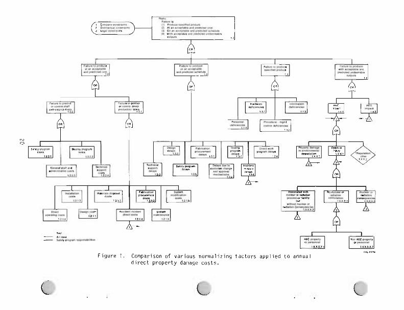
are essentially "safety" in nature (personnel, property, or environmental

harm). These safety areas are those portions of the tree that are in bold-line.

Two points may be noted:

1. The "Safety Program" is found in three of the four major failure

mode branches. The one branch, "failure to produce a specified

product," could include property damage (accident cost), if

quality control inadvertently broke down and permitted impurities or other imperfections in the final product (degrading its value).

2. The safety program is clearly an integral part of the total risk management program. As such, the safety program risk evaluation

must be communicated to management in the programmatic and eco-

nomic language of the project so that it can be combined with or

considered in the same terms as other business risks. While only

one branch is labeled, "Failure to produce at an acceptable and

predictable cost," cost can be assigned to the other branches.

Thus, the "cost" branch is labeled direct costs while the other three branches may be considered as indirect and/or intangible costs.

The tree can be considered in two ways; as a success tree, a failure, or a risk tree.

1. To convert to a risk failure mode tree to a suggestion tree,

change all "or" gates to "and" gates and remove the word failure

from each box. Thus, the total cost of the project is the sum of

the direct support and production costs and the indirect costs of the other three branches. As is clearly illustrated, accident

costs are an integral part of the costs to produce a product.

The transfer symbol indicates that property damage, environmental

harm, death, and injury are considered as direct production

costs, the costs of undesirable outputs, or the cost of delays.

If only direct accident costs are included in direct costs

(Block 1.2.1.81, and the indirect accident costs only are

included under delays (1.3.6) and impact (1.4.1), there will be

no duplication. If, however, as is usually the case for the risk analyst who is considering only accidents, the total costs of

accidents are assessed as a unit for the various hazards (vehicle, inplant property, and personnel), then care must be

taken to avoid duplication of risk.

The tree was not originally intended as a tool or format for

compiling or tabulating risks, but rather as an illustration that to achieve success, management must identify and control the

potential sources of failure. If labor costs, delivery

schedules, quality control, etc., are not controlled, failure will result. A balance must be achieved between control costs and failure probabilities (or risk) to provide an optimum for

success. Either excessive safety program costs or excessive accident costs can jeopardize success.

2. To complete the illustration, consider the tree as a failure tree, as drawn in Figure 1. The failure to control production or accident costs will produce a cost overrun. The risk for each

element in the tree is the probability of control failure

multiplied by the consequence. Evaluating the total tree then

Provides the probable total cost overrun (this is an exercise for

an experienced fault tree analyst). This exercise is not

necessarily recommended, but if assessments are based on most

probable production, delay, product deficiency, and undesirable

output costs, then the cost evaluated from the "success tree"

will be the most probable cost.

Thus, probable accident costs as well as safety program costs must be

included in project cost estimates if the risk of cost overruns and the risk

of project failure are minimized. This concept of risk refers to business

risk and deals with uncertainty of loss estimates. "Risk" as used elsewhere

throughout this document does not include the nonaccident elements of busi-

ness risk. It does include both the loss estimates and the uncertainty in

t h e es t ima tes i n v o l v i n g i n j u r y , exposure t o harmful agents ( h e a l t h e f f ec t s ) ,

p r o p e r t y damage, programmatic delays, and adverse environmental and p u b l i c

impact. The ma jo r s teps r e q u i r e d t o c o n t r o l these losses d e f i n e t h e bas i c

r i s k management progress as f o l l o w s :

1. E s t a b l i s h a company p o l i c y and s e t t o l e r a b l e o r acceptab le r i s k

l e v e l s ; i.e., se t an upper l i m i t o f r i s k beyond which people o r

p r o p e r t y w i l l n o t be exposed; and s e t goa ls f o r m i n i m i z i n g r i s k

2. Determine r i s k and a l l o c a t e resources

3. A l l o c a t e resources

4. Accept reduced r i s k s o r app l y a d d i t i o n a l c o n t r o l s t o f u r t h e r

reduce r i s k

5. M o n i t o r o p e r a t i o n and l o s s c o n t r o l program f o r change.

Since t h e conduct, c o n t r o l , and sa fe t y o f ope ra t i ons a re l i n e f unc -

t i o n s , t h e r e s p o n s i b i l i t y f o r r i s k management r e s t s w i t h l i n e management.

Genera l ly , Steps 2 and 4 ( t h e hazards search and r i s k ana lys is , and t h e

m o n i t o r i n g ) w i l l be de legated t o a sa fe t y o r g a n i z a t i o n because t h e y a re n o t

d i r e c t l y r e l a t e d t o conduct of ope ra t i ons and r e q u i r e s p e c i a l expe r t i se .

Steps 1 th rough 3 ( t h e s p e c i f i c a t i o n , and t h e acceptance of r i s k and a p p l i -

c a t i o n o f c o n t r o l s ) r e q u i r e i n p u t f rom va r i ous groups bo th w i t h i n and o u t -

s i d e t h e company o rgan i za t i on . Regardless o f t h e company o rgan i za t i on , i t

i s impor tan t t h a t each o f t h e f u n c t i o n s be de f i ned and assigned t o a

s p e c i f i c department.

Each of t h e f i v e s teps a re d iscussed below.

1. E s t a b l i s h Acceptable R i sk Leve ls and Goals- -Wi th in t h e c o n s t r a i n t s

of codes, standards, and regu la t i ons , t h e r e i s some l a t i t u d e f o r

t h e manager t o e s t a b l i s h upper l i m i t s o f r i s k . Also, t h e r i s k

management process w i l l i d e n t i f y e i t h e r over o r under r e g u l a t i o n

o f hazards. I n add i t i on , t h e w ise manager o r sa fe t y p ro fess iona l

will not assume that compliance with codes, standards, and regu-

lations is equivalent to adequate safety. Hazards must be sys- tematically identified because no code or standard can ever apply

to all conditions at all times.

The first and primary guide for establishing an acceptable risk

level is that risk not be out of line with that which is commonly

accepted. A second guide is that occupational risk should be

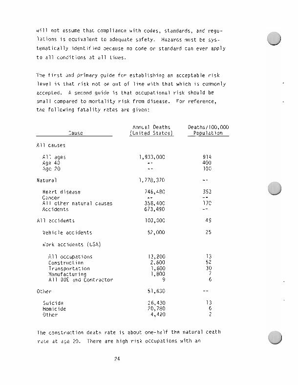
small compared to mortality risk from disease. For reference, the following fatality rates are given:

Annual Deaths Cause (United Statesl

All causes

All ages Aye 40 Age 20

Natural 1,778,370

All accidents 103,000

Vehicle accidents 52,000

Work accidents (USA)

All occupations 13,200 Construction 2,600 Transportation 1,600 Manufacturing 1,800 All DOE and Contractor 9

Other 51,630

Suicide Homicide Other

Deaths/100,000 Population

914 400 100

--

353 -- 170 -- 49

25

13 52 30 7 6

- -

13 6 2

The construction death rate is about one-half the natural death

rate at aye 20. There are high risk occupations with an

Occupational death rate of several hundred deaths per year per

100,000 workers (or approaching the natural death rate at

age 40). The ethics of permitting unequal death rates in

different occupations and the impracticality of equalizing risks

are outside the scope of this document. Our goal is ordinarily

to minimize loss, but not at the expense of subjecting

(sacrificing) any individual to extremely high risks.

One approach that has been suggested for establishing risk

acceptance criteria is that, for involuntary risks to the public,

the death rates should not exceed those from natural causes. As

a guide the following fatality rates per 100,000 population are

siven.

Annual Deaths Deaths/100,000 Cause (United States) Population

All natural causes 1500 Excessive cold 634 Tornado, flood, earthquake 200 Lightning 100

The death rates for both public and occupational rates are

presented only as information. These rates could be used as a

suggested starting point for discussion and establishment of

upper or acceptable levels of risks. The intent of establishing

upper levels is that whatever resources are required to meet these goals should be expended. In any case, total losses should

be small compared to net gain or profit expected from an activity.

In addition to establishing upper risk levels, goals should be

established and plans formulated in order to minimize risk or

cost of accidents.

The total accident cost is the cost of accidents plus the cost of

preventing accidents. These total costs are minimized if large

resources are not expended on small risks or inadequate resources are not allocated to large risks.

Also, goals can be humanitarian; that is, resources could be expended somewhat beyond that which returns economic dividends.

The intangible benefits in improved employee morale and goodwill

may justify a safety program beyond that which can be justified

by tangible losses from accidents. While general goals may be established at the beginning of a project, they may be modified

later if it becomes evident that some goals might be too difficult

or if further gains might be realized.

Finally, several large corporations have outstanding safety pro- grams that demonstrate that extremely low injury rates and prop-

erty loss risk are compatible with efficiency and profitability.

2 . Determine Risk--Since most of this guide deals with hazard identi- fication and risk analyses, only general principles are discussed

in this section. The following steps are applicable to any risk

assessment.

a. Decide what questions need answering and exactly what the risk assessment is to accomplish. Do not obscure the

analysis with irrelevancies.

b. Define the operation being analyzed. Unless the operation

or hazard is bounded and properly documented, the analysis

becomes infinite. The operation being analyzed may be as

simple as a single critical crane lift or as complex as the

entire life cycle of a major operation.

c. Identify hazards. A large number of techniques for identify- ing hazards exist in the literature. All involve classifying

or placing hazards in various categories and systematically

searching each class. A thorough and exhausting search can

be made by using the Risk Identification Tree given in

Appendix A. This method is too detailed and time consuming

to apply to every hazard in a large operation or company. 0

To simplify, the usual hazards from normal industrial acti-

vities can be treated collectively and quantified using

previous accident experience.

d. Assess risk. Determine the potential consequence of each

hazard and the probability of its occurrence. The usual risks of occupational injury, fire, property damage, and

vehicle accident can be treated collectively and quantified using previous accident experience. Unusual or high consequence, low frequency events which cannot be quantified from statistical accident data should be determined

individually and added to the satistical risk. Formulas,

techniques, and methods for assessing the statistical risk

estimates and assessing individual risks are given in the

Analytical Methods section. Multiplying the probability of

each potential loss by its consequence value will give the

risk in units of expected loss. Thus, the units of risk are

the number of fatalities, injuries, workdays lost, quantity of pollution released as well as dollar losses from property

damage, medical expenses, etc. These various types of risk

can be itemized, but to reach a single risk value requires

risk evaluation.

e. Evaluate risk. Evaluating risk requires placing a degree of

undesirability upon the various types of risk. If

equivalencies between environment, safety, and health risk

are established with management concurrence and used in all risk evaluations, much time could be saved; and environment,

safety, and health issues can be treated consistently and

objectively by arguing their relative merits in each proposal. In special situations, the equivalencies could be

reexamined without necessarily compromising this system.

3. Allocate Resources--It is essential to allocate sufficient

resources to a safety program and to line management to control

risks within the upper limits established in Step 1. Additional

resources t o meet goa ls es tab l i shed f o r m in im iz ing r i s k can a l s o

be considered. One c o n s i d e r a t i o n i s t h e c o s t savings i n r i s k

r e d u c t i o n ga ined from a d d i t i o n a l s a f e t y expend i tu res . C

4. Accept Res idua l Risk--The manager r a t h e r t h a n t h e r i s k a n a l y s t

shou ld make t h e f i n a l d e c i s i o n t o accept t h e r e s i d u a l r i s k . How-

ever, t h e a n a l y s t shou ld n o t submit a r i s k r e p o r t t o management

u n t i l he i s s a t i s f i e d t h a t a l l s p e c i a l o r un ique hazards have been

i d e n t i f i e d and adequate c o n t r o l s t o min imize c o s t and ensure t h a t

t h e success o f t h e p r o j e c t o r a c t i v i t y w i l l n o t be j eopa rd i zed by

acc iden ts .

I t i s impor tan t t h a t r i s k r e s p o n s i b i l i t y be c a r e f u l l y de f i ned and

f o r m a l l y documented. As a genera l r u l e , t h e same a u t h o r i t y wh ich

s e t s standards and approves procedures may a l s o bypass sa fe t y

requ i rements . As an example, a foreman was asked i f , i n o rde r t o

meet a schedule, he had a u t h o r i t y t o bypass a l i m i t sw i t ch . H i s

r e p l y was "Yes," b u t when i t was p o i n t e d o u t t h a t l i m i t swi tches

were r e q u i r e d by t h e s a f e t y manual which had been issued under

t h e s igna tu re of t h e General Manager, t h e foreman changed h i s C

mind. I n sho r t , r i s k acceptance procedures a re needed so t h a t

each foreman, superv isor , and employee c l e a r l y understands what

l e v e l of r i s k he i s au tho r i zed t o accept.

5. M o n i t o r i n q and Con t ro l Review of each phase o f a p r o j e c t w i l l

h e l p ensure t h a t t h e e n t i r e l i f e c y c l e i s c a r r i e d o u t i n accord-

ance w i t h t h e c o n t r o l s and l i m i t a t i o n s s e t f o r t h . The o p e r a t i o n a l

c o n t r o l s and t h e r e q u i r e d resources necessary t o m a i n t a i n r i s k s

w i t h i n t h e e s t a b l i s h e d l e v e l s and t o meet t h e minimum r i s k goa l s

w i l l have been i d e n t i f i e d . I n Steps a, b, and c, h i g h l i g h t i n g 6 these c o n t r o l s i n a sa fe t y document f o r d i s t r i b u t i o n t o appro-

p r i a t e design, cons t ruc t i on , i n s t a l l a t i o n , t e s t , opera t ion , main-

tenance, p r o j e c t , q u a l i t y assurance, and s a f e t y groups w i l l

f a c i l i t a t e compl iance.

M o n i t o r i n g w i l l p r o v i d e assurance t h a t t hese c o n t r o l s a re imple-

mented and main ta ined. To be most e f f e c t i v e , t h e m o n i t o r i n g w i l l

beg in a t t h e conceptua l des ign stage and f o l l o w through t o opera-

t i o n and d i s m a n t l i n g and/or decommissioning. (See Opera t i ona l

Readiness-SSDC-1). 7

Design review, q u a l i t y c o n t r o l , and sa fe t y i nspec t i ons w i l l h e l p

assure t h a t no changes a re made which would v i o l a t e t h e sa fe t y

documentat ion w i t h o u t p r i o r rev iew and approva l by those who

reviewed and approved t h e o r i g i n a l s a f e t y documentation. T h i s

m o n i t o r i n g i s a backup t o t h e l i n e manager who has f i r s t and

pr ime r e s p o n s i b i l i t y f o r o p e r a t i n g w i t h i n t h e s a f e t y envelope.

5. REPORT TO MANAGEMENT

The scope and depth of a risk assessment report depends upon the reason

or purpose for doing the assessment. There are at least three separate purposes (types of risk assessments) each of which determine not only the

scope of the assessment but also the content of information reported to

management:

1. Safety Assurance--The first purpose is to assure management that

a specific hazard presents no undue risk to a project or opera-

tion. Risks associated with normal or routine operations may be

acceptable on the basis that qualified safety professionals have

a good safety program. An unusual hazard may surface requiring a

risk assessment. For example at one DOE site, the safety director

became concerned about a proposed location of an office building near the end of an airport runway. To assure management the risk was acceptable, an assessment was made. Only one hazard was con- sidered; that of an aircraft crash into the office building.

Alternatives, such as a different site and additional measures to

reduce risk, were not considered because the probability of a

crash was assessed as very unlikely. Of course had the risk been

unacceptable, the assessment would have been expanded to the

second type discussed below. This risk assessment is included as

an example in Appendix E.

2. CostIBenefit Trade-Offs--This type of assessment evaluates the cost of risk reduction measures against the estimated reduction

in risk. it answers the questions: Are further controls war-

ranted? Which controls are most cost effective? For example, . .

reactor reflector blocks must be shipped cross-country to a test

reactor. Five pairs of five sections are to be shipped on a

single truck. An accident damaging the blocks would delay reactor

startup by one year. Shipping single pairs of dissimilar blocks

on five separate trucks would reduce the probability of reactor

shutdown because it would take two accidents rather than one to shut down the reactor. What is the risk associated with one

t r u c k versus f i v e t r u c k s ? I s t h e e x t r a c o s t j u s t i f i e d ? T h i s

r i s k assessment i s a l s o i nc luded as an example i n Appendix E.

3. Overview R i s k Assessment--This t y p e o f assessment q u a n t i f i e s r i s k s

by hazard ca tego r i es . I t s purpose i s t o assess t h e t o t a l o rgan i -

z a t i o n o r i n d u s t r i a l r i s k and p l a c e these r i s k s i n pe rspec t i ve .

T h i s i n f o r m a t i o n can be used by sa fe t y program d i r e c t o r s and l i n e

managers t o determine if sa fe t y i s balanced, and t o a d j u s t

resource a l l o c a t i o n s o r r e g u l a t i o n s t o achieve a more c o s t e f f ec -

t i v e sa fe t y program. I n t h i s t ype of assessment a l l r i s k s a re

q u a n t i f i e d . Rou t i ne i n d u s t r i a l s a f e t y r i s k s a r e q u a n t i f i e d and

p laced i n pe rspec t i ve t o unusual r i s k s such as nuc lea r o r t o x i c

m a t e r i a l r i s k s . The r i s k r e d u c t i o n e f f ec t s of a d d i t i o n a l resource

t o a p a r t i c u l a r area o f r i s k may be es t imated.

The r i s k r e p o r t w i l l be b e t t e r rece i ved if i t i s c l e a r and communicates

r e s u l t s t o management i n terms of economic cos t and programmatic impact.

Whi le adverse env i ronmenta l and p u b l i c h e a l t h e f f ec t s a re impor tant , t h e

programmatic impact from p u b l i c r e a c t i o n o r r e g u l a t o r y a c t i o n o f these

e f f e c t s shou ld be communicated, if a reasonable es t ima te o f such e f f e c t s

can be made.

Whi le a s p e c i f i c o u t l i n e i s n o t suggested, t h e f o l l o w i n g elements

shou ld be i nc luded on a r e p o r t t o management.

S t a t e tti? r e s u l t s i n conc i se terms summarizing t h e bas i c assumptions

and method. S t a t e t h e purpose of t h e r i s k assessment and why i t i s needed.

The scope of t h e r i s k assessment shou ld be inc luded. Def ine t h e system

be ing analyzed. Acc idents and adverse consequences have f a r reach ing

e f f e c t s and may adve rse l y a f f ec t o t h e r systems. The assessment w i l l be

endless o r incomple te un less l i m i t e d t o a w e l l de f ined system.

Descr ibe t h e method and a n a l y t i c a l model. Discuss t h e l i m i t a t i o n s i f

p o s s i b l e o r g i v e an upper and lower range o f r i s k . A l l t h e c a l c u l a t i o n s

Should n o t be i nc luded i n t h e r e p o r t . The equat ions should be g i ven w i t h

s u f f i c i e n t da ta (on a re fe rence t o da ta ) t h a t t h e a n a l y s i s cou ld be repeated

by a reader. A clear distinction should be made between assumptions or estimates and hard data. If a reader disagrees with any assumption or estimate, it should be easy to insert different assumptions or estimates to

determine the effect on the results. Clearly separate the probability and consequence factors so that different assumptions or estimates of either can easily be inserted into the analysis to test the effect on the risk assessment. Either provide confidence levels on upper and lower bounds with a best estimate.

Discuss factors which were not considered in the analyses because data

were unavailable or for other reasons.

Place detail and data in an appendix in order to keep the body of the

report concise and clear. Basic methods, assumptions, and results should

be readily available to the manager without sorting through a mass of

detail.

If the risk assessment is a costlbenefit trade-off study, those who

bear the cost and the recipients of the benefits should be identified.

Much of the argument generated by many risk reports arise from the fact

that frequently those who reap the benefits are not the ones placed at risk.

Present the results in graphical or tabular form if feasible. Head-

ings, labeling of axis, etc., should be self-explanatory. Too much data on

a single graph will not be as easy to read as several graphs.

If practical, give both the probability of loss and the consequence

with the resulting risk. A catastrophic loss with a low probability may be more important than an equivalent risk with a higher probability and lower

consequence.

The report to management should clearly identify those factors having

the greatest effect on risk, the risk should be clear and well defined with

limitations spelled out and should be communciated in business language

avoiding risk jargon.

6. ANALYTICAL METHODS FOR RISK OUANTIFICATION

Accident risk is the expected or probable loss per unit of time or unit of activity and is equal to the probability of loss multiplied by the mag-

nitude of loss. For any operation, the risk is the sum of the individual risks for each Potential loss.

where

R = risk

C = summation symbol meaning add each consequence multiplied by

its probability

Pi = probability of ith accident

Ci = cost of consequence of ith accident.

Since there is an infinite number of both probabilities and conse-

quences, an accurate quantification of risk requires consideration of the

entire accident cost-frequency spectrum.

6.1 Actuarial Risk Assessment

An actuary is a person who computes insurance premiums or risks based

on statistical data. Thus, actuarial risk assessments are based on accident

experience. Data can be obtained from Accident ~ a c t s ~ published by the

National Safety Council, an Almanac, the U.S. Statistical Abstract, the

Bureau of Labor Statistics, or numerous safety records and reports main-

tained either by individual companies or by National/International Agencies

such as the National Transportation Safety Board. The following vehicle risk problem is following as an example of actuarial risk assessment.

6.2 Example Problem

What is the annual risk of driving to and from work for the average

person?

Accident Facts, 1981 edition, Page 40, indicates that in 1980 there 7 were 2.98 x 10 accidents and a total vehicle mileage of 1.511 x 10" miles.

The unit probability is:

7 P = 2.98 x 10 accidents

= 1.97 x accidents/vehicle - miles. 1.511 x 10'' vehicle - mileage

The exposure is the number of miles driven: assuming 20 rniles/day and

225 work-dayslyear gives 4500 miles/year, P annual = the annual

probability is:

5 accidents 4.5 1 . 9 7 ~ 1 0 - mile 3 miles = accidents year-person 0.08' year-person

Accident Facts, 1981 edition, Page 4, indicates a total monetary loss 6 of $39.3 x lo9. With 29.8 x 10 accidents, the average cost is $1319

including wage loss, medical expense, insurance, and administrative costs

as well as repair costs. Indirect losses associated with legal courts and cargo damage are not included.

Risk = probability x average cost

accidents 1319 dollars Risk = 0.089 year accident = $117.39/year

Risk = 0.089 x 1319 = $117.39/year.

To calculate the risks of each consequence separately, multiply the

costs for wages lost, medical expense, insurance administration, and

property damage as given on Page 5 of Accident Facts by the probability,

0.089.

The fatality risk can be similarly calculated:

Accident Facts, Page 40, gives 52,600 deaths in 1980. The mileage given previously is 1.511 x 1012. The probability, P, is:

The exposure (mileage) is the same, 4500 mileslyear. Thus the annual fatality probability for an individual, Pf is:

miles -8 deaths = x 3.48 x 10 -mx deaths 'f = 4500 year-person year-person .

The probability becomes more meaningful if we convert the probability

of death to expected days lost assuming an average of 35 years lost for

each death.

Risk = 1.6 , deaths , Gsrs 365 days = 2.04 days. year 2 death year

Thus, on an average, there are four days of human life lost for each person

driving to and from work for one year.

The risk can also be stated in economic terms assuming $600,000 for

the value of a life, the risk is $600,000 x 1.6 x or $96/year. In terms of productivity loss, the risk is one-half if we assume a lifetime

salary of $600,000 ($20,00O/year for 30 years):

2.04days lostlyear ~20,000~year 30 year 365 dayslyear 70 years in lifetime = $48/year.

Note that the 4.1 days lost/year is divided by 365 days because the

days of life lost are not necessarily work days.

0 Conditional probability is the probability of a consequence conditioned on the probability of a prerequisite event. For example, the calculated

annual probability of an accident in the above example was 0.089lyear. The conditional probability of a fatality is the probability of fatality if an

accident occurs and is the number of fatalities divided by the number of

accidents. With 52,600 deaths and 29,800,000 accidents, this probability

is 52,600 divided by 29,800,000 or 0.001765 fatalitieslaccident which is

one fatality for each 56.65 accidents.

TO find the probability of a fatality from the conditional probabil-

ity, multiply the first event (the accident) by the conditional probabil-

ity of a fatality should the accident occur: 0.089 accidentslyear x 0.00176 fatalitylaccidents = 1.6 x 10-~/year, the same value as

calculated directly.

6.3 Subjective Risk Estimate

The following example illustrates a process by which a subjective estimate of the annual probability of an accident fatality can be made if

data are not available. 0 In a community of 30,000 to 40,000, one reads about a fatality several

times each year. The number of fatalities is certainly not 501year and its

surely more than llyear. A value between these extremes will provide the best estimate. The arithmetic average is (50 + I) divided by 2 or 25.5. However, this value is a factor of 2 below the maximum value but is a factor

of 25 greater than the minimum value. The geometric average will be an

equal factor above and below the minimum and maximum values and will have

the least chance of large error (a large factor above or below the actual

value). To obtain the geometric average, the logarithm of the maximum and

minimum are averaged and converted back to the geometric average:

In = 50 = 3.91

In 1 = 0

In 50 + In 1 = 3.91

112 (In 50 + In 1) = 1.96 antaloq of 1.96 = 7.07.

Th is va lue o f 7 dea ths l yea r i n 117 t h e maximum and 7 t imes t h e minimum i s

l i k e l y t o be w i t h i n a f a c t o r of 2 o r 3 o f t h e a c t u a l va lue.

More than h a l f of t h e acc iden ts seem t o occur evenings o r weekends, so

we es t ima te two f o r d r i v i ng - to -work f a t a l i t i e s . We es t ima te 1/4 of t h e c i t y

p o p u l a t i o n (10,000) dr ive- to-work . Two f a t a l i t i e s ou t of 10,000 workers 4 equa ls a p r o b a b i l i t y of 2 x 10- l yea r , i n good agreement t o t h e s t a t i s t i -

4 c a l va lue of 1.6 x 10- /year. A s i m i l a r p rocess of l o o k i n g a t each p i e c e

of a problem w i l l y i e l d es t ima tes of r i s k which a re p re fe rab le t o pu re

guesses o r hunches when l o g i c a l dec i s i ons a re needed. As new in fo rma t i on

becomes a v a i l a b l e t h e s u b j e c t i v e es t ima tes can be modi f ied . A r i g o r o u s

method f o r a d j u s t i n g p r o b a b i l i t i e s g i v i n g we ight t o b o t h t h e s u b j e c t i v e

es t ima te and new in fo rma t i on i s g i ven by Bayes Theorem which i s t r e a t e d i n

most s t a t i s t i c s tex tbooks.

6.4 Survey Methods

F requen t l y , i n fo rma t i on needed f o r a r i s k assessment can be ob ta ined

by us ing an employee ques t i onna i re . For example, d ispensary reco rds f o r an

EKDA c o n t r a c t o r i n d i c a t e t h a t an average of n i n e t o e i n j u r i e s occur red p e r

year. Even though t h e c o n t r a c t o r operated a shoe s t o r e and p e r m i t t e d

employees t o purchase sa fe t y shoes a t cos t , many employees chose n o t t o wear

them. To determine t h e wor th of t h e s a f e t y shoe program investment, t h e

r i s k d i f f e r e n t i a l between those who wore sa fe t y shoes and those who d i d n o t

had t o be es tab l i shed . An employee ques t i onna i re was se lec ted as t h e means

f o r o b t a i n i n g t h e r e q u i r e d d a t a and was completed b y about 300 employees.

The a n a l y s i s o f t h e i n p u t s revea led t h e f o l l o w i n g .

About 58% of t h e shopworkers wore sa fe t y shoes w i t h an annual i n j u r y

r a t e o f 0.003 t o e i n j u r i e s pe r shopworker. Shopworkers n o t wear ing s a f e t y

shoes had an i n j u r y r a t e of 0.04. Nonshopworkers n o t wear ing sa fe t y shoes

had 0.003 t o e i n j u r i e s pe r yea r pe r employee, w h i l e no t o e i n j u r i e s were

r e p o r t e d f o r nonshopworkers wear ing s a f e t y shoes, i n d i c a t i n g t h a t t o e i n j u r y

r i s k f o r nonshopworkers was smal l , whether wear ing sa fe t y shoes o r not.

Based on an average va lue o f $150/toe i n j u r y , t h e annual t o e i n j u r y

r i s k f o r each shopworker wear ing s a f e t y shoes i s $0.45, and i s $6.00 f o r

those n o t wear ing safe ty shoes. For t h e company as a whole, t h e t o e i n j u r y

r i s k was es t imated t o be $1500/year. If no employee wore s a f e t y shoes, t h e

company r i s k would be $3000; b u t t h e r i s k would o n l y be $200 if everyone

wore sa fe t y shoes. Management can now weigh t h e c o s t s of a sa fe t y shoe

program aga ins t these r i s k values. Other fac tors , such as OSHA

requirements, w i l l a l s o i n f l uence t h e dec i s i on , b u t w i t h such a survey t h e

manager can ge t a f e e l f o r t h e economic r e t u r n from h i s sa fe ty shoe

investment.

A survey w i l l u s u a l l y r e q u i r e t h e se rv i ces of a research

s t a t i s t i c i a n . Anyone conduct ing a survey shou ld f o l l o w these bas i c r u l e s :

1. I d e n t i f y t h e problem.

2. Survey t h e l i t e r a t u r e .

3. Discuss t h e f e a s i b i l i t y of t h e proposed survey w i t h management.

E x p l a i n t h e p o t e n t i a l b e n e f i t s of t h e survey t o enhance y o u r

chance of o b t a i n i n g management coopera t ion .

0

4. De f i ne i n c l e a r s p e c i f i c terms t h e survey ques t i on (8 ) t o be

answered.

5. Develop t h e ques t i onna i re w i t h an i n s t r u c t i o n sheet. Exp la in t h e

purpose o f t h e quest ionna i re . Keep t h e ques t i ons as s imple as

p o s s i b l e . Put t h e i n s t r u c t i o n s on a separa te sheet r a t h e r t han

on t h e back o f t h e ques t i onna i re .

6. Search c a r e f u l l y f o r ambigu i t ies . Tes t t h e ques t i onna i re on a

few r e p r e s e n t a t i v e i n d i v i d u a l s and r e v i s e as appropr ia te .

7 . Request l i n e management d i s t r i b u t i o n and c o l l e c t i o n of t h e

ques t i onna i re .

8. Evaluate t h e d a t a and draw conc lus ions. 0

38

9. Preparc r e p o r t t o management. E x p l a i n assumptions and methods i n

s u f f i c i e n t d e t a i l t o pe rm i t r a p i d r e e v a l u a t i o n i f assumptions a re

changed.

6.5 Insurance R isk

Cons ider insurance as i t r e l a t e s t o r i s k . A company i n s u r i n g 100 c a r s

f o r p r o p e r t y damage w i l l es t ima te t h e average l o s s p e r yea r as f o l l ows . On

an average, 10 c a r s o u t o f 100 w i l l s u s t a i n p r o p e r t y damage d u r i n g a year .

The average l o s s has been $500. Thus, we can expect t h e l o s s d u r i n g t h e

y e a r t o be $500 x 10 o r $5000. To pay t h e $5000, t h e insurance company must

c o l l e c t t h e $5000 f rom t h e 100 c a r owners o r $50 each. The $50 i s t h e mea-

su re of r i s k f o r each c a r owner. If n o t insured, t h e c a r owner has a l a r g e

(90% chance) of no l o s s and a smal l (10% chance) o f a $500 l o s s ( a $50

r i s k ) . The insurance company accepts t h e r i s k of a l l 100 owners so i t s r i s k

i s t h e sum o f t h e i n d i v i d u a l owner r i s k s o r $5000. The company r i s k w i l l

v a r y l e s s t han t h a t of t h e i n d i v i d u a l . The i n d i v i d u a l has a 90% chance of

no l o s s and 10% chance of a $500 loss . The company has a 10% chance of

Paying o u t $2500 and a 90% chance of pay ing ou t $7500. I n an average yea r

t h e insurance company's payout w i l l equal t h e $5000 taken i n t o cover t h e

r i s k . I n a c t u a l p r a c t i c e , t h e insurance company w i l l r e q u i r e a l a r g e r

premium than $500 ($50 pe r c a r owner) t o cover a d m i n i s t r a t i v e cos ts ,

p r o f i t , e t c .

The va r i ance becomes s m a l l e r as t h e number of acc iden ts becomes l a r g e r .

The standard d e v i a t i o n i s a measure o f t h i s v a r i a t i o n and i s t h e square

r o o t o f t h e number o f acc idents . I n t h e i l l u s t r a t i o n above, t h e number of

acc iden ts each yea r would be 10 + fi o r 10 + 3.2. The 90% l e v e l i s

1.645 f i o r 5, so t h e 10 t o 90% conf idence range i s 5 t o 15 acc iden ts o r

$2500 t o $7500 a t $500/accident. The standard d e v i a t i o n f o r 10,000 cases

i s o n l y 1% of 10,000, compared t o 10% f o r 100 cases and 32% f o r 10 cases.

6.6 L i f e Shor ten ing E f f e c t s

F o r any s p e c i f i c causes o f death, t h e p r o b a b i l i t y o f dy ing can be

r e l a t e d t o t h e average decrease i n l i f e expectancy." For s p e c i f i c

hazards with a small probability of death compared to the natural death

rate, the reduced life expectancy can be estimated by the following method

(automobile accidents are used as an example):

1. Calculate the lifetime probability of death from a vehicle

accident:

In 1981, there were 55,000 vehicle accident deaths of a total 1,900,000 deaths. Since 2.9% (55,000 divided by 1,900,000) of all deaths result from vehicle accidents and each individual is

sure to die, the lifetime probability of a vehicle accident is

0.029.

This estimate can also be calculated as follows:

- 4 55,000 vehicle deathslyears = 2.5 220,000,000 U.S. population

Multiplying the annual probability by 70 years (the average life-

time) gives 0.0175. This value is in reasonable agreement. This

calculation assumes there are an equal number of people in each

age group and an equal probability of vehicle fatality at each

age. Thus, the higher value of 0.025 is more correct. (For most

risk estimates this degree of difference is not large.)

2. Estimate the average years lost by assuming the fatality occurred

midway through life; i.e., multiply the lifetime death probability

by 35 to obtain expected number of years lost:

0.025 x 35 = 0.875 years reduced life expectancy.

For motor vehicles, this estimate of reduced life expectancy would be

somewhat low because younger males have a higher probability of a motor

vehicle facility. A more accurate estimate could be made by calculating reduced life expectancy for specific age groups (male and female sepa-

rately). For most risk assessments, such accuracy is not necessary, and

the data are not usually available.

S t a t i n g f a t a l i t y consequences i n terms of reduced l i f e expectancy,

r a t h e r t han i n terms of l i v e s l o s t , i s more a p p r o p r i a t e f o r hazards such as

smoking o r a i r p o l l u t i o n which k i l l th rough increased cancer o r l ung and

h e a r t disease. These e f f e c t s a re more pronounced i n t h e l a t e r yea rs o f

l i f e , so t h a t t h e number of deaths does n o t g i v e a c l e a r p i c t u r e . Many who

smoke h e a v i l y w i l l d i e e a r l i e r t han i f t h e y d i d n o t smoke. Thus, a pub-

l i s h e d es t ima te o f t h e number o f deaths pe r y e a r from smoking i s n o t mean-

i n g f u l un less t h e b a s i s f o r t h e es t ima te i s a l s o given. For example, were

o n l y deaths caused by d iseases c l o s e l y assoc ia ted w i t h c i g a r e t t e smoking

( l u n g cancer ) counted? Was i t a s t a t i s t i c a l es t ima te of t h e number o f e a r l y

o r Premature deaths based on a s tudy of age of death d i f f e r e n c e s between

smokers and nonsmokers?

If t h e e s t i m a t i o n i s t h e number of e q u i v a l e n t 1 i v e s l o s t based on

70 years pe r l i f e , what was t h e average number of yea rs l o s t pe r e a r l y

death? It i s obv ious l y n o t an average of 35 yea rs (midway th rough l i f e as

assumed f o r a c c i d e n t s ) .

One pe rcen t o f t h e p o p u l a t i o n dy ing 35 years e a r l y and 35% o f t h e

p o p u l a t i o n dy ing 1 y e a r e a r l y i s d i f f e r e n t ; b u t each r e s u l t i n t h e same

e q u i v a l e n t number o f " l i v e s l o s t ' ' o r i n t h e same reduced l i f e expectancy.

There i s no a p r i o r i " c o r r e c t ' way t o measure t h e r i s k o f h e a l t h e f f e c t s o r

l o s s of l i f e . I t i s impor tant , however, t h a t comparisons o f d i f f e r e n t

r i s k s i n v o l v i n g l o s s of l i f e be made on a conse rva t i ve basis, and t h a t t h e

methods and assumptions be s p e c i f i c a l l y s t a t e d i n t h e r i s k assessment.

Departures from t h e norm and any assumptions shou ld be descr ibed

q u a l i t a t i v e l y and, as p r a c t i c a l , q u a n t i t a t i v e l y .

6.7 Trend Ana l ys i s

The measurement of sa fe t y performance i s e s s e n t i a l t o e v a l u a t i o n o f

new techn iques o r methods of reduc ing r i s k , such as proposed i n t h e

preced ing s e c t i o n of t h i s guide. D i scuss ion of a comprehensive s a f e t y

i n fo rma t i on system, which would p r o v i d e good i n d i c a t o r s o f f u t u r e sa fe t y

performance, i s i nc luded i n another SSDC document.19 O f concern here i s

o n l y t h e a n a l y s i s of p r o p e r t y damage and i n j u r y d a t a i n o rde r t o determine

whether a t r e n d o r change i n acc iden t r a t e s i s s t a t i s t i c a l l y s i g n i f i c a n t .

In a period of inflation and/or company growth, total accident costs will also increase unless there is a compensating decrease in accident

rates. Frequency and severity rates are indicators of performance rather

than total loss. Also, cents loss per $100 property valuation is a method of measuring performance. However, factors such as number of employees (employee-hours worked), inflation (dollar value), and vehicle miles can be

applied to loss data in order to determine whether an increase or decrease

in accident costs (or frequency, severity, property loss rates) is

significant or whether it could have happened as a result of random variation.

For example, during 1975, an ERDA (now DOE) contractor experienced

large increases in 1975 over 1974 in-plant property damage, vehicle damage,

and the number of injuries. Were these increases significant, or could

they have happened by chance? From 1971 through 1975, the number of employees (and hence employee-hours) increased by 20%, and the number of vehicle miles increased by 32%. In addition, inflation increased by 35%. In order to determine if there was a significant trend in loss experience,

these data (inflation, employee-hours, and vehicle miles) were determined

and compared for each year, 1971 through 1975.

The number of property damage incidents and the number of injuries

were normalized to employee-hours, while vehicle accidents were normalized

to mileage. The cost per incident of both vehicle and property damage was

normalized to the cost of living index. Public liability and fires were

not analyzed since the experience to date has been so limited that any attempt to predict a trend would be meaningless. The normalized vehicle and property damage costs were obtained by multiplying the normalized cost

per incident by the normalized number of incidents.

The normalizing factors and the normalized accident data are given in

Table 2. As can be seen, all normalized 1975 values are within or close to

one standard deviation. (The number of vehicle incidents is low by 1.1,

but this is not significant because this value would occur one out of four

times by chance.) The overall data show a general random character with no

discernible trend.

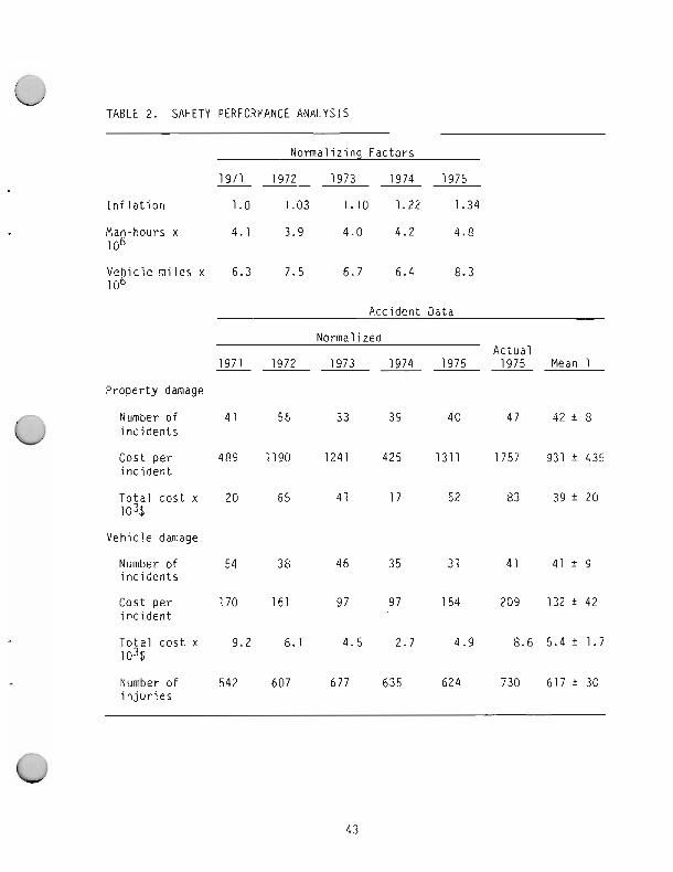
TABLE 2. SAFETY PERFORMANCE ANALYSIS

Normal iz ing Fac to rs

1971 1972 1973 1974 1975 ----- I n f l a t i o n 1.0 1.03 1.10 1.22 1.34

Man-hours x 4.1 3.9 4.0 4.2 4.8 106

Veh i c l e m i l e s x 6.3 7.5 6.7 6.4 8.3 106

Normal ized Ac tua l

1971 1972 1973 1974 1975 1975 Mean1 ------ Proper t y damage

Number o f 4 1 56 33 39 40 47 42 t 8 i n c i d e n t s

Cost p e r 489 1190 1241 425 1311 1757 931 t 435 i n c i d e n t

T o t a l c o s t x 20 65 41 17 52 83 39 i 20 103$

Veh i c le damage

Number o f 54 38 46 35 3 1 41 41 t 9 i n c i d e n t s

Cost p e r 170 161 97 97 154 209 132 i 42 i n c i d e n t

T o t a l c o s t x 9.2 6.1 4.5 2.7 4.9 8.6 5.4 t 1.7 l o3$

Number of 542 607 677 635 624 730 617 t 30 i n j u r i e s

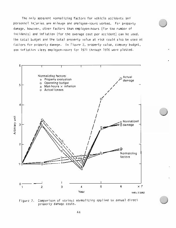
The o n l y apparent no rma l i z i ng f a c t o r s f o r v e h i c l e acc iden ts and

Personnel i n j u r i e s are mi leage and employee-hours worked. For p r o p e r t y

damage, however, o t h e r f a c t o r s t han employee-hours ( f o r t h e number of

i n c i d e n t s ) and i n f l a t i o n ( f o r t h e average c o s t p e r acc iden t ) can be used.

The t o t a l budget and t h e t o t a l p r o p e r t y va lue a t r i s k cou ld a l s o be used as

f a c t o r s f o r p r o p e r t y damage. I n F i g u r e 2, p r o p e r t y value, company budget,

and i n f l a t i o n t imes employee-hours f o r 1971 through 1976 were p l o t t e d .

Normalizing factors: o Property evaluation o ODeratina budaet " o an-hours x inflation 0 Actual losses

Actual , damage

Year INEL23362

F i g u r e 2. Comparison o f va r i ous no rma l i z i ng a p p l i e d t o annual d i r e c t p r o p e r t y damage costs .

These three factors were applied to actual property loss, and the resulting

normalized property damages were also plotted. In addition, all data nor-

malized to a value of one for 1971 to permit direct comparison of the three

factors yield remarkably similar results. (The budget and property value inherently include inflation. Employee-hours, however, must be multiplied

by inflation. The reason for this is employee hours times inflation pro-

vides a constant measure of company property investment for a given plant,

assuming wages are not rising faster or slower than property value.)

The various normalizing factors appear to provide consistent results.

It is concluded that any of the above normalizing factors are acceptable,

and the cents loss per $100 property value is a good performance indicator.

6.8 Loq-Normal Distribution

The simplest, first cut, method of assessing the average cost of an

accident is to divide the total cost of accidents (of particular type) by the number of accidents.

The result, the total cost of last year's accidents, is an estimate of

next year's risk; but only if the very costly or catastrophic accident is

properly represented in the accidents of the previous year. This simple

approach can lead to underestimating the risk. First, all of the conse-

quences may not have been considered or represented in the experience data.

With vehicles, which we are using for an example, the property damage may

be adequately represented but the number of injuries or fatalities are

likely to be few or none with a small data base of vehicle accidents. In

such cases, the average number of fatalities can be estimated from statis-

tical data: the injury and/or death rate per million vehicle miles for all

DOE can be used to calculate the injury per death risk for a specific field

office or contractor. However, due to peculiarities of a particular con-

tractor's operation or climate conditions, such estimates must be made with

caution.

The average cost can similarly be estimated from a larger data base. The average loss per event for a given contractor should be compared to the

average l o s s Per event f o r a l l DOE con t rac to rs . I f t h e d i f f e r e n c e i s s i g - n i f i c a n t , t hen t h e r i s k ana l ys t must determine whether t h e s p e c i f i c con-

t r a c t o r ' s average l o s s Per event i s l i k e l y t o be d i f f e r e n t o r whether t h e

s i n g l e c o n t r a c t o r ' s exper ience i s inadequate t o determine an average. A

qu ick rev iew of t h e da ta may revea l t h e answer. I f a l l o f t h e acc iden ts

have been minor ( f r e q u e n t l y t h e s i t u a t i o n w i t h few acc idents) , t h e long-

te rm average acc iden t c o s t i s l i k e l y t o be h ighe r t h a n t h e c o s t based on

recen t pas t exper ience. A q u i t e u n l i k e l y , b u t poss ib le , oppos i t e s i t u a t i o n

i s t h a t o n l y one acc ident occur red b u t t h e c a r was " t o t a l e d . " The long-

t e rm average acc iden t c o s t w i l l be l ess . The second problem c l o s e l y r e l a t e d

t o t h e f i r s t i s t h a t t h e f r equency -seve r i t y r e l a t i o n s h i p s of t h e same t y p e

of acc iden t may v a r y cons ide rab l y from one c o n t r a c t o r t o another. That i s ,

t h e p r o b a b i l i t y of death based on t h e number of i n j u r i e s may v a r y g r e a t l y .

I t i s c e r t a i n l y n o t t h e same f o r a h i g h r i s e s t e e l worker and an o f f i c e

worker. The p r o b a b i l i t y of a c a t a s t r o p h i c f i r e may n o t be d i r e c t l y p ropo r -

t i o n a l t o t h e number of waste basket f i r e s . Fac to rs such as t ypes of con-

s t r u c t i o n , absence of s p r i n k l e r systems, etc., may have a g r e a t e r bea r i ng

on t h e p r o b a b i l i t y of a ma jo r f i r e and how i t w i l l a f f e c t t h e average c o s t

o f f i r e s .

Assessing r i s k us ing t h e average c o s t of p a s t acc iden ts w i l l u s u a l l y

r e s u l t i n a gross unde res t ima t i on o f r i s k . Acc ident p a t t e r n s a re random

events w i t h a log-normal o r skewed d i s t r i b u t i o n . F o r a l i nea r -no rma l

d i s t r i b u t i o n , t h e average c o s t o f an event i s a l s o t h e c o s t which occurs

most f r equen t l y . F o r acc idents , t h e average c o s t i s u s u a l l y l a r g e r t han

t h e most f r e q u e n t l y o c c u r r i n g cos t . Th i s i s because t h e ve ry l a r g e o r

c a t a s t r o p h i c acc iden t may (and f r e q u e n t l y does) c o n s t i t u t e a s i g n i f i c a n t

p o r t i o n o f t h e r i s k event though none have occur red r e c e n t l y .

A n a l y s i s of t h e f r equency -seve r i t y p a t t e r n s of p rev ious acc iden ts us ing

va r i ous t ypes of p r o b a b i l i t y graph paper can p r e d i c t t h e p r o b a b i l i t y of

l a r g e acc idents , de termine t h e average c o s t of acc idents , and p r o v i d e a

b e t t e r r i s k p i c t u r e .

The log-normal graph paper has a p r o b a b i l i t y sca le which conve r t s t h e

p r o b a b i l i t y curve t o a s t r a i g h t l i n e . The consequence ( c o s t ) sca le i s

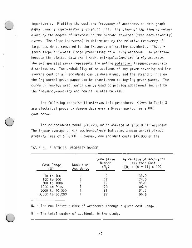
logarithmic. Plotting the cost and frequency of accidents on this graph Paper usually approximates a straight line. The slopp of the line is deter-

mined by the degree of skewness in the probability-cost (frequency-severity)

curve. The slope (skewness) is determined by the relative frequency of

large accidents compared to the frequency of smaller accidents. Thus, a st@& slope indicates a high probability of a large accident. In addition because the plotted data are linear, extrapolations are fairly accurate.

The extrapolated curve represents the entire potential frequency-severity

distribution. The probability of an accident of any given severity and the average cost of all accidents can be determined, and the straight line on

the log-normal graph paper can be transferred to log-log graph paper. The curve on log-log graph which can be used to provide additional insight to

the frequency-severity and how it relates to risk.

The following exercise illustrates this procedure: Given in Table 3

are electrical property damage data over a 5-year period for a DOE

contractor.

The 22 accidents total $66,220, or an average of $3,010 per accident.

The 5-year average of 4.4 accidentslyear indicates a mean annual direct

property loss of $13,200. However, one accident costs 149,000 of the

TABLE 3. ELECTRICAL PROPERTY DAMAGE

Cumulative Percentage of Accidents Cost Range Number of Less than Cost

(6) Accidents mi) {[Ni + ( N + I)] x 1001

Ni = The cumulative number of accidents through a given cost range.

N = The total number of accidents in the study.

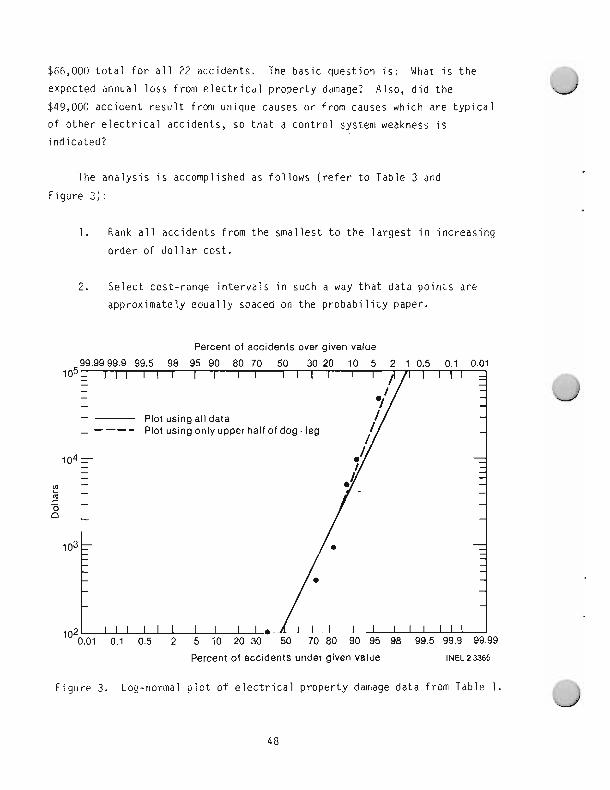
$66,000 total for all 22 accidents. The basic question is: What is the expected annual loss from electrical property damage? Also, did the

$49,000 accident result from unique causes or from causes which are typical

of other electrical accidents, so that a control system weakness is

indicated?

The analysis is accomplished as follows (refer to Table 3 and

Figure 3):

1. Rank all accidents from the smallest to the largest in increasing

order of dollar cost.

2. Select cost-range intervals in such a way that data points are

approximately equally spaced on the probability paper.

Percent of accidents over aiven value

Percent of accidents under given value 1 ~ ~ ~ 2 3 3 6 5

Figure 3. Log-normal plot of electrical property damage data from Table 1. (J

3. List the number of accidents for each cost range, as well as the

cumulative number of accidents to that point.

4. Calculate the cumulative percentage for each cost range (as in

Table 3) and plot the cost versus the cumulative percentage on

log-normal paper (as in Figure 3). The cumulative percentage is

calculated by dividing the cumulative number (Ni) ineach cost

range by the total number of events plus one, and multiplying the result by 100. (We divide by N + 1 because "Nu points divide a line into N + 1 segments.)

The following guides explain how to interpret the resulting curve.

1. If the accident is an outlier, the accident is probably unique,

and change analysisl0 to determine the need for a specific fix

for the unique accident is indicated. On the other hand, if the

slope is steep (high probability of a large accident and the

$49,000 accident fits the rest of the data, as in this example)

the $49,000 is typical of the system. If the indicated frequency

is unacceptable, systems analysis is required to prevent reoccurrence.

2. If the slope increases with cost (curves upward), the system may

be diverging out of control. Careful attention to cause of

increase is critical.

3. If the plotted line approximates a dog-leg with the two segments

fairly straight, two different basic causes are probably involved. For example, the curve for small fires which are extinguished may not have the same slope as the curve for large fires beyond the

control of fire fighting capabilities. Another example is that

planned radiation exposures should not have the same character- istics as unplanned large exposures.

4. If the plotted line flattens out at the top (smaller slope), there

may be a limit to the consequence. For example, the maximum

damage t o a v e h i c l e equa ls t h e va lue of t h e veh i c l e , and thus t h e

s i n g l e v e h i c l e acc ident d a t a w i l l approach t h i s va lue asympto t i -

c a l l y as l ong as we cons ide r o n l y v e h i c l e p r o p e r t y damage.

5. If t h e p l o t t e d l i n e f l a t t e n s a t t h e bottom, t h e r e i s p robab l y a

r e p o r t i n g o r n a t u r a l minimum. For example, a cu rve of a l l

acc iden ts g r e a t e r t han $50,000, as r e p o r t e d by DOE c o n t r a c t o r s ,

f l a t t e n s ou t and approaches t h e $50,000 consequence l e v e l

asymp to t i ca l l y . Thus, i n t h e $50,000 t o $100,000 acc iden t range,

t h e f r equency -seve r i t y s l ope i s d i s t o r t e d .

6. The frequency of occurrence ( o r r e t u r n p e r i o d i n extreme va lue

,language) f o r any g i ven s i z e acc iden t can be ca l cu la ted . For

example, i n F i g u r e 3 about 1.3% o f e l e c t r i c a l acc iden ts w i l l c o s t

more t h a n $100,000. S ince 4.4 acc iden ts have occur red each year,

a g r e a t e r t han $100,000 acc ident i s expected about once eve ry 17

o r 18 years [1/(0.013 x 4.4)]. Note t h a t t h e d a t a p o i n t s

( c i r c l e s ) i n F i g u r e 3 e x h i b i t a s l i g h t dog- leg c h a r a c t e r i s t i c .

If a s t r a i g h t l i n e i s f i t t e d t o t h e upper h a l f o f t h e data, t h e

p r o b a b i l i t y of a g r e a t e r t han $100,000 acc iden t increases t o

2.3%. w i t h a r e s u l t i n g expected f requency of eve ry 7.5 t o

11 years. [As w i l l be seen i n t h e example f o r extreme va lue

a n a l y s i s (d iscussed i n t h e n e x t sec t i on ) , which uses o n l y t h e

maximum acc ident i n each of t h e 5 years, t h e extreme va lue

a n a l y s i s p r e d i c t s a r e t u r n p e r i o d o f 10 years. Thus, t h e upper

h a l f l i n e i s p robab l y more accurate. However, one should n o t be

concerned w i t h t h i s d i f f e r e n c e ; t h e r e t u r n p e r i o d s a re w i t h i n a

f a c t a r o f 2, wh ich i n d i c a t e s good agreement f o r t h e l i m i t e d

amount o f data. ]

A d d i t i o n a l i n f o r m a t i o n f rom t h e d a t a can be ob ta ined by t r a n s f e r r i n g

t h e log-normal cu rve ( F i g u r e 3) t o l og - l og paper (F igu re 4 ) . I n making t h e

t r a n s f e r , use t h e "percent ove r " sca le above F i g u r e 3. S e l e c t t h e p o i n t s

t o t r a n s f e r f rom t h e curve, n o t t h e c i r c l e d d a t a p o i n t s . F o r example, t h e

f i r s t (x, y ) p o i n t t o t r a n s f e r , (51%, $100) on F i g u r e 3 becomes 0.4'3 on t h e

y a x i s and $100 on t h e x -ax is . The second p o i n t on F i g u r e 3 ( x = 20%) y =

$1000 becomes 0.20 on y - a x i s and $1000 on t h e x -ax i s i n F i g u r e 3.

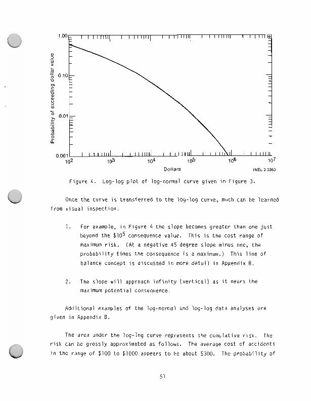
Dollars INEL 2 3353

F i g u r e 4. Log- log p l o t o f log-normal curve g i v e n i n F i g u r e 3.

Once t h e cu rve i s t r a n s f e r r e d t o t h e l o g - l o g curve, much can be l ea rned

f rom v i s u a l i nspec t i on .

1. For example, i n F i g u r e 4 t h e s lope becomes g r e a t e r t han one j u s t

beyond t h e $ l o 5 consequence value. T h i s i s t h e c o s t range o f

maximum r i s k . ( A t a nega t i ve 45 degree s lope minus one, t h e

p r o b a b i l i t y t imes t h e consequence i s a maximum.) Th i s l i n e of

ba lance concept i s d iscussed i n more d e t a i l i n Appendix B.

2. The s lope w i l l approach i n f i n i t y ( v e r t i c a l ) as i t nears t h e

maximum p o t e n t i a l consequence.

A d d i t i o n a l examples o f t h e log-normal and l o g - l o g d a t a analyses a r e

g i v e n i n Appendix B.

The area under t h e l o g - l o g cu rve rep resen ts t h e cumula t ive r i s k . The r i s k can be g r o s s l y approximated as f o l l o w s . The average cos t of acc iden ts

i n t h e range of $100 t o $1000 appears t o be about $300. The p r o b a b i l i t y of

an accident in this cost range (taken from t h e curve in Figure 4) given an

accident is about 0.6 - 0.25 or 0.35. The risk is the consequence times the

probability or about $105. Repeating this process for each cost range and

summing gives the average cost of an accident. This average is more accu-

rate than the total cost of accidents divided by the number of accidents,

because it gives proportionate representation to the large accident which

occurs too infrequently to be accurately represented in experience data.

A more accurate estimate can be obtained by integrating the curve as follows (refer back to Figure 3).

1. Approximate the curve with a series of straight lines. In this

case, a straight line for each decade introduces only a small

error.

2. Integrate each line separately and sum the results. The general

equation of a straight line on log-log paper is:

where

C = cost of the accident

f = frequency or probability of the accident

A = the slope of the line which is a constant for a

straight line.

NOTE: For any type of accident, for a given cost, there is a

different probability of occurrence. Generally, as the cost

increases, the probability decreases. We can choose to integrate

over frequency or cost, depending on whether we wish to know the

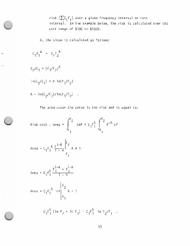
risk (Ccifi) over a given frequency interval or cost

interval. In the example below, t h e risk is calculated over the

cost range of $100 to $1000.

A, the slope is calculated as follows:

C2/Cl = (fl/f2) A

ln(C2/Cl) = A ln(fl/f2)

A = ln(C2/Cl)/ln(fl/f2) .

The area under the curve is the risk and is equal to:

fl-A - fl-A A I Area = Clfl _ A 2

1-A Area = ClflA

A = Clfl (In f2 - In fl) = Clf? In f2/fl

f2 A # 1

1

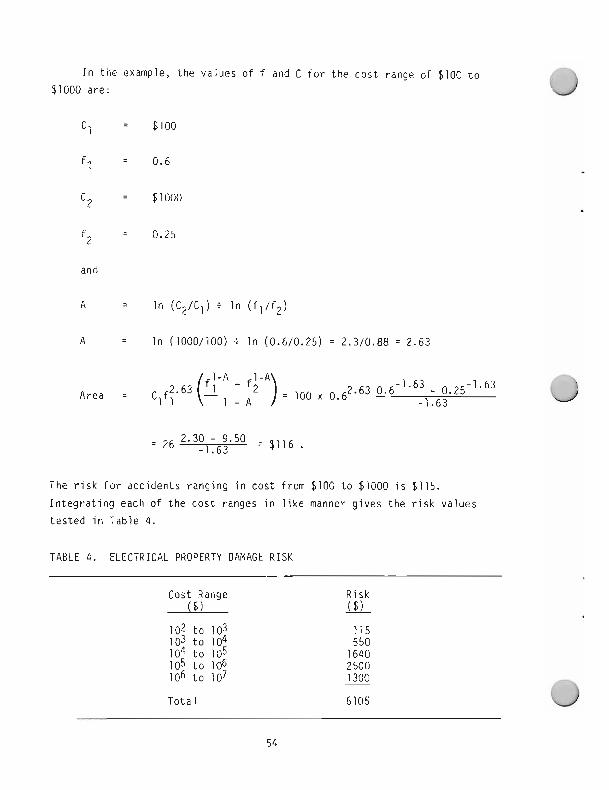
In the example, the values of f and C for the cost range of $100 to $1000 are:

2 = 0.25

and

A = in (C2/C1) t in (fl/f2)

A = In (10001100~ + in (0.610.25) = 2.310.88 = 2.63

f2.63 (f;-A - f;-A) 2.63 0.6- 1.63 - 0.25-1.63 Area = 1 1 1 - A = 100 x 0.6 -1.63

The risk for accidents ranging in cost from 6100 to $1000 is $115. Integrating each of the cost ranges in like manner gives the risk values tested in Table 4.

TABLE 4. ELECTRICAL PROPERTY DAMAGE RISK

Total 6105

The mean o f a c t u a l losses over t h e 5-year p e r i o d i s $66,219 d i v i d e d by

22 o r 63010. The average c o s t of acc idents , from t h e i n t e g r a t i o n which

i nc ludes t h e l a r g e acc iden t which has n o t y e t happened, i s about $6100.

The $6100 i n t e g r a t e d va lue i s t h e b e t t e r es t ima te of t h e mean. The average

number o f acc iden ts i s 22 d i v i d e d by 5 o r 4 .5 lyear . (The f requency i s n o t

a f fec ted by t h e s i z e of t h e acc iden t and can be c a l c u l a t e d d i r e c t l y w i t h o u t

adjustment.)

The i n t e g r a t i o n was te rm ina ted a t $10,000,000 i n Tab le 4. A t t h i s

p o i n t , t h e s lope i s q u i t e s teep and t h e r i s k i n t h e nex t decade would be

Only $100 o r $200. I n a d d i t i o n , t h e d a t a have a l ready been e x t r a p o l a t e d

from $50,000, so t h e u n c e r t a i n t y i s ve ry l a rge .

Judging f rom t h e t a b u l a t e d r i s k va lues f o r each c o s t range, t h e c o s t

range o f maximum r i s k i s $100,000 t o $1,000,000. Th i s i s i n agreement w i t h

t h e conc lus ion t h a t t h e c o s t range of g r e a t e s t r i s k i s where t h e s lope i s

equal t o one, j u s t beyond t h e $100,000 consequence value.

F o r any acc iden t type, i f a s u f f i c i e n t l y l a r g e number o f acc iden ts

have been exper ienced, t h e i n t e g r a t e d mean w i l l be ve ry n e a r l y equal t o t h e

mean c a l c u l a t e d d i r e c t l y f rom exper ience data. For example, a 5-year

average c o s t o f passenger v e h i c l e p r o p e r t y damage f o r one c o n t r a c t o r was

$175. Going through t h i s exe rc i se f o r t h e more than 100 acc iden ts

exper ienced y i e l d e d an i n t e g r a t e d mean o f $174.

I n summary, p l o t t i n g acc iden t d a t a and i n t e g r a t i n g t h e r e s u l t i n g

frequency-consequence curves determine t h e c o s t range of maximum r i s k and

p r o v i d e approximate r i s k values, which a re more accura te t han s imple

p r o j e c t i o n of l a s t y e a r ' s losses. Appendix B p rov ides a d d i t i o n a l d e t a i l

f o r those i n t e r e s t e d i n r i s k p r o j e c t i o n techniques.

6.9 Extreme Value A n a l y s i s

Extreme va lue a n a l y s i s i s d iscussed b r i e f l y i n t h e MORT t e x t , ' ' t h e

A c c i d e n t l i n c i d e n t I n v e s t i g a t i o n ~ a n u a l , " and i n d e t a i l by umbel.' The maximum events taken f rom each o f a l a r g e number of t ime i n t e r v a l s f o rm

a special frequency-severity relationship which is somewhat similar to the

log-normal distribution pattern. The scale on the extreme value graph paper converts this skewed, bell-shaped curve to a straight line on the x-axis.

Also on the x-axis opposite the frequency (cumulative probability) scale is

a scale which converts the frequency to "return periods." This return period is in the same time units as the time intervals from which the maxi-

mum events were taken. The y-axis represents the severity or cost. The average time between events (return period) can be read directly from the

graph paper for maximum events of any given severity or cost. The value lies in the ability to extrapolate or extend the straight line to include

longer time periods, and thus predict the occurrence of very large

accidents.

There are two kinds of extreme value graph paper. On one paper, the

cost scale i s linear; on the other the cost scale is logarithmic. The

reason is that for events resulting from multiple independent causes, the

cost increases linearly with respect to the cumulative probability scale.

For those events resulting from multiple interdependent causes, the cost

increase exponentially or logarithmically. This indicates a possibility of

a common cause, such as some factor in the management system, leading to

the several causes of the large accident.

The extreme value equation is an empirical derivation of the frequency

and severity of maximum events represented on the upper tail of the log- normal curve. The basic difference between extreme value and log-normal

analysis is that all events are used in log-normal analysis, but only the

maximum events are used in extreme value analysis. Extreme value analysis

is generally preferred because: (a) maximum event data are frequently

available when a record of events is incomplete; (b) it is quicker and

easier to use in that less data is involved, and the return period can be

read directly from the graph paper; (c) no judgment is required in plotting

the data, whereas judgment is required in selecting cost intervals in

log-normal analysis.

The log-normal and log-log analyses are required to determine the

relative risk of small versus large accidents and to determine the average

cost of potential accidents.

56

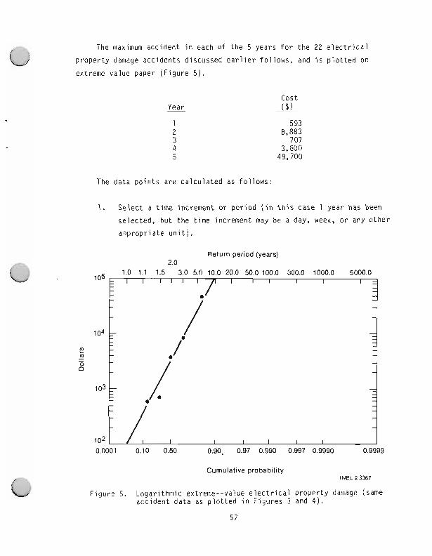
The maximum accident in each of the 5 years for the 22 electrical

property damage accidents discussed earlier follows, and is plotted on

extreme value paper (Figure 5).

Year - cost (4)

The data points are calculated as follows:

1. Select a time increment or period (in this case 1 year has been

selected, but the time increment may be a day, week, or any other

appropriate unit).

Return period (years) 20

Cumulative probability INEL23367

Figure 5. Logarithmic extreme--value electrical property damage (Same accident data as plotted in Figures 3 and 4) .

2. Select the maximum loss event for each time period and rank the

selected events in order of increasing cost.

3. Select a vertical scale which will permit extrapolation to desired consequence levels (generally two to three times the maximum

value).

4. Calculate the cumulative probability by dividing Ni by N + 1.

Note that the five data points (one for each of five years) divide

the cumulative probability scale into N + 1 or six intervals.

The results data are given below:

cost 1BL Ni

(Ni/N + 1) x 100 -

5. Plot the data on both logarithmic and linear extreme value papers and use the paper that gives the best straight-line fit. If a

straight-line relationship does not occur in either case, analyze the data for homogeneity--first by scanning, then by formal

change analysis. 1 1

If the plot approximates a straight line on linear graph paper, the

accidents are likely to be independent and the prevention of extremely

large accidents is well under control. If the plot approximates a straight

line on logarithmic paper, the multiple causes can usually be traced back

to a common source, or one cause influences another. Since a strong systems

control program would eliminate common causes, review of the control or

safety system may be in order. This is especially true if the slope of the logarithmic curve is steep so that the return period for a large accident

is short.

Cor rec t i ons f o r "number of employees" o r company growth shou ld n o t be

made on t h e consequence sca le . It i s n o t reasonab le t o expect t h a t "ha l v -

i n g ' t h e s i z e of an a c t i v i t y would "ha lve" t h e s e v e r i t y of t h e most severe

event . A more reasonab le method f o r making such c o r r e c t i o n s i s t h rough t h e

r e t u r n per iod . That i s t o say, if one has d a t a from an e x i s t i n g u n i t and

adds an i d e n t i c a l u n i t t o t h e system, one would expect t o ha l ve t h e r e t u r n

p e r i o d ( t h e t ime when t h a t consequence event i s expected t o recu r ) . T h i s

i s t h e same as n o r m a l i z i n g t h e raw acc iden t d a t a t o t h e number of employees.

From F i g u r e 5, a r e t u r n p e r i o d o f 10 years i s found f o r a $100,000

acc ident . T h i s i s cons idered t o be good agreement f o r t h e 17-year p e r i o d

us ing a l l 22 acc iden ts on log-normal paper. As d iscussed e a r l i e r , t h e l og -

normal curve e x h i b i t s a dog- leg c h a r a c t e r i s t i c . F i t t i n g a s t r a i g h t l i n e t o

o n l y t h e upper segments w i l l y i e l d a r e t u r n p e r i o d of 10 years.

T h i s i l l u s t r a t e s t h a t t h e upper segment of a dog- leg p r o b a b i l i t y cu rve

p r e d i c t s more a c c u r a t e l y t h e frequency of l a r g e consequence events, and t h a t

I 0 yea rs i s t h e c o r r e c t r e t u r n per iod . However, u n t i l t h e reason f o r t h e

dog- leg i s i d e n t i f i e d , i t shou ld be assumed t h e r e t u r n p e r i o d l i e s i n t h e

range o f 10 t o 17 years . Other examples of extreme va lue p r o j e c t i o n a r e

g i ven i n Appendix 0 .

6.10 F a u l t Tree Ana l ys i s and Other Hazard I d e n t i f i c a t i o n

and Eva lua t i on Techniques

Prepared by P. L. Clemens, Sverdrup Technology Inc. , Arno ld A i r Force

S ta t i on , Tennessee, a l s o a v a i l a b l e from t h e System Safe ty Development Center

i s a Compendium of Hazard I d e n t i f i c a t i o n and Eva lua t i on Techniques f o r

System Safe ty A p p l i c a t i o n . T h i s document p rov ides a b s t r a c t s of 25 d i f f e r e n t

techn iques. Descr ibed a re method, a p p l i c a t i o n , thoroughness, mastery

requ i red , and d i f f i c u l t y o f a p p l i c a t i o n w i t h comments prov ided.

Most of these techn iques a re usefu l i n hazard i d e n t i f i c a t i o n and

systems a n a l y s i s bu t do no t p rov ide a measure o f r i s k . One t h a t does, f a u l t

t r e e ana l ys i s , i d e n t i f i e s one undes i rab le event and t h e c o n t r i b u t i n g

elements ( f a u l t s / c o n d i t i o n s ) t h a t are r e q u i r e d t o p r e c i p i t a t e t h e undes i red

event. These events are arranged in a logic tree and the probability of the top (undesired) event is calculated using network paths through Boclean

Logic gates. A Reliability and Fault Tree Analysis Guide, SSDC-22 is

available. 13

Fault Tree Analysis is time consuming and costly. A major effort is required to prepare and analyze a tree for a single event so that use of

this technique is limited to specific high risk events. A limitation of this technique is that there are inadequate means to assure completeness.

It is impossible to include or arrive at all possible combinations of

events leading to the undesired events (or in other words all possible ways

the undesired event can happen). Of great value is that the sensitivity of

the top event to a particular component failure can be determined and

redundancy or other means taken to make the component failure less

critical. Also, fault tree analysis greatly increases the understanding of a system and how the various components interact, especially during failure.

7. CONSEQUENCE ANALYSIS

The identification of accident consequences and quantification of the

associated risk serves two purposes. The identification permits control measures to be designed and applied. The risk quantification helps deter-

mine whether the risk is serious enough to warrant control measures. (The

risk reduction should be balanced against the costs of additional control

measures.) In the accident cost analysis, there are two dimensions that

must be considered:

1. Types of consequences (property, environment, and human)

2. Indirect costs (lost time, administrative, legal, and replacement

of services or products).

Both dimensions must be considered if the risk assessment is to be

complete and various types of consequences are to be treated equally on a

systematic basis.

The simplest way to treat the various types of consequences is to sim-

ply assign units to each of the identified consequences. Monetary units

(dollars) have the distinct advantage of permitting a direct comparison of

the dollar cost of risk reduction against the expected loss. These are

terms a program manager can easily understand. A disadvantage is there may be a negative reaction when placing a dollar value on human life or

environmental values.

It may be argued that assigning a cost for a fatality is not placing a

value on life but is placing a standard value to help allocate safety

resources efficiently so that loss of life may be minimized. Nevertheless,

there will still be those who object. If dollar values are used, they

should be stated in the risk document in such a way that the risk values can

be easily revised based on different dollar values for intangible effects.

Merely assigning arbitrary units to intangible effects results in risk

values expressed in arbitrary units which are useful only for comparing one

type of risk to another. The arbitrary units may be summed and then con- verted to dollars, but this is a thinly disguised method of assigning dollar

values.

Another method of dealing with the problem is to classify consequences

by ranges of severity such as A, B, or C events; with A being the worst accident to occur and C the least severe. The following values have been proposed: 5

1. Loss of Life

A event--30 fatalities

B event--5 to 29 fatalities

C event--1 to 4 fatalities

2. Environmental Pollution

A event--10 million tons oil spilled

B event--100,000 to 10 million tons oil spilled C event--1,000 to 100,000 tons oil spilled

3. Property Loss

A event--2 billion dollars

B event--20 million to 2 billion dollars C event--200 thousand to 20 million dollars.

By equating A, 8, and C events, equivalent dollar values can be obtained for oil spills and fatalities (human life). In doing so, an inconsistency will be obvious. The dollar value per life is $67 million

for B events and $200 thousand to $4 million for C events.

To avoid assigning dollars to each of these three types of losses, it

has been suggestedi4 risks be presented in all three dimensions (human,

environment, and property) all the way to the decisionmakers.

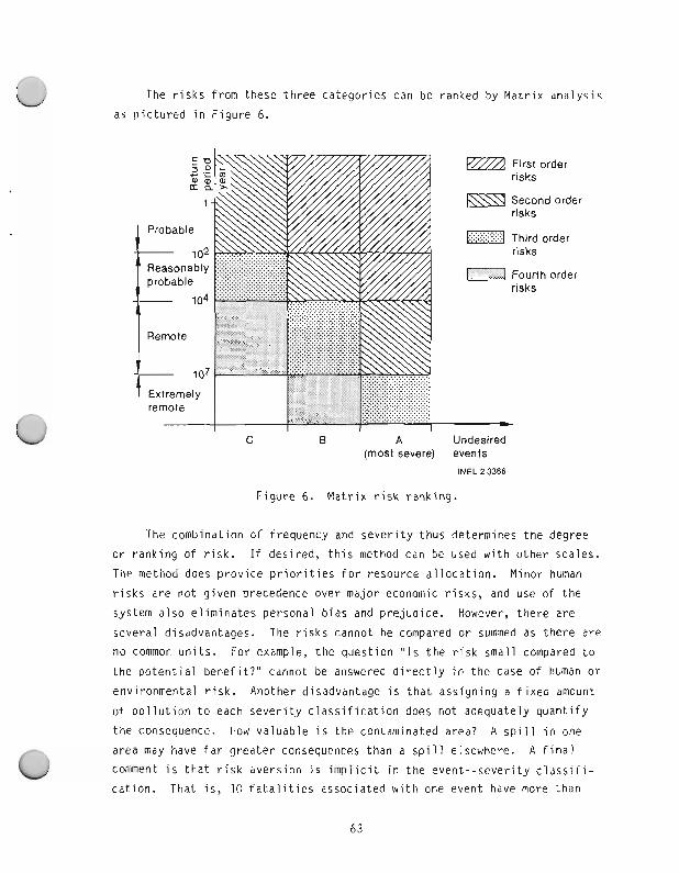
The r i s k s f rom these t h r e e ca tego r i es can be ranked by M a t r i x a n a l y s i s

as p i c t u r e d i n F i g u r e 6.

First order risks

Second order risks

r"l Fourth order rlsks

C A Undesired (most severe) events

INEL23366

F i g u r e 6. M a t r i x r i s k rank ing.

The combinat ion of f requency and s e v e r i t y t hus determines t h e degree

o r r a n k i n g o f r i s k . I f des i red, t h i s method can be used w i t h o t h e r sca les .

The method does p r o v i d e p r i o r i t i e s f o r resource a l l o c a t i o n . Minor human

r i s k s a re n o t g i ven precedence over major economic r i s k s , and use o f t h e

system a l s o e l i m i n a t e s persona l b i a s and p re jud i ce . However, t h e r e a re

seve ra l d isadvantages. The r i s k s cannot be compared o r summed as t h e r e a r e

no common u n i t s . For example, t h e ques t i on " I s t h e r i s k smal l compared t o

t h e p o t e n t i a l b e n e f i t ? " cannot be answered d i r e c t l y i n t h e case of human o r

env i ronmenta l r i s k . Another disadvantage i s t h a t ass ign ing a f i x e d amount

of p o l l u t i o n t o each s e v e r i t y c l a s s i f i c a t i o n does n o t adequately q u a n t i f y

t h e consequence. How va luab le i s t h e contaminated area? A s p i l l i n one

area may have f a r g r e a t e r consequences than a s p i l l elsewhere. A f i n a l

comment i s t h a t r i s k ave rs ion i s i m p l i c i t i n t h e e v e n t - - s e v e r i t y c l a s s i f i -

ca t i on . That i s , 10 f a t a l i t i e s assoc ia ted w i t h one event have more than

10 times the consequence of one fatality; thus, relatively more should be done to protect groups than individuals. From the individual's viewpoint,

it may make no difference whether others are killed with him; and thus, the

risk should be linear. From an organizational viewpoint, risk aversion

should be based on its impact on the organization. While many questions

have been raised, no answers are provided in this document. These questions

should be addressed in the formulation of a risk management program when establishing goals and acceptable levels of risk. It may be that flexibil- ity is desired in that dollar values for environmental effects or human

life are acceptable in some situations, but not others. Consideration of

risk aversion and/or discounting future loss/benefits to present values may

be desirable at times. In any event, the consequence and associated unit

of risk should be explicitly stated in a risk assessment document.

7.1 Direct and Indirect Accident Costs

Direct and indirect costs should be assessed in light of the conse-

quences discussed above. For a specific hazard, the various possible

consequences and their costs could be evaluated on an individual basis.

Costs for cropland destroyed could be based on the annual value of the

crops or the market price of the land. Pollution could be measured by

economic losses due to sickness or illness, plus a factor for human misery

associated with illness.

Much time can be saved if only direct costs are considered and a

multiplying factor is used for the indirect costs. This has an averaging

effect which is not detrimental because while indirect costs may vary

greatly, the probable value is, by definition, equal to the average

indirect cost.

There is no logical basis for separating accident consequences into

"direct" and "indirect" costs. However, a number of s t ~ d i e s l ~ " ~ ' ~ ~ have

been made to determine the "direct/indirectU or the "visible/hiddenU acci-

dent cost ratio. Usually, the purpose is to determine the total to accident

cost. For this same reason, we have labeled accident consequences which

are normally reported as "direct" costs, although this is strictly a

Convent ion used t o a r r i v e a t t h e t o t a l r i s k w i t h o u t reco rd ing a l l of t h e

consequences f o r eve ry acc ident . (A more accu ra te d e s c r i p t i o n o f d i r e c t /

i n d i r e c t cos t s might be " repo r ted " and "no t repo r ted . " ) Each company

shou ld determine t h e i r own d i r e c t and i n d i r e c t c o s t r a t i o , s i nce bo th

d e f i n i t i o n s and a c t u a l r a t i o s w i l l vary.

Acc ident losses no rma l l y r e p o r t e d are :

1. The amount of f i r s t aid, medica l t rea tment , workdays l o s t , and

f a t a l i t y cases

2. The number of and d o l l a r damage amount f o r v e h i c l e acc idents ,

p r o p e r t y damage, and f i r e s .

The balance of t h i s chap te r d iscusses methods f o r de te rm in ing t h e

d i r e c t and i n d i r e c t acc iden t cos t s s t a r t i n g f rom those losses no rma l l y

repor ted. The a c t u a l data, c a l c u l a t i o n s , and r e s u l t s of a DOE c o n t r a c t o r

exper ience are presented f o r i l l u s t r a t i v e purposes. The cos t o f each t y p e

of l o s s and t h e number of acc iden ts w i l l va ry w i t h i n d i v i d u a l o r g a n i z a t i o n s

and w i t h i n f l a t i o n . (Each o r g a n i z a t i o n shou ld eva lua te t h e i r own c o s t s and

numbers of acc idents . ) A summary of these d a t a i s g i ven i n Tab le 5. As

can be seen, t h e d i r e c t c o s t i s ob ta ined by m u l t i p l y i n g t h e average c o s t by

t h e number o f acc idents . The va lues i n Table 5 a re n o t t h e same as would

be ob ta ined f rom adding t h e cos ts of a l l acc iden ts because: ( a ) t h e r e a re

no " repo r ted " c o s t va lues f o r i n j u r i e s and f a t a l i t i e s , ( b ) f r a c t i o n a l num-

be r of cases, such as 0.06 f a t a l i t i e s , a re es t ima ted (none had occur red) ,

and ( c ) t h e average c o s t of p r o p e r t y l o s s was es t ima ted f rom log-normal

a n a l y s i s of each t ype o f p r o p e r t y l o s s acc ident , as exp la ined e a r l i e r i n

t h i s chapter .

The i n d i r e c t c o s t m u l t i p l e i s t h e sum o f t h e d i r e c t c o s t and t h e

i n d i r e c t c o s t d i v i d e d by t h e d i r e c t cos t . M u l t i p l y i n g t h e average d i r e c t

c o s t pe r acc iden t by t h i s m u l t i p l i e r g i v e s t h e t o t a l c o s t p e r acc ident , o r

(as i n t h e t a b l e ) m u l t i p l y i n g t h e d i r e c t annual c o s t of a c l a s s o f acc iden ts

g i ves t h e t o t a l annual c o s t of t h a t c l a s s of acc idents . These m u l t i p l i e r s should no t change w i t h i n f l a t i o n and may be used i n l i e u of making i n d i r e c t

TABLE 5. DIRECT AND INDIRECT ACCIDENT COSTS

Acc ident Category

I n j u r y

F i r s t - a i d , o n - s i t e med ica l O f f - s i t e medica l Workdays l o s t F a t a l i t y

T o t a l i n j u r y m m Prope r t y

I n - p l a n t 61000 I n - p l a n t $1000 V e h i c l e F i r e

T o t a l p r o p e r t y

T o t a l of i n j u r y and p r o p e r t y

Average D i r e c t Cost /Acc ident

( 9 )

a. T h e o r e t i c a l va lue on l y ; no death recorded.

D i r e c t Annual

Number o f "liar Cos: I n d i r e c t Cost T o t a l Cost x 10 3

Cases/Year ( r i s k x 10 ) M u l t i p l i e r ( $ )

c o s t s t u d i e s f o r t h e acc ident c lasses cons idered i n Table 5 f o r you r own

o r g a n i z a t i o n . They a re b e l i e v e d t o be conse rva t i ve i n t h a t o n l y those

i n d i r e c t f a c t o r s which were i d e n t i f i e d and eva luated are i nc luded i n

Tab le 5.

7.2 D i r e c t Acc ident Costs

7.2.1 F i r s t Aid, On-Si te Medica l

The c o s t f o r f i r s t a i d and o n - s i t e medica l t r ea tmen t was es t imated by

t h e medica l d i r e c t o r t o be $lO/case. (On-Site medica l t r ea tmen t c o s t s a re

c l o s e r t o f i r s t a i d cos t s p r i m a r i l y because of t r a v e l t ime. I n a d d i t i o n ,

o f f - s i t e cases a re p a i d f o r t h rough workmen's compensation as t h e y a re

t r e a t e d by a 'noncompany" doctor . )

7.2.2 O f f - S i t e Medica l

For t h e DOE c o n t r a c t o r , o f f - s i t e medica l t r ea tmen t p a i d t h rough work-

men's compensation c o s t s $60/case, averaged over a severa l yea r per iod .

7.2.3 Workdays L o s t

Costs which appear i n t h e company's f i n a n c i a l records a re t h e medica l

cos t s and t h e i n j u r e d employee's wages p a i d t h rough workmen's compensation.

I t i s noted t h a t t h e p a r t of t h e employee's wages p a i d t h rough s i c k leave

b e n e f i t s w i l l va ry w i d e l y from one s t a t e t o t h e next. If s i c k leave bene-

f i t s become exhausted, p a r t of t h e l o s s may be borne by t h e i n j u r e d

employee. For t h i s r e p o r t , d i r e c t cos t s f o r l o s t t i m e i n j u r i e s a re def ined

as medica l c o s t s p l u s wages p a i d t o t h e employee from b o t h s i c k leave and

workmen's compensation. Th i s was assumed t o average $1200 f o r medica l

Costs and $2300 f o r wages, o r a t o t a l d i r e c t c o s t of $3500/accident. (Th i s

assumption i s based on t h e c o n t r a c t o r ' s exper ience. Since t h i s c o n t r a c t o r

has a s e v e r i t y r a t e much lower t han t h e average DOE c o n t r a c t o r , each

Con t rac to r shou ld determine t h e i r cost . )

7.2.4 Fatality Costs

The dollar value for a fatality is very subjective. A number of papers have been written on this subject. 15'16'18 Estimates have been based on:

1. Future earnings

2. Propensity or willingness to accept risk in return for some

benefit

3. Wage differential for highllow risk operations

4. Direct company costs, such as death benefits (insurance and

replacement expenses).

All such analyses contain serious deficiencies. There is no consensus

on whether the losses should be determined from a society, company, or

individual viewpoint. In addition, it is the company which accepts the

residual risk, but the majority of the losses are suffered by the injured

employee and his dependents. The loss to society is usually considered

fairly insignificant for a single individual, since the average person

consumes much of what he produces. However, the economic cost to society

resulting from the death of an employee with many dependents may be very large. Attempting to determine the dollar value of a human life from voluntary risk acceptance patterns is not practical, because individual

Perceptions of risk acceptability are extremely variable and it is difficult

to determine whether the occupational risks are really understood by the

worker (and, consequently, whether they are voluntary or involuntary).

Within a company, the costs for the loss of an employee also vary

greatly. It would undoubtedly have a much greater effect on any company to

lose a key scientist or executive than an average employee. For specific

risk analysis where only management personnel are at risk, such as corpo-

rate aircraft travel hazards, a million dollars per life may not be too

high. Yet, $100,000 for the average employee is believed to be higher than the actual dollar costs to a contractor. Most of the studies referenced

previously arrive at a dollar value for human life in the range of $100,000

to $500,000. While it is evident that values in this range cannot be jus- tified for the average employee solely on a company economic basis, most of

those who have considered the problem believe that economics should not be

the sole basis. Currently, there are large differences in explicit or

implicit values applied by different regulatory agencies and individual

analysts. The most valid basis appears to be a consensus of informed

employers and workers who must bear the risk and pay for risk control.

Unfortunately, such a consensus is not available. Nevertheless, if a consistent value is used by all DOE contractors, risk studies could be

compared on a consistent, relative basis.

A fatality cost of $200,000 was arbitrarily selected for use in this guide. (For directfindirect cost analysis, $100,000 is assigned to direct

costs and $100,000 to indirect costs.) Lifetime earnings could be used,

which would result in, perhaps, $500,000 for computational purposes.

While it may seem distasteful to place a dollar value on a human life,

no other scale appears adequate to provide a direct comparison of the risks

and the resources allocated to risk reduction. In addition, the use of

almost any yardstick (even placing a dollar value on human life) seems pre-

ferable to the usual practice of allocating finite resources to lifesaving

measures on a completely arbitrary and subjective basis.

The contractor being used as an example had never experienced an occu-

pational fatality. The fractional number of fatal cases per year was

derived as follows. The National Safety Council and company safety records

give the following national and company vehicle accident data:

e Company vehicle mileage = 1.7 n lo6 mileslyear

6 a Company accident rate = 6.4/10 motor vehicle miles

6 e National accident rate = 19/10 motor vehicle miles

8 e National death rate = 1.3/10 passenger miles

r Assumed number of passengers per vehicle = 2

r National rate of injuries per fatality = 37

-8 deaths 10-6 miles r P = 1.3 x 10 - mile year

X 6.4 x company accident rate

19 10-6 national accident rate x 2-

x 1/2 seat belt factor = 0.008 fatalitieslyear. a

The probability of a lost time injury from a vehicle accident is:

P = 37 injurieslfatality x 0.008 fatalitieslyear = 0.3 injurieslyear.

These theoretical probabilities should be added to the other

theoretical probabilities, and the actual number of fatalities or lost time

injuries should be related to other accidents to obtain the expected or

average number per year for all company accident types.

7.2.5 Property Damage

Direct costs of property damage accidents are defined by DOE to

include labor and material for replacement and cleanup costs. Depreciation

adjustments are not made. Average direct costs can be derived by

separating property damage and vehicle cases into proper categories, and by

dividing the total cost in each category by the number of cases in that

category. This gives a measurement only of accident costs experienced to

date. It does not provide a risk measurement of the large accident which

has not yet happened. Adjustments to include the large consequence

potential should be made as discussed in detail in Section 6.

a. The 1/2 factor is for greater use of seat belts by company employees.

7.3 Indirect Costs

For each of the categories discussed under Direct Costs and in

Table 5, indirect costs were evaluated. These values were used to derive

the indirect cost multipliers as explained, which were evaluated separately

for each category and also at different severity levels, because indirect

cost factors are not a linear function of severity.

Indirect cost items have been identified. These are believed to

include nearly all of the hidden costs for each of the accident categories listed in Table 5. However, not all of the items are applicable to all

categories; for example, there are no new employee training costs for first

aid cases. The items are discussed on the following pages.

7.3.1 Injured Worker Time

Productive time is lost by injured employee and is not reimbursed by

workmen's compensation.

7.3.2 Co-Worker Time

1. Time is lost by co-workers at the scene, as well as when assisting

the injured to dispensary or ambulance.

2. Time is lost through sympathy or curiosity, and work interruption

at the time of injury and later from discussing the case, telling

similar stories, swapping opinion of cause, grumbling, etc.

3. Incidental lost time results from cleanup, collecting donations

to aid the employee and his family, review hearings, etc. The

cost of other employee overtime required to accomplish the

injured employee's work and the time spent by safety organization

personnel on the accident should be included.

Superv i so r t ime charged t o t h e acc iden t shou ld i nc lude :

1. A s s i s t i n g i n j u r e d employee

2. I n v e s t i g a t i n g acc iden t cause, i.e., i n i t i a l i n v e s t i g a t i o n ,

fo l lowup, research on prevent ion , etC.

3. Ar rang ing f o r work cont inuance, g e t t i n g new m a t e r i a l , r eschedu l i ng

4. S e l e c t i n g and t r a i n i n g new employee; i n c l u d i n g o b t a i n i n g

app l i can ts , e v a l u a t i n g candidates, and t r a i n i n g new employee o r

t r a n s f e r r e d employee

5. P repa r i ng acc iden t r e p o r t s

6. P a r t i c i p a t i n g i n hear ings o r c o u r t proceedings.

7.3.4 General Losses

1. P roduc t i on t i m e i s l o s t due t o upset, shock, o r d i v e r t e d i n t e r e s t

of workers, slowdown of o thers , d i scuss ion by o the rs - - "d id you

hea r . . . " - - (app l i es t o employees o f o t h e r u n i t s n o t i nc luded i n

I t em 3, on t h e p rev ious page)

2. Losses r e s u l t from work stoppage o f machines, veh i c l es , p l a n t s ,

f a c i l i t i e s , etc., and can be e i t h e r temporary o r l ong te rm and

e f f e c t r e l a t e d equipment and schedules

3. The i n j u r e d employee's e f fec t iveness i s o f t e n reduced a f t e r h i s

r e t u r n t o work, f r om work r e s t r i c t i o n s , reduced e f f i c i ency ,

p h y s i c a l handicaps, c ru tches, s p l i n t s , e t c .

4. Loss of business and goodw i l l , adverse p u b l i c i t y , problems i n

o b t a i n i n g new h i r e s , etc., a re common genera l lOSSeS

5. Legal expenses arise from compensation hearings, liability claims handling, etc., that involve contractor legal services, rather

than the insurance carrier legal expense that appears in direct

costs

6. Costs can increase for insurance reserves and tax multipliers

which are, respectively, small annual percentages of the gross

incurred losses, and taxes based upon the dollar value of losses,

that are tied up in reserves

7. Replacement of services or products loss during downtime and/or

penalties administered under penalty contract clauses for DOE

contractors

8. Miscellaneous additional items should be included which may be unique to particular operations and are appropriate to specific

accident cases.

An average value for each of the above items can be estimated for each

of the categories in Table 5. The sum of these values for each category is

the total indirect cost. The sum of the indirect and direct cost, divided

by the direct cost gives the indirect cost multipliers listed in Table 5.

This indirect cost multiplier, as used in Table 5, gives the total annual cost of accidents when multiplied by the annual direct cost of accidents.

(The multiplier could first be applied to the direct cost of each accident,

and then the total cost of each accident multiplied by the annual number of

accidents.)

Evaluating the indiviaual items for each category is not simple. The

results in Table 5 are our best estimates based on the results of:

1. An opinion survey of 35 supervisors

2. Field evaluations of accidents as they occur

0 3. Legal and financial records.

The opinion survey gave inflated results. For example, in 1976, 35 supervisors, when given the items and a description of a first aid case

i- L

to evaluate, estimated losses ranging from $75 to $1490. On the other hand, costs for 1 1 first aid cases were evaluated jointly by safety

engineers and supervisors as they occurred. Their estimates ranged from $5 to $80 with an average of $30 per case. In general, the indirect costs do not appear to escalate linearly with severity. This confirms the need

for evaluating indirect costs separately for different severity levels.

Items which are determined directly, such as legal expense or insurance Costs, should not be included in an opinion survey, but should be taken

directly from appropriate records. In addition, personnel making the

evaluation should make estimates in hours for lost time accompanied by

descriptive information, such as "reactor shutdown for 2 hours."

Conversion to dollar values should then be made by one person with adeauate

cost and salary information. Estimates of general losses should be

submitted directly in dollar values.

Once the evaluation has been made, the indirect cost multiplier can be

used for several years, although periodic ref inement is recommended. It is C

emphasized that the indirect multipliers in Table 5 need further field

evaluation and should not be accepted as more than gross approximations.

However, Table 5 does provide one way to compile total accident costs for

any company.

8. RISK ASSESSMENT OF EXISTING SYSTEMS

A risk assessment of the total operations for an existing company

serves several purposes.

1. Oversights are identified. In one case, a risk assessment

resulted in adding a needed electrical engineer to the safety

staff.

2. Assurance is provided that adequate safety control is being

maintained.

3. The various risks are placed in perspective for management.

Resources can be adjusted for cost effectiveness.

4. Areas where regulations are either less than or more than adequate

can be identified. The single minded application of regulations

frequently result in the wasting of resources where little real

risk exists. Waivers, exemptions, or changes in the regulations should be granted wherever it is clear that little benefit is

derived. Risk assessment provides continual feedback to adminis-

trators to make regulations more effective and cost efficient.

8.2 Risk Identification and Rankinq

A systematic search for all risks greatly reduces the number of hazards

which will be neglected because of management oversight. Based on the

premise that all accidents result from an unplanned and unwanted transfer

of energy, the Risk Identification Tree was developed by Dr. R. J. Nertney of the EG&G Idaho System Safety Development Center and is presented in

Appendix A.

Another method for identifying hazards is to use a process called a

Reported Significant Observation (RSO) study. An RSO study is an

in fo r rnat ion-gather ing method which use employee-par t ic ipants t o d e s c r i b e

s i t u a t i o n s t h e y have p e r s o n a l l y wi tnessed, i n v o l v i n g good and bad p r a c t i c e s

and safe and unsafe cond i t i ons . T h i s i n fo rma t i on i s u t i l i z e d i n t h e r i s k

assessment process t o h e l p m o n i t o r t h e presence of hazards, and the reby

he lp e l i m i n a t e them and p reven t t h e i r ex i s tence i n f u t u r e ope ra t i ons and

designs. One such RSO s tudy i d e n t i f y i n g h i g h r i s k energy types was com-

pared t o a c t u a l AEC f a t a l i t i e s by energy type. The e x c e l l e n t agreement

demonstrates t h a t RSO s t u d i e s can be h i g h l y accura te i n p r e d i c t i n g areas

o f h i ghe r t han average r i s k .

T h i s c o n s t i t u t e s a rud imentary i d e n t i f i c a t i o n and rank ing o f r i s k s .

The r i s k s can be f u r t h e r q u a n t i f i e d from a c t u a r i a l d a t a and t h e o r e t i c a l

es t imates . The genera l method i n p r i n c i p l e i s q u i t e s imple: determine t h e

average annual c o s t of acc idents , as i n t h e p rev ious sec t i on , and add t o

these c o s t s t h e t h e o r e t i c a l r i s k s no t represented i n t h e a c t u a l l o s s data .

S p e c i f i c s teps which w i l l accompl ish t h i s a re :

1. Choose an acc iden t c l a s s i f i c a t i o n . A l though o t h e r c l a s s i f i c a t i o n s

m igh t be used, we suggest c l a s s i f y i n g by t y p e of energy as g i v e n

i n Table 6. The reasons f o r choosing energy are :

a. Each t y p e of energy c r e a t e s a homogeneous c l a s s of acc iden ts

which increase t h e accuracy o f t h e f r equency -seve r i t y

ana l ys i s . A heterogeneous group o f acc iden ts may comp le te l y

mask t h e p o t e n t i a l f o r a l a r g e acc iden t i n one energy group

if t h e energy group has few acc idents .

b. Energy sources are e a s i l y i d e n t i f i e d so t h a t o v e r s i g h t s a r e

minimized. A thorough hazards i d e n t i f i c a t i o n may i n c l u d e a

search of energy sources w i t h i n each f a c i l i t y o r department.

C. The energy types can be grouped by s a f e t y d i s c i p l i n e ( i ndus -

t r i a l , nuc lear , t r a f f i c , f i r e , i n d u s t r i a l hygiene, e t c . ) so

t h a t sa fe t y resource a l l o c a t i o n can be compared t o and

balanced w i t h r i s k s f o r a more c o s t e f f e c t i v e sa fe t y Program.

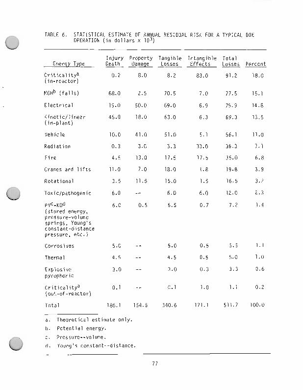
TABLE 6. STATISTICAL ESTIMATE OF ANNUAL RESIDUAL RISK FOR A TYPICAL DOE OPERATION (in dollars x lo3)

Energy Type Injury Property Tangible Intangible Total Death Damage Losses Effects Losses Percent

Criticalitya (in-reactor)

M G H ~ (falls)

Electrical

Kinetic/linear (in-plant)

Vehicle

Radiation

Fire

Cranes and lifts

Rotational

PV C - K D ~ (stored energy, pressure-volume springs, Young's constant-distance pressure, etc.)

Corrosives

Thermal

Explosive pyrophoric

Criticalitya (out-of -reactor)

Total

a. Theoretical estimate only. b. Potential energy.

c. Pressure--volume. d. Young's constant--distance.

2. Ass ign each acc iden t which occur red d u r i n g t h e p a s t severa l y e a r s

t o one of t h e c l a s s i f i c a t i o n s . I n j u r y , p r o p e r t y damage, and

v e h i c l e acc iden ts should be c l a s s i f i e d sepa ra te l y (no te t h a t a l l

v e h i c l e acc iden ts can be cons idered a s p e c i a l case o f l i n e a r -

k i n e t i c energy) . If i n j u r y logs c o n t a i n i n s u f f i c i e n t i n fo rma t i on ,

t h e energy c l a s s i f i c a t i o n may be q u i t e s u b j e c t i v e .

3. Review separa te ly , t h e i n j u r y , veh i c l e , and p r o p e r t y damage

acc iden ts i n each energy c l a s s i f i c a t i o n .

a. If t h e r e a re s u f f i c i e n t data, do a f r equency -seve r i t y ana l y -

s i s , and use t h e i n t e g r a t e d va lue as t h e average c o s t o f an

acc ident . M u l t i p l y t h i s average c o s t of an acc iden t by t h e

average number of acc idents p e r yea r t o o b t a i n t h e average

o r probab le l o s s pe r year . Th i s expected l o s s i s t h e most

l i k e l y c o s t f o r any g i v e n y e a r and i s t h e r i s k f o r t h i s

ca tego ry o f acc idents .

If i t i s assumed t h a t t h e s e v e r i t y d i s t r i b u t i o n of i n j u r i e s

i s t h e same f o r each energy source, t h e c o s t es t ima tes f o r

i n j u r i e s can be made on t h e b a s i s o f t h e number of i n j u r i e s

i n each energy category.

b. I f t h e r e have been few o r no acc iden ts i n a g i v e n category ,

make a t h e o r e t i c a l r i s k es t imate . M u l t i p l y t h i s p r o b a b i l i t y

b y t h e es t imated c o s t t o o b t a i n t h e r i s k f o r t h i s category.

Examples a re g i ven f o l l o w i n g I tem 5 below.

4. En te r t h e " c o s t ' o r r i s k f o r each energy ca tego ry by i n j u r y and

p r o p e r t y damage as i n Table 6. Sum t h e va lue t o o b t a i n t h e t o t a l

t a n g i b l e annual r i s k f o r t h e e x i s t i n g company o r system.

5. Add i n t a n g i b l e acc iden t cos ts . Value f a c t o r s shou ld be added t o

va r i ous energy r i s k ca tego r i es . These a r e based on s u b j e c t i v e

judgment o f t h e a c c e p t a b i l i t y o f d i f f e r e n t k i nds of r i s k . AS

such, adding va lue f a c t o r s shou ld be cons idered a form of r i s k

evaluation rather than risk analysis or quantification. These intangible costs should not include any consequences included in

direct or indirect costs. Intangible costs are primarily nonphysical in nature.

For the study in Table 6, an intangible value factor of 10 for radia- tion categories was selected because of the extreme public reaction (and

the resulting reflection on the nuclear industry) which usually results from an accident involving radiation. Since a fire may or may not involve

radioactive materials, the intangible loss from fires was assumed to be

equal to the tangible loss (a value factor of 1).

A value factor of 1 was also assumed for the toxic/pathogenic cate-

gory. This is both prudent and reasonable, since latent i l l effects of

toxic exposure are not likely to be immediately detected. Intangible costs for all other energy categories were assumed to be 1/10 of tangible costs.

These value factors are arbitrary but were selected only after discussion with DOE and contractor safety personnel. The intangible costs derived

from these factors are given in Table 6.

It is recognized that all intangible risk factors have not been

included. One notable example is that a single, large consequence event is

usually more undesirable than many small consequence events. Witness the

general public acceptance of 50,000 annual vehicle deaths compared to the concern for a maximum potential nuclear reactor accident. In addition, no

attempt has been made to place dollar values on peace of mind, employee

morale, human suffering, etc. All factors included in an assessment should

be explicitly stated. Presentation of risk information should be in a form

which permits ready identification and selection of appropriate factors for

inclusion in the final risk values. However, the limited development of

intangible value factors is considered acceptable for the purposes of this

report. The total losses given in Table 6 are not a dollar value of all

losses, nor indeed can a dollar value be truly placed on esthetic, moral,

or life values. As such, it is emphasized that these risk values are not

absolute or complete risk values. They do place various kinds of risks in

perspective to assure that all risks are managed and accepted in a rational,

systematic manner. In addition, the risk values enable management to com-

pare resources allocated to various risks in a scientific manner.

8.3 Theoretical Risk

TO complete the risk picture so that comparisons in Table 6 are valid theoretical derivation of risk is needed where actuarial data (experience)

is lacking. A reasonable approximation of risk is better than no informa- tion. Examples of theoretical derivations and discussions of some of the

energy categories in Table 6 are given below.

1. Radiation Risk--The radiation risk was subdivided into ''critica-

lity (in-reactor)," "criticality (out-of-reactor)," and "radia-

tion" to correspond with the reactor safety, criticality safety,

and health physics disciplines. Fatality and injury costs from

accidental exposure are assessed in the same way as injury from

other types of energy. (The number of injuries or fatalities is

multiplied by the same average cost of injuries or fatalities as

given for other conventional forms of risk.) These are $100,000

for a fatality and $3500 for the average workday lost injury.

These values are multiplied by the indirect factor of 2 to obtain the total tangible radiation accident costs. To account for the

intangible factors these values are multiplied by 10 to obtain

the total expected loss.

The annual probability of a radiation fatality or injury for a

typical contractor was calculated from the accident data 17

given in Table 7.

These 41 accidental exposures occurred over a 32-year period.

The annual probability for a typical contractor with 2.5% of the

work force would be these values divided by 32 and multiplied by

0.025. Credit should also be taken for improved safety perform-

ance. Of the 41 exposures, 34 occurred during the first 15 years and only 7 during the last 15 years. Using a conservative factor

of 2 for time improvement and the consequence values of $200,000

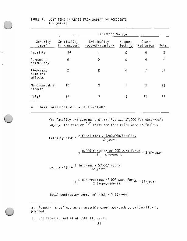
TABLE 7. LOST TIME INJURIES FROM RADIATION ACCIDENTS (31 years)

Severity Level

Fatality

Permanent disability

Temporary clinical effects

No observable effects

Total

Radiation Source

Criticality Criticality Weapons Other (in-reactor) (out-of-reactor) Testing Radiation Total

2a 1 0 0 3

a. Three fatalities at SL-1 are excluded.

for fatality and permanent disability and $7,000 for observable

injury, the reactor a'b risks are then calculated as follows:

Fatality risk = 2 fatalities x $200,00O/fatality

32 years

0.025 fraction of DOE work force = 0,60/year X 2 (improvement)

Injury risk = 2 injuries x $7000/injury

32 years

X 0.025 fraction of DOE work force =

2 (improvement) @/year

Total contractor personnel risk = $166/year.

a. Reactor is defined as an assembly where approach to criticality is planned.

b. See Pages 43 and 44 of SSDC 11, 1977.

81

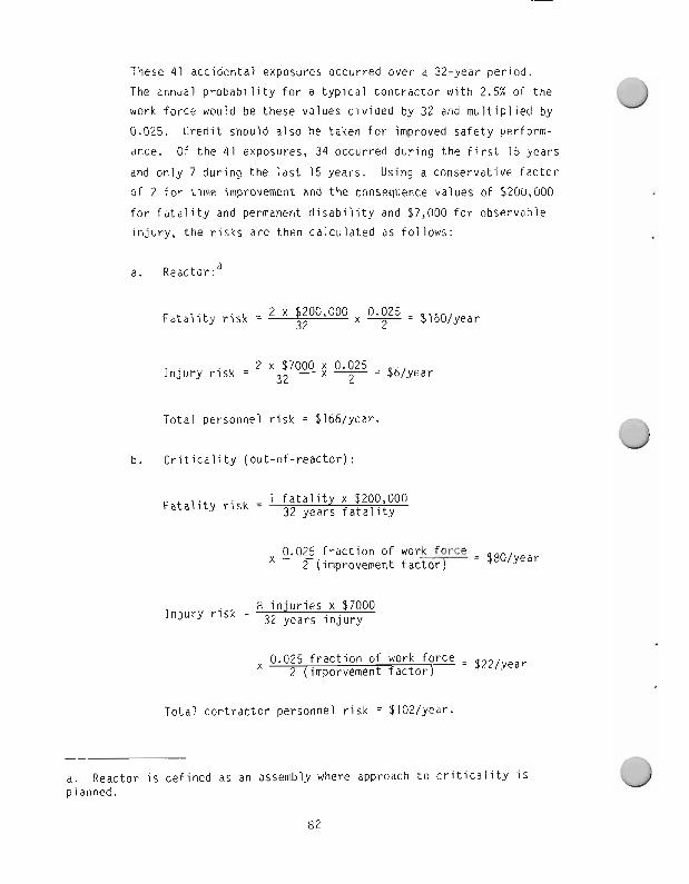
These 41 accidental exposures occurred over a 32-year period.

The annual probability for a typical contractor with 2.5% of the

work force would be these values divided by 32 and multiplied by

0.025. Credit should also be taken for improved safety perform-

ance. Of the 41 exposures, 34 occurred during the first 15 years

and only 7 during the last 15 years. Using a conservative factor

of 2 for time improvement and the consequence values of $200,000

for fatality and permanent disability and $7,000 for observable

injury, the risks are then calculated as follows:

Fatality risk = !;OO'OOO x 9 = $160/year

Total personnel risk = $166lyear.

b. Criticality (out-of-reactor):

X 0.025 fraction of work force _

2 (improvement factor) - $80/year

8 in'uries x $7000 Injury risk = 32 Jyears injury

0.025 fraction of work force = 9221year 2 (imporvement factor)

Total contractor personnel risk = JlOZlyear.

a. Reactor is defined as an assembly where approach to criticality is planned.

82

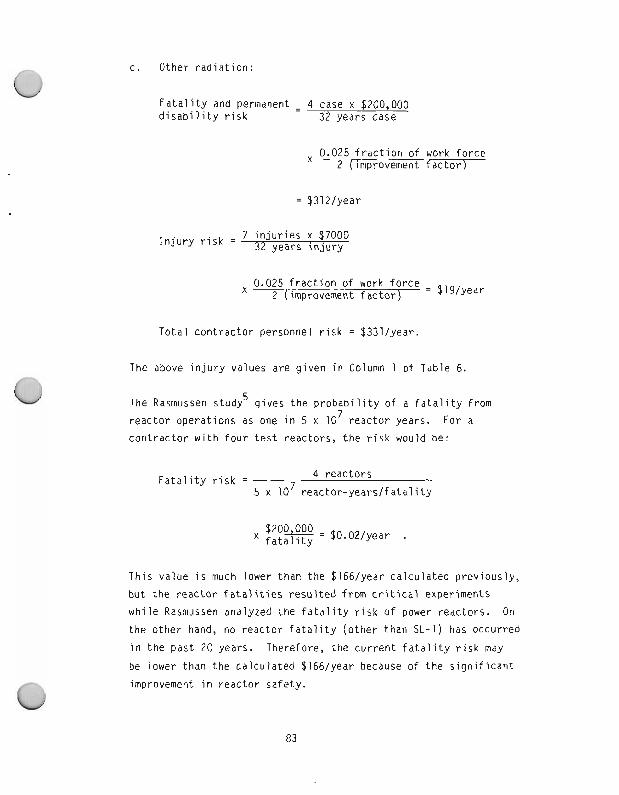
c. Other radiation:

Fatality and permanent = disability risk

4 case x $200,000 32 years case

0.025 fraction of work force 2 (improvement factor)

Injury risk = 7 injuries x $7000

32 years injury

0.025 fraction of work force = $191year 2 (improvement factor)

Total contractor personnel risk = 9331lyear.

The above injury values are given in Column 1 of Table 6.

5 . The Rasmussen study glves the probability of a fatality from 7 reactor operations as one in 5 x 10 reactor years. For a

contractor with four test reactors, the risk would be:

4 reactors Fatality risk = 7 5 x 10 reactor-yearslfatality

3200,?00 = ~0.021year . fatality

This value is much lower than the 0166lyear calculated previously,

but the reactor fatalities resulted from critical experiments

while Rasmussen analyzed the fatality risk of power reactors. On

the other hand, no reactor fatality (other than SL-1) has occurred

in the past 20 years. Therefore, the current fatality risk may

be lower than the calculated $166/year because of the significant

0 improvement in reactor safety.

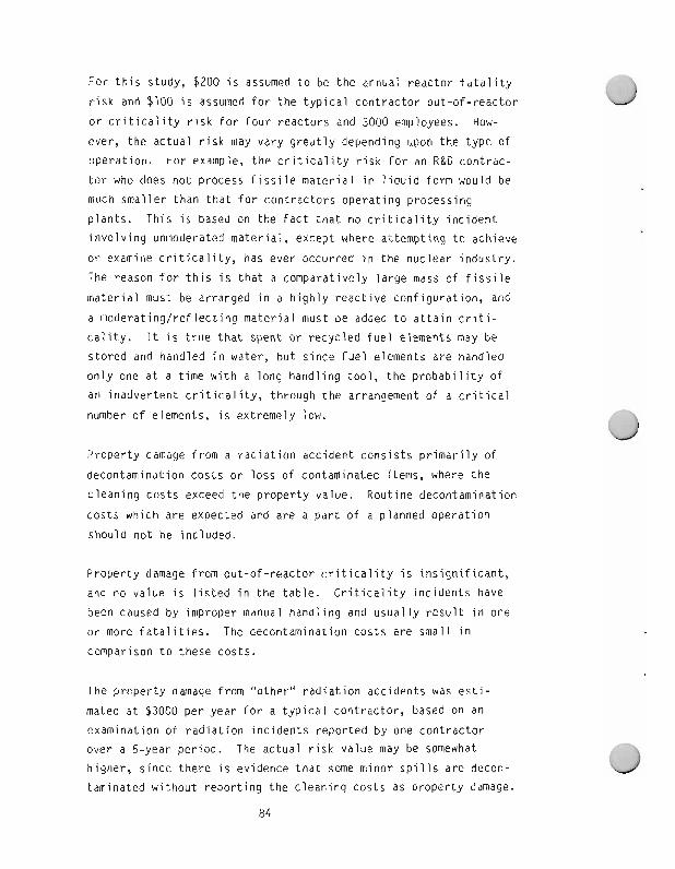
For this study, $200 is assumed to be the annual reactor fatality

risk and $100 is assumed for the typical contractor out-of-reactor

or criticality risk for four reactors and 3000 employees. How-

ever, the actual risk may vary greatly depending upon the type of

operation. For example, the criticality risk for an R&D contrac-

tor who does not process fissile material in liquid form would be

much smaller than that for contractors operating processing

plants. This is based on the fact that no criticality incident

involving unmoderated material, except where attempting to achieve

or examine criticality, has ever occurred in the nuclear industry.

The reason for this is that a comparatively large mass of fissile

material must be arranged in a highly reactive configuration, and

a moderatinglreflecting material must be added to attain criti-

cality. It is true that spent or recycled fuel elements may be

stored and handled in water, but since fuel elements are handled

only one at a time with a long handling tool, the probability of

an inadvertent criticality, through the arrangement of a critical

number of elements, is extremely low.

Property damage from a radiation accident consists primarily of

decontamination costs or loss of contaminated items, where the

cleaning costs exceed the property value. Routine decontamination

costs which are expected and are a part of a planned operation

should not be included.

Property damage from out-of-reactor criticality is insignificant,

and no value is listed in the table. Criticality incidents have

been caused by improper manual handling and usually result in one

or more fatalities. The decontamination costs are small in

comparison to these costs.

The property damage from "other" radiation accidents was esti-

mated at $3000 per year for a typical contractor, based on an

examination of radiation incidents reported by one contractor

over a 5-year period. The actual risk value may be somewhat

higher, since there is evidence that some minor spills are decon-

taminated without reporting the cleaning costs as property damage.

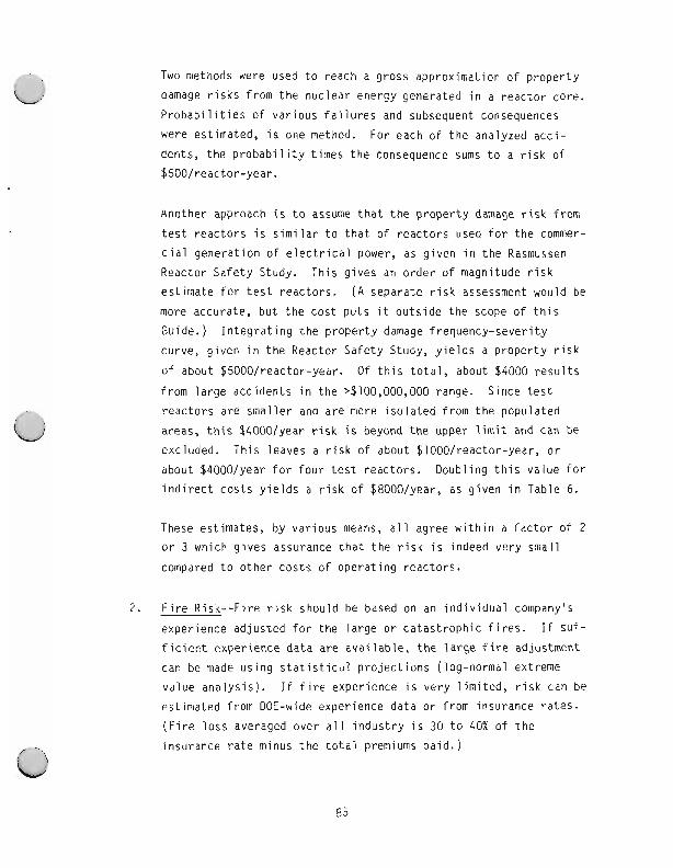
Two methods were used to reach a gross approximation of property

damage risks from the nuclear energy generated in a reactor core.

Probabilities of various failures and subsequent consequences

were estimated, is one method. For each of the analyzed acci- dents, the probability times the consequence sums to a risk of

$5OOlreactor-year.

Another approach is to assume that the property damage risk f r m

test reactors is similar to that of reactors used for the commer-

cial generation of electrical power, as given in the Rasrnussen

Reactor Safety Study. This gives an order of magnitude risk estimate for test reactors. ( A separate risk assessment would be

more accurate, but the cost puts it outside the scope of this

Guide.) Integrating the property damage frequency-severity curve, given in the Reactor Safety Study, yields a property risk

of about $5000/reactor-year. Of this total, about $4000 results

from large accidents in the ~$100,000,000 range. Since test

reactors are smaller and are more isolated from the populated

areas, this $4000/year risk is beyond the upper limit and can be

excluded. This leaves a risk of about $1000/reactor-year, or

about 340001year for four test reactors. Doubling this value for

indirect costs yields a risk of $8000/year, as given in Table 6.

These estimates, by various means, all agree within a factor of 2 or 3 which gives assurance that the risk is indeed very small

compared to other costs of operating reactors.

2. Fire Risk--Fire risk should be based on an individual company's

experience adjusted for the large or catastrophic fires. If suf-

ficient experience data are available, the large fire adjustment

can be made using statistical projections (log-normal extreme

value analysis). If fire experience is very limited, risk can be

estimated from DOE-wide experience data or from insurance rates.

(Fire loss averaged over all industry is 30 to 40% of the

insurance rate minus the total premiums paid.)

The AEC (DOE) 28-year cumulative fire 1085 ratio (1947 to 1974)

was 1.76 per $100 property valuation. l7 Without the Rocky

Flats fire, the ratio would have been less than a third of this

value. In the 5 years after the Rocky Flats fire (1970 to 19751,

the ERDA-wide fire loss ratio has been 0.093t per $100 value (if adjusted for catastrophic loss, the loss rate would undoubtedly

be higher). However, improvement is evident from the chart given

on Page 19 of WASH-1192,17 and probably results from extensive

fire protection improvements and increased concern for fire loss.

There is, however, statistical evidence that the fire loss ratio

has been increasing since the Rocky Flats fire, indicating a

possible decreasing concern as time passes. In addition, the

fire loss ratio is variable, being considerably higher at some

sites than others. Contractor risk estimates can be made from

local, DOE, or national experience, making adjustments as

appropriate.

3. Toxic Pathoqenic--Except for massive or serious acute exposures,

losses from toxic, carcinogenic, or pathogenic effects usually

are not identified. Since many months, or even years, may pass

prior to the onset of serious effects, an illness or injury

caused by exposure to toxic materials may never be related to

specific exposure incidents. In addition, the toxicity of many

substances has not been recognized because of the long, latent

periods before biological damage appears.

Of the 120 AEC occupational fatalities from 1959 through 1975,

one was caused by solvent vapors and three by asphyxiation in

confined spaces or inert atmospheres. Assigning asphyxiation to

the toxic category, 3.3% of the fatalities occur in this Cate-

gory. Although there are few toxic injuries, the injuryjdeath

risk is assumed to be the same for toxic materials as it is for

other energy categories. Thus, 3.3% of the total injuryjfatality

risk is assigned to toxicJpathogenic in Table 6.

4. Electrical Risk--Electrical risk includes hazards of downtime from

power failure, property damage from electric system failures, and

personnel i n j u r i e s f rom con tac t w i t h e l e c t r i c i t y . One shou ld be

cau t i ous n o t t o ove r l ook t h e l a r g e consequence p o t e n t i a l i n h e r e n t

i n e l e c t r i c a l systems. F a i l u r e s have p o t e n t i a l f o r l ong

downtimes and/or l a r g e f i r e s o r o t h e r p r o p e r t y damage. For

example, f o r e l e c t r i c p r o p e r t y damage r i s k Table 4 g i ves a va lue

t w i c e t h e average l o s s over a 5-year per iod .

I n a d d i t i o n , t h e i n j u r y r i s k may be h i g h even though few e l e c t r i c

shock i n j u r i e s have occurred. An e l e c t r i c i a n may n o t r e p o r t a

shock i f he i s n o t i n j u r e d , which under s l i g h t l y d i f f e r e n t

c i rcumstances may be f a t a l . To es t ima te t h i s f a t a l i t y r i s k ,

m u l t i p l y t h e number of i n j u r i e s by t h e c o n d i t i o n a l p r o b a b i l i t y o f

f a t a l i t y i f an i n j u r y occurs. An example i s g i ven below:

I n t h e p a s t 6 months, Company Z had 6 i n j u r i e s f rom e l e c t r i c a l

sources; 2 o f which were 600 v o l t s .

The f o l l o w i n g from "Acc ident Fac ts " shows d e r i v a t i o n of r e t u r n

p e r i o d and r i s k f o r e l e c t r i c f a t a l i t y :

S t a t i s t i c a l d a t a pub l i shed by t h e Na t i ona l Sa fe t y Counc i l i n

Acc ident Fac ts i n d i c a t e :

18.5% o f i n j u r i e s f rom L600 v o l t s a re f a t a l

1.6% of i n j u r i e s from <600 v o l t s a re f a t a l .

F a t a l i t y f requency f o r ,600 v o l t s :

f a t a l i t i e s 2/6 accidents/month x 0.185 injury

12 months = 0,74 f a t a l i t i e s X yea r yea r '

Fatality frequency for <boo volts:

accidents fatalities 4/6 month x 0.016 injury

x 12 months = 0,13 fatalities year year

All voltages = 0.74 + 0.13 = 0.87 .

1 Return period = frequency = 110.87 = 1.15 years .. Assuming $200,000 for a fatality, the annual risk is:

NOTE: This is an example and this risk value is not included in Table 6.

9. RISK ASSESSMENT OF NEW SYSTEMS

If a proposed facility and its operation involve no unique or unusual

hazards, the life cycle risk can be estimated from appropriate DOE-wide or

national property loss and injury incidence rates.

The following steps are necessary.

1. Divide the project into stages appropriate for risk estimation

such as:

a. Planning, design, and review

b. Construction

d. Decommissioning and dismantling.

2. Assess the routine risk in each stage by:

a. Determining the employee-hours and property values at risk

b. Multiplying the employee-hours and property values by

appropriate incidence rates; i.e., construction employee-

hours and property values times construction incidence rates

c. Considering any environmental or public effects for each

stage.

3. Assess the nonroutine risk in each stage by:

a. Considering the breakin period and training of new emplOYee8

during the first year. (Because personnel are unfamiliar

with procedures and equipment, mistakes are more likely.)

Data show that even experienced bus drivers have an increased

accident probability when assigned to a new route, and con-

sequently, first year employees have a higher injury rate.

In the absence of data, a factor of 2 or 3 over average accidents rates is suggested.

b. Consider the latter stages of plant life. Will risk increase

because of complacency and carelessness engendered by famil-

iarity? Will funds be provided to replace old equipment or

will recommended service life likely be exceeded? No guide- line is given here because the increased risk varies greatly

depending upon hazards associated with breakdown of aging

equipment and because data of a general nature are unavail-

able. However, the risk can increase enormously as equipment ages.

c. Screening energy sources at each stage and assessing the

risk for unusual hazards such as nuclear, vehicle (for

operations with large transportation needs), thermal (for

solar reflectors), etc.

4. Sum the various risks to obtain the total. While outside the

scope of this risk manual, risk assessment is only a part of an

adequate safety analysis report which should, among other things,

document the control procedures and safety staff assumed in the

risk assessment. There is ample evidence that a professional

safety staff and comprehensive review system will reduce risks by

factors of 5 to 10 over that of a project with only one safety

engineer for 5 to 10 thousand workers.

9.1 Resource Allocation

For optimum efficiency, the effort applied to risk control should be

consistent with the degree of magnitude of risk. The curve in Figure 7

pictures qualitatively the relationships between safety investment costs

and accident costs. As shown in Figure 7, safety investment is represented

by a straight line, while accident costs are represented by the decreasing

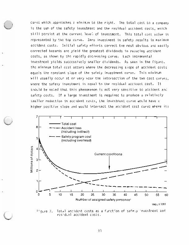
cu rve which approaches a minimum t o t h e r i g h t . The t o t a l c o s t t o a company

i s t h e sum of t h e sa fe t y investment and t h e r e s i d u a l acc ident cos ts , which

S t i l l p e r s i s t a t t h e c u r r e n t l e v e l of investment. Th i s t o t a l c o s t va lue i s

represented by t h e t o p curve. Zero investment i n s a f e t y r e s u l t s i n maximum

acc iden t cos ts . I n i t i a l sa fe t y e f f o r t s c o r r e c t t h e most obvious and e a s i l y

c o r r e c t e d hazards and y i e l d t h e g r e a t e s t d i v i dends i n reduc ing acc ident

cos ts , as shown by t h e r a p i d l y decreas ing curve. Each incrementa l

investment y i e l d s success i ve l y sma l l e r d i v i dends . As seen i n t h e f i g u r e ,

t h e minimum t o t a l c o s t occurs where t h e decreas ing s lope of acc iden t cos t s

equa ls t h e cons tan t s l ope of t h e sa fe t y investment curve. T h i s minimum

w i l l u s u a l l y occur a t o r ve ry near t h e i n t e r s e c t i o n o f t h e two c o s t curves,

where t h e s a f e t y investment i s equal t o t h e r e s i d u a l acc ident cos t . It

shou ld be noted t h a t t h i s phenomenon i s n o t v e r y s e n s i t i v e t o acc iden t and

sa fe t y cos ts . I f a l a r g e investment i s r e q u i r e d t o produce a r e l a t i v e l y

s m a l l e r r e d u c t i o n i n acc iden t cos ts , t h e investment curve would have a

h i g h e r p o s i t i v e s lope and would i n t e r s e c t t h e acc iden t c o s t cu rve where i t s

-0 5 10 15 20 25 30 35 40 45 50 55 60

Number of assigned safety personnel INEL23361

6

F i g u r e 7. T o t a l acc iden t cos t s as a f u n c t i o n of s a f e t y investment and r e s i d u a l acc iden t cos t s .

-'Total cost - ----Accident loss -

(including indirect)

- (including overhead)

-

Current conditions

1

\ 4-

- '-. I- -

/- --------____ "--I- I I I I I 1 I I I I

nega t i ve s l ope i s a l s o g rea te r . L ikewise, a low investment y i e l d i n g l a r g e

d i v i dends r e s u l t s i n an i n t e r s e c t i o n f a r t h e r t o t h e r i g h t where t h e acc iden t

c o s t cu rve i s a l s o r e l a t i v e l y f l a t .

Thus, i t i s reasonab ly c e r t a i n t h a t t o t a l c o s t s a re a t a minimum when

resources devoted t o sa fe t y a re about equal t o r e s i d u a l acc ident cos ts . I t

shou ld a l s o be noted t h a t t h e t o t a l c o s t cu rve i s r e l a t i v e l y f l a t over a

f a i r l y wide range of sa fe t y investment. T h i s means t h a t a company can

i n v e s t resources i n sa fe t y t h a t a re s i g n i f i c a n t l y l a r g e r t han t h e r e s i d u a l

acc iden t cos t s w i t h l i t t l e t o t a l increased cos t . I t a l s o means t h a t gross

es t ima tes a re o f t e n adequate t o determine whether i n s u f f i c i e n t o r excess

resources a re be ing i nves ted i n safety.

The a c t u a l d o l l a r va lues g i ven i n F i g u r e 7 were de r i ved as f o l l o w s .

The sa fe t y program cos ts were based on a c o s t of $40,000 p e r p ro fess iona l

Safety eng ineer o r r a d i o l o g i c a l engineer. (The 140,000 i nc ludes a l l over -

head expenses and i n d i r e c t personnel s a l a r i e s averaged over 33 d i r e c t s a f e t y

personne l . ) The acc iden t l o s s cu rve was approximated f rom o n l y one f i r m

p o i n t : t h e c u r r e n t acc iden t l o s s o f $500,000 g i v e n i n F i g u r e 7, and t h e

c u r r e n t number of 33 sa fe t y p r o f e s s i o n a l s assigned t o o p e r a t i o n a l a c t i v i t i e s

f o r a t y p i c a l c o n t r a c t o r . S ince t h e average s e v e r i t y , f requency, i n j u r y ,

and v e h i c l e acc iden t r a t e s g i ven by t h e Na t i ona l S a f e t y Counc i l range from

5 t o 15 t imes g r e a t e r t han a t y p i c a l DOE c o n t r a c t o r , i t was assumed t h a t if

t h e company had o n l y one i n s t e a d of t h r e e sa fe t y engineers, t h e r e s i d u a l

r i s k o f acc iden t losses would be 10 t imes as h i g h ( o r f i v e m i l l i o n d o l l a r s

p e r yea r ) . T h i s g i v e s a second p o i n t : one eng ineer versus f i v e m i l l i o n

d o l l a r s . An approx imat ion o f t h e s l ope of t h e acc iden t c o s t cu rve a t t h e

c u r r e n t l e v e l of 33 eng ineers was ob ta ined from a hazard s e n s i t i v i t y

study. The consensus g i ven i n t h e De lph i s tudy (d iscussed l a t e r i n t h i s

s e c t i o n ) i s t h a t a t t h e c u r r e n t l e v e l of sa fe t y s ta f f i ng , t h e a d d i t i o n o r

d e l e t i o n of one man would e v e n t u a l l y change t h e r i s k by about $10,00O/year.

Since two p o i n t s and t h e s lope a t one p o i n t a re known and t h e cu rve i s

approx imate ly exponen t i a l , t h e complete cu rve can be drawn w i t h reasonable

accuracy. By exponen t i a l we mean t h a t t h e f i r s t person c o r r e c t s t h e

e a s i e s t most obvious hazards, and t h e second person c o r r e c t s i tems t h e

f i r s t person missed. W i th succeeding persons, we reach a p o i n t of

d i m i n i s h i n g re tu rns ; thus , s l ope i s s teeper a t f i r s t and f l a t t e n s

out . I t i s b e l i e v e d t h a t t h e cu rve i s accura te w i t h i n a f a c t o r o f 2 on t h e

l e f t , w i t h t h e accuracy i nc reas ing t o about 20% i n t h e range of 20 t o

40 sa fe t y personnel .

It i s i m p r a c t i c a l t o c o n s t r u c t a s i m i l a r resource acc iden t c o s t cu rve

f o r each energy type. However, it i s obvious t h a t t o t a l r i s k c o n t r o l

resources a re a l l o c a t e d a t optimum e f f i c i e n c y if t h e resources and s p e c i f i c

energy r e s i d u a l r i s k s a re r e l a t i v e l y un i fo rm, r a t h e r t han l a r g e sums be ing

spent on smal l r i s k s , and v i c e versa.

To measure t h e degree of balance o r u n i f o r m i t y i n a s a f e t y program,

determine t h e percentage o f resources spent on each t ype of r i s k and d i v i d e

by t h e degree of r i s k . As an i l l u s t r a t i o n , t h i s exe rc i se f o r a c o n t r a c t o r

f o l l ows .

The annual resources i n man-years a l l o c a t e d t o each r i s k i n Tab le 8

were determined. Some o f t h e ca tego r i es g i ven i n Tab le 8, such as c r i t i -

c a l i t y and f i r e , were e a s i l y and a c c u r a t e l y es t imated. Others, such as

c o r r o s i v e and thermal, a re o n l y educated guesses. The es t ima tes can be

g r e a t l y improved i f s a f e t y p ro fess iona l s work ing i n mu l t i ene rgy c a t e g o r i e s

keep a l o g of t h e i r t ime spent i n each category . The l o g needs t o be k e p t

o n l y l o n g enough t o e s t a b l i s h t h e d i v i s i o n of t i m e and a t p e r i o d i c i n t e r -

v a l s t o mon i to r changes. A t a b l e s i m i l a r t o Table 8 can then be con-

s t ruc ted . Loca l d e c i s i o n s must be made rega rd ing which personne l shou ld

l o g i c a l l y be i nc luded i n t h e s a f e t y manpower a l l o c a t i o n . N o t i c e a b l y absent

i n Tab le 8, f o r example, a re s a l a r i e s and o t h e r c o s t s f o r t h e f i r e depa r t -

ment which i s DOE-operated, r a t h e r t han cont rac tor -opera ted, a t t h i s

p a r t i c u l a r l o c a t i o n .

Assuming t h e man-years spent on each ca tego ry a re p r o p o r t i o n a l t o t h e

s a f e t y program c o s t s f o r each category, resource percentages were c a l c u l a t e d

d i r e c t l y f rom t h e man-years.

There are, no doubt many ways t o es t ima te resources a l l o c a t e d t o

sa fe t y . T o t a l s a l a r i e s and overhead cos ts c o u l d be used b u t these a re

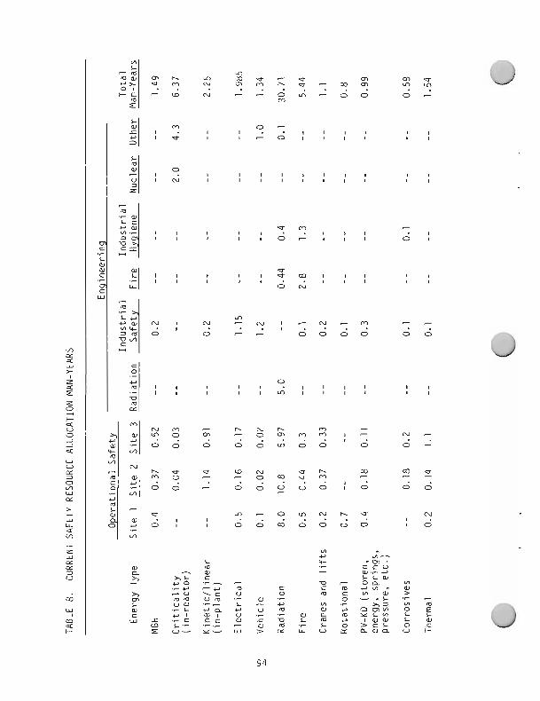
in ir

5 >

2 r z 0 C

5 0 .-I

N 7 . . 2 m

*- v, 0 O O L " O 0 0 0 -

w 0

v,

LZ 3

* F. m m cf 0

- 7

in . .

w 0 . 7 0 0 - O O _ O O O I 0 0 0

LZ C

> + w

L " 7 ? " " " " . . . . N

". , . 4

0 0 m 0 0 o o I 0

v,

m L - m

m r

L" m w m L" m e - * m g y - 7 N m m h e - m m

m e . . . . . . . L" L"

+ = - a N - - o L " - o o . . m

0 7

0 9 - , , , , 1 - 0 1 1 8 1

8 0 8 8

b I I I , , , 4 I I I 1 1 1

I I I ,

e m 7

4 I . . I , , l , O - , , , . 8

0 8

cf I a * m r 8 I I t . . , , ,

I I

0 N 8 L

L" N N , N i m . . , . . . . 7 7

a 7 -

. . 0 0 0 0 0 0

c m .r

C

.- m m z

O l I I I , , ? , , , , 1 1 m 1 1 1 ,

I I I I

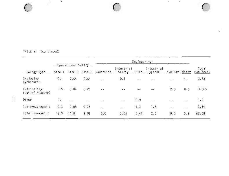
TABLE 8. (continued)

Operational Safety

Energy Type

Explosive 0.1 pyrophoric

Criticality 0.5 (out-of-reactor)

a " Other 0.1

Toxicfpathogenic 0.3

Total man-years 12.0

Site 2

0.04

Site 3

0.04

Industrial Radiation Safety

Industrial Total Fire Hyqiene Nuclear Other Man-Years -

reasonably proportional to the manpower spent in the field. Costs which may not be proportional are personnel safety equipment and increased capital

equipment and operational costs required to meet safety requirements.

Specific costlbenefit analysis is often more appropriate than generali-

zation of these items as safety investments. The cost of meeting minimum codes and standards should be included only in cost/benefit analyses during

evaluation of proposed standards, but not in overall safety investment/

accident cost trade-off studies.

The percentage of risk for each energy category (calcualted from risks

in Table 81, the resource percentage and the resource to risk rates are

calculated and tabulated as in Table 9. The percentage resource divided by

the percentage risk gives a ratio that is indicative of the relative safety

resource/risk relationship. A ratio of <1 means that less than average

attention is being given to safety, and a ratio >l means more than average

attention to safety. These ratios are given for total risks (including

intangible effects) and company risks only (tangible direct and indirect

losses). In Table 9, the energy types are listed, with those receiving the

least relative attention at the top and those receiving more at the bottom.

The total resource/risk comparison is also given in bargraph form in

Figure 8. The multiplier of 10 applied to nuclear risks (included in the

bargraph) changes these ratios significantly. The total risk ratios are the

ones of direct interest, since implicit in the multiplier of 10 is that it

is worthwhile to spend 10 times as much to prevent a nuclear accident, as to prevent a nonnuclear incident having the same direct dollar loss.

There are no data available from which to determine directly the

sensitivity of the residual risk level to changes in the level of safety

effort allocated to each energy type; however, an approximation can be

obtained from opinions of safety specialists. One method of obtaining a

consensus is a Delphi study. This technique permits interchange of thought

without the study participants meeting as a group. The steps in a Delphi

study are as follows:

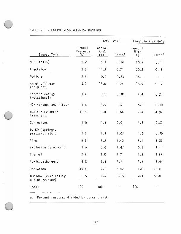
TABLE 9. RELATIVE RESOURCE/RISK RANKING

Energy Type

MGH (falls)

Electrical

Vehicle

Kineticllinear (in-plant)

Kinetic energy (rotational)

MGH (cranes and lifts)

Nuclear (reactor transient)

Corrosives

PV-KD (springs, pressure, etc.)

Fire

Explosive pyrophoric

Thermal

Toxic/pathogenic

Radiation

Nuclear (criticality out-of-reactor)

Total

Annual Resource

( % I

2.2

3.2

2.5

3.2

1.2

1.6

11.8

1.0

1.5

9.5

1.0

2.2

6.2

45.6

5.5

100

Total Risk Tangible Risk Only

Annual Risk 0 15.1

14.8

10.9

13.5

3.2

3.9

18.0

1.1

1.4

6.8

0.6

1.0

2.3

7.1

0.4

100

Annual Risk L 20.7

20.2

15.0

18.5

4.4

5.3

2.4

1.5

1.9

5.1

0.9

1.3

1.8

1.0

0.1

100

a. Percent resource divided by percent risk.

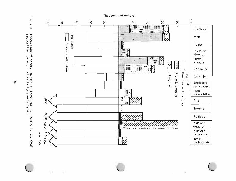
Thousands of dollars

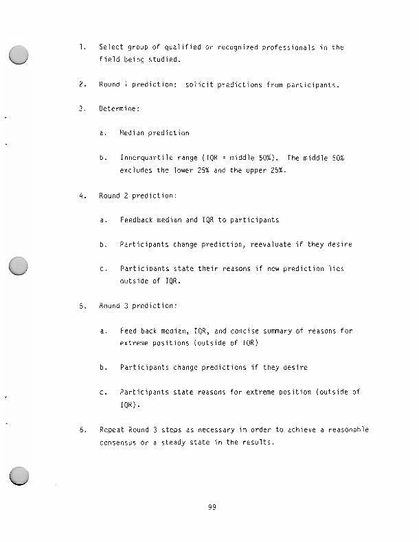
1. Select group of qualified or recognized professionals in the field being studied.

2. Round 1 prediction: solicit predictions from participants.

3. Determine:

a. Median Drediction

b. Innerquartile range (IQR = middle 50%). The middle 50%

excludes the lower 25% and the upper 25%.

4. Round 2 Drediction:

a. Feedback median and IQR to participants

b. Participants change prediction, reevaluate if they desire

C. Participants state their reasons if new prediction lies

outside of IQR.

5. Round 3 prediction:

a. Feed back median, IQR, and concise summary of reasons for extreme positions (outside of IQR)

b. Participants change predictions if they desire

c. Participants state reasons for extreme position (outside of

IQR).

6. Repeat Round 3 steps as necessary in order to achieve a reasonable

consensus or a steady state in the results.

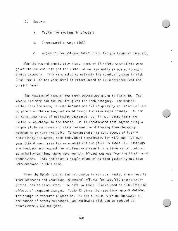
7. Report:

a. Median (or medians if bimodal)

b. Innerquartile range ( I Q R )

c. Arguments for extreme position (or two positions if bimodal).

For the hazard sensitivity study, each of 12 safety specialists were

given the current risk and the number of men currently allocated to each

energy category. They were asked to estimate the eventual change in risk

level for a 112 man-year level of effort added to or subtracted from the

current level.

The results of each of the three rounds are given in Table 10. The median estimate and the IqK are given for each category. The median,

rather than the mean, is used because one "wild" guess by an individual has no effect on the median, but could change the mean significantly. As can be seen, the range of estimates decreased, but in most cases there was

little or no change in the median. It is recommended that anyone doing a

Delphi study ask those who state reasons for differing from the group

opinion to be very explicit. To demonstrate the consistency of hazard sensitivity estimates, each individual's estimates for +I12 and -112 man-

year (third round results) were added and are given in Table 11. Although

the feedback and request for explanations result in a tendency to conform

to majority opinion, there were not significant changes from the first round

predictions. This indicates a single round of opinion gathering may have

been adequate in this case.

From the Delphi study, the net change in residual risks, which results

from increases and decreases in control efforts for specific energy cate-

gories, can be calculated. The data in Table 10 were used to calculate the

effects of proposed changes. Table 12 gives the resulting recommendations

for change in resource allocation. As can be seen, with no increases in the number of safety personnel, the estimated risk can be reduced by

approximately 138,000lyear.

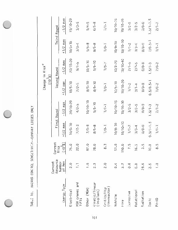
w n C

L

a m 0,

7 "7 - C -7 ( C 0 m w Z Z Z . - * 7

U T 7 " W a c

.- m - u a m m w 5 8 0

L L . U W 7 .' 0 .-

C urn I C a .?L U rn . Y 0 u w w , C , . L 2 . Y e

W w I- II C T . II - o . - i . . - L - a , . L Y g Z 2: W r - O V - U - > ~ U w ~ C a

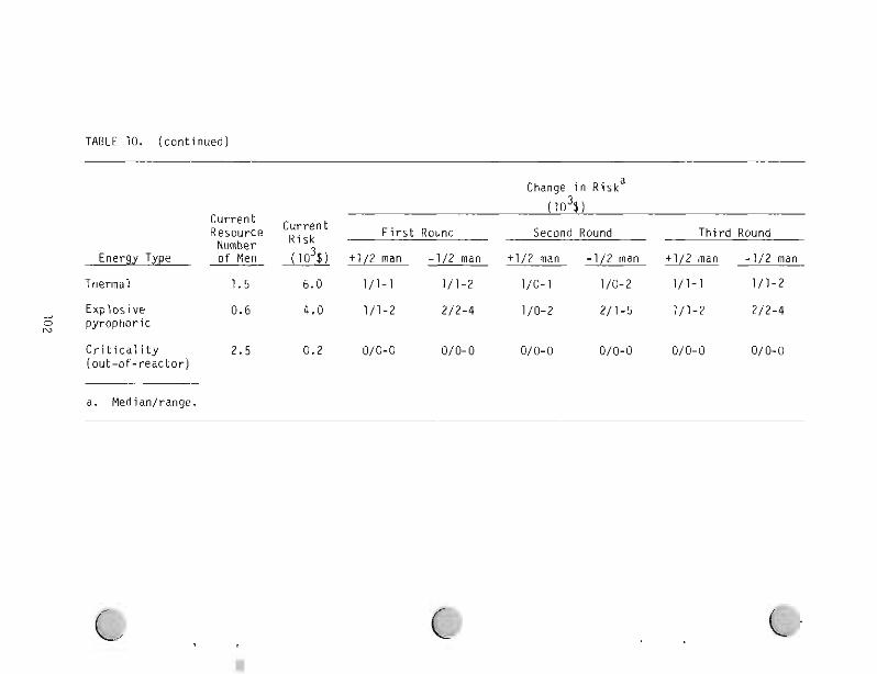
TABLE 10. ( c o n t i n u e d )

Change i n t? iska

C u r r e n t ( l o 3 $ )

C u r r e n t Resource Risk F i r s t Round Second Round T h i r d Round Number

Energy Type of Men (1031) +1/2 man -1/2 man +1/2 man -1/2 man +1/2 man - l / 2 man

Thermal 1.5 6 .0 1/1-1 1 /1-2 1/0-1 1/0-2 1/1-1 1/1-2

E x p l o s i v e 0.6 4.0 1 /1-2 2 /2-4 1/0-2 2/1-5 1/1-2 2/2-4 p y r o p h o r i c

C r i t i c a l i t y 2.5 0.2 O/O-0 O/O-0 O/O-0 O/O-0 O/O-0 O/O-0 ( o u t - o f - r e a c t o r )

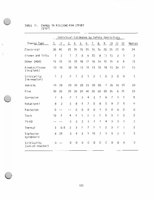
TABLE 11. CHANGE IN RISK/ONE-MAN EFFORl ($lo3)

Individual Estimates by Safety Specialists

1 2 3 4 5 6 7 8 9 1011xl2 Energy Type - - - - - - - - - - - Electrical 30 45 25 35 15 25 10 15 20 25 23 15 24

Cranesand lifts 7 2 7 7 8 6 20 8 13 15 3 3 7

Other (MGH) 15 15 15 18 18 17 18 14 15 15 0 8 15

Kinetic/linear 13 10 10 16 13 15 13 10 18 15 24 11 13 (in-plant)

Criticality 1 2 2 1 2 1 2 1 0 3 0 0 1 (in-reactor)

Vehicle 15 20 20 35 20 23 20 20 7 30 15 25 20

Fire 30 20 25 30 20 40 20 20 20 35 6 35 23

Corrosive 7 6 2 7 3 4 3 7 6 7 3 2 5

Rotational 8 3 5 8 4 7 5 8 5 9 7 5 6

Radiation 0 -- - - 0 0 0 0 1 0 0 0 0 0

Toxic 1 0 2 4 4 1 2 2 2 5 3 1 2 2

PV-KD -- .- 3 3 3 3 3 1 4 3 3 1 3

Thermal 3 0 . 5 2 3 2 7 2 1 2 3 2 1 2

Explosive 6 2 5 3 4 5 5 1 0 7 5 5 3 1 5 pyrophoric

Criticality 0 - - 0 0 0 0 0 0 0 0 0 0 0 (out-of-reactor)

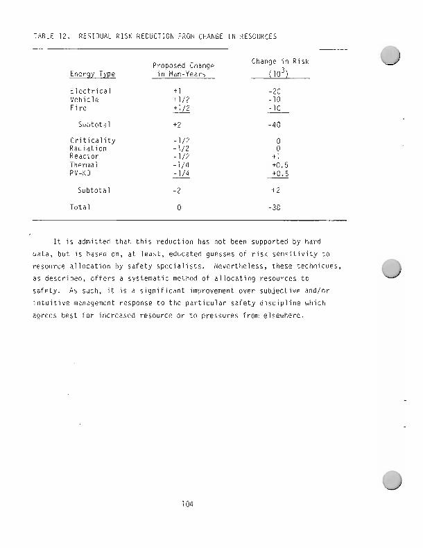
TABLE 12. RESIDUAL RISK REDUCTION FROM CHANGE IN RESOURCES

Proposed Change Change in Risk

Enerqy Type in Man-Years (lo3)

Electrical t 1 Vehicle +I12 Fire +1/2 - Subtotal +2 -40

Criticality -112 Radiation -112 Reactor -112 Thermal -114 PV-KO -114 - Subtotai - 2

Total 0 -38

It is admitted that this reduction has not been supported by hard

data, but is based on, at least, educated guesses of risk sensitivity to

resource allocation by safety specialists. Nevertheless, these techniques,

as described, offers a systematic method of allocating resources to

safety. As such, it is a significant improvement over subjective and/or

intuitive management response to the particular safety discipline which

agrees best for increased resource or to pressures from elsewhere.

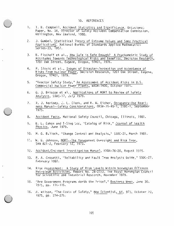
10. REFERENCES

I. B. Campbell, Acc ident S t a t i s t i c s and S ign i f i cance , Occasional Paper, No. 34, D i r e c t o r of Safety Acc ident Compensation Commission, Wel l ing ton, New Zealand, 1980.

J. Gumbel, S t a t i s t i c a l Theory of Extreme Values and Some P r a c t i c a l App l i ca t i ons , N a t i o n a l Bureau of Standards App l i ed Mathematics Ser ies-33, 1957.

B. F i s c h o f f e t al., How Safe i s Safe Enough? A Psychometr ic Study of A t t i t u d e s Towards Techno log ica l R i sks and Benef i ts , Dec i s i on Research, 1201 Oak S t ree t , Eugene, Oregon, 97401, 1976.

P. S l o v i c e t al., Images of D i sas te r -Pe rcep t i on and Acce tance o f R i s k s From Nuc lear Power, Dec i s i on Research, 1201 Oak StFeet, Eugene, Oregon, 97401, 1979.

"Reactor Safe ty Study," An Assessment of Acc ident R i sks i n U.S. Commercial Nuc lear Power P lants , WASH-1400, October 1975.

G. J. B r i scoe e t al., A p p l i c a t i o n s of MORT t o Review of Safe ty Ana lys is , SSDC-17, J u l y 1979.

R . J. Nertney, J. L. C lark , and R. W. E icher , Occupancy-Use Readi- ness Manual--Safety Cons idera t ions , ERDA-76-45-1, SSDC-1, September 1975.

Acc ident Facts, N a t i o n a l Safe ty Counci l , Chicago, I l l i n o i s , 1981.

8 . L. Cahen and I -S ing Lee, "Cata log of Risk," Journa l of H e a l t h Physics, June 1979.

M. G. Bu l l ock , "Change Con t ro l and Ana lys is , " SSDC-21, March 1981.

W. G. Johnson, MORT--The Manaqement Ove rs igh t and R isk Tree, SAN 821-2, February 12, 1973.

A c c i d e n U I n c i d e n t I n v e s t i g a t i o n Manual, ERDA-76-20, August 1975.

P. A. C r o s e t t i , " R e l i a b i l i t y and F a u l t Tree A n a l y s i s Guide," SSDC-22, February 1982.

R i s k Assessment: A Study of R i sk Leve ls W i t h i n Norwegian Offshore Petroleum A c t i v i t i e s , Report No. 26-27/2, The Royal Norwegian Counc i l f o r S c i e n t i f i c and I n d u s t r i a l Research, November 1979.

"Are Government Programs Worth t h e Pr ice?, " Business Week, June 30, 1975, pp. 114-115.

R. Wilson, "The Costs of Safety," New S c i e n t i s t , 68, 973, October 20, 1975, pp. 274-275.

17. O p e r a t i o n a l Acc i den t s and R a d i a t i o n Exposure Exper ience 1943-1975, WASH-1192, 1975.

18. "On t h e E v a l u a t i o n of Human L i f e i n Acc i den t S tud ies , " Acc i den t A n a l y s i s and Prevent ion , Pergamon Press, 5, 1973, pp. 287-293.

N. W. Knox and R. W. E icher , MORT U s e r ' s Manual, ERDA-76-45-4, SSDC-4, Narch 1976.

F a u l t Tree f o r Safe ty , Support Systems Engineer ing, Boeing M i l t a r y A i r c r a f t Product Development, November 1968.

W. D. Rowe, D r a f t , An Anatomy of Risk, Environmental P r o t e c t i o n Agency, March 1975.

0 . L. Cohen and I - L i n g Lee, "Cata log o f Risks," Journa l o f Hea l t h Physics, June 1979.

APPENDIX A RISK IDENTIFICATION TREE

APPENDIX A

RISK IDENTIFICATION TREE

A logic structure in the form of risk identification tree can be used

to make a thorough search for all hazards. It will minimize the number of

hazards which may otherwise be overlooked.

Block 1.0 of the Risk Identification Tree defines the objective, i.e.,

bringing to the attention of management the "Residual Operational Risks"

remaining after the risk analysis has been completed, and corrective action

has been taken to eliminate and control major risks. Subordinate blocks

(1.0 through 5.0) define the necessary and sufficient conditions to achieve

fulfillment of the objective stated in Block 1.0. These conditions are:

1. All energy sources must be identified

2. All potential targets of uncontrolled energy release must be

identified for each enerqy source

3. All control mechanisms and barriers to energy release must be

identified for each energy source

4. An analysis must be performed in each case to determine failure

modes and effects, in order to identify the residual risks.

The balance of the tree provides a guide for identifying all energy

sources. The two lower tiers on Page A-4 identify the various forms of

energy. The transfer symbols relate to tabulations on Pages A-5 through 12

of specific risk situations. The tabulations are general in nature, but

are traceable to specific hardware, locations, and organizational units.

Identifying of all energy sources and tracing them to specific hardware

has the primary benefit of preventing oversight of specific hazards. The

safety analyses associated with Conditions 2, 3, and 4, above, are time- consuming. Therefore, the high risk energy sources should be considered

first and the analytical effort scaled to the degree of risk. The selection

and scaling should be made by safety specialists. Although the selection of high risk hazards does not quantify the risk, it will help to prevent

oversight of high risk areas.

The tree provides a logical sequence for a structured search of

hazards which include the following steps:

1. Identify each energy source. An energy source is any material or condition which could result in a release of energy. Examples are combustibles, toxic substances, corrosive materials, electric

or radient energy, moving objects or machinery and objects which

could fall or drop. A list of energy types are given in Table 6

in the main text. A list with many examples are given in the

Safety Analysis Guide SSDC.

2. Identify all potential targets of uncontrolled energy release for

each energy source equipment, facilities, employers, public, and

environment should all be considered.

3. Identify all control mechanisms and procedures for each energy

source and target. These include time, space, and physical

guards or barriers.

4. Perform an analysis to determine failure modes and effects to

identify the residua1 risks. (This only identifies the risks;

probability estimates are necessary to quantify the risk.)

An understanding of this method will alert a person to hazards in

making plant inspections or in just walking through the plant even though a

structured search is not conducted. A thorough search using the tree will minimize hazard oversight. Since the procedure is time consuming, high

energy sources could be considered (Steps 2, 3, and 4) first.

RISK IOENTIFICATION TREE

TYPICAL LOWER T I E 9 STRIJCTURE

a.1.1 r----------1 ! E l e c t r i c a l :

l"J"& - Field Mon i to r ing Program

S t a t i s t i c a l Data Stores

Reported S ign i f i can t Observation Studies

Area Safety Manager Reports

F i r e Safety and Operation Condi t ions Study

P r i o r i t y Problem L i s t s

RDT inc iden t Reports

OSHA i n r p e c t i a n r

Design Studies and Analyses

Safety Enqineer L i s t s

A. 1

Sources D i ~ t r i b u t i o n

B a t t e r y Bankr T ~ d n s f o m e r ~ Pumps D l e r e l Un i t s Wir ing High L i n e r

Motors Switchgear Heaters Underground Wnrins Power TOOIS Cable R u m h a l l Equ ip len t Serv ice Out le ts

and F i t t i n q s

TYPICAL LOWER T I E R STRllCTURE

(ENERGY SOURCES GEOGRAPHICALLY MOBILE)

a.l.2 ,------------ I Nuclear I 1.. . - - . - p.a3

4 I 8 1

Storage

vaults Temporary Storage Arear Receiying Arear Shipping Arear Casks Burial G I O U " ~ ~ Storwe Rackr Canals and Barinr Reactor lo-Tank Storage

Dollies Trucks Hand Carry c p m e s Lifts Comerclal

fl Modification ,Jq Redcto~s C~itical Facilities Subcritical A s s ~ b l i e r

lnrpectian Areas Ldbo~ato~les Test Risr Pllot Plants

I C.2 f a l l i n q Object

Darnaged P 1 do llunan E f f o r t L i f t s P i t s

C P ~ B I . Jacks, L i f t s Cranes E x ~ w a t i o n s Bucket and Ladder E l e v a t e d DOOPI Trucks Canals S l i n g s Vessels H o i s t s E l e v a t o r s Jacks Scsffolda and Ladders Crane Cabs

i I PY and KO I L--__ _ _ _ _ J

p. i i -2 4 Thermally A c t i v a t e d A c t i v a t e d

B a i l e r r Gas B o t t l e r Heated Surge T a n k P?es%re Vessels Autoclaves C o i l e d Springs Test Loapr and F a c i l i t i e s Stressed Members

Gas Receivers

E. l

Vehicular

I

I E.1.1 Highway In-House Vehicles Vehicles Rai 1 road Personnel Equipment

Cars Fork L i f t s Rai 1 road Surfaces Shears Trucks Carts Obstructions Presses Buses Do1 1 i e s Crane Loads i n Motion

PV Blowdown Power Assisted D r i v i n g Tools

a.2.2 r----------I ' Rota t iona l 1 L ---- ----,

p.A-2 A Centr i fuges Motors Pumps Cool ing Tower Fans Cafe te r ia Equipment Laundry Equipment Gears Shop Equipment (Grinders,

Saws, Brushes, e tc . ) F l o o r Po l i shers

a.3.1 r----------0 I I I Corros ive I

p.A-2

Acids Caust ics "Natura l " Chemicals

( S o i l . A i r . Water)

a.3.3 r---------I 1 Toxic I

p.A-2

Caps Acetone Primer Cord F lour ides Dynamite Co Powder Meta l lu rgy Lead Dusts h o n i a Hydrogen ( I n c l . B a t t e r y Asbestos

Banks and Water Decomp.) T r i ch lo roe thy lene Gases - Other Dusts and P a r t i c u l a t e s Gd N i t r a t e Pes t i c ides - Herb ic ides E l e c t r i c Squibbs I n s e c t i c i d e s Peroxides - Superoxides Bac te r ia

Be Ch lo r ine Decon So lu t ions Sandblast Metal P l a t i n g Asphyxiat ion - Drowning

Packing M a t e r i a l Raas ~ a Z o l i n e (Storage and i n Veh ic les ) Lube O i l Coolant O i l P a i n t So lven t D iese l Fuel B u i l d i n g s and Contents T r a i l e r s and Contents Grease Hydrogen ( I n c l . B a t t e r y Banks) Gases - Other Spray P a i n t So lven t Vats

i Thermal i I (Except Radiant) I Enerov I

Convection Heavy Metal Weld Preheat Exposed Steam Piper E l e c t ~ i c Heaters F i r e Boxer Lead Mel t Pat E l e c t r i c a l Wi r ing and Equipment

d _ Furnaces

and ~ e a c t b r Equip.

a 5 . 1 r-----------.

1 . 1 I L. I 1.3 L.4

- - E l e c t r i c Furnace BldCXl ight (e .g . , M a g n i f l u x ) Laser Medical K-Ray Radiography Equipment Welding E l e c t r i c Arc - Other (High

Current CKTS) E lec t ron Beam

Storage T r a n s p o r t d t i m Mod i f i ca t ion Fabr i ca t ion

Canals " S ~ U ~ C ~ S " Inspec t ion

A p p l i c a t i o n and Use

"Sourcer" Plug Storage Waste and Scrap " S O U T C ~ S " Warte and scrap S t o ~ a g e Areas Contamination uar te and scrap COntarninatian Storage Bu i ld ings I r r a d . Experimental contamination I r r a d . Experimental

and Reactor Equip. Exoerimenta, and Reactor Equip.

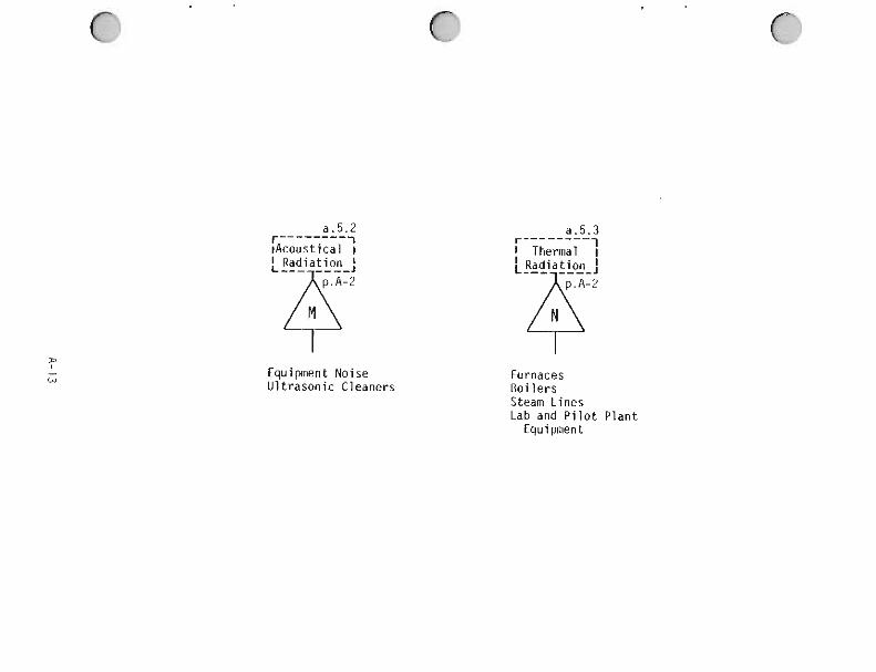
Equipment Noise U l t rason ic Cleaners

Furnaces Bo i le rs - -

Steam Lines Lab and P i l o t P lan t

Equipment

APPENDIX B

USE OF RISK PROJECTION TECHNIQUES

IN INVESTIGATION OF ACCIDENTS AND INCIDENTS

APPENDIX B USE OF RISK PROJECTION TECHNIQUES

I N INVESTIGATION OF ACCIDENTS AND INCIDENTS

1. I n t r o d u c t i o n

An impor tant f a c t o r i n i n v e s t i g a t i o n of acc iden ts o r i n c i d e n t s i s t h a t

o f r e l a t i n g t h e acc ident o r i n c i d e n t under i n v e s t i g a t i o n t o normal behav ior

o r t h e o r g a n i z a t i o n expe r i enc ing t h e event.

" I t em f i x e s " ( remedia l a c t i o n s based on t h e s p e c i f i c s of t h e acc iden t )

a n d "system f i x e s " ( remedia l a c t i o n s having t o do w i t h t h e o v e r a l l c o n t r o l

Fystprn w i t h i n which t h e acc ident o r i n c i d e n t occur red) fo rm an e s s e n t i a l

l i a r t o f r e a c t i o n t o any acc iden t o r i n c i d e n t . I n o rde r t o frame e f f e c t i v e

vemedial recommendations, i t i s , however, necessary t o understand t h e degree

Lo which t h e acc iden t i s t y p i c a l o f o r g a n i z a t i o n a l behav ior . When r e l a t e d

o r g a n i z a t i o n a l o p e r a t i n g exper ience e x i s t s , t h e r e are two s t a t i s t i c a l

rm~thods f o r r e l a t i n g t h e consequences of a severe acc iden t t o normal o rgan i -

l i t i o n a l behav ior . The f i r s t method i n v o l v e s s tudy of pas t f requency-

cpveri1.y da ta and d e r i v a t i o n o f t h e p r o b a b i l i t y (expected f requency) o f t h e

pverlt under study. The second method makes use of o n l y t h e more s e r i o u s

Pven ls ~ x p e r i e n c e d i n t h e p a s t t o d e r i v e t h e l i k e l i h o o d t h a t t h e acc iden t

l r lder study represents "normal" behav ior of t h e o r g a n i z a t i o n a l c o n t r o l

\ m t e ~ ~ i .

rhese two bas i c methods w i l l be d iscussed and compared. I n b o t h cases,

I I ~ F d iscuss ion w i l l be based on standard f o r e c a s t i n g methodology, i.e., t h e

I l r e d i c l i n y o f f u t u r e performance based on p a s t performance. I n t h e con tex t

111 an acc ident o r i n c i d e n t , t h e quest ions t o be answered are : "Would an

p w n t t t ~ i s se r i ous have been expected i n terms of normal system behav io r? "

I f Lhe answer i s a f f i rma t i ve , emphasis must be p laced on c o r r e c t i n g t h e

P n t i r e c o n t r o l system w i t h i n which t h e acc ident occurred. If t h e answer i s

r l ~ g a t i v e , one must determine t h e unique c h a r a c t e r i s t i c s of t h e p a r t i c u l a r

3 r c i d ~ r 1 L o r i n c i d e n t which a l lowed escape from normal l e v e l s of c o n t r o l and

c ~ r k l o e l i m i n a t e s i m i l a r escape i n t h e f u t u r e .

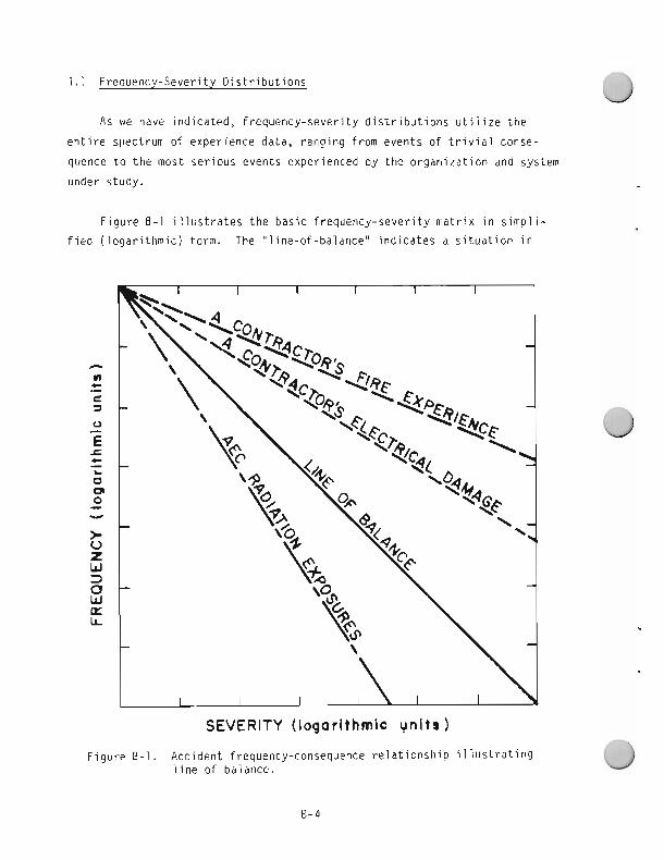
1.1 Frequency-Severity Distributions

As we have indicated, frequency-severity distributions utilize the

entire spectrum of experience data, ranging from events of trivial conse-

quence to the most serious events experienced by the organization and system

under study.

Figure 0-1 illustrates the basic frequency-severity matrix in simpli-

fied (logarithmic) form. The "line-of-balance" indicates a situation in

SEVERITY (logarithmic uni ts

Figure 0-1. Accident frequency-consequence relationship illustrating line of balance.

which losses a re balanced i n t h e sense t h a t a s i n g l e $1000 l o s s i s c o n t r o l -

l e d w i t h t h e same ef fec t iveness as one thousand $1.00 losses. Such balance

i s n o t n e c e s s a r i l y "good ' o r " b a d ' b u t forms a conven ient frame o f re fe rence

i n e v a l u a t i n g t h e n a t u r e of t h e c o n t r o l system.

As may be seen, t h e AEC r a d i a t i o n exposure d i s t r i b u t i o n i n d i c a t e s t h a t

t h e system i s r e l a t i v e l y pe rm iss i ve i n p e r m i t t i n g low l e v e l exposures, b u t

i s more r e s t r i c t i v e i n t h e upper exposure l e v e l s . Th i s r e s u l t i s n o t sur -

p r i s i n g if one s t u d i e s t h e n a t u r e o f t h e system c o n s t r a i n t s and c o n t r o l s

u t i l i z e d by AEC d u r i n g t h e p e r i o d under study.

The two c o n t r a c t o r d i s t r i b u t i o n s r e l a t i n g t o t h e f i r e and e l e c t r i c a l

l osses rep resen t a d i f f e r e n t s i t u a t i o n i n t h a t t h e system was more permis-

s i v e i n case o f t h e severe consequences. Th i s s i t u a t i o n has h i g h p o t e n t i a l

f o r r e s u l t i n g i n a " f o o l s parad ise" s i t u a t i o n . Th i s occurs because t h e h i g h

frequency events hav ing l e s s severe consequences a re o f t e n r e l a t i v e l y w e l l

c o n t r o l l e d . When t h e i n f r e q u e n t events having more se r i ous consequences

occur, t h e y may be t o o e a s i l y r a t i o n a l i z e d as unusual and i s o l a t e d events.

Th i s , i n f ac t , occur red t o some degree i n b o t h c o n t r a c t o r o rgan i za t i ons ,

whose performance i s i n d i c a t e d i n F i g u r e 0-1, and r e l a t i v e l y severe a c c i -

dents appeared as " s u r p r i s e s " due t o inadequate i n fo rma t i on and r e a c t i o n t o

t h e l e s s severe p recu rso r acc idents .

Once an acc iden t has occur red and t h e consequences a re evaluated, one

may d i r e c t l y e n t e r f requency-sever i ty d i s t r i b u t i o n s of t h e t ype i n d i c a t e d

i n F i g u r e 8-1 t o determine t h e expected frequency of such an acc iden t . An

a l t e r n a t i v e t o t h i s procedure i nvo l ves use of curves of t h e t ype shown i n

F i g u r e 8-2. The curves i n F i g u r e 8-2 a re ob ta ined by i n t e g r a t i n g t h e

f requency -seve r i t y curves t o o b t a i n t h e p r o b a b i l i t y o f exceeding a s p e c i f i e d

consequence l e v e l . F i g u r e 8-2 represents such a s tudy performed a number

of years ago r e l a t i n g t o r a d i o a c t i v e shipments.

The F i g u r e 8-2 curves i n d i c a t e t h e p r o b a b i l i t y of exceeding a g i ven

d o l l a r l o s s on a pe r shipment and on a pe r yea r bas i s f o r a g i ven o p e r a t i o n

( i d e n t i f i e d as t h e "ITS" ope ra t i on ) . Since t h e d e r i v a t i o n of p r e d i c t e d

l o s s f o r t h e o p e r a t i o n under s tudy was prepared l a r g e l y on t h e b a s i s of

t h e o r e t i c a l d a t a (due t o l a c k of a c t u a l acc ident da ta ) , AEC data, which

6-5

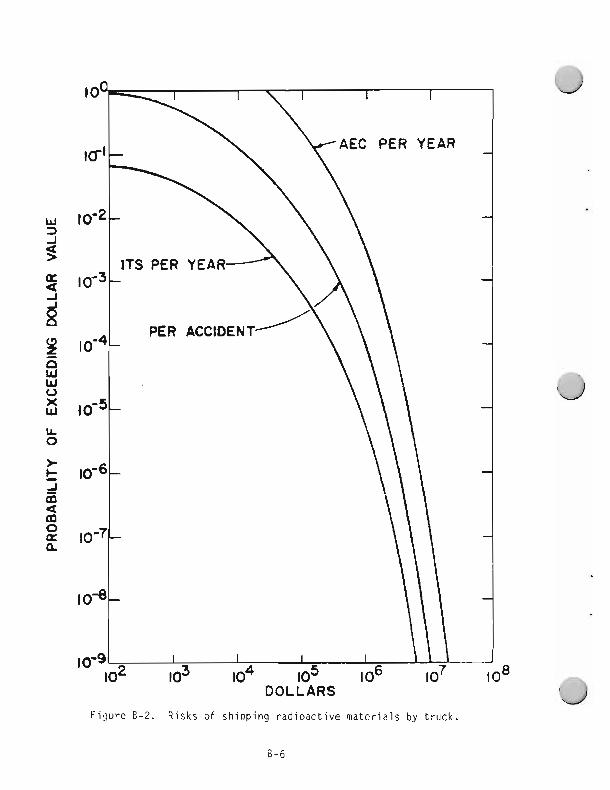
Figure 6-2. Risks of shipping radioactive materials by truck.

8 - 6

includes many more such shipments, were used to construct the "AEC" curve. This is done to provide an envelope and to evaluate the reasonableness of

predictions relating to the specific "ITS" operation.

1.2 Extreme Value Analysis

As indicated earlier, application of frequency-severity distributions

require use of all data generated by the organization ranging from low frequency-severe consequence to high frequency-low consequence levels.

Furthermore, these data may be distributed in a variety of ways which require sophisticated statistical analysis.

This leads to a number of difficulties in use of frequency-severity

distributions:

1. Large quantities of data must often be processed (the AEC radia- tion exposure curve in Figure 6-1 represents analysis of more than

one million pieces of data).

2. Low severity data are often not readily available or may not exist

at all (due to reporting thresholds).

3. The great mass of the data will ordinarily lie in the low severity

range. If one does not use extreme care in analysis, one can

arrive at a situation in which "the tail wags the dog" in the

sense that a large mass of low consequence data predominate in

predicting the severe consequence events (which we are interested

in).

4. One must use extreme care in selecting, using, and testing

statistical distribution functions in order to avoid invalid

conclusions.

This raises the question as to whether other predictive and analytical

0 methods exist which:

i. Require a smaller quantity of Inore readily available data

2. Are s e l f - t e r t i n g as t o a p p l i c a b i l i t y .

I The extreme va lue a n a l y s i s o f Gumbel represents such a method.

T h i s method i s descr ibed i n MORT and i n Gumbel's e x c e l l e n t monograph

referenced i n MORT. We w i l l no t go i n t o t h e d e t a i l e d t heo ry o r s p e c i f i c s

of a p p l i c a t i o n here. I n b r i e f , t h e method i nvo l ves :

1. S e l e c t i n g a p e r i o d o f homogeneous o p e r a t i o n p r i o r t o t h e even t

under study.

2. Break ing t h e p e r i o d o f t ime down i n t o app rop r i a te i n t e r v a l s .

3. Obta in ing t h e most severe consequence event f o r each o f t h e t i m e

i n t e r v a l s .

4. P l o t t i n g t h e worst-case events on t h e s p e c i a l extreme va lue paper

i n accordance w i t h t h e r u l e s p rov ided i n t h e MORT manual.

5. T e s t i n g f o r a p p l i c a b i l i t y . (Does t h e d a t a p l o t as a s t r a i g h t

l i n e ? )

6. Determin ing how t h e acc ident event r e l a t e s t o t h e normal system

behav ior as i n d i c a t e d by t h e remaining da ta p o i n t s .

7. S t r u c t u r i n g t h e i n v e s t i g a t i o n and recommendations i n accordance

w i t h I t em 6, above.

F igu res 8-3, -4, and -5 i n d i c a t e a p p l i c a t i o n o f extreme va lue a n a l y s i s

t o AEC p r o p e r t y l o s s data. F i g u r e 8-3 i n d i c a t e s t h e r e s u l t s us ing raw 1088

data . I n t h i s case, o n l y a smal l p o r t i o n o f t h e more r e c e n t d a t a f i t t h e

s t r a i g h t l i n e d i s t r i b u t i o n . Examinat ion of t h e da ta revea l s t h a t t h e

d o l l a r va lue o f AEC p r o p e r t y p laced a t r i s k , as w e l l as t h e p r o p e r t y

losses, grew a t a h i g h r a t e d u r i n g t h e p e r i o d under study, i .e. , t h e

s i t u a t i o n changed r a p i d l y .

T h i s suggests use of l o s s r a t i o s ( cen ts l o s s pe r $100 p r o p e r t y owned

by AEC). Loss r a t i o as a f u n c t i o n o f t ime i s i n d i c a t e d i n F i g u r e 8-4. If

one now p l o t s t h e l o s s r a t i o f i g u r e s on extreme va lue paper, it may be seen

0-8

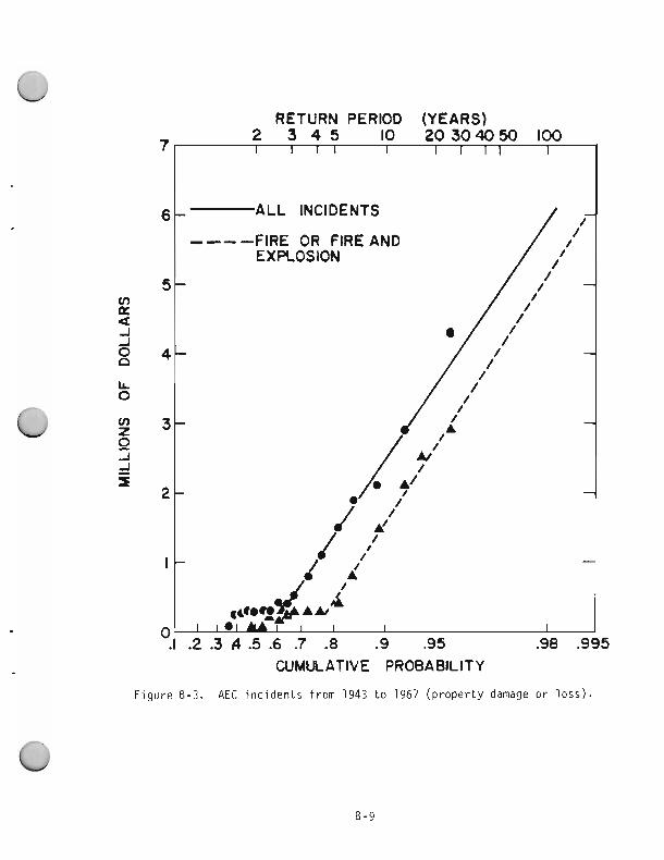
RETURN PERIOD (YEARS) 2 3 4 5 10 20 304050 100 I I I 1 I I I I I 1 1

Figure 8-3. AEC incidents from 1943 to 1967 ( p r o p e r t y damage o r loss).

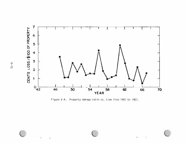
F i g u r e 8-4. P r o p e r t y damage r a t i o vs. t i m e f r o m 1947 t o 1967.

> 7 -

6.- a a 5 - LL 0 0 0 4 - Y, \

r n 3 - V) 0 ' 2 - V) C

1

I I I I 1 I I I I I I I I

-

0 -

0

w u '42 I 46 1 bAo.li/ I I I I I Y I e?\ I 1 0. / ! L I I ! 50 54 YEAR 58 62 66 70

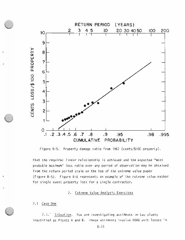
Figure 8-5. Property damage ratio from 1967 (cents/$lOO property).

RETURN PERIOD ( Y E A R S )

1 0 r 2 3 4 5 10 20 30 4050 100 2 0 0

that the required linear relationship is achieved and the expected "most

probable maximum" loss ratio over any period of observation may be obtained

from the return period scale on the top of the extreme value paper

(Figure B-5). Figure 8-6 represents an example of the extreme value method

for single event property loss for a single contractor.

9 -

8 -

2. Extreme Value Analysis Exercises

I I I I I I I I I I

-

-

2.1 Case One

7-

6 -

5 -

4-

- I

.I .2 .3.4.5 .6 .7 .8 .9 .95 .98 .995 CUMULATIVE PROBABILITY

2.1.1 Situation. You are investigating accidents in two plants

identified as Plants A and B. These accidents involve 6000 unit losses in

B-11

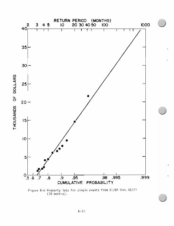
RETURN PERIOD (MONTHS) 2 3 4 5 10 2 0 3 0 4 0 5 0 100

40 DO0

I I I I I I I I I I

' 7 I

F i g u r e 8 - 6 P r o p e r t y l o s s f o r s i n g l e e v e n t s f r o m 01 /68 t h r u 02 /71 ( 3 8 months ) .

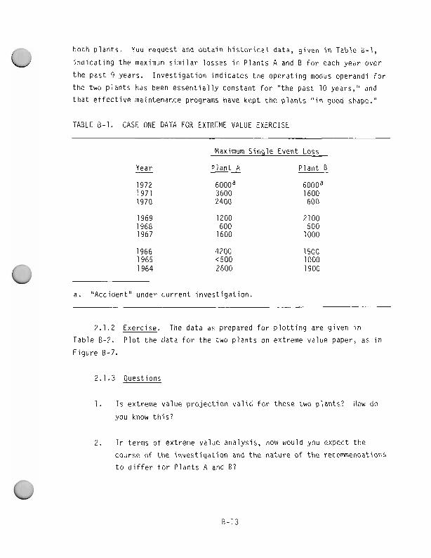
bo th p lants . You request and o h t a i n h i s t o r i c a l data, g i ven i n Table 0-1,

i n d i c a t i n g the maximun s i m i l a r losses i n P lan ts A and B f o r each year over

t h e past 9 years. I n v e s t i g a t i o n i n d i c a t e s the opera t ing modus operandi f o r

t he two p l a n t s has been e s s e n t i a l l y constant f o r " the past 10 years," and

t h a t e f f e c t i v e maintenance programs have kept t h e p l a n t s " i n good shape."

TABLE 0-1. CASE ONE DATA FOR EXTREME VALUE EXERCISE

Maximum S ing le Event Loss

Year - Plant A P lan t B

a. "Accident4' under c u r r e n t i nves t iga t i on .

2.1.2 Exercise. The data as prepared f o r p l o t t i n g are g iven i n

Table 8-2. P l o t t he da ta f o r the two p l a n t s on extreme value paper, as i n

F igu re 8-7.

2.1.3 Quest ions

1. I s extreme va lue p r o j e c t i o n v a l i d f o r these two p l a n t s ? How do

you know t h i s ?

2. I n terms o f extreme value analysis, how would you expect t h e

course o f t h e i n v e s t i g a t i o n and t h e nature o f t h e recommendations

t o d i f f e r f o r P lan ts A and B?

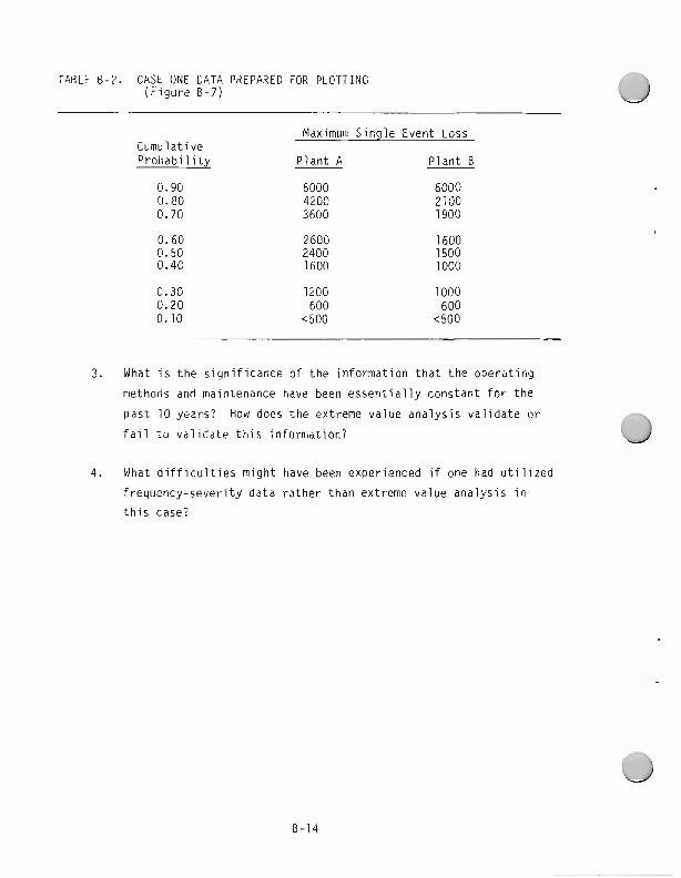
TABLE 8-2. CASE ONE DATA PREPARED FOR PLOTTING ( F i g u r e 8-7)

Maximum S i n g l e Event Loss Cumulat ive P r o b a b i l i t y P l a n t A P l a n t B

0.90 6000 6000 0.80 4200 2100 0.70 3600 1900

3. What i s t h e s i g n i f i c a n c e o f t h e i n fo rma t i on t h a t t h e o p e r a t i n g

methods and maintenance have been e s s e n t i a l l y constant f o r t h e

p a s t 10 yea rs? How does t h e extreme va lue a n a l y s i s v a l i d a t e o r

f a i l t o v a l i d a t e t h i s i n f o r m a t i o n ?

4. What d i f f i c u l t i e s m igh t have been exper ienced i f one had u t i l i z e d

f requency -seve r i t y d a t a r a t h e r t han extreme va lue a n a l y s i s i n

t h i s case?

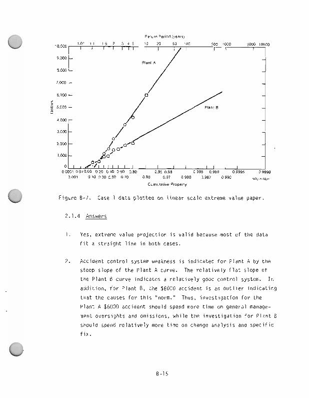
0 F i g u r e 8-7 . Case 1 d a t a p l o t t e d on l i n e a r s c a l e extreme va lue paper.

1. Yes, extreme va lue p r o j e c t i o n i s v a l i d because most of t h e d a t a

f i t a s t r a i g h t l i n e i n b o t h cases.

2. Acc ident c o n t r o l system weakness i s i n d i c a t e d f o r P l a n t A by t h e

steep s lope of t h e P l a n t A curve. The r e l a t i v e l y f l a t s l ope of

t h e P l a n t 0 cu rve i n d i c a t e s a r e l a t i v e l y good c o n t r o l system. I n

a d d i t i o n , f o r P l a n t 0, t h e $6000 acc iden t i s an o u t l i e r i n d i c a t i n g

t h a t t h e causes f o r t h i s "norm." Thus, i n v e s t i g a t i o n f o r t h e

P l a n t A $6000 acc iden t should spend more t i m e on genera l manage-

ment o v e r s i g h t s and omissions, w h i l e t h e i n v e s t i g a t i o n f o r P l a n t B

shou ld spend r e l a t i v e l y more t ime on change a n a l y s i s and Spec i f i c

f i x .

3. There have been no major changes which would change o r d i s t o r t

t h e acc iden t f r equency -seve r i t y d i s t r i b u t i o n . The f a c t t h a t t h e

da ta do f i t a s t r a i g h t l i n e v a l i d a t e s t h a t no e x t e r n a l i n f l u e n c e

has pe r tu rbed t h e system.

4. It i s u s u a l l y more d i f f i c u l t t o o b t a i n c o n s i s t e n t da ta on a l l

acc iden ts over a 10-year per iod , t h a t i s t o ge t i n f o r m a t i o n about

t h e l a r g e s t acc ident . I n a d d i t i o n , a much l a r g e r q u a n t i t y of

d a t a must be analyzed.

2.2 Case Two

2.2.1 S i t u a t i o n . You a re i n v e s t i g a t i n g f a t a l acc iden ts i n two

c o n t r a c t o r o r g a n i z a t i o n s i d e n t i f i e d as Con t rac to rs X and Y. N e i t h e r

o r g a n i z a t i o n had exper ienced a f a t a l i t y d u r i n g t h e p a s t 10 years. You

reques t and r e c e i v e d i s a b l i n g i n j u r y d a t a f o r t h e two p l a n t s i n terms of

t h e maximum d i s a b l i n g i n j u r y d u r i n g each 6-month p e r i o d f o r t h e p a s t

10 years. When t h e d a t a a re ranked accord ing t o magnitude and r e l a t e d t o

cumu la t i ve p r o b a b i l i t y i n t h e usua l manner, t h e r e s u l t s i n d i c a t e d i n

Table 8-3 a re obtained.

2.2.2 Exercise. P l o t t h e d a t a i n Table 8-3 on t h e l i n e a r sca le

extreme va lue paper, as i n F i g u r e 8-8, on t h e l o g s c a l e extreme va lue

paper, as i n F i g u r e B-9, f o r both con t rac to rs .

2.2.3 Ques t i ons

1. Which r e p r e s e n t a t i o n i s more app rop r i a te f o r Con t rac to r X , t h e

l i n e a r or t h e l o g sca le?

2. The s t a t i s t i c i a n advises us t h a t t h e l o g r e p r e s e n t a t i o n i s more

a p p r o p r i a t e f o r s i t u a t i o n s i n which t h e l i m i t s do n o t e x i s t on

how bad t h i n g s can ge t a t t h e h i g h s e v e r i t y end of t h e curve. I n

t h i s l i g h t , what can we say about bas i c energy-safe ty c o n t r o l s i n

t h e Con t rac to r X o r g a n i z a t i o n ?

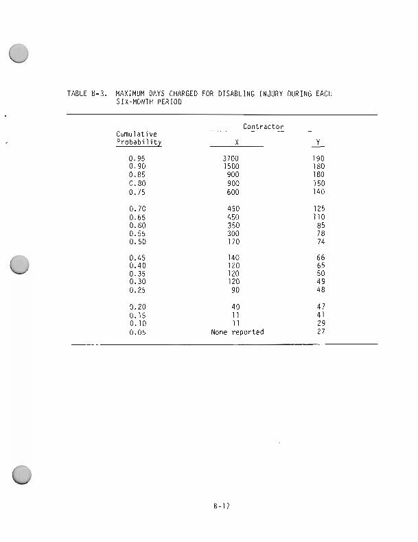
TABLE 8-3. MAXIMUM DAYS CHARGED FOR DISABLING INJURY DURING EACH SIX-MONTH PERIOD

Cumulative Probabilitz

0.95 0.90

Contractor

X Y

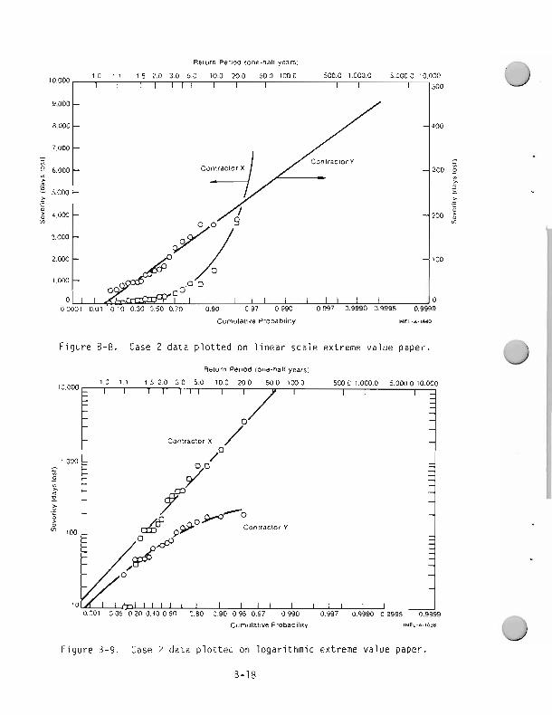
~ e t ~ r n P ~ O O (one naif years]

100oO i 0 i l 1 5 2 0 3 0 5 0 TOO 2 0 0 5 0 0 7000 5 0 0 0 1 0 0 0 0 5 0 0 0 0 10000

I 1 I I I 1 1 1 I I I I I 1 I 1500

Cumuiaflve Probablllty I N L L - A - ~ ~ ~ ~

Figure B-8. Case 2 data plotted on linear scale extreme value paper.

Return Perloa lone-halt years)

u 1 1 1 1 1 1 1 1 1 1 I 1 1 , l I / I , I J 0.001 0.05 0 20 0.40 0 60 0.80 0 90 0 95 0 9 7 0.990 0.997 0.9990 0 9995 0.9999

I Cumulative Probablllty ~ E 1 - ~ - 2 6 1 8

w Figure B-9. Case 2 data plotted on logarithmic extreme value paper.

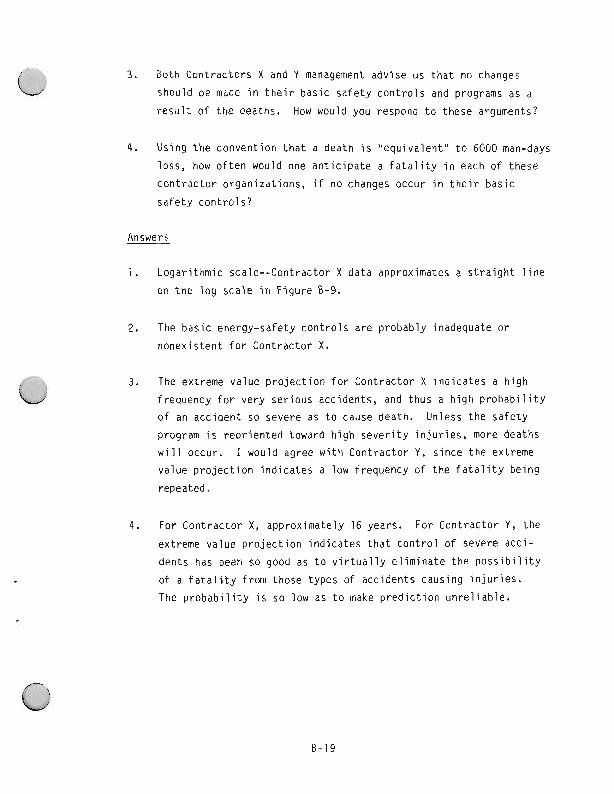
3. Both Contractors X and Y management advise us that no changes Should be made in their basic safety controls and programs as a

result of the deaths. How would you respond to these arguments?

4. Using the convention that a death is ''equivalent" to 6000 man-days

loss, how often would one anticipate a fatality in each of these

contractor organizations, if no changes occur in their basic

safety controls?

I. Logarithmic scale--Contractor X data approximates a straight line

on the log scale in Figure 0-9.

2. The basic energy-safety controls are probably inadequate or

nonexistent for Contractor X.

0 3. The extreme value projection for Contractor X indicates a high

frequency for very serious accidents, and thus a high probability

of an accident so severe as to cause death. Unless the safety

program is reoriented toward high severity injuries, more deaths

will occur. I would agree with Contractor Y, since the extreme value projection indicates a low frequency of the fatality being

repeated.

4. For Contractor X, approximately 16 years. For Contractor Y, the extreme value projection indicates that control of severe acci-

dents has been so good as to virtually eliminate the possibility

of a fatality from those types of accidents causing injuries.

The probability is so low as to make prediction unreliable.

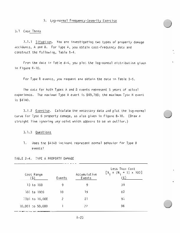
3. Log-normal Frequency-Severity Exercise

3.1 Case Three

3.1.1 Situation. You are investigating two types of property damage accidents, A and 6. For Type A, you obtain cost-frequency data and construct the following, Table 6-4.

From the data in Table 8-4, you plot the log-normal distribution given

in Figure 6-10.

For Type 6 events, you request and obtain the data in Table B-5

The data for both Types A and B events represent 5 years of actual experience. The maximum Type A event is $49,700; the maximum Type B event is $4140.

3.1.2 Exercise. Calculate the necessary data and plot the log-normal

curve for Type 6 property damage, as also given in Figure 6-10. (Oraw a straight line ignoring any point which appears to be an outlier.)

3.1.3 Questions

1 . Does the $4140 incident represent normal behavior for Type 6 events?

TABLE 6-4. TYPE A PROPERTY DAMAGE

Less Than Cost

Cost Range Accumu 1 at i ve [Ni + ( N . 1 + 1) x 1001

( $ 1 Events Events (%)

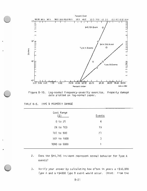
percent Under !NEL-C~~J I

F i g u r e 6-10. Log-normal f r equency -seve r i t y exe rc i se . P rope r t y damage d a t a p l o t t e d on log-normal paper.

TABLE 8-5. TYPE B PROPERTY DAMAGE

Cost Range ( 3 )

0 t o 25

26 t o 100

101 t o 500

501 t o 1000

1000 t o 5000

Events

6

19

21

3

1

2. Does t h e $49,700 i n c i d e n t rep resen t normal behav ior f o r Type A

events?

3. V e r i f y y o u r answer by c a l c u l a t i n g how o f t e n i n years a >650,000

Type A and a >$4000 Type B event would occur. ( H i n t : From t h e

Percent over scale, determine what fraction of the events exceed

the cost value in question. From this and the number of events

per year, the frequency in years can be calculated.)

4. With regard to the $4140 incident, should one be more concerned with the control system or specific condition requiring correc-

tion? With regard to the $49,700 incident?

5. From the data, which cost ranges represent the greatest risk for

Types A and 8 events? (risk = expected loss = consequence x

frequency - the relative risks may be approximated by the average cost in each range multiplied by the number of events in that

range.)

6. When should log-normal be used rather than extreme value?

1. No, the $4140 Type 6 event is an outlier.

2. Yes, the $49,700 Type A event lies close to the curve and is part

of the log-normal population.

3. The 22 Type A accidents in the 5-year period are equivalent to 100 accidents in 22.7 years. From Figure 6-10, the $50,000

severity level occurs at approximately 2.8 "percent over," which

indicates that for each 100 accidents, 2.8 accidents each greater

than $50,000 will occur each 22.7 years or one $50,000 accident

each 8 years. (Or, 2.8% of 4.4 accidentslyear is 0.123 accidents

greater than $50,00O/year: 110.123 = 8.) The 50 Type 6 accidents

in the 5-year period are equivalent to 100 accidents in 10 years.

From Figure 8-10, approximately 0.20 accidents greater than $4000 will occur for each 100 accidents in the 10-year interval or

1 accident greater than $4000 each 50 years. (Or, 0.2% of

50 accidentslyear is 2 x lo-' accidentslyear, or 50 years1

accident for those greater than $4000.)

4. For the $4140 incident, the specific condition requiring

correction should be sufficient. The control system applicable

to Type B events should be investigated in addition to correcting

the specific condition. (MORT analysis should be done in each

case; it is more urgent for the Type A events.)

5. For Type A events, the top severity range is most important (one $50,000 event is worse than two $10,000 events, etc.). For Type B events, the $100 to $500 range represents the greatest

loss.

6 . Log-normal should be used when the number of events in each time period is small, or when additional information beyond predicting

the return period for large events is desired.

4. Log-Loq Frequency-Severity Exercise

4.1 Case Four

4.1.1 Situation. You desire further analysis of the Types A and B

data given in the log-normal exercise. You transfer the Type A log-normal curve (accumulative frequency vs. severity) to log-log paper, using the

"percent over" and "cost greater than" values. (This curve is shown in

Figure 6-11.)

4.1.2 Exercise. Transfer the Type B log-normal curve (accumulative

frequency vs. severity) to log-log paper.

4.1.3 Questions

1. Compare the two log-log curves for Types A and B events. Which

curve has the greatest slope? (Note that the risk is increasing

where the slope is <1 and decreasing where the slope >I.)

0 2. What are the peculiar advantages of log-normal and log-log curve?

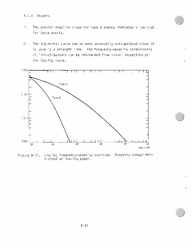
1 . The greater negative slope for Type B events indicates a low risk

for large events.

2. The log-normal curve can be more accurately extrapolated since it

is usually a straight line. The frequency-severity relationship or line-of-balance can be determined from visual inspection of

the log-log curve.

Figure 6-11. Log-log frequency-severity exercise. Property damage data plotted on log-log paper.

APPENDIX C

PROBABILITY AN0 STATISTICS PRIMER

This appendix provides a basic introduction to probability theory and

statistical distribution. Some additional detail is provided in the body of the report. Many textbooks and references are available for further study. Recommended are "Introduction to Statistical Analysis' by

W. J. Dixon and F. J. Massey and "Statistical Analysis" by Bennet and

Franklin (particularly Chapter I1 for trend analysis and tests for

randomness), TEAM Associates, P.O. Box 25 Tamworth, NH 03886, can provide

graph paper and methods for their use.

The theory of probability deals with the chance occurrence of random

events. Random, as defined in the dictionary, means lacking a specific

pattern or causal relationship, haphazard. Chance refers to the nature of unpredictable events. An example is that of nine black balls and one white ball in a black bag. What is the chance of picking a white ball? The

position of the balls and the selection are completely uncontrolled; thus

each ball has an equal chance of being picked. The probability is

simple--1 chance in 10 or 0.1. However, if the experiment is repeated

100 times, the white ball would not necessarily be picked 10 times. The best we can predict is that it would be picked 10 t X times, the value of X depending upon probability theory. It is possible that the white ball could be picked any number of times from 0 to 100 times. The likelihood of

any number in this range can be calculated. Of course, the chance of the

white ball being picked 100 times is virtually zero, it being (a decimal fraction preceded by 100 zeros).

Chance events are not determined by luck, but are events which result

from activities from which more than one outcome is possible. Chance also refers to an unplanned event which results from a combination or interaction of conditions and/or activities which are not sufficiently

monitored to permit a prediction of the exact time and place of occurrence. As such, accidents are chance events which can be analyzed using probability and statistics. A person who habitually crosses a road

without looking will eventually be hit by a vehicle, but without knowing

the exact time of crossing or passing of vehicles, we cannot predict which

crossing will result in the accident. With sufficient crossing and traffic information, we could, however, deduce the probability of being hit by a

vehicle.

Probability refers to the chance or likelihood of a specific event

occurring given an opportunity for its occurrence. Probability values range from zero (impossible to occur) to 1.0 (certain to occur). A probability of 0.5 means that the occurrence or nonoccurrence is equally likely. While probability refers to the likelihood of a specific event given a single

Opportunity for its occurrence, statistics deal with the number of times an

event will occur given many opportunities. Statistics also deal with the

variation in the "probable' numbers of events. For example, if we toss a

coin 10 times, the probable number of heads is 5. This means that if we

repeated the 10 tosses many times, 5 heads would occur most frequently.

The frequency of 4 or 6 heads would be less frequent, 3 or 7 heads even

less frequent, and so on. The relative frequency of the number of heads

falls into a well-defined pattern, called a statistical distribution of a

variable. The variable is the number of heads in the experimental

10 tosses.

These two concepts of (a) probability of an event and (b] the

statistical distribution of variables are fundamental to risk analyses. A

few basic laws of probability and a discussion of statistical distributions

are presented in this section.

1. Probability

Mathematically, probability is defined as the number of tilnes an event

will produce a given result divided by the total number of events. The

probability value can be deduced or inferred. For example, with a throw of

a single die, there are six possible outcomes or numbers. Any particular

number (say a 5) has 1 chance in 6. Thus, the probability of a 5 is 1/6.

This is a deduced probability and is exact if the die is not loaded and is

in perfect symmetry. 0

If we cannot determine t h e e q u a l i t y and number of outcomes th rough

reasoning, t h e n we can, by t r i a l , determine t h e approximate p r o b a b i l i t y .

If we throw t h e d i e 36 t imes, and t h e 5 comes up o n l y 5 i ns tead o f 6 t imes,

we would s t i l l conc lude (because of t h e smal l number of t r i a l s ) t h a t t h e

p r o b a b i l i t y of a 5 i s 1/6, n o t 5/36. On t h e o t h e r hand, i f we suspected t h a t t h e d i e was loaded, we m igh t conclude t h a t t h e p r o b a b i l i t y o f a 5 was

about 5/36, b u t c o u l d be 6/36 o r even 4/36. Our bes t es t ima te i s 5/36.

Now, if t h e d i e were thrown 36,000 t imes, and a 5 comes up 5,000 t imes, we

conclude t h a t t h e d i e i s indeed loaded, and t h e p r o b a b i l i t y o f a 5 i s v e r y

c l o s e t o 5,000/36,000 ( o r 5/36) and v e r y l i k e l y n o t 6/36 o r 4/36. Th i s

p r o b a b i l i t y of 5/36 i s i n f e r r e d from observat ion . S t a t i s t i c s i s t h e

mathematics of inference.

The domain of s t a t i s t i c a l in ference i nc ludes b o t h e s t i m a t i n g p r o b a b i l -

i t y and i t s u n c e r t a i n t y f r om p rev ious exper ience (how many t imes it has

occur red i n t h e pas t ) , and e s t i m a t i n g how many t imes something w i l l happen

based on a deduced p r o b a b i l i t y . The accuracy o f these es t ima tes i s a l s o

determined from s t a t i s t i c s . P r o b a b i l i t y can be r e l a t i v e l y exac t i f deduced

from known c o n d i t i o n s . A coin, d ie, r o u l e t t e wheel, a l l have ve ry exac t

p r o b a b i l i t i e s . Bu t even though t h e p r o b a b i l i t y of an outcome i s known v e r y

p r e c i s e l y , t h e r e s u l t s o f a smal l number of t r i a l s cannot be p r e c i s e l y

p red i c ted .

The most common method o f e s t i m a t i n g t h e p r o b a b i l i t y o f an acc iden t i s

from p rev ious exper ience. I f a c o n t r a c t o r has exper ienced 5 i n j u r i e s f o r

each 100 employees, t h e average employee i n j u r y p r o b a b i l i t y i s 0.05. T h i s

va lue m u l t i p l i e d by t h e number o f employees w i l l es t ima te t h e number o f

i n j u r i e s f o r t h e n e x t year. I n p r o b a b i l i t y language t h i s es t imated number

i s c a l l e d t h e "expected" number and i s r e f e r r e d t o as "expectat ion." An

average p r o b a b i l i t y va lue may be g r o s s l y m is lead ing if app l i ed t o an

i n d i v i d u a l , who may have a r e l a t i v e l y h i g h e r o r lower r i s k t han average.

There a re no ha rd g u i d e l i n e s f o r avo id ing e r r o r s when app l y i ng a

genera l average t o a s p e c i f i c s i t u a t i o n o r v i c e versa. However, t h e

p o p u l a t i o n from which a p r o b a b i l i t y i s es t imated shou ld be as s i m i l a r as

p r a c t i c a l t o t h e p o p u l a t i o n t o which i t i s app l ied . Even though smal l

groups within the population vary significantly, if the two populations

have the same small group distribution, the variations within the two

populations will average out.

For example, to estimate a vehicle accident probability:

1. Use U.S. Moter Vehicle Accident Statistics from the National

Safety Council's "Accident Facts" for the average probability of

a U.S. citizen

2 . Use DOE vehicle statistics for the average probability of a DOE

employee

3. Use the contractor experience for the average contractor employee

4. However, for a DOE bus driver, use national professional bus

driver statistics if DOE bus statistics are unavailable.

Conditional probability is the probability of a consequence conditioned

upon a prerequisite event. For example, what is the probability of an

injury if a vehicle accident occurs? This conditional probability is

obtained by dividing the number of injuries by the number of accidents. To

obtain the probability of an injury per mile of travel, multiply the

accident probability by the conditional probability:

in'uries Probability of injurylmile = accidentslmile x ac:idents

The probability of an injurylmile can be obtained directly by dividing the

number of injuries by the number of miles, but the example illustrates the

concept of conditional probability.

Using this concept one can objectively estimate the probability of a

fatality even though no fatalities have occurred, using the ratio of

injuries to fatalities based on experience. Extreme care should be used in

applying one type of experience to another because these ratios (or

conditional probabilities) may vary widely.

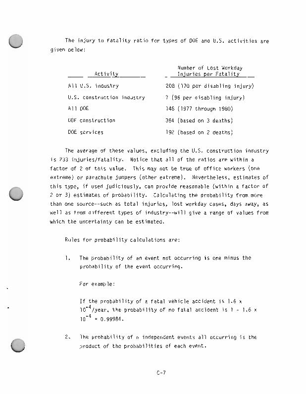
The injury to fatality ratio for types of DOE and U.S. activities are

given below:

Number of Lost Workday Activity Injuries per Fatality

All U.S. industry 208 (170 per disabling injury)

U.S. construction industry ? (96 per disabling injury)

All DOE 148 (1977 through 1980)

DOE construction 384 (based on 3 deaths)

DOE services 192 (based on 2 deaths)

The average of these values, excluding the U.S. construction industry

is 233 injurieslfatality. Notice that all of the ratios are within a

factor of 2 of this value. This may not be true of office workers (one

extreme) or parachute jumpers (other extreme). Nevertheless, estimates of

this type, if used judiciously, can provide reasonable (within a factor of

2 or 3) estimates of probability. Calculating the probability from more

than one source--such as total injuries, lost workday cases, days away, as well as from different types of industry--will give a range of values from

which the uncertainty can be estimated.

Rules for probability calculations are:

1. The probability of an event not occurring is one minus the probability of the event occurring.

For examole:

If the probability of a fatal vehicle accident is 1.6 x 4 10- /year, the probability of no fatal accident is 1 - 1.6 x

= 0.99984.

0 2. The probability of n independent events all occurring is the

product of the probabilities of each event.

For example:

The probability of two individuals both dying in a vehicle 4 2 accident in any 1 year is (1.6 x 10 or 2.56 x 10'~. The

probability of both living is 0.99984 x 0.99984 or 0.99968.

Further, the probability of one individual not being killed in

n years is 0.99984~.

3. The probability of at least one event occurring is one minus the

probability of no event. (The probabilities for all possible

outcomes always total one.)

For example:

The probability of at least one of the two individuals having a

fatal accident is one minus no fatal accident or 1 - 0.99968 or 3.2 x

4. Small probabilities (<0.10) may be added with little error to

determine the probability of either (any one) event occurring.

For example:

Small probabilities may be added (<0.1) with little error. The probability of either of two individuals having an accident is

4 1.6 x + 1.6 x or 3.2 x 10- .

2. Statistics

Common statistical terms and definitions are:

Distribution The frequency or manner in which observations of

different values are distributed over the range of

values. These values can be numbers, frequency, size,

cost, severity, etc.

Frequency

distribution

Mode

Mean

Median

Variance

Standard

deviation

Skewed

The relative frequency with which a variable quantity

or variate assumes particular values.

The most common or frequent observation or value.

The arithmetic average of all observations or values.

The point at which half the observations or values lie

above and half below.

A measure of dispersion or variation in observations values. It is the summation of the squared difference

between the mean and each value in the distribution,

divided by the number of observations or values.

The square root of the variance. It is a standard

measure of dispersion: in the normal distribution for

example, it is 68, 95, and 99.7% of all values occur

between tl, 2, or 3 standard deviations from the mean, respectively. Statistical tables provide values

from which we can determine the fraction of observations lying within a specified deviation.

The distribution is skewed if it is not balanced or

symetric around the mean. Most distributions found

in nature, including accidents, are skewed. The

reason is simple. In a symmetric distribution the mean is half way between the smallest and largest

possible values. In nature, the largest value is usually more than twice the average, and frequently many times the average. Another example: with an

average of only three accidents per year, zero is the

fewest possible while more than six is possible. The

smaller the average value relative to the maximum

Possible value, the greater the degree of skewness.

Conf idence

Range

Cumulat ive

f requency

( p r o b a b i l i t y )

Extreme va lue

Re tu rn p e r i o d

Dens i t y

f u n c t i o n

H is togram

Most probab le

maximum va lue

The chance of l i k e l i h o o d t h a t a s p e c i f i e d va lue i s

p a r t of t h e p o p u l a t i o n ( i f a s p e c i f i c va lue l i e s

o u t s i d e i t h r e e standard d e v i a t i o n s f rom t h e mean,

t hen we have 99.7% conf idence t h a t t h i s obse rva t i on i s

d i f f e r e n t than t h e p o p u l a t i o n s i nce 99.7% o f t h e

p o p u l a t i o n l i e s i n t h a t range).

A measurement o f t h e d i f f e rence between two

observat ions . The e n t i r e range i s t h e d i f f e r e n c e

between t h e sma l l es t and l a r g e s t value. We a l s o speak

of t h e i n n e r two q u a r t i l e range which i nc ludes 50% o f

a l l va lues (exc lud ing t h e sma l l es t 25% and t h e l a r g e s t

25%).

The frequency o r p r o b a b i l i t y which i nc ludes (o r

accumulates) a l l obse rva t i ons above o r below a

sDec i f ied va lue.

The l a r g e s t obse rva t i on d u r i n g a g i ven p e r i o d of

obse rva t i on .

The average space o r t i m e i n t e r v a l between a g i v e n

obse rva t i on . (A $10,000 acc iden t w i l l occur eve ry

10 years.) Th i s va lue i s t h e r e c i p r o c a l o r i n v e r s e o f

t h e frequency, and i s equal t o 111 - p, where p i s t h e

cumu la t i ve p r o b a b i l i t y .

The va lue o f t h e y - a x i s on a p r o b a b i l i t y d i s t r i b u t i o n

cu rve (see F i g u r e C-2 l a t e r i n t h i s Appendix). I t i s

a measure of f requency o f s t a t e d va lues on t h e x -ax is .

P i c t o r i a l r e p r e s e n t a t i o n of a d i s t r i b u t i o n ; a bargraph.

The r e t u r n p e r i o d measures how o f t e n an event equal t o

o r g r e a t e r t han a s p e c i f i e d va lue w i l l occur. T h i s

s p e c i f i e d va lue i s t h e probab le maximum value.

P r o b a b i l i t y A s p e c i a l graph paper i n which t h e x -ax i s and y - a x i s

paper a re sca led i n such a way as t o conve r t a d i s t r i b u t i o n

cu rve i n t o a s t r a i g h t l i n e . The purpose i s t w o f o l d - - a

s t r a i g h t l i n e f u n c t i o n i s ( a ) e a s i e r t o f i t and

( b ) e a s i e r t o e x t r a p o l a t e . The t e s t t o determine t h e

t ype o f d i s t r i b u t i o n i s : what t ype of p r o b a b i l i t y

paper r e s u l t s i n a s t r a i g h t l i n e f i t . If t h e r e i s a

good s t r a i g h t l i n e f i t of t h e data, we can be reason-

a b l y su re t h a t t h e exper ience can be represented by

t h a t t y p e o f d i s t r i b u t i o n .

Acc iden ts occur as a r e s u l t of unplanned combinat ions of events and,

as such, a re s t a t i s t i c a l i n nature. By s t a t i s t i c a l , we mean t h e exact c o s t

o r t ime of a s p e c i f i c acc iden t cannot be p red i c ted . A smal l sample o f

acc iden ts appear t o be random w i t h no s p e c i f i c p a t t e r n o f f requency o r c o s t .

However, as t h e sample s i z e increases (exper ience i s accumulated), a p a t t e r n

beg ins t o emerge i n t h a t we can beg in t o es t ima te t h e average number of

acc iden ts which w i l l occur i n a g i ven t i m e p e r i o d and t h e r e l a t i v e f requency

w i t h which acc iden ts occur w i t h i n a g i v e n c o s t range (assuming t h e r e a re no

s i g n i f i c a n t changes i n t h e ma jo r f a c t o r s which cause these acc iden ts ) .

Th i s p a t t e r n i s c a l l e d a s t a t i s t i c a l d i s t r i b u t i o n and can be def ined

u s i n g a h is togram o r a p r o b a b i l i t y curve. F i g u r e C-1 d e p i c t s a h is togram

and p r o b a b i l i t y curve, g i v i n g t h e f r a c t i o n of yea rs ( p r o b a b i l i t y ) i n which

0, 1 2,. . . 10 acc iden ts would occur g i v e n an average of 5 acc iden ts1

year. The smooth l i n e approx imat ing t h e h is togram i s a p r o b a b i l i t y curve.

The shapes of va r i ous p r o b a b i l i t y curves a re determined by t h e funda-

mental processes such as count ing , a d d i t i o n , m u l t i p l i c a t i o n , exponen t i a t i on ,

o r combinat ions of these processes. Each process c rea tes a s t a t i s t i c a l d i s t r i b u t i o n , t h e p r o b a b i l i t y cu rve hav ing a unique i d e n t i f i a b l e shape

p e c u l i a r t o t h e process from which it o r i g i n a t e s .

These curves a re conver ted t o s t r a i g h t l i n e s by use of p r o b a b i l i t y

Paper w i t h s p e c i a l scales. A s p e c i a l t ype of p r o b a b i l i t y paper i s r e q u i r e d

f o r each t ype o f d i s t r i b u t i o n . P l o t t i n g t h e d a t a on va r i ous t ypes of

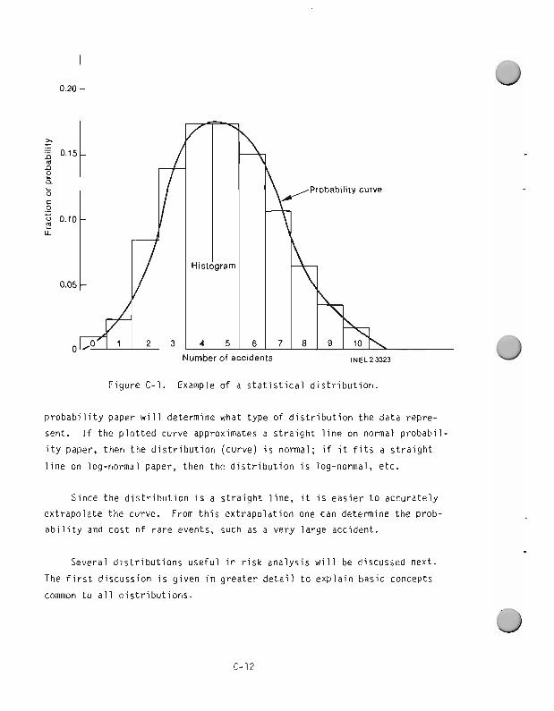
umber of accidents INEL 2 3323

Figure C-1. Example of a statistical distribution.

probability paper will determine what type of distribution the data repre-

sent. If the plotted curve approximates a straight line on normal probabil-

ity paper, then the distribution (curve) is normal; if it fits a straight

line on log-normal paper, then the distribution is log-normal, etc.

Since the distribution is a straight line, it is easier to accurately

extrapolate the curve. From this extrapolation one can determine the prob-

ability and cost of rare events, such as a very large accident.

Several distributions useful in risk analysis will be discussed next. The first discussion is given in greater detail to explain basic concepts

common to all distributions.

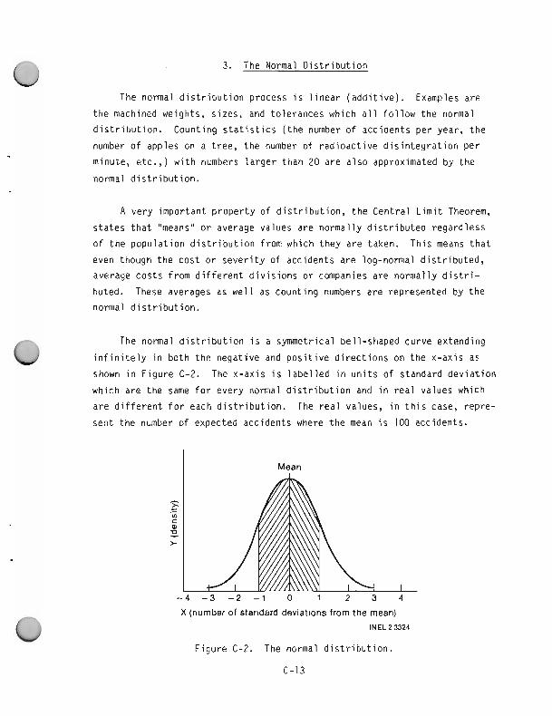
3. The Normal D i s t r i b u t i o n

The normal d i s t r i b u t i o n process i s l i n e a r ( a d d i t i v e ) . Examples a re

t h e machined weights, s izes , and to le rances which a l l f o l l o w t h e normal

d i s t r i b u t i o n . Count ing s t a t i s t i c s ( t h e number o f acc iden ts p e r year , t h e

number of apples on a t r ee , t h e number of r a d i o a c t i v e d i s i n t e g r a t i o n p e r

minute, etc.,) w i t h numbers l a r g e r t han 20 a re a l s o approximated by t h e

normal d i s t r i b u t i o n .

A v e r y impor tan t p r o p e r t y of d i s t r i b u t i o n , t h e Cen t ra l L i m i t Theorem,

s t a t e s t h a t "means" o r average va lues a re no rma l l y d i s t r i b u t e d rega rd less

of t h e p o p u l a t i o n d i s t r i b u t i o n from which t h e y a r e taken. Th i s means t h a t

even though t h e c o s t o r s e v e r i t y of acc iden ts a re log-normal d i s t r i b u t e d ,

average cos ts from d i f f e r e n t d i v i s i o n s o r companies a re no rma l l y d i s t r i -

buted. These averages as w e l l as coun t i ng numbers a re represented by t h e

normal d i s t r i b u t i o n .

The normal d i s t r i b u t i o n i s a symmetr ical be l l -shaped cu rve ex tend ing

i n f i n i t e l y i n b o t h t h e nega t i ve and p o s i t i v e d i r e c t i o n s on t h e x -ax i s as

shown i n F i g u r e C-2. The x - a x i s i s l a b e l l e d i n u n i t s of s tandard d e v i a t i o n

which a re t h e same f o r eve ry normal d i s t r i b u t i o n and i n r e a l va lues which

a r e d i f f e r e n t f o r each d i s t r i b u t i o n . The r e a l values, i n t h i s case, rep re -

sent t h e number of expected acc idents where t h e mean i s 100 acc idents .

X (number of standard deviations from the mean)

INEL23324

F i g u r e C-2. The normal d i s t r i b u t i o n .

C-13

Not a l l be l l -shaped symmetr ical curves a re normal d i s t r i b u t i o n curves.

The words "normal d i s t r i b u t i o n " r e f e r t o t h e f a c t t h a t t h e area under t h e 0 ' cu rve i s d i s t r i b u t e d i n a s p e c i f i e d manner which w i l l be d iscussed l a t e r .

T h i s area represents t h e r e l a t i v e frequency w i t h which v a r i a b l e s f a l l w i t h i n

two p o i n t s on t h e x -ax is . The p o i n t s on t h e x -ax i s a r e l a b e l l e d i n u n i t s

of standard d e v i a t i o n beg inn ing w i t h zero a t t h e c e n t e r w i t h nega t i ve va lues

ex tend ing t o t h e l e f t and p o s i t i v e va lues t o t h e r i g h t . These u n i t s of

standard d e v i a t i o n a re a l s o c a l l e d " Z scores." The h e i g h t of t h e cu rve i s

measured by p o i n t s along t h e y - a x i s which measures t h e " p r o b a b i l i t y den-

s i t y . " That i s , t h e h i g h e r t h e curve, t h e g r e a t e r t h e area and, hence, t h e

g r e a t e r t h e p r o b a b i l i t y between two p o i n t s on t h e x -ax is . For example,

between zero and one s tandard dev ia t i on , t h e p r o b a b i l i t y i s 0.34; between

one s tandard d e v i a t i o n and two s tandard dev ia t i ons , t h e p r o b a b i l i t y i s

0.135. The t o t a l area under t h e cu rve i s one square u n i t o r a p r o b a b i l i t y

of one. Thus t h e p r o b a b i l i t y ( a rea ) of 0.34 between 0 and 1 s tandard

d e v i a t i o n means t h a t 34% o f t h e v a r i a b l e s i n a normal d i s t r i b u t i o n f a l l

between 0 and 1 s tandard d e v i a t i o n . These p r o b a b i l i t y va lues ( i n terms of

s tandard d e v i a t i o n s ) a re g i v e n i n Table C-1. The mean i s denoted by u

and t h e s tandard d e v i a t i o n by o . By us ing s tandard d e v i a t i o n s and a

convers ion t a b l e i ns tead of l a b e l i n g t h e x - a x i s d i r e c t l y i n p r o b a b i l i t y

u n i t s , one se t o f va lues (one t a b l e ) i s a p p l i c a b l e t o d i s t r i b u t i o n o f any

average and any standard d e v i a t i o n .

The standard d e v i a t i o n i s c a l c u l a t e d from a se t of obse rva t i ons us ing

t h e f o l l o w i n g equat ion :

Standard D e v i a t i o n =\iF ( o r , square r o o t o f t h e va r i ance )

where

- X = t h e average va lue o f t h e v a r i a b l e a l s o denoted as u

Xi = t h e va lue each obse rva t i on o r v a r i a b l e

n = t h e number o f obse rva t i ons o r v a r i a b l e s .

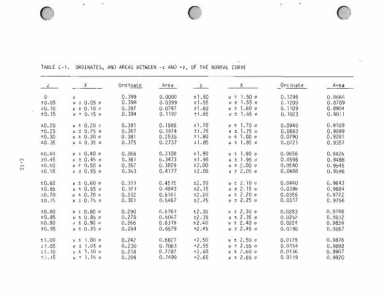
TABLE C-1. ORDINATES, AND AREAS BETWEEN - z AN0 + I , OF THE NORMAL CURVE

iO.60 50.65 i 0 . 7 0 i o . 75

t0.80 t0.85 i0 .90 to. 95

Ord ina te

0.399 0.398 0.397 0.394

0.391 0.387 0.381 0.375

0.368 0.361 0.352 0.343

0.333 0.323 0.312 0.301

0.290 0.278 0.266 0.254

0.242 0.230 0.218 0.206

Area

0.0000 0.0399 0.0797 0.1192

0.1585 0.1974 0.2538 0.2737

0.3108 0.3473 0.3829 0.4177

0.4515 0.4843 0.5161 0.5467

0.5763 0.6047 0.6319 0.6579

0.6827 0.7063 0.7287 0.7499

Ord ina te Area

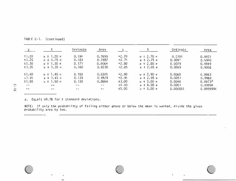
TABLE C-1. (continued)

z X Ordinate - Area z X Ordinate Area

f1.20 u i 1.20 o 0.194 0.7699 +2.70 u 2 2.70 o 0.0104 0.9931 i1.25 u i 1.25 o 0.183 0.7887 +2.75 u i 2.75 o 0.0091 0.9940 i1.30 u i 1.30 o 0.171 0.8064 +2.80 u 2 2.80 o 0.0079 0.9949 21.35 u i 1.35 o 0.160 0.8230 +2.85 u f 2.85 o 0.0069 0.9956

i1.40 u 2 1.40 o 0.150 0.8385 +2.90 u i 2.90 o 0.0060 0.9963 21.45 u f 1.45 o 0.139 0.8529 +2.95 u i 2.95 o 0.0051 0.9968 21.50 u i 1.50 o 0.130 0.8664 i3.00 u i 3.00 o -- 0.0044 -- -- -- 0.9973a

o t4.00 u i 4.00 a 0.0001 0.99994 J -- -- -- rn

-- f5.00 u f 5.00 o 0.000001 0.9999994

a. Equals 99.7% for * standard deviations. NOTE: If only the probability of falling either above or below the mean is wanted, divide the given probability area by two.

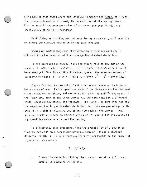
F o r coun t i ng s t a t i s t i c s where t h e v a r i a b l e i s mere ly t h e number o f events,

t h e standard d e v i a t i o n i s s imp ly t h e square r o o t o f t h e average number.

F o r i ns tance if t h e average number of acc iden ts p e r y e a r i s 100, t h e

s tandard d e v i a t i o n i s 10 acc idents .

M u l t i p l y i n g o r d i v i d i n g each obse rva t i on by a constant , w i l l m u l t i p l y

O r d i v i d e t h e standard d e v i a t i o n by t h e same constant .

Adding o r s u b t r a c t i n g each obse rva t i on by a cons tan t w i l l add o r

s u b t r a c t from t h e mean b u t w i l l n o t change t h e s tandard d e v i a t i o n .

To add s tandard dev ia t i ons , t a k e t h e square r o o t o f t h e sum o f t h e

squares of each s tandard d e v i a t i o n . F o r instance, i f Con t rac to r A and B

have averaged 100 + 10 and 49 t 7 acc idents lyear , t h e expected number of 2 acc iden ts f o r b o t h i s : 49 t 7 + 100 + 10 = 149 t 7 + 10' = 149 + 12.2.

F i g u r e C-3 d e p i c t s two s e t s of d i f f e r e n t normal curves. Each cu rve

has an area of one. I n t h e upper s e t each o f t h e t h r e e curves has t h e same

shape, s tandard dev ia t i on , and var iance; b u t each has a d i f f e r e n t mean. I n

t h e lower set, each of t h e t h r e e curves has t h e same mean b u t a d i f f e r e n t

shape, s tandard dev ia t i on , and var iance. The cu rve w i t h more area o u t near

t h e edges has t h e l a r g e r s tandard dev ia t i on , b u t t h e same percentage o f t h e

area f a l l s w i t h i n +1 s tandard dev ia t i on , f o r each o f t h e curves. Thus,

o n l y one t a b l e i s needed t o conve r t any va lue f o r any o f t h e s i x curves t o

a p r o b a b i l i t y va lue o r a p e r c e n t i l e rank ing.

To i l l u s t r a t e , t h i s procedure, f i n d t h e p r o b a b i l i t y of a d e v i a t i o n

f rom t h e mean > I 5 i n a p o p u l a t i o n hav ing a mean o f 100 and a s tandard

d e v i a t i o n o f 10. (Th i s i s a coun t i ng s t a t i s t i c a p p l i c a b l e t o t h e number of

i n j u r i e s o r acc idents . )

4. S o l u t i o n

1. D i v i d e t h e d e v i a t i o n (15) by t h e standard d e v i a t i o n (10) which

eaua ls 1.5 standard dev ia t i ons .

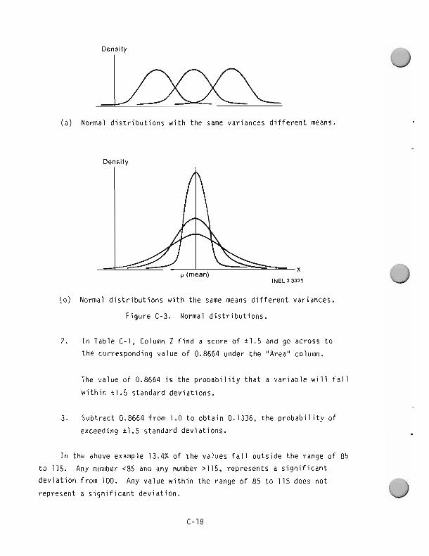
Density

( a ) Normal d i s t r i b u t i o n s w i t h t h e same var iances d i f f e r e n t means.

( b ) Normal d i s t r i b u t i o n s w i t h t h e same means d i f f e r e n t var iances.

F i g u r e C-3. Normal d i s t r i b u t i o n s .

2. I n Table C-1, Column Z f i n d a score o f +1.5 and go across t o

t h e cor respond ing va lue of 0.8664 under t h e "Area" column.

The va lue of 0.8664 i s t h e p r o b a b i l i t y t h a t a v a r i a b l e w i l l f a l l

w i t h i n i 1 .5 s tandard d e v i a t i o n s .

3. Sub t rac t 0.8664 f rom 1.0 t o o b t a i n 0.1336, t h e p r o b a b i l i t y o f

exceeding t1.5 s tandard d e v i a t i o n s .

I n t h e above example 13.4% o f t h e va lues f a l l o u t s i d e t h e range of 85

t o 115. Any number <85 and any number > l l 5 , r ep resen ts a s i g n i f i c a n t

d e v i a t i o n from 100. Any va lue w i t h i n t h e range o f 85 t o 115 does n o t

rep resen t a s i g n i f i c a n t d e v i a t i o n .

The degree of sureness or certainty is called the significance level.

It is an arbitrarily selected value used to test an assumption or a

hypothesis. This significance level is sometimes called a confidence

level. The confidence level or confidence interval refers to the mean when

it is not known but estimated from sampling or statistical measurement.

For example, in the above sample problem, if the mean is estimated from a

sample population of 1000 (10 measurements of 100 each) the mean is known to an accuracy of 100 2 3.2 standard deviations calculated as follows:

In either case, the procedure described above is used to determine the per-

cent of values with any range of values. The significance level is the

level or percent of time a single observation will fall within a population

range. The confidence level is the level or percent of a large number of

samples giving a mean or average within the stated range.

The procedure i n statistical testing is as follows:

1. State a hypothesis (make an assumption).

Example: A value of 85 represents a significant change from an average of 100.

2. Select a significance level.

Example: We want to be 90% sure we do not reject a good

statistic.

3. Test the hypothesis by determining the probability that the

variable is part of the population.

Example: A deviation of 15 (100 - 85) will occur 86.6% of the time as determined from Table C-1.

4. Re jec t t h e hypothes is s i nce 86.6% i s <go%. We conclude t h a t a

va lue of 85 does n o t rep resen t a s i g n i f i c a n t change. [However,

if t h e va lue had been 80, w i t h a l l e l s e t h e same, we would have 0

accepted t h e hypothes is , s i nce a d e v i a t i o n of 20 (100 - 80) w i l l

occur 95.45% of t h e t ime and t h i s i s more than 90%. Here we would

have concluded t h a t a va lue of 80 does rep resen t a s i g n i f i c a n t

change.]

I n t h e above examples, t h e t e s t i n g has been aga ins t exceeding a d e v i a t i o n

i n terms of abso lu te va lue ( g r e a t e r t han a p o s i t i v e o r nega t i ve d e v i a t i o n

of 15). Th i s t e s t i n g i s s a i d t o be two-sided s ince t h e p r o b a b i l i t y i nc ludes

t h e area on bo th s i des of t h e cu rve around t h e mean. One-sided t e s t i n g

r e f e r s t o t e s t i n g f o r o n l y a decrease ( o r an increase) . There a r e no one-

s ided p r o b a b i l i t y t a b l e s s i nce these va lues a r e j u s t one-ha l f o f t h e

two-s ided value.

F o r example, t h e p r o b a b i l i t y of <85 acc iden ts i s one-half t h e

0.13 va lue o r 0.065. The complementary va lue i s 0.935 and corresponds t o a

conf idence l e v e l t h a t 85 acc iden ts o r l e s s represents a s i g n i f i c a n t

reduc t i on . 0

T h i s may appear c o n t r a d i c t o r y t o t h e p rev ious conc lus ion t h a t a dev ia-

t i o n of 15 i s n o t s i g n i f i c a n t , b u t it i s n o t because s i g n i f i c a n c e i s d e t e r -

mined by an a r b i t r a r y p rese lec ted conf idence l e v e l . One can c o r r e c t l y

choose e i t h e r a two- o r one-sided conf idence l e v e l a t whatever degree of

conf idence i s des i red, depending on whether t h e t e s t i n g i s be ing done f o r

improvement o r mere ly change (good o r bad) as l ong as t h e choosing i s done

w i t h an unders tand ing of one- and two-s ided va lues and conf idence l e v e l s .

5. The Cumulat ive Normal D i s t r i b u t i o n

T h i s d i s t r i b u t i o n i s mere ly a d i f f e r e n t r e p r e s e n t a t i o n of t h e same

s t a t i s t i c a l p a t t e r n desc r i bed by t h e normal d i s t r i b u t i o n . Rather t han

g i v i n g t h e r e l a t i v e f requency w i t h which v a r i a b l e s f a l l on e i t h e r s i d e o f

t h e mean as i n t h e normal d i s t r i b u t i o n , t h e cumu la t i ve d i s t r i b u t i o n g i v e s

t h e r e l a t i v e f requency w i t h which obse rva t i ons w i l l f a l l below ( t o t h e l e f t

o f ) any s p e c i f i e d value. I n t h e upper (normal) d i s t r i b u t i o n cu rve i n 0

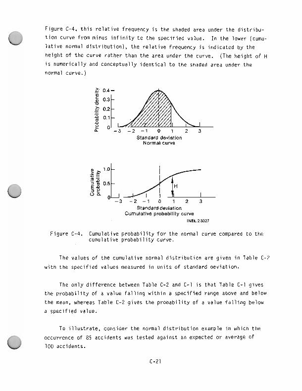
F igure C-4, t h i s r e l a t i v e frequency i s the shaded area under the d i s t r i b u -

0 t i o n curve from minus i n f i n i t y t o the spec i f ied value. I n t h e lower (cumu-

l a t i v e normal d i s t r i b u t i o n ) , the r e l a t i v e frequency i s i nd ica ted by the

he igh t of t h e curve r a t h e r than t h e area under the curve. (The he igh t o f H

i s numer ica l ly and conceptual ly i d e n t i c a l t o the shaded area under the

normal curve.)

2 0.4 m 5 0.3 D

5 0.2 - - 0.1

n e 0 P -3 -2 - 1 0 1 2 3

Standard deviation Normal curve

Standard deviation Cumulative probability curve

INEL 2 3327

F igure C-4. Cumulative p r o b a b i l i t y f o r t h e normal curve compared t o t h e cumulat ive p r o b a b i l i t y curve.

The values o f t h e cumulat ive normal d i s t r i b u t i o n are g iven i n Table C-2

w i t h t h e spec i f ied values measured i n u n i t s o f standard dev ia t ion.

The on ly d i f f e r e n c e between Table C-2 and C-1 i s t h a t Table C-1 g ives

the p r o b a b i l i t y of a value f a l l i n g w i t h i n a s p e c i f i e d range above and below

t h e mean, whereas Table C-2 g ives t h e p r o b a b i l i t y o f a value f a l l i n g below

a s p e c i f i e d value.

To i l l u s t r a t e , cons ider the normal d i s t r i b u t i o n example i n which t h e

0 occurrence o f 85 accidents was tes ted against an expected o r average of

100 accidents.

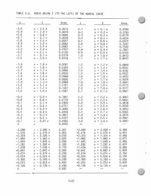
TABLE C-2. AREAS BELOW Z (TO THE LEFT) OF THE NORMAL CURVE

Area

0.0013 0.0019 0.0026 0.0035 0.0047 0.0062 0.0082 0.0107 0.0139 0.0179 0.0228

0.0287 0.0359 0.0446 0.0548 0.0668 0.0808 0.0968 0.1151 0.1357 0.1587

0.1841 0.2119 0.2420 0.2741 0.3085 0.3446 0.3821 0.4207 0.4602 0.5000

0.001 0.005 0.010 0.025 0.050 0.100 0.150 0.200 0.250 0.300 0.350 0.400 0.450 0.500

Area

0.5398 0.5793 0.6179 0.6554 0.6915 0.7257 0.7580 0.7881 0.8159 0.8413 0.8643

0.8849 0.9032 0.9192 0.9332 0.9452 0.9554 0.9641 0.9713 0.9772 0.9821

0.9861 0.9893 0.9918 0.0038 0.9953 0.9965 0.9974 0.9981 0.9987 --

0.999 0.995 0.990 0.975 0.950 0.900 0.850 0.800 0.750 0.700 0.650 0.600 0.550 --

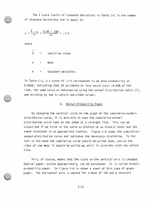
The Z score ( u n i t s of standard dev ia t ion ) i n Table C-2 i s the number

of standard dev ia t ions and i s equal t o :

where

- X = s p e c i f i e d v a l u e

II = mean

o = standard dev ia t ion.

I n Table C-2, a z score o f -1.5 corresponds t o an area p r o b a b i l i t y of

0.0668, i n d i c a t i n g t h a t 85 accidents o r l ess would occur <6.68% of t h e

time, the same value as obtained by us ing the normal d i s t r i b u t i o n t a b l e ( I ) ,

and d i v i d i n g by two t o ob ta in one-sided values.

6. Normal-Probabi l i ty Paper

By changing t h e v e r t i c a l sca le on the graph o f the cumulative-normal-

d i s t r i b u t i o n curve, i t i s poss ib le t o have the cumulative-normal-

d i s t r i b u t i o n curve take on the shape o f a s t r a i g h t l i n e . Th is can be

v i s u a l i z e d if we t h i n k of the curve as p l o t t e d on an e l a s t i c sheet and t h e

sheet s t re tched i n an appropr ia te fashion. F igure C-5 shows the cumulat ive-

no rma l -d i s t r i bu t ion curve and ind ica tes the necessary s t re tch ing . To the

l e f t o f the mean the cumulat ive curve should be p u l l e d down, and on the

r i g h t of t h e mean i t should be p u l l e d up u n t i l i t co inc ides w i t h t h e do t ted

l i n e .

This, of course, means t h a t the sca le on the v e r t i c a l ax i s i s changed.

Special paper, scaled appropr ia te ly , can be purchased. I t i s c a l l e d normal-

p r o b a b i l i t y paper. I n F igure C-6 i s shown a sheet of t h i s type of graph

paper. The hor i zon ta l ax i s i s marked f o r a mean o f 100 and a standard

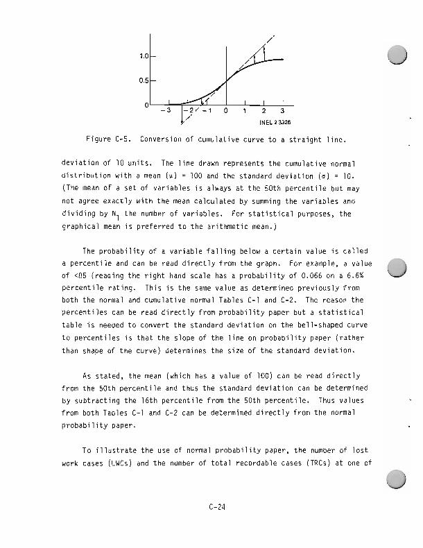
O - 3 -2,-, i

INEL23326

Figure C-5. Conversion of cumulative curve to a straight line.

deviation of 10 units. The line drawn represents the cumulative normal

distribution with a mean (u) = 100 and the standard deviation (0) = 10.

(The mean of a set of variables is always at the 50th percentile but may

not agree exactly with the mean calculated by summing the variables and

dividing by N1 the number of variables. For statistical purposes, the

graphical mean is preferred to the arithmetic mean.)

The probability of a variable falling below a certain value is called

a percentile and can be read directly from the graph. For example, a value of <85 (reading the right hand scale has a probability of 0.066 on a 6.6%

percentile rating. This is the same value as determined previously from

both the normal and cumulative normal Tables C-1 and C-2. The reason the

percentiles can be read directly from probability paper but a statistical

table is needed to convert the standard deviation on the bell-shaped curve

to percentiles is that the slope of the line on probability paper (rather

than shape of the curve) determines the size of the standard deviation.

As stated, the mean (which has a value of 100) can be read directly

from the 50th percentile and thus the standard deviation can be determined

by subtracting the 16th percentile from the 50th percentile. Thus values

from both Tables C-1 and C-2 can be determined directly from the normal

probability paper.

To illustrate the use of normal probability paper, the number of lost

work cases (LWCs) and the number of total recordable cases (TRCs) at one of

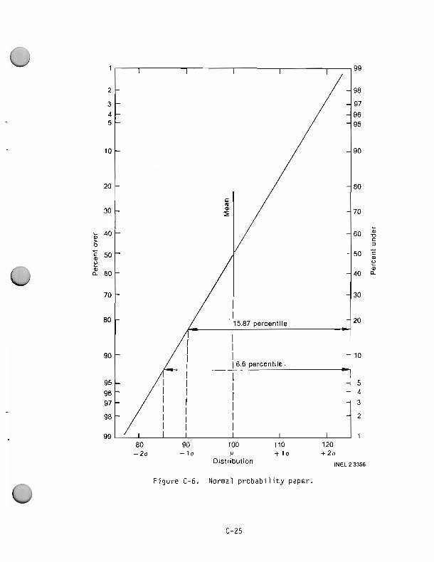
Figure C-6. Normal probability paper

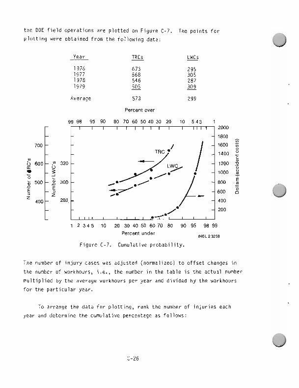
t h e DOE f i e l d ope ra t i ons a re p l o t t e d on F igu re C-7. The p o i n t s f o r p l o t t i n g were obta ined from t h e f o l l o w i n g data :

Year TRCs - LWCS -

Average 573 299

Percent ovet

1 2 3 4 5 10 20 30 40 50 60 70 80 90 95 98 99

Percent under INEL23358

F i g u r e C-7. Cumulat ive p r o b a b i l i t y .

The number of i n j u r y cases was ad jus ted (normal ized) t o o f f s e t changes i n

t h e number o f workhours, i.e., t h e number i n t h e t a b l e i s t h e a c t u a l number

m u l t i p l i e d by t h e average workhours pe r yea r and d i v i d e d by t h e workhours

f o r t h e p a r t i c u l a r year.

To ar range t h e d a t a f o r p l o t t i n g , rank t h e number o f i n j u r i e s each

yea r and determine t h e cumu la t i ve percentage as f o l l o w s :

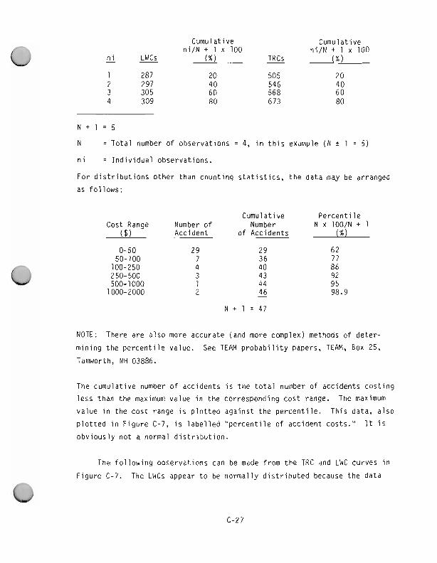
Cumulat ive Cumulat ive n i / N + 1 x 100 n i / N + 1 x 100

n i - - LWCs ( % I - TRCs ( % I

N + 1 = 5

N = T o t a l number o f obse rva t i ons = 4, i n t h i s example (N + 1 = 5 )

n i = I n d i v i d u a l observat ions .

F o r d i s t r i b u t i o n s o t h e r t han coun t i ng s t a t i s t i c s , t h e d a t a may be arranged

as f o l l o w s :

Cumulat ive P e r c e n t i l e Cost Range Number o f Number N x 100/N + 1

(6) Acc ident of Acc idents ( % )

NOTE: There a r e a l s o more accura te (and more complex) methods o f d e t e r -

m in ing t h e p e r c e n t i l e va lue. See TEAM p r o b a b i l i t y papers, TEAM, Box 25,

Tamworth, NH 03886.

The cumu la t i ve number of acc iden ts i s t h e t o t a l number of acc iden ts c o s t i n g

l e s s t han t h e maximum va lue i n t h e cor respond ing c o s t range. The maximum

va lue i n t h e c o s t range i s p l o t t e d aga ins t t h e p e r c e n t i l e . Th i s data, a l s o

p l o t t e d i n F i g u r e C-7, i s l a b e l l e d " p e r c e n t i l e o f acc ident costs." It i s

o b v i o u s l y n o t a normal d i s t r i b u t i o n .

The f o l l o w i n g obse rva t i ons can be made f rom t h e TRC and LWC curves i n

F i g u r e C-7. The LWCs appear t o be no rma l l y d i s t r i b u t e d because t h e d a t a

f i t a s t r a i g h t l i n e . The standard d e v i a t i o n i s about 15 cases (ob ta ined b y

read ing t h e number o f cases a t t h e 16 th p e r c e n t i l e o r a t t h e 84 th p e r c e n t i l e

and t a k i n g t h e d i f f e rence f rom t h e 50th p e r c e n t i l e ) . The coun t i ng s tandard

d e v i a t i o n i s t h e square r o o t of t h e annual number (299), which equa ls 17.

The good agreement i n d i c a t e s t h e degree o f v a r i a b i l i t y i s normal so t h a t

t h e r e i s no t r e n d as c y c l i c a l in f luences changing t h e LWC acc iden t

f requency.

On t h e o t h e r hand, t h e TKC d a t a do n o t f i t a s t r a i g h t l i n e . The

50th p e r c e n t i l e va lue i s 550 as opposed t o t h e a r i t h m e t i c average of

573 cases. The s tandard d e v i a t i o n f rom t h e cu rve between t h e 1 6 t h and

50th p e r c e n t i l e s i s about 60 compared t o t h e "square r o o t " s tandard dev ia -

t i o n of 24. We conc lude t h e TRC da ta a re n o t no rma l l y d i s t r i b u t e d , i n d i -

c a t i n g an i n c r e a s i n g o r decreas ing t rend. The l a r g e r standard d e v i a t i o n

i n d i c a t e s a l a r g e v a r i a t i o n , which i s always t h e case if a t r e n d e x i s t s .

C y c l i c a l v a r i a t i o n s w i t h no t r e n d w i l l a l s o produce a l a r g e s tandard dev ia-

t i o n , b u t w i l l f i t a s t r a i g h t l i n e . A bar graph r e p r e s e n t a t i o n o f these

d a t a i s g i ven i n F igu res C-8 and C-9. (The da ta on t h e normal p r o b a b i l i t y

paper correspond t o t h e LWC and TRC inc idence r a t e ba r graphs f o r o n l y t h e

years 1976 through 1979.) The LWC r a t e s f o r these yea rs a re cons tan t w i t h i n

one decimal p lace. The second decimal p lace i s i n s i g n i f i c a n t compared t o

normal s t a t i s t i c a l v a r i a t i o n and i s t h e r e f o r e n o t used. By con t ras t , t h e

TRC ba r graphs show a s i g n i f i c a n t downward t rend . Thus, normal p r o b a b i l i t y

paper i s a s p e c i a l g raph i c rep resen ta t i on w i t h p e r c e n t i l e s ( cumu la t i ve

percentages i n d i c a t e d r i g h t on t h e graph).

The v e h i c l e acc iden t c o s t d a t a a l s o do n o t f i t a s t r a i g h t l i n e and

demonstrate g r a p h i c a l l y t h a t acc ident c o s t d a t a do no t f i t t h e normal d i s -

t r i b u t i o n . Log-normal o r extreme va lue paper shou ld be used f o r p l o t t i n g

acc iden t c o s t versus f requency as d iscussed l a t e r i n t h i s appendix.

Whi le a cu rve on p r o b a b i l i t y paper i n d i c a t e s a t rend, two r u l e s O f

thumb can be used t o determine a t r e n d on t h e ba r graphs: ( a ) The o v e r a l l

d e v i a t i o n i s l a r g e compared t o d e v i a t i o n s between ad jacent years. For

example, i n F i g u r e C-9 t h e l a r g e d i f f e r e n c e between 1976 and 1980 i n d i c a t e s

a t rend. The increase i n 1981 over 1980 i s t o o smal l t o i n d i c a t e a r e v e r s a l

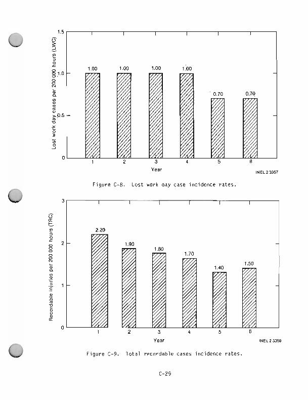
Year INEL 2 3357

F i g u r e C-8. Lost work day case i n c i d e n c e r a t e s .

Year 1 ~ ~ ~ 2 3 3 5 9

F i g u r e C-9. T o t a l r e c o r d a b l e cases inc idence r a t e s .

in the trend; (b) A persistent change in one direction for three or more

consecutive years indicates a trend. [The probability of a decrease is 0.5

(as much chance of decreasing as increasing) so that three such changes is 3

(0.5) or 0.125, indicating an 87.5% confidence level that there is a decreasing trend.]

These concepts also apply to curve fitting. Is a curve (or straight line) clearly identified by the data points, or is the scatter too great?

A subjective feel for goodness of fit is usually adequate for tentative

conclusions and/or identification of direction for further safety investi-

gation. Those who desire confidence limit tests for goodness of fit should

consult a textbook or a statistician.

As stated earlier, the normal distribution has limited application to

risk analyses. This extended discussion provides an understanding of dis- tributions and probability papers which are applicable to the log-normal

and extreme value distributions.

7. Log-Normal Distribution

Processes in which the effects are multiplied fit the log-normal

distribution. If the scale which measures the variable is logarithmic

rather than linear, the curve representing this distribution has the

symmetrical bell-shape of the normal curve. (An equivalent explanation is

the logarithm of the variable is substituted for the variable to produce

the same bell-shaped curve.)

On a linear scale, the log-normal curve is skewed with the peak to the

left of center and a long tail to the right. Examples of this distribution

are corrosion, gaseous diffusion, personal income, growth, and accident

severity.

An example of log-normal probability paper is given in Figure C-10.

it is identical to normal probability with the exception that the scale

measuring the variable is logarithmic rather than linear. On both papers,

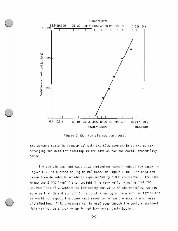
Percent over

0.5 1 5 10 20 30 40 50 6070 80 90 95 99 99.5 99.9

Percent under INEL23360

F i g u r e C-10. Veh i c l e acc iden t cos t .

t h e pe rcen t sca le i s symmetr ical w i t h t h e 50 th p e r c e n t i l e a t t h e cen te r .

A r rang ing t h e d a t a f o r p l o t t i n g i s t h e same as f o r t h e normal p r o b a b i l i t y

paper.

The v e h i c l e acc iden t c o s t d a t a p l o t t e d on normal p r o b a b i l i t y paper i n

F i g u r e C-7, i s p l o t t e d on log-normal paper i n F i g u r e C-10. The d a t a a re

t aken f rom 46 v e h i c l e acc iden ts exper ienced by a DOE c o n t r a c t o r . The da ta

below t h e $1000 l e v e l f i t a s t r a i g h t l i n e v e r y w e l l . Knowing t h a t t h e

maximum l o s s o f a v e h i c l e i s l i m i t e d by t h e va lue of t h e veh i c l es , we can

surmise t h a t t h i s d i s t r i b u t i o n i s cons t ra ined by an i nhe ren t l i m i t a t i o n and

we would n o t expect t h e upper c o s t range t o f o l l o w t h e l o g a r i t h m i c normal

d i s t r i b u t i o n . T h i s procedure can be used even though t h e v e h i c l e acc iden t

d a t a may n o t be a t r u e o r u n l i m i t e d log-normal d i s t r i b u t i o n .

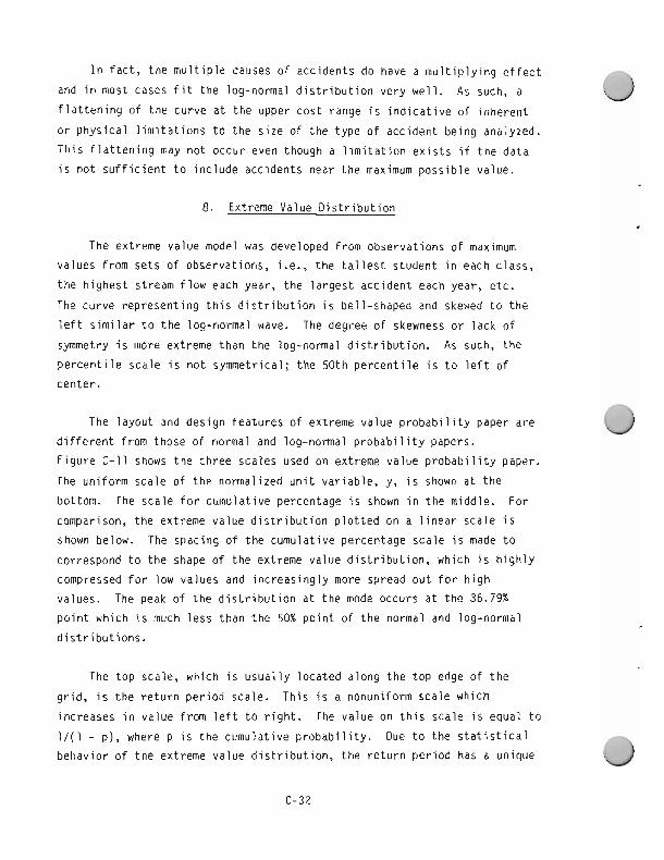
I n fac t , t h e m u l t i p l e causes of acc iden ts do have a m u l t i p l y i n g e f f e c t

and i n most cases f i t t h e log-normal d i s t r i b u t i o n ve ry w e l l . As such, a

f l a t t e n i n g of t h e curve a t t h e upper c o s t range i s i n d i c a t i v e of i n h e r e n t

o r p h y s i c a l l i m i t a t i o n s t o t h e s i z e of t h e t ype of acc iden t be ing analyzed.

T h i s f l a t t e n i n g may n o t occur even though a l i m i t a t i o n e x i s t s i f t h e d a t a

i s n o t s u f f i c i e n t t o i n c l u d e acc iden ts near t h e maximum p o s s i b l e value.

8. Extreme Value D i s t r i b u t i o n

The extreme va lue model was developed from obse rva t i ons of maximum

va lues f rom s e t s of observat ions , i.e., t h e t a l l e s t s tuden t i n each c lass ,

t h e h i g h e s t stream f l o w each year, t h e l a r g e s t acc iden t each year, e t c .

The cu rve rep resen t i ng t h i s d i s t r i b u t i o n i s be l l -shaped and skewed t o t h e

l e f t s i m i l a r t o t h e log-normal wave. The degree of skewness o r l a c k o f

symmetry i s more extreme than t h e log-normal d i s t r i b u t i o n . As such, t h e

p e r c e n t i l e sca le i s n o t symmetr ical ; t h e 50 th p e r c e n t i l e i s t o l e f t of

center .

The l ayou t and des ign fea tu res o f extreme va lue p r o b a b i l i t y paper a re

d i f f e r e n t from those o f normal and log-normal p r o b a b i l i t y papers.

F i g u r e C-11 shows t h e t h r e e sca les used on extreme va lue p r o b a b i l i t y paper.

The un i fo rm sca le o f t h e normal ized u n i t va r i ab le , y, i s shown a t t h e

bottom. The sca le f o r cumu la t i ve percentage i s shown i n t h e middle. For

comparison, t h e extreme va lue d i s t r i b u t i o n p l o t t e d on a l i n e a r sca le i s

shown below. The spac ing of t h e cumula t ive percentage sca le i s made t o

correspond t o t h e shape o f t h e extreme va lue d i s t r i b u t i o n , which i s h i g h l y

compressed f o r low va lues and i n c r e a s i n g l y more spread o u t f o r h i g h

values. The peak o f t h e d i s t r i b u t i o n a t t h e mode occurs a t t h e 36.79%

p o i n t which i s much l e s s t han t h e 50% p o i n t o f t h e normal and log-normal

d i s t r i b u t i o n s .

The t o p scale, which i s u s u a l l y l oca ted a long t h e t o p edge o f t h e

g r i d , i s t h e r e t u r n p e r i o d scale. Th i s i s a nonuni form sca le which

increases i n va lue from l e f t t o r i g h t . The va lue on t h i s sca le i s equal t o

1 / ( 1 - p ) , where p i s t h e cumula t ive p r o b a b i l i t y . Due t o t h e s t a t i s t i c a l

behav ior o f t h e extreme va lue d i s t r i b u t i o n , t h e r e t u r n p e r i o d has a un ique

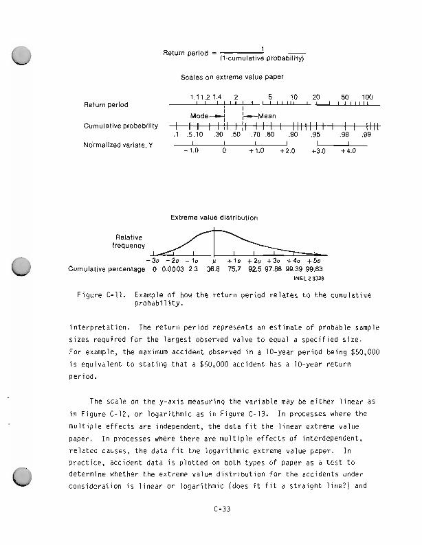
1 Return period =

(1-cumulative probability)

Scales on extreme value Paper

1.1 1.2 1.4 2 5 10 20 50 100 Return period I i I ~ I I t t 1 1 1 1 1 1 1 I I I 1 1 1 1 1 1 1

i I Mode* *Mean

Cumulative probability I

. .;.:o ' do" .do1' .;ol.do ' .dd ' I '.d5' ' 8 . 9 P

Normalized variate, Y I I I I I I - 1.0 0 +l.O +2.0 +3.0 +4.0

Extreme value distribution

Relative frequency

Cumulative percentage 0 0.0003 2.3 36.8 75.7 92.5 97.86 99.39 99.83

F igure C-11. Example o f how t h e r e t u r n p e r i o d r e l a t e s t o t h e cumulat ive p r o b a b i l i t y .

i n t e r p r e t a t i o n . The r e t u r n pe r iod represents an est imate o f probable sample

s izes requ i red f o r the la rges t observed valve t o equal a spec i f ied size.

For example, the maximum accident observed i n a 10-year pe r iod being $50,000

i s equiva lent t o s t a t i n g t h a t a $50,000 accident has a 10-year r e t u r n

per iod.

The sca le on the y -ax is measuring the va r iab le may be e i t h e r l i n e a r as

i n F igure C-12, o r l ogar i thmic as i n F igure C-13. I n processes where the

m u l t i p l e e f f e c t s are independent, the data f i t the l i n e a r extreme value

paper. I n processes where the re are m u l t i p l e e f f e c t s o f interdependent,

r e l a t e d causes, the data f i t t h e logar i thmic extreme value paper. I n

p rac t i ce , accident data i s p l o t t e d on both types of paper as a t e s t t o

determine whether the extreme value d i s t r i b u t i o n f o r the accidents under

cons iderat ion i s l i n e a r o r l ogar i thmic (does i t f i t a s t r a i g h t l i n e ? ) and

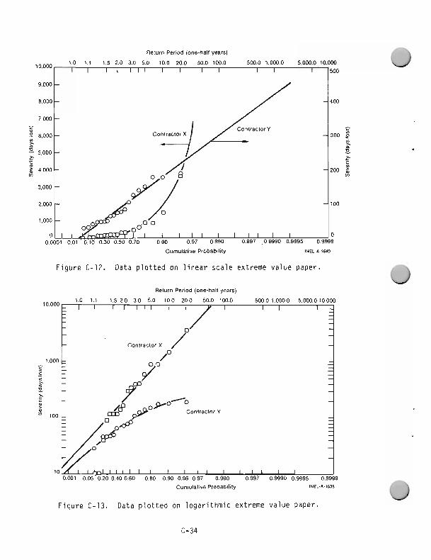
~ e t u r n period (one-half years)

,o,o 1 0 1.1 1.5 2.0 3.0 5.0 100 20.0 50.0 fW.0 5W.O l.OW.O 5.OW.010,OW

9,000

8.000

7 , m - - -0 6,000 ,.

5.000 .. 5 a p 4,OW m

3.000

2,WO

,,OW

0 0.0

Cumulative Probability #NEL~A-,M

Figure C-12. Data plotted on linear scale extreme value paper.

Return Period (one-half years)

contractor X /"

Cumulative Probability M S L - A - ? ~ ~

Figure C-13. Data plotted on logarithmic extreme value paper.

hence whether t h e m u l t i p l e acc ident causes are independent o r r e l a t e d by

some system weakness i n t h e c o n t r o l program. For example, t h e acc ident

curves f o r Cont ractor X and Y are bo th p l o t t e d on l i n e a r and loga r i t hm ic

extreme value paper i n F igures C-12 and C-13. As can be seen, t h e s e v e r i t y

f o r Cont ractor X increases more r a p i d l y than does t h e s e v e r i t y and t h e

curve f o r Cont ractor Y i n d i c a t i n g a much h igher p o t e n t i a l f o r a very severe

accident. I n add i t i on , t h e f a c t t h a t Cont ractor Y's data f i t a s t r a i g h t

l i n e on l i n e a r paper i n d i c a t e s t h a t t h e m u l t i p l e causat ion of acc idents are

r e l a t i v e l y independent. On t h e o the r hand, t h e interdependency i n d i c a t e d

by t h e s t r a i g h t l i n e f i t of Cont ractor X's data suggest common c o n t r i b u t i n g

f a c t o r s t o acc ident causat ion which cou ld be co r rec ted by s t rengthening t h e

safe ty program r a t h e r than look ing f o r a s p e c i f i c f i x .

9. Binomial D i s t r i b u t i o n

The b inomia l d i s t r i b u t i o n occurs i n problems i n which we take samples

from a l a r g e popu la t i on w i t h spec i f i ed "success" o r " f a i l u r e " p r o b a b i l i t i e s

and want t o eva luate t h e chances of ob ta in ing a c e r t a i n number of successes

i n the sample. As such, i t i s a count ing s t a t i s t i c . It has many appl ica-

t i o n s i n q u a l i t y con t ro l , r e l i a b i l i t y , consumer sampling, and many o t h e r

f i e l d s .

The v a r i a t i o n o r a d i s t r i b u t i o n o f t h e number o f occurrences

(acc idents) such as i s c a l c u l a t e d from t h i s fundamental law of

p r o b a b i l i t y . The b inomia l equat ion i s :

where

B = t h e p r o b a b i l i t y o f e x a c t l y r success i n n t r i a l s

r = number o f successes (occurrences)

n = n of t r i a l s ( t o t a l poss ib le number)

p = p r o b a b i l i t y of success (occur rence)

q = p r o b a b i l i t y of n o t o c c u r r i n g ( 1 - P)

! = f a c t o r i a l , which i s ( n x n - 1 x n - 2 x . . . 1).

F o r l a r g e va lues of n, i t approximates t h e normal d i s t r i b u t i o n (wh ich

i s e a s i e r t o use). For smal l va lues o f n, t h e Po isson d i s t r i b u t i o n i s

e a s i e r t o use. The b inomia l equat ion, however, i s r i g o r o u s l y d e r i v e d from

p r o b a b i l i t y combinat ion t h e o r y us ing a d i f f e r e n t i a l equat ion se r i es , and

thus i s n o t an approx imat ion b u t a c c u r a t e l y c a l c u l a t e s t h e exac t p r o b a b i l i t y

of r success i n n t r i a l s . I t shou ld be used when accuracy i s impor tan t o r

when redundancy i s used t o reduce r i s k i n those s i t u a t i o n s where one o r two

f a i l u r e s can be t o l e r a t e d , b u t a l a r g e r number o f f a i l u r e s would have

s e r i o u s consequences.

10. Poisson D i s t r i b u t i o n

The Poisson d i s t r i b u t i o n i s a l s o a coun t i ng s t a t i s t i c and approximates

t h e b inomia l d i s t r i b u t i o n when t h e average number o f events i s f i v e o r l ess .

It i s an approximate model f o r t h e number o f e lements p e r u n i t t i m e o r

space.

The Poisson d i s t r i b u t i o n has many a p p l i c a t i o n s i n q u a l i t y c o n t r o l ,

r e l i a b i l i t y , queuing theory , medica l and b i o l o g i c a l s t a t i s t i c s , and many

o t h e r f i e l d s . I n p a r t i c u l a r , t h i s d i s t r i b u t i o n may be an a p p r o p r i a t e model

f o r t h e number of de fec ts i n a p i e c e o f m a t e r i a l , t h e number of insurance

c la ims i n a g i v e n pe r i od , t h e number o f incoming c a l l s p e r m inu te on a

swi tchboard d u r i n g a p a r t i c u l a r t ime o f day, t h e number o f b a c t e r i a i n a

g i v e n c u l t u r e , t h e number of a lpha p a r t i c l e s em i t t ed f rom a r a d i o a c t i v e

source i n a s p e c i f i e d t ime i n t e r v a l , t h e number o f customer a r r i v a l s i n a

s t o r e a t a g i ven t i m e of day, and t h e number o f acc iden ts i n a s h o r t t i m e

per iod . The Poisson equa t i on i s :

where

P =

n =

X =

t h e p r o b a b i l i t y of e x a c t l y x events g i ven an average o f n

events

average number of events

t h e number of events f o r which t h e p r o b a b i l i t y i s be ing

ca l cu la ted .

The Poisson equa t i on r e q u i r e s o n l y a knowledge of t h e average number

of events t o determine t h e p r o b a b i l i t y of a s p e c i f i e d number o f events.

( I f t h e average number o f acc iden ts p e r y e a r i s f i v e , what i s t h e

p r o b a b i l i t y of e i g h t acc iden ts l yea r? ) Thus i t s use i s n o t l i m i t e d (as i s

t h e b inomia l equa t i on ) t o s i t u a t i o n s where t h e p r o b a b i l i t y o f success o r

f a i l u r e and t h e number of t r i a l s known. Note t h a t t h e average number ( n )

i s equal t o t h e number o f t r i a l s m u l t i p l i e d by t h e p r o b a b i l i t y (Np) and

t h i s p roduc t can be s u b s t i t u t e d f o r n i n t h e Poisson equat ion .

I n a d d i t i o n , as i n a l l coun t i ng s t a t i s t i c s as exp la ined i n t h e

d i scuss ion of t h e normal d i s t r i b u t i o n , t h e square r o o t o f t h e average

number o f events i s eaual t o t h e s tandard dev ia t i on .

The Poisson equa t i on i s recommended t o determine whether a d e v i a t i o n

from a smal l number o f events i s s t a t i s t i c a l l y s i g n i f i c a n t .

F o r example, i s an i n d i v i d u a l w i t h seve ra l acc iden ts a h i g h r i s k ? I s

t h e number o f acc iden ts i n a g i v e n department o r t ime p e r i o d s t a t i s t i c a l l y

s i g n i f i c a n t ? Use of t h i s a n a l y s i s w i l l determine t h e p r o b a b i l i t y of a

s e r i e s of acc iden ts i n a s h o r t t ime p e r i o d and e l i m i n a t e arguments as t o

t h e i r s i g n i f i c a n c e between t h e l i n e manager and s a f e t y engineer.

APPENDIX D

PLOTTING METHODS, GOODNESS-OF-FIT TESTING, AND

CONFIDENCE L I M I T S FOR LOG-NORMAL AND

EXTREME VALUE DATA

This page intentionally blank

APPENDIX D

PLOTTING METHODS, GOODNESS-OF-FIT TESTING, AND

CONFIDENCE LIMITS FOR LOG-NORMAL AND

EXTREME VALUE DATA

The f o l l o w i n g methods f o r p repa r i ng data, p l o t t i n g , and ana l yz ing log-

normal and extreme va lue d i s t r i b u t i o n s i s g i ven i n a cookbook fash ion w i t h

no mathematical o r s t a t i s t i c a l d e r i v a t i o n s o r j u s t i f i c a t i o n s . The user i s

urged t o c o n s u l t t h e re ferences a t t h e end o f t h i s appendix f o r d e t a i l e d

t h e o r y and d e r i v a t i o n s . Much of t h e i n fo rma t i on conta ined h e r e i n was

de r i ved f rom these references.

The d i scuss ion t o f o l l o w assumes some f a m i l i a r i t y w i t h s t a t i s t i c a l

processes and use o f p r o b a b i l i t y g raph ing papers, where d i s t r i b u t e d d a t a

can be represented by a s t r a i g h t l i n e on t h e graph. The beg inner shou ld

0 read Appendix C, P r o b a b i l i t y and S t a t i s t i c s . Some emper ica l methods and

s imple t e s t s a r e desc r i bed t o make a h i g h l y complex a n a l y s i s process s imple

and easy t o use by an eng ineer o r s c i e n t i s t w i t h o n l y l i m i t e d s t a t i s t i c a l

a n a l y s i s background.

2. Log-Normal D i s t r i b u t i o n s

Random v a r i a t i o n s which l ead t o log-normal d i s t r i b u t i o n s a re due t o

combinat ions of random e f f e c t s which combine by r e l a t i o n s h i p s of m u l t i p l i -

c a t i o n and lo r d i v i s i o n . These d i s t r i b u t i o n s occur n a t u r a l l y f o r processes

i n v o l v i n g r a t i o s , p ropo r t i ons , and ra tes . Sa fe t y s e v e r i t y d a t a i s g e n e r a l l y

log-normal i n n a t u r e and as such can o f t en be represented on a log-normal

p r o b a b i l i t y p l o t as a s t r a i g h t l i n e . Conversely, da ta which can be w e l l

represented by a s t r a i g h t l i n e on a log-normal p r o b a b i l i t y p l o t can be s a i d

t o come f rom a log-normal d i s t r i b u t i o n . I f t h e d a t a can be represented by

a log-normal d i s t r i b u t i o n , c e r t a i n c h a r a c t e r i s t i c s of t h e system f rom which

t h e d a t a i s taken can be i m p l i e d i n a manner s i m i l a r t o systems which

produce normal (Gaussian) d i s t r i b u t e d data .

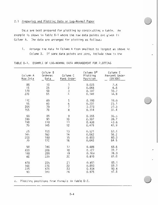
2.1 Preparing and Plottinq Data on Log-Normal Paper

Data are best prepared for plotting by constructing a table. An example is shown in Table 0-1 where the raw data points are given in Column A. The data are arranged for plotting as follows:

1. Arrange the data in Column A from smallest to largest as shown in

Column B . If some data points are zero, include them in the

TABLE D-1. EXAMPLE OF LOG-NORMAL DATA ARRANGEMENT FOR PLOTTING

Column A Raw Data

85 15 170 270

110 55 205 155

60 780 190 70

2 5 145 2 00 70

50 220 160 60

470 160 225 90

Column B Ordered Data

Column C Rank Order

1

Column Da Plotting Position

a. Plotting positions from formula in Table 0-2.

Column E Percent Under

(DXlOO)

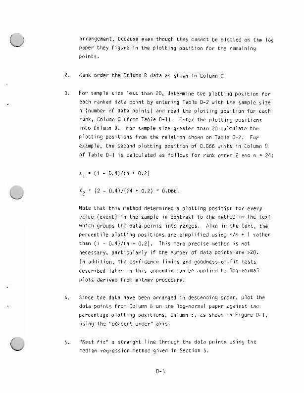
arrangement, because even though t h e y cannot be p l o t t e d on t h e l o g

paper t h e y f i g u r e i n t h e p l o t t i n g p o s i t i o n f o r t h e remain ing

Do in t s .

2. Rank o rde r t h e Column B d a t a as shown i n Column C.

3. F o r sample s i z e l e s s t han 20, determine t h e p l o t t i n g p o s i t i o n f o r

each ranked d a t a p o i n t by e n t e r i n g Tab le 0-2 w i t h t h e sample s i z e

n (number o f d a t a p o i n t s ) and read t h e p l o t t i n g p o s i t i o n f o r each

rank, Column C ( f rom Table 0-1). En te r t h e p l o t t i n g p o s i t i o n s

i n t o Column D. F o r sample s i z e g r e a t e r t han 20 c a l c u l a t e t h e

p l o t t i n g p o s i t i o n s f r om t h e r e l a t i o n shown on Table 0-2. F o r

example, t h e second p l o t t i n g p o s i t i o n o f 0.066 u n i t s i n Column 0

of Table D - 1 i s c a l c u l a t e d as f o l l o w s f o r rank o r d e r 2 and n = 24:

Note t h a t t h i s method determines a p l o t t i n g p o s i t i o n f o r eve ry

va lue (event ) i n t h e sample i n c o n t r a s t t o t h e method i n t h e t e x t

which groups t h e d a t a p o i n t s i n t o ranges. A l s o i n t h e t e x t , t h e

p e r c e n t i l e p l o t t i n g p o s i t i o n s a re s i m p l i f i e d us ing n l n + 1 r a t h e r

t han ( i - 0 .4 ) / (n t 0.2). Th i s more p r e c i s e method i s n o t

necessary, p a r t i c u l a r l y i f t h e number of d a t a p o i n t s are >20.

I n a d d i t i o n , t h e conf idence l i m i t s and goodness-of- f i t t e s t s

descr ibed l a t e r i n t h i s appendix can be app l i ed t o log-normal

p l o t s d e r i v e d f rom e i t h e r procedure.

4. Since t h e d a t a have been arranged i n descending order , p l o t t h e

da ta p o i n t s from Column 13 on t h e log-normal paper aga ins t t h e

percentage p l o t t i n g p o s i t i o n s , Column E, as shown i n F i g u r e 0-1,

us ing t h e "percent under" a x i s .

0 5. "Best f i t " a s t r a i g h t l i n e t h rough t h e da ta p o i n t s us ing t h e

median reg ress ion method g i ven i n Sec t i on 5.

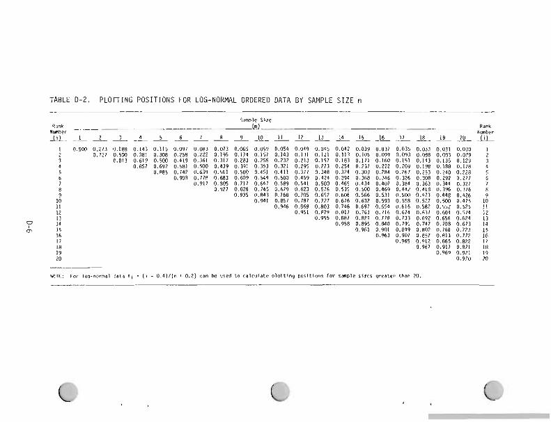
TABLE 0-2 . PLOTTING POSITIONS FOR LOG-NORMAL ORDERED DATA BY SAMPLE S I Z E n -

NOTE: For log-normal data X i = ( i

Sample s i z e In1

o.d) / [n t 0.2) can be vred t o calculate p l o t t i n g positions for ranple r i m greater than 20

-- Rank Hwber

Llil

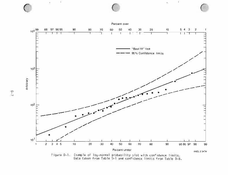
Percent over

10499 88 97 9695 90 80 70 60 50 40 30 20 10 5 4 3 2 1 - 1 1 1 1 I I I I I I I I I I l l I - - - - -

- - -

- - -

"BestfV lane - --- 95% Conftdence lhmts /- - / - /

103 =- // - - -

3 - E r - f!

- - <

D

.4 - -

- - -

- - - - - - -

, , I I

1 2 3 4 5 10 20 30 40 50 60 70 80 90 95 96 97 98 99

Percent under INEL23474

Figure D-1. Example of log-normal probability plot with confidence limits. Data taken from Table D-1 and confidence limits from Table 0-8.

6. Tes t t h e d a t a f o r randomness and homogeneity by app l y i ng t h e r u n

t e s t g i ven i n Sec t i on 6.

7. If t h e d a t a meets t h e r u n t e s t , c a l c u l a t e and p l o t t h e conf idence

l i m i t s as shown i n F i g u r e D-1, by t h e method g i v e n i n Sec t i on 7.1.

8. Make p r o b a b i l i s t i c es t ima tes from t h e log-normal d i s t r i b u t i o n

represented by t h e data :

a. The median of t h e sample d a t a i s t h e va lue a t 50% ( t h e

i n t e r s e c t i o n of t h e f i t t e d l i n e and t h e 50% l i n e ) .

b. The geometr ic d i s p e r s i o n i s t h e r a t i o o f t h e va lue a t t h e

84% l i n e t o t h e median.

c . The pe rcen t o f expected va lues under o r over a s p e c i f i e d

va lue can be read d i r e c t l y f r om t h e f i t t e d l i n e by e n t e r i n g

t h e graph a t t h e a p p r o p r i a t e percentage a x i s (pe rcen t under

o r pe rcen t ove r ) . L ikewise, t h e expected percentage of

events f a l l i n g between two s p e c i f i e d va lues can be ob ta ined

by e n t e r i n g t h e graph a t t h e s p e c i f i e d va lues on t h e f i t t e d

l i n e and s u b t r a c t i n g t h e two percentages read a t these

p o i n t s .

3. Type I ( L i n e a r ) Extreme Value D i s t r i b u t i o n s

Type I ( l i n e a r ) extreme va lue d i s t r i b u t i o n s a r e t h e r e s u l t of seve ra l

independent causes, and has found use i n s tudy ing such t h i n g s as b reak ing

loads, m e t e r o l o g i c a l and geophys ica l phenomena ( f l oods , tornados, e a r t h -

quakes, etc.) , chemical and e l e c t r i c a l p r o p e r t i e s , s tock market extremes,

and economic data. Type I extreme va lue d i s t r i b u t i o n s r e s u l t f r om systems

which can be represented by a l g e b r a i c po lynomia ls and s o l u t i o n s t o d i f f e r e n -

t i a l equat ions w i t h cons tan t c o e f f i c i e n t s . Some s a f e t y d a t a d i s t r i b u t i o n s

can be n i c e l y represented w i t h Type I extreme value.

Extreme va lue d a t a i s generated by s e l e c t i n g t h e l a r g e s t ( o r t h e

Sma l l es t ) events i n consecut ive t ime per iods , e.g., t h e l a r g e s t acc iden t

l o s s exper ienced d u r i n g consecut ive year per iods . The d i s t r i b u t i o n of

l a r g e s t va lues i s a r igh t -skewed d i s t r i b u t i o n ; t h e d i s t r i b u t i o n o f sma l l es t

values i s a lef t -skewed d i s t r i b u t i o n .

One o f t h e most use fu l p i eces of i n fo rma t i on f a l l i n g ou t o f extreme

va lue a n a l y s i s i s t h e "expected r e t u r n p e r i o d " f o r an event equal t o o r

exceeding a g i v e n s i ze .

3.1 Prepar ing and P l o t t i n g Type I Extreme Value Data

Data a re b e s t prepared f o r p l o t t i n g by c o n s t r u c t i n g a t a b l e . An

example i s shown i n Table 0-3 where t h e c o s t o f t h e l a r g e s t acc iden t of a

g i ven t ype o c c u r r i n g i n each six-month-per iod f o r e i g h t consecut ive yea rs

i s t a b u l a t e d i n Column A. The d a t a a re arranged f o r p l o t t i n g i n t h e

f o l l o w i n g s teps:

0 1. Arrange t h e d a t a i n Column A from s m a l l e s t t o l a r g e s t as shown i n

Column B.

2. Rank o r d e r Column B d a t a as shown i n Column C.

3. Determine t h e p l o t t i n g p o s i t i o n f o r each ranked d a t a p o i n t by

e n t e r i n g Table 0-4 w i t h t h e sample s i z e n (number of d a t a p o i n t s )

and read t h e p l o t t i n g p o s i t i o n f o r each rank i n Column C. E n t e r

t h e p l o t t i n g p o s i t i o n s i n t o Column D. F o r sample s i z e g r e a t e r

t han 20, c a l c u l a t e t h e p l o t t i n g p o s i t i o n s f rom t h e r e l a t i o n shown

on Tab le 0-4.

4. P l o t t h e da ta p o i n t s from Column B a t t h e p l o t t i n g p o s i t i o n s ,

Column D, on Type I ( l i n e a r ) extreme va lue graph paper

( F i g u r e 0-2). The p l o t t i n g p o s i t i o n on t h e graph paper a re on

t h e cumu la t i ve p r o b a b i l i t y ax is .

(3 5. "Best f i t " a s t r a i g h t l i n e th rough t h e d a t a p o i n t s us ing t h e

median r e g r e s s i o n method g i ven i n Sec t i on 5.

D-9

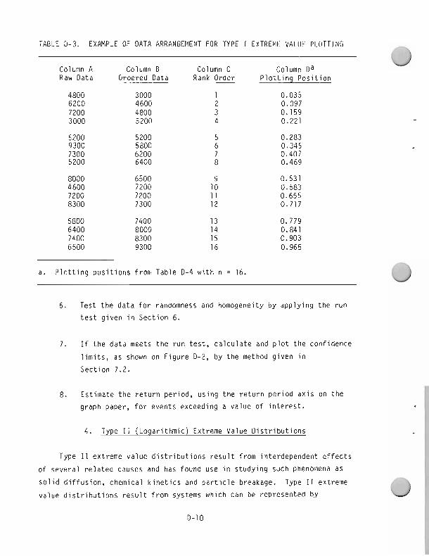
TABLE 0-3. EXAMPLE OF DATA ARRANGEMENT FOR TYPE I EXTREME VALUE PLOTTING /7

Column A Column B Column C Column Da Raw Data Ordered Data Rank Order

V P l o t t i n g P o s i t i o n

a. P l o t t i n g p o s i t i o n s f r om Table 0-4 w i t h n = 16. U 6. Test t h e d a t a f o r randomness and homogeneity by app l y i ng t h e r u n

t e s t g i v e n i n Sec t i on 6.

7 . I f t h e d a t a meets t h e r u n t e s t , c a l c u l a t e and p l o t t h e conf idence

l i m i t s , as shown on F igu re 0-2, by t h e method g i ven i n

Sec t i on 7.2.

8 . Est imate t h e r e t u r n pe r i od , us ing t h e r e t u r n p e r i o d a x i s on t h e

graph paper, f o r events exceeding a va lue o f i n t e r e s t .

4. Type I 1 (Loga r i t hm ic ) Extreme Value D i s t r i b u t i o n s

Type I 1 extreme va lue d i s t r i b u t i o n s r e s u l t f rom in terdependent e f f e c t s

o f severa l r e l a t e d causes and has found use i n s tudy ing such phenomena as I

s o l i d d i f f us ion , chemical k i n e t i c s and p a r t i c l e breakage. Type 11 extreme

va lue d i s t r i b u t i o n s r e s u l t from systems which can be represented by

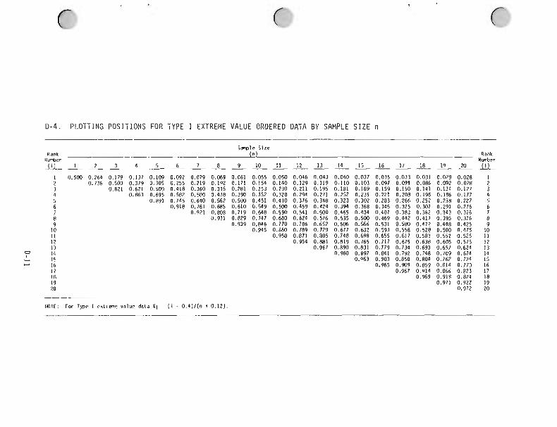
0-4. PLOTTING POSITIONS FOR

NOTE: For Tme I extreme vaiue data X i = ( i -

rYPE I EXTREME VALUE ORDERED DATA BY SAMPLE S IZE

Smple Size 0- Rank

Nunher 16 l7 I8 19 20 l i l

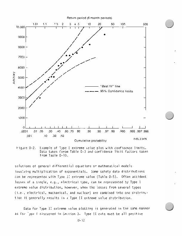
Return period (6 month periods)

i t f i t" line

Conliden,

0 1 1 I l l I I I I I I I I I I ! I I I .0001 0 1 .05 2 0 .40 6 0 7 0 .80 .90 .95 .97 .98 ,990 ,995 ,997 ,998

,001 1 0 .30 3 0 INEL23476 Cumulative probability

F i g u r e 0-2. Example of Type I extreme va lue p l o t w i t h conf idence l i m i t s . Data taken farom Table 0-3 and conf idence l i m i t f a c t o r s taken from Table 0-10.

s o l u t i o n s of genera l d i f f e r e n t i a l equat ions o r mathematical models

i n v o l v i n g m u l t i p l i c a t i o n of exponent ia ls . Some sa fe t y d a t a d i s t r i b u t i o n s

can be represented w i t h Type 11 extreme va lue (Tab le 0-5). Often acc iden t

losses of a s i n g l e , e.g., e l e c t r i c a l type, can be represented by Type I

extreme va lue d i s t r i b u t i o n , however, when t h e losses f rom severa l types

( i .e. , e l e c t r i c a l , machanical, and nuc lea r ) a re combined i n t o one d i s t r i b u -

t i o n i t g e n e r a l l y r e s u l t s i n a Type I 1 extreme va lue d i s t r i b u t i o n .

Data f o r Type I 1 extreme va lue p l o t t i n g i s generated i n t h e same manner

as f o r Type I discussed i n Sec t i on 3. Type I 1 d a t a must be a l l p o s i t i v e

0-12

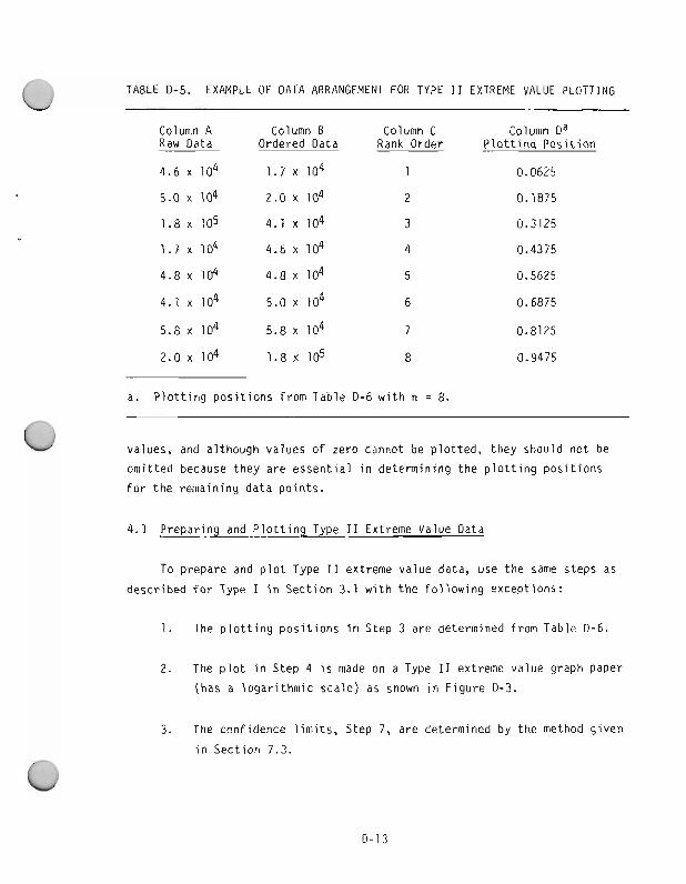
TABLE 0-5. EXAMPLE OF DATA ARRANGEMENT FOR TYPE I 1 EXTREME VALUE PLOTTINC

Column A Column B Column C Column Oa Raw Data Ordered Data Rank Order P l o t t i n g P o s i t i o n

4.6 x l o 4 1.7 x l o 4 1 0.0625

5.0 x 104 2.0 x 104 2 0.1875

1.8 105 4.1 x 104 3 0.3125

1.7 x l o4 4.6 x 104 4 0.4375

4.8 x l o 4 4.8 x lo4 5 0.5625

4.1 x l o4 5.0 x lo4 6 0.6875

5.8 x l o 4 5.8 x lo4 7 0.8125

2.0 x l o 4 1.8 x lo5 8 0.9475

a. P l o t t i n g p o s i t i o n s from Table 0-6 w i t h n = 8.

values, and al though values of zero cannot be p lo t ted , they should not be

omi t ted because they are essen t ia l i n determining the p l o t t i n g p o s i t i o n s

f o r the remaining da ta po in ts .

4.1 Preparing and P l o t t i n g Type I 1 Extreme Value Oata

To prepare and p l o t Type I 1 extreme value data, use the same steps as

described f o r Type I i n Sect ion 3.1 w i t h t h e f o l l o w i n g except ions:

1. The p l o t t i n g p o s i t i o n s i n Step 3 are determined from Table 0-6.

2. The p l o t i n Step 4 i s made on a Type I 1 extreme value graph Paper

(has a logar i thmic sca le) as shown i n F igu re 0-3.

3. The conf idence l i m i t s , Step 7, are determined by the method g iven

i n Sect ion 7.3.

0

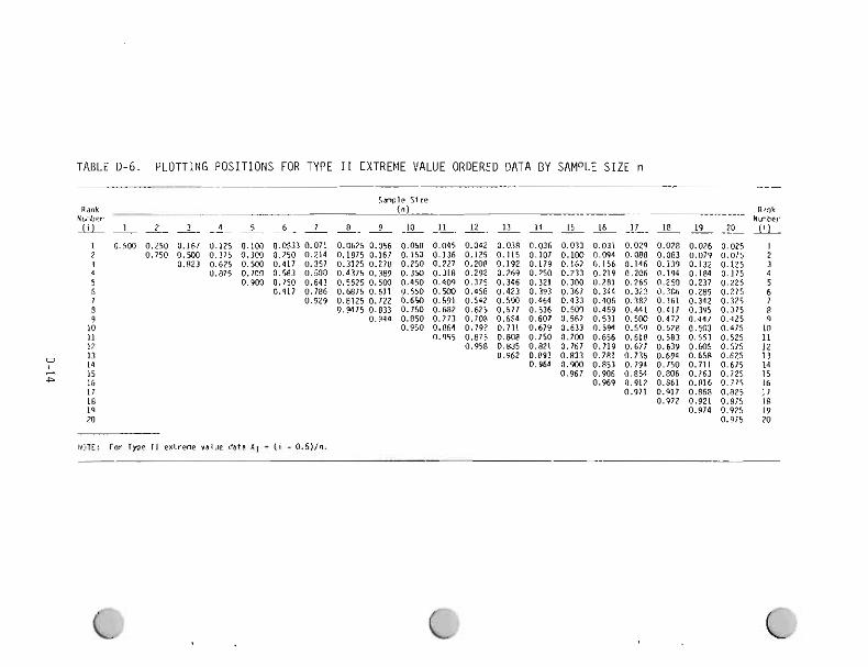
TABLE 0-6. PLOTTING POSITIONS FOR TYPE I 1 EXTREME VALUE ORDERED DATA BY SAMPLE SIZE n ----

Rank Number 1111

MTE: For Type I 1 extreme value data X i = ( 1 - 0.5)ln.

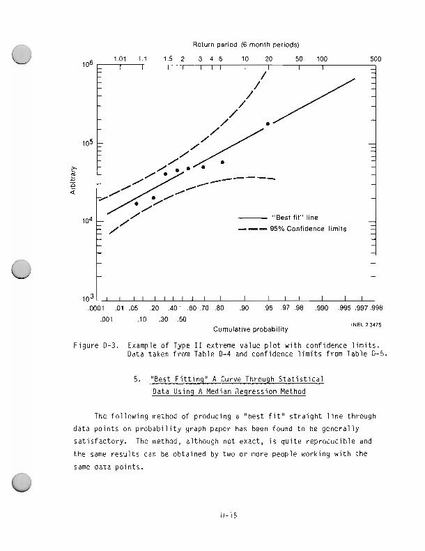
Return period (6 month periods)

I-----

// - "Best fit" line

--- 95% Confidence limits

,001 .I0 .30 S O INEL 2 3475

Cumulative probability

F igu re 0-3. Example of Type I 1 extreme value p l o t w i t h conf idence l i m i t s . Data taken f rom Table D-4 and conf idence l i m i t s from Table D-5.

5. "Best F i t t i n g " A Curve Through S t a t i s t i c a l

Data Using A Median Regression Method

The f o l l o w i n g method of producing a "best f i t " s t r a i g h t l i n e through

data p o i n t s on p r o b a b i l i t y graph paper has been found t o be genera l l y

sa t i s fac to ry . The method, al though n o t exact, i s q u i t e reproduc ib le and

the same r e s u l t s can be obtained by two o r more people working w i t h t h e

same da ta p o i n t s .

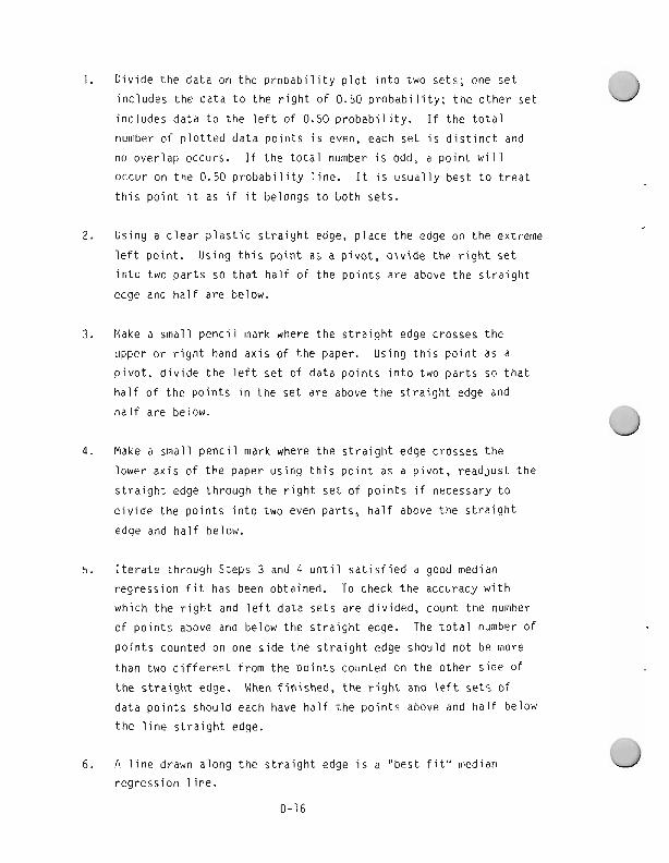
1. D i v i d e t h e da ta on t h e p r o b a b i l i t y p l o t i n t o two sets; one s e t

i nc ludes t h e d a t a t o t h e r i g h t of 0.50 p r o b a b i l i t y ; t h e o t h e r se t

i nc ludes d a t a t o t h e l e f t o f 0.50 p r o b a b i l i t y . I f t h e t o t a l

number of p l o t t e d d a t a p o i n t s i s even, each se t i s d i s t i n c t and

no ove r l ap occurs. I f t h e t o t a l number i s odd, a p o i n t w i l l

occu r on t h e 0.50 p r o b a b i l i t y l i n e . I t i s u s u a l l y bes t t o t r e a t

t h i s p o i n t it as i f it belongs t o bo th se t s .

2. Using a c l e a r p l a s t i c s t r a i g h t edge, p l a c e t h e edge on t h e extreme

l e f t po in t . Us ing t h i s p o i n t as a p i v o t , d i v i d e t h e r i g h t s e t

i n t o two p a r t s so t h a t h a l f of t h e p o i n t s a re above t h e s t r a i g h t

edge and h a l f a re below.

3. Make a smal l p e n c i l mark where t h e s t r a i g h t edge crosses t h e

upper o r r i g h t hand a x i s of t h e paper. Using t h i s p o i n t as a

p i v o t , d i v i d e t h e l e f t s e t of d a t a p o i n t s i n t o two p a r t s so t h a t

h a l f of t h e p o i n t s i n t h e se t a re above t h e s t r a i g h t edge and

h a l f a re below.

4. Make a smal l p e n c i l mark where t h e s t r a i g h t edge crosses t h e

lower a x i s of t h e paper us ing t h i s p o i n t as a p i v o t , r e a d j u s t t h e

s t r a i g h t edge th rough t h e r i g h t s e t o f p o i n t s if necessary t o

d i v i d e t h e p o i n t s i n t o two even pa r t s , h a l f above t h e s t r a i g h t

edge and h a l f below.

5. I t e r a t e t h rough Steps 3 and 4 u n t i l s a t i s f i e d a good median

reg ress ion f i t has been obtained. To check t h e accuracy w i t h

which t h e r i g h t and l e f t d a t a s e t s a re d i v i ded , count t h e number

o f p o i n t s above and below t h e s t r a i g h t edge. The t o t a l number of

p o i n t s counted on one s i d e t h e s t r a i g h t edge shou ld n o t be more

than two d i f f e r e n t f r om t h e p o i n t s counted on t h e o t h e r s i d e of

t h e s t r a i g h t edge. When f i n i shed , t h e r i g h t and l e f t s e t s of

d a t a p o i n t s shou ld each have h a l f t h e p o i n t s above and h a l f below

t h e l i n e s t r a i g h t edge.

6. A l i n e drawn a long t h e s t r a i g h t edge i s a "best f i t " median

r e g r e s s i o n l i n e .

0-16

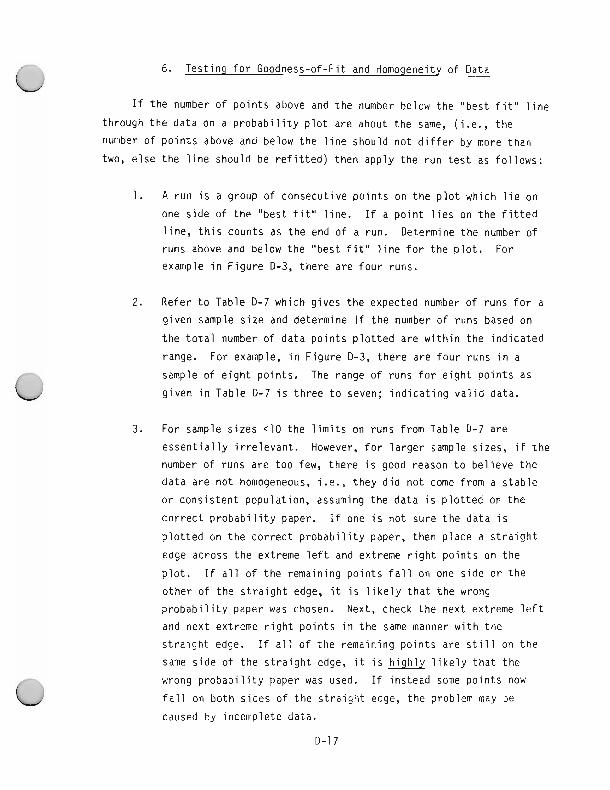
6. Tes t i ng f o r Goodness-of-Fit and Homogeneity o f Data

If t h e number of p o i n t s above and t h e number below t h e "best f i t " l i n e

th rough t h e d a t a on a p r o b a b i l i t y p l o t a re about t h e same, (i.e., t h e number of p o i n t s above and below t h e l i n e shou ld n o t d i f f e r by more t h a n

two, e l s e t h e l i n e shou ld be r e f i t t e d ) t hen app ly t h e r u n t e s t as f o l l o w s :

1. A r u n i s a group of consecut ive p o i n t s on t h e p l o t which l i e on

one s i d e o f t h e "best f i t " l i n e . I f a p o i n t l i e s on t h e f i t t e d

l i n e , t h i s counts as t h e end o f a run. Determine t h e number o f

runs above and below t h e "best f i t " l i n e f o r t h e p l o t . F o r

example i n F i g u r e 0-3, t h e r e a re f o u r runs.

2. Refer t o Tab le 0-7 which g i v e s t h e expected number o f r uns f o r a

g i v e n sample s i z e and determine if t h e number of runs based on

t h e t o t a l number of d a t a p o i n t s p l o t t e d a r e w i t h i n t h e i n d i c a t e d

range. F o r example, i n F i g u r e 0-3, t h e r e a r e f o u r runs i n a

sample of e i g h t p o i n t s . The range o f r uns f o r e i g h t p o i n t s as

g i v e n i n Table 0-7 i s t h r e e t o seven; i n d i c a t i n g v a l i d data .

3. For sample s i z e s <10 t h e l i m i t s on runs f rom Table 0-7 a re

e s s e n t i a l l y i r r e l e v a n t . However, f o r l a r g e r sample s izes , i f t h e

number of runs a re t o o few, t h e r e i s good reason t o b e l i e v e t h e

d a t a a re n o t homogeneous, i.e., t h e y d i d n o t come f rom a s t a b l e

o r c o n s i s t e n t popu la t i on , assuming t h e d a t a i s p l o t t e d on t h e

c o r r e c t p r o b a b i l i t y paper. I f one i s n o t sure t h e d a t a i s

p l o t t e d on t h e c o r r e c t p r o b a b i l i t y paper, t hen p lace a s t r a i g h t

edge across t h e extreme l e f t and extreme r i g h t p o i n t s on t h e

p l o t . I f a l l o f t h e remain ing p o i n t s f a l l on one s i d e o r t h e

o t h e r of t h e s t r a i g h t edge, i t i s l i k e l y t h a t t h e wrong

p r o b a b i l i t y paper was chosen. Next, check t h e nex t extreme l e f t

and n e x t extreme r i g h t p o i n t s i n t h e same manner w i t h t h e

s t r a i g h t edge. I f a l l o f t h e remain ing p o i n t s a r e s t i l l on t h e

same s i d e of t h e s t r a i g h t edge, i t i s l i k e l y t h a t t h e

wrong p r o b a b i l i t y paper was used. I f i ns tead some p o i n t s now

f a l l on b o t h s i des of t h e s t r a i g h t edge, t h e problem may be

caused by incomple te data .

0-17

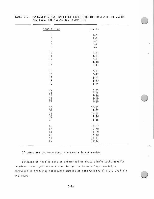
TABLE 0-7. APPROXIMATE 95% CONFIDENCE LIMITS FOR THE NUMBER OF RUNS ABOVE AND BELOW THE MEDIAN REGRESSION LINE n

Sample S i ze L i m i t s

I f t h e r e a re t o o many runs, t h e sample i s n o t random.

Evidence of i n v a l i d d a t a as determined by these s imple t e s t s u s u a l l y

r e q u i r e s i n v e s t i g a t i o n and c o r r e c t i v e a c t i o n t o e s t a b l i s h c o n d i t i o n s

conducive t o produc ing subsequent samples o f d a t a which w i l l y i e l d c r e d i b l e

es t imates .

7. Confidence L i m i t s C a l c u l a t i o n s

A f t e r a d a t a s e t has been p l o t t e d on p r o b a b i l i t y p l o t t i n g paper and a

median reg ress ion ' 'best f i t ' l i n e has been drawn th rough t h e d a t a as

descr ibed i n Sec t i on 5, conf idence l i m i t s can be de r i ved and p l o t t e d .

Examples a re shown i n F i g u r e D-1 ( log-normal p l o t ) , F i g u r e 0-2 [Type I

( l i n e a r ) extreme va lue p l o t ] and F i g u r e 0-3 [Type I1 ( l o g a r i t h m i c ) extreme

va lue p l o t ] . T h e o r e t i c a l l y , conf idence l i m i t s can be c a l c u l a t e d t o any

degree of confidence, b u t t o s i m p l i f y t h e a p p l i c a t i o n , t a b l e s o f d a t a a re

presented f o r c a l c u l a t i n g o n l y t h e 95% and 80% conf idence l e v e l . For most

d a t a p l o t t i n g a p p l i c a t i o n s , these two l e v e l s a re s a t i s f a c t o r y and use o f

t h e app rop r i a te t a b l e f a c i l i t a t e s r a p i d p l o t t i n g of t h e conf idence l e v e l

l i n e s on t h e graph. The conf idence i n t e r v a l f o r a l i n e f i t t e d t o a se t o f

d a t a po in t s , which are a sample from t h e popu la t i on , shou ld be v i s u a l i z e d

as a r e g i o n w i t h i n which t h e " t r u e " l i n e f o r t h e p o p u l a t i o n may l i e .

A l t e r n a t e l y , a conf idence i n t e r v a l may be cons idered as t h e r e g i o n w i t h i n

which t h e s p e c i f i e d percentage of a d d i t i o n a l samples w i l l r e s u l t i n f i t t e d

l i n e s w i t h i n t h e conf idence band. The l o c a t i o n o f t h e conf idence i n t e r v a l s

depend e n t i r e l y on t h e f i t t e d l i n e . The amount of s c a t t e r i n t h e p o i n t s

about t h e f i t t e d l i n e have no i n f l u e n c e whatsoever on t h e l o c a t i o n of t h e

conf idence i n t e r v a l . That i s , t h e d e v i a t i o n of conf idence l i m i t s assumes

t h e d a t a i s r e p r e s e n t a t i v e of t h e d i s t r i b u t i o n def ined by t h e f i t t e d l i n e .

As such, t h e conf idence i n t e r v a l p r o v i d e a t e s t of d a t a v a l i d i t y . For a

95% conf idence i n t e r v a l , 5% of t h e d a t a p o i n t s may l i e o u t s i d e t h e i n t e r v a l ;

f o r 30% conf idence, 20% of t h e p o i n t s may l i e o u t s i d e t h e i n t e r v a l . A

g r e a t e r t han expected percentage of p o i n t s f a l l i n g o u t s i d e t h e conf idence

i n t e r v a l suggest t h e d a t a a re n o t v a l i d ; i.e., t h e p o i n t s f a l l i n g o u t s i d e

a re n o t p a r t of t h e d i s t r i b u t i o n o r t h e e n t i r e sample may be suspect. The

source o r cause o f these p o i n t s shou ld be examined f o r d i f f e r e n c e s f rom t h e

o t h e r p o i n t s and perhaps t h e d a t a r e p l o t t e d a f t e r removing t h e "suspect "

p o i n t s .

Normally, a s u b j e c t i v e es t ima te of t h e goodness -o f - f i t i s adequate.

That i s , a good f i t i n s p i r e s a s u b j e c t i v e degree o f conf idence w h i l e w ide

s c a t t e r i n s t i l l s l e s s conf idence. For those who d e s i r e a s t a t i s t i c a l t e s t

of whether t h e l i n e f i t s a l l o f t h e data, t h i s method p rov ides such a t e s t .

7.1 Loq-Normal Conf idence L i m i t s

Log normal conf idence l i m i t s can be t a b u l a t e d and p l o t t e d as shown i n

Table 0-8 and F i g u r e 0-1. To c o n s t r u c t a conf idence l i m i t t a b l e :

1. A t t h e s e l e c t e d p e r c e n t i l e s shown i n Column A of Table D-8, t a b u l a t e as shown i n Column 8 t h e values Yp f rom t h e ' 'best f i t "

l i n e t h rough t h e p l o t t e d data . The va lues used i n t h i s example

a re t aken from F i g u r e D-1.

2. Obta in t h e a p p r o p r i a t e conf idence f a c t o r s f r om Table D-9, by i n t e r p o l a t i n g f o r t h e sample s ize, if necessary, and e n t e r t h e

f a c t o r s i n Column C. The sample s i z e n i s t h e number o f d a t a

p o i n t s used t o o b t a i n t h e "best f i t" l i n e on t h e graph. I n t h e

example, F i g u r e 0-1, n i s equal t o 24.

TABLE 0-8. EXAMPLE OF A TABLE FOR DETERMINING CONFIDENCE LIMITS ON A LOG-NORMAL PLOT

b Conf idence L i m i t s

Column A E%Y:e:ce column columns columns P rese lec ted

U p ) Fac to rs C 0 x 0

P e r c e n t i l e BID

(95%) 9 x.y U p p e r m

5 27 0.831 2.141 57.8 12.6 10 37 0.701 1.901 70.3 19.5 30 75 0.482 1.555 116.6 48.2

a. Values read from "best f i t " l i n e , F i g u r e 0-1.

b. Confidence f a c t o r s i n t e r p o l a t e d from Table 0-9.

c . g,. i s t h e r a t i o of Y0.84lYo.50 read f rom "best f i t " l i n e on F i g u r e 5 - 1 where Yo 8q and Y0,50 a re read a t t h e 84 and 50 p e r c e n t i l e s , r e s p e c t i v e l y . ~ o l u h n D i s generated by r a i s i n q q,,., t o t h e conf idence - -, ,~ f a c t o r powers f rom Column C;

D-9. CONFIDENCE FACTORS FOR THE NORMAL AND LOGARITHMIC NORMAL DISTRIBUTIONS

Conffdence Factors Preselected Percentiles - - -- - -.

30 and1310 Gnm.95 1 and 99 - 5 L 30 and 70

1.648 1.309 1.116 0 . W

0.900 0.834 0.734 0.663

0.608 0.568 0.533 0.464

0.422 0.361 0.321 0.224

1 and 99

Intermediate values may be obtained by linear interpolation.

3. Determine t h e geometr ic d i s p e r s i o n gy.x ( t h e r a t i o o f t h e

va lue on t h e "best f i t " l i n e a t t h e 84% p e r c e n t i l e and t h e 50%

p e r c e n t i l e ) . For t h e example from F i g u r e 0-2, g = Y'x

300/120 = 2.50. Raise g t o t h e power of each f a c t o r i n x.Y

Column C and e n t e r t h e r e s u l t s i n Column D, (e.g., gy.xC,

Column D).

4. M u l t i p l y each va lue i n Column B by t h e cor respond ing va lue i n

Column D t o o b t a i n p o i n t s f o r p l o t t i n g t h e upper conf idence l i m i t

curve.

5. D i v i d e each va lue i n Column 6, by t h e cor respond ing va lue i n

Column D t o o b t a i n t h e p o i n t s f o r p l o t t i n g t h e lower conf idence

l i m i t curve.

6. A t . t h e app rop r i a te p e r c e n t i l e s f rom Column A, p l o t t h e p o i n t s f o r

t h e upper and lower conf idence l i m i t curves. Draw curves th rough

t h e p o i n t s u s i n g a French o r a f l e x i b l e curve.

7.2 Type I Extreme Value ( L i n e a r ) Confidence L i m i t s

Type I extreme va lue conf idence l i m i t s can be t a b u l a t e d and p l o t t e d as

shown i n Table D-10 and F i g u r e 0-2. To c o n s t r u c t a conf idence l i m i t t a b l e :

1. A t t h e se lec ted p e r c e n t i l e s shown i n Column A of Table D-10,

t a b u l a t e i n Column 6, t h e va lues Y from t h e "best f i t" l i n e P

through t h e p l o t t e d d a t a on l i n e a r extreme va lue graph ing paper.

The Y va lues used i n t h i s example a re taken f rom F i g u r e 0-2. P

2. Obta in t h e a p p r o p r i a t e conf idence f a c t o r s f rom Table D-11, by

i n t e r p o l a t i n g f o r t h e sample s i z e i f necessary, and e n t e r t h e

f a c t o r s i n Column C. The sample s i z e n i s t h e number of d a t a

p o i n t s used t o o b t a i n t h e "best f i t " l i n e on t h e graph. I n t h e

example, F i g u r e 0-2, n i s equal t o 16.

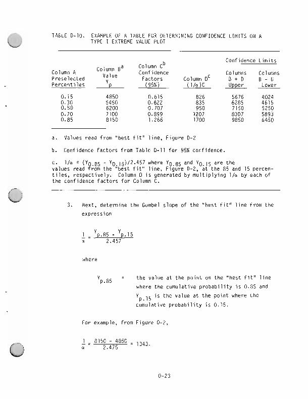
TABLE 0-10. EXAMPLE OF A TABLE FOR DETERMINING CONFIDENCE LIMITS ON A TYPE I EXTREME VALUE PLOT

b Confidence L i m i t s

Column A Coiumn B~ Value Confidence Columns Columns

P rese lec ted Fac to rs column 0' B t O B - 0 P e r c e n t i l e s Yp ( 9 % ) O / a ) C Upper Lower

a. Values read f rom "best f i t " l i n e , F i g u r e 0-2

b. Confidence f a c t o r s from Table 0-11 f o r 95% confidence.

C. l / o = (Y0.85 - Yod15)/2.457 where Y0.85 and Y0.15 a re t h e va lues read from t h e bes t fit'' l i n e , F igu re 0-2, a t t h e 85 and 15 percen- t i l e s , r e s p e c t i v e l y . Column D i s generated by m u l t i p l y i n g l / a by each of t h e conf idence f a c t o r s f o r Column C.

3. Next, de termine t h e Gumbel s l ope of t h e "best f it" l i n e from t h e

express ion

where

'p.85 = t h e va lue a t t h e p o i n t on t h e "best f i t " l i n e

where t h e cumu la t i ve p r o b a b i l i t y i s 0.85 and

Yp.15 i s t h e va lue a t t h e p o i n t where t h e

cumula t ive p r o b a b i l i t y i s 0.15.

For example, f rom F igu re 0-2,

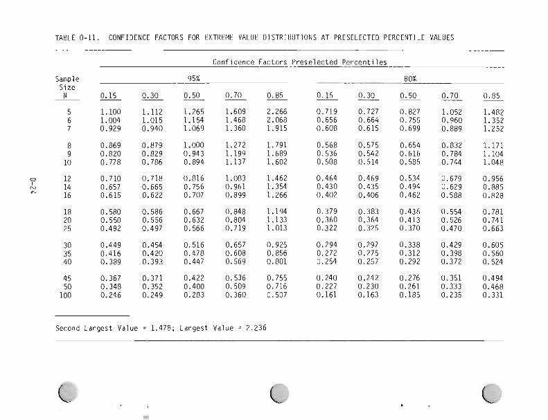
TABLE 0-11. CONFIDENCE FACTORS FOR EXTREME VALUE OISTRIBUTIONS AT PRESELECTED PERCENTILE VALUES

Sample S ize

N

5 6 7

Conf idence Fac to rs P rese lec ted P e r c e n t i l e s

95% 80%

Second La rges t Value = 1.478; La rges t Value = 2.236

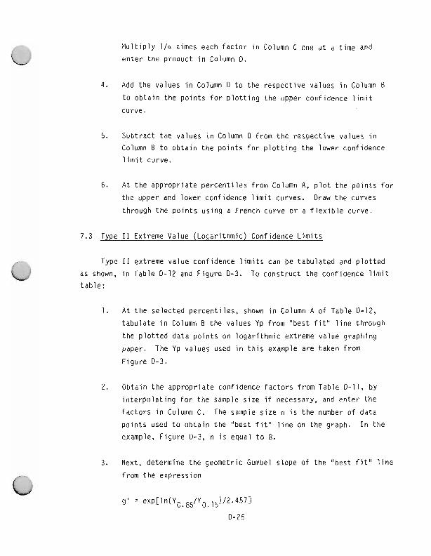
M u l t i p l y l l u t imes each f a c t o r i n Column C one a t a t ime and

en te r the product i n Column D.

4. Add t h e values i n Column 0 t o t h e respec t i ve values i n Column B

t o o b t a i n t h e p o i n t s f o r p l o t t i n g t h e upper confidence l i m i t

curve.

5. Subt ract t h e values i n Column 0 f rom t h e respec t i ve values i n

Column B t o o b t a i n t h e p o i n t s f o r p l o t t i n g t h e lower conf idence

l i m i t curve.

6 . At t h e approp r ia te p e r c e n t i l e s from Column A, p l o t t h e p o i n t s f o r

t h e upper and lower confidence l i m i t curves. Draw t h e curves

through t h e p o i n t s us ing a French curve o r a f l e x i b l e curve.

7.3 Type I 1 Extreme Value (Logar i thmic) Confidence L i m i t s

Type I 1 extreme va lue conf idence l i m i t s can be tabu la ted and p l o t t e d

as shown, i n Table 0-12 and F igu re 0-3. To cons t ruc t t h e confidence l i m i t

t a b l e :

1. A t t h e se lected pe rcen t i l es , shown i n Column A o f Table 0-12,

t a b u l a t e i n Column B t h e values Yp from "best f i t " l i n e through

t h e p l o t t e d data p o i n t s on loga r i t hm ic extreme value graphing

paper. The Yp values used i n t h i s example are taken from

F igu re 0-3.

2. Obta in t h e approp r ia te confidence f a c t o r s from Table 0-11, by

i n t e r p o l a t i n g f o r t h e sample s i z e i f necessary, and en te r t h e

f a c t o r s i n Column C. The sample s i z e n i s t h e number o f data

p o i n t s used t o o b t a i n t h e "best f it" l i n e on t h e graph. I n t h e

example, F igu re 0-3, n i s equal t o 8.

3. Next, determine t h e geometric Gumbel s lope o f t he "best f i t " l i n e

f rom t h e expression

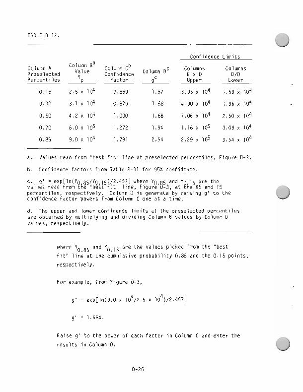
TABLE 0-12.

Confidence Limits -

column^ CO1umnBa column^ b Columns Columns Preselected Confidence DC

C B x D

Percentiles Yp Factor B/D

Upper Lower

0.15 2.5 x lo4 0.869 1.57 3.93 x lo4 1.59 x lo4 0.30 3.1 x lo4 0.879 1.58 4 . 9 0 ~ 1 0 ~ 1.96x104

0.50 4.2 x lo4 1.000 1.68 7.06 x lo4 2.50 x lo4 0.70 6.0 x 105 1.272 1.94 1.16 x lo5 3.09 x lo4 0.85 9.0 x lo4 1.791 2.54 2.29 x lo5 3.54 x lo4

a. Values read from "best fit" line at preselected percentiles, Figure 0-3.

b. Confidence factors from Table D-11 for 95% confidence.

c. g' = ex~[ln(Y~.85/Y~.l~)/2.457] where Yo. 5 and Yo 15 are the values read from the "best fit" line, Figure B-3, at the 85 and 15 percentiles, respectively. Column D is generate by raising g' to the confidence factor powers from Column C one at a time.

d. The upper and lower confidence limits at the preselected percentiles are obtained by multiplying and dividing Column B values by Column D values, respectively.

where Y 0.85 and Yo.15 are the values picked from the "best

fit" line at the cumulative probability 0.85 and the 0.15 points, respectively.

For example, from Figure 0-3,

Raise g' to the power of each factor in Column C and enter the

results in Column D.

4. M u l t i p l y t h e values i n Column 8 by t h e values i n Column 0 t o

o b t a i n t h e p o i n t s f o r p l o t t i n g the upper conf idence l i m i t curve.

5. D iv ide t h e values i n Column B by t h e values i n Column 0 t o o b t a i n

t h e p o i n t s f o r p l o t t i n g the lower conf idence l i m i t curve.

6. A t t h e appropr ia te p e r c e n t i l e s f rom Column A, p l o t t h e p o i n t s f o r

t h e upper and lower conf idence l i m i t curves. Draw curves through

t h e p o i n t s us ing a French curve o r a f l e x i b l e curve.

8. References

1. " P r o b a b i l i t y Charts f o r Dec is ion Making," J. R. King, I n d u s t r i a l

Press Inc., 200 Madison Avenue, New York, NY 10016, ( L i b r a r y o f

Congress Catalog Card Number 76-112966).

2. TEAM Easy Analys is Methods, Vol. 4, No. 1, 1977.

3. I b i d , Yol. 5 No. 1, 1978.

4. I b i d , Vol. 6No . 1, 1979.

5. I b id , Vol. 6 No. 2, 1979.

6. I b i d , Vol. 6 No. 3, 1979.

7. I b i d , Vol. 6 No. 4, 1979.

8. E. J. Gumbel, " S t a t i s t i c a l Theory o f Extreme Values and Some

P r a c t i c a l Appl icat ions, " February 1954, Na t iona l Bureau of

Standards Appl ied Mathematics Series, 33.

NOTE: TEAM Easy Analys is Methods p u b l i c a t i o n s a re a v a i l a b l e from TEAM,

Box 25, Tamworth, NH 03886, Telephone 603-323-8843.

APPENDIX E

R I S K ASSESSMENT EXAMPLES

This page intentionally blank

APPENDIX E

RISK ASSESSMENT EXAMPLES

1. L o g i s t i c s P r o b a b i l i t y and R i s k Assoc ia ted

Wi th a Reactor ~ e f l e c t o r ~

Apparent ly t h e d e c i s i o n t o s h i p t h e l a t e s t replacement r e f l e c t o r on

f i v e separa te t r u c k s was based on an a n a l y s i s made by an AEC s t a t i s t i c i a n .

Al though we agree t h a t t h e r e l a t i v e r i s k i s reduced by t h i s means, we a re

n o t convinced t h a t t h e r e d u c t i o n i n abso lu te r i s k i s wo r th t h e increased

cost .

A t tached i s a new s tudy performed on t h e p r o b a b i l i t i e s o f cargo damag-

i n g acc iden ts and assoc ia ted r i s k s of sh ipp ing t h e r e f l e c t o r f rom t h e manu-

f a c t u r e r , American B e r y l l i u m Company, Sarasota, F l o r i d a . The r e s u l t s a re

b r i e f l y summarized f o r an opt imized shipment ( i .e. , s e l e c t i o n o f t h e b e s t

t r u c k s i n t h e f l e e t ; s e l e c t i o n of t h e bes t d r i v e r s ; s e l e c t i o n o f t h e b e s t

rou te , w i t h an op t im ized d r i v i n g schedule and t r u c k spacing t o avo id a cas-

cad ing acc iden t ) . R i sk i s t h e d o l l a r va lue t imes t h e p r o b a b i l i t y o f l oss .

1. The shipment cou ld be make on one t r u c k w i t h a cargo damage p r o -

b a b i l i t y o f 7 x The l o s s of cargo r i s k i s $466. The l o s s

of r e a c t o r o p e r a t i o n r i s k i s $5250.

2. The shipment can be made by t r a n s p o r t i n g t h e 10 r e f l e c t o r p ieces

i n d i s s i m i l a r p a i r s w i t h a p a i r on each of f i v e t r ucks . The cargo

damage r i s k i s e s s e n t i a l l y t h e same as f o r sh ipp ing a l l t h e pack-

ages on one t r u c k . The r i s k f rom l o s s o f r e a c t o r ope ra t i on i s

reduced t o $37. Th i s r i s k does n o t i n c l u d e a f a c t o r f o r

programmatic d i s r u p t i o n .

3. If no s e l e c t i o n process i s invo lved, t o improve acc ident probab i -

l i t i e s over t h e average f o r t r u c k shipments, these r i s k s cou ld be

expected t o increase by a t l e a s t a f a c t o r o f 10.

a. Th i s a n a l y s i s i s taken from a l e t t e r which has been d i sgu i sed t o conceal i t s o r i g i n .

I n ou r op in i on , if t h e r i s k i n v o l v e d i n sh ipp ing v i a f i v e t r u c k s r a t h e r

t h a n one t r u c k i s weighed aga ins t t h e increased s h i p p i n g cos t , i t i s p rob-

a b l y no t wo r th t h e added c o s t t o make a f i v e - t r u c k shipment. However, t h e

cus tomer ' s wishes and w i l l i n g n e s s t o u n d e r w r i t e t h e c o s t o f t h e i nc remen ta l

r e d u c t i o n (about $5200) i n r i s k must a l s o be cons idered.

1.1 Statement o f Problem

Ten b e r y l l i u m r e f l e c t o r p ieces , f i v e of each type, a re t o be shipped

v i a t r u c k f r om t h e f a b r i c a t o r ' s shop t o t h e r e a c t o r s i t e . I f an acc iden t

occurs, which p reven ts t h e r e c e i p t o f f o u r undamaged l i k e s e t s o f p ieces ,

r e a c t o r o p e r a t i o n c o u l d be de layed a t cons ide rab le c o s t . I t i s proposed t o

s h i p t h e p i eces on f i v e separa te t r u c k s , i n packages o f two d i s s i m i l a r

p i eces p e r package. How much i s t h e p r o b a b i l i t y o f success fu l shipment of

a t l e a s t f o u r s e t s o f p i eces improved by t h i s method ove r s h i p p i n g a l l of

t h e p i eces on one t r u c k ?

1 . 2 Assumptions

I. The p r o b a b i l i t y o f a cargo damaging acc iden t i s equal f o r a l l

t r u c k s . T h i s assumes t h e t r u c k s are i n equal o p e r a t i n g c o n d i t i o n ,

d r i v e n by d r i v e r s of equa l s k i l l w i t h e q u i v a l e n t d r i v i n g records ,

over t h e same rou te .

2. A l l f a i l u r e events ( ca rgo damaging a c c i d e n t ) and independent.

(Trucks a re spaced s u f f i c i e n t l y t o e l i m i n a t e a cascad ing acc iden t

i n v o l v i n g more t h a n one t r uck . )

1.3 S o l u t i o n

The b inom ia l law s t a t e s : If t h e p r o b a b i l i t y of occur rence of an event

i n a s i n g l e t r i a l i s p, t hen t h e p r o b a b i l i t y t h a t i t w i l l occur exactly r t imes i n n independent t r i a l s i s

where

n! C = n r r!(n - r)!

This law can be extended to state: If the probability of the

occurrence of an event on a single trial is p, then the probability that

the event will occur at least r times in the course of n independent trials

is

r n-r + . . . + nCn-rP (1 - P) .

For our case the n independent trials are the five truck trips and the

events r are cargo damaging accidents. Since two or more truck accidents

are required to "fail the system" and delay reactor operation, the above

eauation reduces to

This function was calculated for various values of p, the probability

of a single truck having a cargo damaging accident (failure) and are tabulated below.

Inspection of the table reveals facts which may not be intuitively

obvious about this type logistic problem. If the probability of a truck

accident is large, the probability of system failure (two or more accidents

occurring in the five trials) is actually increased. Only when the single

accident event probability is small is there an improvement in success

probability.

This suggests that every effort should be made to reduce the value of

p, the probability of a single truck accident while traveling the route.

This reduction is best accomplished by selecting the best trucks in

the fleet, as demonstrated by inspection; selection of the best drivers

with the best driving records; selection of the safest route with truck

movement at controlled speed allowed only during the safest period of the

day. It is expected that at least a factor of 10 improvement in safety

could be realized over the average.

I f the probability of a single truck accident can be reduced suffi-

ciently, it then becomes important to look at the economics of shipping via

five trucks or one truck. Is the probability of an accident so small, that

the added cost of shipping the reflector on five trucks is justified?

Tri-State trucking statistics reveal that from 1964 to 1972, 3 million

vehicle miles were traveled, and only one accident occurred which could be

considered cargo damaging. It is assumed that the beryllium packages will

be well constructed and properly tied down. Tri-State data should be

characteristic of probabilities for well regulated shipments; i.e., the

extra mile for safety. (Reference 1 gives 3 x 10-~/vm for moderate accident frequency and 8 x 10-~/vm vor severe accident frequency.)

Using the Tri-State frequency of 3 x cargo damaging accidents 7 per vehicle mile, the probability of the undesired event p is (3 x 10- ) x

2400 miles (the shipment is to originate in Sarasota, Florida) or 7 x 10.~.

There is about one chance in 1400 of having a cargo damaging accident. By sending the packages on five trucks, the probability of at least two cargo

damaging accidents is 5 x roughly a two order of magnitude improve- ment for system success over sending all the packages on one truck.

Risk is the loss due to an undesirable event times the probability of

that event occurring. The risk to the cargo, where the cargo is $666K worth

of machined beryllium, is the same whether shipped via one truck or

one-fifth of the cargo on each of five trucks. The risk, however, is

distributed differently, since with five trucks there is nearly five times

the probability of losing one cargo package, a small probability of losing

two packages, and virtually no probability of losing more that two

packages. These probabilities calculated using the binomial law and a

value of 7 x for p is tabulated below to illustrate this distribution.

Exactly 0 loss out of 5 0.9965

Exactly 1 loss out of 5 0.0034902

Exactly 2 losses out of 5 4.89 x

Exactly 3 losses out of 5 3.43 x 1Wg

Exactly 4 losses out of 5 1.20 x 10-I?

Exactly 5 losses out of 5 1.68 x 10-l6

The total cargo loss risk for the beryllium is thus $466.

The risk of keeping the reactor off-line due to loss of two or more packages based on a 125K per day operating cost and a 10-month part

replacement lead time is:

1. F i v e packages on one truck--$25,00O/day x 300 days x 7 X 1 0 ' ~ :

$5250

2. F i v e packages on f i v e trucks--$25,000/day x 300 days x 4.89 x

= 637 ( r e q u i r e s two o r more package l osses ) .

These are a c t u a l l y t h e minimum r i s k s , s i nce no f a c t o r f o r programmatic

d i s r u p t i o n i s inc luded. The 10-month replacement t ime i s based on t h e

l e n g t h o f t h e p resen t f a b r i c a t i o n and t e s t c o n t r a c t . I t i s assumed t h e

b e r y l l i u m i s n o t dest royed i n an acc ident , so t h e damaged m a t e r i a l cou ld be

remelted, cas t , and machined i n t o t h e r e q u i r e d r e f l e c t o r s (i.e., i t i s n o t

necessary t o f i n d an a d a i t i o n a l source of h igh-grade b e r y l l i u m ) .

2. Reference

A r t i c l e i n t h e NUCLEAR NEWS dated May 1973, e n t i t l e d "T ranspo r ta t i on

Acc idents : How Probable?", by W i l l i a m A. Brobst.

3. R i sk From A i r c r a f t

t o a New Support B u i l d i n g A d d i t i o n

3.1 Summary

The proposed a d d i t i o n t o t h e new suppor t b u i l d i n g , w i t h a c a p a c i t y of

500 personnel , w i l l be l o c a t e near t h e south end of t h e secondary runway.

Approx imate ly 20,000 l and ings o r takeof fs pe r year , us ing t h e south end of

t h i s runway, r e s u l t i n f l i g h t pa ths near t h e proposed b u i l d i n g . The proba-

b i l i t i e s o f an a i r c r a f t impac t i ng t h e b u i l d i n g and t h e assoc ia ted r i s k s a re

g i ven i n Table E-1.

If t h e e x i s t i n g b u i l d i n g s a re a l s o considered, t h e va lues i n Table E-1,

w i t h t h e excep t i on of t h e i n d i v i d u a l r i s k value, a re approx imate ly doubled.

The i n d i v i d u a l r i s k remains approx imate ly t h e same. The bes t es t ima te

values are approx imate ly equ i va len t t o a b u i l d i n g impact o f 1 i n 12,000

years , a f a t a l i t y r i s k o f 1 i n 1200 years, and an i n d i v i d u a l f a t a l i t y r i s k

o f 1 i n 600,000 years . The worst-case es t imates a re equ i va len t t o a company

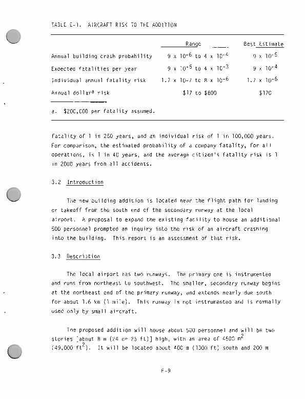
TABLE E-1. AIRCRAFT RISK TO THE ADDITION

Range Best Est imate

Annual b u i l d i n g c rash p r o b a b i l i t y 9 x 10-6 t o 4 x 10-4 9 x 10-5

Expected f a t a l i t i e s pe r yea r 9 x l o - s t o 4 x 10-3 9 x lo -q

I n d i v i d u a l annual f a t a l i t y r i s k 1.7 x 10-7 t o 8 x 10-6 1.7 x 10-6

Annual d o l l a r a r i s k $17 t o $800 $170

a. $200,000 pe r f a t a l i t y assumed.

f a t a l i t y of 1 i n 250 years, and an i n d i v i d u a l r i s k of 1 i n 100,000 years .

For comparison, t h e es t imated p r o b a b i l i t y of a company f a t a l i t y , f o r a l l

opera t ions , i s 1 i n 40 years, and t h e average c i t i z e n ' s f a t a l i t y r i s k i s 1

i n 2000 years from a l l acc idents .

3.2 I n t r o d u c t i o n

The new b u i l d i n g a d d i t i o n i s l oca ted near t h e f l i g h t p a t h f o r l and ing

o r t akeo f f f r om t h e south end o f t h e secondary runway a t t h e l o c a l

a i r p o r t . A p roposa l t o expand t h e e x i s t i n g f a c i l i t y t o house an a d d i t i o n a l

500 personnel prompted an i n q u i r y i n t o t h e r i s k of an a i r c r a f t c rash ing

i n t o t h e b u i l d i n g . Th i s r e p o r t i s an assessment o f t h a t r i s k .

3.3 D e s c r i p t i o n

The l o c a l a i r p o r t has two runways. The p r i m a r y one i s ins t rumented

and runs f rom no r theas t t o southwest. The smal le r , secondary runway beg ins

a t t h e no r theas t end o f t h e p r i m a r y runway, and extends n e a r l y due south

f o r about 1.6 km ( 1 m i l e ) . T h i s runway i s n o t ins t rumented and i s no rma l l y

used o n l y by smal l a i r c r a f t .

The proposed a d d i t i o n w i l l house about 500 personnel and w i l l be two

s t o r i e s [about 8 m (24 o r 25 f t ) ] h igh, w i t h an area of 4500 rn2 2 (49,000 ft ) . I t w i l l be l o c a t e d about 400 m (1300 f t ) south and 200 m

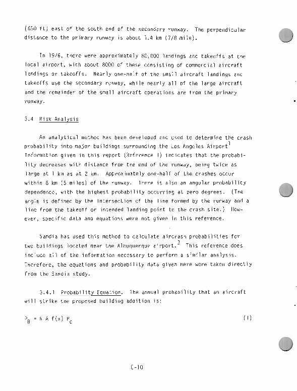
( 650 ft) east of the south end of the secondary runway. The perpendicular distance to the primary runway is about 1.4 km (718 mile).

In 1976, there were approximately 80,000 landings and takeoffs at the

local airport, with about 8000 of these consisting of commercial aircraft

landings or takeoffs. Nearly one-half of the small aircraft landings and

takeoffs use the secondary runway, while nearly all of the large aircraft

and the remainder of the small aircraft operations are from the primary

runwav.

3.4 Risk Analysis

An analytical method has been developed and used to determine the crash

probability into major buildings surrounding the Los Angeles Airport 1

Information given in this report (Reference I) indicates that the probabi-

lity decreases with distance from the end of the runway, being twice as

large at 1 km as at 2 km. Approximately one-half of the crashes occur

within 8 km (5 miles) of the runway. There is also an angular probability

dependence, with the highest probability occurring at zero degrees. (The

angle is defined by the intersection of the line formed by the runway and a

line from the takeoff or intended landing point to the crash site.) How-

ever, specific data and equations were not given in this reference.

Sandia has used this method to calculate aircrash probabilities for

two buildings located near the Albuquerque a i r ~ o r t . ~ This reference does

include all of the information necessary to perform a similar analysis.

Therefore, the equations and probability data given here were taken directly

from the Sandia study.

3.4.1 Probability Equation. The annual probability that an aircraft

will strike the proposed building addition is:

where

N = t h e number o f o p e r a t i o n s l y r

A 2 = t h e e f f e c t i v e b u i l d i n g area (km )

f ( x ) = a d i s t r i b u t i o n f u n c t i o n f o r c rash p r o b a b i l i t y ( p e r km)

= p r o b a b i l i t y of c rash pe r km o f f l i g h t .

A summation equat ion i s g i ven i n Reference 2, which must be used i f

d i f f e r e n t t ypes of a i r c r a f t , o r d i f f e r e n t modes o f opera t ion , o r more than

one f l i g h t p a t h a re considered. S ince we a re cons ide r i ng o n l y t h e south

approach t o t h e secondary runway and o n l y genera l a v i a t i o n (which has equal

c r a s h p r o b a b i l i t i e s f o r t a k e o f f s and land ings) , t h e summation i s n o t needed.

(The i n f l i g h t mode i s neg lec ted because of t h e lower c rash p r o b a b i l i t y and

lower number of f l i g h t s near t h e b u i l d i n g . )

3.4.2 A i r T r a f f i c . One-fourth o f t h e 80,000 land ings and takeof fs

a r e assumed t o use t h e south end o f t h e secondary runway. A l l o f these

20,000 ope ra t i ons a re assumed t o be general a v i a t i o n a i r c r a f t . The o t h e r

Operat ions a re neg lec ted because t h e y do n o t occur near t h e proposed

f a c i l i t y . Therefore, N = 20,000 ope ra t i ons l yea r .

3.4.3 E f f e c t i v e B u i l d i n g Area. The e f f e c t i v e b u i l d i n g area i s t h e 2 2 roo f area of 4500 m (49,000 f t ), p l u s a "shadow" area of 1500 m 2

2 (14,600 ft ) de f i ned by an assumed g l i d e ang le o f 20 degrees, a b u i l d i n g

h e i g h t of 8 m (25 f t ) , and a w i d t h of 70 m (230 f t ) . Th i s g i ves a t o t a l 2 2 area of 0.006 km (63,600 f t ) . A " s k i d " area, d e f i n e d as t h e w i d t h o f

t h e b u i l d i n g m u l t i p l i e d by t h e average s k i d l e n g t h o f 100 m (328 f t ) o r 2 2 0.007 km (7200 f t ) f o r genera l a v i a t i o n a i r c r a f t i s om i t t ed because

t h e k i n e t i c energy would be r a p i d l y d i s s i p a t e d so t h a t t h e consequence of a

l i g h t p l ane s k i d d i n g i n t o a b u i l d i n g , on t h e average, would be much l e s s

t han t h a t f rom a d i r e c t s t r i k e above ground l e v e l . Therefore,

A = 0.006 km2.

3.4.4 Impact Distribution. Crash probabilities are given for three

different modes of flight: landing, takeoff, and inflight. (Landing and

takeoff are defined as any operation within 8 km of the airport.) The

inflight probabilities are considered constant for a given type of aircraft,

but probabilities for the other two modes must be modified by a distribution function, which is the same for both modes and is given by:

where

x = the perpendicular distance from the intended flight path

to the new flight path to the new facility (0.2 km)

5 3.4.5 Crash Probability. The crash probabilities per 10 km of

flight, for different classes of general aviation, range from 0.095 to 0.26

for landing, and from 0.063 to 0.39 for takeoffs. However, these probabi-

lities, averaged for all general aviation flights, are equal for takeoffs 5 and landings, at 0.15 per 10 km. (Aircarrier crash probabilities are

only 0.007 for takeoffs and 0.028 for landings.) Since the general aviation

average is within approximately a factor of two of the specific values, it

is used without attempting to determine the numbers of flights for the dif-

ferent types (charter, pleasure, etc.) within the general aviation category. -6 Therefore, P C = 1.5 x 10 /km.

3.4.6 Probability of Building Impact. Using Equation (1) and the

above input values, the probability of building impact is:

PB = 8.6 x impacts lyear .

T h i s i s approx imate ly e q u i v a l e n t t o one impact i n 12,000 yea rs ( o r one

i n 6000 years if s k i d d i n g i n t o t h e b u i l d i n g i s i nc luded ) .

3.4.7 Consequences. Reference 1 g i ves a d e s t r u c t i o n c o e f f i c i e n t o f

0.06 f o r l i g h t a i r c r a f t impact i n t o t h e average o f f i c e b u i l d i n g . T h i s means

t h a t 6% o f t h e persons i n t h e average b u i l d i n g would be k i l l e d . However, i t appears t h a t t h e pe rcen t of t h e occupants s u f f e r i n g a f a t a l i t y would n o t

be a cons tan t 6%. b u t would be sma l l e r f o r l a r g e r o f f i c e b u i l d i n g s . A con-

sensus o f severa l eng ineers i s t h a t no more than severa l o f f i c e s i n t h e

b u i l d i n g would be destroyed, and t h a t 10 f a t a l i t i e s i s a reasonab le e s t i -

mate. I n j u r i e s and p r o p e r t y damage a re smal l by comparison. W i th an

assumed va lue of $200,000 p e r f a t a l i t y , t h e consequence o f a l i g h t a . i r c r a f t

s t r i k i n g t h e b u i l d i n g i s es t imated a t 10 f a t a l i t i e s o r approx imate ly

$2,000,000.

3.4.8 s. Risk can be thought o f as t h e amount o f insurance which

w i l l cover expected losses, and i s de f i ned as t h e consequence o f an event

m u l t i p l i e d by i t s p r o b a b i l i t y of occurrence:

5 R i s k = PBC = (8 .6 x 10- ) ( 1 0 f a t a l i t i e s o r $2,000,000)

= 8.6 x f a t a l i t i e s j y e a r o r ~ l ~ y e a r .

The f a t a l i t y r a t e i s equ i va len t t o about one f a t a l i t y i n 1200 years .

W i th 500 personnel i n t h e b u i l d i n g , t h e annual i n d i v i d u a l r i s k i s o n l y one

i n 600,000. If t h e p r o b a b i l i t y o f s k i d d i n g i n t o t h e b u i l d i n g i s inc luded,

t h e r i s k es t ima te i s increased, b u t n o t doubled, because t h e consequence

would be much l e s s t han 10 f a t a l i t i e s . Also, i f t h e e x i s t i n g b u i l d i n g s and

Personnel a re included, t h e company r i s k i s doubled, b u t t h e i n d i v i d u a l

Person 's r i s k remains t h e same, s i nce t h e t o t a l f a t a l i t y r i s k i s shared by

t w i c e as many persons. I n comparison, a company acc iden t f a t a l i t y i s

expected once i n 40 years, and an i n d i v i d u a l employee's chance pe r yea r o f

a f a t a l occupat iona l acc iden t i s one i n 120,000 years.

3.5 D iscuss ion and Conc lus ion

The above r i s k va lues a re considered b e s t es t imates . To determine t h e

degree of unce r ta in t y , a worst-case was c a l c u l a t e d us ing t h e f o l l o w i n g

conse rva t i ve a s s u m ~ t i o n s :

1. The a i r t r a f f i c i s p r o j e c t e d t o increase by 50%.

2. A g l i d e ang le of 10 degrees r a t h e r t han 20 degrees i s assumed.

T h i s increases t h e shadow area by a f a c t o r o f two and t h e b u i l d -

i n g ( t a r g e t ) area by 23%. Adding t h e s k i d area, b u t compensating

f o r t h e l e s s severe consequences of a s k i d d i n g c o l l i s i o n g i ves an

es t imated 50% increase i n r i s k .

3. The f l i g h t p a t h i s 120 m (400 f t ) , r a t h e r t han 200 m (650 f t )

f rom t h e b u i l d i n g . Th i s increases t h e d i s t r i b u t i o n f u n c t i o n t o

0.53 f rom 0.48, a 10% increase.

4. A i r c r a f t f rom t h e p r imary runway a re inc luded. Th i s does n o t

double t h e r i s k because t h e d i s t r i b u t i o n f u n c t i o n i s o n l y 0.11

vs. 0.48 f o r t h e secondary runway. Adding 0.11 t o 0.48 g i ves an

i nc rease o f 23%. (Note t h a t t h e b u i l d i n g i s n o t l oca ted near t h e

a i r p a t h d u r i n g t a k e o f f o r land ing, bu t i s about 1.5 km perpend i -

c u l a r t o t h e c e n t e r p o r t i o n o f t h e p r imary runway. The d i s t r i b u -

t i o n f u n c t i o n i s t hus probab ly s t r o n g l y conse rva t i ve i n t h i s

ins tance. A l so no te t h a t c o n s i d e r a t i o n of l a r g e a i r c r a f t leads

t o no change i n r i s k es t imate . A i r c a r r i e r c rash p r o b a b i l i t y i s

approx imate ly 1/10 o f t h a t o f genera l a v i a t i o n , b u t t h e conse-

quences a re p robab l y 10 t imes as severe.)

5 5. The mean takeof f and l and ing crash p r o b a b i l i t i e s pe r 10 km f o r

genera l a v i a t i o n are : i ns t ruc t i ona l - -0 .08 ; business--0.09;

pleasure--0.32; a e r i a l app l ica t ion- -0 .13; a i r t ax i - -0 .08 . There-

f o r e , a d i s p r o p o r t i o n a t e number o f p l easu re c r a f t us ing t h e

secondary runway, compared t o t h e n a t i o n a l average would i nc rease

t h e c rash p r o b a b i l i t y above t h e 0.15 n a t i o n a l average. Since it

i s known t h a t n o t a l l a i r c r a f t a t t h e f i e l d a re p leasu re c r a f t ,

t h e worst-case i s es t imated t o be a 50% increase i n r i s k .

When t h e above f a c t o r s a re compounded, t h e worst-case r i s k i s app rox i -

mate ly 4.5 t imes as g r e a t as t h e c a l c u l a t e d "bes t es t ima te " value. On t h e

o t h e r hand, t h e f o l l o w i n g conservat isms were n o t i nc luded i n t h e "bes t

es t ima te " c a l c u l a t i o n :

1. No c r e d i t was taken f o r s h i e l d i n g of t h e f a c i l i t y by o t h e r b u i l d -

ings . (There a re severa l l a r g e b u i l d i n g s l oca ted between t h e

runway and t h e new f a c i l i t y . )

2. No c r e d i t was taken f o r evas ive ac t i on . (A p i l o t w i l l a t tempt t o

avo id a s t r u c t u r e . )

3 . The o f f i c e b u i l d i n g i s occupied o n l y 8 hours p e r day, 5 days pe r

week.

4. A l l ope ra t i ons us ing t h e secondary runway a re under v i s u a l f l i g h t

r u l es , w h i l e those ope ra t i ons under i ns t rumen t f l i g h t r u l e s

l i k e l y have a h i g h e r c rash p r o b a b i l i t y .

A s u b j e c t i v e es t imate , cons ide r i ng t h e above conse rva t i ve f a c t o r s and

o p t i m i s t i c ( r a t h e r than worst-case) i n p u t parameters i s t h a t t h e r i s k s a re

about a f a c t o r o f 10 l e s s than t h e bes t es t ima te values.

The r e s u l t i n g o p t i m i s t i c es t imates , and t h e worst-case values, d e f i n e

t h e ranges of u n c e r t a i n t y i n t h e r i s k . These ranges a re g i ven i n Table E-1,

t o g e t h e r w i t h t h e bes t es t ima te values.

4. References

1. D. K. Okrent, " A i r p l a n e Crash R isk t o Ground Popu la t ion , " Hazard

Prevent ion , 11, 3 (January lFebruary 1975).

2. B e t t y B i r i n g e r , "Assessment o f t h e P r o b a b i l i t i e s o f A i r c r a f t Impact

w i t h t h e Sandia Pulsed Reactor and B u i l d i n g 836, Sandia Labo ra to r i es ,

A1 buquerque," SAND76-0366, November 1976.

E-15