Embed Size (px)
Citation preview

University of Nebraska - LincolnDigitalCommons@University of Nebraska - Lincoln
Journal of Actuarial Practice 1993-2006 Finance Department
1998
Actuarial Techniques in Risk Pricing and CashFlow Analysis for U.K. Bank LoansPhilip BoothCity University, [email protected]
Duncan E.P. WalshCity University, [email protected]
Follow this and additional works at: http://digitalcommons.unl.edu/joap
Part of the Accounting Commons, Business Administration, Management, and OperationsCommons, Corporate Finance Commons, Finance and Financial Management Commons, InsuranceCommons, and the Management Sciences and Quantitative Methods Commons
This Article is brought to you for free and open access by the Finance Department at DigitalCommons@University of Nebraska - Lincoln. It has beenaccepted for inclusion in Journal of Actuarial Practice 1993-2006 by an authorized administrator of DigitalCommons@University of Nebraska -Lincoln.
Booth, Philip and Walsh, Duncan E.P., "Actuarial Techniques in Risk Pricing and Cash Flow Analysis for U.K. Bank Loans" (1998).Journal of Actuarial Practice 1993-2006. 89.http://digitalcommons.unl.edu/joap/89

Journal of Actuarial Practice Vol. 6, 1998
Actuarial Techniques in Risk Pricing and Cash Flow Analysis for U.K. Bank Loans
Philip Booth* and Duncan E.P. Walsh t
Abstract*
A cash flow model is developed to set the price for a loan to a borrower with known risks. Similarities are noted between this model and those used for profit testing in life insurance. We emphasize aspects that reasonably can be treated in several ways and also indicate where the cash flow model differs from the pricing methods usually employed in bank lending. The sensitivity of interest rates to various parameters of the model such as the length of loan and the expected default rate is examined. Also, we examine how features of loans, including cash back and early repayments, can be priced.
Key words and phrases: credit risk, default rate, equity, expenses, mortgages, net present value
*Philip Booth is a senior lecturer in actuarial science at City University. He has previously worked in the investment department at Axa Equity and Law and has taught in Eastern Europe. He is the co-author of two books and a number of papers in actuarial SCience. Mr. Booth is an assistant editor of the British Actuarial Journal and is a member of a number of Institute of Actuaries' Committees.
Mr. Booth's address is: Department of Actuarial Science and Statistics, City University, Northampton Square, London ECIV OHB, ENGLAND. Internet address: [email protected]
tDuncan E.P. Walsh, Ph.D., is a researcher in actuarial science at City University. He joined the department in 1996 after completing a Diploma in Actuarial Science at City University. Dr. Walsh obtained his bachelor's degree in mathematics and astronomy from the University of Leicester, England, and his Ph.D. in astrophysical sciences from Princeton University, USA. He was an astrophysicist, focusing on cosmology, serving as a researcher at Cambridge University (England) and at Hokkaido University (Japan). His current research interests include long-term care and property investments.
Dr. Walsh's address is: Department of Actuarial SCience and Statistics, City University, Northampton Square, London ECIV OHB, ENGLAND. Internet address: [email protected]
*This paper is based on a previous paper entitled "An Actuarial Approach to the Pricing of Banking Risk" in Proceedings of the 1997 Faculty and Institute of Actuaries Investment Conference, Faculty and Institute of Actuaries, 1998 (forthcoming). The authors wish to thank the following: lain Allan for helpful comments and practical guidance, the Institute of Actuaries and the Royal Bank of Scotland for funding of research grants, the anonymous referees, and the editor for their help in "Americanizing" the paper.
63

64 Journal of Actuarial Practice, Vol. 6, 1998
1 Introduction
The principal objective of a bank is to make loans in such a manner as to provide its shareholders with a healthy return on their equity capital. To this end, banks make large corporate loans, small corporate loans, personal loans (including mortgages and auto loans and unsecured loans) and operate credit cards. For the large loans there is more information required (e.g., financial statements and accounts and the institution's credit rating). Risk pricing, whereby different interest rates are set according to the default risk associated with the loan, is accepted as the normal market practice for setting loan rates. For smaller corporate loans and personal loans there is some credit risk information, both on the economic background and individual risk. The normal market practice for these loans, however, is to charge a uniform price to those who are offered loans. The risk analysis merely determines the decision of whether to lend or not; it does not affect the interest rate charged.
There are several types of risks banks face including:
• Credit risk, i.e., the risk that some borrowers will default; it is a bank's major consideration in the lending process;l
• Market risk, i.e., the risk of changes in the market value of assets;
• Liquidity risk, i.e., the risk of not holding enough liquid assets as the bank's liabilities are predominantly short term in nature; and
• Operational risk, i.e., fraud, computer failure, terrorism, etc.
We are concerned primarily with credit risk and its impact on smaller corporate loans and personal loans. The risk of default for these loans is a major conSideration because there is often not much relevant information on the borrower's ability to repay the loan. The market, liquidity, and operational risks are discussed by Allan et al., (1998).
Once the potential borrower's credit risk is known,2 the bank can, choose to decline or accept the request for a loan. If the request is acceptable, the bank must decide at what level to set two key parameters:
1 As banks are aware of the pOSSibility ofloan defaults, they make an annual provision for the resulting bad debts, typically 1 percent of outstanding loans. This figure varies as bad debt is sensitive to the state of the economy. Values for the provisions for loans to various industries are given by Davis (1993). More recent ratios are given in the Banking Act Report (annual) and the Annual Abstract of Banking Statistics (but these do not include industry breakdowns).
2 A discussion of how credit risk is determined is given in Appendix A.
Booth and Walsh: Actuarial Techniques 65
the interest rate charged on the loan and the amount of capital set aside to back the loan.
The bank can calculate the minimum interest rate required to provide sufficient returns to the bank and then compare this with the current market rate of interest for this type of loan. Though an increased interest rate will raise the expected proceeds from the loan, it may also increase the borrower's default risk.
The capital allocation is based on two considerations: regulatory and economic. First, there is a regulatory requirement for banks to hold a certain amount of capital to protect the bank from insolvency.3
In the U.K. banks generally have held capital of around 10 percent of these assets, 6 percent of which has been equity capita1.4 Within each category (e.g., commercial loans or mortgages) the regulatory capital requirement includes no allowance for differences in default risk.s
Second, there is a general preference among shareholders for a stable pattern of returns. Variable credit losses can lead to variable returns. This variability of returns can be reduced by holding more capital, as any losses will lead to a smaller percentage loss of capital. The economic capital requirement increases with the variability of credit risk.
Increasing the amount of capital that supports a loan reduces the expected return on capital, however, unless there is an increase in interest rates. Thus the interest rate to charge on the loan and the amount of capital set aside to back the loan are interdependent.
2 An Overview of Basic Cash Flow Models
Cash flow models for bank loans have a variety of uses such as: (i) calculating the return on equity capital to see whether lending is likely to be profitable at a particular interest rate, (ii) examining the impact of various parameters on default scenarios, and (iii) examining the cost to
3Banks are required under the Basle Accord to hold capital of at least 8 percent of their risk·weighted assets, including at least 4 percent equity capital; the remainder will be debt capital. Risk-weighted assets include 100 percent of commercial loans, 50 percent of mortgages, and 0 percent of government debt.
4The amount of capital held varies with time, e.g., both quantities increased through the first half of the 1990s, and varies between banks, with some banks holding total capital of 14 percent and eqUity capital of 9 percent.
sThis means that loans to large corporations need as much capital backing (per £ of loan) as do loans to individuals. This contrasts with risk-adjusted or economic capital that takes risk into account. It is a concern among banks that this encourages high risk lending, as it is inefficient to hold large amounts of capital for low risk loans.

66 Journal of Actuarial Practice, Vol. 6, 1 998
the bank of loan features such as guaranteeing fixed interest rates or allowing early repayments. In considering the makeup of a cash flow model, however, we will focus on calculations of expected net present value and return on equity capital.
Cash flow equations in bank lending may be complicated, but the ideas are not different from those used in other actuarial cash flow models. There are terms for the amount of inflow and outflow, the timing of these flows, the probability that they occur, and a discount factor. The complexity arises because there are many parties to consider (the shareholders, the borrower, the bank's treasury, and the providers of debt capital). In addition there is a possibility of premature termination of the loan by default or early repayment, both of which yield income (including default recoveries and surrender fees).
A cash flow model can be based on the total amount of loans outstanding and other directly linked quantities such as capital, monthly expenses, monthly net interest income, losses due to defaults, and fees from early repayments. These quantities may be fixed or variable.
There are three approaches to examining cash flows relating to lending: the cohort loan approach, steady state portfolio approach, and the whole business approach. These approaches have different uses and they do not give the same value for the profitability of a particular class of business.
Cohort Loan Approach: Only the income and outgo relating to one or a group (cohort) of similar loans issued at the same time are considered.
Steady State Portfolio Approach: Here lending is viewed as a steady state process whereby at any time a given block of loans is outstanding, it is supported by a proportional amount of capital. The outstanding loans give rise to streams of interest payments and expenses. The development of individual loans is ignored for such calculations.6 For a bank that already has many loans written and expects to both issue new loans and receive final payments on others at a steady rate, it is not necessary to consider each loan in detail. (Although it is probably useful to consider a set of loans from start-up when pricing.)
Whole Business Approach: We consider the whole business of lending including (i) the costs of establishing computer systems, training
6 A variant is when the loan book is expected to fluctuate, but the entire set of loans still is considered rather than each loan. This is a Simpler, more practical approach to the analysis of loan cash flows than studying each loan. It omits some details relating to the timing of payments.
Booth and Walsh: Actuarial Techniques 67
staff, and so on; (ii) a model of the growth rate of the business; and (iii) all of the cash flows arising directly from the lending. This differs from the other approaches by including more expenses (not just those directly related to marketing and maintaining loans).
The cohort loan valuation method can be inappropriate when the arrangements for repaying the funds for the loans and for paying the expenses generated by the loan are based on the portfolio of loans. In this case, it would be possible to use the proportional repayment calculations in the individual loan cash flows to handle the funding costs, but it would still be necessary to make decisions regarding what portion of the net income generated by a particular loan in each month is to be paid to the providers of capital and what portion is to be used to meet expenses of the portfolio.
The steady state method cannot readily be used for pricing new business or considering the profitability of a new type of loan. It is best to use individual loans to assess the value of features such as initial discounts or early repayments, because the timing of payments is crucial in this instance. When looking at the whole portfolio, income generated now is compared with the cost of capital in place now rather than being matched with the capital that was invested in the past to back the loans that are now generating income.
When deciding on the profitability of a new line of business (for example, personal loans sold by telephone), the whole business approach may be better as calculating the value of each loan is not sufficient. There will be substantial start-up costs and marketing expenses may be higher per loan arranged in the first year compared with loans made later. These extra costs must be spread across all loans of this class made over a period of several years. A cash flow analysis must include these initial costs, estimates of the growth in volume of lending (e.g., quarterly estimates for the first five years), and the income and outgo pertaining to each loan.
As we are primarily considering interest rate setting and the profitability of a tranche of loans, we will use the cohort loan approach. 7
7 A note on the words used in this paper: cohort and tranche are used when describing loans issued at the same time; steady state, portfolio, and book are used to describe a combination of loans at different stages of development. The phrase set of loans is used for either of these two situations, Le., it is an alternative to using the plural loans.

68 Journal of Actuarial Practice, Vol. 6, 1998
3 Cash Flow Model for a Cohort of Loans
The cash flow model is developed sequentially. First we consider only the loan and the equity capital, with expenses, debt capital, defaults, and early repayments being ignored. These items are introduced singly later in the paper.
3.1 Two Sources of Funds
Each cash flow resulting from a loan can be split into two sources: flows that belong to the shareholders and flows that do not belong to the shareholders. To assess the profitability of a loan it is essential to correctly identify from which source each element of a cash flow came. This idea is developed further in the following example, with expenses ignored for simplicity. Let
YF = Cost of funds, which is at least the money market rate and possibly larger to allow for the expenses of the treasury department;
n Interest received on the loan; Yc Interest earned by the bank's equity capital; and
Ct Net cash flow at t.
To make a one year loan of say, 100, at n = 12 percent, the bank's lending department will, in turn, have to borrow the same amount of money from the bank's treasury department. The bank's treasury department in turn will acquire the money from retail deposits or shortterm borrowing in the wholesale markets. The treasury will charge the lending department a rate YF = 10 percent for the use of this money. It is the two percent difference between YF and n percent that is the crucial element in the profitability calculations.8
The bank also must set aside equity capital of 5 percent of the loan to back each loan. These funds will be invested in the money markets and earn Yc = 8 percent during the year. Depending on how the bank's treasury operates, Yc could be equal to YF.
Thus, as far as the shareholders are concerned, the initial cash flow is Co = -5, i.e., the capital set aside. The end of year cash flow is
SIn the cohort approach, the global weighted average margin on all loans would be determined so that it was sufficient to provide an appropriate return on capital. There would be insufficient explicit consideration given to the cash flow pertaining to individual loans.

Booth and Walsh: Actuarial Techniques 69
Cl = 100(1 + rd -100(1 + rF) + 5(1 + rc) = 112 - 110 + 5.4 = 7.4.
Note that these cash flows that belong to the shareholders are small in comparison with the total cash flows that occur in the lending process.
The profitability of this loan is related to the net present value (NPV) which is given by
Cl NPV(r) = Co +--
l+r
where r an interest rate. A loan is profitable if NPV (rH) > 0 where rH is the hurdle rate.9 The internal rate of return (IRR) is the rate of interest that solves NPV(IRR) = o. In most cases where IRR is greater than the hurdle rate the project will be sufficiently profitable. In this example, with a (pre-tax) hurdle rate of 20 percent, we have NPV(0.20) = 1.17 and an IRR of 48 percent. Thus, with no expenses or defaults, it is sufficiently profitable to lend with these rates of interest.
In practice a more complicated method may be used to determine if a loan is sufficiently profitable. This method involves (i) calculating NPV at above the hurdle rate, with a check that this is positive; (ii) calculating IRR, with a check to see that it is sufficiently high; and (iii) a check on the sensitivity of NPV to relevant variables.
The implications of having two sources have been detailed because, although splitting cash flow may be obvious, this situation is not mentioned in standard business finance texts in discussing the valuation of cash flows. One method mentioned in texts is to compare the IRR of all the flows with an average of the returns required by those involved with the project (here the providers of capital and the bank's treasury). This example gives a combined initial outgo of 105 and the final income of 117.4, yielding
NPV(r) = -105 + 117.4 l+r
and IRR = 11.81 percent. Some authors have suggested that NPV could be calculated using a discount rate equal to a weighted average of the
9The hurdle rate is set by the bank according to the riskiness of the loan using a risk versus return model such as the capital asset pricing model. It is higher than the rate of interest charged by the treasury because the treasury is exposed to less risk than the loan department. The treasury has a prior claim on any income; if there is any shortfall (e.g., because of a loan default) capital, if available, will be used to make up the difference.

70 Journal of Actuarial Practice, Vol. 6, 1998
two rates of interest involved. This is called the weighted average cost of capital approach.lo This method is not as precise as considering the flows to and from each participant separately.
The separation of a cash flow into several streams is familiar to actuaries-for example in the context of unit-linked life poliCies (e.g., Squires, 1986) where premium income is split between a unit fund (belonging to the policyholder) and a sterling fund (belonging to the office). A closer analogy to the two sources of funds required in bank lending is where a negative sterling fund is used in a life office (e.g., Hare and McCutcheon, 1991). In such a situation the initial strain caused by establishing a policy is partly backed by capital, which requires one rate of interest, and partly by internal funds, which require a lower rate of interest.
3.2 The Basic Mathematical Model
We begin with a basic cash flow model that consists of loan repayments from the borrower to the loan department and from the loan department to the treasury.
In general, most personal loans or mortgages are amortized over time by level installments that include both interest and principal elements. An alternative approach is to use a sinking fund arrangement where a series of interest only payments are made and a final complete repayment of the principal. The sinking fund approach has capital outstanding for a longer period and therefore may have a greater risk to the bank than the amortization approach. In the amortization situation there is also a release of capital each month, as the capital requirement is likely to be proportional to the amount of the loan outstanding.
The amortization method is used throughout this paper. Without loss of generality, we assume loans are repaid on a monthly basis. The following notations are needed:
lOSee, for example, Higson 1986, Chapter 16, or Brealey and Myers, 1991, Chapter 19.

Booth and Walsh: Actuarial Techniques 71
Lo Size of loan; X Size of the level monthly installment to amortized Lo;
L t Loan outstanding at end of month t, t = 1,2, ... ; Ko Initial capital; n Duration of loan in months; ir Monthly interest rate on loan; iF Monthly interest rate on funds; ic Monthly interest rate on set aside capital; iH Monthly hurdle rate; and
VH 1/(I+iH).
Note that throughout this paper the symbol r is the annual percentage rate (APR) corresponding to i. So, for example, (1 + ir)12 = 1 + rL.
It is well known that X and Lt are given by:
X Lo
anl iL
Xan_tliL
(1)
(2)
where anl i is the present value of an annuity of one per month paid in arrears for n months evaluated at interest rate i. ll
Let Bt denote the amount paid to the bank's treasury at the end of month t. Two possible schemes are considered for Bt , a uniform scheme and a proportional scheme. These schemes lead to
Uniform Scheme; Proportional Scheme.
(3)
The uniform repayment scheme involves n equal payments to the treasury; this is the same pattern as the initial intended payments by the borrower to the bank. The proportional scheme assumes that, at the start of each month, the bank borrows an amount equal to the loan outstanding at the time and repays this with interest at the cost of funds rate at the end of the month. It implicitly assumes that it will be
11 As this paper does not focus on risks relating to changes in base rates, these formulae for X and Lt have been based on a constant interest rate throughout the term of the loan.

72 Journal of Actuarial Practice, Vol. 6, 1998
possible, throughout the term of a long loan for the treasury to be able to borrow the amount of money that already has been lent by the bank. Note that if a loan is repaid early, the uniform repayment plan ignores this while the proportional plan adapts by bringing forward the return of money to the treasury.
Both patterns have advantages: the uniform method fixes in advance the interest paid on the borrowed funds (the margin over base rate is fixed) so that uncertainty about future movements in these interest rates can be removed from the lending decision. The treasury knows in advance the pattern of payments it will receive from the lending department. The proportional method ensures that the amount borrowed at any time is the same as the amount being lent.
For the remainder of this paper we will use the proportional repayment method as this equates more closely to procedures followed in practice.12
Some more notation is required for cash flow modeling:
Kt Equity capital outstanding at end of month t; Koan-:tJ iL
RTKt
icKt-l
aril it Equity capital returned at the of month t;
Kt-l - Kt;
Interest earned on equity capital during month t.
(4)
(5)
The release of capital implied by these definitions matches the repayments of principal by the borrower; thus the amount of capital is kept in proportion to the loan outstanding. This procedure should not be followed if analysis suggests that the loan is becoming more risky. The capital backing the lending should be kept at a level sufficient to cover future losses.
Using the basic model, the net monthly income (NMI) and net present value of the loan, from the viewpoint of the shareholders, is given by
NMlt x - [(1 + iF )Lt-l - Ltl + icKt-l + RTKt n
-Ko + I NMl t vl· t=l
(6)
(7)
12 Appendix B contains a discussion of the differences arising under the uniform repayment pattern and includes an explanation of why what appears to be a bookkeeping choice is more important to the derived profitability of a loan than are real features such as default rates.

Table 1 '0 ~,...,. rn S ,...,. OJ ro 0 P" x og 0 J-j ro III 0
Cash Flows in Respect of Borrower's Repayments ~1If"l>-l 3 ~ "" Z .... ~Olll~ ,...,. ro ° :::;
Month (1) (2) (3) (4) (5) (6) (7) "0 P"'O ,...,. -"""o~ro ro - III ro III
§ S ,...,. :::l
1 5000.000 47.444 117.166 164.610 39.871 117.166 157.037 § Ul :=!l '" c.. b'o ..... c.. P" :E: 2 4882.834 46.332 118.278 164.610 38.936 118.278 157.215 c.. _ ~ ,...,.roe;.
-.;;:S III P"g,...,. ~ 3 4764.555 45.210 119.401 164.610 37.993 119.401 157.394 (') ro ~ ro"'g Vl
II 11,.0 c.. :::;
4 4645.155 44.077 120.533 164.610 37.041 120.533 157.575 W::::N gO' ",.
» 5 4524.621 42.933 121.677 164.610 36.080 121.677 157.757
DOOle;.=:. ~ ,...,. < f"l ~ S o· 2" oP"e:,. ....
~ ro :::: s:: 6 4402.944 41.779 122.832 164.610 35.110 122.832 157.941 "" ° ~ '" ro cr ro III
f"l ~ :::: q ""- ~ c..
::!. 7 4280.112 40.613 123.997 164.610 34.130 123.997 158.128 ro,...,. III
~ g P" S·""" '" ro 8 4156.115 39.437 125.174 164.610 33.141 125.174 158.315 . '" ro (6 ",-~ ......j
~1:JCi ,...,. '0 q ~ (I)
9 4030.941 38.249 126.362 164.610 32.143 126.362 158.505 ::r:: ,...,. P" n p"ro ~roc.. :::;
10 3904.580 37.050 127.561 164.610 31.136 127.561 158.696 II ro c.. III '" :::l
N"""ro ro '" ° .!:i.
11 3777.019 35.839 128.771 164.610 30.118 128.771 158.890 0°< ~ ~ ~ s:: ~ ~~ ,...,. '< ,...,. ro
12 3648.248 34.617 129.993 164.610 29.092 129.993 159.085 ro ~ ° '0- P" Vl
"" '0 Ill"""ro 13 3518.255 33.384 131.226 164.610 28.055 131.226 159.281 f"l S· S ,...,.P" o I:JCi ro """roc..
132.472 164.610 27.009 132.472 159.480 ro ro
14 3387.029 32.139 "'"'0 g "" ;S f"l ~ ...... 15 3254.557 30.882 133.729 164.610 25.952 133.729 159.681 tjelo ,...,.'" P" ..... III ....., c.. 0 20 2573.104 24.416 140.195 164.610 20.518 140.195 160.713 II S ,...,. "" ~ ..... roP" III ° 25 1858.701 17.637 146.974 164.610 14.822 146.974 161.795 N"""ro ~ ~ 30 1109.754 10.530 154.080 164.610 8.849 154.080 162.929 'O~< ...... p"
ro ~ el ° ° 35 324.593 3.080 161.530 164.610 2.588 161.530 164.119 "" ..... ~~ f"lt-<0
ro 0 ::::
36 163.063 1.547 163.063 164.610 1.300 163.063 164.363 ~ '" III ,...,. "'"II,...,. '0 ° .....
Notes: Column (1) = Loan at start of month; Column (2) = Interest paid by borrower; ~ Ul ~ """Ill III "" Column (3) = Return of principal by borrower; Column (4) = Total paid by borrower; 11'0 S ...... "" ro III
Column (5) = Interest paid to treasury; Column (6) = Return of prinCipal to treasury; 0'" III ~ S9 S· f"l1:JCi '-I
and Column (7) = Total paid to treasury. P"ro W

74 Journal of Actuarial Practice, Vol. 6, 1998
Table 2
Cash Flows to Capital
Month (1) (2) (3) (4) (5) (6)
1 250.000 1.609 5.858 15.040 0.985 14.813
2 244.142 1.571 5.914 14.881 0.970 14.435
3 238.228 1.533 5.970 14.719 0.955 14.064
4 232.258 1.494 6.027 14.557 0.941 13.698
5 226.231 1.456 6.084 14.393 0.927 13.340
6 220.147 1.416 6.142 14.227 0.913 12.987
7 214.006 1.377 6.200 14.060 0.899 12.641
8 207.806 1.337 6.259 13.891 0.886 12.301
9 201.547 1.297 6.318 13.720 0.872 11.967
10 195.229 1.256 6.378 13.548 0.859 11.639
11 188.851 1.215 6.439 13.374 0.846 11.316
12 182.412 1.174 6.500 13.199 0.833 10.999
13 175.913 1.132 6.561 13.022 0.821 10.688
14 169.351 1.090 6.624 12.843 0.808 10.382
15 162.728 1.047 6.686 12.663 0.796 10.082
20 128.655 0.828 7.010 11.735 0.738 8.660
25 92.935 0.598 7.349 10.762 0.684 7.361
30 55.488 0.357 7.704 9.742 0.634 6.176
35 16.230 0.104 8.077 8.673 0.588 5.096
36 8.153 0.052 8.153 8.453 0.579 4.892
Sum of Present Value of Monthly Cash Flows 336.50
Less Initial Capital Allocation -250.00
Net Present Value of Loan 86.50
Notes: Column (1) = Capital at start of month; Column (2) = Interest earned on capital; Column (3) = Return of capital; Column (4) = Net cash flow at end of month; Column (5) = Discount factor; and Column (6) = Net present value.

Booth and Walsh: Actuarial Techniques 75
The net present value is 86.5, the IRR is 54.16 percent, and the loan interest rate that would provide a zero NPV at a 20 percent hurdle rate is 10.58 percent. If the hurdle rate is 20 percent, 10.6 percent can be regarded as the minimum loan interest rate, ignoring expenses and defaults.
Table 1 shows the constant repayments (164.610) by the borrower split between decreasing interest payments and increasing principal repayments. The total amount paid to the treasury increases each month under the proportional repayment scheme. (Under the uniform repayment scheme the monthly payment to the treasury would be 160.326.) Table 2 shows that each month's net cash flow is positive, and the size decreases as the size of the loan reduces. The net cash flow is calculated using:
Net cash flow Total paid by borrower - Total paid to treasury
+ Interest earned on capital + Return of capital.
3.3 Inclusion of Expenses
There are several ways to deal with expenses, particularly initial expenses, and these methods lead to different values for the profitability of a loan and different sensitivities of the return on equity capital to parameters such as default rate.
Expenses are incurred in establishing the loan, maintaining it, and closing it. The cash flow treatment for these three types of expense is best considered separately.
The initial expenses included in the loan pricing calculations refer only to the costs directly attributable to selling and establishing new loans. They do not include overhead costs or the costs of establishing a line of business. Initial expenses may be met (i) by borrowing from the treasury, (ii) by using equity capital, or (iii) from the net income of existing loans. These three methods are discussed below.
If the initial expenses are borrowed from the treasury they must be repaid, with interest, at some later time using the repayments received on the loan. One way of accounting for this is to amortize these expenses over the term of the loan (using the interest rate applying to the cost of funds); therefore, a portion of each loan repayment will be applied to these start-up costs. This is equivalent to the uniform method

76 Journal of Actuarial Practice, Vol. 6, 1998
of repaying borrowed funds. An alternative is to use the equivalent of the proportional method for the repayment of funds. For example, if the initial expenses are 1 percent of the loaned amount, any future payments to the treasury will be increased 1 percent to allow for the cost of these expenses, including interest. This proportional method is adopted here.
The equations for NMIt and NPV, including the proportional method of repayment of initial expenses, Eo, are:
n NPV(iH) -Ko + L NMItvh· (9)
t=l
Initial expenses could be met from capital (excluding regulatory capital) on the grounds that there is a risk that they will not be recovered because the borrower fails to make sufficient payments. As default probabilities tend to decrease over the life of the loan, the likelihood of recovering these initial expenses is maximized if the first few installments paid by the borrower are used to meet the expenses rather than contribute to profit. (In life insurance profit testing the initial expenses generally are charged to capital.) But because initial expenses can be relatively large, it would require a substantial increase in the capital outlay for a loan if the expenses had to be met in this way. Moreover, this capital would be consumed immediately and therefore would not earn any interest. Hence, this would be a costly approach. It is also not an approach used in practice.
If the initial expenses are met by capital rather than borrOwing, the Eo term is not needed in equation (8) for net monthly income. The NMI and NPV equations must be changed to
NMIt
NPV(iH)
x - [(1 + iF)Lt-l - LtJ + icKt-l + RTKt n
-Ko -Eo + L NMItvh· t=l
(10)
(11)
As Eo will not, in general, vary directly with Lo, NPV will not vary directly in proportion to Lo; thus, small loans will be unprofitable except at high interest rates.
Booth and Walsh: Actuarial Techniques 77
3.4 Debt Capital
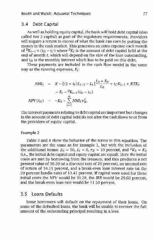
As well as holding equity capital, the bank will hold debt capital (also called tier 2 capital) as part of the regulatory requirements. Providers will require a return in excess of what the bank can earn by putting the money in the cash market. This generates an extra expense each month of DKt_l x (iD - ic) where DKt is the amount of debt capital held at the end of month t, which will depend on the size of the loan outstanding, and iD is the monthly interest which has to be paid on this debt.
These payments are included in the cash flow model in the same way as the running expenses, Et :
NMlt X - [(1 + iF )Lt-l - LtJ Lo:o Eo + icKt-l + RTKt
- Et - DKt_diD - id n
NPV(iH) = -Ko + L NM1tvfr· t=l
The interest payments relating to debt capital are important but changes in the amount of debt capital held do not alter the cash flows to or from the providers of equity capital.
Example 2
Table 3 and 4 show the behavior of the terms in this equation. The parameters are the same as for Example 1, but with the inclusion of the additional terms: Eo = 50, Et = 0, YD = 10 percent, and DKO = Ko (Le., the initial debt capital and equity capital are equal). Here the initial costs are met by borrowing from the treasury, and this produces a net present value of 36.20 (at a discount rate of 20 percent), an internal rate of return of 34.11 percent, and a break-even loan interest rate (at the 20 percent hurdle rate) of 11.41 percent. If capital were used for these initial costs the NPV would be 30.28, the IRR would be 29.60 percent, and the break-even loan rate would be 11.50 percent.
3.5 Loans Defaults
Some borrowers will default on the repayment of their loans. On some of the defaulted loans, the bank will be unable to recover the full amount of the outstanding principal resulting in a loss.

Table 3 ""-l (Xl
Cash Flows in Respect of Borrower Allowing For Expenses Month (1) (2) (3) (4) (5) (6) (7) (8)
1 5000.000 47.444 117.166 164.610 5050.000 40.269 118.338 158.607 2 4882.834 46.332 118.278 164.610 4931.662 39.326 119.461 158.787 3 4764.555 45.210 119.401 164.610 4812.201 38.373 120.595 158.968 4 4645.155 44.077 120.533 164.610 4691.606 37.412 121.739 159.150 5 4524.621 42.933 121.677 164.610 4569.868 36.441 122.894 159.335 6 4402.944 41.779 122.832 164.610 4446.974 35.461 124.060 159.521 7 4280.112 40.613 123.997 164.610 4322.914 34.472 125.237 159.709 8 4156.115 39.437 125.174 164.610 4197.676 33.473 126.426 159.898
'--9 4030.941 38.249 126.362 164.610 4071.251 32.465 127.625 160.090 0
s:: 10 3904.580 37.050 127.561 164.610 3943.625 31.447 128.836 160.283 .....
:J
11 3777.019 35.839 128.771 164.610 3814.789 30.420 130.059 160.478 III
0 12 3648.248 34.617 129.993 164.610 3684.730 29.383 131.293 160.675 ...., 13 3518.255 33.384 131.226 164.610 3553.438 28.336 132.539 160.874
» ,., .....
14 3387.029 32.139 132.472 164.610 3420.899 27.279 133.796 161.075 s:: III .....
15 3254.557 30.882 133.729 164.610 3287.103 26.212 135.066 161.278 tij.
20 2573.104 24.416 140.195 164.610 2598.835 20.723 141.597 162.320 -u ..... 25 1858.701 17.637 146.974 164.610 1877.288 14.970 148.443 163.413 III ,., ..... 30 1109.754 10.530 154.080 164.610 1120.852 8.938 155.621 164.559 ,.,
(!)
35 324.593 3.080 161.530 164.610 327.839 2.614 163.146 165.760 -<
36 163.063 1.547 163.063 164.610 164.694 1.313 164.694 166.007 0
Notes: Column (1) = Loan at start of month; Column (2) = Interest paid by borrower; Column (3) = Return O"l
of prinCipal by borrower; Column (4) = Total paid by borrower; Column (5) = Amount owed to treasury at start; Column (6) = Interest paid to treasury; Column (7) = Return of principal to treasury; and Column (8) \.0
= Total paid to treasury. \.0 (Xl

Table 4 Cash Flows to Capital Allowing For Expenses
o:J 0 0
Month (1) (2) (3) (4) (5) (6) (7) ...... ::::r
1 250.000 1.609 5.858 0.385 13.085 0.985 12.887 III ::J
2 244.142 1.571 5.914 0.376 12.932 0.970 12.545 c..
3 238.228 1.533 5.970 0.367 12.779 0.955 12.209 ::2: III
4 232.258 1.494 6.027 0.358 12.623 0.941 11.879 Vl ::::r
5 226.231 1.456 6.084 0.348 12.467 0.927 11.555 » 6 220.147 1.416 6.142 0.339 12.308 0.913 11.236 n ....
c 7 214.006 1.377 6.200 0.330 12.149 0.899 10.923 III
~
8 207.806 1.337 6.259 0.320 11.988 0.886 10.616 ~ 9 201.547 1.297 6.318 0.310 11.825 0.872 10.314 -i
In
10 195.229 1.256 6.378 0.301 11.661 0.859 10.017 n ::::r ::J
11 188.851 1.215 6.439 0.291 11.495 0.846 9.726 ii 12 182.412 1.174 6.500 0.281 11.327 0.833 9.439 c
In Vl
13 175.913 1.132 6.561 0.271 11.158 0.821 9.158 14 169.351 1.090 6.624 0.261 10.988 0.808 8.882
15 162.728 1.047 6.686 0.251 10.816 0.796 8.611 20 128.655 0.828 7.010 0.198 9.930 0.738 7.328
25 92.935 0.598 7.349 0.143 9.001 0.684 6.156
30 55.488 0.357 7.704 0.085 8.027 0.634 5.089
35 16.230 0.104 8.077 0.025 7.006 0.588 4.117
36 8.153 0.052 8.153 0.013 6.796 0.579 3.933
Sum of Present Value of Monthly Cash Flows 286.20
Less Initial Capital Allocation -250.00 Net Present Value of Loan 36.20
Notes: Column (1) = Capital at start of month; Column (2) = Interest earned on capital; Column (3) = Return '-J CD
of capital; Column (4) = Net interest on debt capital; Column (5) = Net cash flow at end of month; Column (6) = Discount factor; and Column (7) = Net present value.

80 Journal of Actuarial Practice, Vol. 6, 1998
The entire loss consists, however, of the unrecovered outstanding principal plus any previous missed interest payments plus any extra expenses incurred in the collection of the loan. Hence, it is possible for the entire loss to exceed the outstanding principal. Thus both the frequency of default and the resulting losses are crucial factors in the pricing of loans.
The notation for the cash flow model requires the following additions:
qt Probability of loan default during month t;
piq
) Probability that loan remains in effect at end of month t; t n (1 - qj);
j=1
it Expected ratio of the loss during month t to Lt.
The qt and it must be estimated in advance, perhaps from historical data relating to similar loans. The estimation of these rates, however, is a major challenge.
The expected loss during month t is qt x Pt(~i x it x Lt-I. This formulation of default recovery assumes either that the recoveries are made immediately or that (1 - it )Lt-I refers to the present value at time t of the amounts recovered at later dates.
The expected net monthly income of the loan, taking account of the defaults, becomes:
NMlt xpt(q) - [(1 + iF)pi~iLt-1 -Pt(q)LtJLo:a Eo
+ iCPt(~iKt-1 + (Pt(~iKt-1 -piq)Kt )
- Et - Pt(~i vKt_1 (iv - id + qtPt(~i (1 - idLt-l. (12)
Even with all of the features that have been incorporated in the cash flow model, the complexity of the situation is understated because loans will not be split between on-going and defaulted. There are likely to be some loans in arrears, for which provisions may be set aside before the default date (or the date of successful repayment of the amount owed). For mortgages a loan can be in arrears for more than two years before the situation is resolved, so this is not just a small matter of detail.

Booth and Walsh: Actuarial Techniques 81
Example 3
This example continues from Example 2 with the inclusion of two new parameters: qt = 0.2 percent (per month); and it = 0.2 (i.e., 80 percent of the outstanding loan is recovered). The columns in Tables 5 and 6 with asterisks have been explicitly adjusted by survival probabilities. (Some of the other columns are sums and thereby acquire the adjustment indirectly.)
The loan is only just profitable at a discount rate of 20 percent with an NPV of 1.24. The internal rate of return is 20.47 percent, and the break-even loan interest rate at the 20 percent hurdle rate is 11.98 percent. The total money received from continuing borrowers is less than the amount paid each month to the treasury, and the recovery of a substantial portion of each defaulted loan is an important component of the net monthly income.
Table 7 displays the net present values and internal rates of return using the same parameters as used to construct Tables 5 and 6, but with monthly default rates included. Table 7 demonstrates that the IRR is somewhat more variable when the initial expenses are met by borrowing rather than being met from capital.
3.6 Early Repayment of Loans
The terms of a loan sometimes will, for a fee, allow the borrower to repay the loan early. Early repayments can be an important feature of long-term loans such as mortgages where many borrowers move or may switch banks in search of the lowest interest rates. The bank cannot rely on the receipt of a full number of interest payments to provide the required profits. The problem is amplified by the fact that U.K. mortgage loans often include a reduced interest rate in the first year and by the concentration of expenses and default risks near the beginning of the loan period. The bank relies on later interest payments to make lending worthwhile.13
The loan is only just profitable at a discount rate of 20 percent with an NPV of 1.24. The internal rate of return is 20.47 percent, and the break-even loan interest rate at the 20 percent hurdle rate is 11.98 percent.
l3In the U.s.A., the problem of early repayment is dealt with mainly through the use of points, Le., interest paid in advance at start of loan for a reduced interest rate. This reduces the early repayment risk.

Table 5 00 N
Cash Flows in Respect of Borrower Allowing For Defaults Month (1) (2) (3) (4) (5) (6) (7) (8) (9)
1 0.998 5000.000 47.349 116.932 164.281 5050.000 40.269 128.201 168.471 2 0.996 4882.834 46.147 117.806 163.953 4931.662 39.247 128.827 168.074 3 0.994 4764.555 44.939 118.686 163.625 4812.201 38.220 129.458 167.678 4 0.992 4645.155 43.725 119.572 163.297 4691.606 37.188 130.095 167.282 5 0.990 4524.621 42.506 120.465 162.971 4569.868 36.150 130.737 166.887 6 0.988 4402.944 41.280 121.365 162.645 4446.974 35.108 131.384 166.492 7 0.986 4280.112 40.048 122.272 162.320 4322.914 34.060 132.037 166.097 8 0.984 4156.115 38.810 123.185 161.995 4197.676 33.007 132.695 165.702
'--9 0.982 4030.941 37.566 124.105 161.671 4071.251 31.949 133.359 165.308 0
c 10 0.980 3904.580 36.315 125.032 161.348 3943.625 30.885 134.029 164.914 ....
:::s
11 0.978 3777.019 35.059 125.966 161.025 3814.789 29.817 134.704 164.521 III
33.796 0
12 0.976 3648.248 126.907 160.703 3684.730 28.743 135.385 164.128 .....,
13 0.974 3518.255 32.526 127.855 160.381 3553.438 27.663 136.072 163.735 » n ....
14 0.972 3387.029 31.251 128.810 160.061 3420.899 26.578 136.764 163.342 c III ....
15 0.970 3254.557 29.968 129.772 159.741 3287.103 25.487 137.463 162.950 ~ 20 0.961 2573.104 23.457 134.692 158.150 2598.835 19.950 141.043 160.993 "0 .... 25 0.951 1858.701 16.776 139.799 156.574 1877.288 14.267 144.775 159.042 III
n .... 30 0.942 1109.754 9.916 145.099 155.015 1120.852 8.434 148.665 157.098 n
ro 35 0.932 324.593 2.872 150.599 153.471 327.839 2.442 152.718 155.160 -
< 36 0.930 163.063 1.440 151.724 153.164 164.694 1.224 153.549 154.773 0
Notes: Column (1) = Probability of payment at end of the month; Column (2) = Loan at start of month; Column (3) (j)
= Interest paid by borrower; Column (4) = Return of principal by borrower; Column (5) = Total paid by borrower; Column (6) = Amount owed to treasury at start; Column (7) = Interest paid to treasury; Column (8) = Return of 1.0
principal to treasury; and Column (9) = Total paid to treasury. 1.0 00
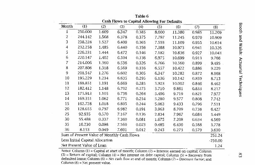
Table 6 Cash Flows to Capital Allowing For Defaults
o:l
Month (1) (2) (3) (4) (5) (6) (7) (8) 0 0
1 250.000 1.609 6.347 0.385 8.000 11.380 0.985 ....
11.209 :::J"
2 244.142 1.568 6.378 0.375 7.797 11.245 0.970 10.909 III ::::l
3 238.228 1.527 6.409 0.365 7.593 11.109 0.955 10.614 c.. :E
4 232.258 1.485 6.440 0.356 7.388 10.973 0.941 10.326 III
5 226.231 1.444 6.472 0.346 7.182 10.836 0.927 10.043 VI :::J"
6 220.147 1.402 6.504 0.336 6.975 10.699 0.913 9.766 » n 7 214.006 1.360 6.536 0.326 6.766 10.560 0.899 9.495 ....
t:
8 207.806 1.318 6.569 0.316 6.557 10.422 0.886 9.229 III
"" 9 201.547 1.276 6.602 0.305 6.347 10.282 0.872 8.968 ~
10 195.229 1.234 6.635 0.295 6.136 10.142 0.859 8.713 -i (!) n
11 188.851 1.191 6.669 0.285 5.923 10.002 0.846 8.462 :::J" ::::l
12 182.412 1.148 6.702 0.275 5.710 9.861 0.833 8.217 ..6. t:
13 175.913 1.105 6.736 0.264 5.496 9.719 0.821 7.977 (!) VI
14 169.351 1.062 6.771 0.254 5.280 9.577 0.808 7.742 15 162.728 1.018 6.805 0.244 5.063 9.433 0.796 7.511 20 128.655 0.797 6.982 0.191 3.963 8.709 0.738 6.427 25 92.935 0.570 7.167 0.136 2.834 7.967 0.684 5.449 30 55.488 0.337 7.360 0.081 1.675 7.208 0.634 4.569 35 16.230 0.098 7.560 0.023 0.485 6.430 0.588 3.778 36 8.153 0.049 7.601 0.012 0.243 6.273 0.579 3.630
Sum of Present Value of Monthly Cash Flows 251.24 Less Initial Capital Allocation -250.00 Net Present Value of Loan 1.24 Notes: Column (1) = Capital at start of month; Column (2) = Interest earned on capital; Column
C):) (3) = Return of capital; Column (4) = Net interest on debt capital; Column (5) = Recovery from w defaulted loans; Column (6) = Net cash flow at end of month; Column (7) = Discount factor; and Column (8) = Net present value.

84 Journal of Actuarial Practice, Vol. 6, 1998
Table 7 Impact of Expenses on NPV and IRR
With Eo = 50, La = 5,000, and Ko = 250 Monthly Expenses Borrowed Expenses Paid Default From Treasury From Capital Rate NPV IRR NPV IRR 0.0% 36.20 34.11% 30.28 29.60% 0.2% 1.24 20.47% -4.56 18.58% 0.4% -32.26 8.06% -37.94 8.40% 0.6% -64.37 -3.21% -69.92 -1.00%
The early termination of a loan can be put in a cash flow model in a similar manner to defaults. Let C t denote the fee charged for early repayment in month t; and Rt denote the probability that a loan that has survived to the end of month t is repaid at that time. The survival probability for a loan becomes
t piqr ) = n(1-qj)(l-Rj).
j=1 (13)
The proportion of the original loans that default at the end of month t will be qtpi~r), while the repayments will be Rt (1 - qdPi~r). The expression for net monthly income becomes:
NM1t p(qr)X(l _ q ) _ [(1 + r )p(qr) L _ p(qr) L ] La + Eo - E t -1 t F t -1 t -1 t t La t
+ icPt(~r) Kt-1 + (Pt(~r) Kt-1 - piqr ) Kt )
- (iD - ic)DKt-1pi~r) + qtPt(~r) (1 - ft)L t-1
+ Rt (1- qdPt(~r)(Lt + Cd. (14)
The approach we have taken here is an interesting contrast to the approach taken in Allan et al., (1998). That paper assumes that all loans survive the average period of seven years for a U.K. mortgage and then are repaid. Pricing is set so that the average loan provides an appropriate profit. In the U.K. this method would provide reasonable results and would provide similar results to this system where a distribution of future repayment times is used. If there were less inertia in the loan

Booth and Walsh: Actuarial Techniques 85
market, a more active fee structure may need to be developed to penalize early repayers or a probability distribution of repayment times may need to be used to estimate the expected cost and variability of cost of early repayment.
Example 4
This example builds on Tables 1 through 6 with the inclusion of early repayments. The two new parameter values are Gt = O.OILt and
SOt ~ 12 Rt = l 0.002 t > 12.
There are four extra columns in Tables 8 and 9: the probability of a loan surviving to the start of the month (i.e., pi~~\ the probability of early repayment, the amount of early repayments, and the fees accompanying these repayments.
Because there are no early repayments in the first year of this example, the first twelve months are identical to Example 3. Thereafter, NMI is initially greater than in the no repayment example, but in the last months of the loan it is less than in Example 3. NPV of 1.52 is marginally higher than without repayments, indicating that the 1 percent fee is sufficient to cover the loss of later positive cash flows. Other values for this loan include an internal rate of return of 20.58 percent and a break-even interest rate of 11.97 percent.

00 Ol
Table 8 Cash Flows in Respect of Borrower Allowing For Prepayments
Month (1) (2) (3) (4) (5) (6) (7) (8) (9) (10)
1 1.000 0.998 5000.0 47.3 ll6.9 164.3 5050.0 40.3 128.2 168.5 2 0.998 0.996 4882.8 46.1 117.8 164.0 4931.7 39.2 128.8 168.1 3 0.996 0.994 4764.6 44.9 ll8.7 163.6 4812.2 38.2 129.5 167.7 4 0.994 0.992 4645.2 43.7 ll9.6 163.3 4691.6 37.2 130.1 167.3 5 0.992 0.990 4524.6 42.5 120.5 163.0 4569.9 36.2 130.7 166.9 6 0.990 0.988 4402.9 41.3 121.4 162.6 4447.0 35.1 131.4 166.5 7 0.988 0.986 4280.1 40.0 122.3 162.3 4322.9 34.1 132.0 166.1 '-
0 8 0.986 0.984 4156.1 38.8 123.2 162.0 4197.7 33.0 132.7 165.7 c
"" 9 0.984 0.982 4030.9 37.6 124.1 161.7 4071.3 31.9 133.4 165.3
:::l $lJ
10 0.982 0.980 3904.6 36.3 125.0 161.3 3943.6 30.9 134.0 164.9 0 .."
15 0.968 0.967 3254.6 29.8 129.3 159.1 3287.1 25.4 143.0 168.4 :t> i"'
20 0.949 0.947 2573.1 23.1 132.8 155.9 2598.8 19.7 143.7 163.4 ,...,. c
25 0.930 0.929 1858.7 16.4 136.5 152.9 1877.3 13.9 144.5 158.5 $lJ
"" 30 0.912 0.910 ll09.8 9.6 140.2 149.8 ll20.9 8.2 145.4 153.6
iii·
"'0 35 0.894 0.892 324.6 2.7 144.1 146.9 327.8 2.3 146.4 148.8 "" $lJ
36 0.890 0.889 163.1 1.4 144.9 146.3 164.7 1.2 146.6 147.8 i"' ,...,. i"'
Notes: Column (1) = Probability of loan surviving to start of month; Column (2) = Probability of payment .(1)
at end of the month; Column (3) = Loan at start of month; Column (4) = Interest paid by borrower; Column < (5) = Return of principal by borrower; Column (6) = Total paid by borrower; Column (7) = Amount owed to 0
treasury at start; Column (8) = Interest paid to treasury; Column (9) = Return of principal to treasury; and en Column (10) = Total paid to treasury.
I.D I.D 00

Table 9 OJ 0
Cash Flows to Capital Allowing For Prepayments 0 ..... ::::r
Month (1) (2) (3) (4) (5) (6) (7) (8) (9) (10) (11) s:u 1 250.0 1.6 6.3 0.4 8.0 0.000
:::l 0.000 0.000 11.380 0.985 11.209 c..
2 244.1 1.6 6.4 0.4 7.8 0.000 0.000 0.000 11.245 0.970 10.909 :'E ~
3 238.2 1.5 6.4 0.4 7.6 0.000 0.000 0.000 11.109 0.955 10.614 Vl ::::r
4 232.3 1.5 6.4 0.4 7.4 0.000 0.000 0.000 10.973 0.941 10.326 .. »
5 226.2 1.4 6.5 0.3 7.2 0.000 0.000 0.000 10.836 0.927 10.043 t"I ..... 6 220.1 1.4 6.5 0.3 7.0 0.000 0.000 0.000 10.699 0.913 9.766
s::: s:u "" 7 214.0 1.4 6.5 0.3 6.8 0.000 0.000 0.000 10.560 0.899 9.495 ~
8 207.8 1.3 6.6 0.3 6.6 0.000 0.000 0.000 10.422 0.886 9.229 -i ro 9 201.5 1.3 6.6 0.3 6.3 0.000 0.000 0.000 10.282 0.872 8.968 t"I
::::r 10 195.2 1.2 6.6 0.3 6.1 0.000 0.000 0.000 10.142 0.859 8.713 :::l
ii' 15 162.7 1.0 7.1 0.2 5.0 0.002 6.033 0.060 9.697 0.796 7.721 s:::
ro 20 128.7 0.8 7.1 0.2 3.9 0.002 4.610 0.046 8.818 0.738 6.507 Vl
25 92.9 0.6 7.2 0.1 2.8 0.002 3.179 0.032 7.937 0.684 5.428 30 55.5 0.3 7.2 0.1 1.6 0.002 1.740 0.017 7.054 0.634 4.472 35 16.2 0.1 7.2 0.0 0.5 0.002 0.291 0.003 6.168 0.588 3.624 36 8.2 0.0 7.3 0.0 0.2 0.002 0.000 0.000 5.990 0.579 3.467
Sum of Present Value of Monthly Cash Flows 251.24 Less Initial Capital Allocation -250.00 Net Present Value of Loan 1.24 Notes: Column (1) = Capital at start of month; Column (2) = Interest earned on capital; Column (3) = Return of capital; Column (4) = Net interest on debt capital; Column (5) = Recovery from defaulted loans; Column (6) = Probability of early repayment; Column (7) = Early repayments; Column (8) = Early repayment fees; Column (9) = Net cash flow at end of month; Column (10) =
Discount factor; and Column (11) = Net present value. 00 'J

88 Journal of Actuarial Practice, Vol. 6, 1998
3.7 Parameter Dependence
Equation (14) is used to generate Table 10, which shows how the net present value (at a 20 percent hurdle rate), the internal rate of return, and the break-even loan rate (also at a 20 percent hurdle rate) change as the various inputs of the cash flow model are altered. These three values are given for the case where initial expenses are met by borrowing and the case where capital is used for these expenses. The standard model has the following parameters: Lo = 5,000, Ko/ Lo = 0.05, n = 36 months, n = 12 percent, rF = 10 percent, rc = 8 percent, rH = 20 percent, Eo = 50, DKo/Lo = 0.05, rD = 10 percent, Et = 0, qt = 0.2 percent, it = 0.2, Gt / Lt = 1 percent, and Rt = 0 for t ::::; 12 and = 0.2 percent for t > 12. All other entries in Table 10 differ only in one value. This standard model is the one used in Example 4.
The following observations may be drawn from Table 10:
• In all cases, NPV is greater when initial expenses are paid by borrowing rather than by using capital. (The same discount rate has been used for the two scenarios though it may be reasonable to use a lower rate when capital is used.) Clearly the option of borrowing from the treasury is cheaper than using capital to finance expenses. The borrowing option, however, would lead to greater variability of returns on a smaller amount of capital.
• In terms of the increase in break-even interest rate, the effect of the choice between these two methods of paying for the initial expenses is sensitive to the size of the loan, the hurdle rate used, and the amount of initial expenses.
• The loan rate and the cost of funds are more important than the interest rate earned on set aside capital and the interest paid on debt capital. The lending margin between the loan rate and cost of funds dwarfs all other cash flows to shareholders. Therefore the profitability is likely to be heavily dependent on the interest margin.
• The profitability is less sensitive to the hurdle rate than it is to the loan interest rate or the cost of funds. (The loan rate and the cost of fund rates are varied independently in the above table, hence the margin on the loan is changed.)

Table 10 OJ 0
The Impact of Changes in Various Inputs of the Cash Flow Model 0 .... ::J'"
Parameter Changes Borrowed Capital PJ ::::l c..
Old New NPV IRR(%) rL(%) NPV IRR(%) rL(%) ~ PJ
Standard 1.52 20.58 11.97 -4.24 18.67 12.07 til ::J'"
Lo 5,000 1,000 -35.08 -54.74 14.97 -40.85 -17.34 15.46 .. »
5,000 3000 -16.78 9.33 12.47 -22.54 9.51 12.64 t'"\ .... 5,000 10000 47.28 29.05 11.60 41.52 27.16 11.65
t: PJ
KolLo 0.05 0.01 29.42 105.25 11.50 23.66 46.54 11.60 ~.
~
0.05 0.25 18.96 36.08 11.68 13.20 27.54 11.78 --i (1)
0.05 0.10 -33.35 13.96 12.57 -39.11 13.58 12.66 t'"\ ::J'"
n 36 18 -21.66 5.89 12.66 -24.86 6.60 12.76 ::::l ..0'
36 60 26.97 27.04 11.69 18.40 23.93 11.79 t: (1)
0.12 0.11 -57.59 -0.37 11.97 -63.34 1.39 12.07 Vl rL
0.12 0.13 60.59 44.98 11.97 54.80 38.28 12.07
rF 0.10 0.08 123.75 75.92 9.92 116.78 62.01 10.04 0.10 0.11 -58.83 -0.70 13.00 -63.99 1.27 13.09
rc 0.08 0.07 -4.60 18.26 12.08 -10.37 16.78 12.18 0.08 0.09 7.60 22.93 11.87 1.84 20.58 11.97
rH 0.20 0.15 15.53 20.58 11.75 12.46 18.67 11.80 0.20 0.25 -10.94 20.58 12.19 -19.09 18.67 12.34 0.20 0.30 -22.08 20.58 12.40 -32.37 18.67 12.59
Notes: The original parameter values are given at the start of Section 3.7 and are dis-played in the column labeled "OLD" for convenience. The parameter changes are from
00 the column labeled "OLD" to the one labeled "NEW". c.o
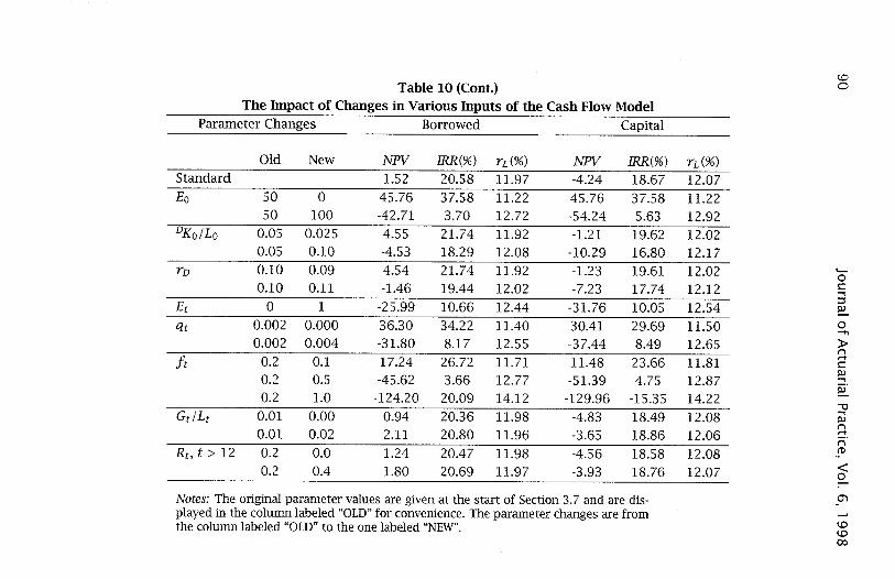
co Table 10 (Cont.) 0
The Impact of Changes in Various Inputs of the Cash Flow Model Parameter Changes Borrowed Capital
Old New NPV IRR(%) rL(%) NPV IRR(%) n(%)
Standard 1.52 20.58 11.97 -4.24 18.67 12.07
Eo 50 0 45.76 37.58 11.22 45.76 37.58 11.22 50 100 -42.71 3.70 12.72 -54.24 5.63 12.92
DKOILo 0.05 0.025 4.55 21.74 11.92 -1.21 19.62 12.02 0.05 0.10 -4.53 18.29 12.08 -10.29 16.80 12.17
rD 0.10 0.09 4.54 21.74 11.92 -1.23 19.61 12.02 ~
0 0.10 0.11 -1.46 19.44 12.02 -7.23 17.74 12.12 c ....
Et 0 1 -25.99 10.66 12.44 -31.76 10.05 12.54 ::s ~
qt 0.002 0.000 36.30 34.22 11.40 30.41 29.69 11.50 0 ...., 0.002 0.004 -31.80 8.17 12.55 -37.44 8.49 12.65 ):0-
n it 0.2 0.1 17.24 26.72 11.71 11.48 23.66 11.81
.... c s:u
0.2 0.5 -45.62 3.66 12.77 -51.39 4.75 12.87 .... iii·
0.2 1.0 -124.20 20.09 14.12 -129.96 -15.35 14.22 -\J
GtlLt 0.01 0.00 0.94 20.36 11.98 -4.83 18.49 12.08 .... s:u n
0.01 0.02 2.11 20.80 11.96 -3.65 18.86 12.06 .... n
Rt • t > 12 0.2 0.0 1.24 20.47 11.98 -4.56 18.58 12.08 _(1)
0.2 0.4 1.80 20.69 11.97 -3.93 18.76 12.07 < 0
Notes: The original parameter values are given at the start of Section 3.7 and are dis- O"l
played in the column labeled "OLD" for convenience. The parameter changes are from \D the column labeled "OLD" to the one labeled "NEW". \D 00

Booth and Walsh: Actuarial Techniques 91
• Because expenses are a higher proportion of small loans, larger loans are more profitable than small loans, both in absolute terms and per unit of capital deployed, all other things being equal. This suggests that differential interest rates with loan size and/or loan fees would be an appropriate charging policy.
• Similarly, long loans produce more profit than short loans because there is a longer time over which to amortize initial expenses.
• The amount of equity capital is more significant than the amount of debt capital because equity capital requires a higher return.
• Both initial expenses and running expenses are important.
• An extra expense of 1 per month on a loan of 5,000 requires the interest rate to be raised 0.5 percent.
• Doubling initial expenses (to 100 per loan of 5,000) would cause a greater loss than doubling the default rates (suggesting that there is a limit to the expense that should be used to assess the default risk of the borrowers).
• Though the default rate is relevant to profitability, the effect of doubling the default rate is no worse than halving the duration of the loan, starting from the parameters of the standard loan.
• Halving the loan loss fraction has a similar impact to halving the loan default rate. This is not surprising, as both parameters relate to the expected loss from a loan.
• With the parameters explored here, early repayments and associated fees are not important.
4 Variability of Default Rates and Costs
Data on mortgage arrears and possessions have been collected since 1969 by the Building Societies Association (published in the BSA Bulletin) and later the Council of Mortgage Lenders (published in Housing Finance).l4 The data suggest evidence of cyclical behavior in the 1970s in the proportions of mortgages ending in possession; see Figure 1. The
14 A mortgage is said to be in arrears whenever at least one scheduled monthly payment is not paid by a certain date. A mortgage possession (also called a repossession) occurs when the mortgage is in arrears and the bank thus terminates the mortgage and takes ownership of the house. This usually requires a court order.

92 Journal of Actuarial Practice, Vol. 6, 1998
proportions rose throughout the first half of the 1980s, peaking in the first half of 1987 with an annualized rate of 0.33 percent of mortgaged properties taken into possession. Between the first half of 1989 and the second half of 1991 the annualized rate rose from 0.17 percent of properties repossessed to 0.8 percent. Though there has been a substantial fall since then, one can still assume that future mortgage failure rates will fluctuate considerably over time.
Figure 1 Building Society Possessions and Arrears (Source: BSA & CML)
Legend 2.5 - - - -. Possessions During Year
-- Arrears 6 to 12 Months
2
0.5
o 1970 1975 1980 1985
Year
1990 1995 2000
Also, the cost to a bank of defaults on mortgage repayments varies according to the value of the property on which the mortgage is secured. This in turn depends on the change in housing prices since the mortgage was established. In the U.K. the number of mortgage failures was highest at the same time that the cost to the banks was highest, due to falling housing prices. Theoretically, the cost of default to the bank is a compound distribution formed of the probability distribution of defaults and the probability distribution of housing prices (or, more accurately, the difference between the mortgage plus arrears and the value of the house on forced sale). Suitable econometric models of either of these quantities have not been developed for the U.K.; we therefore use the empirical distribution for the cost of default from past data to estimate the sensitivity of the internal rate of return.
To examine the impact of changes in mortgage default rates and housing price inflation we calculate the internal rate of return from

Booth and Walsh: Actuarial Techniques 93
mortgage lending using historical data for default rates and house values. The loan model is the same as in Section 3 except that we ignore early repayments. The default rate (qt) and the loan loss fraction (it) are determined from data. Specifically, the loan loss fraction is set by
Ht - It it = max{O, 0.05 + It } (15)
where H t is the housing price at time t. We use a national index of housing price inflation to determine Ht / Ho. The initial housing price is related to the initial size of the loan via the loan-to-value ratio. We consider the extreme case where the initialloan-to-value ratios for mortgages that end in possession are all 100 percent. This maximizes the loss (it) and the impact of mortgage defaults on the banks' profitability. The quantity 0.05 in equation (15) represents accumulated arrears and any markdown that occurs when a possessed property is sold.
Data are available on the probability of mortgage failure in a particular year. What are needed for our calculations, however, are conditional probabilities. For example, the probability that a mortgage issued in 1985 failed in 1990, the probability that a mortgage issued in 1986 failed in 1990, and so on.
Assumptions are needed to enable us to estimate the relevant probabilities. We introduce two functions, cf> (x, y) and Q (x, y), which are defined by
cf>(x, y) = Pr[Mortgage fails during month y I Mortgage started in month x and survived to the start of month y]
qyNQ(x,y) (16)
where qy is the British national default rate (regardless of month of mortgage origin) in month y, according to British data; and N is the average length of a mortgage (taken to be 84 months); and Q (x, y) is
1 (y -x)/1200 25/1200
Q(x,y) = 673 _ (y _ x»/1200
y - x = 1,2, ... ,24 Y -x = 25,26, ... ,48 Y - x = 49, 50, ... ,72
(17)
y-x=73,74, ... .
The NPV for a loan is calculated using equation (12) but with the default probabilities (qt) replaced by cf>(x,Y) of equation (16) and the loan loss fraction given by equation (15).

94 Journal of Actuarial Practice, Vol. 6, 1998
Figure 2 shows the internal rate of return calculated by the cash flow model using data for default rates and housing price inflation. IRR is calculated for successive cohorts of loans. As we assume that no defaults happen more than six years after a loan is made, housing prices and default rates beyond 1997 will have no effect on the profitability of loans issued in 1991 or earlier. The results are calculated using a lending rate of interest n = 10.5 percent.
24.50
24.00
23.50
"if'. c '=- 23.00
~ ~ 22.50 0
f<i
'" .,. 22.00 j 21.50
21.00 1970
Figure 2 Variability of Returns Due to Changes in Default Rates and House Price Inflation
1975 1980 1985 1990 1995 Year Loan Starts
IRR is insensitive to default rates prior to 1989. Average housing prices peaked in the third quarter of 1989 and fell 12 percent over the next four years. The number of possessions peaked in the second half of 1991. Even in this severe time for the housing market the internal rate of return, based on the assumptions in our model, would have fallen only 3 percent. This illustrates the relatively low risk of mortgage lending due to loans being secured by the value of the borrowers' houses.
The model developed is flexible; for an unsecured loan the compound distribution for the cost of default will depend on default rates (which could be similar to those for mortgages) and the fraction of the loan recovered (which could be less than for mortgages). The variability of IRR probably would be much greater. Banks should take into account this risk of default both when setting interest rates that compensate
Booth and Walsh: Actuarial Techniques 95
the bank for default and when setting the hurdle rate of return, which should depend on the variability of returns. The hurdle rate should be higher for riskier (unsecured) loans.
5 The Pricing of Features
In this section the net present value will be calculated as a function of interest rate for loans with a variety of features. The purpose is to show the use of cash flow models in assessing how expensive such features are. The loans considered here are not identical to the ones used in the previous sections.
5.1 Cash Back
Many loans are provided that either give the customer some extra cash at the outset of the loan or offer some discount on the loan rate charged for the first year. These features are designed to attract customers to the bank. An alternative would be to offer a constant rate of interest throughout the loan that would be lower than the rate charged in the cash back scheme and lower than the rate charged beyond the first year in the discount scheme.
Cash back is included in the cash flow models by treating it as an extra initial expense. For example, if the money needed to provide the cash back is borrowed from the bank's treasury, it may be included in equation (14) by replacing Eo with Eo + CB where CB is the amount of cash back. If cash back is paid out of capital, it may be included in equation (11) by replacing Eo with Eo + CB.
Figure 3 shows the effect that cash back of 1 percent of the loaned amount has on the net present value. The underlying parameters of these loans are the same as used in Example 2. (There are no early repayments or defaults in these calculations). The annual interest rate required to achieve a given NPV is higher by 0.72 percent for both loan sizes; i.e., this is the cost of the cash back. This is a substantial difference in a competitive loan market.
Figure 3 also illustrates a couple of other points: (i) the importance of loan size on the interest rate required to make lending sufficiently profitable (2.9 percent extra for the smaller loan here), and (ii) the greater sensitivity of the profit to interest rates for the larger loan. The slopes of the lines are roughly proportional to the loan size.
Figure 3 is produced using the proportional repayment method for funds and assuming that the initial expenses are paid for by borrowing

96
400
300
200
100
-100
-200 10
Journal of Actuarial Practice, Vol. 6, 1998
Figure 3 Effect of Providing Cashback of 1% of Loan
Legend --_._. 5000. No Cashback
- 1000, No Cashhack •.•.•.•.•. 1000, With Cashhack
11 12 13 14 15
Annual Interest Rate on Loan (in %)
16 17 18
from the treasury. If initial expenses and cash back are both paid from capital rather than borrowing and the hurdle rate is unchanged, each NPV line in Figure 3 will shift to the right (i.e., a higher loan rate is needed to produce a given NPV). Small loans are affected more strongly than large loans because the initial expenses are proportionately larger, and likewise the loans with cash back have a larger increase in breakeven loan rate than those without cash back (again, because setting aside the capital is expensive).
Table 11 shows the parameters that interact with cash back and those that do not. It also shows how much the break-even loan rate increases if cash back of 1 percent or 5 percent is provided. The values are given for two methods of paying for initial expenses (and also cash back, as this is treated as an additional initial expense), i.e., borrowing or using capital.
These values show that the amount of cash back is important to the break-even loan rate, with the change in this rate being five times greater for the 5 percent cash back loans than for the 1 percent cash back loans. The method of financing the cash back is also important, with the capital payments requiring a larger increase in loan interest rate for a given level of cash back than if the money is borrowed from the treasury.

Booth and Walsh: Actuarial Techniques 97
·Table 11 Change in Break-Even Loan Rates, !}.YL, in Percentage Points
For Various Levels of Cash Back (CB) Parameter New Borrowing Capital Changed Value l%CB 5%CB l%CB 5%CB Standard 0.75 3.75 0.85 4.24 Lo 3,000 0.75 3.75 0.84 4.24
10,000 0.75 3.74 0.85 4.24 KolLo 2.5% 0.75 3.76 0.84 4.23
10% 0.75 3.75 0.85 4.26 n 18 1.44 7.27 1.54 7.79
60 0.47 2.35 0.57 2.84 YH 15% 0.76 3.81 0.81 4.06
25% 0.74 3.69 0.88 4.42 Eo 0 0.74 3.74 0.84 4.23
100 0.75 3.75 0.85 4.24 Et monthly 1 0.75 3.75 0.85 4.24 qt 0% 0.73 3.64 0.82 4.13
0.4% 0.77 3.86 0.87 4.36
It 0.1 0.75 3.74 0.84 4.23 0.5 0.76 3.76 0.85 4.26 1 0.76 3.78 0.85 4.28
Gt 0% 0.75 3.75 0.85 4.24 2% 0.75 3.75 0.85 4.24
Rt (t> 12) 0% 0.74 3.72 0.84 4.21 0.4% 0.75 3.77 0.85 4.26
Of the ten parameters varied in Table 11 (and for the range of values examined), seven have negligible interactions with the cost of cash back: the size of the loan, the capital backing for the loan, the initial expenses, the running expenses, the loan recovery fraction, early repayment fees, and early repayment rates (but see the comment on default rates below).
By far the most important factor in terms of the cost of cash back (other than the amount of cash back) is the length of the loan. A short loan requires the same cost to be met by fewer monthly payments; hence, a greater interest rate margin is needed. Likewise, a lower mar-gin is needed for longer loans.

98 Journal of Actuarial Practice, Vol. 6, 1 998
The two other parameters that have some (albeit minor) impact on the cost of cash back are the loan default rate and the hurdle rate of interest. The default rate's influence is due to the alteration of the average duration of the loan. (The early repayment rate is less important because the model excludes any repayments in the first year, so the impact on average duration of a change in this rate is smaller than that of the default rate.) The influence of the hurdle rate is more important for the loans where the initial expenses and cash back are paid using capital. A low hurdle rate makes the initial capital outlay on cash back less expensive in terms of the size of future positive cash flows demanded and does not require such large margins to be paid by the borrower. The cost of cash back is increased at low hurdle rates when the money for it is borrowed (this cost is decreased if capital is used).
5.2 Early Repayment and Fees
For the loans examined, early repayments are not a significant factor in terms of loan pricing. For example, using the parameters in Example 3, which has no early repayments, the break-even loan rate is 11.98 percent. If early repayments happen at the high rate of 3 percent per month for the second and third years of the loan (in which case more than half of the loans are repaid early) and no early repayment fee is charged, the break-even interest rate only rises to 12.05 percent. Early repayments are more significant if the ratio of initial expenses to the size of the loan is high and the loan is short. Nevertheless, a bank may prefer to set the interest rate appropriate to the full term of the loan and charge early repayers a fee to compensate for missed future interest payments. We find in Allan et al., (1998) that early repayments are a greater problem if higher expenses are assumed at the outset.
The fees necessary to maintain NPV in the event of early repayment of loans have been calculated for two loan sizes (1,000 and 5,000) where the interest rates charged on the loans are 15 percent and 11.6 percent, respectively, and other parameters are the same as for previous examples except that there are no defaults and no cash back. Initial expenses are financed by borrowing from the treasury. There are no repayments in the first 12 months, and the rate is constant thereafter.
Results are shown in Figure 4 where NPV is plotted against the early repayment rate (Rt). Two fans of three lines are shown; the upper is for the Lo = 5,000, rr = 11.6 percent model, the lower is for the other pair of values. In each case the lowest line of the three lines is NPV if no fee is charged for early repayment. (The proportional fund repayment scheme has been used here so that the lines slope downward as early

Booth and Walsh: Actuarial Techniques 99
repayments increase.) Let Gt denote the fee actually charged for early repayment at time t. The middle line in Figure 4 reflects a fee of 0.6 percent of the loan outstanding, Le., Gt := 0.006Lt, and the upper line reflects a fee of 2.9 percent of the loan outstanding, Le., Gt := 0.029Lt.
!l 'OJ >
j ;¥
Figure 4 Effect of Early Repayment and Fees
18
16
14
12
10
i.egcnd -NPVI --NPV2 •...•..... NPV3
-NPY4 .......... NPV5 •.....•.. NPV6
6 ~~~~~~~~~~~~~~~~~~~~ o 0.1 0.2 0.3 0.4 0.5 0.6 0.7 0.8 0.9
Early Repayment Rate (in % per Month)
For the smaller loan the repayment fee needs to be at least 2.9 percent of the outstanding loan if the bank is not to lose by allowing repayments. But for the larger loan a proportionally smaller fee (Le., about 0.6 percent) is needed. Thus, loan size is relevant to the impact of early repayment fees. The fee expressed as a percentage of the loan is inversely proportional to the loan size (although, the ratio 2.9 percent to 0.6 percent is close to the inverse of the ratio of loan sizes, Le., 1,000 to 5,000).
Figure 4 shows that there is a linear relation between early repayment rate and net present value. It is possible to find a single fee (for a given set of loan parameters) that makes the bank broadly neutral to the frequency of early repayments.
The cost of an early repayment depends on the time that it happens, with the earlier repayments being more of a problem than those that happen close to the full term of the loan. Figure 5 shows the early repayment fee necessary to keep NPV of a loan constant; this fee changes with time and is calculated using a prospective approach. The fee is equated to the present value, at the time of early repayment, of the fu-

100 Journal of Actuarial Practice, Vol. 6, 1998
ture net monthly income that would have accrued had there been no early repayment. There are also adjustments for the early return of capital less the repayment of initial expenses that had been borrowed from the treasury. The early repayment fee is given by
Figure 5 Early Repayment Fees
o ~~~~~~~~~~~~~~-L~~~~~ o 10 15 20 25 30 35
Month of Early Retirement
L t 1 ~ (. ) Gt = Ea- - Kt + - L.. NMlj(1 + iH)- ]-t
La Pt j=t+l (18)
where NMI is defined in equation (14) and does not include any adjustment for early repayments. (In the notation of equation (18), Figure 5 shows Gt / L t vs. t.)
In Figure 5 the upper line is for the La = 1, 000, YL = 15 percent combination and the lower line is for La = 5, 000 and YL = 11.6 percent. Both lines are approximately, but not exactly, linear.
If the results are calculated instead for the situation where capital is used to pay the initial expenses (so the EaLt / La term is not needed in the above equation) and a higher interest rate is charged because this method is more expensive, the outcome is almost identical. This indicates that the costs of early repayment are not significantly dependent on the method used to pay for the initial expenses.

Booth and Walsh: Actuarial Techniques 101
We conclude that there are three approaches one can take to model early repayments and assess the risk. Each of the three approaches can be used with the 25 year (full-term) loan model used here or with the seven year (average term) loan model used in Allan et al., (1998).
The first approach takes a best estimate of repayment rates and price to determine the correct average price charged to all borrowers. The problem with this approach is that it is deterministic and the risk of changed early repayment rates only can be assessed by deterministic scenario testing.
The second approach uses an actuarially neutral charging structure so that repayment fees can be charged for early repayments at any time. The fee would leave the internal rate of return of the loan unchanged whatever the time of surrender. Such an approach, which the authors believe will develop further in the U.K., would pass repayment risk to the borrower. It, therefore, would not require a stochastic approach.
The third approach involves a stochastic model of repayments to assess the variability of the internal rate of return given a reasonable model of early repayments. Repayments depend on the repayment fee and the degree of competition in the mortgage market. We believe that such an approach is unnecessary in the U.K. but may be necessary where the market is resistant to actuarially neutral early repayment fees. This is an area we leave for further research.
Our model has assumed a fixed interest rate throughout the term of the loan. In the U.K. most mortgages are variable rate. The results of the model would not be Significantly altered if a variable rate were to be used as long as the interest margin (the difference between the loan rate paid by the borrower and the cost of funds for the bank) remained constant. It is the margin rather than the absolute level of interest rates that is important.
A more significant problem would arise when using the model to price fixed rate loans. It would be necessary to deal with the problem of borrowers exercising an option to repay early if variable interest rates fall. An option pricing approach to valuing that option could be used. Otherwise, three approaches are possible. First, the bank could investigate, using deterministic scenario testing, the effect of yield curve changes on profitability. The bank must make appropriate provisions for the exercise of an option to repay early. A second approach is to charge the borrower a penalty for early repayment. This is common in the U.K. The penalties are suffiCiently high (for example, six months' interest for early repayment of a five year loan) to provide a significant disincentive for early repayment. Prepayment need not be a problem with the correct charging structure. Third, if the market will not bear
102 Journal of Actuarial Practice, Vol. 6, 1998
prepayment penalties (or regulation prevents them), a fully stochastic model may be appropriate to enable the bank to assess the risk of prepayments caused by yield curve movements as well as other causes.
5.3 Risk Decreasing With Time
In this example the expected default rate and cost of default decrease with the time since the inception of the loan. The effect of varying the interest rate during the course of the loan to reflect this risk is examined.
For mortgages the risk to the bank is concentrated in the first few years of the loan. If a borrower has repayment problems later, the mortgage will be covered by the house value unless housing prices have fallen in nominal terms by more than the amount of the loan repaid. The bank could rearrange the mortgage or take possession of the property.
If risk decreases with time, shouldn't the interest rate? In practice the opposite is often the case as banks try to attract borrowers by providing low introductory rates.
The following example examines the possible benefit of varying the interest rate as the loan progresses. Several parameters are unchanged from previous examples: rH = 20 percent, rF = 10 percent, rc = 8 percent, rT2 = 10 percent, and Et = O. Those parameters that differ from previous examples are Lo = 100,000, Eo = 500, KolLo = T2Ko/Lo = 2.5 percent, and n = 25 years. Also, default and repayment rates are different, and various values are considered for the loan interest rate. The defaults have the following pattern. The loan loss fraction is given by
j; = { 0.05 + (Lt - L36) /L36 t =s; 36 tOt> 36.
There are no losses after three years as the house value should be enough to cover the mortgage. Before three years the loss fraction decreases with time as part of the loan is repaid, but it is always at least 5 percent of the outstanding loan value. Otherwise, some form of rearrangement may be a more likely outcome than a default. In the first three years the default rate is either 0.2 percent per month or 0.4 percent per month. (Results are given for both values.)
Mortgage loans often end early as persons move before the repayment is complete or transfer to another bank before the full term is finished. The repayment pattern used is

Booth and Walsh: Actuarial Techniques 103
{ 0 t ~ 36
Rt = 0.015 t > 36.
It is not necessary that the early repayments start at the same time as the defaults stop, but a duration of one to five years is likely to be appropriate for both values. No fee is charged for early terminations of the mortgage in the model considered here. With this repayment pattern, roughly half of mortgages have ended by the seventh year.
How should interest rates be changed to take into account declining default risk? The equation for net monthly income for a set of loans (see, for example, equation (14)) includes
NMI = [i[ - (iL + f)q]L + Terms not involving defaults or i[.
This suggests that if iL - (iL + f)q is kept constant as q and f change, the profitability of a loan will be broadly neutral to default risk. Let q and (qf) be defined as:
Then the invariant requirement leads to an interest rate set by
(1 - q}ifean + (qf - (qf) 1-q
When the default rate in the first three years is 0.2 percent per month the weighted averages q and (qf) are 0.0727 percent and 0.0048 percent, respectively. When the default rate is 0.4 percent these two values are 0.1489 percent and 0.0098 percent, respectively.
The following results are obtained using a simpler formula for the risk interest rate, viz.:
.Risk . q x f - (qf) tL = tL + 1 -q
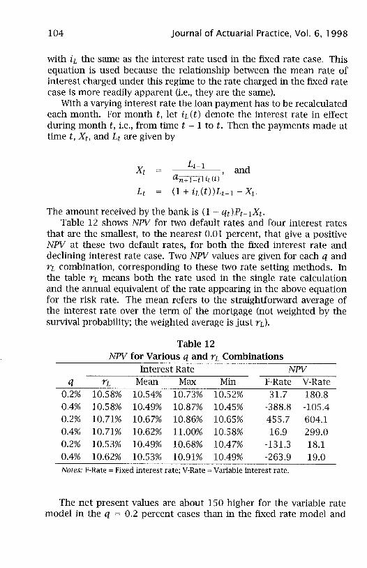
104 Journal of Actuarial Practice, Vol. 6, 1998
with ir the same as the interest rate used in the fixed rate case. This equation is used because the relationship between the mean rate of interest charged under this regime to the rate charged in the fixed rate case is more readily apparent (i.e., they are the same).
With a varying interest rate the loan payment has to be recalculated each month. For month t, let ir (t) denote the interest rate in effect during month t, i.e., from time t - 1 to t. Then the payments made at time t, Xt, and Lt are given by
Lt-1 and an +1- t I idt)
(1 + idt»Lt-1 - Xt·
The amount received by the bank is (1 - qdPt-1Xt. Table 12 shows NPV for two default rates and four interest rates
that are the smallest, to the nearest 0.01 percent, that give a positive NPV at these two default rates, for both the fixed interest rate and declining interest rate case. Two NPV values are given for each q and rL combination, corresponding to these two rate setting methods. In the table n means both the rate used in the single rate calculation and the annual equivalent of the rate appearing in the above equation for the risk rate. The mean refers to the straightforward average of the interest rate over the term of the mortgage (not weighted by the survival probability; the weighted average is just n).
Table 12 NPV for Various q and n Combinations
Interest Rate NPV q n Mean Max Min F-Rate V-Rate
0.2% 10.58% 10.54% 10.73% 10.52% 31.7 180.8 0.4% 10.58% 10.49% 10.87% 10.45% -388.8 -105.4 0.2% 10.71% 10.67% 10.86% 10.65% 455.7 604.1 0.4% 10.71% 10.62% 11.00% 10.58% 16.9 299.0 0.2% 10.53% 10.49% 10.68% 10.47% -131.3 18.1 0.4% 10.62% 10.53% 10.91% 10.49% -263.9 19.0 Notes: F-Rate = Fixed interest rate; V-Rate = Variable interest rate.
The net present values are about 150 higher for the variable rate model in the q = 0.2 percent cases than in the fixed rate model and

Booth and Walsh: Actuarial Techniques 105
280 higher for the q = 0.4 percent cases (for comparison, the initial capital outlay is 2500). Alternatively, instead of making a larger profit at the same (weighted average) interest rate, a lower average rate can be charged, as shown in the last two lines.
Moreover, the importance of the default rate is reduced when this flexible interest rate is used. For example if the rate had been set at 10.58 percent in anticipation of the lower default rate, the reduction in NPV that happens if the default rate proves to be 0.4 percent per month is 420 if the fixed rate is used and 286 if the flexible rate is used. This method only works if the risk adjustments to the interest rates are based on the 0.4 percent value. If they are not, the loss is just as great as in the fixed rate case.
This example illustrates that average interest rates can be reduced if risk-related pricing is introduced. The suggested differences in the average rates charged are not large, with reduction in the rates less than 0.1 percent.
6 Summary and Conclusions
Cash flow models that are used in other areas of actuarial work could be used in banking to price loans. Often bank lending is priced by looking at the whole book of business together and ensuring that the margin is adequate to provide the required return on capital on the business as a whole. Adjustments to the margin will generally be made to allow for the risk profiles of different borrowers. A cash flow approach would consider explicitly the cash flows that were expected for a particular category of loans. It would therefore be possible to set an interest margin, appropriate to that category that allowed explicitly for: the capital used to back a particular category of loans; the expenses of a particular category of loans; and the risk of a particular category of loans. The cash flow approach can also handle the many interest rates that are relevant to bank lending. The following interest rates give rise to cash flows: interest charged on the loan; interest paid by the lender to the source of the money lent; hurdle rate of return on equity capital; rate of interest to be paid on debt capital; interest earned on set-aside equity capital.
Having determined the cash flows pertaining to a particular category of loan, the cash flow model can be used to make business decisions such as determining the interest margin to be charged or determining whether the interest margin available on a category of lending in the market makes the loan sufficiently profitable. For marketing reasons,

106 Journal of Actuarial Practice, Vol. 6, 1998
it may be appropriate to give cross subsidies between categories of lonns. The cash flow model allows the effect of these cross subsidies to be quantified.
When lending is secured (for example mortgage lending) the effect of defaults is not significant but in general defaults are important. The model has been extended to deal with defaults but more empirical work is necessary to find reasonable models of default rates and the loss incurred by a bank on defaults. Various ways of dealing with prepayments are discussed. Prepayments can cause difficulty for two reasons: first initial expenses may not be recouped if a loan is prepaid; second, if a loan is given at a fixed rate of interest there is a financial interest rate option against the lender. In the U.K. market, it may be possible to develop charging structures so that early repayments do not have a material financial effect on the bank (prepayment penalties are common). Where this is not possible, stochastic modeling of prepayments should be performed.
The model is extended to include pricing for loan products which involve cash backs and prepayment fees. The sensitivity of the model to various parameters is tested and it is found that expenses; the interest margin; the size of loan; and the duration of the loan are the most important parameters. Banks may wish to differentially price loans to a greater extent than is currently the case to allow for size and duration of a loan. Alternatively, as has been mentioned above, prepayment fees or other charging structures could be used to ensure that loans which are prepaid are still profitable.
The main areas for further work are the development of better models for estimating the costs of default and the modeling of prepayments where charging structures do not make the bank indifferent to prepayments.
References
Allan, J.N., Booth, P.M., Verrall, R.J.. and Walsh, D.E.P. "The Management of Risks in Banking." Presented on February 23, 1998 to the Institute of Actuaries. Forthcoming in Institute of Actuaries Session Meeting Paper, (1998).
Altman, E.I. Corporate Financial Distress. New York, N.Y.: John Wiley & Sons, 1983.

Booth and Walsh: Actuarial Techniques 107
Altman, E.!. "Corporate Bond and Commercial Loan Portfolio Analysis." Wharton School Working Paper Series, pp. 96-41. Philadelphia, Pa.: University of Pennsylvania, 1996.
Brealey, RA, and Myers, S.c. Principles of Corporate Finance. New York, N.Y.: McGraw Hill, 1991.
British Bankers' Association. Annual Abstract of Banking Statistics. Banking Act Report. London, England: Bank of England, 1995.
Building Societies Association. "Trends in Mortgage Arrears." BSA Bulletin 43 (1985): 18.
Davis, E.P. "Bank Credit Risk." Bank of England Working Paper Series 8 (1993).
Griffin, K. "The Retail Banking Industry in Australia." Institute of Actuaries of Australia session meeting paper (1996).
Hare, D.].P., and McCutcheon, ].]. An Introduction to Profit Testing. Lon-don, England: Institute of Actuaries, 1991.
Higson, c.]. Business Finance. London, England: Butterworths, 1986.
Council of Mortgage Lenders. "Table 25" Housing Finance 32 (1996): 46.
Hylands, ].F., and Gray, L.]. Product Pricing in Life Assurance. London, England: Institute of Actuaries, 1989.
Lewin, G.c., Carne, SA, DeRivaz, N.F.C., Hall, R.E.G., McKelvey, K.J.. and Wilkie, M.A. "Capital Projects." British Actuarial Journal, 1 part 2 (1995): 155-249.
Squires, R.]. Unit Linked Business. London, United Kingdom: Institute and Faculty of Actuaries, 1986.
Taffier, R.J. "Forecasting Company Failures in the UK Using Discriminant Analysis and Financial Ratio Data." Journal of the Royal Statistical Society, Series A, 145 part 3 (1982): 342-358.
Appendix A: How Credit Risk is Assessed
Corporate Loans
A bank can group large borrowers according to expected default risk. The allocation of a borrower to a risk group generally is based on accounting ratios. Statistical techniques (regression or multiple discriminant analysis) are applied to historical data on bankruptcies or loan defaults with these accounting ratios to produce a set of weights for the ratios. Any potential borrower's accounts can be studied to provide a score that is intended to be a predictor of default risk.

108 Journal of Actuarial Practice, Vol. 6, 1998
The procedure has been in widespread use since the 1960s, and some of the formulae used have been published. It is often found, however, that weighting factors determined from one data set are not the same as those from another set: e.g., U.S.-derived weights are not applicable in the U.K., and 1970s values are not useful now.
A review of many analyses of corporate default is presented in Altman (1983). For a paper relating to risk factors in the U.K., see Taffler (1982). References to more recent papers are found in Altman (1996). Altman (1996) also provides a formula for a score that is a predictor of default risk, with a higher score indicating a lower probability of default:
where
Xl Working capital/total assets; X2 Retained earnings/total assets; X3 Earnings before interest and taxes/total assets; and X4 Equity (book value)/totalliabilities.
Also, Cl, C2, C3, and C4 are positive constants.
Personal Loans: Credit Scoring
The method of assessing the risks in personal loans is called credit scoring. The statistical techniques used are similar to those used for large corporate loans (e.g., discriminant analysis), but the factors in the model change (there are no audited accounts to use).
There is considerable danger in using past data to predict future bad debts. The economic background is likely to influence the overall level of bad debts. Within this overall trend, the credit score should indicate some ranking of risk.
For a given type of loan, the most important data are provided by credit agencies. Evidence of existing bad debts with other banks and evidence of successful maintenance of credit repayments are relevant. Other demographic data as provided on loan application forms may be used, but are not always major influences. (One reason is that banks find that short application forms are useful in attracting customers.) A third source of information is behavior, Le., the credit history of a

Booth and Walsh: Actuarial Techniques 109
loan applicant who is an existing customer of the organization. All of the factors can be combined onto a scorecard, and historical data will provide default rates and costs of default versus score.
The construction of a scorecard usually is done by a specialist agency. Typically a new scorecard will be prepared every two or three years. Around 1,000 to 2,000 bad loans are needed (and an equal number of good loans) to provide statistically sound weights. Given that a default rate of only a few percent a year is not uncommon, this number of bad loans requires a large portfolio, a long base period, or a weak definition of bad. In practice the last option is likely to be selected.
It is appropriate to have different scorecards for different products (e.g., mortgages and credit cards) and for different categories of customer (e.g., new or existing customer).
There is an important limitation on the reliability of default rate predictions; the data are for a select set of the population, Le., persons accepted for loans a few years ago. Risk factors that are unimportant among this group may be Significant in the population of future loan applicants.
Once a score has been calculated for a loan applicant, the most common approach in bank lending is a straight accept or reject decision (e.g., accept the application if the score is greater than, say, 100). This contrasts with risk-based pricing in insurance where premium rates vary with risk rather than being one rate for all accepted. The equivalent response in terms of lending would be to charge a rate of interest that varies with risk. This method has been introduced in some areas of bank lending. An alternative method, used in practice with credit cards, is for a bank to operate several cards (perhaps under different names) with different interest rates. To be accepted for a low interest rate card, a higher score will be needed than for the higher interest rate cards.
Appendix B: Uniform Repayments to the Treasury
This section expands possible ways in which the bank could repay money to the bank's treasury.
The paper has been based on the assumption that the bank always owes to the treasury an amount equal to the amount that the borrower owes. (Initial expenses are also paid in the same pattern.) An alternative is that the initial amount borrowed from the treasury (for loans and initial expenses) are amortized over the period of the loans and paid

110 Journal of Actuarial Practice, Vol. 6, 1998
in equal installments irrespective of whether some loans default or are repaid early.
If there is a difference between the amounts owed by the bank (to the treasury) and to the bank (by the borrower) this does not mean that there is idle cash available. The bank holds no money other than capital (which is invested in the wholesale cash market); all of the money it receives is immediately paid to the treasury or assigned to the providers of capital as profit.
Under the uniform repayment scheme the equation for net monthly income, which is comparable to the equation (14), is:
NMl t xpiqr ) (1 - qd _ Lo + Eo alil iF
+ icpi~~) Kt-l + (Pt(~~) Kt-l - piqr) Kt ) - Pt(~~)DKt_l (iD - ic)
- Et + qtPt(~~) (1 - fdLt-l + Rd1 - qt)Pt(~~) (L t + Gd.
(Everything is the same except for payments to the treasury.) Figure B1 illustrates the Significance of the two fund repayment pat
terns. The parameters used in producing this figure are the same as for the second spreadsheet example, except that early repayments are included (but there are no early repayments allowed in the first year). A loan interest rate of rr = 11.45 percent is chosen to make NPV close to zero. (At the maximum early closure rate shown, 0.2 percent, 95 percent of loans last the duration.)
Figure B1 shows that even without premature repayments there is a difference in the value of this loan under the two methods of funding. The proportional method gives a higher value because there is a slight delay in the timing of repayments to the treasury. (These repayments are irlitially less than in the uniform case, but are greater later. In total they are a little larger under the proportional method.)
Also, early repayments reduce the value of the loan, as far as the bank is concerned, when the proportional method of fund repayment is used. Early repayments are welcome under the uniform scheme, however. Although it may seem unreasonable for a bank to want a profitable loan to stop, the improvement shown in the figure is not wrong. The result depends on the bank being able to secure funds from the treasury at a rate of interest below the hurdle rate that can be retained after some of the loans have been repaid (or defaulted).
The figure illustrates the point that the way the funding is arranged or the method of bookkeeping selected can be more important in de-

Booth and Walsh: Actuarial Techniques
3.00
2.50
2.00
1.50
1.00
0.50
0.00
-0.50
-1.00
Figure Bl Different Repayment Patterns for Funds
0.00 0.02 0.04 0.06 0.08 0.10 0.12 0.14 0.16 0.18 0.20 Early Repayments per Month (in %)
111
termining the profitability of a class of loans than a key feature of the loan (in this case the early repayment pattern)_
The steepness of the line for the uniform repayment case shows that the profitability of the loan is likely to be more volatile if this scheme is used. Also, the internal rate of return of loans financed by the uniform repayment scheme is more sensitive to the default rates, when the default rates are high than they would be under the proportional repayment scheme. In this sense there is more risk accepted by the providers of capital when a uniform repayment plan is used, and a higher return therefore may be required.

112 Journal of Actuarial Practice, Vol. 6, 1998