Risk Control of Mean-Reversion Time in Statistical Arbitragecdar.berkeley.edu/wp-content/uploads/2018/01/statarbslideUCB.pdf · 4.Trading: optimal allocation and PnL 5.Results with

Risk Control of Mean-Reversion Time in StatisticalArbitrage

George PapanicolaouStanford University

CDAR Seminar, UC Berkeley

April 26, 2018

with Joongyeub Yeo”Risk Control of Mean-Reversion Time in Statistical Arbitrage”,J. Yeo and G. Papanicolaou, Risk and Decision Analysis, vol 6, 2017,p. 263-290.

G. Papanicolaou, CDAR-UCB Risk Control 1/24

Outline:

Statistical Arbitrage: It is a widely practiced general form of pairs trading

1. The Merton problem and pairs trading

2. Factor model for US equity returns and its implementation

3. Controlling the mean reversion of residuals

4. Trading: optimal allocation and PnL

5. Results with daily S&P500 data (2004-2014) exactly as they wouldbe obtained in real time

6. Academic studies of statistical arbitrage: Andrew Lo1 (MIT), andMarco Avellaneda2 (NYU-Courant)

1Hedge Funds: An Analytic Perspective, Princeton University Press, 20102Statistical arbitrage in the US equities market, Quantitative Finance, 2010


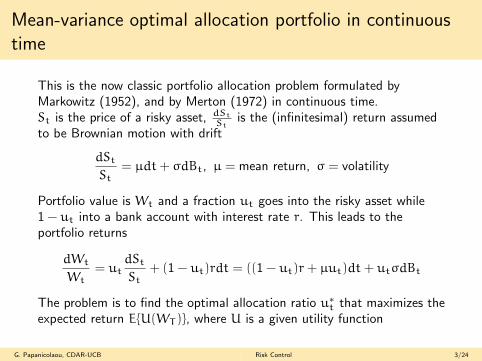
Mean-variance optimal allocation portfolio in continuoustime

This is the now classic portfolio allocation problem formulated byMarkowitz (1952), and by Merton (1972) in continuous time.St is the price of a risky asset, dSt

Stis the (infinitesimal) return assumed

to be Brownian motion with drift

dSt

St= µdt+ σdBt, µ = mean return, σ = volatility

Portfolio value is Wt and a fraction ut goes into the risky asset while1 − ut into a bank account with interest rate r. This leads to theportfolio returns

dWt

Wt= ut

dSt

St+ (1 − ut)rdt = ((1 − ut)r+ µut)dt+ utσdBt

The problem is to find the optimal allocation ratio u∗t that maximizes the

expected return E{U(WT )}, where U is a given utility function


Merton portfolio, log utility, zero mean return

Optimal allocation ratio u∗ is a constant (fundamental portfoliotheorem) and wealth log growth rate are

u∗ =µ− r

σ2, r+

(µ− r)2

2σ2(= r+ Sharpe ratio squared/2)

Since d log St = (µ− σ2/2)dt+ σdBt, when µ = σ2

2 mean log return ofstock is zero. Then

u∗ =1

2(1 −

2r

σ2)

and portfolio log growth rate is

r+σ2

8(1 −

2r

σ2)2

If 2rσ2 is small and σ > .5, say, then the constant portfolio allocation

strategy will realize considerable growth above the basic interest rateeven when the stock or index is not growing at all. The portfolioallocation ratio in stock will never be more than 50%. The bestenvironment for this kind of portfolio strategy is: low real interest ratesand highly fluctuating stocks that have no (log) growth.


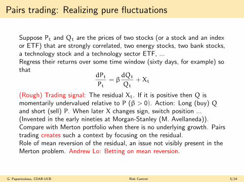
Pairs trading: Realizing pure fluctuations

Suppose Pt and Qt are the prices of two stocks (or a stock and an indexor ETF) that are strongly correlated, two energy stocks, two bank stocks,a technology stock and a technology sector ETF, ...Regress their returns over some time window (sixty days, for example) sothat

dPt

Pt= β

dQt

Qt+ Xt

(Rough) Trading signal: The residual Xt. If it is positive then Q ismomentarily undervalued relative to P (β > 0). Action: Long (buy) Qand short (sell) P. When later X changes sign, switch position ...(Invented in the early nineties at Morgan-Stanley (M. Avellaneda)).Compare with Merton portfolio when there is no underlying growth. Pairstrading creates such a context by focusing on the residual.Role of mean reversion of the residual, an issue not visibly present in theMerton problem. Andrew Lo: Betting on mean reversion.


Generalized ”pairs” trading: Factor decomposition

We start with the N× T matrix of stock returns, R and decompose itinto factors:

R = LF+U (1)

where F is a p× T matrix of factors L is an N× p matrix of factorloadings, U is a N× T matrix of residuals.Only R is observable, so L, F, and U must be estimated. We obtainfactors using principal components analysis (PCA) so only their numberp is to be determined. Next, the factor loadings (L) are estimated bymultivariate regressions of R on the subspace spanned by F. Finally, theresidual (U) is expressed as the remaining parts, after subtracting theestimated common factors from the original returns:

U = R− LF. (2)

where the hat ( · ) notation indicates estimators, since only R isobservable.All this in a time window that is rolling forward in time.


What do we know about the factors?

• In Economics: The three-factor models for stock returns of Frenchand Fama (1992).

• In Econophysics: How to extract factors using PCA so that theresiduals have a correlation matrix that has Marchnko-Pastur (purelyrandom) statistics. Many papers in late nineties. Survey ofBouchaud and Potters (2009) presents the ideas and methods inperspective.

• Some startling empirical facts: The principal (left) singular vector ofthe return matrix R when ordered by size lines up with the marketcapitalization of the stocks.

• The correlations of returns ”uncover” market capitalization andmarket sectors without knowing anything other than the (time seriesof the) returns themselves.


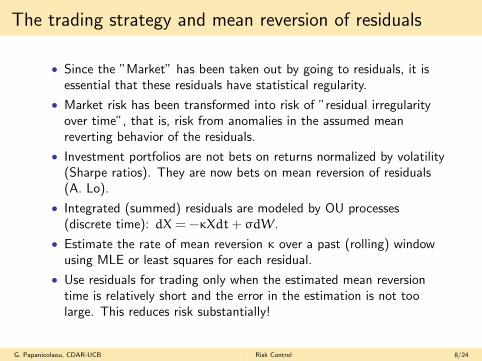
The trading strategy and mean reversion of residuals

• Since the ”Market” has been taken out by going to residuals, it isessential that these residuals have statistical regularity.

• Market risk has been transformed into risk of ”residual irregularityover time”, that is, risk from anomalies in the assumed meanreverting behavior of the residuals.

• Investment portfolios are not bets on returns normalized by volatility(Sharpe ratios). They are now bets on mean reversion of residuals(A. Lo).

• Integrated (summed) residuals are modeled by OU processes(discrete time): dX = −κXdt+ σdW.

• Estimate the rate of mean reversion κ over a past (rolling) windowusing MLE or least squares for each residual.

• Use residuals for trading only when the estimated mean reversiontime is relatively short and the error in the estimation is not toolarge. This reduces risk substantially!


The long/short trading strategy with normalized residualsas signals: Buy low - sell high

When the trading signal hits 1.25, it is presumed to be over-valued, so wesell the stock to open the short position (green dots), expecting it to godown soon. If it hits 0.5, we buy the stock to close the short position,which leads us to obtain profits. Similar strategy can be applied to theopen/close of long position (red dots).


The trading algorithm: Yes, buy low and sell high. Butwith what allocation?

The dollar amount qi, i = 1, 2, . . . ,N (signed for long/short) to invest isdetermined at each time t by the following:

Market-neutrality :∑i

Likqi = 0, for each k=1,. . . ,p (3)

Dollar-neutrality :∑i

qi = 0 (4)

Total Leverage :∑i

‖qi‖ = I (5)

Long/Short : sgn(qi) is given by trading signals. (6)

Here L is the factor loading matrix, p is the number of factors, and I isthe total leverage level.


Profit and Loss

The performance from trading can be measured by the cumulativeprofit-and-loss (PnL):

Et+∆t = Et + Etr∆t+

N∑i=1

qitRit∆t−

N∑i=1

qitr∆t−

N∑i=1

|qi(t+∆t) − qit|ε (7)

Et is the value of the portfolio at time t,r is the reference interest rate,ε is for frictional cost (measured in basis points).Note that the fourth term on the right hand side must be zero if thedollar neutral condition is completely satisfied. However, there isnumerical tolerance imposed for the feasibility, so we keep that term here.


The US equities data used in backtesting

• SP500 daily data from 2005 to 2014, split into 5 time periods:2005-2007 (before crisis), 2007-2008 (in crisis), 2009-2010 (crisisrecovery), 2011-2012 (post crisis I), 2013-2014 (post crisis II).

• Use only 378 stocks from the SP500 to have uninterrupted recordsand avoid necessary preprocessing of data.

• Use 30-120 day rolling windows in the analysis

• Use 1-20 PCA factors in generating residulas

Avellaneda (2010 and later) uses a much larger set of equities, beyondthe SP500 (the over one billion capitalization group). He also uses ETFsfor factors, both real and synthetic ones.


Risk control with estimated mean reversion time ofresiduals

• Since risk has migrated into the mean reverting behavior of theresiduals, we need to control it through the estimates of meanreversion times.

• The error (in MLE) is proportional to the reciprocal square root ofthe time window. And we cannot use large time windows becauseinformation in the residuals becomes ”stale” (non-stationary).

• Typical tradeoff in applied science (channel estimation, geosciences,biology, genomics, etc): We want to use a large enough datawindow to have statistical stability but also one that is small enoughto have approximately stationary statistical properties.

• Bottom line: Use residuals that have (a) relatively short meanreversion times and (b) relatively high statistical confidence score:Use diversity by proper selection in a high-dimensional setting.


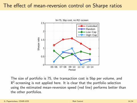
The effect of mean-reversion control on Sharpe ratios

05−06 07−08 09−10 11−12 13−140

0.5

1

1.5

2

2.5

Period

Sha

rpe

ratio

N=75, 5bp cost, no R2−screen

ControlledRandomLow−CapHigh−Cap

The size of portfolio is 75, the transaction cost is 5bp per volume, andR2-screening is not applied here. It is clear that the portfolio selectionusing the estimated mean-reversion speed (red line) performs better thanthe other portfolios.


Sample results of cumulative PnL for each period;Controlled

2005 2006 2007 2008 2009 2010 2011 2012 2013 20140.9

1

1.1

1.2

1.3

1.4

Time (year)

Cum

ulat

ive

PnL

Controlled Portfolio. Cost=5bp

2005−2006 (SR: 2.96)2007−2008 (SR: 2.57)2009−2010 (SR: 2.24)2011−2012 (SR: 2.59)2013−2014 (SR: 1.73)

2005 2006 2007 2008 2009 2010 2011 2012 2013 20140.9

1

1.1

1.2

1.3

1.4

Time (year)

Cum

ulat

ive

PnL

Controlled Portfolio. Cost=10bp

2005−2006 (SR: 1.09)2007−2008 (SR: 1.40)2009−2010 (SR: 0.90)2011−2012 (SR: 0.59)2013−2014 (SR: 0.35)

Two transaction costs (of 5bp and 10bp). Portfolio size is N = 75;Number of factors is 5; Window length is 30 days. R2-screening isapplied.


The out-of-sample performance from four differentportfolios

05−06 07−08 09−10 11−12 13−140

0.5

1

1.5

2

2.5

Period

Sha

rpe

ratio

N=75, 5bp cost, no R2−screen


05−06 07−08 09−10 11−12 13−140

0.5

1

1.5

2

2.5

PeriodS

harp

e ra

tio

N=75, 5bp cost, R2−screen


Number of selected stocks is 75; Transaction costs are 5bp; Left:Without R2-screening. Right: With R2-screening. The overall level ofperformance is enhanced by selective trading based on R2-screening.


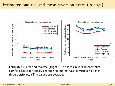
Estimated and realized mean-reversion times (in days)

05−06 07−08 09−10 11−12 13−14

7

8

9

10

11

12

13

Period

Estimated mean−reversion time

Est

imat

ed m

ean−

reve

rsio

n tim

e (d

ays)


05−06 07−08 09−10 11−12 13−14

7

8

9

10

11

12

13

Period

Realized mean−reversion time

Rea

lized

mea

n−re

vers

ion

time

(day

s)


Estimated (Left) and realized (Right). The mean-reversion controlledportfolio has significantly shorter trading intervals compared to otherthree portfolios. (The values are averaged).


The performance surface as a function of number offactors (p) and window length (T)

0

5

10

15

20

40

60

80

100

120−4

−2

0

2

Window length

Low transaction cost (ε=5bp)

Number of factors

Sha

rpe

ratio

0

5

10

15

20

40

60

80

100

120−4

−2

0

2

Window length

High transaction cost (ε=15bp)

Number of factors

Sha

rpe

ratio

The performance surface as a function of number of factors (p) andwindow length (T), for two different transaction costs.


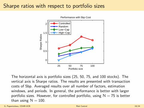
Sharpe ratios with respect to portfolio sizes

25 50 75 100

0

0.5

1

1.5

2

Portfolio size

Sha

rpe

Rat

ios

Performance with 5bp Cost


The horizontal axis is portfolio sizes (25, 50, 75, and 100 stocks). Thevertical axis is Sharpe ratios. The results are presented with transactioncosts of 5bp. Averaged results over all number of factors, estimationwindows, and periods. In general, the performance is better with largerportfolio sizes. However, for controlled portfolio, using N = 75 is betterthan using N = 100.


Performance with and without optimization for assetallocation

05−06 07−08 09−10 11−12 13−140

0.5

1

1.5

2

2.5

Period

Sha

rpe

ratio

Effect of Optimization for Allocations

With optimizationWithout optimization

Without optimized asset allocations, the trading strategy is unstable andis not market-neutral.


Dynamics of number of factors that explain different levelsof variance

2005 2006 2007 2008 2009 2010 2011 2012 2013 20140

5

10

15

20

25

30Window: 60 days

Num

ber

of fa

ctor

s

Year

20%30%40%50%60%SP500

2005 2006 2007 2008 2009 2010 2011 2012 2013 20140

5

10

15

20

25

30Window: 120 days

Num

ber

of fa

ctor

s

Year

Window: 60 days (top) and 120 days (bottom). N = 378 stocks.


The largest eigenvalue of correlation matrix of normalizedoriginal returns with moving window

2005 2006 2007 2008 2009 2010 2011 2012 2013 20140

0.2

0.4

0.6

0.8

1Dynamics of largest eigenvalue

Leve

l of v

aria

nce

expl

aine

d by

by

the

larg

est e

igen

valu

e

Year

Window: 60 daysWindow 120 days

The shorter windows response is more sensitively to the market.


Statistics of mean reversion time and R2 values (20 factors)

0 20 40 60 80 100 120 140 1600

1

2

3

4

5

6

7

8x 10

4 Distribution of mean−reversion time (window=60 days)

estimated mean−reversion time (days)

freq

0 20 40 60 80 100 120 140 1600

1

2

3

4

5

6

7

8x 10

4 Distribution of mean−reversion time (window=120 days)


freq

0.4 0.5 0.6 0.7 0.8 0.9 10

1

2

3

4

5

6

7

8

9x 10

4 Distribution of R2 value (window=60 days)

R2 value

freq

0.4 0.5 0.6 0.7 0.8 0.9 10

1

2

3

4

5

6

7

8

9

x 104 Distribution of R2 value (window=120 days)

R2 value

freq

0 20 40 60 80 100

0.4

0.5

0.6

0.7

0.8

0.9

1estimated mean−reversion time vs. R2


R2

0 20 40 60 80 100

0.4

0.5

0.6

0.7

0.8

0.9

1estimated mean−reversion time vs. R2


R2

Top: Mean-reversion times. Middle: R2 values. Bottom: Scatter plots forthe two. Window is 60 (Left) and 120 days (Right).


Concluding remarks

• A carefully implemented statistical arbitrage portfolio has remarkablystable returns even in very hostile financial environments.

• This comes out using real data exactly as they would be used inpractice (out of sample).

• You do not need to know anything about markets or finance. It is apurely quantitative approach. Just ”signal processing”.

• An innovation in this study: Mean reversion based control andoptimal allocation of trading amounts. Otherwise we follow theAvellaneda-Lee 2010 analysis.

• A very large number of deep and largely untouched mathematicalproblems come up, in the factor analysis, in the mean reversionanalysis, and in the optimal allocation algorithm...

• The basic idea of the trading strategy is simple and intuitive but thedetails in the implementation are all important and make a hugedifference in performance.

• Statarb is not meant to be used exclusively. It should be usedtogether with traditional (long only) value portfolios and otherdiversified instruments in a carefully integrated strategy.


Documents

Risk Control of Mean-Reversion Time in Statistical Arbitragecdar.berkeley.edu/wp-content/uploads/2018/01/statarbslideUCB.pdf · 4.Trading: optimal allocation and PnL 5.Results with