Risk and Return in Village Economies

KRISLERT SAMPHANTHARAK AND ROBERT M. TOWNSEND*

This paper provides a theory-based empirical framework for understanding

the risk and return on productive capital assets and their allocation across

activities in an economy characterized by idiosyncratic and aggregate risk

and thin formal markets for real and financial assets. We apply our

framework to households running business enterprises in Thai villages with

extensive networks, taking advantage of panel data: income, assets,

consumption, gifts, and loans. We decompose risk and estimate the risk

premia faced by households, distinguishing aggregate risk from

idiosyncratic, potentially diversifiable risk. This distinction matters for

estimating measures of underlying productivity and has important policy

implications.

* Samphantharak: School of Global Policy and Strategy, University of California, San Diego, 9500 Gilman Drive #0519,

La Jolla, CA 92093 (e-mail: krislert@ucsd.edu); Townsend: Department of Economics, Massachusetts Institute of

Technology, 50 Ames Street, E17-230 Cambridge, Massachusetts 02142 (e-mail: rtownsen@mit.edu). We would like to

thank Giacomo De Giorgi, Lars Hansen, John Heaton, Ethan Ligon, Juhani Linnainmaa, Albert Park, Michael Peters, Scott

Rozelle, Yasuyuki Sawada, Christopher Udry, seminar participants at various conferences and workshops, and anonymous

reviewers. Research support from the Eunice Kennedy Shriver National Institute of Child Health and Human Development

(NICHD) (grant number R01 HD027638), the research initiative ‘Private Enterprise Development in Low-Income

Countries’ [(PEDL), a programme funded jointly by the Centre for Economic Policy Research (CEPR) and the Department

for International Development (DFID), contract reference MRG002_1255], the John Templeton Foundation (grant number

12470), the Consortium on Financial Systems and Poverty at the University of Chicago (funded by Bill & Melinda Gates

Foundation under grant number 51935), the Thailand Research Fund (TRF), and the Bank of Thailand are gratefully

acknowledged. The views expressed are not necessarily those of CEPR or DFID.

This paper provides a theoretical framework for understanding the allocation,

risk, and return on productive real capital assets across activities and sectors in an

economy characterized by idiosyncratic and aggregate risk and thin formal markets

for real and financial assets. We apply our framework to households running farm

and non-farm business enterprises in rural and semi-urban Thai villages with

extensive family networks, taking advantage of unusual panel data, a monthly

household survey over 156 months that measures income, assets, consumption,

gifts, and loans.

Our framework allows us to quantify and decompose the risk faced by households

running these business enterprises into two components: (1) aggregate, non-

diversifiable risk, and (2) idiosyncratic, potentially diversifiable, risk. In particular,

we are able to estimate the risk premia for the aggregate and the idiosyncratic risk

components separately. We find that these two risk premia are quite different from

each other, specifically, much higher for the aggregate risk than for the

idiosyncratic risk. The distinction thus matters for backing out accurate measures

of underlying productivity, risk-adjusted net returns, i.e., what remains after

subtracting risk premia from expected, average returns.

Many households in our data face relatively more idiosyncratic risk but this risk

carries a low risk premium. For these households, although the quantity of

idiosyncratic risk can be high, not much of it is borne by the household as it is

diversified away to a considerable degree. Thus these households have low risk

premia and, with not much to subtract, net returns are relatively close to unadjusted

returns. In contrast, other households in the data bear considerably more aggregate

risk than idiosyncratic risk. As this aggregate risk cannot be diversified away, it

bears a high risk premium. Thus unadjusted returns for such households can seem

quite high, but the net returns after subtracting the risk premia, i.e., the measures of

their latent productivity, are low.

This in turn has important policy implications. To the extent that a community

faces aggregate risk, there is little more that could be done within the community

itself to alleviate that risk. Aggregate risk is not entirely exogenous, however.

Under our framework, aggregate risk is chosen optimally as sectors and activities

within and across households, but beyond that there is little the community can do

ex post. On the other hand, idiosyncratic risk is in principle diversifiable, hence one

can think about potential policy improvements, e.g., improved ex ante insurance

products within the community or ex post government transfers. Therefore, the

distinction between aggregate and idiosyncratic risk is important for policies that

are geared toward risk sharing.

Other policies addressing credit constraints, financial access, and occupation

choice also hang on the distinction between aggregate and idiosyncratic risk. The

relatively poor households in the village economies of our sample are engaged in

production activities with high expected returns. Thus they might appear to be

credit constrained in the usual, stereotypical sense. But these poor households face

high aggregate risk, and also idiosyncratic risk. Adjusting for each of these risks

appropriately, with differential risk premia, we find that poor households in the

more developed region of the country have net returns which are actually lower

than the relatively wealthy in that region. So poor households in the developed

region seem constrained after all but in a different sense: they are not constrained

within their chosen sectors and activities but rather are constrained away from the

activities with the highest returns net of risk premia that are available for richer

households. Further, the returns of the relatively poor in the less developed, agrarian

region are not different from those of the relatively wealthy in that region, after

adjusting for risk premia. Thus poor households are not credit constrained in the

usual sense, either.

Our framework and the results are made clear by a comparison of two extreme

benchmarks. A full risk-sharing benchmark, not with ex ante asset trades but with

ex post transfers of consumption goods contingent on output, delivers the prediction

that only aggregate covariate risk contributes to the risk premium. In contrast, an

autarky benchmark would predict that aggregate and idiosyncratic risks should

enter the risk premium with the same weight because total risk faced by the

household business is simply the sum of the risk from each component. In the data,

the risk sharing benchmark picks up a large part, though not all, of the variation in

risk premia. There is a residual, smaller part due to idiosyncratic risk, but otherwise

it is substantially diversified away. More specifically, a financial autarky model

that would simply adjust for total risk, that is, with equal weight on aggregate and

idiosyncratic risk factors, is rejected in the data. Intermediate models which allow

substantial though less than perfect risk sharing fit the data best.

This finding, derived entirely from production and rate of return data, is highly

reminiscent of findings in the literature on risk sharing using consumption and

income data (Townsend 1994). The full risk sharing benchmark is typically

rejected, and so are the borrowing-lending or buffer stock financial regimes. The

best fitting models typically lie between these extremes, sometimes closer the

former than the latter. Here we take a direct look at this issue: we use the

consumption as well as gifts and lending data from the same sample of households

and establish a consistent picture of what we are seeing on production and

consumption sides. Idiosyncratic shocks to rates of return are positively correlated

with gifts-out and lending as the full insurance benchmark would suggest. Still, in

consumption risk sharing regressions, these same idiosyncratic shocks do

nevertheless move consumption, with positive but quantitatively small coefficients.

So indeed households do bear some of the idiosyncratic risk and that is why there

remains risk premium for idiosyncratic risk. Yet, the idiosyncratic risk premium is

small relative to risk premium associated with aggregate shocks which in the data

move both production and consumption. To the best of our knowledge, little

previous work has analyzed risk sharing of the same households in the same sample

using data from both consumption and production sides.

What we study in this paper is related to recent, important literatures in

development, macroeconomics, and finance that focus on rates of return. In

development economics, there is relatively sparse cross-referencing between risk

and return concepts. Although there is literature on risk and the vulnerability of

poor households as well as studies on returns on household enterprises as a source

of household income, many of them do not explicitly consider risk premium as a

part of the return. For example, there is existing literature showing that the impact

on revenue of additional investments can be high, particularly with respect to small

investments (for example, De Mel, McKenzie, and Woodruff 2008; Evenson and

Gollin 2003; McKenzie and Woodruff 2008; and Udry and Anagol 2006). In a

recent paper, Beaman, Karlan, Thuysbaert, and Udry (2015) demonstrate that the

return to agricultural investment varies across farmers, farmers are aware of this

heterogeneity, and farmers with particularly high returns self‐select into borrowing.

Related, the evidence from traditional microcredit, targeting micro enterprises, is

mixed: some studies with randomized control trials find an increase in investment

in self-employment activity while others do not.1 In this paper, we add to this list

an important consideration that measured rates of return may reflect a risk premium.

We find that poor households, usually a natural target for policy intervention as

they have high return and low investment, seem to engage in riskier production

activities. Therefore, targeting without information on risk may blunt, if not

seemingly eliminate real gains, in taking an average over individuals who vary in

true underlying productivity (some are constrained and productive while others are

not). Put differently, to the extent we can identify subgroups and their exposure to

different kinds of risk, we would be better able to target the ones with genuinely

high returns. In this respect, our study is among few exiting studies that explicitly

connects risk and return together. Rosenzweig and Binswanger (l993) test for the

existence of a positive association between the average returns to individual

production assets and their sensitivity to weather variability. Morduch (1995) finds

that poor households in villages in India have limited ability to smooth consumption

ex post and tend to choose production activities with lower yields to give them

1 For a summary of recent randomized interventions on microcredit, see Banerjee, Karlan, and Zinman (2015).

smoother ex ante income; our study in contrast finds that Thai households with

lower initial wealth are more involved with risky activities, both aggregate and

idiosyncratic, and for that reason have higher average returns. More recently,

Karlan, Osei, Osei-Akoto, and Udry (2013), argue that risk is a constraint to

agricultural investment in Ghana.

Likewise, in macroeconomics, Hsieh and Klenow (2009), Restuccia and

Rogerson (2008), and Bartelsman, Haltiwanger, and Scarpetta (2013) study

misallocation of resources. The essential idea is that an optimal allocation of capital

(and other factor inputs) requires the equalization of marginal products. Deviations

from this outcome represent a misallocation of resources and translate into sub-

optimal aggregate outcomes. Typically, however, the literature does not examine

the underlying causes. An important recent exception is David, Hopenhayn, and

Venkateswaran (2014) in which firm’s informational frictions drive capital

decisions. Similarly, Midrigan and Xu (2013), Moll (2014), Buera and Shin (2013),

and Asker, Collard-Wexler, and De Loecker (2014) study the role of financial

frictions and capital adjustment costs, respectively. However, studies often take risk

and return on the production side of the economy as exogenous. We add to these

studies the role of risk aversion, the various types of risk faced by firms, and

evidence that people can and do choose among potential projects based on a risk-

return trade-off. For us, the market is crucial, but in our case informal markets are

the mechanism allowing mitigation of much of the idiosyncratic risk. In turn,

adjustments of the measured rates of return to get at underlying productivity require

different risk premium, varying with idiosyncratic versus aggregate risk.

Our study also contributes to the standard empirical consumption-based asset

pricing in macroeconomics and finance literature that typically relies on

countrywide aggregate consumption to explain asset risk and return of financial

assets. Our study is applied locally to collections of closely connected villages in

which almost everyone is in a family network, allowing us to link asset returns of

the households with panel data of relevant market participants, including household

specific data on consumption, gifts, and loans.2 In addition, households in our

sampled villages infrequently trade their fixed business assets (machinery,

livestock, and land).3 However, they have extensive family networks and engage

actively in gifts and loans. This makes the economic mechanism in these village

economies with informal markets and institutions close to complete market

mechanism in the standard capital asset pricing model, resulting in identical

predicted outcome despite different institutional settings. Finally, there are studies

of risk and return to private enterprises in the finance literature, but these are mainly

in developed country contexts. For example, Moskowitz and Vissing-Jorgensen

(2002) and Kartashova (2014) analyze private equity premium by comparing the

rates of return on private equity in the US with the returns to public equity, arguing

that private firms are seemingly more poorly diversified. Heaton and Lucas (2000)

show that entrepreneurial risk is important for portfolio choice. In our village

economies, at least, the limits to diversification at the household level are mitigated

by risk sharing through informal networks of family in the community. Though it

may be a stretch to imagine this is happening in advanced economies, the point

remains that in any given setting informal networks could potentially rationalize

apparent risk return anomalies.

The paper proceeds as follows. Section I presents the two benchmark, the end-

points, as it were that we use to study risk and return in village economies. The

more realistic intermediate case lies between these two extremes. Section II

describes the data from the Townsend Thai Monthly Survey that we use in our

2 Campbell (2003) provides a review of the development of the consumption-based model. Cochrane (2001) discusses

how the traditional capital asset pricing model (CAPM) and the consumption-based model are interrelated. For the literature on limited market participation in the developed economy context, see Mankiw and Zeldes (1991), Vissing-Jorgensen (2002), and Vissing-Jorgensen and Attanasio (2003).

3 The returns to the relatively illiquid real productive assets are mainly from the output they produce. There are a few financial assets (such as deposits at financial institutions). The returns to these tradable liquid financial assets are from interest, dividends, or capital gains (and losses), but these assets and their returns are small in the data and are not driving the conclusion.

empirical work. Section III presents the first set of our main empirical results on

the relationship between expected return and aggregate risk. As robustness checks,

we extend our analysis to incorporate human capital, time-varying risks, and time-

varying stochastic discounts. We find that expected returns are positively

associated with aggregate risks in our village economies. Section IV quantifies

idiosyncratic risk and analyzes its effect on risk premium and expected returns, as

well. The main point is the contributions of the aggregate and the idiosyncratic risk

premia to the total risk premia as distinct from the contribution of aggregate risk

and idiosyncratic risk to total risk. This is the second set of empirical results.

Section V presents our third set of empirical results by demonstrating that the

empirical findings from the production and asset return data in this paper are

consistent with those from the consumption and income data, as in earlier literature,

by directly analyzing our panel data where both production and consumption are

measured. Section VI distinguishes the risk premium from the productivity of

household enterprises, computing the household’s rate of return net of the risk

premium. Section VII presents our fourth and final set of empirical findings that

there is heterogeneity across households in their exposure to aggregate and

idiosyncratic risks. Section VIII concludes and discuss policy implications.

I. Theoretical Framework

We start with an economy consisting of J households, indexed by j = 1, 2,..., J.

There are I production activities, indexed by i = 1, 2,..., I, that utilize capital as the

only input. Each production technology delivers the same consumption good. Let

𝑘",$ be the assets assigned to production activity i and operated by household j as

of the end of the previous period. This is one of the key choices, whether chosen as

if by the community as a whole, as in the first model below, or done at the

household level, as in the second model. The technologies are fixed but the

assignment of capital is endogenous. Let 𝑓",$ 𝑘",$ be the output, net of depreciation,

realized at the beginning of the current period. The fluctuation and the pairwise

comovement of the marginal returns, under a particular capital allocation 𝑘",$, is

denoted &'(,) *(,)&*(,)

= 𝑓",$, 𝑘",$ . Because the returns are random, a variance-

covariance matrix represents these marginal returns. We feature endogenous

determination of the various portfolios that can be formed by assigning assets to

various households and to various activities. Varying the weights of the assets in a

portfolio creates a feasible set of all possible returns that could be achieved by

available current assets. Note that some of the elements in this set could have zero

weight for some of the assets, i.e., it is not necessary to have all of the assets

included in a particular portfolio. Also note that this feasibility set is derived from

the production technology alone, without any assumptions on preferences or

optimization.

We present two polar benchmarks in this section. For expositional clarity, we

begin with the first benchmark economy where full risk-sharing delivers Pareto

optimal allocations of risk for the community as a whole. We show how

technologies introduced in the underlying environment above are linked together

when risks are pooled efficiently over all households and production technologies.

Then, we discuss the second, opposite benchmark that considers an economy where

each household absorbs risk in isolation. The household is still making choices,

however, on the composition of its portfolio. Note that the underlying technologies

are the same in both benchmarks.4

4 In the language of the Lucas tree model, households are not endowed with Lucas trees. Instead, the social planner or

each household selects a portfolio of activities that maximizes its utility, choosing which type and how many of each type of tree (activity-specific asset) to own, and receives the fruit (return) from that tree.

A. A Full Risk-Sharing Benchmark: A Pareto Optimal Allocation of Risk

First, we consider a benchmark case in which all households in the economy are

able to completely pool and share risk from their production. Let 𝑘- be the total

assets of the aggregate economy, M, and 𝐹𝑀 be the total output produced from all

assets in the aggregate economy. 𝐹𝑀 = 𝐹 𝐤 = 𝑓𝑖,𝑗(𝑘𝑖,𝑗)𝐼𝑖61

𝐽𝑗61 where k is a

vector of capital allocation in the economy, 𝑘𝑖,𝑗, for all activities i and all households

j.

To determine an efficient, Pareto optimal allocation of assets across households

and activities, and consumption to the households, we consider a social planning

problem that maximizes a Pareto-weighted sum of expected utilities subject to

resource constraints. At the beginning of each period, each household j starts with

initial resources that consist of two components. The first component is the assets

held from the previous period, summing over all production activities, 𝑘$ =

𝑘",$9"6: . The second component is the sum of the associated outputs (net of

depreciation), 𝑓",$(𝑘",$)9"6: . The household j may give out or receive gifts and

transfers with other households, as in a risk-sharing syndicate.5 The household then

invests a part of this interim wealth in the form of assets carried to the next period.

For this social planning problem, the planner retains full control over the projects,

assigns them to households, chooses the net current gifts and transfers to each

household j, and chooses the assets to be allocated to each activity run by each

household in the following period, 𝑘",$, . Effectively, the planner determines the

current period consumption for each household j, 𝑐$ = 𝑓",$ 𝑘",$ + 𝑘",$ −9"6:

𝑘",$,9"6: + 𝜏$.

5 Generally, households could make state-contingent lending and borrowing contracts, which could be incorporated into

the gift term in this setup. For an example of this arrangement, see Udry (1994).

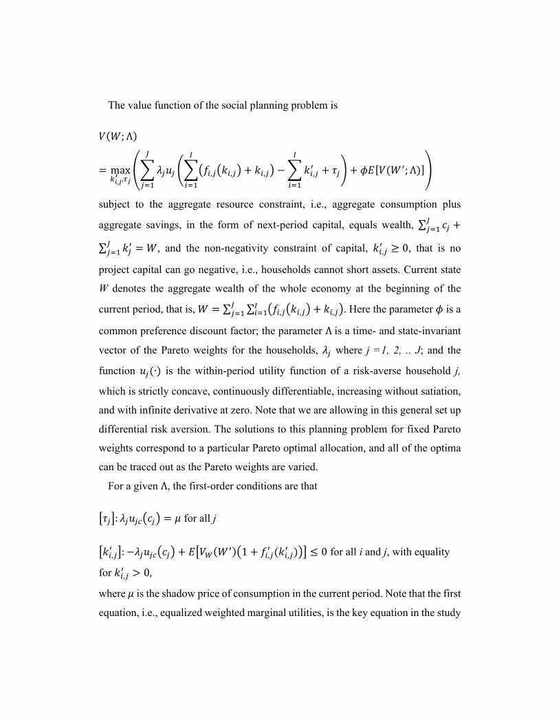
The value function of the social planning problem is

𝑉 𝑊;Λ

= max*(,)F ,G)

𝜆$𝑢$ 𝑓",$ 𝑘",$ + 𝑘",$ − 𝑘",$,9

"6:

+ 𝜏$

9

"6:

J

$6:

+ 𝜙𝐸 𝑉(𝑊,; Λ)

subject to the aggregate resource constraint, i.e., aggregate consumption plus

aggregate savings, in the form of next-period capital, equals wealth, 𝑐$J$6: +

𝑘$,J$6: = 𝑊, and the non-negativity constraint of capital, 𝑘",$, ≥ 0, that is no

project capital can go negative, i.e., households cannot short assets. Current state

W denotes the aggregate wealth of the whole economy at the beginning of the

current period, that is, 𝑊 = 𝑓",$ 𝑘",$ + 𝑘",$9"6:

J$6: . Here the parameter 𝜙 is a

common preference discount factor; the parameter Λis a time- and state-invariant

vector of the Pareto weights for the households, 𝜆$ where j =1, 2, .. J; and the

function 𝑢$(∙) is the within-period utility function of a risk-averse household j,

which is strictly concave, continuously differentiable, increasing without satiation,

and with infinite derivative at zero. Note that we are allowing in this general set up

differential risk aversion. The solutions to this planning problem for fixed Pareto

weights correspond to a particular Pareto optimal allocation, and all of the optima

can be traced out as the Pareto weights are varied.

For a given Λ, the first-order conditions are that

𝜏$ : 𝜆$𝑢$R 𝑐$ = 𝜇 for all j

𝑘",$, : −𝜆$𝑢$R 𝑐$ + 𝐸 𝑉T 𝑊, 1 + 𝑓",$, (𝑘",$, ) ≤ 0 for all i and j, with equality

for 𝑘",$, > 0,

where 𝜇 is the shadow price of consumption in the current period. Note that the first

equation, i.e., equalized weighted marginal utilities, is the key equation in the study

of consumption risk sharing, and it is an integral part of our framework here. The

second equation is a standard Euler equation for investment. Finally, for each 𝑘",$, >

0, the technologies actually chosen, the first-order conditions imply

(1) 1 =WX YZ TF :['(,)

F (*(,)F )

\)])^ R)= 𝐸 WYZ TF

_1 + 𝑓",$, (𝑘",$, ) = 𝐸 𝑚,𝑅",$,

where 𝑚, = WYZ TF

_and 𝑅",$, = 1 + 𝑓",$, (𝑘",$, ).

We focus in part on equation (1) but the other equations are also a key part of the

system. Equation (1) has some important properties. First, 𝑚,, the stochastic

discount factor or the intertemporal marginal rate of substitution, is common across

households and across assets. The model also implies that equation (1) holds for

each of the assets actively allocated to production activity i and run by household

j, for any i and any j. This equation is equivalent to the pricing equation derived in

the Consumption-based Capital Asset Pricing Model (CCAPM) in the finance

literature.6 However, it is important to reiterate that although our empirical

counterpart will be similar to what is derived in the capital asset pricing literature,

the mechanism that delivers the predicted allocation outcome is different. In the

asset pricing literature, households (investors) trade their assets ex ante. Optimally

allocated assets deliver the returns that the households in turn use to finance their

consumption, or reinvest, ultimately maximizing their utility. Although asset

reallocations across households are possible in our model environment, households

do not typically trade their assets ex ante in some markets. The rate of return on an

asset is simply the real yield from holding it. Given asset holdings and given

returns, transfers among households in the economy then give an optimal

consumption allocation, i.e., the consumption allocation under the full risk-sharing

6 For the derivation of this equation from consumer-investor’s maximization problem, see Lucas (1978) and Cochrane

(2001), for example.

regime where the marginal rates of intertemporal substitution are equalized across

households. These inter-household transfers could be through formal securities or

through informal financial markets, namely, gifts and transfers within social

networks.7

Finally, as in the standard asset pricing literature, we decompose expected return

into a risk-free rate and a risk premium. Since 𝐸 𝑚,𝑅",$, = 𝐸 𝑚, 𝐸 𝑅",$, +

𝑐𝑜𝑣 𝑚,, 𝑅",$, , equation (1) can be rewritten as 𝐸 𝑅",$, = 𝛾, + 𝛽fF,"$𝜓fF,where

𝛽fF,"$ = −Rhi fF,j(,)

F

ikl fF , 𝜓fF = ikl fF

X fF , and 𝛾, = :X fF . Note that 𝛽fF,"$ could be

interpreted as the quantity of the risk of the assets used in activity i by household j

that cannot be diversified, i.e., the risk implied by the comovement of the asset

return and the aggregate return. Note that the sign is negative since high returns

mean low marginal utility. Since this risk cannot be diversified away, even in the

full risk-sharing environment, it must be compensated by a risk premium, which is

a product of the quantity of risk and the price of the risk. The price of the risk is in

turn equal to the normalized volatility of the aggregate economy, 𝜓fF. Finally, 𝛾,

is the risk-free rate, 𝑅', , since by definition the covariance of the risk-free rate and

the aggregate economy return is zero.

The intuition behind this optimal allocation is straightforward. An optimal

allocation of assets is a portfolio that delivers an aggregate consumption for the

economy that maximizes the Pareto-weighted expected utility of the households.

This optimal consumption allocation is stochastic, and its distribution is derived

from the distribution of underlying assets in the optimal allocation. Since

households are risk averse, the optimal aggregate consumption represents a tradeoff

7 The Pareto weights, , j = 1, 2,… , J, are implicit parameters in equation (1) as they are arguments in the value function.

Intuitively, the marginal rates of substitution are common across households in any particular optimum but can vary across the many optima, as if moving along a (potentially nonlinear) contract curve. Our general analysis only requires that the risk sharing community be at one fixed social optimum, not at any particular optimal allocation per se. However, when preferences aggregate in a Gorman sense, then the Pareto weights can be dropped from the analysis, and it is as if a social planner were a “stand-in representative consumer” allocating assets among its various “selves”.

between expected return and risk. In the full risk-sharing environment,

idiosyncratic risks are diversified away, and this optimal aggregate consumption

consists of only the aggregate nondiversifiable component. Note that some of the

optimal asset holdings could be zero if they are not needed for the construction of

the portfolio that delivers this optimal aggregate consumption. However, for all of

the assets that are positively allocated, an optimal allocation implies that the

stochastic intertemporal rates of substitution are equalized, i.e., the marginal utility

from the expected returns, net of disutility from risk, from the next period are equal

across these assets. This equalized intertemporal rate of substitution condition

across assets implies that the assets with lower expected return are held in this

optimal portfolio because they are less risky than other assets. Since the only

remaining risk in the full risk-sharing economy is the covariate risk, an optimal

allocation implies the positive relationship between the expected return of the asset

and its covariate, nondiversifiable risk, as represented by the asset’s beta.8

B. A Financial Autarky Benchmark

The second, opposite benchmark case is an economy where households are in

financial autarky and so by definition there is no risk sharing across households.

The underlying environment, in terms of preferences, technologies, and initial

conditions, is of course the same as in the full risk sharing benchmark. In particular,

production technologies deliver returns that are still correlated across households

and production activities. However, households absorb the risk in isolation from

8 Our prediction from the full-risk sharing benchmark should be viewed as a necessary condition for the full risk sharing,

but not a sufficient one. For example, if a household is endowed with a production technology that has returns comoving with the aggregate returns, there will be a positive relationship between expected return and household beta, even when this household is in autarky. However, we have a second necessary condition for optimality: not only is the risk premium determined by comovement with the aggregate, but it is not determined by the idiosyncratic risk as well. This is closely parallel to the consumption risk sharing literature: not only does consumption move with the aggregate but it also does not move with the idiosyncratic income risk.

the rest of the community so that net incoming (or outgoing) transfers, 𝜏𝑗, are zero

for all j. In this benchmark, the value function of each household j is

𝑉$ 𝑊$ = max*(,)F

𝑢$ 𝑓",$ 𝑘",$ + 𝑘",$ − 𝑘",$,9"6:

9"6: + 𝜙𝐸 𝑉$ 𝑊$,

subject to the resource constraint of the household, 𝑊$ = 𝑓",$ 𝑘",$ + 𝑘",$9"6: ,

and the nonnegativity constraint of asset holding, 𝑘",$, ≥ 0.

Operationally, the Euler equation for asset allocation is of the same form as

previous equation (1) for all activities i in which household j chooses to hold and

operate. However, in this environment, the stochastic discount factor would be

specific to household j and not equalized to m, common across all households in

the economy as in the full risk sharing benchmark. Since risk cannot be shared

across households, the total fluctuation of the rate of return on asset for each

household consists of both the household’s idiosyncratic component and the

comovement with the economy-wide return, the latter just another source of risk.

Alternatively speaking, since there is no risk sharing, each household cannot and

does not need to differentiate its idiosyncratic and aggregate risk, as both

components of fluctuation in the rate of return are viewed and treated identically

by the household. In financial autarky, their contribution to the household risk

premium would be the same.

C. Intermediate Cases

Between the full risk sharing benchmark and financial autarky benchmarks lie

various possible intermediate models. These make clear the ways in risk

idiosyncratic income could impact consumption and thus how idiosyncratic risk

can end up in the risk premium. We do not disown either of the previous two

benchmarks above: the full risk sharing benchmarks makes clear the standard ideal

while the financial autarky benchmark makes clear that even if a household were

acting in isolation there would remain risk premia, and with correlated returns, and

both idiosyncratic and aggregate risk would typically enter into these premia. We

view our paper as quantifying how close the villages in our sample are to these

extremes, as with the early, seminal work on consumption risk sharing, and we

anticipate subsequent efforts to fit structural models.9

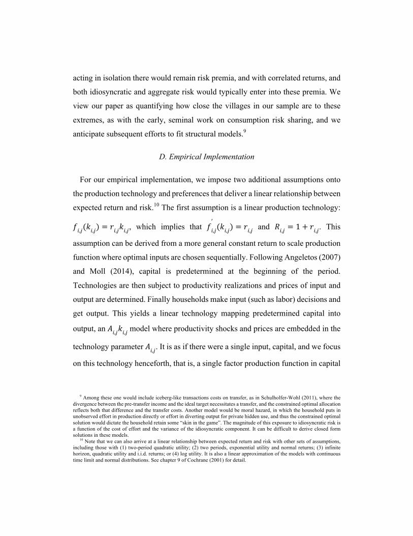
D. Empirical Implementation

For our empirical implementation, we impose two additional assumptions onto

the production technology and preferences that deliver a linear relationship between

expected return and risk.10 The first assumption is a linear production technology:

𝑓𝑖,𝑗(𝑘𝑖,𝑗) = 𝑟𝑖,𝑗𝑘𝑖,𝑗, which implies that 𝑓𝑖,𝑗′(𝑘𝑖,𝑗) = 𝑟𝑖,𝑗 and 𝑅𝑖,𝑗 = 1 + 𝑟𝑖,𝑗. This

assumption can be derived from a more general constant return to scale production

function where optimal inputs are chosen sequentially. Following Angeletos (2007)

and Moll (2014), capital is predetermined at the beginning of the period.

Technologies are then subject to productivity realizations and prices of input and

output are determined. Finally households make input (such as labor) decisions and

get output. This yields a linear technology mapping predetermined capital into

output, an 𝐴𝑖,𝑗𝑘𝑖,𝑗model where productivity shocks and prices are embedded in the

technology parameter 𝐴𝑖,𝑗. It is as if there were a single input, capital, and we focus

on this technology henceforth, that is, a single factor production function in capital

9 Among these one would include iceberg-like transactions costs on transfer, as in Schulholfer-Wohl (2011), where the

divergence between the pre-transfer income and the ideal target necessitates a transfer, and the constrained optimal allocation reflects both that difference and the transfer costs. Another model would be moral hazard, in which the household puts in unobserved effort in production directly or effort in diverting output for private hidden use, and thus the constrained optimal solution would dictate the household retain some “skin in the game”. The magnitude of this exposure to idiosyncratic risk is a function of the cost of effort and the variance of the idiosyncratic component. It can be difficult to derive closed form solutions in these models.

10 Note that we can also arrive at a linear relationship between expected return and risk with other sets of assumptions, including those with (1) two-period quadratic utility; (2) two periods, exponential utility and normal returns; (3) infinite horizon, quadratic utility and i.i.d. returns; or (4) log utility. It is also a linear approximation of the models with continuous time limit and normal distributions. See chapter 9 of Cochrane (2001) for detail.

with random returns. The second assumption is that the value function of the social

planning problem can be well approximated as quadratic in the total assets of the

economy, 𝑉 𝑊 = − 𝜂2𝑊 −𝑊

∗ 2.The derivation in the online Appendix A

shows that under these additional assumptions, our model implies

(2) 𝐸 𝑅$, − 𝑅', = 𝛽$ 𝐸 𝑅-, − 𝑅', ,

where 𝑅$, is the return to household j’s portfolio; 𝑅-, =j(,)F *(,)

Ft(uv

w)uv

*xF , 𝑘-, =

𝑘",$,9"6:

J$6: ; and 𝛽$ is the beta for the return on household j’s assets with respect

to the aggregate market return,

(3) 𝛽$ =Rhi jx

F ,j)F

ikl jxF .

II. Data and the Village Environment

The data used in this study are from the Townsend Thai Monthly Survey, an on-

going intensive monthly survey initiated in 1998 in four provinces of Thailand.

Chachoengsao and Lopburi provinces are semi-urban provinces in a more

developed central region near the capital city, Bangkok. Buriram and Srisaket

provinces on the other hand are rural and located in the less developed northeastern

region by the border of Cambodia. In each of the four provinces, the survey is

conducted in four villages, chosen at random within a given township.11

The analysis presented in this paper is based on 156 months from January 1999

to December 2011, which coincides with 13 calendar years. During this time, there

were salient aggregate shocks and a plethora of repeated idiosyncratic shocks in

11 Given that all four villages in the same province in our data are located in the same township, we use the term province

and township interchangeably in this paper. For details on the Townsend Thai Monthly Survey, see Samphantharak and Townsend (2010).

these village economies. For example, seasonal variation in the amount and timing

of rainfall and temperature can be crucial in rice cultivation. Shrimp ponds were hit

with both diseases as well as restrictions on exports to the EU. At the micro level,

milk cows varied in their productivity, i.e., the flow was quite irregular over time

for a given animal and over the heard.

We include in this study only the households that were present in the survey

throughout the 156 months. Since we compute our returns on assets from net

income generated from cultivation, livestock, fish and shrimp farming, and non-

agricultural business, we also include in this study only the households that

generated income from farm and non-farm business activities for at least 10 months

during the 156-month period (on average about one month per year). In other

words, we drop the households whose income was mainly exclusively from wage

earnings. In the end, there are 541 households in the sample: 129 from (the sampled

township in) Chachoengsao and 140 from Lopburi provinces in the central region,

and 131 from Buriram and 141 from Srisaket provinces in the northeast. Table A.1

in the online appendix presents descriptive statistics of household characteristics.

Table A.2 shows the revenue (gross of cost of production) of the occupations in the

sample.

We use a township as the aggregate market for empirical analysis in this paper

for two reasons. First, the four villages from the same province in our sample are

from the same township and therefore located close to each other. There are likely

economic transactions across these villages. Second, one of the salient features of

the households in the Townsend Thai Monthly Survey is the pervasive kinship

network with extended families. Table A.3 in the online appendix shows that almost

all households in our sample have at least one relative living in the same township.

We use a household as our unit of analysis and consider the return on the

household’s total assets instead of the return on specific assets. As noted earlier, we

consider the total assets as a portfolio that is composed of multiple individual asset

classes (including both financial and fixed assets), and apply the predictions from

our framework to study the risk and return of this portfolio. It is difficult and

arbitrary to assign the percentage use of each asset in each distinct activity.

Imposing additional assumptions on the data to disaggregate assets into

subcategories would likely induce measurement errors that could bias our empirical

analysis.12 The rate of return on assets (ROA) is calculated as household’s accrued

net income divided by household’s total asset (net of liabilities) over the period

from which that the income was generated, i.e., one month in this paper. This is a

conventional financial accounting measure of performance of productive assets.

We use the real accrued net income and the real value of household’s total assets in

the ROA calculation. The real variables were computed using the monthly

Consumer Price Index (CPI) at the regional level from the Bank of Thailand. The

rate is then annualized (multiplied by twelve). We assume that the real risk-free rate

is zero for all of the periods and for all of the townships.13 Table A.4 in the online

appendix presents descriptive statistics of the ROA. The median of the annualized

average ROA was 0.38 percent for Chachoengsao and 1.46 percent for Lopburi in

the central region, and 0.28 percent for Buriram, and 1.99 percent for Srisaket in

the northeast. Excluding land and building structure from total assets, the median

ROA is 1.27 for Chachoengsao and 4.55 for Lopburi in the Central region, and 1.11

for Buriram and 4.23 for Srisaket in the Northeast. The online Appendix C

12 For example, a household that grows rice and also owns a retail shop could use a pick-up truck for both production

activities. Similarly, we do not distinguish well the use of assets for production activity versus consumption activity. This could lead to a downward bias of our estimates on return to assets, as some of the assets that we include in the calculation were not used in production. Samphantharak and Townsend (2012) provide an exercise that classifies total assets into subcategories based on additional assumptions on production and consumption of the households, and analyze the sensitivity of the rate of return. The ROA measure we use here is shown there to be robust.

13 The rationale for the zero risk-free rate is based on the assumption that households have access to storage technology. If the nominal return on stored inventory is the same as inflation rate (which is likely in the case for food crop storage), then the real rate of return is zero. We also perform a robustness check with different risk-free rates. The overall conclusion does not change, which is what we expect because the shift in both excess asset return and excess market return does not affect the covariance between these two variables. Note that in the earlier versions of this paper, we also used alternative calculations of ROA in the analysis, namely, ROA computed only from fixed assets (i.e., excluding financial assets) and nominal ROA (i.e., not adjusted for inflation). Again, the main conclusions did not change. We also used ROA computed from total assets without subtracting liabilities; the overall conclusions were robust (which is sensible, given that liability to asset ratios for most households are relatively small).

describes detailed definition and construction of income, assets, and rate of return,

and provides a discussion on measurement error of the variables.

III. Aggregate Risk and Return on Assets

A. Baseline Specification

In the first stage of our empirical analysis, we compute the asset beta of each

household’s portfolio of assets to get household beta, 𝛽$, for all household j. We

define a township as the aggregate economy and use township average real returns

on assets as aggregate return, 𝑅-, computed as the total net income in the township

divided by the township’s total assets. To avoid the effect of each household’s

return on the township return, for each household we do not include the household’s

own net income and assets in the calculation of its corresponding township return,

i.e., we compute and use instead a leave-out mean. As shown in equation (3), an

asset beta of household j is defined as 𝛽$ =Rhi jx

F ,j)F

ikl jxF , which is the key ratio of

moments we need. Operationally, it is identical and conveniently computed as a

regression coefficient from a simple regression of 𝑅$y, on 𝑅-y, . Specifically, in the

first stage, for each household j we estimate 𝛽$from a time-series regression

(4) 𝑅$y, = 𝛼$ + 𝛽$𝑅-y, + 𝜀$y.

In the second stage, we study the expected return and beta relationship derived

earlier in equation (2). With the assumption that the real return on risk-free asset is

zero, we compute the expected rate of return on assets of household j, 𝐸 𝑅$, .

Empirically, the expected return is computed as a simple time-series average of

monthly rates of return, 𝑅$, =j)|F}

|uv

~, where T is the number of months (156 months

in the baseline specification). We run a cross-sectional regression of household’s

average asset returns on the betas estimated earlier in equation (4) across all

households in each township, one township at a time.

(5) 𝑅$, = 𝛼 + 𝜓𝛽$ + 𝜂$.

With the assumption that the real risk-free rate is zero, the null hypotheses from

equation (5) are that 𝜓 = 𝐸 𝑅-, and that the constant term 𝛼 is zero. Note that we

report the regression coefficient with the standard error corrected for generated

regressor and heteroskedasticity, following Shanken (1992) and Cochrane (2001).

The results in Panel A of Table 1 show that the regression coefficient on

households’ beta is positive for all of the regressions except for the township in

Buriram. We then look at a stronger null hypothesis that 𝜓 = 𝐸 𝑅-, comparing the

magnitude of the estimated regression coefficient 𝜓 with the township expected

return, estimated by the time-series average 𝑅-, =jx|F}

|uv~

. The table also provides

each township’s aggregate expected return. For the two townships in the central

region (Chachoengsao and Lopburi), the regression coefficients are not statistically

different from the township average return (at 10 percent level of significance),

consistent with the prediction from our model. However, the coefficients are

different from the township average return for the township in Srisaket. The zero

constant implication is also satisfied.

[ Insert Table 1 Here ]

To illustrate our results graphically, Figure 1 plots the beta of household j on the

horizontal axis against the expected return on household j’s assets on the vertical

axis for each of the four townships. In general, the figures show a positive

relationship between households’ beta and expected returns. Thus a major

implication of the model is capturing a substantial part of the data. In particular,

higher risk, as measured by the co-movement of household ROA and township

ROA, is associated with higher average return. The positive 𝜓 implication from the

model is pervasive in the data at various levels of aggregation. The more stringent

test of 𝜓 = 𝑅-, is more difficult to satisfy.14 Note that this baseline specification is

subject to some critiques. We now perform robustness checks that address these

issues below.

[ Insert Figure 1 Here ]

B. Time-Varying Risk

Similar to the traditional CAPM in the finance literature, our empirical strategy

assumes that household betas are time-invariant. This assumption allows us to

estimate household betas from time-series regressions. In reality, household betas

could be time-varying. Our sample consists of households engaged in multiple

occupations over the period of 13 years. It is likely that the composition of

household occupations (and hence assets and their associated risks) of some of our

sampled households had changed during this period. Similarly, the expected

aggregate returns 𝐸 𝑅-, could change over time as well, not least from changes in

conditioning factors.

We explore this issue by conducting our empirical analysis on the subsamples of

60 months (5 years) at a time. Specifically, we first estimate household’s 𝛽$ and

expected return using the time-series data from month 5 to month 64 (years 1-5) for

all households. We then perform a similar exercise using the time-series data from

month 17 to month 76 (years 2-6), and so on until the five-year window ends in

14 One may argue that kinship networks are local and operate better at the village or network levels than at the township

level. We present a similar analysis at the village and network levels in the online Appendix D, with the results shown in Tables A.5 and A.6. Overall conclusions remain for most, but not all, of the villages and networks, suggesting that networks may extend beyond the boundary of villages.

month 160 (years 9-13). With all of the estimated 𝛽$� and expected return from all

of the nine subperiods s for all households j, we finally estimate equation (2) using

the pooled household-subperiod data.15 Panel B of Table 1 presents the second-

stage regression results. The table shows that the main prediction of our model still

holds, i.e., higher beta is associated with higher expected (average) return. Note

that allowing for time-varying risk (beta), the prediction from the model is also

satisfied for Buriram. However, the null hypothesis that the constant term is equal

to risk-free rate (assumed to be zero in this paper) is rejected in all of the four

provinces.

C. Aggregate Human Capital

The model presented earlier in this paper implies that a household’s beta captures

all of the aggregate, non-diversifiable risk faced by the household. It is possible that

there is omitted variable bias in the estimation of beta if the average return on

township total assets is not the only determinant of the aggregate risk. Aggregate

wealth, W, in the economy-wide resource constraint likely comes from other assets

in addition to tangible capital held by the households in the economy. As shown in

Table A.2, labor income contributes a large share of household income in our

sample. Omitting human capital from the resource constraint implies that the

economy-wide average return on physical assets (both financial and non-financial)

might not capture the aggregate non-diversifiable risk of the economy. We address

this issue by performing a robustness check. Specifically, we compute an additional

household beta with respect to return to aggregate human capital, proxied by the

15 This empirical strategy is similar to the empirical CAPM literature by Black, Jensen, and Scholes (1972). The difference

is that instead of moving the window month by month, we move the window 12 months (1 year) at a time.

change in aggregate labor income of all households in the economy.16 In particular,

the first-stage time-series regression becomes

𝑅$y, = 𝛼$ + 𝛽$k𝑅-ykF + 𝛽$

�𝑅-y�F + 𝜀$y

where 𝑅-ykF represents the return to aggregate physical (non-human) asset and 𝑅-y

�F

is the return to aggregate human capital. The second-stage cross-sectional

regression is

𝑅$, = 𝛼 + 𝜓k𝛽$k + 𝜓�𝛽$� + 𝜂$.

[ Insert Table 2 Here ]

We then extend our previous empirical analysis to include human capital. The

first four columns of Table 2 show that the regression coefficient of beta with

respect to human capital is not statistically significant in our sample. However, after

controlling for the township return to human capital, the regression coefficients of

beta with respect to total tangible capital (financial, inventory, and fixed assets)

remain positive and significant in all of the four townships.17

D. Time-Varying Stochastic Discount Factor

Similar to the traditional CAPM in the finance literature, parameters that

determine stochastic discount factors are assumed to be time-invariant when we

take the full risk-sharing benchmark to the empirical analysis. In theory, however,

16 This approximation strategy is used in the finance literature by Jagannathan and Wang (1996). Their strategy is based

on a simplified ad hoc assumption that labor income, L, follows an autoregressive process. Therefore, human capital, H, defined as the discounted present value of the labor income stream, is approximated by where r is the discount rate on human capital, and both r and g are taken as constants. In this case, the realized capital-gain part of the rate of return on human capital (not corrected for additional investment in human capital made during the period) will be the growth of the stock of human capital, which is also the realized growth rate in per capita labor income.

17 However, the coefficients on human capital are not significant. This could be due to human capital being measured imprecisely.

they are determined by the shadow price of consumption goods, which likely moves

over time as the aggregate consumption of the economy changes. In order to capture

this time-varying stochastic discount factor, we provide a further robustness check

following a strategy introduced by Lettau and Ludvigson (2001a and 2001b) who

show that these time-varying parameters are functions of aggregate consumption-

wealth ratio. The log consumption-wealth ratio, cay, in turn depends on three

observable variables, namely log consumption, c; log physical (non-human) wealth,

a; and log labor earnings, y. For each household, we compute five betas with respect

to: (1) the aggregate return on tangible capital, 𝑅-ykF ,(2) the aggregate return on

human capital (as computed in the previous analysis), 𝑅-y�F , (3) the predicted value

of 𝑐𝑎𝑦y; (4) the interaction between 𝑅-ykF and 𝑐𝑎𝑦y; and (5) the interaction between

𝑅-y�F and 𝑐𝑎𝑦y.18

(6) 𝑅$y, = 𝛼$ + 𝛽$k𝑅-ykF + 𝛽$

�𝑅-y�F + 𝛽$

Rk�𝑐𝑎𝑦y + 𝛽$Rk�,k 𝑐𝑎𝑦y ∙ 𝑅-yk

F +

𝛽$Rk�,� 𝑐𝑎𝑦y ∙ 𝑅-y

�F + 𝜀$y.

In the final stage we run a cross-sectional regression of households’ average

return on the five betas estimated in equation (6). Namely,

(7𝑅$, = 𝛼 + 𝜓k𝛽$k + 𝜓�𝛽$� + 𝜓Rk�𝛽$

Rk� + 𝜓Rk�,k𝛽$Rk�,k + 𝜓Rk�,�𝛽$

Rk�,� + 𝜂$.)

The results are shown in the last four columns of Table 2. Overall, with the

additional factors in this robustness check, the regression coefficient of market non-

human, physical assets, the main variable from our model, remains positive and

significant for all of the four townships.

18 The online Appendix E provides more information on the estimation procedure of log consumption-wealth ratio.

IV. Idiosyncratic Risk and Return on Assets

The empirical work thus far has abstracted from the presence of idiosyncratic risk

and focused on the implications from the full risk-sharing benchmark. However,

there are reasons why idiosyncratic risk may matter. With any of the departure from

complete risk sharing, the expected return on assets may contain a risk premium

that compensates for residual exposure to idiosyncratic risk.19 We wish to know if

this is true for the households in our sample, and if so, how large that residual

exposure is, quantitatively. In addition, as mentioned earlier, households may be

endowed with production technology that generates the positive relationship

between expected return and beta, even in autarky without risk sharing. We seek to

disentangle this by first estimating idiosyncratic risk in equations (4) and (6)

presented earlier and then quantify the contribution of idiosyncratic risk to the total

return in equations (9) to (11) below.

We follow Fama and Macbeth (1973) and compute idiosyncratic risk from the

variance of the residuals from each of the household’s time-series regressions in

the first step, i.e., the residuals from equation (4).20 This strategy is consistent with

the decomposition of total risk, as measured by the variance of the return on assets,

into aggregate (non-diversifiable) and idiosyncratic (diversifiable) components.

Since equations (4) could be rewritten in a matrix form as 𝑅$y, = 𝐗-y, 𝛽$ + 𝜀$y, we

have

(8) 𝑣𝑎𝑟 𝑅$, = 𝐸 𝛽$,Ω-𝛽$ + 𝑣𝑎𝑟 𝜀$

19 In finance literature, Merton (1987) shows that under-diversified investors demand a return compensation for bearing

idiosyncratic risk. Using the exponential GARCH models to estimate expected idiosyncratic volatilities, Fu (2009) finds a significant and positive relation between the estimated conditional idiosyncratic volatilities and expected returns.

20 In addition to Fama and MacBeth (1973), a recent study by Calvet, Campbell, and Sodini (2007) also uses the same risk decomposition strategy as the one in this paper.

where Ω-is the variance-covariance matrix of the aggregate variables and 𝛽$ is a

vector of the regression coefficients from equation (4). The first term of the right

hand side of equation (8) is therefore the aggregate risk while the second term is

the variance of the residual. We denote this variance of the residual, 𝜎$�, henceforth

simply referred as household sigma, as our measure of household specific

idiosyncratic risk because it summarizes the volatility of the returns that are not

captured by aggregate factor (aggregate return on assets). We emphasize that this

is a household-by-household calculation.

[ Insert Table 3 Here ]

Table 3 presents the decomposition of the total risk faced by the median

household in each of the provinces in our sample, based on equation (8). Panel A

of the table presents the contribution of idiosyncratic risk to the total risk and the

total risk premium, using the beta estimated earlier from the simple specification in

equation (4). Similarly, Panel B uses the betas from the robustness specification in

equation (6). The results shows that a large part of the volatility of the return to

enterprise assets comes from the idiosyncratic component, in all four townships.

The orders of magnitude are large, with the idiosyncratic component capturing at

least 80-90 percent of the risk decomposition of the median households in three out

of four provinces (the exception being Srisaket). Likewise, the aggregate

component can be as low as 2 percent to 20 percent in these three provinces. Of

course, this finding per se is not inconsistent with the model, which allows for

idiosyncratic risk in the technologies. Indeed it is good in the sense that it allows us

to study the impact of aggregate risk, which one might presume from these numbers

to be small, and of idiosyncratic risk, which one might presume to be large. Note

that we can quantify the magnitude of idiosyncratic risk that was diversified from

our estimates of risk and risk premium decomposition. Table 3 also shows that

median households in all provinces except for Srisaket diversified over 90 percent

of their idiosyncratic risk while in Srisaket, the median household was still able to

share almost 80 percent of their idiosyncratic risk. These decompositions are for

each and every household and we thus report as well the interquartile range in each

line.21

We take the first step and add household sigma computed from regressions (4)

and (6), 𝜎$�, as an additional explanatory variable to equations (5) and (7),

respectively.

(9a) 𝑅$, = 𝛼 + 𝜓k𝛽$k + 𝜓�𝜎$� + 𝜂$,

(9b) 𝑅$, = 𝛼 + 𝜓k𝛽$k + 𝜓�𝛽$� + 𝜓Rk�𝛽$

Rk� + 𝜓Rk�,k𝛽$Rk�,k + 𝜓Rk�,�𝛽$

Rk�,� +

𝜓�𝜎$� + 𝜂$.

The results in Table 4 show that, in both baseline and robustness specifications,

higher idiosyncratic risks as measured by household sigma are associated with

higher average returns in all of the four townships.22 Note, however, that the

coefficients for the beta with respect to the market return on physical assets still

remain positive and significant in three of the townships, with Buriram as the only

exception.

[ Insert Table 4 Here ]

Indeed, though both aggregate and idiosyncratic risk are positively correlated

with higher expected return, the “prices” of these risks, i.e., their contribution to

risk premia, is now shown to be different. We compute aggregate and idiosyncratic

21 There are some households that appear to be overcompensated for either idiosyncratic or aggregate risk and have a

contribution of either risk above 100 percent of the total risk premia. 22 Though this violates the exclusion restriction of the full risk sharing benchmark, we are now in a position to compute

risk premium for each type of risk and compare.

risk premia from equations (9a) and (9b) as empirically estimated in Table 4.

Specifically, for the simple specification, we have:

(10a) Aggregate Risk Premium = 𝜓k𝛽$k

(11a) Idiosyncratic Risk Premium = 𝜓�𝜎$� ,

and for the robustness specification, we have:

(10b)Aggregate Risk Premium = 𝜓k𝛽$k + 𝜓�𝛽$� + 𝜓Rk�𝛽$

Rk� + 𝜓Rk�,k𝛽$Rk�,k +

𝜓Rk�,�𝛽$Rk�,�

(11b) Idiosyncratic Risk Premium = 𝜓�𝜎$� .

In the financial autarky benchmark, households would not differentiate the

idiosyncratic component and the aggregate component of the total fluctuation of

the rate of return. In this case, the risk premia from both components should be

proportional to the contribution of each component’s contribution to the total

fluctuation. Panels A.2 and B.2 of Table 3 present the results from the

decomposition of total risk premium of each household (the sum of the aggregate

risk premium and idiosyncratic risk premium) for the simple and the robustness

specifications, respectively. The results show that, with the exception of Buriram,

the contribution of the idiosyncratic risk premia to the total risk premia is lower

than the contribution of idiosyncratic risk to the total risk (as discussed earlier in

Panels A.1 and B.1 of the same table). Specifically, for the robustness specification,

although idiosyncratic risk accounts for 86.5 percent and 89.1 percent of the total

risk of the median households in Chachoengsao and Lopburi, it contributes to only

23.6 percent and 52.9 percent of the total risk premium. Likewise, for the median

household in Srisaket, idiosyncratic risk accounts for 57.2 percent of the total risk

while its premium contributes for only 16.7 percent of the total risk premium. We

also perform a nonparametric statistical test for the difference in medians and find

that the median percentage contribution of idiosyncratic risk to the total risk is

statistically different from the median percentage contribution of idiosyncratic risk

premium to the total risk premium at 1 percent level of significance in all provinces

except for Buriram.23 The pattern for lower and upper quartiles is also similar to

the median. Finally, it is important to note that omitted variables could lead to a

positive relationship between expected return and sigma if a component of

aggregate risk were mistakenly in sigma. However, this would work against us.

Our empirical results suggest the impact of sigma is largely diversified, anyway.

In sum, we cannot treat aggregate and idiosyncratic risks identically when we

analyze the risk and return of household enterprises in developing economies. A

household with high total risk (high variance) may have lower risk premium than

another household if the higher risk is idiosyncratic and diversifiable. Likewise, a

household with low total risk (low variance) could require a higher risk premium if

most of the risk is covariate and nondiversifiable.24

V. Risk Sharing: Connecting the Production Approach to the Consumption

Approach

Reassuringly, our main findings on the production side are largely consistent with

earlier studies on the consumption side that idiosyncratic risk is considerably shared

across households in these villages. Using consumption data from the same sample

as in this paper, Chiappori, Samphantharak, Schulhofer-Wohl, and Townsend

23 One possible explanation for Buriram is that it is the place with the most transition of occupations (toward higher return)

and we have shorter period to use our method. See Pawasuttipaisit and Townsend (2010). 24 To illustrate this point, let us consider two households, A and B, from Lopburi province in our sample. During the

period of this study, A’s main occupation was livestock farming while B grew beans and sunflowers. However, 99 percent of the variance of the rate of return on A’s assets was from the idiosyncratic component while in contrast idiosyncratic risk contributed to only 63 percent for B. Consequently, we find that the risk premium for A, facing mostly diversified risk was only 0.008 (annualized) percentage point while for B with more aggregate risk it was 1.394, despite B’s less volatile return. This example, though deliberately dramatic, is not an outlier. Below we return to an analysis of risk premia and associated characteristics of enterprises that deliver statistically significant variation.

(2013 and 2014) use variation in aggregate shocks to estimate the degree of

heterogeneity in risk tolerance among the households and find evidence for full risk

sharing. Likewise, Karaivanov and Townsend (2014) find that the consumption and

income data of those in family networks is consistent with full risk sharing, though

tied with moral hazard as best fitting models. Kinnan and Townsend (2012) show

that households linked to one another by gifts and loans, and hence indirectly if not

directly connected to outside financial institutions, achieve full risk sharing; in

contrast, isolated households, especially the poor, are vulnerable to idiosyncratic

income risk. Our larger point is that idiosyncratic risk in most of these studies is

partially, though not necessarily completely, insured and this is consistent with

what we are finding in this paper with the data on risk premia from the production

side.

Regarding the actual mechanisms used for smoothing, i.e., financing a deficit or

saving a surplus, households may buy and sell their assets (though this is rare) or

use crop storage inventory (more common). They can also borrow or lend money

formally through financial institutions or informally through village moneylenders,

friends, or relatives. Samphantharak and Townsend (2010) provide quantification

for these various smoothing mechanisms using the same Thai data and document

the role of gifts among social networks.25 Our conceptual framework in this paper

both combines the production and consumption sides, as the first-order conditions

have made clear, and features the role of gifts as the primary smoothing mechanism.

[ Insert Table 5 Here ]

25 The risk sharing implications of networks have been studied in other economies as well. For example, using data from

the randomized evaluation of PROGRESA program in Mexico, Angelucci, De Giorgi, and Rasul (2011) find that members of an extended family share risk with each other but not with households without relatives in the village. They also find that connected households achieve almost perfect insurance against idiosyncratic risk. Recently, Attanasio, Meghir, and Mommaerts (2015) study group risk sharing in extended family networks in the US. They find that majority of shocks to household income are potentially insurable within family networks but they find, in contrast, little evidence that the extended family provides insurance for such idiosyncratic shocks.

We perform further analyses that directly connect production and smoothing

mechanism. For each household, we compute the residual from equation (8) as

month by month idiosyncratic shocks. Then, as reported in Table 5, we regress

household’s net gifts (i.e., gift outflows minus gift inflows) on these idiosyncratic

shocks, controlling for common township-time dummies (capturing aggregate

shocks) and household fixed effects (capturing diverse Pareto weights). Since gifts

could also be disguised in the form of state-contingent loans (as in Udry 1994), we

also regress household’s net lending (i.e, lending minus borrowing), as well as

household’s net gifts plus net lending, on the same set of explanatory variables. The

coefficients are all statistically significant at the 1 percent level. Finally, we also

run the standard risk-sharing regressions with the consumption data (Townsend

1994). Controlling for aggregate shocks and household fixed effects, we regress

monthly consumption on the same idiosyncratic shocks and find a low but

significant coefficient, significant at 5 percent level.

To summarize, the results in Table 5 show that once we control for province-

month fixed effects, which capture the provincial aggregate shocks, household

consumption is positively correlated with household-specific, idiosyncratic shocks.

Thus risk sharing is imperfect and households do bear some of their idiosyncratic

risk. This is consistent with the fact that idiosyncratic risk is showing up in the

idiosyncratic risk premium on the production side. On the other hand, the

coefficient is small, and small in comparison with coefficients on the other

regressions. Most of the movement in idiosyncratic shocks is absorbed by net gifts

and lending across the households. Table 5 can be interpreted to show, via a kind

of normalized covariance decomposition, that on average 40.66/45.52 = 89 percent

of idiosyncratic shocks to rates of return are covered by gifts and net lending, with

the residual onto consumption. Thus the results are quite consistent with the earlier

Table 3.

Finally, we note that the consumption, gift, and lending-borrowing data used in

the analysis in this section are from different modules of the questionnaire than

what we use in the calculation of ROA. Consistency in the empirical findings

reassures us that the main conclusions in this paper are unlikely driven by

measurement error in the data. Of course, there remains the possibility of

measurement error inflating the variance of the idiosyncratic shocks, but

attenuation bias would hit all of the regressions. Thus the relative comparison of

coefficients across regressions remains of interest, confirming the role of social

networks as a key institution in these villages.

VI. Returns Net of Risk Premia

In the development and macroeconomics literatures mentioned earlier in the

introduction, rates of return on assets are usually used as a measure of performance,

the productivity of a firm or a household enterprise. These returns to assets however

typically do not take into account that different household enterprises are involved

in different risks and so that higher average returns could result from compensation

for higher risk and not productivity.26

The framework in this paper gives us a practical way to compute the risk premia

that contribute to the return on assets and hence the residual return, after adjusting

for the premium, as in the example just given. In the conventional CAPM context,

Jensen (1967) argues that intercepts 𝛼$ in equations (6) can be interpreted as the

abnormal return of an asset, and financial analysts use Jensen’s alpha as a measure

26A comparison of two farming households in Srisaket province, C and D, from our sample illustrates this argument. Their

main crops were rice and cassava, respectively. During the period of our study, the average annualized monthly real rate of return on assets for C was 9.06 percent while it was only at 3.93 percent for D. However, C’s higher return was largely due to the higher risk and the types of risk it faced. First, C was engaged in production activity whose return fluctuated more than D: the variance of the rate of return for C was 2.26 times higher than that of D. Second, while 70 percent of the total risk faced by C was idiosyncratic and could be (partially) diversified away, the diversifiable risk component accounted for 89 percent for D. As a result, the risk premium of C was 8.25 percentage points while it was only 1.11 percentage points for D. In the end, C actually had a lower return net of risk, i.e., after subtracting risk premia, a net of 0.81 percent, in comparison to D at 2.82 percent.

of performance of an asset or a fund manager. We follow this tradition, thinking of

𝛼$as how well household j manages its assets in generating income in excess of

risk-free rate adjusting for measured risk premia.

[ Insert Figure 2 Here ]

Figure 2 shows the histograms comparing the return on assets that is not adjusted

for risks with the return adjusted for both aggregate and idiosyncratic (based on the

robustness specification). Though risk adjusted returns are naturally shifted to the

left, other aspects of the distribution also change. The modes receive high mass

consistently in the risk-adjusted returns. Further in two provinces the adjusted

returns have more mass in the left tail, and in the other two provinces, in the right

tail. The overall point is that the distributions of the rate of return do change when

we adjust for risks, as evident from the differences in the skewness and the kurtosis

of the returns. Table A.7 in the online appendix presents selected descriptive

statistics of household alpha.

VII. Household Characteristics Associated with Risk Exposure and Return

on Assets

Figure 3 presents a scatter plot displaying for each household its aggregate risk

premium and idiosyncratic risk premium. The figure shows that some households

in our sample were exposed to both high aggregate and idiosyncratic risks (those in

the upper-right corner) while many faced little of both risks (those in the lower-left

corner). Still, there are a large number of households that were mainly exposed to

one type of risk, but not the other (those in the upper-left and in the lower-right

corners).27

27 Figure 3 also presents two salient findings from our sample. First, there is a positive correlation between aggregate risk

premium and idiosyncratic risk premium (the correlation coefficient is 0.49 and statistically significant at 1 percent). Second,

[ Insert Figure 3 Here ]

Table 6 presents correlations in the data, with different measures of return and

risk of assets as the dependent variable and household’s initial wealth and other

demographic characteristics on the right hand side. Specifically, Panel A presents

regression results when we us the simple measured rate of return on assets (not

adjusted for risk) as the dependent variable. In three out of four provinces, we find

that poor households (as measured by initial wealth) tend to have higher average

return on assets. This result might prompt us to conclude that households in these

provinces are financially constrained. However, the results in Panel B reveal a

different story. Once adjusted for risk, poorer households in the central region tend

to have a lower return on assets while there is no relationship between wealth and

return on assets for the two provinces in the northeast.

The explanation for these findings is shown in Panels C and D where we examine

the relationship between household characteristics and household beta (aggregate

risk with respect to the market return on physical assets) and household sigma

(idiosyncratic risk). The results highlight the heterogeneity in the risk exposure of

households in our sample. Controlling for household demography, poorer

households tend to be more involved with risky activities, both aggregate (in 3 out

of 4 provinces) and idiosyncratic (in all 4 provinces). We also find that households

with younger, less educated, and male head tend to have more exposure to both

aggregate and idiosyncratic risks (although specific results vary across provinces).

[ Insert Table 6 Here ]

there is a large portion of our sampled households with low risk (those near the origin in Figure 3). In particular, there is variation in aggregate risk premium while the idiosyncratic part is near zero. This produces a cluster of points on the horizon axis.

One might well ask, what is the mechanism that households choose to make their

income smooth or risky? We further explore the sources of this household risk

exposure (results not shown here). Using the data on the shares of household total

revenue from each production activity as well as the data on each household’s main

occupation (cultivation, livestock, fish and shrimp farming, and non-farm

business), we find that cultivation is associated with the highest aggregate and

idiosyncratic risk (these are statistically significant at 1 percent). Cultivation is

common in our sample (hence aggregate risk), but at the same time there is

heterogeneity in the variability of returns within cultivation (hence idiosyncratic

risk). Finally, we find that poorer households are more likely to participate in

cultivation (again, statistically significant at 1 percent). Note also that this finding

is unlikely driven by the difference in risk preferences between rich and poor

households as Chiappori, Samphantharak, Schulhofer-Wohl, and Townsend (2013

and 2014), using data from the same household survey as this paper, find that risk

aversion was not correlated with household wealth. This is related to the underlying

force of the full risk sharing benchmark, under which production and consumption

activities are separated.

The result shows how easily one could misinterpret data, if one did not adjust for

risk. One might have impression that relatively poor households have high returns

on assets (as shown in Panel A for all of the provinces except for Lopburi) and thus

suffer from financial constraints. The results here show that the reason why these

poor households have a higher simple rate of return to their business enterprises is

from the fact that they take more risk in their production activities and get

compensated accordingly. Controlling for risks, household enterprises of the poor

in the northeast are not productively different those of the rich, while the poor in

the central region tend to have lower return on assets that the rich. Thus some poor

households in our sample, those of the central region, do seem constrained, but not

in the usual, stereotypical sense. Poor households seem limited in their choices of

production activities, as if constrained away from the activities that have high return

net of risk premia and are available largely for richer households. Our findings

suggest that there exist obstacles for the poor to leave their current occupation rather

than funding the current one. Our finding is similar to Rampini and Viswanathan

(2016) who find that household risk management is incomplete and increasing in

household net worth and income.28 The limitation of poor households to diversify

idiosyncratic income risk is in contrast to Morduch (1995), who finds that poor

households in villages in India that have limited ability to smooth consumption ex

post and tend to choose production activities that give them smoother income ex

ante.

VIII. Conclusion and Policy Implications

We study the risk and return of farm and non-farm business enterprises in village

economies. Using data from the Townsend Thai Monthly Survey, we find that

although idiosyncratic risk is the dominant factor in the total risk, it is diversified

away to a large extent, and so bears a low risk premium. In contract, aggregate risk

cannot be diversified away and likewise it captures a much larger share of the total

risk premia. Our results, using data on the rates of return from production side, are

parallel to those in the consumption risk sharing literature that uses income and

consumption as key variables. We also provide an analysis that jointly makes use

of production and consumption panel data, at the level of individual households

over time. Our study has important policy implications: when comparing business

across sectors or production across different activities, the adjustments for

28 Our findings do not necessarily contradict existing literature that analyzes the gross rate of return, unadjusted for risk

premia, and financial constraints. If all households are in the same occupation or a sector that has identical aggregate risk, and if idiosyncratic risk is fully diversified, then actual net returns, adjusted for risk, are simply a downward shifted version of the unadjusted returns. Some on the right tail of this distribution may have high net returns and thus may be constrained. More generally, however, with different occupations and differential exposure to risk, high returns on the right tail of the distribution may be simply the compensation for high risk. Likewise, high rates of growth of net worth for poor households with high rates of return does not necessarily indicate the presence of financial constraints, as those with high expected returns, however risky, will on average as a group, experience high growth.

aggregate and idiosyncratic risks can vary and there is potentially little association

between high returns and underlying productivity.

Appendix

Appendix A: Derivation of Empirical Specification

Due to the first assumption on linear production technology, equation (1) also

holds for any of the portfolios constructed by any combinations of the assets 𝑘",$,

for all i and all j. If we consider a household as our unit of observation, equation

(1) implies that 1 = 𝐸 𝑚,𝑅$, , where 𝑅$, =�(,)F j(,)

Ft(uv

�(,)Ft

(uv. In other words, 𝑅$, is the

weighted average return to the portfolio of the assets operated by household j,

where the weights are the shares of each asset in household j’s portfolio. This

insight allows us to study the risk and return of a household’s portfolio of assets

instead of the risk and return of each individual asset. This implication is especially

important in the empirical study where the classification of asset types and the

income stream from each asset is problematic, as one asset may be used in various

production activities or various types of assets are used jointly in a certain

production activity.

The second assumption that the value function of the social planning problem can

be well approximated as quadratic in the total assets of the economy implies that at

𝑊,,

(A1)𝑉T 𝑊, = −η 𝑊, −𝑊∗ = −η 𝑅",$, 𝑘",$,9"6:

J$6: −𝑊∗ = −η 𝑅-, 𝑘-, −

𝑊∗ ,

where 𝑅-, =j(,)F *(,)

Ft(uv

w)uv

*xF and 𝑘-, = 𝑘",$,9

"6:J$6: . The first-order conditions

from the value function (A1) imply

𝑚, = −W� jxF *x

F �T∗

_= W�T∗

_− W�*x

F

_𝑅-, ,

(A2) 𝑚, = 𝑎 − 𝑏𝑅-, ,

where a and b are implicitly defined. Next, combining equation (A2) with the Euler

equation derived earlier,

𝐸 𝑅",$, = 𝛾, −Rhi k��jx

F ,j(,)F

ikl k��jxF ∙ ikl k��jx

F

X k��jxF

𝐸 𝑅",$, = 𝛾, +Rhi(jx

F ,j(,)F )

ikl(jxF )

∙ �∙ikl(jxF )

k��∙X[jxF ]

(A3) 𝐸 𝑅",$, = 𝛾, + 𝛽",$ ∙ 𝜓,

which is a linear relationship between the expected return of an asset, 𝐸 𝑅",$, its

nondiversifiable risk as measured by the comovement with the aggregate return,

𝛽",$, and the price of the nondiversifiable risk, 𝜓. Note again that equation (A3)

holds for any assets or portfolios of assets, including the market portfolio, M, and

the risk-free asset, f. Since 𝛽- = 1 and 𝛽' = 0, equation (A3) also implies that 𝛾, =

𝑅', and 𝜓 = E 𝑅-, − 𝑅",$, . In other words, the price of the aggregate,

nondiversifiable risk is equal to the expected return on the market portfolio in

excess of the risk-free rate. This condition, presented in equation (A3), is equivalent

to the relationship between risk and expected return derived in the traditional

Capital Asset Pricing Model (CAPM) in asset pricing literature. Finally, as

discussed earlier, equation (A3) also holds for any of the portfolios constructed by

any combinations of the assets for any i and any j because the production

technologies are assumed to be linear in capital. In other words, for each household

j, we can derive equation (2) as

(2) 𝐸 𝑅$, − 𝑅', = 𝛽$ ∙ 𝐸 𝑅-, − 𝑅', ,

where 𝑅$, is the return to household j’s portfolio and 𝛽$ is the beta for the return on

household j’s assets with respect to the aggregate market return,

(3) 𝛽$ =Rhi(jx

F ,j)F)

ikl(jxF )

.

Also, note that common quadratic utility functions do Gorman aggregate and we

can drop the reference to Pareto weights. Also, the quadratic utility function is not

the only setting that delivers this result.

Appendix B: Descriptive Statistics

[ Insert Tables A1-A4 Here ]

Appendix C: Construction of Income, Assets, and Rate of Return

Net Income: Income is accrued household enterprise income, which is the

difference between the enterprise total revenue and the associated cost of inputs

used in generating that revenue. Revenue is realized at the time of sale or disposal.

Associated cost could be incurred earlier, in the periods before the sale or disposal

of outputs. Total revenue includes the value of all outputs the household produces

for sale (in cash, in kind, or on credit), own consumption (imputed value), or given

away. Revenue also includes rental income from fixed assets. Revenue does not

include wages earned outside the household or gifts and transfers received by the

household. Cost includes the value of inputs used in the production of the outputs,

regardless of the method of their acquisition, i.e., purchase (in cash, in kind, or on

credit) or gifts from others or transfers from government. Costs includes the wage

paid to labor provided by non-household members as well as imputed compensation

to the labor provided by household members.29 Cost includes all utility expenses of

the household regardless of the purposes of their uses and also includes depreciation

of fixed assets.

29 For the detailed procedure how we impute the compensation to household's own labor, See Samphantharak and

Townsend (2010).

Total Assets: Assets include all assets, i.e., fixed assets, inventories, and financial

assets. Fixed assets are surveyed in the Agricultural Assets, Business Assets,

Livestock, Household Assets, and Land Modules of the survey. In the Agricultural

Assets Module, fixed assets include walking tractor, large four-wheel tractor, small

four-wheel tractor, aerator, machine to put in seeds and pesticides, machine to mix

fertilizer and soil, sprinkler, threshing machine, rice mill, water pump, rice storage

building, other crop storage building, large chicken coop, other buildings for

livestock, and other buildings. In the Household Assets Module, assets include car,

pick-up truck, long-tail boat with motor, large fishing boat, bicycle, air conditioner,

regular telephone, cellular telephone, refrigerator, sewing machine, washing

machine, electric iron, gas stove, electric cooking pot, sofa, television, stereo, and

VCR.30 Due to the variety in non-agricultural businesses, in the Business Module,

we do not list the specific name of the assets, but instead ask the household to report

the fixed assets they use in their business enterprises. In the Land Module, assets

include land and building at acquisition value, the value of land and building

improvement, and the appreciation of land when major events occurred (such as an

addition of new public roads). In all of the modules, assets that are not explicitly

listed but have value more than 2,000 baht are also asked and included. We also

adjust the value of fixed assets with monthly depreciation. Inventories include raw

material, work in progress, finished goods for cultivation, fish and shrimp farming,

livestock activities (such as milk and eggs), and manufacturing non-farm

businesses. For merchandizing non-farm businesses, inventories are mainly goods

for resale. Animals from the Livestock Inventory Module, which include young

meat cow, mature meat cow, young daily cow, mature dairy cow, young buffalo,

30 Note that we decide to include all household assets in our calculation. This is mainly because some of these assets were

used by the households in their production activities as well and it would be arbitrary to include certain household assets while excluding others. However, the value of these assets was relatively small compared to the value of total assets (which was largely determined by land and other fixed assets). See Samphantharak and Townsend (2012) for the sensitivity analysis of ROA on household assets.

mature buffalo, young pig, mature pig, chicken, and duck, are accounted as either

inventories or fixed assets, based on their nature. Financial assets include cash,

deposits at financial institutions, other lending, and net ROSCA position. These line

items are computed from the Savings Module, the Lending Module, and the

ROSCA Module. The stock of cash is not asked directly but can be imputed from

questions about each and every transaction that each household had since the last

interview. Finally, the total asset used in the calculation of rate of return is net of

liabilities. We use the information from the Borrowing Module to calculate the

household’s stock of total liabilities.

Rate of Return: The rate of return on assets (ROA) is defined as household’s

accrued net income divided by household’s average total assets (net of total

liabilities) over the period from which that the income was generated, i.e., one

month in this paper. The average total asset is the sum of total assets at the

beginning of the month and total assets at the end of the month, divided by two.

Discussion on Measurement Errors: For the aggregate risk, the positive

relationship between beta and expected (or mean) return could be driven by

measurement errors if the measurement errors of household ROAs are positively

correlated with the measurement errors of the aggregate ROA. However, for most

production activities, we use direct answers on revenue from those production

activities from each household to compute that household’s ROA. Constructing

price indices from these data reveals that prices in a given month can vary

considerably over households. This may be due in part to the fact that we did not

try to distinguish within village versus farm gate prices, i.e., we have revenue and

price at the point of sale, wherever that might be. Actual and imputed wages also

vary enormously over households at a point in time. There are also likely

measurement errors in idiosyncratic returns but detailed studies of rice production

show that yields can be explained beyond rainfall by measured differences in soil

moisture, soil type, elevation, and timing of rain, which are all household specific,

and hence much of the heterogeneity across households is real and not necessary

measurement error (Tazhibayeva and Townsend 2012). Of course, some

measurement errors are intrinsic to any survey. However, as we will discuss later

in this paper, our findings from the analyses that use the data from the production

modules of the survey are largely consistent with the findings from the

consumption, gifts, and loan modules of the same survey. This independence across

modules reassure us that the main conclusions in this paper are unlikely driven by

measurement error in the data.

Appendix D: Alternative Definitions of the Aggregate Economy

One may argue that kinship networks are local and operate better at the village

or network levels than at the township level. Table A.5 reports the second-stage

regression results when we use villages as aggregates. Despite the smaller number

of observations, the results show that the regression coefficient of household beta

is significantly positive at 10 percent (or lower) level of significance for 9 of the 16

villages in our sample, with the only exception of all four villages in Buriram

province, two villages in Lopburi, and one village in Chachoengsao. The result also

shows that we cannot reject the null hypothesis that 𝜓 = 𝑅- at 10 percent level of

significance for 5 out of those 9 villages in the sample (Village 7 in Chachoengsao;

Village 4 in Lopburi; and Villages 6, 9, and 10 in Srisaket).

[ Insert Tables A5 Here ]

We also perform a similar analysis at the network level. In order to analyze the

risk and return at the network level, we construct kinship network maps for the

households in the Townsend Thai Monthly Survey. Specifically, for each of the

relatives of the household head and the spouse (parents and siblings of the head,

parents and siblings of the spouse, and their children) who was still alive and lived

within the village, the survey recorded which building structure as recorded in the

initial census he or she lived. With this information, we constructed a kinship

network map for each village by drawing a link between two households that were

family-related related. We present in Table A.6 the regressions using network as

our definition of aggregate economy. We present only the results for the networks

with more than 15 households. There are nine of them. All are from different

villages (four from Lopburi in the central region; two from Buriram and three from

Srisaket in the northeast). Table A6 shows that the regression coefficient of

household beta is significantly positive for 5 of the 9 networks. For 2 of the 9

networks, we however cannot reject the null hypothesis that the regression

coefficient is equal to the network’s average return (Networks 602 and 902 in

Srisaket).

[ Insert Tables A6 Here ]

Appendix E: Time-Varying Stochastic Discount Factor

To show that the consumption-wealth ratio summarizes the expectation of future

returns, Lettau and Ludvigson (2001a) start from the resource constraint in period

t analogous to what presented in Section I of this paper, 𝑊y[: = (1 + 𝑟-,y[:) ∙

(𝑊y − 𝐶y), where 𝑊y, 𝐶y, and 𝑟-,y are wealth, consumption, and market rate of

return in period t. Following Campbell and Mankiw (1989), the log-linear

approximation of this constraint yields 𝑐y − 𝑤y ≈ 𝐸y 𝜌�� (𝑟-,y[� − Δ𝑐y[�)��6:

where 𝜌� =T��T

or the steady-state investment to wealth ratio. Define 𝑐𝑎𝑦y = 𝑐y −

𝑤y = 𝑐y − 𝜔𝑎y − (1 − 𝜔)𝑦y, where a is the share of physical wealth in total

wealth. Since we do not observe the share of non-human wealth, 𝜔, we cannot

directly compute the log consumption to wealth ratio, 𝑐𝑎𝑦y. Instead, we follow

Lettau and Ludvigson (2001a) and obtain the value of 𝑐𝑎𝑦y from 𝑐𝑎𝑦y = 𝑐y∗ −

𝜔𝑎y∗ − 𝜃𝑦y∗ − 𝛿, where the starred variables are the observed quantities from our

data and the hatted values are the estimated coefficients from the township time-

series regression 𝑐y∗ = 𝛿 + 𝜔𝑎y∗ + 𝜃𝑦y∗ + 𝜀y.

Appendix F: Risk-Adjust Return

[ Insert Table A7 Here ]

REFERENCES

Angeletos, George-Marios. “Uninsured idiosyncratic investment risk and aggregate

saving,” Review of Economic Dynamics 10(1), 2007.

Angelucci, Manuela; Giacomo de Giorgi; and Imran Rasul. “Insurance and

Investment within Family Networks,” Working Paper, 2011.

Asker, John; Allan Collard-Wexler; and Jan De Loecker. “Dynamic Inputs and

(Mis)Allocation.” Journal of Political Economy 122(5): 1013-1063, 2014.

Attanasio, Orazio; Costas Meghir; and Corina Mommaerts. “Insurance in Extended

Family Networks,” NBER Working Paper No. 21059, April 2015.

Banerjee, Abhijit, Dean Karlan and Jonathan Zinman. "Six Randomized

Evaluations of Microcredit: Introduction and Further Steps." American Economic

Journal: Applied Economics, 7(1): 1-21, 2015.

Bartelsman, Eric; John Haltiwanger; and Stefano Scarpetta. “Cross-Country

Differences in Productivity: The Role of Allocation and Selection.” American

Economic Review 103(1): 305-334, 2013.

Beaman, Lori; Dean Karlan; Bram Thuysbaert; and Christopher Udry. “Selection

into Credit Markets: Evidence from Agriculture in Mali,” Working Paper,

February 2015.

Black F., M.C. Jensen, and M. Scholes. "The Capital Asset Pricing Model: Some

Empirical Tests" in Jensen, M.C., ed., Studies in the Theory of Capital Markets,

Praeger, 1972.

Buera, Francisco J. and Yongseok Shin. "Financial Frictions and the Persistence of

History: A Quantitative Exploration," Journal of Political Economy 121(2),

2013.

Calvet, Laurent; John Y. Campbell; and Paulo Sodini. “Down or Out,” Journal of

Political Economy 115, 2007.

Campbell, John Y. “Consumption-Based Asset Pricing,” Chapter 13 in Handbook

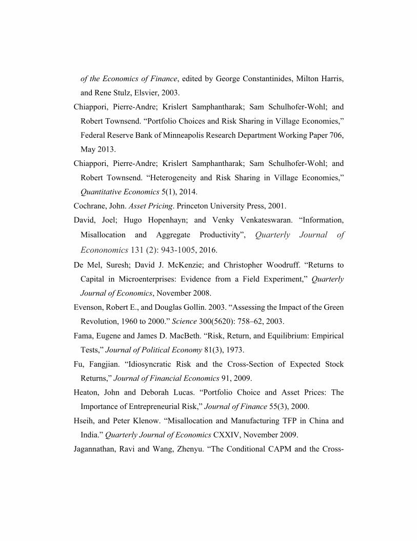
of the Economics of Finance, edited by George Constantinides, Milton Harris,

and Rene Stulz, Elsvier, 2003.

Chiappori, Pierre-Andre; Krislert Samphantharak; Sam Schulhofer-Wohl; and

Robert Townsend. “Portfolio Choices and Risk Sharing in Village Economies,”

Federal Reserve Bank of Minneapolis Research Department Working Paper 706,

May 2013.

Chiappori, Pierre-Andre; Krislert Samphantharak; Sam Schulhofer-Wohl; and

Robert Townsend. “Heterogeneity and Risk Sharing in Village Economies,”

Quantitative Economics 5(1), 2014.

Cochrane, John. Asset Pricing. Princeton University Press, 2001.

David, Joel; Hugo Hopenhayn; and Venky Venkateswaran. “Information,

Misallocation and Aggregate Productivity”, Quarterly Journal of

Econonomics 131 (2): 943-1005, 2016.

De Mel, Suresh; David J. McKenzie; and Christopher Woodruff. “Returns to

Capital in Microenterprises: Evidence from a Field Experiment,” Quarterly

Journal of Economics, November 2008.

Evenson, Robert E., and Douglas Gollin. 2003. “Assessing the Impact of the Green

Revolution, 1960 to 2000.” Science 300(5620): 758–62, 2003.

Fama, Eugene and James D. MacBeth. “Risk, Return, and Equilibrium: Empirical

Tests,” Journal of Political Economy 81(3), 1973.

Fu, Fangjian. “Idiosyncratic Risk and the Cross-Section of Expected Stock

Returns,” Journal of Financial Economics 91, 2009.

Heaton, John and Deborah Lucas. “Portfolio Choice and Asset Prices: The

Importance of Entrepreneurial Risk,” Journal of Finance 55(3), 2000.

Hseih, and Peter Klenow. “Misallocation and Manufacturing TFP in China and

India.” Quarterly Journal of Economics CXXIV, November 2009.

Jagannathan, Ravi and Wang, Zhenyu. “The Conditional CAPM and the Cross-

Section of Expected Returns,” Journal of Finance 51, 1996.

Jensen, Michael C. “The Performance of Mutual Funds in the Period 1945-1964.”

Journal of Finance 23(2): 389-416, 1967.

Karaivanov, Alexander, and Robert M. Townsend. “Dynamic Financial

Constraints: Distinguishing Mechanism Design from Exogenously Incomplete

Regimes,” Econometrica, 2014.

Karlan, Dean; Robert Osei; Isaac Osei-Akoto; and Christopher Udry. “Agricultural

Decisions after Relaxing Credit and Risk Constraints,” Working Paper, Yale

University, 2013.

Kartashova, Katya. "Private Equity Premium Puzzle Revisited." American

Economic Review 104(10): 3297-3334, 2014.

Kinnan, Cynthia and Robert M. Townsend. “Kinship and Financial Networks,

Formal Financial Access and Risk Reduction,” American Economic Review

Papers and Proceedings 102, 2012.

Lettau, Martin and Sydney Ludvigson. “Consumption, Aggregate Wealth, and

Expected Stock Returns” Journal of Finance, 2001a.

Lettau, Martin and Sydney Ludvigson. “Resurrecting the (C)CAPM: A Cross-

Sectional Test When Risk Premia Are Time-Varying” Journal of Political

Economy 109, 2001b.

Lucas, Robert E., Jr. “Asset Prices in an Exchange Economy,” Econometrica 46,

1978.

Mankiw, N. Gregory and Stephen P. Zeldes. “The Consumption of Stockholders

and Nonstockholders,” Journal of Financial Economics 29, 1991.

McKenzie, David and Christopher Woodruff. “Experimental Evidence on Returns

to Capital and Access to Finance in Mexico” World Bank Economic Review

22(3), 2008.

Midrigan, Virgiliu and Daniel Xu. “Finance and Misallocation: Evidence from

Plant-Level Data,” American Economic Review 104 (2): 422-458, 2014.

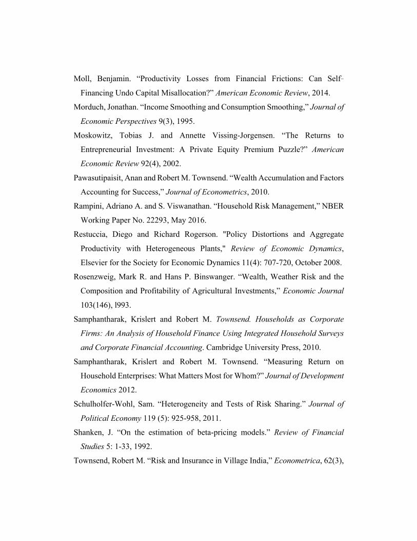
Moll, Benjamin. “Productivity Losses from Financial Frictions: Can Self‐

Financing Undo Capital Misallocation?” American Economic Review, 2014.

Morduch, Jonathan. “Income Smoothing and Consumption Smoothing,” Journal of

Economic Perspectives 9(3), 1995.

Moskowitz, Tobias J. and Annette Vissing-Jorgensen. “The Returns to

Entrepreneurial Investment: A Private Equity Premium Puzzle?” American

Economic Review 92(4), 2002.

Pawasutipaisit, Anan and Robert M. Townsend. “Wealth Accumulation and Factors

Accounting for Success,” Journal of Econometrics, 2010.

Rampini, Adriano A. and S. Viswanathan. “Household Risk Management,” NBER

Working Paper No. 22293, May 2016.

Restuccia, Diego and Richard Rogerson. "Policy Distortions and Aggregate

Productivity with Heterogeneous Plants," Review of Economic Dynamics,

Elsevier for the Society for Economic Dynamics 11(4): 707-720, October 2008.

Rosenzweig, Mark R. and Hans P. Binswanger. “Wealth, Weather Risk and the

Composition and Profitability of Agricultural Investments,” Economic Journal

103(146), l993.

Samphantharak, Krislert and Robert M. Townsend. Households as Corporate

Firms: An Analysis of Household Finance Using Integrated Household Surveys

and Corporate Financial Accounting. Cambridge University Press, 2010.

Samphantharak, Krislert and Robert M. Townsend. “Measuring Return on

Household Enterprises: What Matters Most for Whom?” Journal of Development

Economics 2012.

Schulholfer-Wohl, Sam. “Heterogeneity and Tests of Risk Sharing.” Journal of

Political Economy 119 (5): 925-958, 2011.

Shanken, J. “On the estimation of beta-pricing models.” Review of Financial

Studies 5: 1-33, 1992.

Townsend, Robert M. “Risk and Insurance in Village India,” Econometrica, 62(3),

1994.

Udry, Christopher. “Risk and Insurance in a Rural Credit Market: An Empirical

Investigation in Northern Nigeria,” Review of Economic Studies 61, 1994.

Udry, Christopher and Santosh Anagol. "The Return to Capital in Ghana,"

American Economic Review 96(2): 388-393, 2006.

Vissing-Jorgensen, Annette. “Asset Market Participation and the Elasticity of

Intertemporal Substitution.” Journal of Political Economy, August 2002.

Vissing-Jorgensen, Annette and Orazio Attanasio. “Stock Market Participation,

Inter-temporal Substitution, and Risk Aversion,” American Economic Review 36,

2003.

FIGURE 1. RISK AND RETURN: TOWNSHIP AS MARKET

Notes: Unit of observation is household. There are 129 households in Chachoengsao, 140 in Lopburi, 131 in Buriram, and 141 in Srisaket. The fitted lines correspond to regression results presented in Columns (1) to (4) in Table 1.

-10

010

2030

Mea

n RO

A

0 2 4 6 8 10Beta

(mean) roa Fitted values

Chachoengsao

-20

-10

010

20M

ean

ROA

-2 0 2 4 6Beta

(mean) roa Fitted values

Lopburi

-10

-50

510

Mea

n RO

A

-2 0 2 4 6Beta

(mean) roa Fitted values

Buriram

-20

-10

010

20M

ean

ROA

0 2 4 6 8Beta

(mean) roa Fitted values

Srisaket

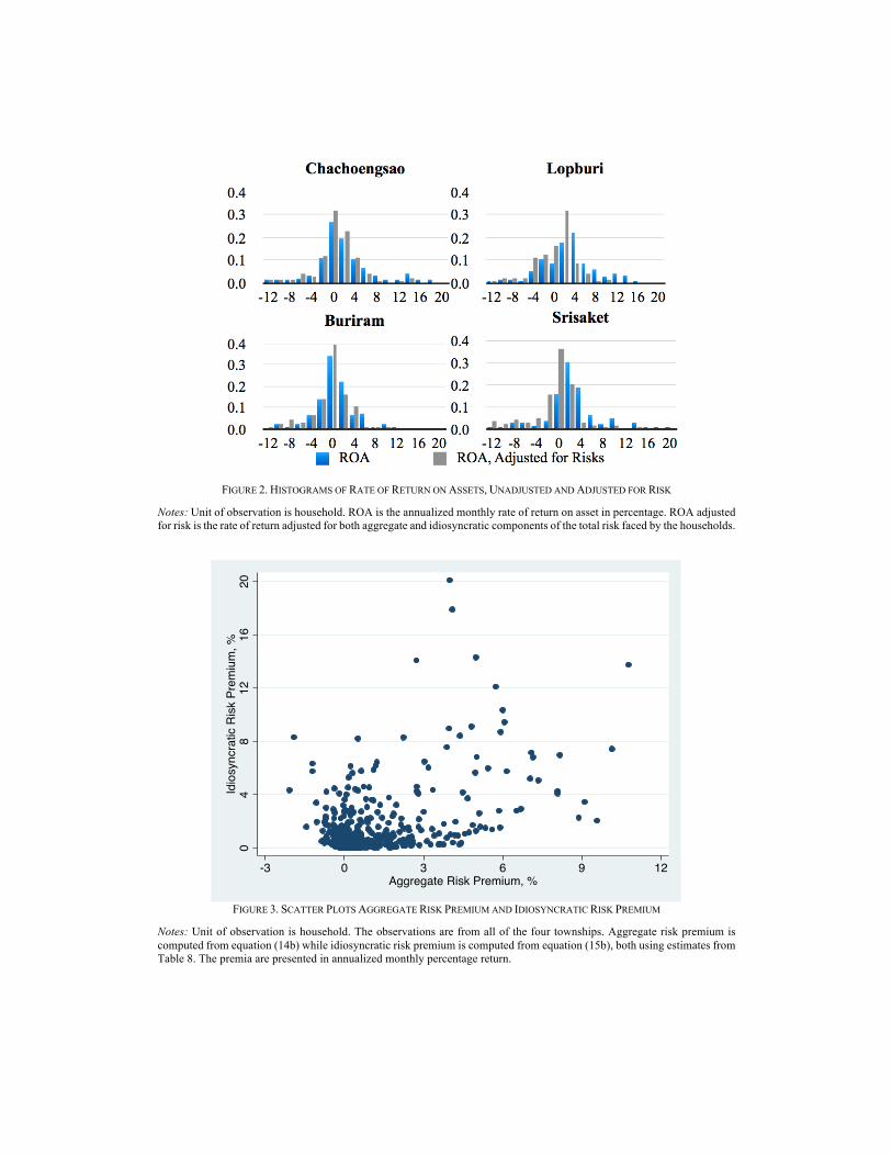
FIGURE 2. HISTOGRAMS OF RATE OF RETURN ON ASSETS, UNADJUSTED AND ADJUSTED FOR RISK

Notes: Unit of observation is household. ROA is the annualized monthly rate of return on asset in percentage. ROA adjusted for risk is the rate of return adjusted for both aggregate and idiosyncratic components of the total risk faced by the households.

FIGURE 3. SCATTER PLOTS AGGREGATE RISK PREMIUM AND IDIOSYNCRATIC RISK PREMIUM

Notes: Unit of observation is household. The observations are from all of the four townships. Aggregate risk premium is computed from equation (14b) while idiosyncratic risk premium is computed from equation (15b), both using estimates from Table 8. The premia are presented in annualized monthly percentage return.

04

812

1620

Idio

sync

ratic

Ris

k Pr

emiu

m, %

-3 0 3 6 9 12Aggregate Risk Premium, %

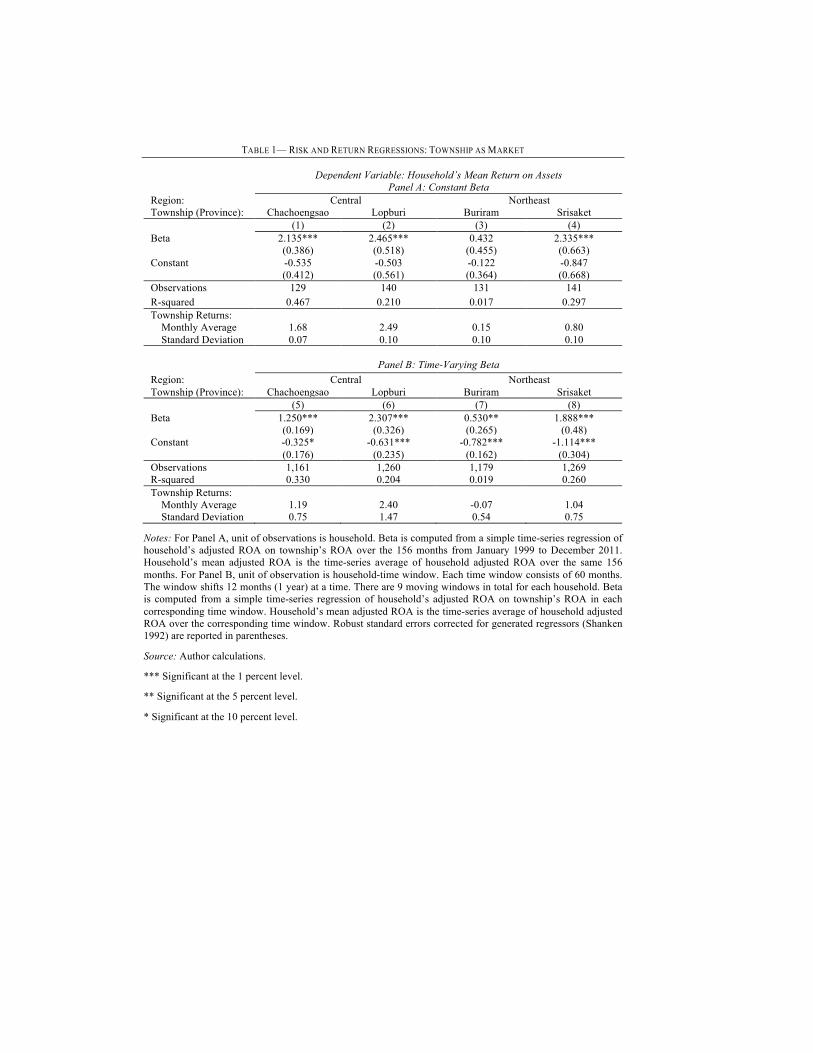
TABLE 1— RISK AND RETURN REGRESSIONS: TOWNSHIP AS MARKET

Dependent Variable: Household’s Mean Return on Assets Panel A: Constant Beta Region: Central Northeast Township (Province): Chachoengsao Lopburi Buriram Srisaket (1) (2) (3) (4) Beta 2.135*** 2.465*** 0.432 2.335*** (0.386) (0.518) (0.455) (0.663) Constant -0.535 -0.503 -0.122 -0.847 (0.412) (0.561) (0.364) (0.668) Observations 129 140 131 141 R-squared 0.467 0.210 0.017 0.297 Township Returns: Monthly Average 1.68 2.49 0.15 0.80 Standard Deviation 0.07 0.10 0.10 0.10 Panel B: Time-Varying Beta Region: Central Northeast Township (Province): Chachoengsao Lopburi Buriram Srisaket (5) (6) (7) (8) Beta 1.250*** 2.307*** 0.530** 1.888*** (0.169) (0.326) (0.265) (0.48) Constant -0.325* -0.631*** -0.782*** -1.114*** (0.176) (0.235) (0.162) (0.304) Observations 1,161 1,260 1,179 1,269 R-squared 0.330 0.204 0.019 0.260 Township Returns: Monthly Average 1.19 2.40 -0.07 1.04 Standard Deviation 0.75 1.47 0.54 0.75

Notes: For Panel A, unit of observations is household. Beta is computed from a simple time-series regression of household’s adjusted ROA on township’s ROA over the 156 months from January 1999 to December 2011. Household’s mean adjusted ROA is the time-series average of household adjusted ROA over the same 156 months. For Panel B, unit of observation is household-time window. Each time window consists of 60 months. The window shifts 12 months (1 year) at a time. There are 9 moving windows in total for each household. Beta is computed from a simple time-series regression of household’s adjusted ROA on township’s ROA in each corresponding time window. Household’s mean adjusted ROA is the time-series average of household adjusted ROA over the corresponding time window. Robust standard errors corrected for generated regressors (Shanken 1992) are reported in parentheses.

Source: Author calculations.

*** Significant at the 1 percent level.

** Significant at the 5 percent level.

* Significant at the 10 percent level.

TABLE 2— RISK AND RETURN REGRESSIONS WITH HUMAN CAPITAL AND TIME-VARYING STOCHASTIC DISCOUNT

FACTOR: TOWNSHIP AS MARKET

Dependent Variable: Household’s Mean Return on Assets Panel A: Human Capital

Region: Central Northeast Township (Province): Chachoengsao Lopburi Buriram Srisaket (1) (2) (3) (4) Beta with respect to 1.242*** 2.233*** 0.564*** 1.813*** return on market physical capital (ra) (0.163) (0.329) (0.271) (0.49) Beta with respect to 0.00177 0.0217 -0.0524 0.149 return on market human capital (rh) (0.056) (0.187) (0.181) (0.363) Constant -0.307* -0.584** -0.757*** -1.080*** (0.176) (0.232) (0.164) (0.310) Observations 1,161 1,260 1,179 1,269 R-squared 0.329 0.203 0.021 0.270 Panel B: Time-Varying Stochastic Discount Factor Region: Central Northeast Township (Province): Chachoengsao Lopburi Buriram Srisaket (5) (6) (7) (8) Beta with respect to 1.094*** 2.005*** 0.392 1.893*** return on market physical capital (ra) (0.148) (0.334) (0.242) (0.45) Beta with respect to -0.00542 0.0375 -0.0310 0.179 return on market human capital (rh) (0.061) (0.185) (0.171) (0.354) Beta with respect to -0.00441 0.00246 0.0333 0.0789 residual log consumption (cay) (0.055) (0.17) (0.149) (0.324) Beta with respect to -0.00533 -0.0304 -0.131 -0.101 the interaction cay*ra (0.065) (0.216) (0.168) (0.351) Beta with respect to 0.00134 -0.000574 0.0109 -0.0130 the interaction cay*rh (0.035) (0.162) (0.142) (0.315) Constant -0.156 -0.464** -0.589*** -1.164*** (0.178) (0.223) (0.162) (0.268) Observations 1,161 1,260 1,179 1,269 R-squared 0.315 0.203 0.049 0.306

Notes: Unit of observation is household-time window. For Panel A, beta’s are computed from a multivariate time-series regression of household’s monthly adjusted ROA on township’s monthly return on market physical capital (ra) and township’s return on human capital (ry), which is proxied by the monthly growth rate of township’s total labor income. Regressions are performed on moving windows of 60 months. The window then shifts 12 months (1 year) at a time and there are 9 moving windows in total for each household. Household’s mean adjusted ROA is the time-series average of household adjusted ROA over the corresponding time window. For Panel B, similar analysis is performed, with additional explanatory variables. Residual log consumption is the residual computed from time-series regression of township’s monthly log food consumption on township’s total physical asset at the beginning of the month and township’s total labor income during that month. Interaction terms are then defined accordingly. Robust standard errors corrected for generated regressors (Shanken 1992) are reported in parentheses.

Source: Author calculations.

*** Significant at the 1 percent level.

** Significant at the 5 percent level.

* Significant at the 10 percent level.

TABLE 3— CONTRIBUTION OF IDIOSYNCRATIC RISK TO TOTAL RISK AND TOTAL RISK PREMIUM (PERCENT)

Panel A: Baseline Specification Region: Central Township (Province): Chachoengsao Lopburi p25 p50 p75 p25 p50 p75 Contribution to Total Risk (Variance)

93.9 98.1 99.7 92.3 97.6 99.5

Contribution to Total Risk Premium

4.7 21.6 45.4 41.7 61.5 88.7

Percentage of Diversified Idiosyncratic Risk

98.6 99.6 100.0 92.4 96.3 99.9

Region: Northeast Township (Province): Buriram Srisaket p25 p50 p75 p25 p50 p75 Contribution to Total Risk (Variance)

84.0 94.0 98.2 43.8 65.9 88.9

Contribution to Total Risk Premium

105.6 118.7 152.8 13.3 28.8 53.9

Percentage of Diversified Idiosyncratic Risk

111.2 135.2 172.2 67.4 82.0 90.0

Panel B: Robustness Specification Region: Central Township (Province): Chachoengsao Lopburi p25 p50 p75 p25 p50 p75 Contribution to Total Risk (Variance)

77.4 84.9 89.0 80.2 88.0 91.6

Contribution to Total Risk Premium

6.3 32.6 56.6 21.2 54.9 102.2

Percentage of Diversified Idiosyncratic Risk

79.4 93.4 100.3 69.6 94.9 110.2

Region: Northeast Township (Province): Buriram Srisaket p25 p50 p75 p25 p50 p75 Contribution to Total Risk (Variance)

73.4 79.7 87.1 40.9 55.0 68.9

Contribution to Total Risk Premium

35.4 88.4 147.0 9.1 19.5 33.3

Percentage of Diversified Idiosyncratic Risk

75.5 112.7 153.6 63.4 79.9 89.4

Notes: Unit of observation is household. Panel A presents the results from a baseline specification, as shown in equation (4), using the empirical results from Columns (1)-(4) of Table 1. Panel B presents the results from a full robustness specification, as shown in equation (6), using the empirical results from Columns (5)-(8) of Table 2. The numbers for each household are the average across estimates from nine different time-shifting windows.

Source: Author calculations.

TABLE 4— AGGREGATE RISK, IDIOSYNCRATIC RISK, AND RATE OF RETURN: TOWNSHIP AS MARKET

Dependent Variable: Household’s Mean Return on Assets Panel A: Baseline Specification Region: Central Northeast Township (Province): Chachoengsao Lopburi Buriram Srisaket (1) (2) (3) (4) Beta with respect to return on 1.214*** 1.395*** -0.130 1.383*** market physical capital (ra) (0.266) (0.292) (0.359) (0.296) Sigma 0.00283*** 0.00407*** 0.00318*** 0.00425*** (0.000727) (0.000606) (0.00113) (0.000534) Constant -0.606 -1.525*** -0.644* -1.312** (0.393) (0.552) (0.368) (0.575) Observations 129 140 131 141 R-squared 0.536 0.297 0.120 0.513 Panel B: Robustness Specification Region: Central Northeast Township (Province): Chachoengsao Lopburi Buriram Srisaket (5) (6) (7) (8) Beta with respect to return on 0.487*** 1.105*** 0.0137 1.331*** market physical capital (ra) (0.194) (0.341) (0.248) (0.442) Beta with respect to return on 0.00598 0.06 -0.0411 0.0799 market human capital (rh) (0.054) (0.18) (0.168) (0.335) Beta with respect to -0.0117 -0.00401 0.0106 0.0376 residual log consumption (cay) (0.049) (0.168) (0.145) (0.321) Beta with respect to -0.0117 0.0245 -0.0686 -0.0560 the interaction cay*ra (0.056) (0.214) (0.162) (0.344) Beta with respect to -0.00166 -0.000644 0.00392 -0.0127 the interaction cay*rh (0.034) (0.162) (0.141) (0.314) Sigma 0.00428*** 0.00467*** 0.00389*** 0.00367*** (0.000689) (0.000400) (0.000435) (0.000296) Constant -0.489*** -1.535*** -1.356*** -1.491*** (0.171) (0.214) (0.151) (0.237) Observations 1,161 1,260 1,179 1,269 R-squared 0.433 0.330 0.196 0.446

Notes: Unit of observation is household-time window. For Panel A, beta’s are computed from a time-series regression of household’s monthly adjusted ROA on township’s monthly return on market physical capital (ra). For Panel B, beta’s are computed from a multivariate time-series regression of household’s monthly adjusted ROA on township’s monthly return on market physical capital (ra) and township’s return on human capital (rh), and township’s residual log consumption (cay). Township’s return on human capital (ry) is proxied by the monthly growth rate of township’s total labor income. Township’s residual log consumption is the residual computed from time-series regression of township’s monthly log food consumption on township’s total physical asset at the beginning of the month and township’s total labor income during that month. Interaction terms are then defined accordingly. Sigma is the variance of error terms from regressions used to estimate beta’s for each household-time window. Robust standard errors corrected for generated regressors are reported in parentheses.

Source: Author calculations.

*** Significant at the 1 percent level.

** Significant at the 5 percent level.

* Significant at the 10 percent level.

TABLE 5— IDIOSYNCRATIC INCOME, CONSUMPTION, GIFT, AND LENDING

Dependent Variable: Net Gift Outflow

Net Lending

Net Gift Outflow Plus Net Lending Consumption

Idiosyncratic Income 13.02*** 27.67*** 40.66*** 4.857** (4.795) (7.507) (9.000) (2.081) Province-Month Fixed Effects Yes Yes Yes Yes Household Fixed Effects Yes Yes Yes Yes Observations 81,664 81,712 81,664 81,712 R-squared 0.011 0.009 0.009 0.014 Number of Households 541 541 541 541

Notes: Unit of observation is household-month. Net gift outflow is defined as gift outflow minus gift inflow. Net lending is defined as lending minus borrowing. Robust standard errors are in parentheses.

Source: Author calculations.

*** Significant at the 1 percent level.

** Significant at the 5 percent level.

* Significant at the 10 percent level.

TABLE 6— DETERMINANTS OF RATE OF RETURNS AND RISKS

Region Central Northeast Province Chachoengsao Lopburi Buriram Srisaket Panel A: Simple Rate of Return Total Initial Wealth -0.0140** 0.534*** -0.594** -2.149*** (0.00694) (0.0791) (0.255) (0.323) Household Size -0.0868 -0.729*** -0.0651 -0.144 (0.177) (0.249) (0.169) (0.228) Age of Household Head -0.0417** 0.00155 0.00627 0.00231 (0.0201) (0.0211) (0.0142) (0.0209) Education of Household -0.115 -0.469*** 0.128 -0.492*** Head (0.136) (0.120) (0.0823) (0.133) Household Head 0.590 -0.597 -0.997** 1.710*** Gender (Male=1) (0.444) (0.510) (0.415) (0.510) Constant 4.434** 4.472** 0.101 4.636*** (1.815) (1.766) (1.103) (1.791) R-squared 0.014 0.078 0.022 0.084 Panel B: Risk-Adjusted Rate of Return Total Initial Wealth 0.0287*** 0.711*** -0.323 -0.109 (0.00806) (0.0691) (0.262) (0.192) Household Size 0.182 -0.872*** -0.239 -0.577*** (0.123) (0.205) (0.146) (0.166) Age of Household Head 0.0217 0.0338* 0.0257** 0.0550*** (0.0133) (0.0174) (0.0125) (0.0148) Education of Household 0.209* -0.368*** 0.0896 -0.252** Head (0.108) (0.106) (0.0746) (0.108) Household Head -1.580*** -0.291 -0.685* -0.0355 Gender (Male=1) (0.345) (0.369) (0.386) (0.401) Constant -2.320* -0.815 -1.911** -2.299* (1.204) (1.494) (0.964) (1.233) R-squared 0.026 0.128 0.027 0.080 Panel C: Aggregate Risk Total Initial Wealth -0.0261*** -0.00532 -0.178*** -0.831*** (0.00397) (0.0148) (0.0572) (0.0935) Household Size -0.141** 0.0543 0.0622 0.224*** (0.0695) (0.0491) (0.0444) (0.0526) Age of Household Head -0.0482*** -0.0152*** -0.00635 -0.0115** (0.0108) (0.00479) (0.00432) (0.00540) Education of Household -0.266*** -0.0172 0.000534 -0.111*** Head (0.0529) (0.0158) (0.0187) (0.0225) Household Head 1.766*** 0.0687 0.304*** 0.789*** Gender (Male=1) (0.212) (0.122) (0.0936) (0.117) Constant 4.888*** 1.574*** 0.847*** 2.326*** (0.918) (0.366) (0.313) (0.429) R-squared 0.080 0.164 0.043 0.169 Panel D: Idiosyncratic Risk Total Initial Wealth -6.902*** -34.73*** -68.39*** -239.2*** (1.087) (7.917) (17.98) (35.16) Household Size -51.43*** 23.16 43.24** 27.56 (19.67) (17.68) (18.51) (26.59) Age of Household Head -9.930*** -1.943 -4.848*** -9.827*** (2.391) (1.529) (1.549) (2.270) Education of Household -49.46*** -8.927 9.993 -21.49*

Head (10.47) (5.995) (6.210) (11.86) Household Head 319.9*** -109.6 -63.05 153.8*** Gender (Male=1) (48.73) (77.08) (46.39) (58.81) Constant 1,081*** 648.4*** 505.1*** 1,038*** (216.8) (141.2) (105.9) (190.6) R-squared 0.072 0.050 0.041 0.109 Observations 1,082 1,195 1,100 1,172

Notes: Unit of observation is household-round (shifting time window). For each household, beta and sigma are estimated from the regression in equation (6). Beta is the regression coefficient with respect to aggregate return on physical assets. Sigma is the variance of the error terms from the regression. Household size is the number of household members aged 15-64. Age of household head was as of the end of December 1998. Initial wealth is in million baht. All regressions include village fixed effects. Robust standard errors are reported in parentheses.

Source: Author calculations.

*** Significant at the 1 percent level.

** Significant at the 5 percent level.

* Significant at the 10 percent level.

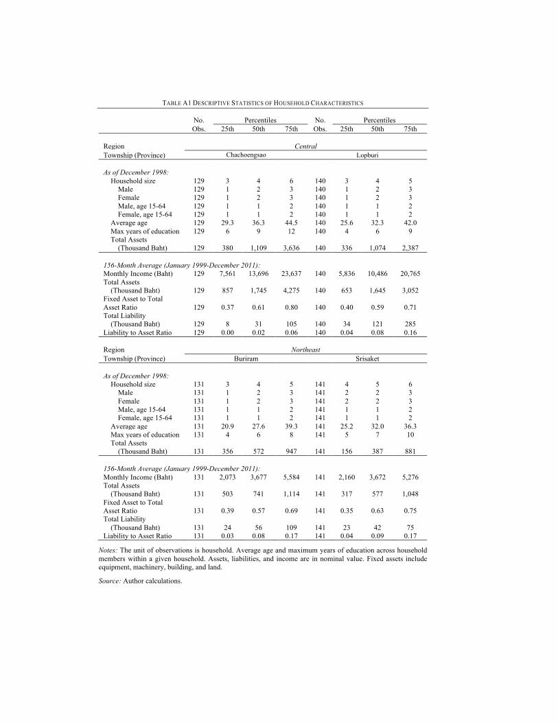
TABLE A1 DESCRIPTIVE STATISTICS OF HOUSEHOLD CHARACTERISTICS

No. Percentiles No. Percentiles Obs. 25th 50th 75th Obs. 25th 50th 75th

Region Central Township (Province) Chachoengsao Lopburi As of December 1998: Household size 129 3 4 6 140 3 4 5 Male 129 1 2 3 140 1 2 3 Female 129 1 2 3 140 1 2 3 Male, age 15-64 129 1 1 2 140 1 1 2 Female, age 15-64 129 1 1 2 140 1 1 2 Average age 129 29.3 36.3 44.5 140 25.6 32.3 42.0 Max years of education 129 6 9 12 140 4 6 9 Total Assets (Thousand Baht) 129 380 1,109 3,636 140 336 1,074 2,387 156-Month Average (January 1999-December 2011): Monthly Income (Baht) 129 7,561 13,696 23,637 140 5,836 10,486 20,765 Total Assets (Thousand Baht) 129 857 1,745 4,275 140 653 1,645 3,052 Fixed Asset to Total Asset Ratio 129 0.37 0.61 0.80 140 0.40 0.59 0.71 Total Liability (Thousand Baht) 129 8 31 105 140 34 121 285 Liability to Asset Ratio 129 0.00 0.02 0.06 140 0.04 0.08 0.16 Region Northeast Township (Province) Buriram Srisaket As of December 1998: Household size 131 3 4 5 141 4 5 6 Male 131 1 2 3 141 2 2 3 Female 131 1 2 3 141 2 2 3 Male, age 15-64 131 1 1 2 141 1 1 2 Female, age 15-64 131 1 1 2 141 1 1 2 Average age 131 20.9 27.6 39.3 141 25.2 32.0 36.3 Max years of education 131 4 6 8 141 5 7 10 Total Assets (Thousand Baht) 131 356 572 947 141 156 387 881 156-Month Average (January 1999-December 2011): Monthly Income (Baht) 131 2,073 3,677 5,584 141 2,160 3,672 5,276 Total Assets (Thousand Baht) 131 503 741 1,114 141 317 577 1,048 Fixed Asset to Total Asset Ratio 131 0.39 0.57 0.69 141 0.35 0.63 0.75 Total Liability (Thousand Baht) 131 24 56 109 141 23 42 75 Liability to Asset Ratio 131 0.03 0.08 0.17 141 0.04 0.09 0.17

Notes: The unit of observations is household. Average age and maximum years of education across household members within a given household. Assets, liabilities, and income are in nominal value. Fixed assets include equipment, machinery, building, and land.

Source: Author calculations.

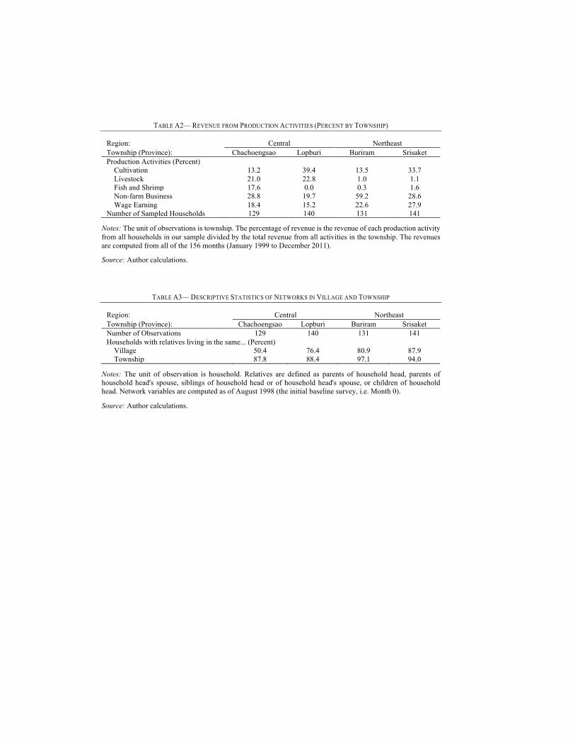
TABLE A2— REVENUE FROM PRODUCTION ACTIVITIES (PERCENT BY TOWNSHIP)

Region: Central Northeast Township (Province): Chachoengsao Lopburi Buriram Srisaket Production Activities (Percent) Cultivation 13.2 39.4 13.5 33.7 Livestock 21.0 22.8 1.0 1.1 Fish and Shrimp 17.6 0.0 0.3 1.6 Non-farm Business 28.8 19.7 59.2 28.6 Wage Earning 18.4 15.2 22.6 27.9 Number of Sampled Households 129 140 131 141

Notes: The unit of observations is township. The percentage of revenue is the revenue of each production activity from all households in our sample divided by the total revenue from all activities in the township. The revenues are computed from all of the 156 months (January 1999 to December 2011).

Source: Author calculations.

TABLE A3— DESCRIPTIVE STATISTICS OF NETWORKS IN VILLAGE AND TOWNSHIP

Region: Central Northeast Township (Province): Chachoengsao Lopburi Buriram Srisaket Number of Observations 129 140 131 141 Households with relatives living in the same... (Percent) Village 50.4 76.4 80.9 87.9 Township 87.8 88.4 97.1 94.0

Notes: The unit of observation is household. Relatives are defined as parents of household head, parents of household head's spouse, siblings of household head or of household head's spouse, or children of household head. Network variables are computed as of August 1998 (the initial baseline survey, i.e. Month 0).

Source: Author calculations.

TABLE A4— DESCRIPTIVE STATISTICS OF RETURN ON ASSETS: QUARTILES BY TOWNSHIP

No. Percentiles No. Percentiles Obs. 25th 50th 75th Obs. 25th 50th 75th Region: Central Province (Township): Chachoengsao Lopburi Mean 129 -1.72 0.38 3.99 140 -1.67 1.46 4.53 Standard Deviation 129 4.38 7.56 16.61 140 10.16 16.51 24.77 Coef. of Variation 129 2.02 3.14 5.46 140 3.27 4.65 8.85 Region: Northeast Province (Township): Buriram Srisaket Mean 131 -1.32 0.28 1.56 141 0.21 1.99 4.29 Standard Deviation 131 8.38 13.92 22.59 141 10.16 16.78 26.87 Coef. of Variation 131 4.03 8.70 17.48 141 4.03 5.92 11.52

Notes: Unit of observations is households. ROA is rate of return on household’s total asset, computed by household’s net income (net of compensation to household labor) divided by household’s average total assets over the month. ROA is real return, adjusted by regional Consumer Price Index from the Bank of Thailand, and reported in annualized percentage. Mean, standard deviation, and coefficient of variation of ROA are computed from monthly ROA for each household over 156 months (January 1999 to December 2011). The percentiles are across households in each township.

Source: Author calculations.

TABLE A5— RISK AND RETURN REGRESSIONS: VILLAGE AS MARKET

Dep. Var.: Household’s Mean ROA Region: Central Province: Chachoengsao Lopburi Village: 02 04 07 08 01 03 04 06 Beta 2.473*** 3.232*** 6.741*** 0.720 2.163 3.185 4.399*** 4.884***

(0.477) (0.595) (1.877) (0.894) (3.688) (2.746) (1.400) (1.493) Constant -1.105 -0.333 -0.739 1.162 -0.827 0.312 0.257 -1.629 (0.899) (0.756) (0.821) (0.984) (1.434) (0.873) (0.572) (1.503) No. Obs. 35 36 27 31 34 29 37 40 R-squared 0.449 0.702 0.446 0.036 0.012 0.126 0.472 0.337 Village Returns: Month Avg. 1.09 1.48 4.13 0.73 2.03 2.49 2.48 2.85 Std. Dev. 0.14 0.08 0.50 0.12 0.17 0.34 0.14 0.33 Region: Northeast Province: Buriram Srisaket Village: 02 10 13 14 01 06 09 10 Beta 0.827 0.547 0.217 0.697 2.759*** 3.680*** 1.557** 1.902*

(1.470) (1.566) (0.823) (1.298) (0.746) (2.015) (1.326) (1.101) Constant -0.628 0.346 0.684 -0.541 -2.407** -0.558 0.735 -1.748 (0.417) (1.197) (0.831) (0.688) (1.172) (1.661) (1.001) (1.907) No. Obs. 34 28 34 35 38 42 39 22 R-squared 0.022 0.010 0.003 0.014 0.510 0.387 0.114 0.149 Village Returns: Month Avg. -0.14 1.56 0.36 -0.52 -0.57 1.88 0.87 0.95 Std. Dev. 0.11 0.14 0.23 0.17 0.16 0.12 0.13 0.15

Notes: Unit of observations is household. Beta is computed from a simple time-series regression of household adjusted ROA on village ROA over the 156 months from January 1999 to December 2011. Household’s mean adjusted ROA is the time-series average of household adjusted ROA over the same 156 months. Standard errors corrected for generated regressors (Shanken 1992) are reported in parentheses.

*** Significant at the 1 percent level.

** Significant at the 5 percent level.

* Significant at the 10 percent level.

TABLE A6— RISK AND RETURN REGRESSIONS: NETWORK AS MARKET

Dependent Variable: Household’s Mean ROA Region: Central Province: Lopburi Village: 01 03 04 06 Network: 03 03 06 01 Beta -3.088 3.265 7.366*** 5.189*** (4.302) (4.033) (2.383) (0.881) Constant 0.433 1.523 0.123 -1.655 (1.448) (1.244) (0.865) (1.799) Observations 16 18 20 33 R-squared 0.012 0.041 0.464 0.345 Network Returns: Monthly Average 2.03 2.46 2.52 2.85 Standard Deviation 0.20 0.41 0.13 0.35 Region: Northeasst Province: Buriram Srisaket Village: 13 14 01 06 09 Network: 03 03 03 02 02 Beta 1.373 0.728 2.842*** 3.832** 1.540** (0.988) (1.046) (0.722) (1.484) (0.618) Constant -0.249 -0.460 -2.205* -0.452 0.554 (0.694) (0.794) (1.226) (1.845) (1.025) Observations 23 27 23 37 36 R-squared 0.184 0.015 0.365 0.374 0.134 Network Returns: Monthly Average 0.38 -0.52 -0.58 1.88 0.87 Standard Deviation 0.20 0.16 0.14 0.13 0.13

Notes: Unit of observations is household. Beta is computed from a simple time-series regression of household’s adjusted ROA on network’s ROA over the 156 months from January 1999 to December 2011. Household’s mean adjusted ROA is the time-series average of household adjusted ROA over the same 156 months. Standard errors corrected for generated regressors (Shanken 1992) are reported in parentheses.

*** Significant at the 1 percent level.

** Significant at the 5 percent level.

* Significant at the 10 percent level.

TABLE A7— DESCRIPTIVE STATISTICS OF HOUSEHOLD ALPHA: TOWNSHIP AS MARKET

Province No. Obs. Mean Std. Dev. Skewness Kurtosis Percentiles 25th 50th 75th Panel A: Return on Assets, Not Adjusted for Risks Central Chachoengsao 129 1.90 6.51 1.14 4.64 -1.72 0.38 3.99 Lopburi 140 1.37 6.31 -0.93 5.46 -1.67 1.46 3.16 Northeast Buriram 131 0.30 3.49 0.24 4.79 -1.32 0.28 1.39 Srisaket 141 2.83 5.87 0.75 5.53 0.21 1.99 4.29 Panel B: Return on Assets, Adjusted for Aggregate Risks Central Chachoengsao 129 0.68 5.52 0.44 5.17 -1.75 -0.15 2.59 Lopburi 140 0.28 5.81 -1.47 7.05 -1.98 1.00 3.16 Northeast Buriram 131 -0.28 3.60 -0.02 4.54 -1.94 -0.27 1.39 Srisaket 141 -0.11 4.84 0.24 5.76 -1.43 -0.08 1.18 Panel C: Return on Assets, Adjusted for Aggregate and Idiosyncratic Risks Central Chachoengsao 129 -0.49 4.52 -0.31 6.09 -2.21 -0.42 1.47 Lopburi 140 -1.54 5.27 -1.87 8.12 -3.49 -0.12 1.49 Northeast Buriram 131 -1.36 3.52 -0.73 4.38 -2.75 -0.75 0.54 Srisaket 141 -1.49 4.16 -0.68 5.70 -2.55 -0.72 0.31

Notes: Unit of observations is households. Panel A reports descriptive statistics of rate of return without adjusting for any risk (but adjusted for household’s own labor). Panel B report rate of return adjusted for aggregate risks, where risk premium is computed from market’s mean ROA (ra), market return on human capital (ry), residual consumption (cay), and their interactions cay*ra and cay*rh, as defined in equation (7) in the text. Panel C report rate of return adjusted for aggregate risks, where risk premium is computed from market’s mean ROA (ra), market return on human capital (ry), residual consumption (cay), and their interactions cay*ra and cay*rh, as well as idiosyncratic risk from sigma, as defined by equation (9b) in the text. For each household, the return in Panels B and C is averaged across 9 shifting time windows.

Source: Author calculations.