Risk Analysis of Development Programs A

P. P. PANDOLFINI

JOhNs hOPkINs APL TechNIcAL DIgesT, VOLume 27, Number 3 (2007)218

ARisk Analysis of Development Programs

Peter P. Pandolfini

set-theory methodology for risk analysis was first proposed by Benjamin Blanchard. The methodology is explained here

in terms of unfavorable events in technical, schedule, and cost performances. This is a comprehensive way to evaluate the risks contained in development programs from a program management perspective. By using program state tables and combining them with the assignment of Bayesian probabilities based on a maximum entropy principle, the overall risk of a program issue is evaluated using only the information at hand. The determination of iso-risk boundaries implied by this methodology is illustrated, and sample presentations of results are shown.

BASIC THEORYThe analysis of risk can be based on an adaptation of

a method introduced by Blanchard1 in the early 1980s that uses set theory to establish the probability of unfa-vorable events—the union of failures and impacts. In a program management environment, system develop-ment can be viewed in terms of favorable and unfa-vorable events, which contain all the events that can happen during program development (Fig. 1).

An event is the basic unit of the space. The sets con-sidered may contain technical, schedule, or cost perfor-mance events (or combinations thereof). Only the unfa-vorable events (i.e., failures and impacts) are used for determining risk. A failure is an unfavorable event, and an impact is an unfavorable event that follows a failure;

an impact may also be a failure. The unfavorable events, comprising several sets, are contained in Fig. 1.

In this diagram, T, S, and C denote technical, sched-ule, and cost performance events, respectively. L is the set of failures that can contain these events. The sets IT, IS, and IC contain the (unfavorable) impact events. Figure 1 contains 13 regions in its union of unfavor-able events, as summarized in Table 1. For example, the intersection of the IT and IS sets contains those unfavor-able events that have technical and schedule impacts; at the intersection of all these sets are the events that are simultaneously technical, cost, and schedule failures.

Risk is defined as the probability of occurrence of the unfavorable events (i.e., the probability of the union of

rIsk ANALYsIs OF DeVeLOPmeNT PrOgrAms

JOhNs hOPkINs APL TechNIcAL DIgesT, VOLume 27, Number 3 (2007) 219

all sets containing unfavorable events). In terms of the notation for the failure and impact sets,

RISK = P(L ∪ IT ∪ IS ∪ IC) = P(L ∪ I) ,

where I = IT ∪ IS ∪ IC, P( ) is the probability of the argu-ments (in this case, the union of several sets), and “∪” is the symbol used to denote the union. Thus, L ∪ IT ∪ IS ∪ IC (or L ∪ I in the shorthand introduced) is a compound event comprising the union of the four sets

of unfavorable events. The probability of occurrence of this compound event is derived from set theory and is

RISK = P(L) + P(I) − P(I|L)P(L) ,

where P(I|L) denotes a conditional probability (i.e., the probability of I given that L has occurred). (A simi-lar expression can be derived with the analysis of the RISK complement, RISK = P(L)P(I), where P(L) is the probability of the complement of a failure (i.e., a suc-cess) equal to (1 – P(L)), and P(I) is the probability of the complement of unfavorable impacts (i.e., favorable impacts) equal to (1 – P(I)). Substitution of the comple-mentary relationships, noting RISK = 1 – RISK, yields RISK = P(L) 1 P(I) 2 P(I) P(L).)

In the above expression three probabilities—P(L), P(I), and P(I|L)—must be evaluated to determine the iso-risk curves. It can be shown that the assumption that a value of P(I) equal to the value of P(I|L) yields a conservative set of iso-risk lines that are compatible with program management control (otherwise, risks may be underestimated). A discussion of other assump-tions for determining P(I|L) is beyond the scope of this article but would yield some interesting insights into the way iso-risk boundaries have been arbitrarily drawn in other analyses.

EVALUATION PROCESSTo apply this basic approach to a development pro-

gram risk analysis, a statement of potential risk is ana-lyzed with respect to four state tables. These tables con-tain language suggesting the state of the program with respect to a given issue (the issue for which risk is being evaluated). The “likelihood” table permits evaluation of probability of the failure associated with the issue, and the other three tables evaluate the extent of the impact of the failure in the technical, schedule, and cost dimen-sions. Figure 2 illustrates the flow.

Figure 1. Event space for program development. All program events are contained within the box. The unfavorable events are represented in a Venn diagram.

Table 1. Descriptions of regions containing unfavorable events.

Region Description

1 Technical impact events

2 Schedule impact events

3 Cost impact events

4 Technical and schedule impact events

5 Schedule and cost impact events

6 Technical and cost impact events

7 Technical FAILURE events

8 Technical and schedule FAILURE events

9 Schedule FAILURE events

10 Technical and cost FAILURE events

11 Cost FAILURE events

12 Schedule and cost FAILURE events

13 Technical, schedule, and cost FAILURE events

Figure 2. Risk evaluation process flow.

P. P. PANDOLFINI


Considering the potential risk statement, the state of the program is chosen from a likelihood table that lists program states from best to worst. This state will result in the assignment of P(L). Next, the state of the program with respect to the conditional realization of the situa-tion contained in the risk statement is chosen for technical, schedule, and cost impact using the “impact” tables. These states will result in the assignments of P(IT | L), P(IS | L), and P(IC | L), which are then combined into P(I | L).

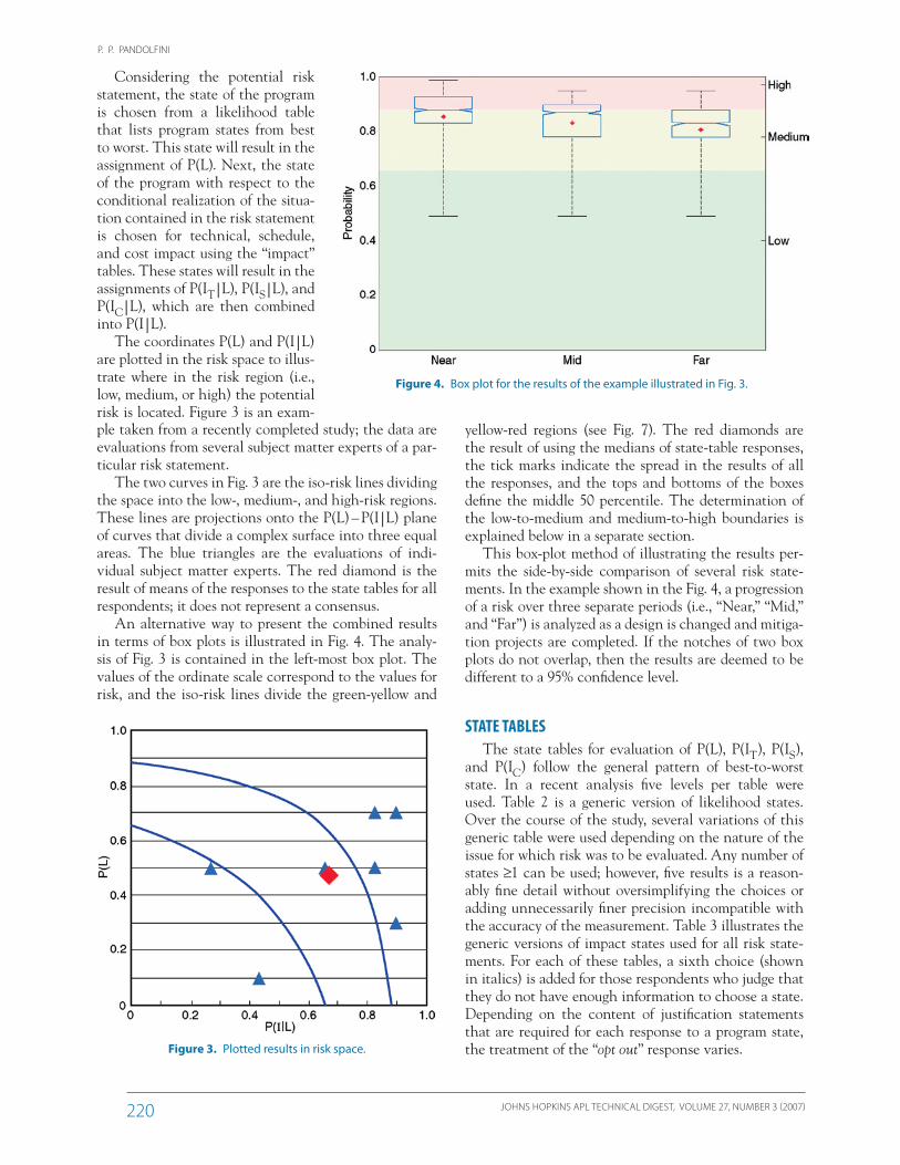
The coordinates P(L) and P(I | L) are plotted in the risk space to illus-trate where in the risk region (i.e., low, medium, or high) the potential risk is located. Figure 3 is an exam-

yellow-red regions (see Fig. 7). The red diamonds are the result of using the medians of state-table responses, the tick marks indicate the spread in the results of all the responses, and the tops and bottoms of the boxes define the middle 50 percentile. The determination of the low-to-medium and medium-to-high boundaries is explained below in a separate section.

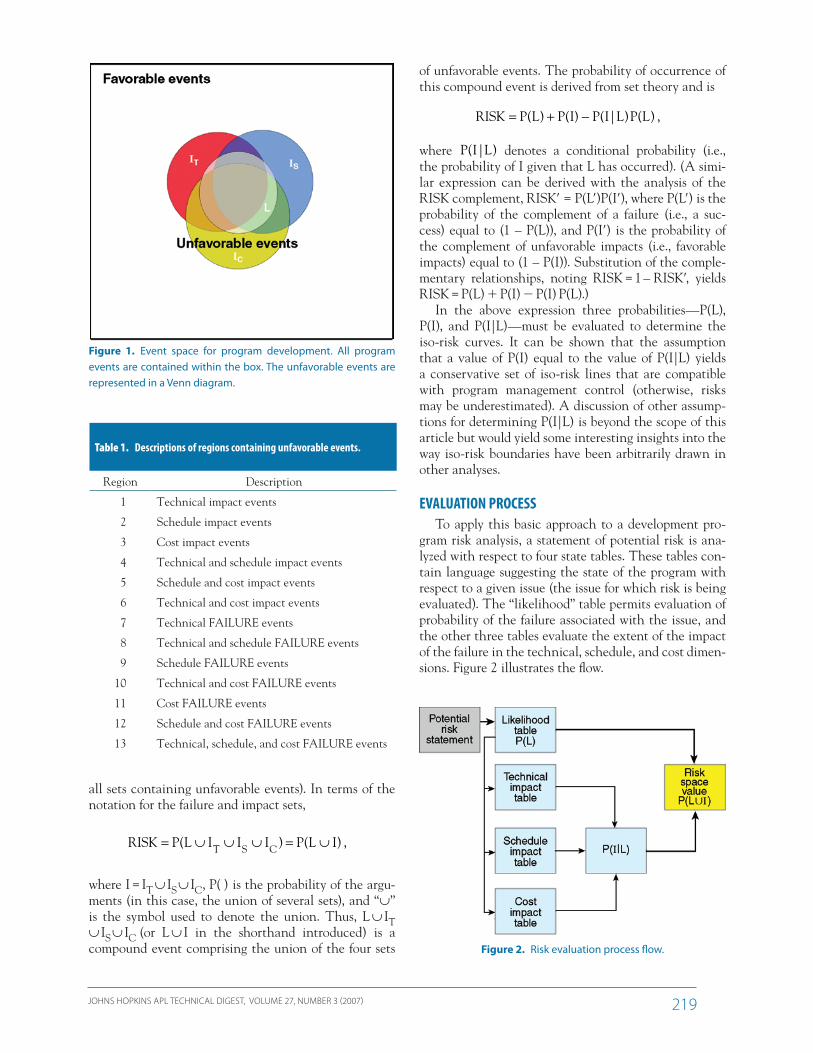
This box-plot method of illustrating the results per-mits the side-by-side comparison of several risk state-ments. In the example shown in the Fig. 4, a progression of a risk over three separate periods (i.e., “Near,” “Mid,” and “Far”) is analyzed as a design is changed and mitiga-tion projects are completed. If the notches of two box plots do not overlap, then the results are deemed to be different to a 95% confidence level.

STATE TABLESThe state tables for evaluation of P(L), P(IT), P(IS),

and P(IC) follow the general pattern of best-to-worst state. In a recent analysis five levels per table were used. Table 2 is a generic version of likelihood states. Over the course of the study, several variations of this generic table were used depending on the nature of the issue for which risk was to be evaluated. Any number of states ≥1 can be used; however, five results is a reason-ably fine detail without oversimplifying the choices or adding unnecessarily finer precision incompatible with the accuracy of the measurement. Table 3 illustrates the generic versions of impact states used for all risk state-ments. For each of these tables, a sixth choice (shown in italics) is added for those respondents who judge that they do not have enough information to choose a state. Depending on the content of justification statements that are required for each response to a program state, the treatment of the “opt out” response varies.Figure 3. Plotted results in risk space.

Figure 4. Box plot for the results of the example illustrated in Fig. 3.

ple taken from a recently completed study; the data are evaluations from several subject matter experts of a par-ticular risk statement.

The two curves in Fig. 3 are the iso-risk lines dividing the space into the low-, medium-, and high-risk regions. These lines are projections onto the P(L) – P(I | L) plane of curves that divide a complex surface into three equal areas. The blue triangles are the evaluations of indi-vidual subject matter experts. The red diamond is the result of means of the responses to the state tables for all respondents; it does not represent a consensus.

An alternative way to present the combined results in terms of box plots is illustrated in Fig. 4. The analy-sis of Fig. 3 is contained in the left-most box plot. The values of the ordinate scale correspond to the values for risk, and the iso-risk lines divide the green-yellow and



ASSIGNMENT OF PROBABILITY VALUES

A respondent (i.e., a subject matter expert) is asked to choose the state of the program with respect to the risk statement, but not assign a value to the probability that the program will experience the failure or impact. The assignment of prob-abilities to each state is developed by applying the maximum entropy principle.2

The probability of any event occurring in a given state is con-strained by 0 < P < 1 (note that the end values indicating certainty, 0 and 1, are not included in this range). For determining a value for P(L), given a state, it is asserted that the probability of a given fail-ure happening is such that P(L)A < P(L)B < P(L)C < P(L)D < P(L)E. Con-sider Fig. 5: the worse the state, the greater the probability of failure. That is the extent of our prior infor-mation with respect to the probabil-ities of failure assigned to the states. (If additional information is known, e.g., the specific probability of a par-ticular state, then it is incorporated directly into the state tables. The remaining unknown probabilities are determined by using the maxi-mum information entropy method.) Assigning the intervals between the discrete probabilities requires another constraint. This results in P(L)A = 0.1, P(L)B = 0.3, P(L)C = 0.5, P(L)D = 0.7, and P(L)E = 0.9.

This is how we arrive at these values: Referring to Fig. 5,

the sizes of the intervals (a, b, c, d, and e) dividing up the probabil-ity interval (0 to 1) can take on many different values and still satisfy P(L)A < P(L)B < P(L)C < P(L)D < P(L)E. However, if the additional maxi-mum information entropy constraint is imposed, then the quantity [ 2 a(log2a) 2 b(log2b) 2 c(log2c) 2 d(log2d) 2 e(log2e)] must be maximized. The maximum information entropy occurs when a = b = c = d = e = 0.2. Thus, P(L)A is greater than 0 and less than or equal to 0.2, and is set equal to 0.1, the mid-point of the interval. Similarly, the other probabilities P(L)B, P(L)C, P(L)D, and P(L)E are set to 0.3, 0.5, 0.7, and 0.9, respectively. A similar argu-ment is made for P(Ix | L)A, P(Ix | L)B, P(Ix | L)C, P(Ix | L)D, and P(Ix | L)E, where x = T, S, or C, to establish these values as 0.1, 0.3, 0.5, 0.7, and 0.9, respectively.

The two equations required to evaluate RISK,

RISK = P(L ∪ I) = P(L) + P(I) − P(I|L) P(L)

and

P(I|L) = P(IT|L ∪ IS|L ∪ IC|L)

= P(IT|L) + P(IS|L) + P(IC|L) − P(IS|IT ,L)P(IT|L)

− P(IC|IT ,L)P(IT|L) − P(IC|IS,L)P(IS|L)

+ P(IT|L)P(IS|L)P(IC|L) ,

contain eight independent probabilities: P(L), P(I), P(IT | L), P(IS | L), P(IC | L), P(IS | IT,L), P(IC | IT,L), and P(IC | IS, L). During a survey, four probabilities are measured, viz., P(L), P(IT | L), P(IS | L), and P(IC | L). For purposes of a practical evaluation, the values of P(IS | IT,L), P(IC | IT,L), and P(IC | IS,L) are assumed to be equal to P(IS | L), P(IC | L), and P(IC | L), respectively. This assumption simplifies the second equation; sample mea-surements from a completed study showed no significant differences from the P(IT | L), P(IS | L), and P(IC | L) measurements. The additional assumption that the value of P(I) is equal to P(I | L), as previously discussed, adds an additional level of conservatism in drawing the iso-risk boundaries.

The protocol of assigning a risk value for opt out responses is to rely on the maximum entropy principle. Usually, a value of 0.5 is used if the respondent indicates an unbiased ignorance of the state. If a collection of responses is being combined, the opt out response is usually not included because there are other responses to process, unless all the responses are opt out.

Table 2. Program likelihood states.

L Program state

A Best

B Good

C Average

D Fair

E Worst

F Opt out

Table 3. Program impact states.

IT, L IS, L IC, L Program state

F1 G1 H1 Little impact

F2 G2 H2 Low impact

F3 G3 H3 Moderate impact

F4 G4 H4 Large impact

F5 G5 H5 Very significant impact

F6 G6 H6 Opt out

P. P. PANDOLFINI


Figure 5. Division of the probability space.

ISO-RISK BOUNDARIESThe equation RISK = P(L) 1 P(I) 2 P(I | L)P(L), with

its simplifying assumption P(I) = P(I | L), yields the com-plex surface illustrated in Fig. 6. An iso-risk is defined as the locus of points on this surface where RISK is constant.

To establish the classification boundaries among, say, low, medium, and high risks, the iso-risk curves that divide the three-dimensional surface area into equal parts must be found. The analysis was conducted using Mathematica, and the result is that R = 0.657917 and 0.880472 divides the surface bounded by 0 < P,C < 1 into thirds. The projection of these boundaries onto the P-C plane (corresponding to the P(L) 2 P(I | L) plane in the current analysis) is shown in Fig. 7. Figure 7 represents a projection of the three-dimensional surface onto a plane yielding a “distorted” look to the low-medium-high risk areas when they are viewed in two dimensions and is analogous to Fig. 3, showing the source of the iso-risk boundaries. The shape of these iso-risk boundaries depends on the relationship between P(I | L) and P(I)—assumed to have equal values in the current analysis. Distortion of these boundaries by other assumptions is a subject for a separate paper.

Figure 6. Risk surface for R = P 1 C 2 P*C. Figure 7. Projection of iso-risk boundaries.

RISK PHASE SPACEAs a result of the foregoing anal-

ysis, a large but finite phase space for the discrete values of RISK is estab-lished. For the risk equation and its simplifying assumptions that reduce its evaluation to four probability measurements (i.e., P(L), P(IT | L), P(IS | L), and P(IC | L)), and the five

values (i.e., 0.1, 0.3, 0.5, 0.7, and 0.9) per the maximum information entropy argument, to which they are lim-ited, there are 625 ways to compute a RISK value (54). However, many of these values occupy the same phase (i.e., equal values of RISK, although the location may be different in the plane); there are only 55 discrete phases, 4 of which fall into the “green” region (7.3%), 12 into the “yellow” region (21.8%), and 39 into the “red” region (70.9%).

As part of an analysis, the distribution of the risk levels may be compared to the distribution of levels in the phase space (by, for example, employing a chi-squared test on the distribution of green-yellow-red results). Such an analysis may provide insight into whether the results are random or a consequence of deliberation by subject matter experts.

CONCLUDING REMARKSThis article presents a derivation of the methodology

first introduced by Blanchard and combines his approach with a way of assigning probabilities that are determined by a maximum entropy constraint. In this approach, program issues are analyzed using state tables. Both fail-ures and impacts are treated as unfavorable events and



Peter P. Pandolfini

The AuthorPeter P. Pandolfini is a member of APL’s Principal Professional Staff. He graduated from the City College of New York (CCNY) with a civil engineering degree and from Rutgers University with M.S. and Ph.D. degrees in mechanical engineering. In 1984,

he was a member of the first technical management class to graduate from the JHU G. W. C. Whiting School evening program. As a 35-year member of the APL staff, Dr. Pandolfini has performed research on air-breathing engines and on alternate energy conversion power systems. During the 1990s, he led APL’s participation in several aircraft development programs. Currently, he is a member of the National Security Analysis Department and leads a section that specializes in modeling and simulation assess-ment, including tasks for the Assessment Division of the Navy. Dr. Pandolfini is a Registered Profes-sional Engineer in Maryland. His e-mail address is [email protected].

are linked in their union. The assigned probabilities to failures and impacts are used in the risk equation, which computes the probability of the union of unfavorable events. The use of the probability of the union ensures that program risks are not underestimated.

The separation of the levels of risk (into, e.g., three categories—low, medium, or high) is accomplished by dividing the area of the complex sur-face generated by the risk equation and projecting the divisions, the iso-risks, onto a plane.

The use of set theory and the maximum entropy principle leads to a straightforward and elegant way to analyze program risks on a sound math-ematical basis. This method, with the judicious use of state tables, analyzes a program issue comprehensively in its technical, schedule, and cost perfor-mances—the types of events of interest in the management of development programs.

ACKNOWLEDGMENTS. The author wishes to thank eric greenberg and Jack calman for their assistance in preparing several illustrations. eric’s analysis supplied the box plot illustrated in Fig. 4, and Jack’s analysis prepared Fig. 6.

REFERENCES AND NOTES

1Blanchard, B. S., System Engineering Management, 3rd Ed., John Wiley & Sons, Inc., Hoboken, NJ (2004).

2Jaynes, E. T., Probability Theory, The Logic of Science, Cambridge University Press, Cambridge, UK (2004). See, especially, Chap. 11, which discusses the assignment of discrete prior prob-abilities and application of the entropy principle (i.e., application of Shannon’s information entropy). Jaynes published many other works employing this principle, but this text summarizes his lifework in this field.

Documents

Risk Analysis of Development Programs A