Business Risk Management Programs and Risk-balancing

Business Risk Management Programs and Risk-balancing Behavior in Ontario Hog Sector

by

Truc Thach Phan

A Thesis

presented to

The University of Guelph

In partial fulfilment of requirements for the degree of

Master of Science

in

Food, Agricultural and Resource Economics

Guelph, Ontario, Canada

© Truc Thach Phan, August 2018

ABSTRACT

BUSINESS RISK MANAGEMENT PROGRAMS AND RISK-BALANCING BEHAVIOR

IN ONTARIO HOG SECTOR

Truc Thach Phan

University of Guelph, 2018

Advisor:

Rakhal Sarker

Agri-food sectors in Canada are supported through safety net programs. CAIS/BRM

programs were designed to help producers reduce BR by mitigating negative income

shocks and reducing income variability. Nevertheless, according to the risk-balancing

hypothesis, farms may take more FR in response to a reduction in BR as a result of

program payments. If we find evidence of such behavior, risk-reduction efforts of

CAIS/BRM programs may not generate intended outcomes. This thesis employs OFID

tax-filing data over the 2003-2014 period to estimate the extent of risk-balancing in the

Ontario hog sector as a result of AgriStability payments under CAIS/BRM. We find that

that AgriStability payments were effective in reducing BR for medium and large farms but

not small farms. Controlling for other determinants of financial risk, our log-log fixed-

effects regression provides evidence of risk-balancing for medium and large farms in

Ontario hog sector.

iii

ACKNOWLEDGEMENTS

Thank you to my supervisor Dr. Rakhal Sarker for your guidance and support

throughout the entire research process, and to my Advisory Committee members, Dr.

Alfons Weersink and Dr.Yuna Lee, for your invaluable feedback and encouragement,

especially towards the final stage of my research. I would also like to extend my sincere

thanks to Dr. Getu Hailu for your constant encouragement, advice and support in all

your capacity, and Dr. Michael Von Massow for your interest and input into my project.

To all the professors in the department whose courses I attended, thank you for your

teaching and mentorship, which was beyond my expectation.

I feel thankful for all the spiritual encouragement from all of my friends at the

Vietnamese Christian Community in this city. And thank you Yong Liu and Yuetian for

your great help in getting me familiar with R software. This thesis could not have been

done without your extensive help and support. Also, thank you to Kathryn, Debbie and

Pat for all you have done for us behind the scene.

Thank you to my family, near and far, for your eternal love, confidence and great

support to me during my learning process as a student. My special thanks go to my

great Mom for the infinite love, who moved across the world to support me in the pursuit

of this degree. Finally, I would like to thank my partner, Ian Timperley, and my daughter,

Khue Nguyen, for their constant love, patience and endurance when I was a fireball of

stress that would explode at anytime during the tough time working on the thesis. For

you, I am forever grateful.

iv

TABLE OF CONTENTS

Abstract ............................................................................................................................ii

Acknowledgements ......................................................................................................... iii

Table of Contents ............................................................................................................iv

List of Tables .................................................................................................................. vii

List of Figures ................................................................................................................ viii

List of Abbreviations ........................................................................................................ x

List of Appendices ...........................................................................................................xi

1 CHAPTER 1: INTRODUCTION................................................................................ 1

1.1 Background ........................................................................................................ 1

1.1.1 Agriculture: an industry characterized by growing uncertainty and volatility 1

1.1.2 The Canadian Farm Business Risk Management programs ....................... 3

1.1.3 Risk-balancing behavior in Canadian farming industry: an overview ........... 6

1.2 Economic problem, economic research problem and motivation for the study... 9

1.2.1 Economic problem ....................................................................................... 9

1.2.2 Economic research problem ...................................................................... 10

1.2.3 Motivation for the study: why Ontario hog sector? ..................................... 11

1.3 Purpose and objectives .................................................................................... 16

1.4 Chapter outlines ............................................................................................... 16

2 CHAPTER 2. AN OVERVIEW OF CANADIAN FARM SAFETY-NET PROGRAMS AND ONTARIO HOG SECTOR .................................................................................... 18

2.1 Chapter introduction ......................................................................................... 18

2.2 Historical overview of farm safety net programs in Canada ............................. 18

v

2.3 BRM program under Growing Forward II (2013-2017) ..................................... 25

2.4 Crop Insurance Program .................................................................................. 27

2.5 Concluding remarks on the evolution of safety-net programs in Canada ......... 28

2.6 Ontario hog sector at a glance ......................................................................... 29

3 CHAPTER 3: LITERATURE REVIEW .................................................................... 35


3.2 The concept of business risk (BR) and financial risk (FR) ................................ 35

3.3 Review of recent studies related to the research questions ............................. 36

3.3.1 The extent of risk-balancing behavior ........................................................ 36

3.3.2 The effectiveness of BRM program – How to measure business risk? ...... 38

3.3.3 Crop Insurance and risk-balancing behavior ............................................. 40

3.4 Chapter summary ............................................................................................. 43

4 CHAPTER 4: ANALYTICAL FRAMEWORK........................................................... 49


4.2 Theoretical literature of risk-balancing ............................................................. 49

4.3 Collins (1985) with Crop Insurance purchase ................................................... 61

4.4 Chapter summary ............................................................................................. 66

5 Chapter 5: DATA, VARIABLE MEASURES AND DESCRIPTIVE STATISTICS .... 68


5.2 Data and variable definition .............................................................................. 68

5.2.1 Data sources and features ......................................................................... 68

5.2.2 Variable definition and empirical measurement ......................................... 69

5.3 Descriptive statistics and risk measurements ................................................... 73

5.3.1 Outlier detection – the distribution of Net Operating Income (NOI) ............ 73

vi

5.3.2 Descriptive statistics of key variables ........................................................ 76

5.3.3 Risk measurements ................................................................................... 81

5.4 Chapter summary ............................................................................................. 86

6 CHAPTER 6: RESEARCH METHODS AND EMPIRICAL RESULTS .................... 87


6.2 Empirical approaches ....................................................................................... 87

6.2.1 Effectiveness of CAIS/AgriStability payments ............................................ 87

6.2.2 Extent of risk-balancing ............................................................................. 87

6.3 Empirical results and discussion ...................................................................... 92

6.3.1 The risk-reducing effects of CAIS/AgriStability .......................................... 92

6.3.2 The extent of risk-balancing ....................................................................... 93

6.4 Chapter summary ........................................................................................... 104

7 CHAPTER 7: CONCLUSION ............................................................................... 105

7.1 Research summary ........................................................................................ 105

7.2 Policy implications .......................................................................................... 107

7.3 Contributions of the study............................................................................... 108

7.4 Suggestions for further research .................................................................... 108

References .................................................................................................................. 110

Appendices ................................................................................................................. 113

vii

LIST OF TABLES

Table 1. Top commodities in terms of market receipts ($ million) ................................. 31

Table 2. A synoptic review of empirical studies ............................................................. 44

Table 3. Summary of risk variables from Gabriel & Baker (1980), Collins (1985) and this study .............................................................................................................................. 67

Table 4. Variable summary ........................................................................................... 71

Table 5. Quartile statistics of NOI - After program payments ........................................ 75

Table 6. Results of Shapiro-Wilk normality test of NOI across farm size categories .... 76

Table 7. Descriptive statistics for key variables ............................................................. 77

Table 8. Descriptive Statistics by farm size categories.................................................. 79

Table 9. Risk-reducing effects of CAIS/ BRM - Business Risk ...................................... 93

Table 10. The extent of risk-balancing across farm size category – Pearson correlation coefficient ...................................................................................................................... 95

Table 11. First and second – order autocorrelation of residuals – OLS linear regressions ...................................................................................................................................... 96

Table 12. Attempted regressions................................................................................... 97

Table 13. Testing of cross-sectional dependence, autocorrelation and heteroscedasticity ...................................................................................................................................... 98

Table 14. Estimation results: fixed-effects log-log regression for whole sample ......... 100

Table 15. Estimation results: log-log regression by farm size categories .................... 103

viii

LIST OF FIGURES

Figure 1. Net farm income - aggregate across all farms, Canada, 1980 - 2016 .............. 2

Figure 2. Net farm income - aggregate across all farms, Ontario - 1980 - 2016 .............. 3

Figure 3. Layering and cost sharing of AgriStability payment under CAIS ...................... 5

Figure 4. Layering and cost sharing of AgriStability - Growing Forward I (2007 - 2012) . 6

Figure 5. Layering and cost sharing of AgriStability - Growing Forward II (2013 - 2018) 6

Figure 6. The effects of risk-reducing policies on farm's production ................................ 7

Figure 7. Total farm cash receipts by province .............................................................. 12

Figure 8. Provincial distribution of farm cash receipt in Canada – 2014 ........................ 12

Figure 9. Total farm cash receipts of Ontario 2003 – 2014 ........................................... 13

Figure 10. Provincial distribution of agricultural operations by farm numbers, 2006...... 13

Figure 11. Provincial distribution of agricultural operations by farm numbers, 2016...... 14

Figure 12. Net farm income in Ontario 2003 – 2014...................................................... 15

Figure 13. Direct net government payment by province, annual ($’000) ....................... 15

Figure 14. Canadian Risk Management programs: frequency and type of events covered ......................................................................................................................... 24

Figure 15. Hog numbers by province from census 2001 to 2016 (x1,000) .................... 29

Figure 16. Hog farms by province - Census 2001 to 2016 ............................................ 30

Figure 17. Percentage of Ontario hog number to Canada - Census 2001 to 2016 ....... 30

Figure 18. Number of hogs and hog farms in Ontario ................................................... 32

Figure 19. Ontario weekly hog price .............................................................................. 33

Figure 20. Ontario price for index 100 hogs live weight (1992-2017) ............................ 33

Figure 21. Ontario annual average 100% formula hog price (Can$/100kg) .................. 34

Figure 22. Gross and net returns/ hog in Ontario .......................................................... 34

ix

Figure 23. Density plot and boxplots of NOI across farm size categories ..................... 73

Figure 24. Box plot and density plot of NOI – Large size group (after outlier removal) . 74

Figure 25. Density plot of NOI across 3 size categories (after outlier removal) ............. 74

Figure 26. Sample distribution by farm size categories ................................................. 80

Figure 27. Average total risks by farm size categories- CV measure ............................ 81

Figure 28. Average BR by farm size categories- CV measure ...................................... 82

Figure 29. Average FR by farm size categories - CV measure ..................................... 83

Figure 30. Average FR by farm size categories – magnitude measure ......................... 84

Figure 31. Average BR of Medium farm size category– Skewness measure ................ 85

x

LIST OF ABBREVIATIONS

APF: Agricultural Policy Framework

BR: Business Risk

BRM: Business Risk Management

CAIS: Canadian Agricultural Income Stabilization

CI: Crop Insurance

CV: Coefficient of Variation

FCC: Farm Credit Canada

FR: Financial Risk

GFI: Growing Forward I

GFII: Growing Forward II

MAD: Median Absolute Deviation

NOI: Net Operating Income

OMAFRA: Ontario Ministry of Agriculture, Food and Rural Affairs

TR: Total Risk

VIF: Variance Inflation Factor

xi

LIST OF APPENDICES

Appendix 1. First-order condition of the expected utility function ................................ 113

Appendix 2. Second-order condition of the expected utility function ........................... 114

Appendix 3. T-test results for the risk-reducing effects of CAIS/ BRM on total risk .... 115

Appendix 4. Result of F- test for individual effects ...................................................... 116

Appendix 5. Results of Hausman test (robust) ............................................................ 117

Appendix 6. Variance Inflation Factor of explanatory variables ................................... 118

Appendix 7. Correlation matrix of explanatory variables ............................................. 119

Appendix 8. Estimation results: linear regressions by farm size categories ................ 120

1

1 CHAPTER 1: INTRODUCTION

1.1 Background

1.1.1 Agriculture: an industry characterized by growing uncertainty and volatility

The biological basis of agricultural production makes farms prone to uncertainty

with respect to yield. All farms are exposed to production risks, regardless of their sizes.

Yield loss of field crop farms may come from natural hazards and/ or the prevalence of

insects and diseases. For livestock farms, however, losses caused by infectious

diseases or adverse weather conditions are not uncommon. More importantly, losses

from a contagious disease outbreak may strike a myriad of farms, large or small, and hit

production of the entire sector very hard.

Changes in global climate may induce additional variability to farm production

and farm income. Due to climate change, rainfall could become more erratic in terms of

volume and timing and temperatures could swing wildly. Both changes may lead to

more frequent weather calamities like severe storms, flash flooding and droughts. Due

to these conditions, agricultural production could become seriously affected.

Closely associated with production uncertainty is the risk of price fluctuations.

Price uncertainty has long been a major issue in farming because expected prices could

vastly differ from actual prices due to the time gap between the decision to produce and

the realization of final production. Farm commodity prices have fluctuated dramatically

in recent years. For example, global price of corn experienced large swings in recent

years, which influenced not only the corn sector but also adversely impacted poultry,

beef and hog sectors. In particular, corn prices doubled from around $2 per bushel in

2006 to about $4 per bushel in 2007 and surged to $8 per bushel in the summer of

2012. Corn prices have since fallen back to $4 per bushel.

2

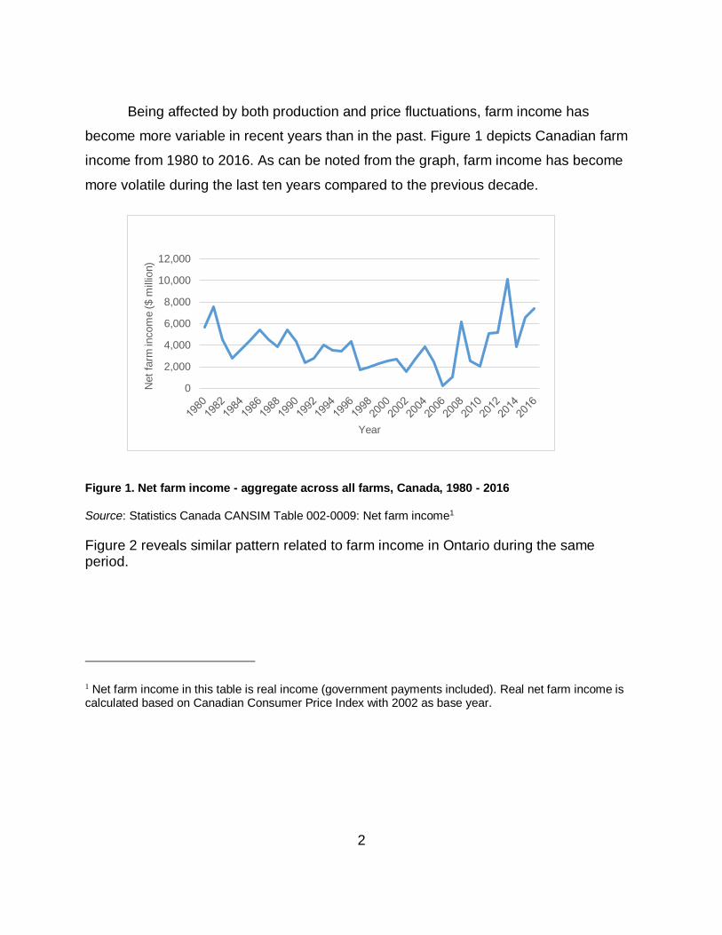
Being affected by both production and price fluctuations, farm income has

become more variable in recent years than in the past. Figure 1 depicts Canadian farm

income from 1980 to 2016. As can be noted from the graph, farm income has become

more volatile during the last ten years compared to the previous decade.

Figure 1. Net farm income - aggregate across all farms, Canada, 1980 - 2016

Source: Statistics Canada CANSIM Table 002-0009: Net farm income1

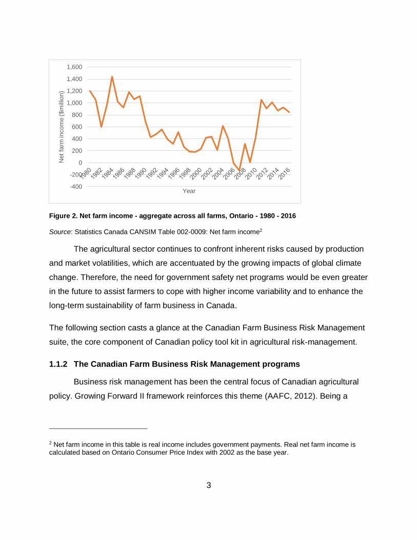
Figure 2 reveals similar pattern related to farm income in Ontario during the same period.

1 Net farm income in this table is real income (government payments included). Real net farm income is calculated based on Canadian Consumer Price Index with 2002 as base year.

0

2,000

4,000

6,000

8,000

10,000

12,000

Net

farm

incom

e ($ m

illio

n)

Year

3

Figure 2. Net farm income - aggregate across all farms, Ontario - 1980 - 2016

Source: Statistics Canada CANSIM Table 002-0009: Net farm income2

The agricultural sector continues to confront inherent risks caused by production

and market volatilities, which are accentuated by the growing impacts of global climate

change. Therefore, the need for government safety net programs would be even greater

in the future to assist farmers to cope with higher income variability and to enhance the

long-term sustainability of farm business in Canada.

The following section casts a glance at the Canadian Farm Business Risk Management

suite, the core component of Canadian policy tool kit in agricultural risk-management.

1.1.2 The Canadian Farm Business Risk Management programs

Business risk management has been the central focus of Canadian agricultural

policy. Growing Forward II framework reinforces this theme (AAFC, 2012). Being a

2 Net farm income in this table is real income includes government payments. Real net farm income is calculated based on Ontario Consumer Price Index with 2002 as the base year.

-400

-200

0

200

400

600

800

1,000

1,200

1,400

1,600N

et

farm

incom

e ($m

illio

n)

Year

4

whole farm-based income stabilization policy, the Canadian Farm Business Risk

Management (BRM) pillar target risks of all sizes and types of farms in Canada.

Under the current Growing Forward (hereinafter referred to as GF) (2013-2018),

AgriStability payment is triggered when the Program Year Margin falls below 70 percent

of the Reference Margin. Calculation of the Reference Margin for a given year is based

on an Olympic average3 of the preceding five years’ production margins. Starting in the

2013 Program Year, AgriStability payment will be calculated based on the Reference

Margin or the average Allowable Expenses in the years used to calculate the RM,

whichever is less (AAFC, 2011). For instance, if Reference Margin is $80,000 and the

average Allowable Expenses is $50,000, Reference Margin limit of $50,000 is applied to

calculate program payment. Besides, Reference Margin is also adjusted in order to

reflect any structural change that occurred on the farms. For instance, changing of

commodities, up or downsizing of farming operations. In these cases, historical margins

are adjusted, and Reference Margin is re-calculated using these adjusted figures. In

addition to this Tier of payment, Negative Margin is covered by the government at 70

percent of the portion of margin decline that is below zero, provided it does not exceed

the maximum program payment of $3 million per farm.

When the Program Year Margin loss is less than 30 percent of the Reference

Margin, farm operators are expected to manage such margin loss through a self-

managed producer – government saving account supported by AgriInvest. This is a

savings account built upon annual deposits based on a percentage of farms’ Allowable

Net Sales with matching contributions from federal, provincial, and territorial

governments. Farm operators can deposit up to 100 percent of their Allowable Net

Sales annually and receive matching government contribution on 1 percent of ANS.

Matching government contributions is capped at $15,000 per year, corresponding to a

maximum ANS of $1.5 million. Also, farms must have ANS of at least $7,500 to make a

3 An arithmetic average of the previous 5 years’ margin are calculated, with the highest and lowest margin

years dropped.

5

deposit and receive matching government contribution. Farm operators can withdraw

from AgriInvest account at any time for risk mitigation or for investment purposes. Both

AgriStability and AgriInvest are based on tax information.

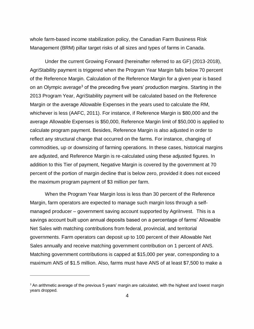
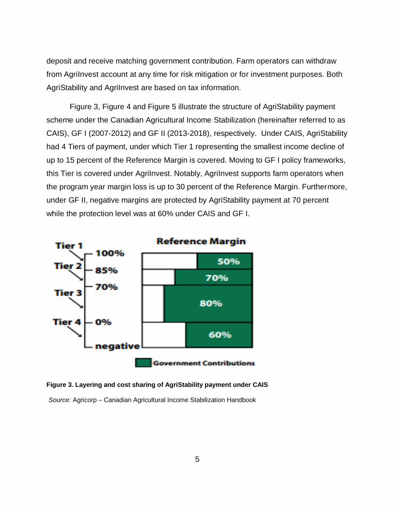
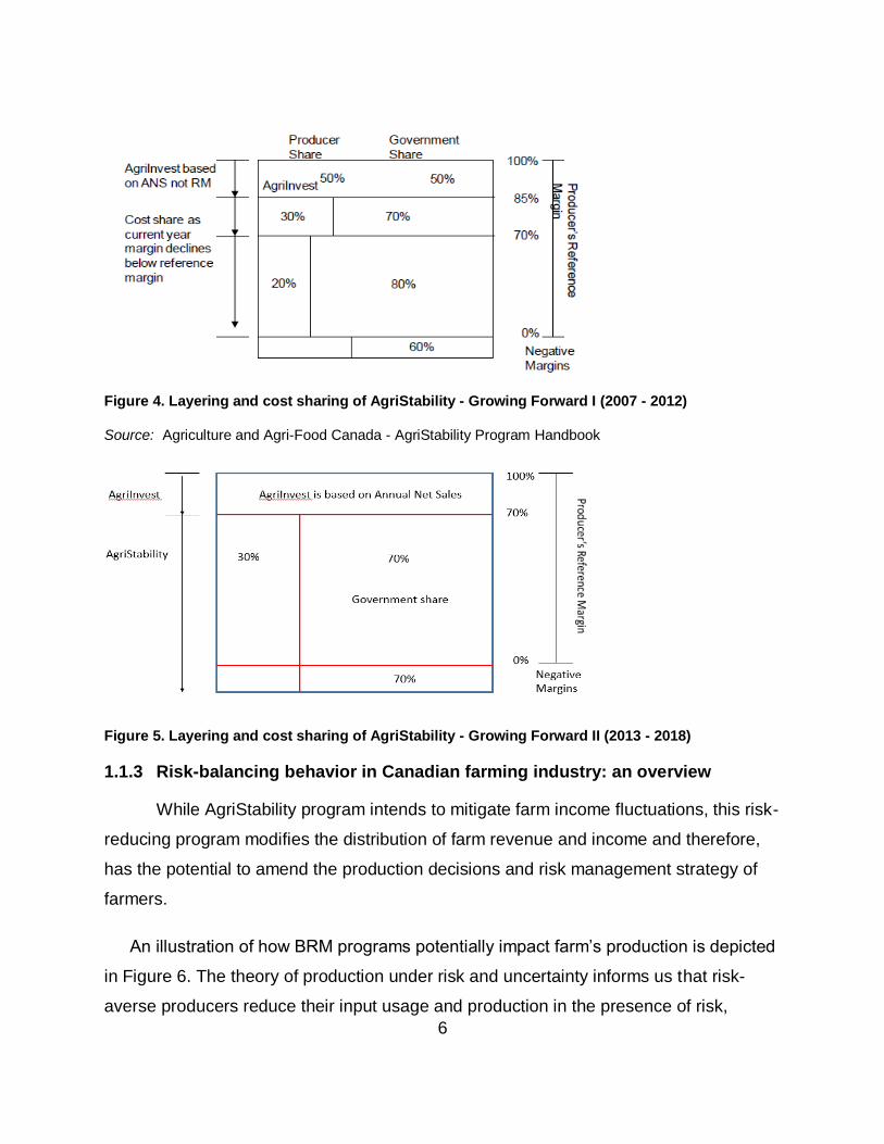
Figure 3, Figure 4 and Figure 5 illustrate the structure of AgriStability payment

scheme under the Canadian Agricultural Income Stabilization (hereinafter referred to as

CAIS), GF I (2007-2012) and GF II (2013-2018), respectively. Under CAIS, AgriStability

had 4 Tiers of payment, under which Tier 1 representing the smallest income decline of

up to 15 percent of the Reference Margin is covered. Moving to GF I policy frameworks,

this Tier is covered under AgriInvest. Notably, AgriInvest supports farm operators when

the program year margin loss is up to 30 percent of the Reference Margin. Furthermore,

under GF II, negative margins are protected by AgriStability payment at 70 percent

while the protection level was at 60% under CAIS and GF I.

Figure 3. Layering and cost sharing of AgriStability payment under CAIS

Source: Agricorp – Canadian Agricultural Income Stabilization Handbook

6

Figure 4. Layering and cost sharing of AgriStability - Growing Forward I (2007 - 2012)

Source: Agriculture and Agri-Food Canada - AgriStability Program Handbook

Figure 5. Layering and cost sharing of AgriStability - Growing Forward II (2013 - 2018)

1.1.3 Risk-balancing behavior in Canadian farming industry: an overview

While AgriStability program intends to mitigate farm income fluctuations, this risk-

reducing program modifies the distribution of farm revenue and income and therefore,

has the potential to amend the production decisions and risk management strategy of

farmers.

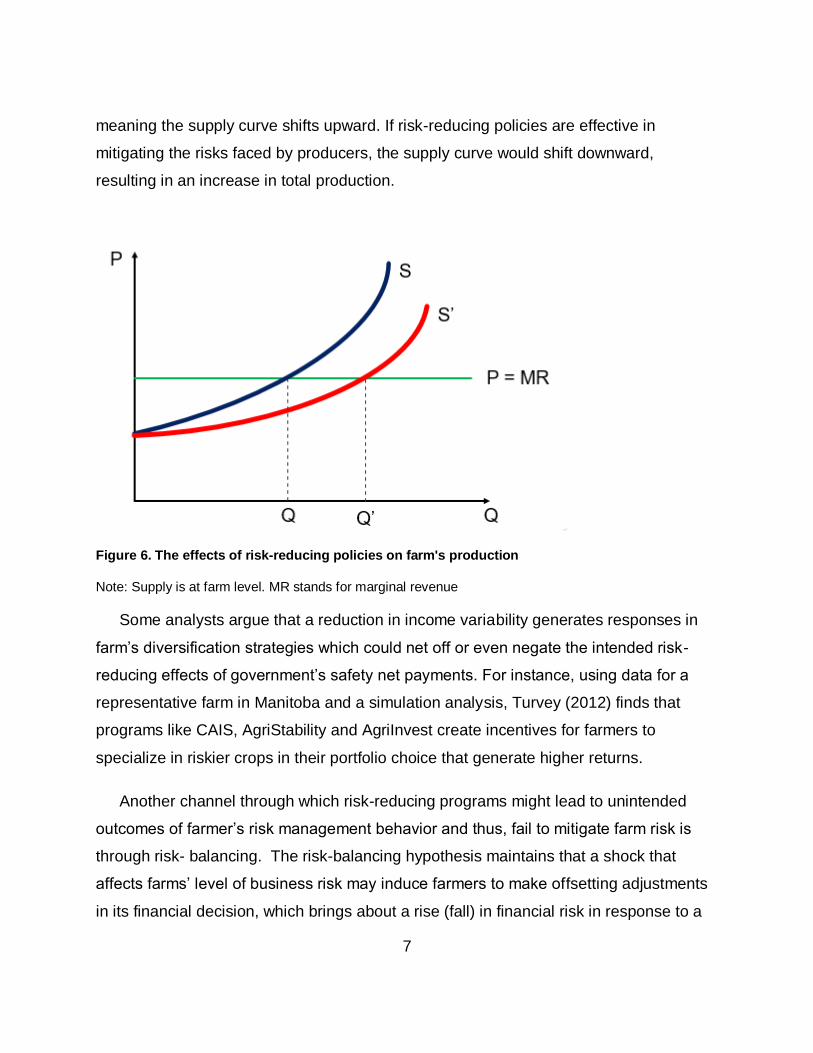
An illustration of how BRM programs potentially impact farm’s production is depicted

in Figure 6. The theory of production under risk and uncertainty informs us that risk-

averse producers reduce their input usage and production in the presence of risk,

7

meaning the supply curve shifts upward. If risk-reducing policies are effective in

mitigating the risks faced by producers, the supply curve would shift downward,

resulting in an increase in total production.

Figure 6. The effects of risk-reducing policies on farm's production

Note: Supply is at farm level. MR stands for marginal revenue

Some analysts argue that a reduction in income variability generates responses in

farm’s diversification strategies which could net off or even negate the intended risk-

reducing effects of government’s safety net payments. For instance, using data for a

representative farm in Manitoba and a simulation analysis, Turvey (2012) finds that

programs like CAIS, AgriStability and AgriInvest create incentives for farmers to

specialize in riskier crops in their portfolio choice that generate higher returns.

Another channel through which risk-reducing programs might lead to unintended

outcomes of farmer’s risk management behavior and thus, fail to mitigate farm risk is

through risk- balancing. The risk-balancing hypothesis maintains that a shock that

affects farms’ level of business risk may induce farmers to make offsetting adjustments

in its financial decision, which brings about a rise (fall) in financial risk in response to a

8

fall (rise) in business risk (Gabriel & Baker, 1980). This could lead to an increase

(decrease) rather than decrease (increase) of overall farm risks.

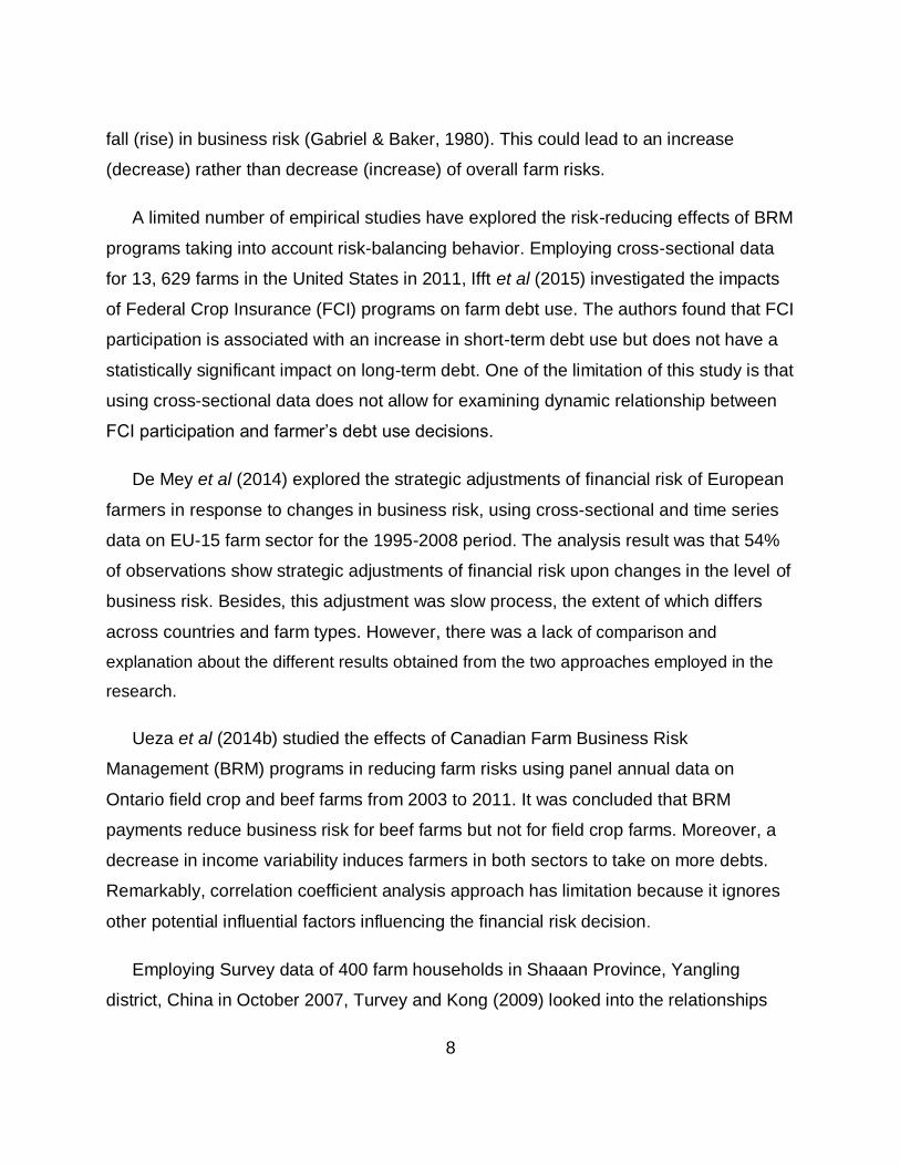
A limited number of empirical studies have explored the risk-reducing effects of BRM

programs taking into account risk-balancing behavior. Employing cross-sectional data

for 13, 629 farms in the United States in 2011, Ifft et al (2015) investigated the impacts

of Federal Crop Insurance (FCI) programs on farm debt use. The authors found that FCI

participation is associated with an increase in short-term debt use but does not have a

statistically significant impact on long-term debt. One of the limitation of this study is that

using cross-sectional data does not allow for examining dynamic relationship between

FCI participation and farmer’s debt use decisions.

De Mey et al (2014) explored the strategic adjustments of financial risk of European

farmers in response to changes in business risk, using cross-sectional and time series

data on EU-15 farm sector for the 1995-2008 period. The analysis result was that 54%

of observations show strategic adjustments of financial risk upon changes in the level of

business risk. Besides, this adjustment was slow process, the extent of which differs

across countries and farm types. However, there was a lack of comparison and

explanation about the different results obtained from the two approaches employed in the

research.

Ueza et al (2014b) studied the effects of Canadian Farm Business Risk

Management (BRM) programs in reducing farm risks using panel annual data on

Ontario field crop and beef farms from 2003 to 2011. It was concluded that BRM

payments reduce business risk for beef farms but not for field crop farms. Moreover, a

decrease in income variability induces farmers in both sectors to take on more debts.

Remarkably, correlation coefficient analysis approach has limitation because it ignores

other potential influential factors influencing the financial risk decision.

Employing Survey data of 400 farm households in Shaaan Province, Yangling

district, China in October 2007, Turvey and Kong (2009) looked into the relationships

9

between business risks and credit choices of rural farm households in China. Findings

were that farmers' credit choices are related to expected production risk, risk aversion

and expected farm income. Also, farmers facing higher production risks reduce financial

risks with lower credit demand. A point to note, the paper did not give sufficient

explanation of the different results obtained from the four regressions.

Escalante and Barry (2003) explore the strength of trade-offs between business risk

and financial risk using panel farm-level dataset of 80 farms over the 1982-1998 period

in the United States. The authors concluded that 50% of farms showed strategic

adjustment of capital structure when the level of business risk changes. Also, amount of

crop insurance coverage, farm tenure position and crop diversification are determinants

of the strategic capital adjustments. This paper provides motivation for investigating the

extent of risk reduction realized under a more integrated risk management approach,

given the compatibility between risk balancing and alternative strategies demonstrated

in this study.

A critical review of the existing empirical literature on risk-balancing behavior will be

provided in Chapter 3 – Literature Review. In this chapter, specific questions pertaining

to each empirical study will also be addressed, including but not limit to: whether the

authors use an appropriate analytical framework and whether the empirical analysis is

adequate; any limitations in the econometric methods used and how could those be

improved; gap(s) highlighting and how those gaps could be bridged in this thesis.

1.2 Economic problem, economic research problem and motivation for the study

The following section presents economic problem, economic research problem and

specifies the scope of this study.

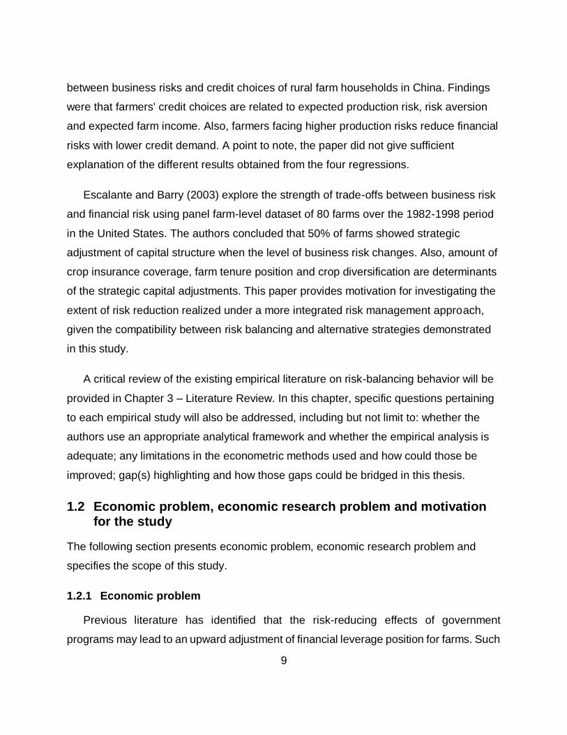
1.2.1 Economic problem

Previous literature has identified that the risk-reducing effects of government

programs may lead to an upward adjustment of financial leverage position for farms. Such

10

responses, if present, may offset the desirable benefits of BRM programs and may make

the program ineffective in the long run. This could also adversely affect the long-run

sustainability of farming in Canada.

This research will investigate the risk-balancing behavior of farmers in the Ontario hog

sector as a result of AgriStability payments under CAIS/ BRM programs. Therefore, its

result could be of interests to the administrators of BRM programs, who are to review and

make necessary adjustments to these programs upon the expiration of Growing Forward

II in 2018 so that the intended objective of mitigating farm risks could be attained. Put

differently, the findings of this research on the effectiveness of BRM programs in reducing

farm risks, taking into account the possible risk-balancing behaviors of farmers, would

encourage the government at federal, provincial and territorial level4 to either continue

mitigating farm risks for the Ontario hog sector through this channel or consider making

necessary amendments to these programs or even explore other policy change to reduce

farm risks.

1.2.2 Economic research problem

It is not known from the existing empirical literature if Canadian farm BRM

programs reduce business risk for Ontario hog farms. Furthermore, the ways business

risk was measured varies across studies, and each way has its own pros and cons.

Besides, it is not known whether this reduction in business risk leads to an increase in

financial risk and possibly, a higher level of overall risk for farm operations. Additionally,

against the current background of increasing farm consolidation, a question of interest

has arisen on whether the extent of risk-balancing differs among farms of different size

categories.

In addition, there is more than one channel through which farmers may perform

their risk management behaviors that may crowd out the risk-reducing effects of BRM

4 Growing Forward 2 is a five-year policy frame-work (2013-2018) for Canada agriculture and agri-food

sector based on the investment of federal, provincial and territorial governments.

11

programs. Findings from Escalante and Barry (2003) suggest that if risk-reducing

policies reduce farmer’s incentive to buy Crop Insurance, insurance-protection plans

could be considered as an alternative to risk-balancing. This means that instead of

making offsetting adjustment in farm’s leverage position by taking on more debt,

farmers may respond to the reduction in business risk level as a result of government’s

financial aid by purchasing less Crop Insurance. This could generate a higher level of

overall risk for farm operations. However, little is known from the current literature on

whether or not this behavior is prevalent among hog farm operators in Ontario. Put

differently, it is not known whether Crop Insurance and BRM/ AgriStability are

substitutes or complements in program participation.

This research builds upon the theoretical framework conceptualized by Gabriel and

Barker (1980) and Collins (1985).

This economic research problem falls under the category of a policy evaluation.

BRM programs are under the umbrella of Growing Forward, an agricultural policy

framework subject to evaluation and revision every five years in Canada. The scope of

this study is limited to the Ontario hog sector for the 2003-2014 period.

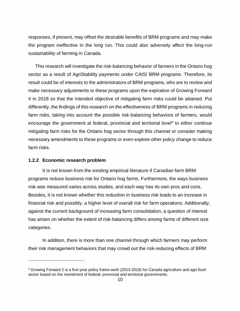
1.2.3 Motivation for the study: why Ontario hog sector?

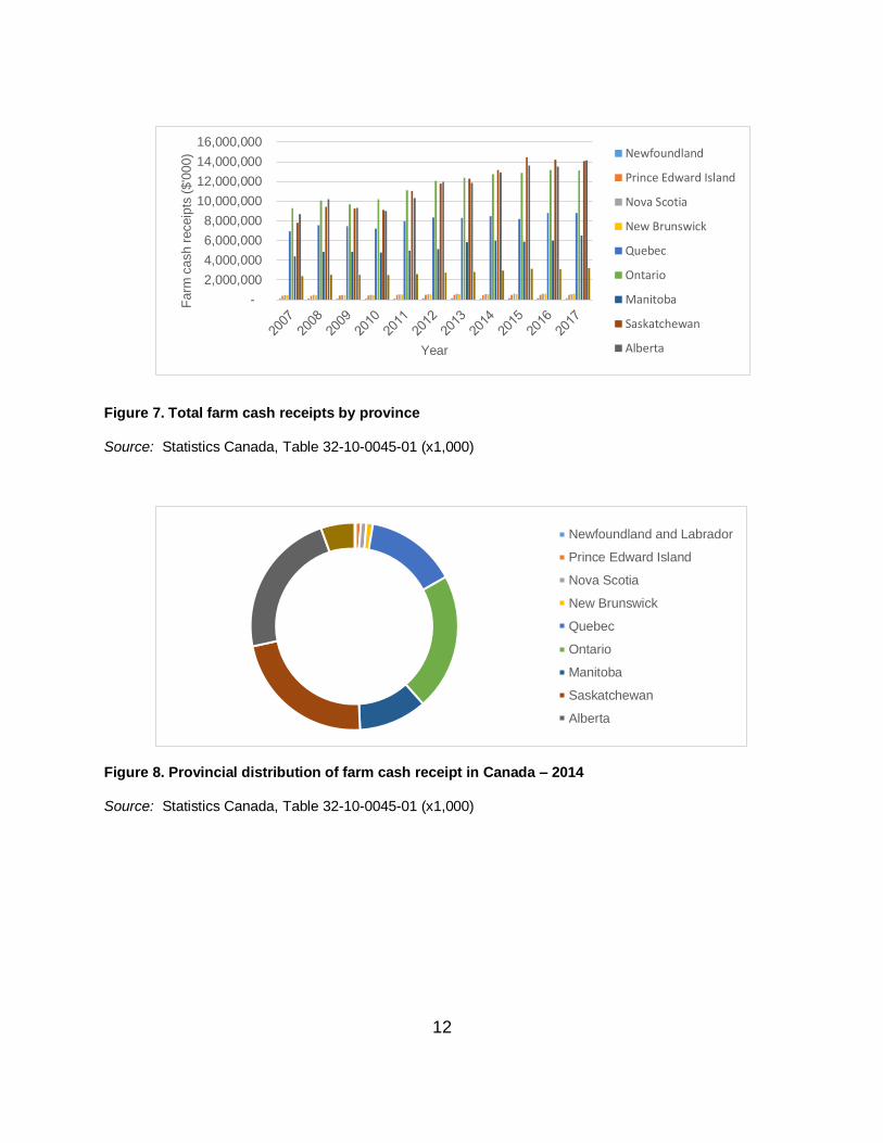
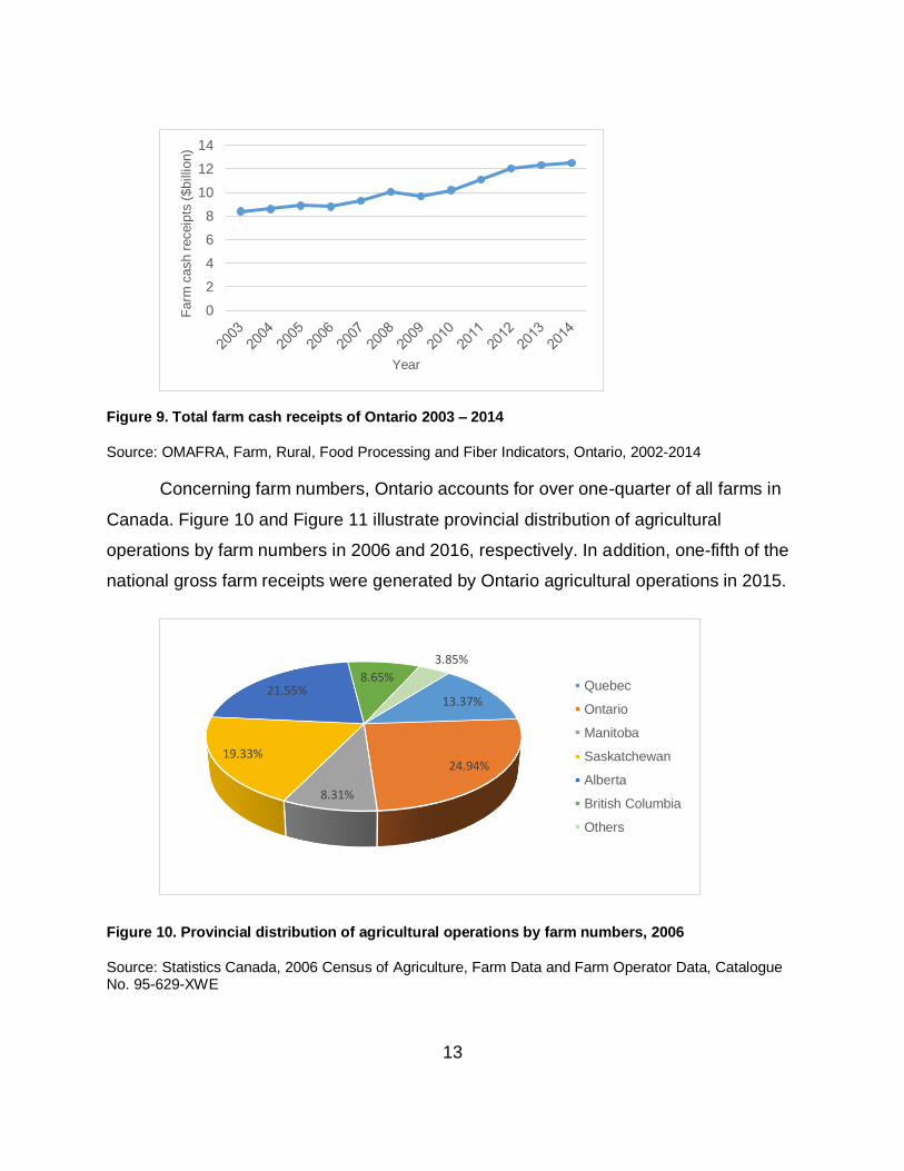
Ontario continues to hold a strong position in the Canadian agri-food landscape.

The province ranks 3rd following Saskatchewan and Alberta in terms of farm cash

receipts over years and accounts for more than 20 percent of farm cash receipts of

Canada. Figure 7 demonstrates farm cash receipts by province from 2007 to 2017 and

Figure 8 depicts provincial distribution of total farm cash receipts in 2014. Besides,

Ontario farm cash receipts followed a consistent upward sloping trend during the study

period (Fig. 9).

12

Figure 7. Total farm cash receipts by province

Source: Statistics Canada, Table 32-10-0045-01 (x1,000)

Figure 8. Provincial distribution of farm cash receipt in Canada – 2014

Source: Statistics Canada, Table 32-10-0045-01 (x1,000)

-

2,000,000

4,000,000

6,000,000

8,000,000

10,000,000

12,000,000

14,000,000

16,000,000

Farm

cash r

eceip

ts (

$'0

00)

Year

Newfoundland

Prince Edward Island

Nova Scotia

New Brunswick

Quebec

Ontario

Manitoba

Saskatchewan

Alberta

Newfoundland and Labrador


Nova Scotia

New Brunswick

Quebec

Ontario

Manitoba

Saskatchewan

Alberta

13

Figure 9. Total farm cash receipts of Ontario 2003 – 2014

Source: OMAFRA, Farm, Rural, Food Processing and Fiber Indicators, Ontario, 2002-2014

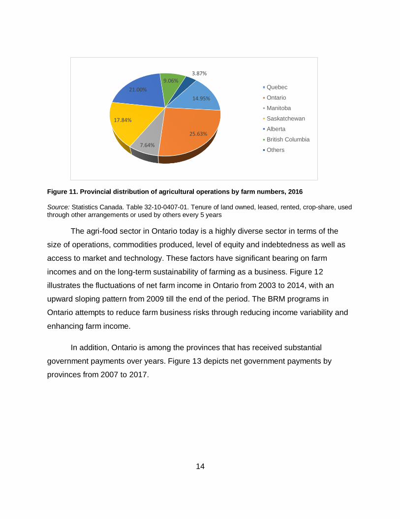
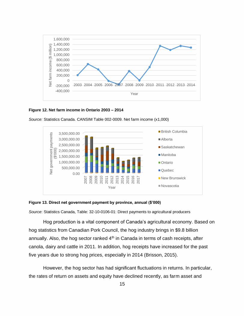
Concerning farm numbers, Ontario accounts for over one-quarter of all farms in

Canada. Figure 10 and Figure 11 illustrate provincial distribution of agricultural

operations by farm numbers in 2006 and 2016, respectively. In addition, one-fifth of the

national gross farm receipts were generated by Ontario agricultural operations in 2015.

Figure 10. Provincial distribution of agricultural operations by farm numbers, 2006

Source: Statistics Canada, 2006 Census of Agriculture, Farm Data and Farm Operator Data, Catalogue No. 95-629-XWE

0

2

4

6

8

10

12

14

Farm

cash r

eceip

ts (

$billion)

Year

13.37%

24.94%

8.31%

19.33%

21.55%8.65%

3.85%

Quebec

Ontario

Manitoba

Saskatchewan

Alberta

British Columbia

Others

14

Figure 11. Provincial distribution of agricultural operations by farm numbers, 2016

Source: Statistics Canada. Table 32-10-0407-01. Tenure of land owned, leased, rented, crop-share, used through other arrangements or used by others every 5 years

The agri-food sector in Ontario today is a highly diverse sector in terms of the

size of operations, commodities produced, level of equity and indebtedness as well as

access to market and technology. These factors have significant bearing on farm

incomes and on the long-term sustainability of farming as a business. Figure 12

illustrates the fluctuations of net farm income in Ontario from 2003 to 2014, with an

upward sloping pattern from 2009 till the end of the period. The BRM programs in

Ontario attempts to reduce farm business risks through reducing income variability and

enhancing farm income.

In addition, Ontario is among the provinces that has received substantial

government payments over years. Figure 13 depicts net government payments by

provinces from 2007 to 2017.

14.95%

25.63%

7.64%

17.84%

21.00%

9.06%3.87%

Quebec

Ontario

Manitoba

Saskatchewan

Alberta

British Columbia

Others

15

Figure 12. Net farm income in Ontario 2003 – 2014

Source: Statistics Canada. CANSIM Table 002-0009. Net farm income (x1,000)

Figure 13. Direct net government payment by province, annual ($’000)

Source: Statistics Canada, Table: 32-10-0106-01: Direct payments to agricultural producers

Hog production is a vital component of Canada’s agricultural economy. Based on

hog statistics from Canadian Pork Council, the hog industry brings in $9.8 billion

annually. Also, the hog sector ranked 4th in Canada in terms of cash receipts, after

canola, dairy and cattle in 2011. In addition, hog receipts have increased for the past

five years due to strong hog prices, especially in 2014 (Brisson, 2015).

However, the hog sector has had significant fluctuations in returns. In particular,

the rates of return on assets and equity have declined recently, as farm asset and

-400,000

-200,000

0

200,000

400,000

600,000

800,000

1,000,000

1,200,000

1,400,000

1,600,000

2003 2004 2005 2006 2007 2008 2009 2010 2011 2012 2013 2014Net

farm

incom

e ($ m

illio

n)

Year

0.00

500,000.00

1,000,000.00

1,500,000.00

2,000,000.00

2,500,000.00

3,000,000.00

3,500,000.00

2007

2008

2009

2010

2011

2012

2013

2014

2015

2016

2017

Net

govern

ment paym

ents

($

'000)

Year

British Columbia

Alberta

Saskatchewan

Manitoba

Ontario

Quebec

New Brunswick

Novascotia

16

equity values have increased faster than net incomes. Increased asset values partly

reflect the general increase in the size of hog farms across provinces in Canada.

Most importantly, Ontario is among the three provinces that dominates hog and

pork production in Canada. Sectoral highlights in the province will be presented and

elaborated with key facts and feature under section 2.6 in the next chapter.

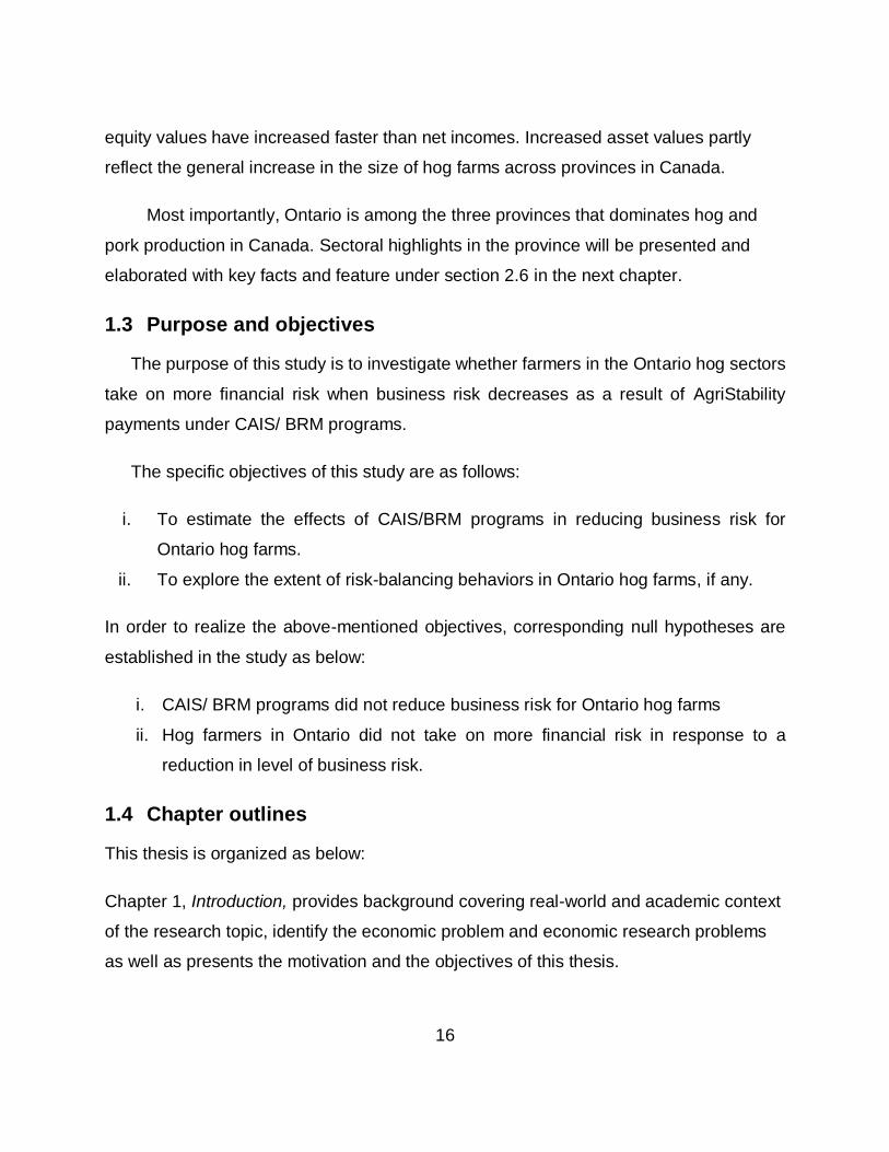
1.3 Purpose and objectives

The purpose of this study is to investigate whether farmers in the Ontario hog sectors

take on more financial risk when business risk decreases as a result of AgriStability

payments under CAIS/ BRM programs.

The specific objectives of this study are as follows:

i. To estimate the effects of CAIS/BRM programs in reducing business risk for

Ontario hog farms.

ii. To explore the extent of risk-balancing behaviors in Ontario hog farms, if any.

In order to realize the above-mentioned objectives, corresponding null hypotheses are

established in the study as below:

i. CAIS/ BRM programs did not reduce business risk for Ontario hog farms

ii. Hog farmers in Ontario did not take on more financial risk in response to a

reduction in level of business risk.

1.4 Chapter outlines

This thesis is organized as below:

Chapter 1, Introduction, provides background covering real-world and academic context

of the research topic, identify the economic problem and economic research problems

as well as presents the motivation and the objectives of this thesis.

17

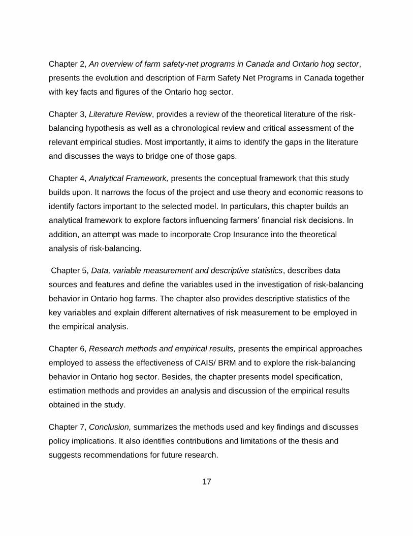
Chapter 2, An overview of farm safety-net programs in Canada and Ontario hog sector,

presents the evolution and description of Farm Safety Net Programs in Canada together

with key facts and figures of the Ontario hog sector.

Chapter 3, Literature Review, provides a review of the theoretical literature of the risk-

balancing hypothesis as well as a chronological review and critical assessment of the

relevant empirical studies. Most importantly, it aims to identify the gaps in the literature

and discusses the ways to bridge one of those gaps.

Chapter 4, Analytical Framework, presents the conceptual framework that this study

builds upon. It narrows the focus of the project and use theory and economic reasons to

identify factors important to the selected model. In particulars, this chapter builds an

analytical framework to explore factors influencing farmers’ financial risk decisions. In

addition, an attempt was made to incorporate Crop Insurance into the theoretical

analysis of risk-balancing.

Chapter 5, Data, variable measurement and descriptive statistics, describes data

sources and features and define the variables used in the investigation of risk-balancing

behavior in Ontario hog farms. The chapter also provides descriptive statistics of the

key variables and explain different alternatives of risk measurement to be employed in

the empirical analysis.

Chapter 6, Research methods and empirical results, presents the empirical approaches

employed to assess the effectiveness of CAIS/ BRM and to explore the risk-balancing

behavior in Ontario hog sector. Besides, the chapter presents model specification,

estimation methods and provides an analysis and discussion of the empirical results

obtained in the study.

Chapter 7, Conclusion, summarizes the methods used and key findings and discusses

policy implications. It also identifies contributions and limitations of the thesis and

suggests recommendations for future research.

18

2 CHAPTER 2. AN OVERVIEW OF CANADIAN FARM SAFETY-NET PROGRAMS AND ONTARIO HOG SECTOR

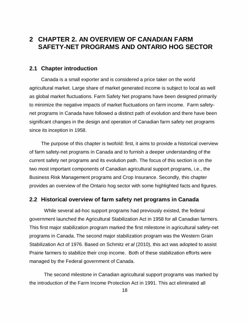
2.1 Chapter introduction

Canada is a small exporter and is considered a price taker on the world

agricultural market. Large share of market generated income is subject to local as well

as global market fluctuations. Farm Safety Net programs have been designed primarily

to minimize the negative impacts of market fluctuations on farm income. Farm safety-

net programs in Canada have followed a distinct path of evolution and there have been

significant changes in the design and operation of Canadian farm safety net programs

since its inception in 1958.

The purpose of this chapter is twofold: first, it aims to provide a historical overview

of farm safety-net programs in Canada and to furnish a deeper understanding of the

current safety net programs and its evolution path. The focus of this section is on the

two most important components of Canadian agricultural support programs, i.e., the

Business Risk Management programs and Crop Insurance. Secondly, this chapter

provides an overview of the Ontario hog sector with some highlighted facts and figures.

2.2 Historical overview of farm safety net programs in Canada

While several ad-hoc support programs had previously existed, the federal

government launched the Agricultural Stabilization Act in 1958 for all Canadian farmers.

This first major stabilization program marked the first milestone in agricultural safety-net

programs in Canada. The second major stabilization program was the Western Grain

Stabilization Act of 1976. Based on Schmitz et al (2010), this act was adopted to assist

Prairie farmers to stabilize their crop income. Both of these stabilization efforts were

managed by the Federal government of Canada.

The second milestone in Canadian agricultural support programs was marked by

the introduction of the Farm Income Protection Act in 1991. This act eliminated all

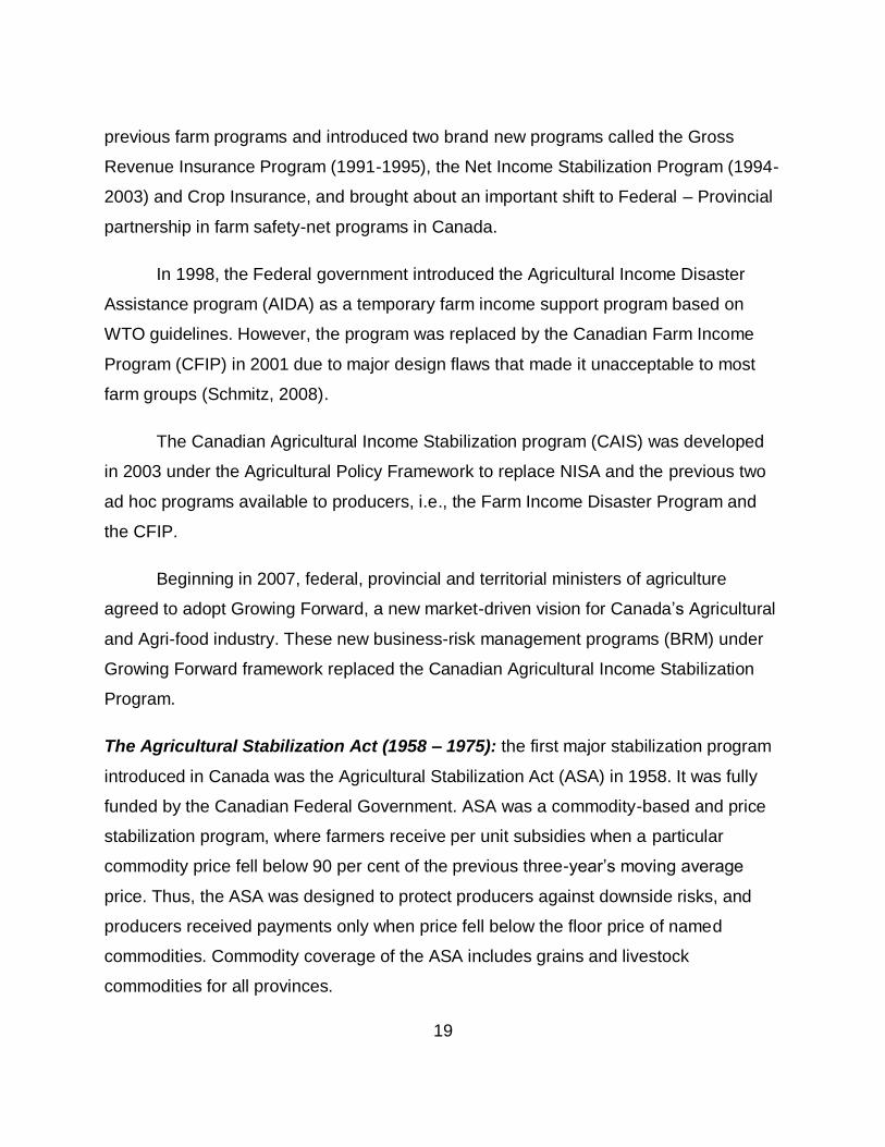
19

previous farm programs and introduced two brand new programs called the Gross

Revenue Insurance Program (1991-1995), the Net Income Stabilization Program (1994-

2003) and Crop Insurance, and brought about an important shift to Federal – Provincial

partnership in farm safety-net programs in Canada.

In 1998, the Federal government introduced the Agricultural Income Disaster

Assistance program (AIDA) as a temporary farm income support program based on

WTO guidelines. However, the program was replaced by the Canadian Farm Income

Program (CFIP) in 2001 due to major design flaws that made it unacceptable to most

farm groups (Schmitz, 2008).

The Canadian Agricultural Income Stabilization program (CAIS) was developed

in 2003 under the Agricultural Policy Framework to replace NISA and the previous two

ad hoc programs available to producers, i.e., the Farm Income Disaster Program and

the CFIP.

Beginning in 2007, federal, provincial and territorial ministers of agriculture

agreed to adopt Growing Forward, a new market-driven vision for Canada’s Agricultural

and Agri-food industry. These new business-risk management programs (BRM) under

Growing Forward framework replaced the Canadian Agricultural Income Stabilization

Program.

The Agricultural Stabilization Act (1958 – 1975): the first major stabilization program

introduced in Canada was the Agricultural Stabilization Act (ASA) in 1958. It was fully

funded by the Canadian Federal Government. ASA was a commodity-based and price

stabilization program, where farmers receive per unit subsidies when a particular

commodity price fell below 90 per cent of the previous three-year’s moving average

price. Thus, the ASA was designed to protect producers against downside risks, and

producers received payments only when price fell below the floor price of named

commodities. Commodity coverage of the ASA includes grains and livestock

commodities for all provinces.

20

It is interesting to note that Crop Insurance programs have been a part of Canadian

agricultural policy since it was launched under the Canadian Insurance Act in 1957 and

it co-existed with the ASA for most the period.

The Western Grain Stabilization Act (1976-1991): according to Schmitz et al (2010),

the Western Grain Stabilization Act (WGSA) was proposed to stabilize aggregate net

cash flow for special grains. Thus, together with the crop insurance, which was to even

out yield, these two programs were designed to stabilize income. By design, the support

level under WGSA was calculated using a 3-year moving average of market returns.

The sharp decline in world grain prices in 1985 triggered a large payout under the

WGSA. As a result, the program could not be maintained in an actuarially sound

manner after five years of implementation. It was dismantled under the Farm Income

Protection Act (hereinafter referred to as FIPA) in 1991.

FIPA had three components: the Gross Revenue Insurance Program (GRIP), the

Net Income Stabilization Account (NISA) and Crop Insurance (CI). The introduction of

the FIPA made a significant change in Canadian agricultural policy (Schmitz, 2008).

Under FIPA, provinces were required to contribute their part to the funding of the farm-

income support programs.

Gross Revenue Insurance Program (1991-1995): launched in 1991, the Gross

Revenue Insurance Program (GRIP) was a commodity-specific program that operated

through a tripartite-funding scheme. GRIP was designed to protect crop farmers against

the negative effects of yield or price shortfalls by guaranteeing a per acre gross return.

However, GRIP had two major problems that led to its downfall starting in 1992 by the

withdrawal from the program by Saskatchewan government. (Schmitz et al, 2010).

These authors argued that GRIP was expensive. In particular, given the large portion of

cost born by the provincial government relative to the previous programs, it was hard for

provinces with large land base and sparse population to afford this tripartite program.

Moreover, GRIP has the potential for moral hazard and adverse selection. Put

21

differently, the program could not remain actuarially sound due to its design and was

finally dismantled after five years of operation.

The Net Income Stabilization Account (1990-2003): introduced under FIPA, the Net

Income Stabilization Account (NISA) was the first safety-net program with whole-farm

approach. NISA had a three-party funding calculation, with cost-shared 50-50 between

government (federal and provincial combined) and producers. According to Schmitz et

al (2010), NISA established special saving accounts where producers could deposit up

to 2 percent of their eligible net sale and receive a matching contribution from the

government. Participating farm operators were also paid a 3 percent interest premium

over the prevailing market rates.

Producers could make withdrawals from NISA accounts under two conditions.

The first condition was if farm income fell below 70 percent of the previous 5-year

average. The second condition was if the farmer’s net farm income fell below

CAD10,000, or CAD 20,000 for farmers with dependents. These thresholds were later

increased to CAD20,000 and CAD35,000, respectively (Anton, Kimura & Martini, 2011).

The drawbacks of NISA were two-fold: firstly, farmers found it wasteful to have a

large part of their capital tied up in the program; secondly, from the government’s

perspective, the large balances held in NISA accounts suggested that those funds were

not utilized to stabilize income as originally intended. These factors led to NISA being

replaced and embedded with some changes later on in the Canadian Agricultural

Income Stabilization program.

The Canadian Agricultural Income Stabilization program (2003-2007): based on

AAFC (2005), Agriculture and Agri-Food Canada and all provinces and territories signed

the five-year Agricultural Policy Framework (APF) agreement in 2003 to realize the

objective of making Canada the world leader in food safety, innovation and

environmentally-responsible production. The introduction of APF was an attempt by the

federal government and provinces to generate a more integrated approach to

22

agricultural policy against the background of a growing number of programs operating at

all levels of government.

Introduced under the APF, CAIS was designed as a whole farm based program

to protect farming operations from both small and large drops in income. The program

formed the central risk-management program and was based for the first time on net

margin. In particular, payments depend on current versus reference margin equal to

five-year Olympic average. When the margin fell below the reference margin, producers

receive program payments depending on the size of the shortfall relative to the

reference margin and coverage level. Figure 3 illustrates the structure of AgriStability

payment scheme under CAIS.

Program payments cannot exceed 70 percent of the total margin decline and is

capped at $3 million for a given program year. Also, CAIS was modified in 2004 to

include coverage for negative margin to compensate for losses as well as reduction in

income. Under this modification, the requirement for producers to deposit one-third of

the insured amount was eliminated.

The main difference between NISA and CAIS was that the matching government

contribution to the account under CAIS was not made at the time of deposit, but when

the funds were withdrawn. This was intended to address the accumulation of large

account balance as one of the drawback of NISA (Anton, Kimura & Martini, 2011).

The Canadian Business Risk Management programs under Growing Forward

framework: in 2007, federal, provincial and territorial ministers of agriculture agreed to

adopt Growing Forward (GF), a market-driven vision for Canada’s agriculture and agri-

food industry. The GF framework is an evolution from the APF in the sense that the

former “eliminated the provincial ‘companion’ programs institutionalized when NISA was

established and allowing provinces to supplement federal-provincial initiatives if

desired…” (Anton, Kimura & Martini, 2011, p. 24). Also, it defines the current set of

23

policies in Canada and attempts to define different layers of public response to risk in

agriculture and includes the following four components:

AgriInvest: being the successor of NISA, AgriInvest is a producer savings account that

was designed to stabilize year-to-year small fluctuations in income as well as support

investment to mitigate risk and improve income. AgriInvest account builds as producers

make annual deposits based on a percentage of their Allowable Net Sales (ANS) and

receive matching contributions from federal, provincial, and territorial governments.

Program details, including coverage levels, pricing options, commodity coverage varies

by province, and administration of the program is primarily done at the provincial level.

AgriStability: this whole farm and margin-based component evolved out of CAIS. Under

this component, participating producers are eligible for an AgriStability payout if their

Program Margin, i.e., eligible revenue minus eligible expenses, falls below a Reference

Margin. The Reference Margin is a historical average of Program Margins. An Olympic

average is used to calculate the Program Margin. Under AgriStability, individual

information is gathered from tax files and complemented with additional information

from farmers. This process takes a great deal of time and could create delays and

uncertainty about the timing and amount of the payout.

Both AgiStability and AgriInvest are comprehensive in terms of the risks and

sources they cover, meaning these components cover risks that are normal but are also

available when risks become more catastrophic. The authors maintained that normal

risks and catastrophic risks can be defined based on the frequency and type of events

occurring. In this light, the standard layer refers to frequent and small events while rare

and large events belongs to catastrophic layer.

Figure 14 illustrates different risk layering covered by Canadian risk management

programs. As can be seen from this diagram, coverage under AgriStability from layer 2

to layer 4 proves to be quite comprehensive in addressing both normal and catastrophic

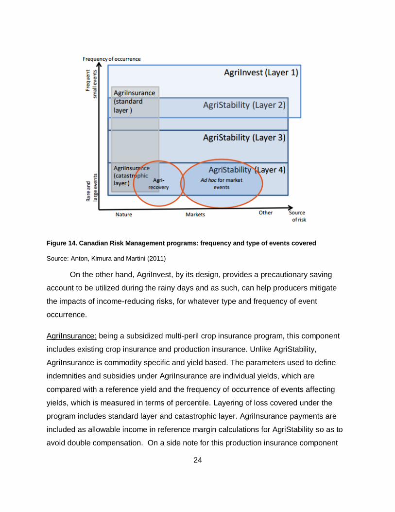
24

Figure 14. Canadian Risk Management programs: frequency and type of events covered

Source: Anton, Kimura and Martini (2011)

On the other hand, AgriInvest, by its design, provides a precautionary saving

account to be utilized during the rainy days and as such, can help producers mitigate

the impacts of income-reducing risks, for whatever type and frequency of event

occurrence.

AgriInsurance: being a subsidized multi-peril crop insurance program, this component

includes existing crop insurance and production insurance. Unlike AgriStability,

AgriInsurance is commodity specific and yield based. The parameters used to define

indemnities and subsidies under AgriInsurance are individual yields, which are

compared with a reference yield and the frequency of occurrence of events affecting

yields, which is measured in terms of percentile. Layering of loss covered under the

program includes standard layer and catastrophic layer. AgriInsurance payments are

included as allowable income in reference margin calculations for AgriStability so as to

avoid double compensation. On a side note for this production insurance component

25

under BRM suite, Ontario is one of the provinces where AgriInsurance also includes

livestock price insurance.

AgriRecovery: this is a disaster-relief framework designed to provide direct payment in

the event of a large-scale farm income disaster (Vercarmmen, 2013). This component

under BRM suite is aimed to cover catastrophic risks and supposed to be the main

catastrophic risk management instrument in Canada. AgriRecovery is structured with a

disaster layer for natural events that affect production and support is decided on by

provincial and federal governments over consultation process.

2.3 BRM program under Growing Forward II (2013-2017)

While there were no significant changes to either AgriInsurance or AgriRecovery

under GF II, AgriStability and AgriInvest parameters were changed and reflected a

reduction in government support.

Regarding AgriInvest, the rules governing producer deposit and matching

contributions from government changed. In particular, starting with the 2013 program

year, producers can deposit up to 100% of their annual ANS, with the first 1% matched

by governments. Matching government contributions was capped at $15,000 per year

compared to $22,500 under GF I (AAFC, 2017). Also, the maximum account balance

limit including matching deposits, government contributions and interests earned was

increased from 25 percent of historical average ANS to 400 percent of ANS. According

to Jeffrey (2015), these changes brought about greater flexibility for producers in

reserving funds for future withdrawals to cope with income shortfalls. Simultaneously,

they reflect reduced government support under the form of matching contributions.

With respect to AgriStability, there were four changes under GF II. Firstly, the

degree of decline in the Program Year Margin required to trigger a payout was

increased from 15 percent to 30 percent, meaning that there was no payout until the

Program Year Margin fell to 70 percent of the Reference Margin. Secondly, the

coverage level no longer depended on the degree of decline; AgriStability payouts were

26

equal to 70 percent of the eligible decline. Finally, calculation for the Reference Margin

used to determine eligibility for an AgriStability payout was now the lesser of the

historical average Program Margin and the historical average of allowable expenses

(Jeffrey, 2015). Finally, negative margin are protected by AgriStability payment at 70

percent under GF II while the protection level is 60 percent under CAIS and GF I.

Notably, a decline in the program year margin relative to the Reference Margin is

not required for producers to withdraw from their AgriInvest account. In particular, when

the program year margin falls less than 15 percent of the Reference Margin under GF I

or less than 30 percent of the Reference Margin under GF II, program payment is not

triggered and thus, producers may withdraw from their AgriInvest accounts as a source

of self-risk managing.

Overall, the changes in parameters of the AgriStability component had different

directional impacts on the likelihood and amount of the program payouts but likely

resulted in reduced capacity to support and stabilize farm incomes.

In a nutshell, being the core of Canadian agricultural policies, BRM programs

covers a large set of measures for risk reduction, mitigation and coping that are aimed

to smooth income from farming. Besides, while some of the components under BRM

suites are ex ante measures, some others are payments triggered ex post. For

instance, AgriInsurance and AgriInvest are considered as ex ante measures while

countercyclical payouts under AgriStability are triggered ex post by government using

tax record. In a similar vein, as support under AgriRecovery is decided over consultation

process and based on non-defined specific criteria, they are considered as payments

decided upon ex post.

Agriculture faces risks of several sources and that all of these sources of risk

eventually translate or manifest into farm income risk. The policy priority for BRM

programs is, therefore, to help stabilize farm income (Anton, Kimura & Martini, 2011). In

this regard, AgriStability, the successor of CAIS remains the center of Canadian

27

agricultural risk management strategy and AgriStability payouts will be examined and

incorporated into analysis in this research.

2.4 Crop Insurance Program

The goverment of Canada introduced and passed the Crop Insurance Act in 1959.

It provided enabling legislation for provincial governments to establish crop insurance

programs that obtained financial support from the federal government. Since its inception,

crop insurance has remained a joint federal-provincial program. According to Schmitz et

al (2010), Crop insurance is available to individual producers based on individual farm

yields, and covers grains, pulses, oilseeds, and forages. The payouts from crop insurance

vary from year to year, since price coverage varies according to market conditions.

Since insurance coverage decreases as commodity prices fall, Crop insurance

cannot support farm income to any major degree during periods of depressed prices.

Remarkably, Crop Insurance in Canada has always been a government program with no

involvement of specialized private insurers and it is managed like a program of payments

to farmers rather than an insurance business, even if farmers have to contribute with part

the premium (Anton, Kimura & Martini, 2011, p.39). The authors also maintain that

government and their agencies have continually refined policies to increase commodity

coverage and increase the share of the premium paid by the government.

Participation rate has always been an important consideration in the design of crop

insurance programs. The main vehicle by which the government can control participation

rates is the extent to which the premium is subsidized. Participation rates vary by province

as well as regions within the provinces. Farmers in regions with high yield variance had

a higher rate of participation as they expect to receive a more frequent payout.

In 1966, the Federal Crop Insurance Act was amended in an attempt to increase

farmer participation in the program. Since 1966, the insurance yield coverage level

available to farmers has been increased from 60 per cent of the long-term, average-area

yield to 80 per cent of the long-term, average-area yield. Also, federal contribution of

28

premiums increased from 20 percent to 25 percent. In 1970, minor amendments were

made to allow for the expansion of crop insurance coverage to include all losses resulting

from a farmer’s inability to seed a crop due to weather conditions (Schmitz et al, 2010).

2.5 Concluding remarks on the evolution of safety-net programs in Canada

Over the course of evolution, safety-net programs in Canada have evolved from a

commodity-based to a whole-farm based program. The focus also changed from price

stabilization to income stabilization. Commodity-based programs started with ASA back

in 1958 and ended partially with FIPA and fully with the demise of GRIP in 1999.

Subsequently, NISA came into place as the first whole-farm programs. This tendency

continued with CAIS and AgriStability components under BRM suite till the present. One

of the driving factors of the evolution of income support programs has been the need for

WTO compliance and avoidance of trade countervail problems with the United States

(Anton, Kimura & Martini, 2011).

Despite the operational problems with NISA, the idea of a producer-directed

savings program remained attractive to policy makers and was reflected in AgriInvest.

This component of BRM suite replaces the “top tier” of support under CAIS for small

income losses with a NISA-style savings account but with higher withdrawal flexibility.

Unlike NISA, there are no triggers required for producers to access their funds. This

additional flexibility was designed to prevent the accounts from continually growing as

they did under NISA.

From CAIS to AgriStability, surviving elements were the whole farm approach and

net margin as the basis of payment. Specifically, program payouts depend on current

versus reference margin equal to five-year Olympic average. What changed overtime

was that, under CAIS, AgriStability has 4 Tiers of payment, under which Tier 1

representing the smallest income decline of up to 15 percent of the Reference Margin is

covered. Moving to GF policy frameworks, this Tier is covered under AgriInvest.

29

Going from GF I to GF II, changes were made in BRM suite with respect to

parameters of the two components: AgriStability and AgriInvest, which reflects reduced

government support.

On a final note, the common thread that runs through all these Safety-net

programs is the short life-span of these programs, except the ASA (1958-1975), and the

stabilization of some element with respect to some threshold. In particular, the ASA was

based on guaranteeing an average price, the GRIP was based on average revenue per

acre, and subsequent programs have been based on net margin, except for NISA, a

program of subsidized saving accounts intended to be utilized during rainy days.

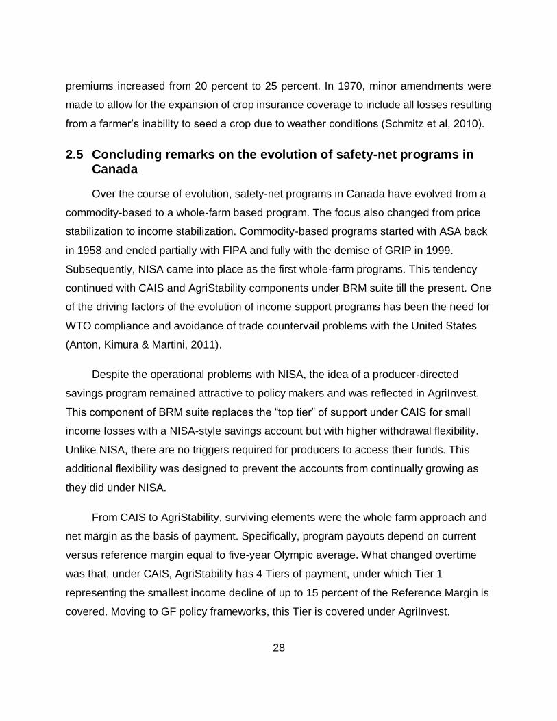
2.6 Ontario hog sector at a glance

Ontario has been the leading province in terms of hog numbers and farms

reporting hogs over censuses of agriculture from 2001 to 2016 (Fig.15 & Fig.16). Total

hog numbers in Ontario accounted for more than 30 percent of the hog numbers in

Canada (Fig.17).

Figure 15. Hog numbers by province from census 2001 to 2016 (x1,000)

Source: Statistics Canada. Table 32-10-0155-01: selected livestock and poultry, historical data

0

500

1,000

1,500

2,000

2,500

3,000

3,500

4,000

4,500

2001 2006 2011 2016

Num

ber

of hogs

Year

Ontario



Nova Scotia

New Brunswick

Quebec

Manitoba

Saskatchewan

Alberta

British Columbia

30

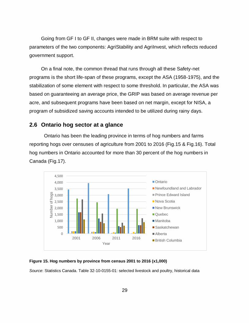
Figure 16. Hog farms by province - Census 2001 to 2016


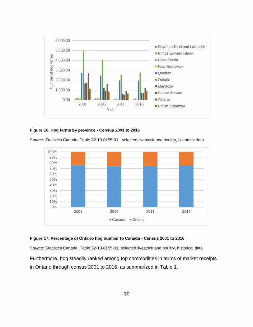
Figure 17. Percentage of Ontario hog number to Canada - Census 2001 to 2016


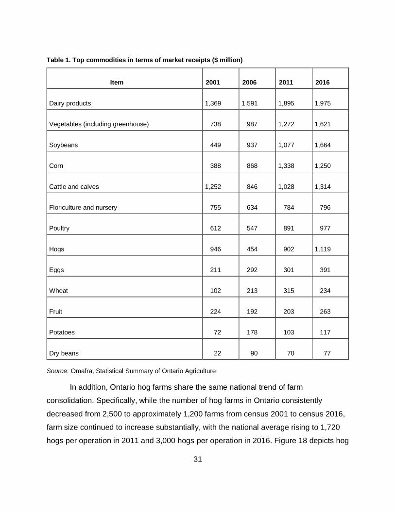
Furthermore, hog steadily ranked among top commodities in terms of market receipts

in Ontario through census 2001 to 2016, as summarized in Table 1.

0.00

1,000.00

2,000.00

3,000.00

4,000.00

5,000.00

6,000.00

2001 2006 2011 2016

Num

ber

of hog farm

s

Year



Nova Scotia

New Brunswick

Quebec

Ontario

Manitoba

Saskatchewan

Alberta

British Columbia

0%

10%

20%

30%

40%

50%

60%

70%

80%

90%

100%

2001 2006 2011 2016

Canada Ontario

31

Table 1. Top commodities in terms of market receipts ($ million)

Item 2001 2006 2011 2016

Dairy products 1,369 1,591 1,895 1,975

Vegetables (including greenhouse) 738 987 1,272 1,621

Soybeans 449 937 1,077 1,664

Corn 388 868 1,338 1,250

Cattle and calves 1,252 846 1,028 1,314

Floriculture and nursery 755 634 784 796

Poultry 612 547 891 977

Hogs 946 454 902 1,119

Eggs 211 292 301 391

Wheat 102 213 315 234

Fruit 224 192 203 263

Potatoes 72 178 103 117

Dry beans 22 90 70 77

Source: Omafra, Statistical Summary of Ontario Agriculture

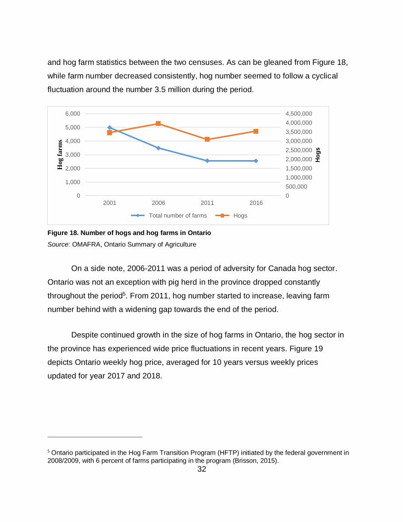
In addition, Ontario hog farms share the same national trend of farm

consolidation. Specifically, while the number of hog farms in Ontario consistently

decreased from 2,500 to approximately 1,200 farms from census 2001 to census 2016,

farm size continued to increase substantially, with the national average rising to 1,720

hogs per operation in 2011 and 3,000 hogs per operation in 2016. Figure 18 depicts hog

32

and hog farm statistics between the two censuses. As can be gleaned from Figure 18,

while farm number decreased consistently, hog number seemed to follow a cyclical

fluctuation around the number 3.5 million during the period.

Figure 18. Number of hogs and hog farms in Ontario

Source: OMAFRA, Ontario Summary of Agriculture

On a side note, 2006-2011 was a period of adversity for Canada hog sector.

Ontario was not an exception with pig herd in the province dropped constantly

throughout the period5. From 2011, hog number started to increase, leaving farm

number behind with a widening gap towards the end of the period.

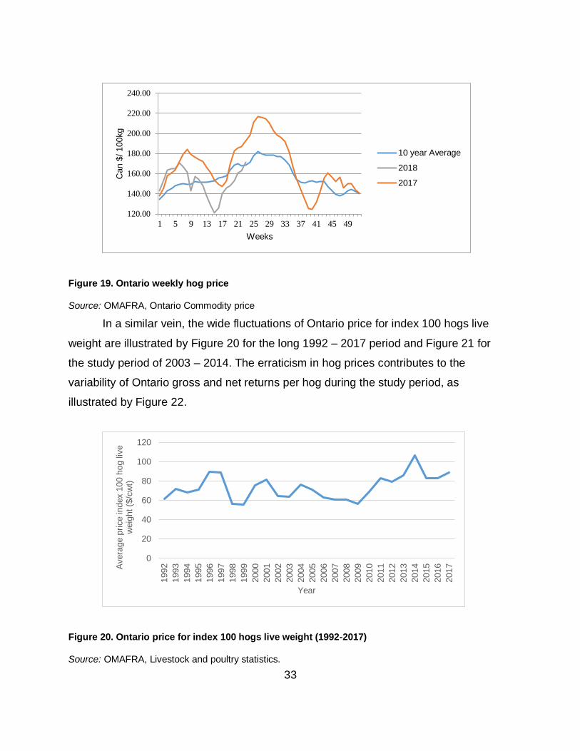
Despite continued growth in the size of hog farms in Ontario, the hog sector in

the province has experienced wide price fluctuations in recent years. Figure 19

depicts Ontario weekly hog price, averaged for 10 years versus weekly prices

updated for year 2017 and 2018.

5 Ontario participated in the Hog Farm Transition Program (HFTP) initiated by the federal government in

2008/2009, with 6 percent of farms participating in the program (Brisson, 2015).

0

500,000

1,000,000

1,500,000

2,000,000

2,500,000

3,000,000

3,500,000

4,000,000

4,500,000

0

1,000

2,000

3,000

4,000

5,000

6,000

2001 2006 2011 2016

Ho

gs

Hog

fa

rm

s

Total number of farms Hogs

33

Figure 19. Ontario weekly hog price

Source: OMAFRA, Ontario Commodity price

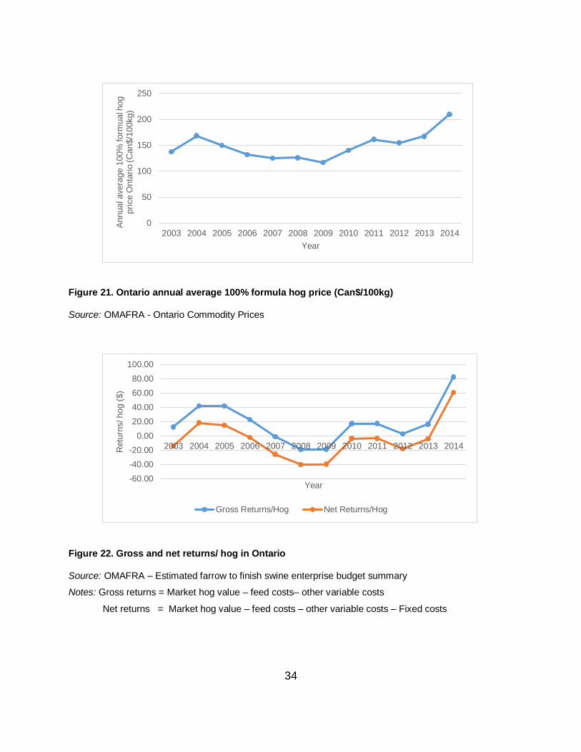
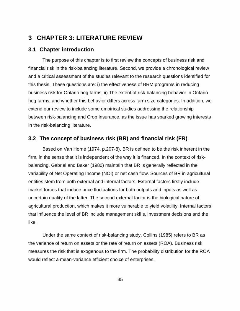
In a similar vein, the wide fluctuations of Ontario price for index 100 hogs live

weight are illustrated by Figure 20 for the long 1992 – 2017 period and Figure 21 for

the study period of 2003 – 2014. The erraticism in hog prices contributes to the

variability of Ontario gross and net returns per hog during the study period, as

illustrated by Figure 22.

Figure 20. Ontario price for index 100 hogs live weight (1992-2017)

Source: OMAFRA, Livestock and poultry statistics.

120.00

140.00

160.00

180.00

200.00

220.00

240.00

1 5 9 13 17 21 25 29 33 37 41 45 49

Can $

/ 100kg

Weeks

10 year Average

2018

2017

0

20

40

60

80

100

120

1992

1993

1994

1995

1996

1997

1998

1999

2000

2001

2002

2003

2004

2005

2006

2007

2008

2009

2010

2011

2012

2013

2014

2015

2016

2017Avera

ge p

rice index 1

00 h

og liv

e

weig

ht ($

/cw

t)

Year

34

Figure 21. Ontario annual average 100% formula hog price (Can$/100kg)

Source: OMAFRA - Ontario Commodity Prices

Figure 22. Gross and net returns/ hog in Ontario

Source: OMAFRA – Estimated farrow to finish swine enterprise budget summary

Notes: Gross returns = Market hog value – feed costs– other variable costs

Net returns = Market hog value – feed costs – other variable costs – Fixed costs

0

50

100

150

200

250

2003 2004 2005 2006 2007 2008 2009 2010 2011 2012 2013 2014

Annual avera

ge 1

00%

form

ual h

og

pri

ce O

nta

rio (C

an$/1

00kg)

Year

-60.00

-40.00

-20.00

0.00

20.00

40.00

60.00

80.00

100.00

2003 2004 2005 2006 2007 2008 2009 2010 2011 2012 2013 2014Retu

rns/ hog (

$)

Year

Gross Returns/Hog Net Returns/Hog

35

3 CHAPTER 3: LITERATURE REVIEW


The purpose of this chapter is to first review the concepts of business risk and

financial risk in the risk-balancing literature. Second, we provide a chronological review

and a critical assessment of the studies relevant to the research questions identified for

this thesis. These questions are: i) the effectiveness of BRM programs in reducing

business risk for Ontario hog farms; ii) The extent of risk-balancing behavior in Ontario

hog farms, and whether this behavior differs across farm size categories. In addition, we

extend our review to include some empirical studies addressing the relationship

between risk-balancing and Crop Insurance, as the issue has sparked growing interests

in the risk-balancing literature.

3.2 The concept of business risk (BR) and financial risk (FR)

Based on Van Horne (1974, p.207-8), BR is defined to be the risk inherent in the

firm, in the sense that it is independent of the way it is financed. In the context of risk-

balancing, Gabriel and Baker (1980) maintain that BR is generally reflected in the

variability of Net Operating Income (NOI) or net cash flow. Sources of BR in agricultural

entities stem from both external and internal factors. External factors firstly include

market forces that induce price fluctuations for both outputs and inputs as well as

uncertain quality of the latter. The second external factor is the biological nature of

agricultural production, which makes it more vulnerable to yield volatility. Internal factors

that influence the level of BR include management skills, investment decisions and the

like.

Under the same context of risk-balancing study, Collins (1985) refers to BR as

the variance of return on assets or the rate of return on assets (ROA). Business risk

measures the risk that is exogenous to the firm. The probability distribution for the ROA

would reflect a mean-variance efficient choice of enterprises.

36

With respect to financial risk, as mentioned by Barges (1963, p.16), FR is defined

to be the added variability of the net cash flows that results from the fixed financial

obligation associated with debt financing and cash leasing6. In this regard, FR can be

measured by firm’s leverage ratio. Also, Van Arsdell (1968) argued that financial risk

encompasses the risk of cash insolvency (p. 304).

According to Gabriel and Barker (1980), as BR can be reflected in the variability of

either net operating income or net cash flows, FR could also be defined in terms of net

operating income or net cash flow. The authors also maintain that in case FR is defined

in terms of net operating income, the fixed debt-servicing obligations would involve only

interest. In the other case, when FR is defined in terms of net cash flows, the fixed debt-

servicing obligations include both interest and principal.

On a further note, Collins (1985) contended that the leverage position chosen leads

to variations in the rate of returns of equity that is some multiple of BR. In this light, the

magnitude of this leverage multiplier may be regarded as FR.

The following sections provides a critical review of recent empirical studies relevant

to the research questions raised this thesis. Gaps in the literature and areas for future

research are also identified afterwards.

3.3 Review of recent studies related to the research questions

3.3.1 The extent of risk-balancing behavior

Escalante and Barry (2001) used optimization techniques in a simulation

framework to determine the extent of the risk-balancing strategy in reducing risk under an

integrated risk-management strategic approach. The authors employed the quadratic

programing model developed by Markowitz, which is equivalent to Freund’s formulation,

to derive the optimization framework for running the simulation. The objective of this

6 For the purpose of simplicity, only debt financing is considered in this study as the source of financial risk.

37

quadratic programing framework is maximizing expected utility of final wealth, i.e the

outcome variable. The paper concludes that risk-balancing, as a risk-management

strategy, has the potential to form synergistic relationships with other alternative

strategies. In this light, the greater appeal of a more diversified plan usually downplays

the risk-balancing strategy. A notable limitation of the paper lies in the simulation

approach itself. With this approach, results are challenging to validate and thus, should

be interpreted with caution.

Turvey and Kong (2009) employed theoretical model by Collins (1985) to

investigate the relationships between business risk and credit choices of 400 rural farm

households in China based on survey data in October 2007. Measure of risk-taking

attitude was also constructed from surveyed questions and incorporated into the model

as one of the controlling variables. The authors conducted 4 linear regression models

using Maximum Likelihood estimators. These regression models differ only in the

dependent variables, i.e., financial risk measures. They found evidence of risk balancing,

i.e., farmers facing higher production risks reduce financial risks with lower credit demand.

This evidence varied across financial risk measures. One limitation of this paper was the

employment of cross-sectional data, which failed to capture the dynamic relationship

between BR and credit risk decisions. Further, there was insufficient explanation for the

different results obtained from the 4 regressions.

Employing correlation coefficient between BR and FR as a measurement of risk-

balancing behavior, Escalante and Barry (2003) found evidence of risk-balancing for 80

farms in the United States from 1982 to1998. Using a similar approach, Ueza et al

(2014b) employed Pearson’s correlation coefficients between BR and FR as a measure

of risk-balancing for each farm. This coefficient was calculated over parings between one

year lagged BR and current year FR. As risk-balancing hypothesis maintains an inverse

relationship between BR and FR, the extent of risk-balancing is measured by the share

of farms with negative correlation coefficient. The authors argued that given the short time

series of the data (2003-2011), the statistical significance of the coefficients is less

38

relevant. They also concluded that the extent of risk balancing varied across farm size

categories and that larger farms for both beef and field crop farms showed evidenced of

risk-balancing of a larger degree compared to farms of smaller size categories.

The paper by De Mey et al (2014) used both correlation coefficient analysis and

regression approach to investigate risk-balancing hypothesis for EU-15 farm sector from

1995 to 2008. Findings were that 50 percent of farms showed evidence of strategic

adjustment of capital structure in response to a change in the level of BR. Nevertheless,

there was a lack of comparison and explanation about the different results obtained from

the two approaches employed in the research.

Wauters et al (2015) aims to theoretically introduce the novel framework of farm

household risk-balancing by extending the original risk-balancing framework of Gabriel

and Baker (1980) to household level. Based on this framework, farm households set a

constraint on the total household-level risk and balance farm and off-farm risks. The

authors derived equations linking farm activities, consumption and business and private

liquidity and argued that risk-balancing behaviour of farmers could be better understood

by considering risk at the household level. The framework showed that facing an

exegenous change in BR, risk-averse farm households may also respond by a change in

household buffering strategies, for instance, increasing their off-farm risk, and not only

by initiating a change in their financial position.

In general, the correlation coefficient analysis approach has its own limitation in

measuring the extent of risk-balancing as it fails to account for potential factors that could

influence financial risk decisions, for instance interests or the expected Net Operating

Income. This limitation can be overcome by using regression analysis.

3.3.2 The effectiveness of BRM program – How to measure business risk?

In a paper selected for presentation at Agricultural and Applied Economics

Association’s 2014 Annual Meeting, Minneapolis, Ueza et al assessed the impacts of

BRM program participation on farm BR across sectors, including beef, field crop, swine,

39

supply managed and others, by estimating the BR function using both Tobit and quantile

regression model (Ueza et al., 2014a). Downside risk, the dependent variable, was

measured as the percentage change in gross margin from previous year during the study

period from 2003 to 2011. Regression results showed that the coefficients for most

program participation states were negative and significant, suggesting that producers who

participate in one or more of the programs experienced smaller drops in gross margin

than producers who did not participate.

Also, these authors employed longitudinal data from 2003 to 2011 and compared the

distribution of BR with and without BRM/ AgriStability payments so as to examine the

effectiveness of BRM programs in reducing BR for Ontario beef and field crop farms

(Ueza et al., 2014b). The authors used two measures of BR, including the standard

deviation measure, i.e., standard deviation/ average income ratio, and the left-side semi-

kurtosis measure, i.e., the thickness measurement of the left tail of Net Operating Income.

While the former measure focuses on observations close to the mean, which represents

frequent small gains and losses, the latter emphasizes infrequent yet extreme losses.

They argued that the use of the left-side semi-kurtosis measure is more relevant as BRM/

AgriStability was aimed to provide coverage for large income decline. Findings were that

BRM/ AgriStability payments reduced BR for beef farms but not for field crop farms.

In a nutshell, downside risks were captured in both papers. Nevertheless, the way it

was measured was different across studies. Applying Tobit regression on downside risks

represented by the percentage change in gross margin, Ueza et al (2014a) were able to

segregate the drops from the gains in gross margin from previous year for estimating the

effects of BRM programs in reducing these drops. In this way of measurement, however,

the author cannot capture the downside variations of farms’ gross margin relative to its

central distribution, and thus fails to disentangle the extreme but infrequent losses in

farms’ gross margin from the small but frequent ones.

With reference to Ueza et al (2014b), employing the left-side semi-kurtosis to

represent BR, the authors were able to capture the magnitude of the extreme but

40

infrequent losses in net operating income of Ontario beef and field crop farms. However,

this measurement did not tell us if the distribution of net operating income was skewed

or not, and if it was skewed to the left of to the right. Put differently, it could not be

concluded from the study if downside BR outweighed upside BR, and from risk

management perspective, this should receive our attention. Another the limitation of the

study comes from the lack of Crop Insurance data, which is significant for field crop

farms. As such, one of the suggestions for future research is to incorporate Crop

Insurance data into analysis so as to deliver a better measurement of business risk.

3.3.3 Crop Insurance and risk-balancing behavior

Skees (1999) argued that “subsidized insurance will not take the risk out of

agriculture” (p. 35) as a result of risk-balancing behaviour. In particular, the author

maintained that as farmers regconize the value of crop insurance subsidies, the effects

on risk-taking behavior become counter-intuitive. Farmers with subsidized risk

management may push harder and faster and take on more risk. They will probably

borrow at higher rates as well, meaning they may “take on more and different risks until

their risk level returns to the pre-policy intervention level” (p. 36). The author

corroborated that when decision makers must pay for risk protection, the risk will be

internalized into the decision processes. When they pay less than they will get back in

indemnities resulting from insurance subsidies, society is paying people to take on

additional risk.

In this context of risk-balancing behavior, we would review some empirical

studies that set some ground for the question of whether Crop Insurance purchase

matters to the identification and measure of risk-balancing (Table 2). Specifically,

factors influencing Crop Insurance demand and the relationship between BRM/

AgriStability and Crop Insurance, i.e., they are substitutes or complements, were

explored in empirical studies to follow.

Sherrick et al (2004) investigated farmers’ decision to purchase Crop Insurance

and their choices among alternative products. The authors used a two-stage estimation

procedure that considers the decision to purchase or not, and then evaluated the choice

41

among alternate Crop Insurance products in cases of use. A survey of farmers in

Illinois, Indiana, and Iowa provided the data for the analysis. Factors included in the

model were the level of BR, risk management options, debt use (FR), risk attitude,

tenure, age and education of farm operator, expected yields, farm size, livestock

enterprises, and off-farm income. Producers facing greater levels of business risk are

expected to have a stronger demand for Crop Insurance and use more comprehensive

insurance products. The paper concluded that farmers who are more highly leveraged,

less wealthy, riskier, and operate larger acreages engage more extensively in insurance

and are more likely to choose revenue protection versus more specific yield and hail

protection insurance. The pattern of results found in this study needs to be tested in

other agricultural regions to verify the extent of their applicability.

Given from the previous section review that BRM programs are effective in

reducing farm BR along with the conclusion from this study on a significant positive

relationship between BR and CI demand, can it be inferred that BRM programs reduce

farmers’ incentive to purchase CI? Further empirical analysis would be needed to

address this research question.

On account of risk-balancing evidence as revealed from previous empirical

studies, which suggest an inverse relationship between BR and FR, the regression

model in this paper may exhibit multicollinearity with BR and FR both entering the model

as explanatory variables.

Cabas et al (2008) explored determinants of farmers’ participation in Crop

Insurance schemes, with participation being decomposed into entry and exit decisions.

The study employed data on Ontario soybean crop insurance plan, covering the 1988-

2004 period for 8 counties in southern Ontario: Chatham-Kent, Elgin, Essex,

Haldimand-Norfolk, Huron, Lambton, Middlesex and Perth. Explanatory variables

affecting Crop Insurance participation included: premium rate, soybean price, variance

of the expected soybean price, yield, variance of county yield, number of farmers

qualifying for insurance payout in the preceding year and proportion of total acreage

devoted to soybeans at the county level. The study concluded that price variables were

particularly important for farmers considering enrolling in crop insurance, while yield

42

variables and other risk management opportunities were more important for farmers

who have been in the program but are deciding to exit.

Iff et al (2015) used data from the nationally representative Agricultural Resource

Management Survey to consider how Federal Crop Insurance (FCI) program influences

various measures of farm debt use. Findings were that FCI participation was associated

with an increase in the use of short-term debt, but not long-term debt. This finding is

consistent with risk-balancing behavior and current trend in the farm sector. Besides,

the study by Escalante and Barry (2003) looked at the determinants of FR based on

Collins (1985). Independent variables included amount of Crop Insurance coverage,

farm tenure position and crop diversification. The results revealed that risk-balancing

was compatible with crop diversification and insurance protection plans.

Given the compatibility between risk balancing and alternative strategies

demonstrated in this study, the findings set good ground and provide motivation for

investigating the extent of risk reduction realized under a more integrated risk

management approach that takes into account Crop Insurance purchase. Some

pending questions may arise from the above studies: Is Crop Insurance an alternative

strategy to BRM payments? And as such, do BRM programs reduce farmers’ incentives

to purchase Crop Insurance?

Also, the paper by Ueza et al (2014a) investigated the interrelated dynamics of

participation in Crop Insurance, AgriStability and AgriInvest programs. It was concluded

that programs tend to be used together rather than independently: the pairwise

correlations between the residuals in the multivariate model are positive and significant,

with the correlation between participation in Crop Insurance and AgriStability being the

strongest. With respect to risk-reducing effects, Crop Insurance did not seem to be able

to mitigate downside risk when used independently, but delivered a great effect when

jointly used with AgriStability. On account of the author’s argument that two programs

are complementary if they mitigate downside risk more when used jointly than when

either program is used in isolation, Crop Insurance and AgriStability are complements

rather than substitutes.

43

3.4 Chapter summary

The above review highlights a number of gaps in the existing literature. The

purpose of this thesis is to bridge some of these gaps. First, while relevant papers had

different ways to measure the downside risks of Ontario grain and beef farms, little

evidence has been found for the hog sector in the province. More importantly, little

evidence has been found on a conclusive way of measuring downside risk that could

capture the magnitude of infrequent but extreme losses while accounting for the

skewness property of its distribution. In addition, due to data constraint, Crop Insurance

data was not incorporated into calculation of business risk in the previous studies.

Secondly, while a number of paper used pairwise correlation coefficient to

measure the extent of risk-balancing in agricultural sectors in Canada, some other

studies employed regression analysis to account for other factors that may also have an

impact on financial risk decisions. In addition, whether this extent differs among farms

of different size class categories and/ or across agricultural sectors has not been fully

investigated.

Last but not the least, while BRM/ AgriStability and Crop Insurance were proved

to be complements in reducing business risk for farms in a previous study by Ueza et al

(2014a), whether participation in these programs substitutes or complements each other

opens up an area for further research. In addition, the paper by Cabas et al (2008)

suggested a novel way of looking at the demand for Crop Insurance decomposed

between entry and exit decisions. Altogether, an inspiring question has arisen on the

impacts of BRM/ AgriStability payments on Crop Insurance new enrolment and exit

decisions.

A summary of selected empirical studies relevant to the research questions

identified in this thesis is provided in Table 2.

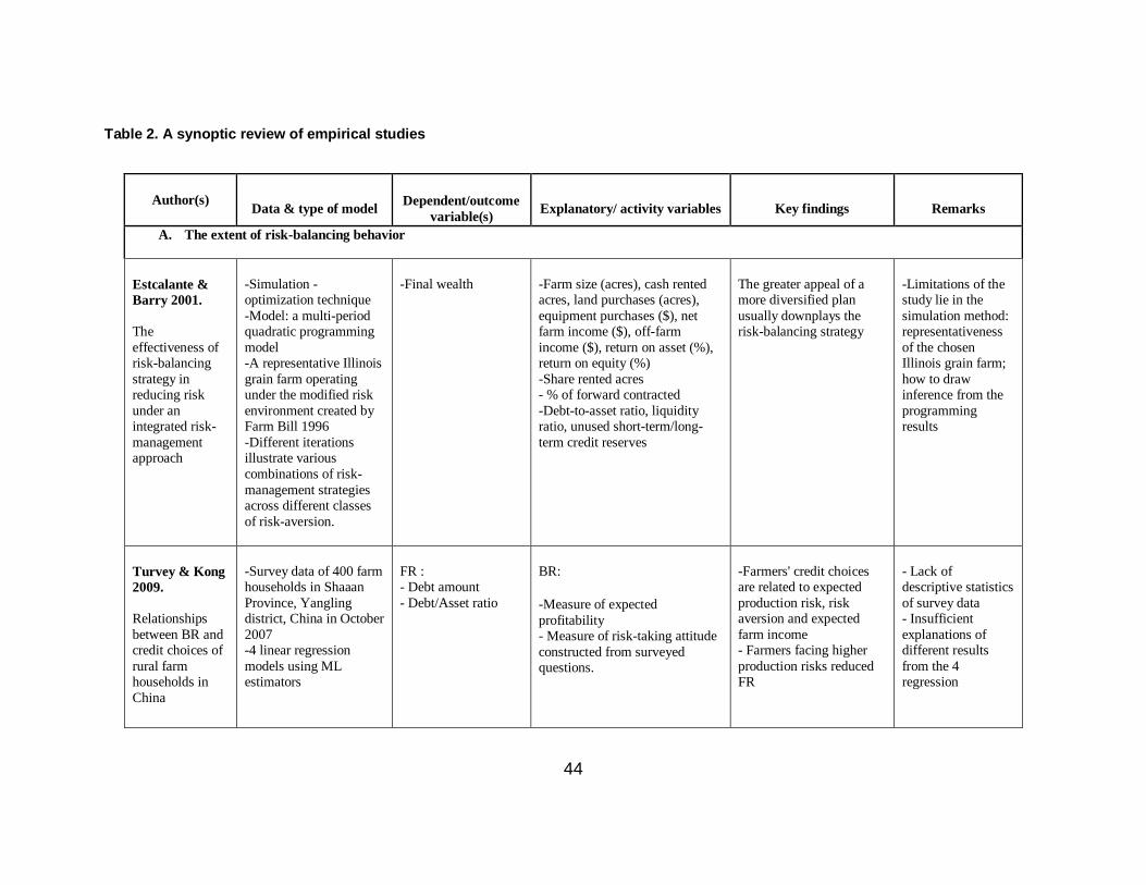
44

Table 2. A synoptic review of empirical studies

Author(s) Data & type of model

Dependent/outcome

variable(s) Explanatory/ activity variables Key findings Remarks

A. The extent of risk-balancing behavior

Estcalante &

Barry 2001.

The

effectiveness of risk-balancing

strategy in reducing risk

under an integrated risk-

management approach

-Simulation - optimization technique

-Model: a multi-period quadratic programming

model -A representative Illinois

grain farm operating under the modified risk

environment created by Farm Bill 1996

-Different iterations illustrate various

combinations of risk-

management strategies across different classes

of risk-aversion.

-Final wealth -Farm size (acres), cash rented acres, land purchases (acres),

equipment purchases ($), net farm income ($), off-farm

income ($), return on asset (%), return on equity (%)

-Share rented acres - % of forward contracted

-Debt-to-asset ratio, liquidity ratio, unused short-term/long-

term credit reserves

The greater appeal of a more diversified plan

usually downplays the risk-balancing strategy

-Limitations of the study lie in the

simulation method: representativeness

of the chosen Illinois grain farm;

how to draw inference from the

programming results

Turvey & Kong

2009. Relationships

between BR and credit choices of

rural farm households in

China

-Survey data of 400 farm households in Shaaan

Province, Yangling district, China in October

2007 -4 linear regression

models using ML estimators

FR : - Debt amount

- Debt/Asset ratio

BR:

-Measure of expected

profitability - Measure of risk-taking attitude

constructed from surveyed questions.

-Farmers' credit choices are related to expected

production risk, risk aversion and expected

farm income - Farmers facing higher

production risks reduced FR

- Lack of descriptive statistics

of survey data - Insufficient

explanations of different results

from the 4 regression

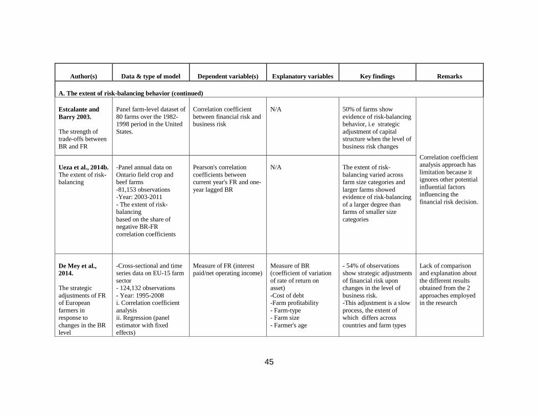
45

Author(s) Data & type of model Dependent variable(s) Explanatory variables Key findings Remarks

A. The extent of risk-balancing behavior (continued)

Estcalante and

Barry 2003.

The strength of trade-offs between

BR and FR

Panel farm-level dataset of

80 farms over the 1982-1998 period in the United

States.

Correlation coefficient

between financial risk and business risk

N/A 50% of farms show

evidence of risk-balancing behavior, i.e strategic

adjustment of capital structure when the level of

business risk changes

Correlation coefficient analysis approach has

limitation because it ignores other potential

influential factors influencing the

financial risk decision.

Ueza et al., 2014b. The extent of risk-balancing

-Panel annual data on

Ontario field crop and beef farms

-81,153 observations -Year: 2003-2011

- The extent of risk-balancing

based on the share of negative BR-FR

correlation coefficients

Pearson's correlation

coefficients between current year's FR and one-

year lagged BR

N/A The extent of risk-

balancing varied across farm size categories and

larger farms showed evidence of risk-balancing

of a larger degree than farms of smaller size

categories

De Mey et al.,

2014. The strategic

adjustments of FR of European

farmers in response to

changes in the BR level

-Cross-sectional and time series data on EU-15 farm

sector - 124,132 observations

- Year: 1995-2008 i. Correlation coefficient

analysis ii. Regression (panel

estimator with fixed effects)

Measure of FR (interest paid/net operating income)

Measure of BR (coefficient of variation

of rate of return on asset)

-Cost of debt -Farm profitability

- Farm-type - Farm size

- Farmer's age

- 54% of observations show strategic adjustments

of financial risk upon changes in the level of

business risk. -This adjustment is a slow

process, the extent of which differs across

countries and farm types

Lack of comparison and explanation about

the different results obtained from the 2

approaches employed in the research

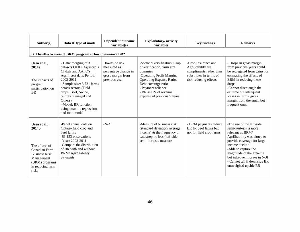
46

Author(s) Data & type of model Dependent/outcome

variable(s)

Explanatory/ activity

variables Key findings Remarks

B. The effectiveness of BRM program - How to measure BR?

Ueza et al.,

2014a

The impacts of program

participation on BR

- Data: merging of 3 datasets OFID, Agricorp’s

CI data and AAFC’s

AgriInvest data. Period: 2003-2011

'-Sample size: 8,721 farms across sectors (Field

crops, Beef, Swine, Supply managed and

Others) '-Model: BR function

using quantile regression and tobit model

Downside risk measured as

percentage change in

gross margin from previous year

-Sector diversification, Crop diversification, farm size

dummies

-Operating Profit Margin, Operating Expense Ratio,

Debt coverage ratio - Payment reliance

- BR as CV of revenue/ expense of previous 5 years

-Crop Insurance and AgriStability are

compliments rather than

substitutes in terms of risk-reducing effects

- Drops in gross margin from previous years could

be segregated from gains for

estimating the effects of BRM in reducing these

drops -Cannot disentangle the

extreme but infrequent losses in farms' gross

margin from the small but frequent ones

Ueza et al.,

2014b

The effects of

Canadian Farm Business Risk

Management (BRM) programs

in reducing farm risks

-Panel annual data on Ontario field crop and

beef farms -81,153 observations

-Year: 2003-2011 -Compare the distribution

of BR with and without BRM/ AgriStability

payments

-N/A -Measure of business risk (standard deviation/ average

income) & the frequency of catastrophic loss (left-side

semi-kurtosis measure

- BRM payments reduce BR for beef farms but

not for field crop farms

-The use of the left-side semi-kurtosis is more

relevant as BRM/ AgriStability was aimed to

provide coverage for large income decline

-Able to capture the magnitude of the extreme

but infrequent losses in NOI - Cannot tell if downside BR

outweighed upside BR

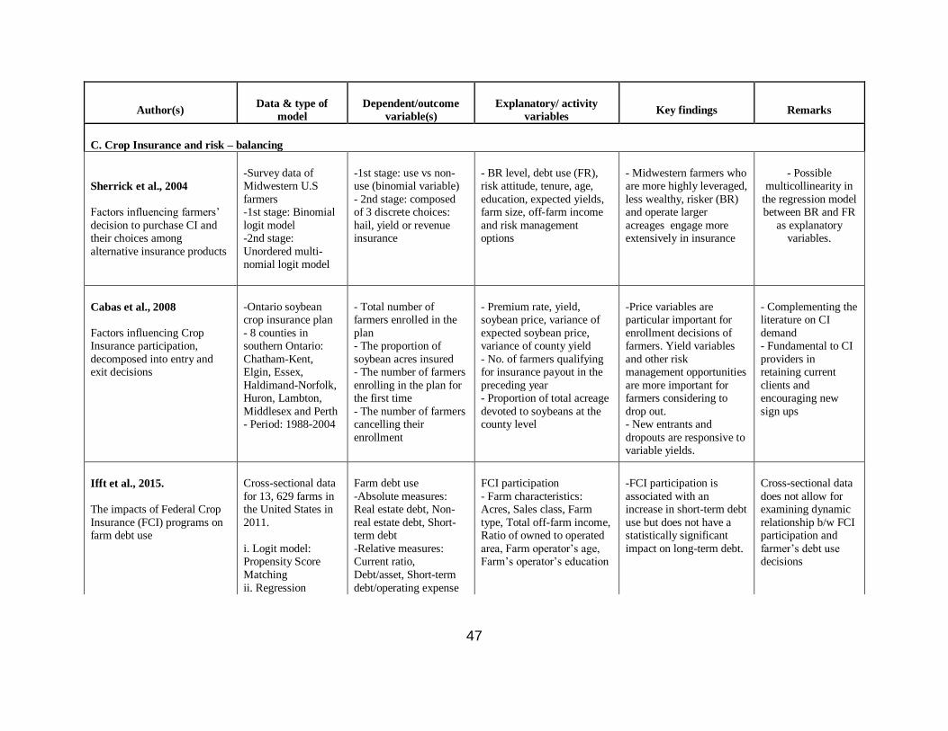
47

Author(s) Data & type of

model

Dependent/outcome

variable(s)



C. Crop Insurance and risk – balancing

Sherrick et al., 2004 Factors influencing farmers’

decision to purchase CI and their choices among

alternative insurance products

-Survey data of Midwestern U.S

farmers -1st stage: Binomial

logit model -2nd stage:

Unordered multi-nomial logit model

-1st stage: use vs non-use (binomial variable)

- 2nd stage: composed of 3 discrete choices:

hail, yield or revenue insurance

- BR level, debt use (FR), risk attitude, tenure, age,

education, expected yields, farm size, off-farm income

and risk management options

- Midwestern farmers who are more highly leveraged,

less wealthy, risker (BR) and operate larger

acreages engage more extensively in insurance

- Possible multicollinearity in

the regression model between BR and FR

as explanatory variables.

Cabas et al., 2008

Factors influencing Crop Insurance participation,

decomposed into entry and exit decisions

-Ontario soybean crop insurance plan

- 8 counties in southern Ontario:

Chatham-Kent, Elgin, Essex,

Haldimand-Norfolk, Huron, Lambton,

Middlesex and Perth - Period: 1988-2004

- Total number of farmers enrolled in the

plan - The proportion of

soybean acres insured - The number of farmers

enrolling in the plan for the first time

- The number of farmers cancelling their

enrollment

- Premium rate, yield, soybean price, variance of

expected soybean price, variance of county yield

- No. of farmers qualifying for insurance payout in the

preceding year - Proportion of total acreage

devoted to soybeans at the county level

-Price variables are particular important for

enrollment decisions of farmers. Yield variables

and other risk management opportunities

are more important for farmers considering to

drop out. - New entrants and

dropouts are responsive to variable yields.

- Complementing the literature on CI

demand - Fundamental to CI

providers in retaining current

clients and encouraging new

sign ups

Ifft et al., 2015. The impacts of Federal Crop

Insurance (FCI) programs on farm debt use

Cross-sectional data

for 13, 629 farms in the United States in

2011.

i. Logit model: Propensity Score

Matching

ii. Regression

Farm debt use

-Absolute measures: Real estate debt, Non-

real estate debt, Short-term debt

-Relative measures: Current ratio,

Debt/asset, Short-term

debt/operating expense

FCI participation

- Farm characteristics: Acres, Sales class, Farm

type, Total off-farm income, Ratio of owned to operated

area, Farm operator’s age, Farm’s operator’s education

-FCI participation is

associated with an increase in short-term debt

use but does not have a statistically significant

impact on long-term debt.

Cross-sectional data

does not allow for examining dynamic

relationship b/w FCI participation and

farmer’s debt use decisions

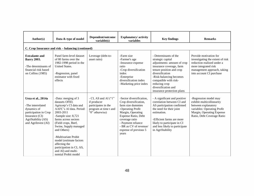
48

Author(s) Data & type of model Dependent/outcome

variable(s)



C. Crop Insurance and risk – balancing (continued)

Estcalante and

Barry 2003.

-The determinants of financial risk based

on Collins (1985)

Panel farm-level dataset

of 80 farms over the 1982-1998 period in the

United States.

-Regression, panel estimator with fixed

effects

Leverage (debt-to-

asset ratio)

-Farm size

-Farmer's age -Insurance expense

ratio -Crop diversification

index -Enterprise

diversification index -Marketing price index

- Determinants of the

strategic capital adjustments: amount of crop

insurance coverage, farm tenure position and crop

diversification -Risk-balancing becomes

compatible with risk-reducing crop

diversification and insurance protection plans

Provide motivation for

investigating the extent of risk reduction realized under a

more integrated risk management approach, taking

into account CI purchase

Ueza et al., 2014a -The interrelated

dynamics of participation in Crop

Insurance (CI) AgriStability (AS)

and AgriInvest (AI)

-Data: merging of 3

datasets OFID, Agricorp’s CI data and

AAFC’s AI data. Period: 2003-2011

-Sample size: 8,721 farms across sectors

(Field crops, Beef, Swine, Supply managed

and Others)

-Multivariate Probit model (estimate factors

affecting the participation in CI, AS,

and AI) and multi-nomial Probit model

- CI, AS and AI (“1”

if producer participates in the

program at time t and “0” otherwise)

-Sector diversification,

Crop diversification, farm size dummies

-Operating Profit Margin, Operating

Expense Ratio, Debt coverage ratio

- Payment reliance - BR as CV of revenue/

expense of previous 5 years

- A significant and positive

correlation between CI and AS participation confirmed

the need for their joint estimation.

-Efficient farms are more

likely to participate in CI and less likely to participate

in AgriStability

-Regression model may

exhibit multicollinearity between explanatory

variables: Operating Profit Margin, Operating Expense

Ratio, Debt Coverage Ratio

49

4 CHAPTER 4: ANALYTICAL FRAMEWORK


This chapter develops the theoretical model for this study. The first section relies

heavily on the conceptual frameworks of risk-balancing introduced by Gabriel and Baker

(1980) and later by Collins (1985) to bring out the key analytical issues and the basic

relationships among the variables. In section two, the model by Collins (1985) is

augmented by incorporating Crop Insurance into it. The augmented model is used to

develop the comparative statistic results, which will guide the empirical analysis of this

study.

4.2 Theoretical literature of risk-balancing

The total risk faced by a business entity can be considered as a sum of business

risk, i.e., risk directly associated with operating the business and financial risk, i.e., risk

associated with financial dealings of the business entity. In this sense, financial risk may

not be directly linked to the day-to-day business operations.

Gabriel and Baker (1980) developed a conceptual model that links production,

investment and financing decisions via a risk constraint. In their model, it is assumed

that “the decision maker has identified both firm survival and profit maximization as

goals, where firm survival is of primary importance” (p. 561). The decision maker

maximizes net returns subject to the constraint that total risk does not exceed the

maximum tolerable level.

Defined as the added variability of the net cash flows owing to the fixed financial

obligations associated with debt financing and cash leasing7, financial risk is formulated

as follows:

7 For the purpose of simplicity, only debt financing will be referred to as a source of financial risk in Gabriel

and Barker (1980).

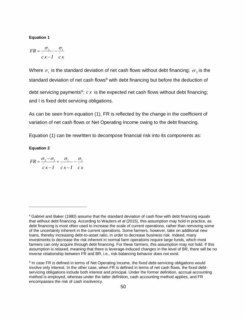
50

Equation 1

2 1FR

c x I c x

Where 1 is the standard deviation of net cash flows without debt financing; 2 is the

standard deviation of net cash flows8 with debt financing but before the deduction of

debt servicing payments9; c x

is the expected net cash flows without debt financing;

and I is fixed debt servicing obligations.

As can be seen from equation (1), FR is reflected by the change in the coefficient of

variation of net cash flows or Net Operating Income owing to the debt financing.

Equation (1) can be rewritten to decompose financial risk into its components as:

Equation 2

2 1 1 1FR

c x I c x I c x

8 Gabriel and Baker (1980) assume that the standard deviation of cash flow with debt financing equals that without debt financing. According to Wauters et al (2015), this assumption may hold in practice, as debt financing is most often used to increase the scale of current operations, rather than removing some of the uncertainty inherent in the current operations. Some farmers, however, take on additional new loans, thereby increasing debt-to-asset ratio, in order to decrease business risk. Indeed, many investments to decrease the risk inherent in normal farm operations require large funds, which most farmers can only acquire through debt financing. For these farmers, this assumption may not hold. If this assumption is relaxed, meaning that there is leverage-induced changes in the level of BR, there will be no inverse relationship between FR and BR, i.e., risk-balancing behavior does not exist. 9 In case FR is defined in terms of Net Operating Income, the fixed debt-servicing obligations would involve only interest. In the other case, when FR is defined in terms of net cash flows, the fixed debt-servicing obligations include both interest and principal. Under the former definition, accrual accounting method is employed, whereas under the latter definition, cash accounting method applies, and FR encompasses the risk of cash insolvency.

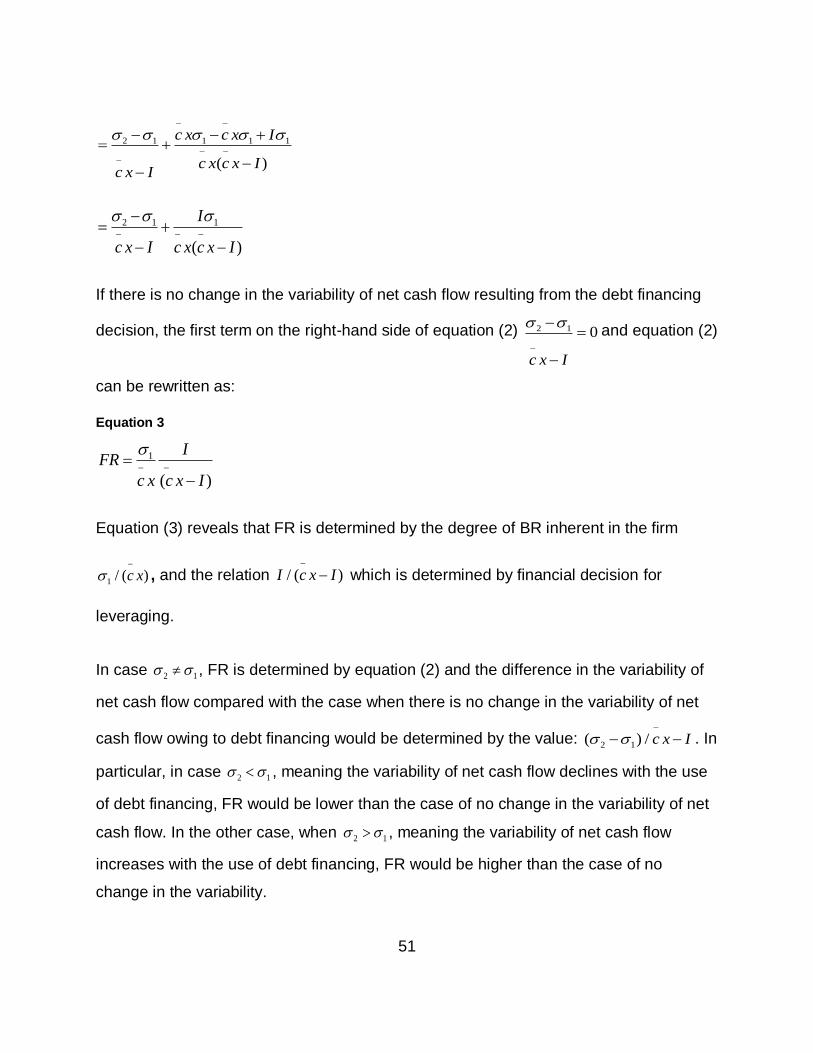
51

2 1 1 1 1

( )

c x c x I

c x c x Ic x I

2 1 1

( )

I

c x I c x c x I

If there is no change in the variability of net cash flow resulting from the debt financing

decision, the first term on the right-hand side of equation (2) 2 1 0

c x I

and equation (2)

can be rewritten as:

Equation 3

1

( )

IFR

c x c x I

Equation (3) reveals that FR is determined by the degree of BR inherent in the firm

1 / ( )c x

, and the relation / ( )I c x I

which is determined by financial decision for

leveraging.

In case 2 1 , FR is determined by equation (2) and the difference in the variability of

net cash flow compared with the case when there is no change in the variability of net

cash flow owing to debt financing would be determined by the value: 2 1( ) / c x I

. In

particular, in case 2 1 , meaning the variability of net cash flow declines with the use

of debt financing, FR would be lower than the case of no change in the variability of net

cash flow. In the other case, when 2 1 , meaning the variability of net cash flow

increases with the use of debt financing, FR would be higher than the case of no

change in the variability.

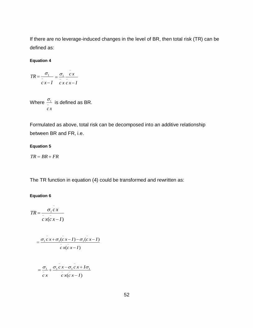
52

If there are no leverage-induced changes in the level of BR, then total risk (TR) can be

defined as:

Equation 4

1TR

c x I

1 c x

c x c x I

Where 1

c x

is defined as BR.

Formulated as above, total risk can be decomposed into an additive relationship

between BR and FR, i.e.

Equation 5

TR BR FR

The TR function in equation (4) could be transformed and rewritten as:

Equation 6

1

( )

c xTR

c x c x I

1 1 1( ) ( )

( )

c x c x I c x I

c x c x I

1 1 1 1

( )

c x c x I

c x c x c x I

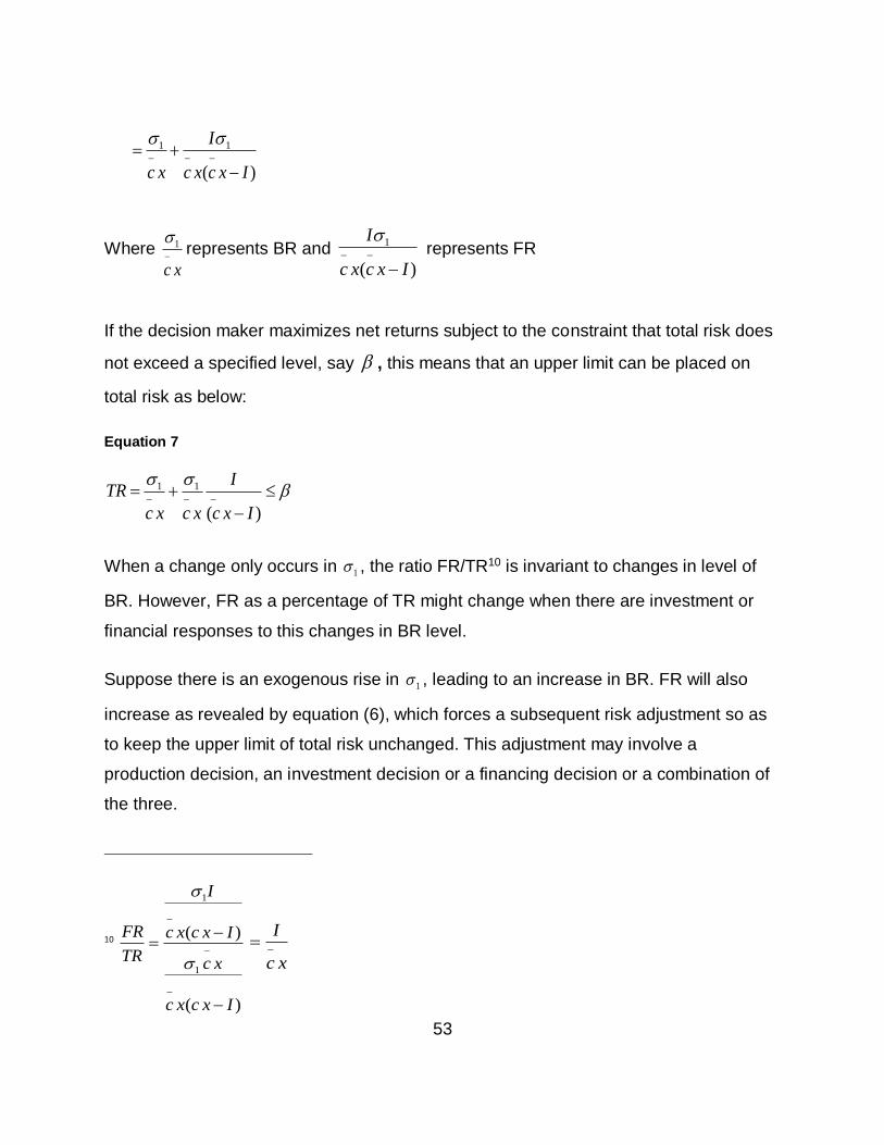
53

1 1

( )

I

c x c x c x I

Where 1

c x

represents BR and 1

( )

I

c x c x I

represents FR

If the decision maker maximizes net returns subject to the constraint that total risk does

not exceed a specified level, say , this means that an upper limit can be placed on

total risk as below:

Equation 7

1 1

( )

ITR

c x c x c x I

When a change only occurs in 1 , the ratio FR/TR10 is invariant to changes in level of

BR. However, FR as a percentage of TR might change when there are investment or

financial responses to this changes in BR level.

Suppose there is an exogenous rise in 1 , leading to an increase in BR. FR will also

increase as revealed by equation (6), which forces a subsequent risk adjustment so as

to keep the upper limit of total risk unchanged. This adjustment may involve a

production decision, an investment decision or a financing decision or a combination of

the three.

10

1

1

( )

( )

I

FR c x c x I

TR c x

c x c x I

I

c x

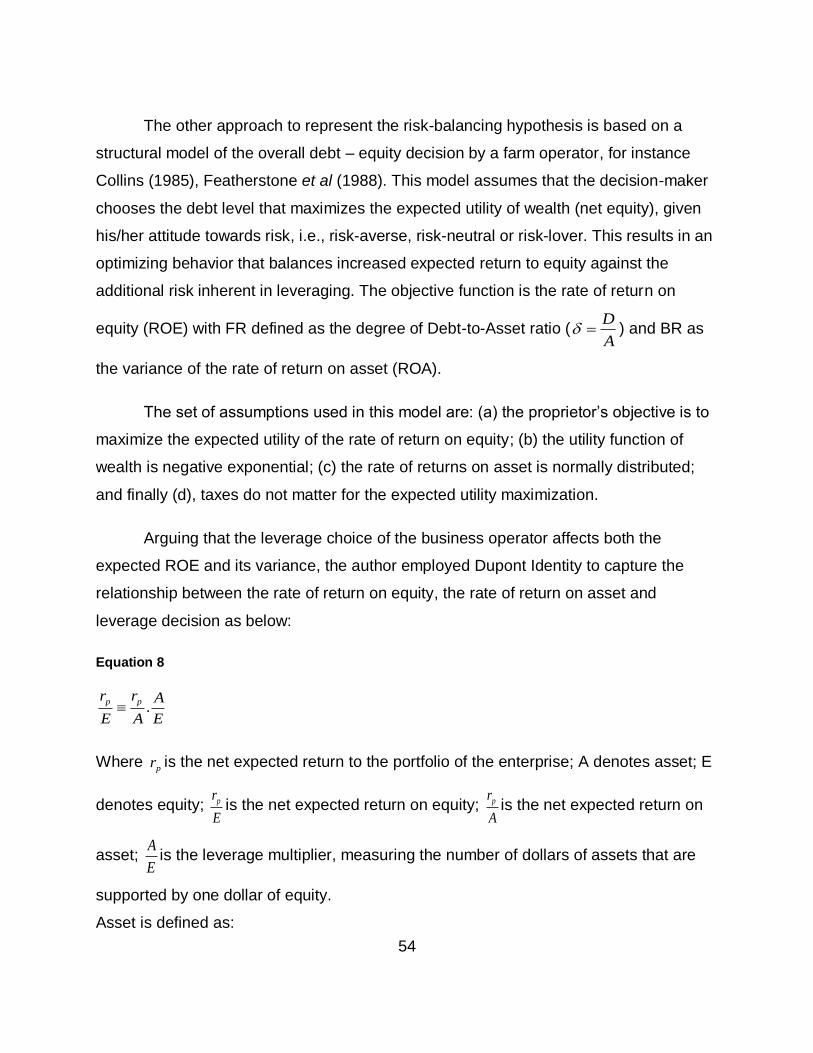
54

The other approach to represent the risk-balancing hypothesis is based on a

structural model of the overall debt – equity decision by a farm operator, for instance

Collins (1985), Featherstone et al (1988). This model assumes that the decision-maker

chooses the debt level that maximizes the expected utility of wealth (net equity), given

his/her attitude towards risk, i.e., risk-averse, risk-neutral or risk-lover. This results in an

optimizing behavior that balances increased expected return to equity against the

additional risk inherent in leveraging. The objective function is the rate of return on

equity (ROE) with FR defined as the degree of Debt-to-Asset ratio (D

A ) and BR as

the variance of the rate of return on asset (ROA).

The set of assumptions used in this model are: (a) the proprietor’s objective is to

maximize the expected utility of the rate of return on equity; (b) the utility function of

wealth is negative exponential; (c) the rate of returns on asset is normally distributed;

and finally (d), taxes do not matter for the expected utility maximization.

Arguing that the leverage choice of the business operator affects both the

expected ROE and its variance, the author employed Dupont Identity to capture the

relationship between the rate of return on equity, the rate of return on asset and

leverage decision as below:

Equation 8

.p pr r A

E A E

Where pr is the net expected return to the portfolio of the enterprise; A denotes asset; E

denotes equity; pr

Eis the net expected return on equity; pr

Ais the net expected return on

asset; A

Eis the leverage multiplier, measuring the number of dollars of assets that are

supported by one dollar of equity.

Asset is defined as:

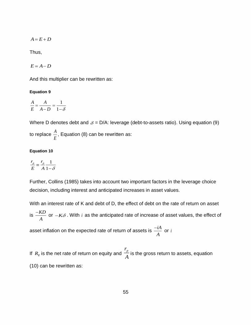
55

A E D

Thus,

E A D

And this multiplier can be rewritten as:

Equation 9

A A

E A D

1

1

Where D denotes debt and = D/A: leverage (debt-to-assets ratio). Using equation (9)

to replace A

E, Equation (8) can be rewritten as:

Equation 10

1

1

p pr r

E A

Further, Collins (1985) takes into account two important factors in the leverage choice

decision, including interest and anticipated increases in asset values.

With an interest rate of K and debt of D, the effect of debt on the rate of return on asset

is KD

A

or K . With i as the anticipated rate of increase of asset values, the effect of

asset inflation on the expected rate of return of assets is iA

A

or i

If ER is the net rate of return on equity and pr

Ais the gross return to assets, equation

(10) can be rewritten as:

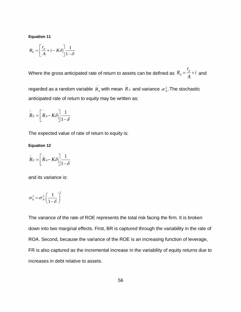
56

Equation 11

1

1

p

E

rR i K

A

Where the gross anticipated rate of return to assets can be defined as p

A

rR i

A and

regarded as a random variable ~

AR with mean AR

and variance 2

A .The stochastic

anticipated rate of return to equity may be written as:

1

1E AR R K

The expected value of rate of return to equity is:

Equation 12

1

1E AR R K

and its variance is:

2

2 2 1.

1E A

The variance of the rate of ROE represents the total risk facing the firm. It is broken

down into two marginal effects. First, BR is captured through the variability in the rate of

ROA. Second, because the variance of the ROE is an increasing function of leverage,

FR is also captured as the incremental increase in the variability of equity returns due to

increases in debt relative to assets.

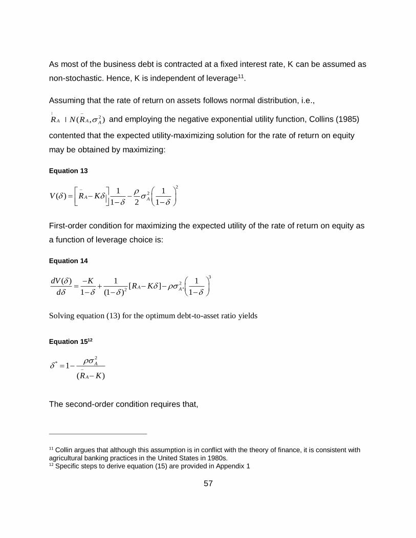
57

As most of the business debt is contracted at a fixed interest rate, K can be assumed as

non-stochastic. Hence, K is independent of leverage11.

Assuming that the rate of return on assets follows normal distribution, i.e.,

2( , )A A AR N R

and employing the negative exponential utility function, Collins (1985)

contented that the expected utility-maximizing solution for the rate of return on equity

may be obtained by maximizing:

Equation 13

2

21 1( )

1 2 1A AV R K

First-order condition for maximizing the expected utility of the rate of return on equity as

a function of leverage choice is:

Equation 14

3

2

2

( ) 1 1[ ] .

1 (1 ) 1A A

dV KR K

d

Solving equation (13) for the optimum debt-to-asset ratio yields

Equation 1512

2* 1

( )

A

AR K

The second-order condition requires that,

11 Collin argues that although this assumption is in conflict with the theory of finance, it is consistent with

agricultural banking practices in the United States in 1980s. 12 Specific steps to derive equation (15) are provided in Appendix 1

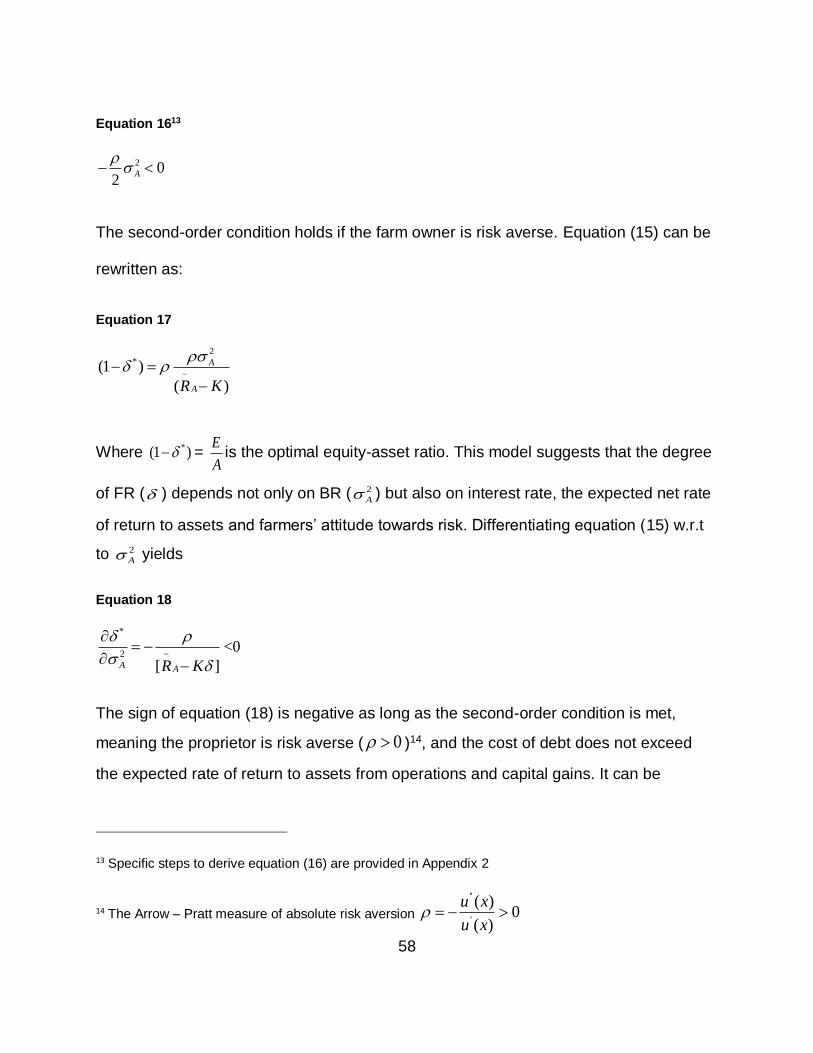
58

Equation 1613

2 02

A

The second-order condition holds if the farm owner is risk averse. Equation (15) can be

rewritten as:

Equation 17

2*(1 )

( )

A

AR K

Where *(1 ) = E

Ais the optimal equity-asset ratio. This model suggests that the degree

of FR ( ) depends not only on BR ( 2

A ) but also on interest rate, the expected net rate

of return to assets and farmers’ attitude towards risk. Differentiating equation (15) w.r.t

to 2

A yields

Equation 18

*

2

[ ]A AR K

<0

The sign of equation (18) is negative as long as the second-order condition is met,

meaning the proprietor is risk averse ( 0 )14, and the cost of debt does not exceed

the expected rate of return to assets from operations and capital gains. It can be

13 Specific steps to derive equation (16) are provided in Appendix 2

14 The Arrow – Pratt measure of absolute risk aversion

''

'

( )0

( )

u x

u x

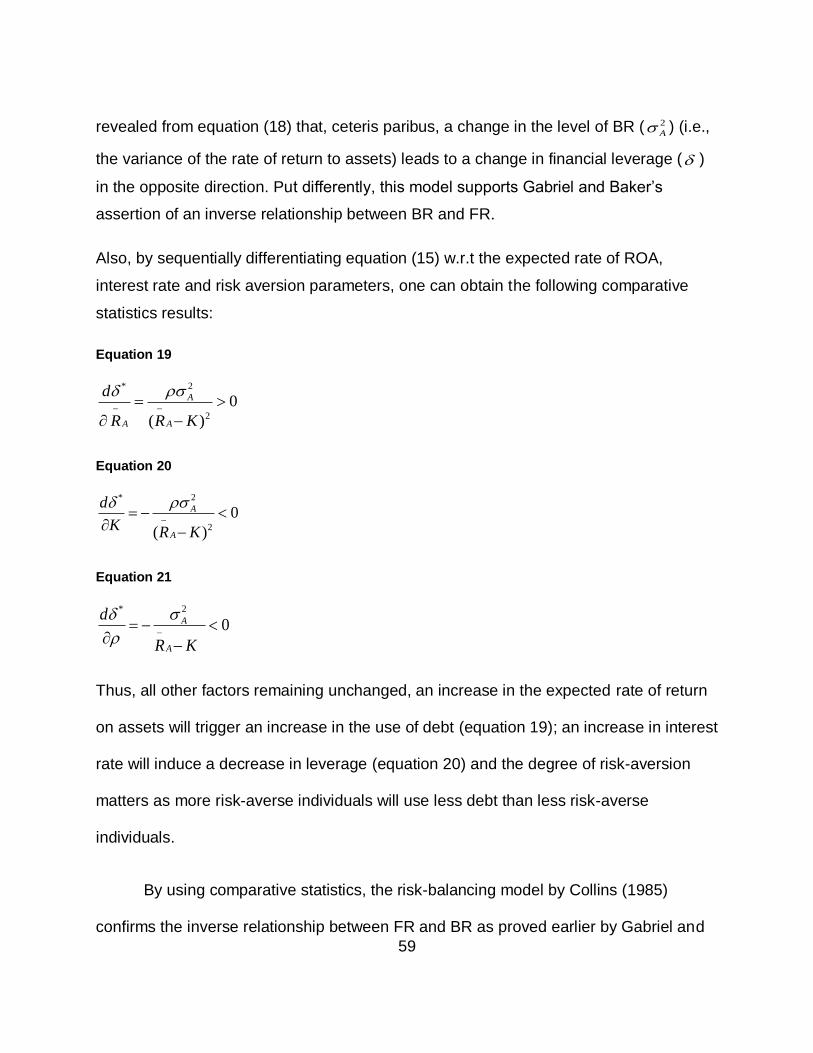
59

revealed from equation (18) that, ceteris paribus, a change in the level of BR ( 2

A ) (i.e.,

the variance of the rate of return to assets) leads to a change in financial leverage ( )

in the opposite direction. Put differently, this model supports Gabriel and Baker’s

assertion of an inverse relationship between BR and FR.

Also, by sequentially differentiating equation (15) w.r.t the expected rate of ROA,

interest rate and risk aversion parameters, one can obtain the following comparative

statistics results:

Equation 19

2*

2

0

( )

A

A A

d

R R K

Equation 20

2*

2

0

( )

A

A

d

K R K

Equation 21

2*

0A

A

d

R K

Thus, all other factors remaining unchanged, an increase in the expected rate of return

on assets will trigger an increase in the use of debt (equation 19); an increase in interest

rate will induce a decrease in leverage (equation 20) and the degree of risk-aversion

matters as more risk-averse individuals will use less debt than less risk-averse

individuals.

By using comparative statistics, the risk-balancing model by Collins (1985)

confirms the inverse relationship between FR and BR as proved earlier by Gabriel and

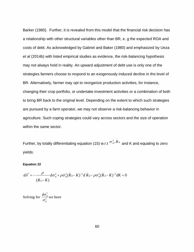
60

Barker (1980). Further, it is revealed from this model that the financial risk decision has

a relationship with other structural variables other than BR, e. g the expected ROA and

costs of debt. As acknowledged by Gabriel and Baker (1980) and emphasized by Ueza

et al (2014b) with listed empirical studies as evidence, the risk-balancing hypothesis

may not always hold in reality. An upward adjustment of debt use is only one of the

strategies farmers choose to respond to an exogenously induced decline in the level of

BR. Alternatively, farmer may opt to reorganize production activities, for instance,

changing their crop portfolio, or undertake investment activities or a combination of both

to bring BR back to the original level. Depending on the extent to which such strategies

are pursued by a farm operator, we may not observe a risk-balancing behavior in

agriculture. Such coping strategies could vary across sectors and the size of operation

within the same sector.

Further, by totally differentiating equation (15) w.r.t 2 , AA R

and K and equating to zero

yields:

Equation 22

* 2 2 2 2 2( ) ( ) 0

( )

A A AA A A

A

d d R K d R R K dK

R K

Solving for 2

2

A

A

d

we have

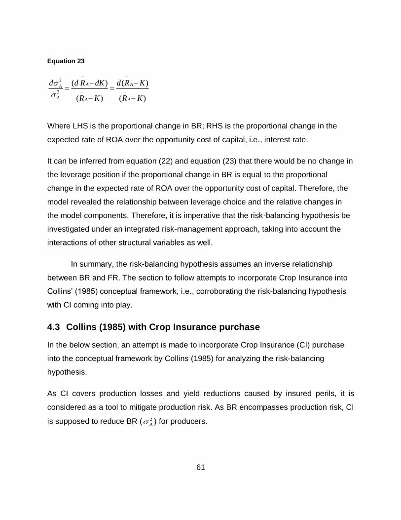
61

Equation 23

2

2

( ) ( )

( ) ( )

A AA

A A A

d d R dK d R K

R K R K

Where LHS is the proportional change in BR; RHS is the proportional change in the

expected rate of ROA over the opportunity cost of capital, i.e., interest rate.

It can be inferred from equation (22) and equation (23) that there would be no change in

the leverage position if the proportional change in BR is equal to the proportional

change in the expected rate of ROA over the opportunity cost of capital. Therefore, the

model revealed the relationship between leverage choice and the relative changes in

the model components. Therefore, it is imperative that the risk-balancing hypothesis be

investigated under an integrated risk-management approach, taking into account the

interactions of other structural variables as well.

In summary, the risk-balancing hypothesis assumes an inverse relationship

between BR and FR. The section to follow attempts to incorporate Crop Insurance into

Collins’ (1985) conceptual framework, i.e., corroborating the risk-balancing hypothesis

with CI coming into play.

4.3 Collins (1985) with Crop Insurance purchase

In the below section, an attempt is made to incorporate Crop Insurance (CI) purchase

into the conceptual framework by Collins (1985) for analyzing the risk-balancing

hypothesis.

As CI covers production losses and yield reductions caused by insured perils, it is

considered as a tool to mitigate production risk. As BR encompasses production risk, CI

is supposed to reduce BR ( 2

A ) for producers.

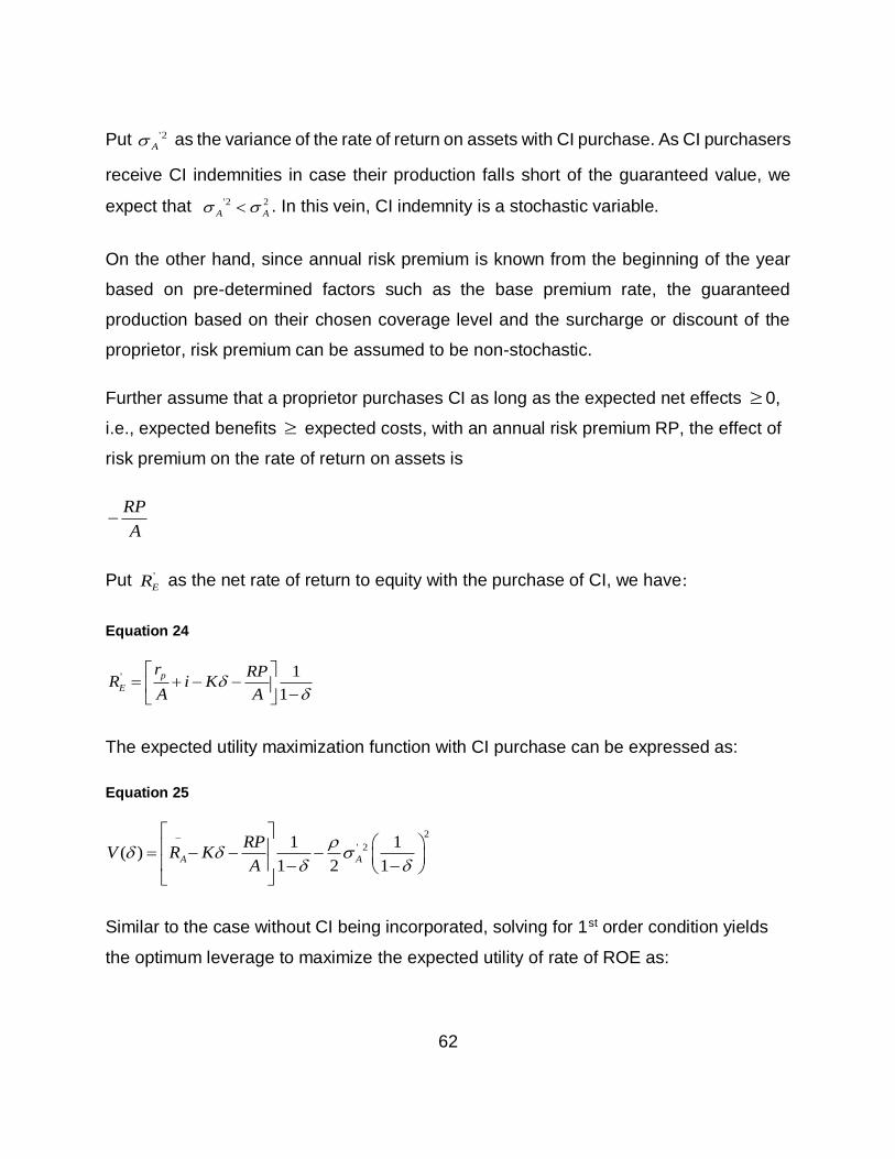
62

Put '2

A as the variance of the rate of return on assets with CI purchase. As CI purchasers

receive CI indemnities in case their production falls short of the guaranteed value, we

expect that '2 2

A A . In this vein, CI indemnity is a stochastic variable.

On the other hand, since annual risk premium is known from the beginning of the year

based on pre-determined factors such as the base premium rate, the guaranteed

production based on their chosen coverage level and the surcharge or discount of the

proprietor, risk premium can be assumed to be non-stochastic.

Further assume that a proprietor purchases CI as long as the expected net effects 0,

i.e., expected benefits expected costs, with an annual risk premium RP, the effect of

risk premium on the rate of return on assets is

RP

A

Put '

ER as the net rate of return to equity with the purchase of CI, we have:

Equation 24

' 1

1

p

E

r RPR i K

A A

The expected utility maximization function with CI purchase can be expressed as:

Equation 25

2

' 21 1( )

1 2 1A A

RPV R K

A

Similar to the case without CI being incorporated, solving for 1st order condition yields

the optimum leverage to maximize the expected utility of rate of ROE as:

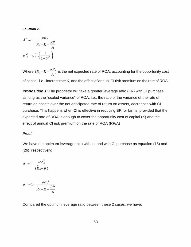
63

Equation 26

' 2*

2

2 ' 2

*

' 1

1' .

1 '

A

A

E A

RPR K

A

Where ( )A

RPR K

A

is the net expected rate of ROA, accounting for the opportunity cost

of capital, i.e., interest rate K, and the effect of annual CI risk premium on the rate of ROA.

Proposition 1: The proprietor will take a greater leverage ratio (FR) with CI purchase

as long as the “scaled variance” of ROA, i.e., the ratio of the variance of the rate of

return on assets over the net anticipated rate of return on assets, decreases with CI

purchase. This happens when CI is effective in reducing BR for farms, provided that the

expected rate of ROA is enough to cover the opportunity cost of capital (K) and the

effect of annual CI risk premium on the rate of ROA (RP/A)

Proof:

We have the optimum leverage ratio without and with CI purchase as equation (15) and

(26), respectively:

2* 1

( )

A

AR K

' 2*' 1 A

A

RPR K

A

Compared the optimum leverage ratio between these 2 cases, we have:

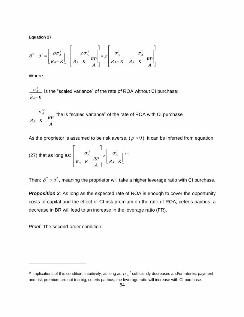
64

Equation 27

2 '2 2 '2'* * A A A A

A AA A

RP RPR K R KR K R K

A A

Where:

2

A

AR K

is the “scaled variance” of the rate of ROA without CI purchase;

'2

A

A

RPR K

A

the is “scaled variance” of the rate of ROA with CI purchase

As the proprietor is assumed to be risk averse, ( 0 ), it can be inferred from equation

(27) that as long as: '2 2

A A

AA

RPR KR K

A

15

Then: '* * , meaning the proprietor will take a higher leverage ratio with CI purchase.

Proposition 2: As long as the expected rate of ROA is enough to cover the opportunity

costs of capital and the effect of CI risk premium on the rate of ROA, ceteris paribus, a

decrease in BR will lead to an increase in the leverage ratio (FR).

Proof: The second-order condition:

15 Implications of this condition: intuitively, as long as '2

A sufficiently decreases and/or interest payment

and risk premium are not too big, ceteris paribus, the leverage ratio will increase with CI purchase.

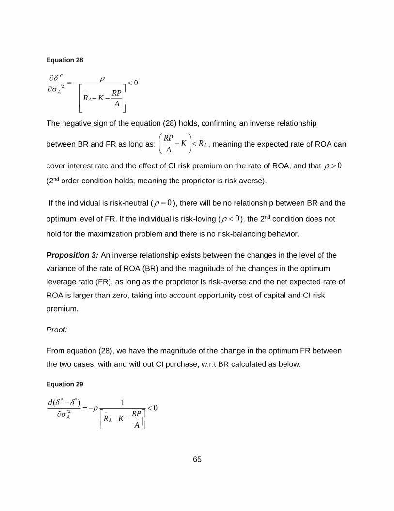
65

Equation 28

*

'2

'0

A

ARP

R KA

The negative sign of the equation (28) holds, confirming an inverse relationship

between BR and FR as long as: A

RPK R

A

, meaning the expected rate of ROA can

cover interest rate and the effect of CI risk premium on the rate of ROA, and that 0

(2nd order condition holds, meaning the proprietor is risk averse).

If the individual is risk-neutral ( 0 ), there will be no relationship between BR and the

optimum level of FR. If the individual is risk-loving ( 0 ), the 2nd condition does not

hold for the maximization problem and there is no risk-balancing behavior.

Proposition 3: An inverse relationship exists between the changes in the level of the

variance of the rate of ROA (BR) and the magnitude of the changes in the optimum

leverage ratio (FR), as long as the proprietor is risk-averse and the net expected rate of

ROA is larger than zero, taking into account opportunity cost of capital and CI risk

premium.

Proof:

From equation (28), we have the magnitude of the change in the optimum FR between

the two cases, with and without CI purchase, w.r.t BR calculated as below:

Equation 29

'* *

'2

( ) 10

AA

d

RPR K

A

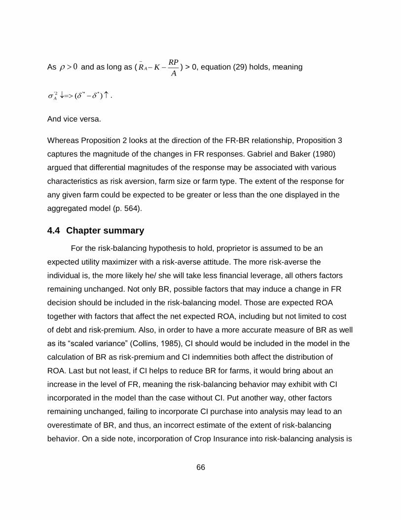
66

As 0 and as long as ( A

RPR K

A

) > 0, equation (29) holds, meaning

'2 '* *( )A .

And vice versa.

Whereas Proposition 2 looks at the direction of the FR-BR relationship, Proposition 3

captures the magnitude of the changes in FR responses. Gabriel and Baker (1980)

argued that differential magnitudes of the response may be associated with various

characteristics as risk aversion, farm size or farm type. The extent of the response for

any given farm could be expected to be greater or less than the one displayed in the

aggregated model (p. 564).

4.4 Chapter summary

For the risk-balancing hypothesis to hold, proprietor is assumed to be an

expected utility maximizer with a risk-averse attitude. The more risk-averse the

individual is, the more likely he/ she will take less financial leverage, all others factors

remaining unchanged. Not only BR, possible factors that may induce a change in FR

decision should be included in the risk-balancing model. Those are expected ROA

together with factors that affect the net expected ROA, including but not limited to cost

of debt and risk-premium. Also, in order to have a more accurate measure of BR as well

as its “scaled variance” (Collins, 1985), CI should would be included in the model in the

calculation of BR as risk-premium and CI indemnities both affect the distribution of

ROA. Last but not least, if CI helps to reduce BR for farms, it would bring about an

increase in the level of FR, meaning the risk-balancing behavior may exhibit with CI

incorporated in the model than the case without CI. Put another way, other factors

remaining unchanged, failing to incorporate CI purchase into analysis may lead to an

overestimate of BR, and thus, an incorrect estimate of the extent of risk-balancing

behavior. On a side note, incorporation of Crop Insurance into risk-balancing analysis is

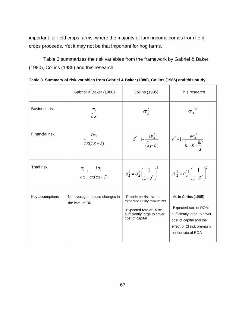
67

important for field crops farms, where the majority of farm income comes from field

crops proceeds. Yet it may not be that important for hog farms.

Table 3 summarizes the risk variables from the framework by Gabriel & Baker

(1980), Collins (1985) and this research.

Table 3. Summary of risk variables from Gabriel & Baker (1980), Collins (1985) and this study

Gabriel & Baker (1980) Collins (1985) This research

Business risk

Financial risk

Total risk

Key assumptions No leverage-induced changes in

the level of BR.

-Proprietor: risk-averse expected utility maximizer

-Expected rate of ROA: sufficiently large to cover cost of capital

-As in Collins (1985)

-Expected rate of ROA:

sufficiently large to cover

cost of capital and the

effect of CI risk premium

on the rate of ROA

68

5 Chapter 5: DATA, VARIABLE MEASURES AND DESCRIPTIVE STATISTICS


The purpose of this chapter is to describe the data and define the variables used

to investigate the risk-balancing behavior in Ontario hog sector. The chapter is

composed of two broad sections. The first section describes data features and variable

definition. The second section provides descriptive statistics of the key variables and

explain alternative risk measurements to be employed in the empirical analysis.16

5.2 Data and variable definition

5.2.1 Data sources and features

The data used in this study comes from Ontario Farm Income Database (OFID), which

is a longitudinal data set compiled from the tax file records of participating farms in

Ontario. Data on AgriStability payments under CAIS/ BRM programs are also included in

this data set. Additionally, we used aggregate data on changes in Ontario farm land value

from Farm Credit Canada17.

The original data set consisted of 22,462 observations covering 4,353 farms from

2003 to 2014. From the original dataset, 10,149 observations were excluded from the

sample because they have negative interest expenses and are presumed to have

measurement errors. Since business risk can influence financial risk only with a lag, farms

to be included in this study need to be present in at least two consecutive years during

the study period. As a result, 285 observations that did not satisfy this condition were also

dropped. As debts show up in the denominator of the Cost of debt variable (interest/debt),

553 observations that have debt value equal to “0” or NAs were excluded from the

16 Crop Insurance is not incorporated into our empirical analysis due to the unavailability of Crop Insurance data at farm-level.

17 Data was obtained from Farmland values report – Historical values (Farm Credit Canada, 2017)

69

sample18. After removing all these observations, we have a panel dataset of 11,462

observations consisting of 2,036 farms for the 2003-2014 period.

5.2.2 Variable definition and empirical measurement

Risk measures

Following the empirical literature in measuring business risk based on Net

Operating Income (NOI) or Return on Asset, we used NOI to construct our risk measures

due to the lack of balance sheet.19

Business risk (BR)

The most commonly used measurement of BR in the literature is the coefficient of

variation (CV) of either NOI or CV of return of assets. Corresponding to this way of

measuring BR, we computed CV of NOI as our initial measure of BR. In particular, 2-year

rolling standard deviation over 2-year moving average of NOI was computed to construct

this BR-CV measurement20. Notably, the use of CV of NOI as a measure of risk implies

that NOI is normally distributed. Also, this measurement cannot tell whether the variable

has a tendency for more values to fall in the upper, i.e., the right, or lower, i.e., the left,

tail of the distribution.

18 Additionally, farms that have revenue equal to $1 are presumed to be input errors and were removed

from the sample.

19 Besides, we employed Revenue and Arm’s length salary to compute NOI since the majority of Total Operating Revenue showed up with negative values and Cost of Goods Sold for a large number of observations amounted to millions of dollars, which were presumed to be measurement errors.

20 Our rationale in choosing the 2-year window is the 4-year time span of CAIS as well as BRM. While a number previous studies choose a longer time-window for the CV measurement, in our case, a longer time-span would lead to overlap AgriStability payments across different policy regimes. In addition, fewer observations would be retained in the sample if we used a longer window in computing the CV measure. Neither was considered desirable for this study.

70

Subsequently, we tested if the NOI variable is normally distributed for each farm

size category. An attempt was then made to measure BR as rolling skewness21 of NOI

when the null hypothesis of normal distribution was rejected. By using skewness, we

focus on the tails of the distribution, i.e., the infrequent and extreme losses or gains rather

than on variations around the mean, which stands for small and frequent gains or losses

from risk perspective. Skewness tells us if the distribution of NOI is skewed or not, and if

it is skewed to the left, i.e., more downside risks or to the right, i.e., more upside risks.

Financial risk (FR)

FR is measured in two ways. First, we followed the empirical model by Gabriel and

Barker (1980) in constructing FR measure as the ratio of interest expense to the NOI

variable. This is hereinafter referred to as FR-magnitude measurement. Although

longitudinal data allows for heterogeneity across individuals and overtime, we tried an

alternative way of measuring FR as the CV of Interest expense to NOI ratio on the ground

that variations imply uncertainty and risk. In particular, FR-CV measurement was

computed as the 2-year rolling standard deviation over the 2-year moving average of the

Interest expenses-NOI ratio.

Explanatory variables

Business risk in the previous year, measured in two ways, i.e., 1-year lagged CV and 1-

year lagged rolling skewness of NOI. In each way of measurement, AgriStability

payments under CAIS/ BRM were incorporated into the computation of risk to compare

the risk level with and without program payments.

Farm diversification, measured by Herfindahl index22 at farm level and ranges from 0

to 1. This index represents revenue allocation among various operations (e.g., beef,

21 Skewness requires a rolling window of at least 3-years for the statistic to be computable.

22 Herfindahl index: 2

1

( )n

i

i

H share

71

hog, dairy, grain etc.). A lower index value indicates a greater level of diversification for

farms and farm diversification could be considered as a risk management strategy. We

expect an increase in the level of diversification, i.e., the lower in the index, to be

associated with an increase in the leverage taken. Besides, farms with different

diversification levels may have different risk-balancing behaviors.

Cost of debt in the previous year, measured by interest expense to debt ratio. We

would expect farms with a high historical cost of debt to be less likely to take on more

leverage in the current period.

Change in farm land value in previous year, being Ontario farmland appreciation

rates. This variable is included to account for changes in farm land value between

years, since relevant information at farm level is not available. As farms may use land

as collateral for their loan, changes in the prices of farmland are assumed to affect farm

liquidity as credit adjusts to new equity values (Collins, 1985). In this sense, farm land

value can be used as proxy for farm asset. However, as hog farming in Ontario is not

land intensive, change in farmland value may or may not have a significant effect on

farm FR.

Table 4 provides a summary of variables and expected signs in our model

estimation.

Table 4. Variable summary

Variables Definition/ Ways of measurement Measurement

unit

Expected

signs

Response variable

Financial risk i. Interest expenses/ NOI

ii. CV of Interest expenses/ NOI

Unit-free

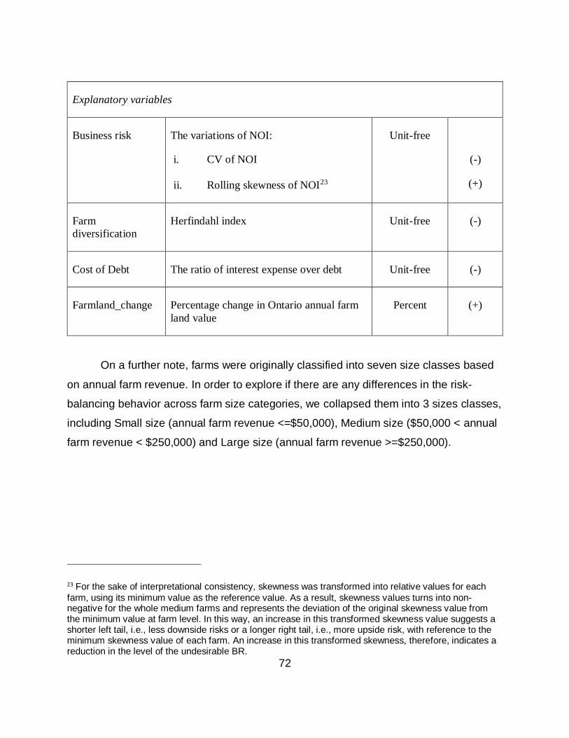
72

Explanatory variables

Business risk The variations of NOI:

i. CV of NOI

ii. Rolling skewness of NOI23

Unit-free

(-)

(+)

Farm

diversification

Herfindahl index Unit-free (-)

Cost of Debt The ratio of interest expense over debt Unit-free (-)

Farmland_change Percentage change in Ontario annual farm

land value

Percent (+)

On a further note, farms were originally classified into seven size classes based

on annual farm revenue. In order to explore if there are any differences in the risk-

balancing behavior across farm size categories, we collapsed them into 3 sizes classes,

including Small size (annual farm revenue <=$50,000), Medium size ($50,000 < annual

farm revenue < $250,000) and Large size (annual farm revenue >=$250,000).

23 For the sake of interpretational consistency, skewness was transformed into relative values for each

farm, using its minimum value as the reference value. As a result, skewness values turns into non-negative for the whole medium farms and represents the deviation of the original skewness value from the minimum value at farm level. In this way, an increase in this transformed skewness value suggests a shorter left tail, i.e., less downside risks or a longer right tail, i.e., more upside risk, with reference to the minimum skewness value of each farm. An increase in this transformed skewness, therefore, indicates a reduction in the level of the undesirable BR.

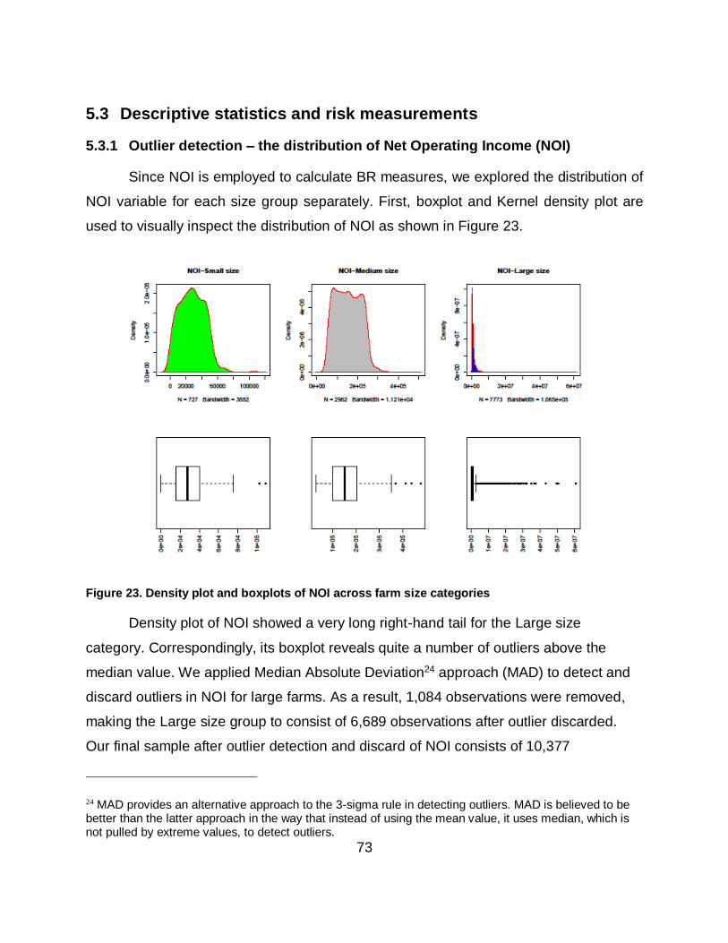
73

5.3 Descriptive statistics and risk measurements

5.3.1 Outlier detection – the distribution of Net Operating Income (NOI)

Since NOI is employed to calculate BR measures, we explored the distribution of

NOI variable for each size group separately. First, boxplot and Kernel density plot are

used to visually inspect the distribution of NOI as shown in Figure 23.

Figure 23. Density plot and boxplots of NOI across farm size categories

Density plot of NOI showed a very long right-hand tail for the Large size

category. Correspondingly, its boxplot reveals quite a number of outliers above the

median value. We applied Median Absolute Deviation24 approach (MAD) to detect and

discard outliers in NOI for large farms. As a result, 1,084 observations were removed,

making the Large size group to consist of 6,689 observations after outlier discarded.

Our final sample after outlier detection and discard of NOI consists of 10,377

24 MAD provides an alternative approach to the 3-sigma rule in detecting outliers. MAD is believed to be better than the latter approach in the way that instead of using the mean value, it uses median, which is not pulled by extreme values, to detect outliers.

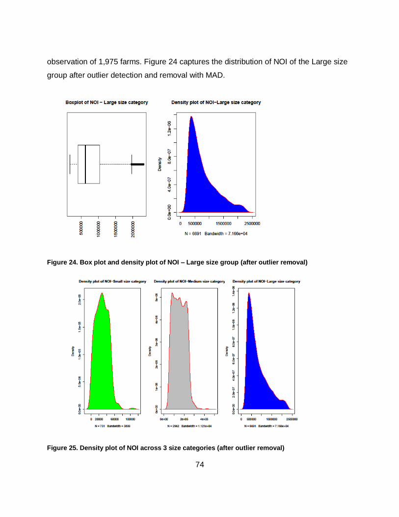
74

observation of 1,975 farms. Figure 24 captures the distribution of NOI of the Large size

group after outlier detection and removal with MAD.

Figure 24. Box plot and density plot of NOI – Large size group (after outlier removal)

Figure 25. Density plot of NOI across 3 size categories (after outlier removal)

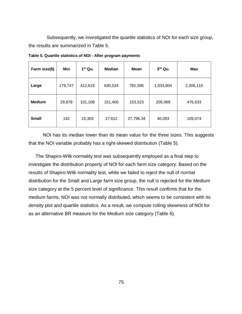
75

Subsequently, we investigated the quartile statistics of NOI for each size group,

the results are summarized in Table 5.

Table 5. Quartile statistics of NOI - After program payments

NOI has its median lower than its mean value for the three sizes. This suggests

that the NOI variable probably has a right-skewed distribution (Table 5).

The Shapiro-Wilk normality test was subsequently employed as a final step to

investigate the distribution property of NOI for each farm size category. Based on the

results of Shapiro-Wilk normality test, while we failed to reject the null of normal

distribution for the Small and Large farm size group, the null is rejected for the Medium

size category at the 5 percent level of significance. This result confirms that for the

medium farms, NOI was not normally distributed, which seems to be consistent with its

density plot and quartile statistics. As a result, we compute rolling skewness of NOI for

as an alternative BR measure for the Medium size category (Table 6).

Farm size($) Min 1st Qu. Median Mean 3rd Qu. Max

Large 179,747 412,619 630,524 781,595 1,033,804 2,306,115

Medium 29,878 101,108 151,400 153,523 205,068 476,633

Small 142 15,303 27,612 27,796.34 40,093 109,074

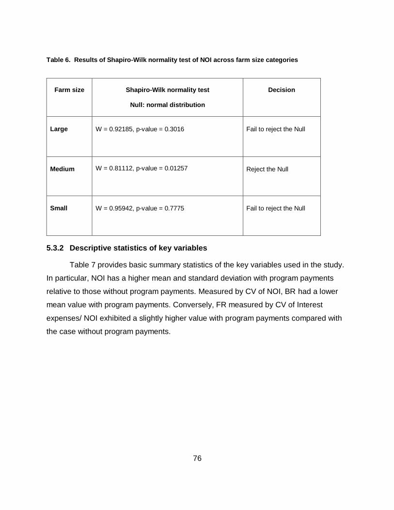
76

Table 6. Results of Shapiro-Wilk normality test of NOI across farm size categories

5.3.2 Descriptive statistics of key variables

Table 7 provides basic summary statistics of the key variables used in the study.

In particular, NOI has a higher mean and standard deviation with program payments

relative to those without program payments. Measured by CV of NOI, BR had a lower

mean value with program payments. Conversely, FR measured by CV of Interest

expenses/ NOI exhibited a slightly higher value with program payments compared with

the case without program payments.

Farm size

Shapiro-Wilk normality test

Null: normal distribution

Decision

Large W = 0.92185, p-value = 0.3016

Fail to reject the Null

Medium W = 0.81112, p-value = 0.01257

Reject the Null

Small W = 0.95942, p-value = 0.7775

Fail to reject the Null

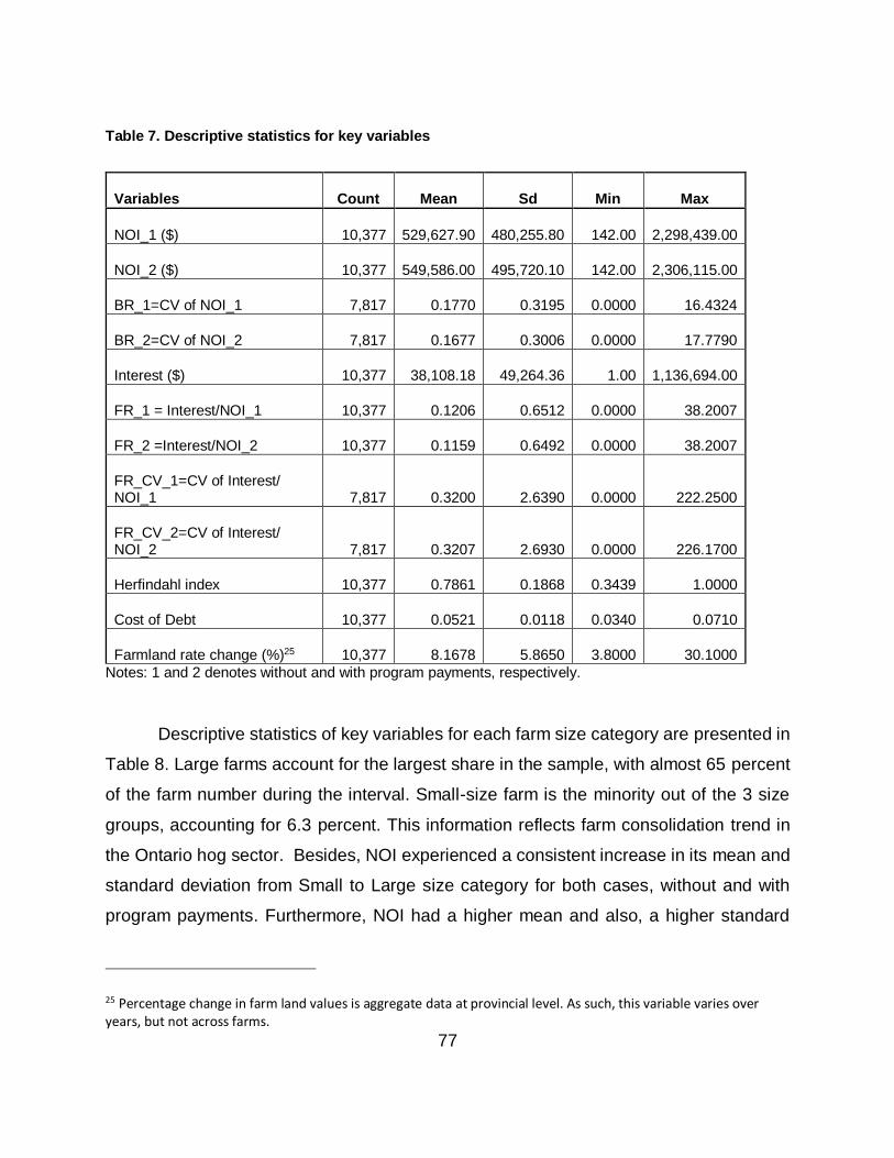
77

Table 7. Descriptive statistics for key variables

Notes: 1 and 2 denotes without and with program payments, respectively.

Descriptive statistics of key variables for each farm size category are presented in

Table 8. Large farms account for the largest share in the sample, with almost 65 percent

of the farm number during the interval. Small-size farm is the minority out of the 3 size

groups, accounting for 6.3 percent. This information reflects farm consolidation trend in

the Ontario hog sector. Besides, NOI experienced a consistent increase in its mean and

standard deviation from Small to Large size category for both cases, without and with

program payments. Furthermore, NOI had a higher mean and also, a higher standard

25 Percentage change in farm land values is aggregate data at provincial level. As such, this variable varies over years, but not across farms.

Variables Count Mean Sd Min Max

NOI_1 ($) 10,377 529,627.90 480,255.80 142.00 2,298,439.00

NOI_2 ($) 10,377 549,586.00 495,720.10 142.00 2,306,115.00

BR_1=CV of NOI_1 7,817 0.1770 0.3195 0.0000 16.4324

BR_2=CV of NOI_2 7,817 0.1677 0.3006 0.0000 17.7790

Interest ($) 10,377 38,108.18 49,264.36 1.00 1,136,694.00

FR_1 = Interest/NOI_1 10,377 0.1206 0.6512 0.0000 38.2007

FR_2 =Interest/NOI_2 10,377 0.1159 0.6492 0.0000 38.2007

FR_CV_1=CV of Interest/ NOI_1 7,817 0.3200 2.6390 0.0000 222.2500

FR_CV_2=CV of Interest/ NOI_2 7,817 0.3207 2.6930 0.0000 226.1700

Herfindahl index 10,377 0.7861 0.1868 0.3439 1.0000

Cost of Debt 10,377 0.0521 0.0118 0.0340 0.0710

Farmland rate change (%)25 10,377 8.1678 5.8650 3.8000 30.1000

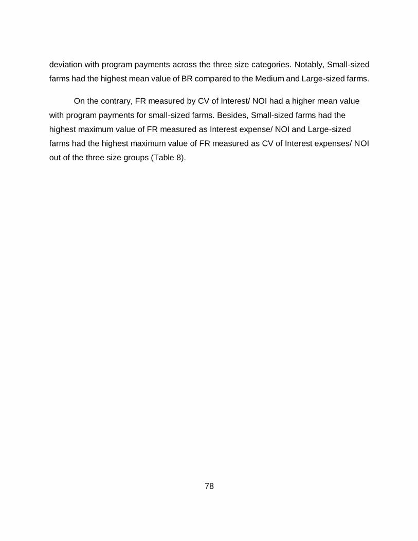
78

deviation with program payments across the three size categories. Notably, Small-sized

farms had the highest mean value of BR compared to the Medium and Large-sized farms.

On the contrary, FR measured by CV of Interest/ NOI had a higher mean value

with program payments for small-sized farms. Besides, Small-sized farms had the

highest maximum value of FR measured as Interest expense/ NOI and Large-sized

farms had the highest maximum value of FR measured as CV of Interest expenses/ NOI

out of the three size groups (Table 8).

79

Table 8. Descriptive Statistics by farm size categories

Small Medium Large

mean sd min max mean sd min max mean sd min max

NOI_1 ($) 26,042.750 14,147.590 142.000 49,979.000 146,843.000 57,163.070 29,878.000 249,982.000 753,797.000 462,243.300 174,844.000 2,298,439.000

NOI_2 ($) 27,948.330 16,111.670 142.000 109,074.000 153,523.100 61,595.610 29,878.000 476,633.000 781,594.500 476,107.200 179,746.600 2,306,115.000

BR_1=CV of NOI_1

0.472 1.098 0.000 16.432 0.198 0.258 0.000 3.919 0.145 0.134 0.000 1.038

BR_2=CV of NOI_2

0.465 1.009 0.000 17.180 0.190 0.253 0.000 3.983 0.102 0.130 0.000 1.053

Interest expense ($)

6,818.730 9,751.590 3.000 101,574.000 14,529.500 16,653.430 2.000 166,162.000 51,945.800 55,571.060 1.000 1,136,694.000

FR_1 = Interest/NOI_1

0.597 2.386 0.000 38.201 0.107 0.140 0.000 2.732 0.075 0.070 0.000 1.466

FR_2 =Interest/NOI_2

0.581 2.383 0.000 38.201 0.102 0.132 0.000 2.732 0.071 0.064 0.000 1.466

FR_CV_1=CV of Interest/ NOI_1

0.437 0.364 0.000 1.409 0.353 1.443 0.000 64.403 0.304 0.071 0.000 222.252

FR_CV_2=CV of Interest/ NOI_2

0.447 0.362 0.003 1.409 0.352 1.519 0.000 67.953 0.298 3.124 0.000 226.166

Herfindahl index 0.726 0.224 0.343 1.000 0.718 0.191 0.360 1.000 0.823 0.169 0.349 1.000

Cost of Debt = Interest/ Debt

0.053 0.012 0.034 0.071 0.054 0.011 0.034 0.071 0.051 0.012 0.034 0.071

N 726 2,962 6,689

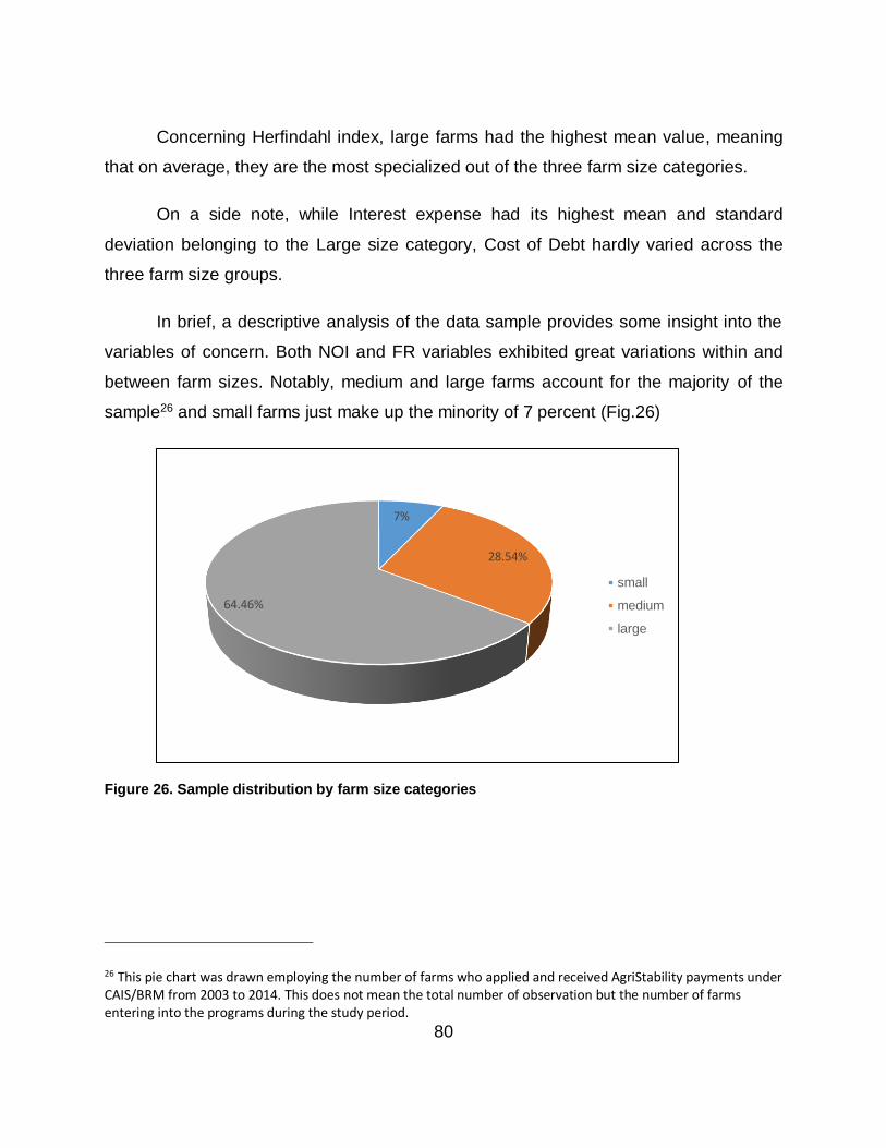
80

Concerning Herfindahl index, large farms had the highest mean value, meaning

that on average, they are the most specialized out of the three farm size categories.

On a side note, while Interest expense had its highest mean and standard

deviation belonging to the Large size category, Cost of Debt hardly varied across the

three farm size groups.

In brief, a descriptive analysis of the data sample provides some insight into the

variables of concern. Both NOI and FR variables exhibited great variations within and

between farm sizes. Notably, medium and large farms account for the majority of the

sample26 and small farms just make up the minority of 7 percent (Fig.26)

Figure 26. Sample distribution by farm size categories

26 This pie chart was drawn employing the number of farms who applied and received AgriStability payments under CAIS/BRM from 2003 to 2014. This does not mean the total number of observation but the number of farms entering into the programs during the study period.

7%

28.54%

64.46%

small

medium

large

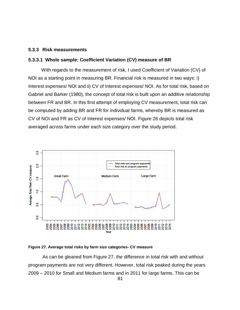
81

5.3.3 Risk measurements

5.3.3.1 Whole sample: Coefficient Variation (CV) measure of BR

With regards to the measurement of risk, I used Coefficient of Variation (CV) of

NOI as a starting point in measuring BR. Financial risk is measured in two ways: i)

Interest expenses/ NOI and ii) CV of Interest expenses/ NOI. As for total risk, based on

Gabriel and Barker (1980), the concept of total risk is built upon an additive relationship

between FR and BR. In this first attempt of employing CV measurement, total risk can

be computed by adding BR and FR for individual farms, whereby BR is measured as

CV of NOI and FR as CV of Interest expenses/ NOI. Figure 26 depicts total risk

averaged across farms under each size category over the study period.

Figure 27. Average total risks by farm size categories- CV measure

As can be gleaned from Figure 27, the difference in total risk with and without

program payments are not very different. However, total risk peaked during the years

2009 – 2010 for Small and Medium farms and in 2011 for large farms. This can be

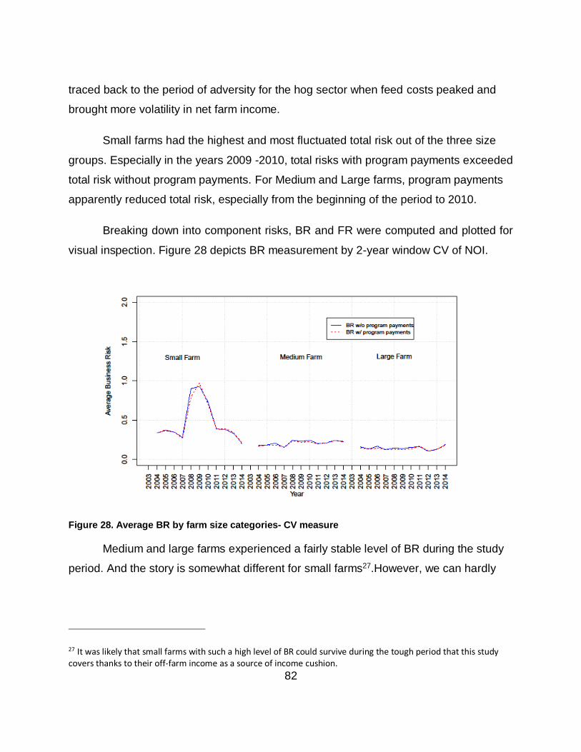
82

traced back to the period of adversity for the hog sector when feed costs peaked and

brought more volatility in net farm income.

Small farms had the highest and most fluctuated total risk out of the three size

groups. Especially in the years 2009 -2010, total risks with program payments exceeded

total risk without program payments. For Medium and Large farms, program payments

apparently reduced total risk, especially from the beginning of the period to 2010.

Breaking down into component risks, BR and FR were computed and plotted for

visual inspection. Figure 28 depicts BR measurement by 2-year window CV of NOI.

Figure 28. Average BR by farm size categories- CV measure

Medium and large farms experienced a fairly stable level of BR during the study

period. And the story is somewhat different for small farms27.However, we can hardly

27 It was likely that small farms with such a high level of BR could survive during the tough period that this study covers thanks to their off-farm income as a source of income cushion.

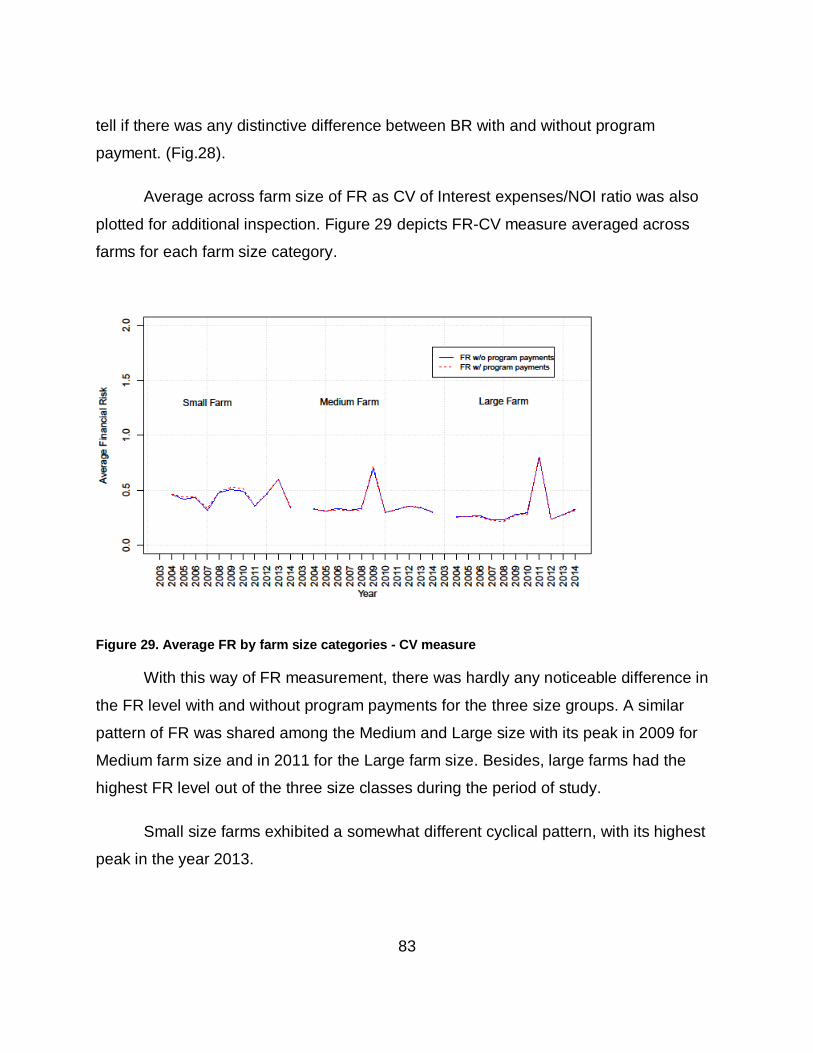
83

tell if there was any distinctive difference between BR with and without program

payment. (Fig.28).

Average across farm size of FR as CV of Interest expenses/NOI ratio was also

plotted for additional inspection. Figure 29 depicts FR-CV measure averaged across

farms for each farm size category.

Figure 29. Average FR by farm size categories - CV measure

With this way of FR measurement, there was hardly any noticeable difference in

the FR level with and without program payments for the three size groups. A similar

pattern of FR was shared among the Medium and Large size with its peak in 2009 for

Medium farm size and in 2011 for the Large farm size. Besides, large farms had the

highest FR level out of the three size classes during the period of study.

Small size farms exhibited a somewhat different cyclical pattern, with its highest

peak in the year 2013.

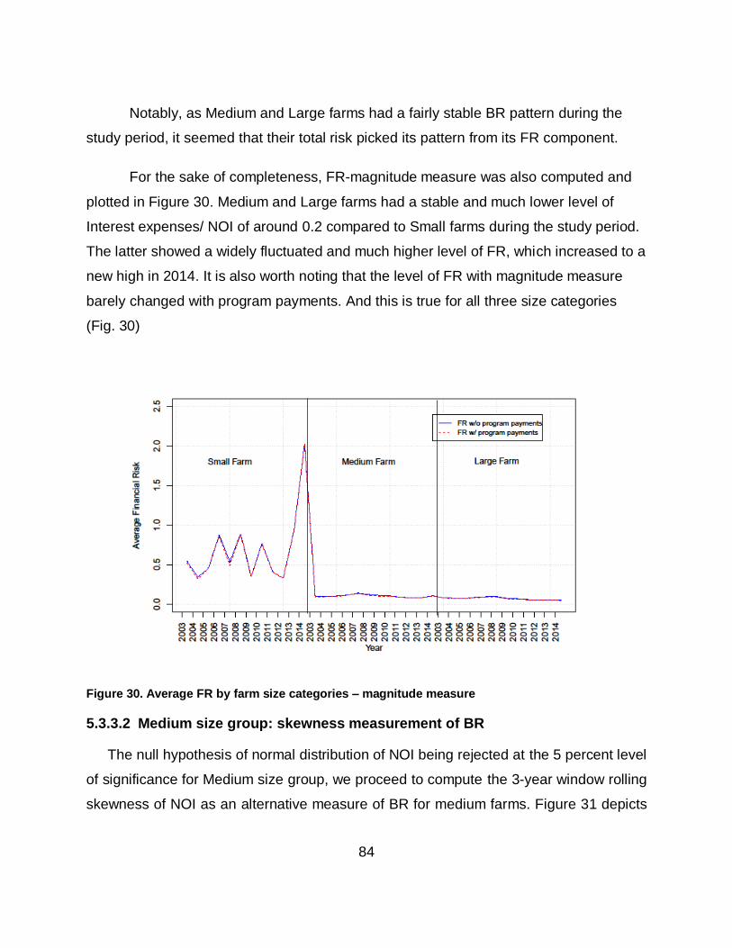
84

Notably, as Medium and Large farms had a fairly stable BR pattern during the

study period, it seemed that their total risk picked its pattern from its FR component.

For the sake of completeness, FR-magnitude measure was also computed and

plotted in Figure 30. Medium and Large farms had a stable and much lower level of

Interest expenses/ NOI of around 0.2 compared to Small farms during the study period.

The latter showed a widely fluctuated and much higher level of FR, which increased to a

new high in 2014. It is also worth noting that the level of FR with magnitude measure

barely changed with program payments. And this is true for all three size categories

(Fig. 30)

Figure 30. Average FR by farm size categories – magnitude measure

5.3.3.2 Medium size group: skewness measurement of BR

The null hypothesis of normal distribution of NOI being rejected at the 5 percent level

of significance for Medium size group, we proceed to compute the 3-year window rolling

skewness of NOI as an alternative measure of BR for medium farms. Figure 31 depicts

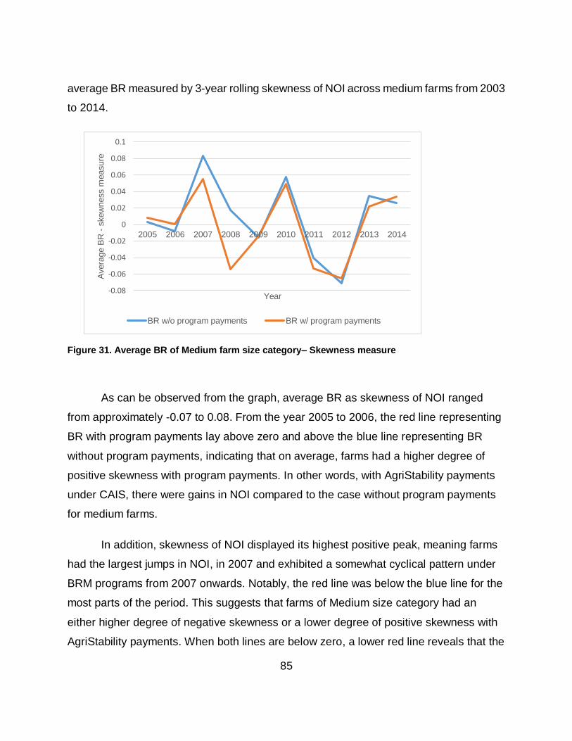
85

average BR measured by 3-year rolling skewness of NOI across medium farms from 2003

to 2014.

Figure 31. Average BR of Medium farm size category– Skewness measure

As can be observed from the graph, average BR as skewness of NOI ranged

from approximately -0.07 to 0.08. From the year 2005 to 2006, the red line representing

BR with program payments lay above zero and above the blue line representing BR

without program payments, indicating that on average, farms had a higher degree of

positive skewness with program payments. In other words, with AgriStability payments

under CAIS, there were gains in NOI compared to the case without program payments

for medium farms.

In addition, skewness of NOI displayed its highest positive peak, meaning farms

had the largest jumps in NOI, in 2007 and exhibited a somewhat cyclical pattern under

BRM programs from 2007 onwards. Notably, the red line was below the blue line for the

most parts of the period. This suggests that farms of Medium size category had an

either higher degree of negative skewness or a lower degree of positive skewness with

AgriStability payments. When both lines are below zero, a lower red line reveals that the

-0.08

-0.06

-0.04

-0.02

0

0.02

0.04

0.06

0.08

0.1

2005 2006 2007 2008 2009 2010 2011 2012 2013 2014

Avera

ge B

R -

skew

ness m

easure

Year

BR w/o program payments BR w/ program payments

86

distribution of NOI had a longer left tail, meaning a higher level of downside risk, or

farms incurred larger drops in NOI with program payments. When both lines are above

zero, a lower red line denotes a distribution with a shorter right tail, i.e., a lower lever of

upside risk.

5.4 Chapter summary

In this chapter, we provided a descriptive statistics of the sample data for the three

farm size categories and defined alternative ways of risk measurements for empirical

analysis. BR was measured by CV and skewness of NOI, and FR was measured by

Interest expense/ NOI and the CV of this ratio.

Our graphical examination of the risk-measurements for Ontario hog sector

suggested that total risk with CV measurement peaked during the years 2009 – 2010 for

small and medium farms and in 2011 for large farms. This can be traced back to the

period of adversity for the sector when feed costs rocketed and brought more volatility in

net farm income. In addition, with BR measured as CV of NOI, small farms had the

highest level and most fluctuated pattern of BR out of the three farm size categories.

With BR measured as skewness of NOI, it was revealed that medium farms

experienced larger gains in NOI with AgriStability payments under CAIS. Under BRM

programs from 2007 onwards, farms exhibited either a higher degree of negative

skewness, i.e., farms incurred larger drops in NOI, or a lower degree of positive

skewness, i.e., farms incurred a lower level of upside risk, with AgriStability payments.

In a nutshell, our graphical examination of the risk measurements suggests that

apparently, there was hardly a conspicuous difference in the risk levels with and without

program payments for the three farm size categories during the study period. A formal

test would therefore be conducted in Chapter 6 to confirm the risk-reducing effects of

CAIS/ AgriStability payments on the hog sector in Ontario.

87

6 CHAPTER 6: RESEARCH METHODS AND EMPIRICAL RESULTS


The first section of this chapter discusses empirical approaches employed to

investigate the effectiveness of CAIS/ BRM programs and the risk-balancing behavior in

Ontario hog sector for the 2003-2014 period. Two approaches were applied to

investigate the risk-balancing hypothesis: the correlation coefficient analysis and the

regression analysis. Under the latter approach, model specification and estimation

method are further presented. The second sections analyses empirical results based on

the discussed approaches.

6.2 Empirical approaches

6.2.1 Effectiveness of CAIS/AgriStability payments

One-tailed paired t-test28 was employed to test for the effectiveness of CAIS/

BRM in reducing BR for farms under different size categories. The null hypothesis is no

difference in mean BR without and mean BR with program payments. Alternative

hypothesis is the difference (mean BR_wo – mean BR_with) is significantly greater than

zero. While p-value tells us the significance of the effect, the magnitude of the sample

estimate reveal the strength of the effect.

6.2.2 Extent of risk-balancing

6.2.2.1 Correlation coefficient analysis

The first approach employed to investigate the extent of risk-balancing is to

analyze the correlation coefficient between the 1-year lagged BR and current year FR.

28 : 0dHo ;

2

( ) /

[ ( )]

( 1)( )

i

i

i

D Nt

DD

NN N

88

In particular, a negative correlation coefficient suggests that the current year FR level

moves in an opposite direction with the previous year’s level of BR, thus providing

evidence of risk-balancing. Remarkably, this correlation coefficient approach fails to

account for factors other than BR that could potentially influence the FR decision. This

limitation could be overcome by the regression approach to be presented in the next

section.

6.2.2.2 Regression analysis

Our main approach to investigate risk-balancing in this study is to regress current

period FR measure against the historical BR level and other relevant factors.

6.2.2.2.1 Model specification

Given the temporal aspect of the risk-balancing hypothesis, most of explanatory

variables in our regression model are employed in lagged form. The econometric model

is specified in equation 30:

Equation 30

, 1 , 1 2 , 3 , 1 4 1 ,Cos _i t i i t i t i t t i tFR BR Herfindahl tofDebt Farmland change

Where

,i tFR is current period FR measure; , 1i tBR

is the 1-year lagged BR measure; ,i tHerfindahl

is farm diversification measured by Herfindahl index; , 1Cos i ttofDebt

is the 1-year lagged

ratio of interest expenses over outstanding debt; 1_ tFarmland change is the 1-year

lagged of annual percentage change in Ontario farmland value of the 1tyear .

On a further note, as great heterogeneity of key variables across farm size

categories was showed in our panel descriptive statistics in the previous chapter,we run

separate regressions to investigate the risk-balancing behavior for each farm size class,

i.e., the Small, Medium and Large size group.

89

6.2.2.2.2 Estimation method

First, pooled OLS was used as a natural starting point to examine the models. If

individual effect (cross-sectional or time specific effect) does not exist, OLS produces

efficient and consistent parameter estimates.

Subsequently, panel data models of either Fixed Effect Model (FEM) or Random

Effect Model (REM) was employed. Fixed-effects are tested by F-test, and random

effects are examined by the Lagrange Multiplier (LM) test (Breusch and Pagan, 1980).

Based on Greene (2000), the FEM is generally expressed as:

Equation 31

1 2 3 ...it i it it ity x z u

The FEM allows each cross-section unit to have its own intercept value, which is denoted

by 1i . While it is allowed to vary across entities, 1i is time-invariant.

In the random-effects model, the intercept 1i is assumed to be a random variable with

mean value of 1 and could be expressed as

1 1i i

Being a random error term with mean equal to zero and variance 2 , i captures

the individual differences in the intercept value of each entity. Therefore, i is also

referred to as the cross-section or individual specific error component. Under these

circumstances, the model could be re-written as:

Equation 32

1 2 3 ...it it it ity x z

Where it it itu

90

It is worth noticing that the REM is based on the assumption of no correlation

between the error term and explanatory variables in the model. Which model FEM or

REM is more appropriate depends on our assumption about the likely correlation

between the cross-section specific error component and the explanatory variables

based on our understanding of the data set in use. If they are uncorrelated, REM is

more efficient as it reduces the number of parameters to be estimated. Otherwise REM

will produce inconsistent estimates.

Taking into account the assumption under REM, this estimation method appears

to be more suitable for experimental environment, where variables have random values.

Also, FEM seems to be more appropriate to be employed to estimate the variables in our

dataset, as all the explanatory variables are time-variant. This reasoning is to be validated

by Hausman test, which is used to decide if FEM or REM is more appropriate. The test

statistics has an asymptotic chi-square distribution. If the computed chi-square value

exceeds the critical chi-square value, the null hypothesis that the two estimates should

not differ systematically is rejected and FEM is preferred to REM.

Based on the results of our hypothesis testing of serial correlation, cross-

sectional dependence and heteroscedasticity, we computed the heteroscedasticity and/

or autocorrelation consistent covariance estimator in order to obtain the appropriate

standard errors and test statistics of the corresponding model estimation.

After estimating the model with the selected estimation method and robust

standard errors, I conducted model validation by performing F- test (robust) for model

overall significance and checking for multicollinearity using VIF and correlation matrix

with details to follow.

6.2.2.2.3 Model validation

We validate the econometric model by testing the model overall significance and check

for its multicollinearity.

91

To test the overall significance of a multiple regression, the F-test is used to test the

hypothesis:

0 2 3: ... 0kH

Given the k-variable regression model

With F-statistics: / / ( 1)

/ / ( )

ESS df ESS kF

RSS df RSS n k

If the p-value of F computed from the above equation is sufficiently low, 0H can be

rejected.

As a final step of model validation, we check for multicollinearity to see if there

exists a perfect or exact relationship among the explanatory variables by computing

correlation matrix and Variance Inflation Factor (VIF).

Examination of correlation matrix: large correlation coefficients in the correlation

matrix of explanatory variables indicate multicollinearity. If there is perfect multicollinearity

between any two explanatory variables, the correlation coefficient between these two

variables will approach unity.

Examination of VIF: the VIF quantifies the extent of multicollinearity in an OLS

regression analysis, which is calculated as:

2

1

1j

j

VIFR

Where 2

jR denotes the coefficient of determination when jx is regressed on all other

explanatory variables in the model.

VIF ranges from 1 . 1VIF when 2 0jR , i.e., the thj variable is not linearly related

to the other explanatory variables in the model. VIF when 2 1jR , i.e., the thj variable

is linearly related to the other explanatory variables in the model.

As multicollinearity is not sensitive to estimation methods, we conduct this check

for the respective pooled OLS models.

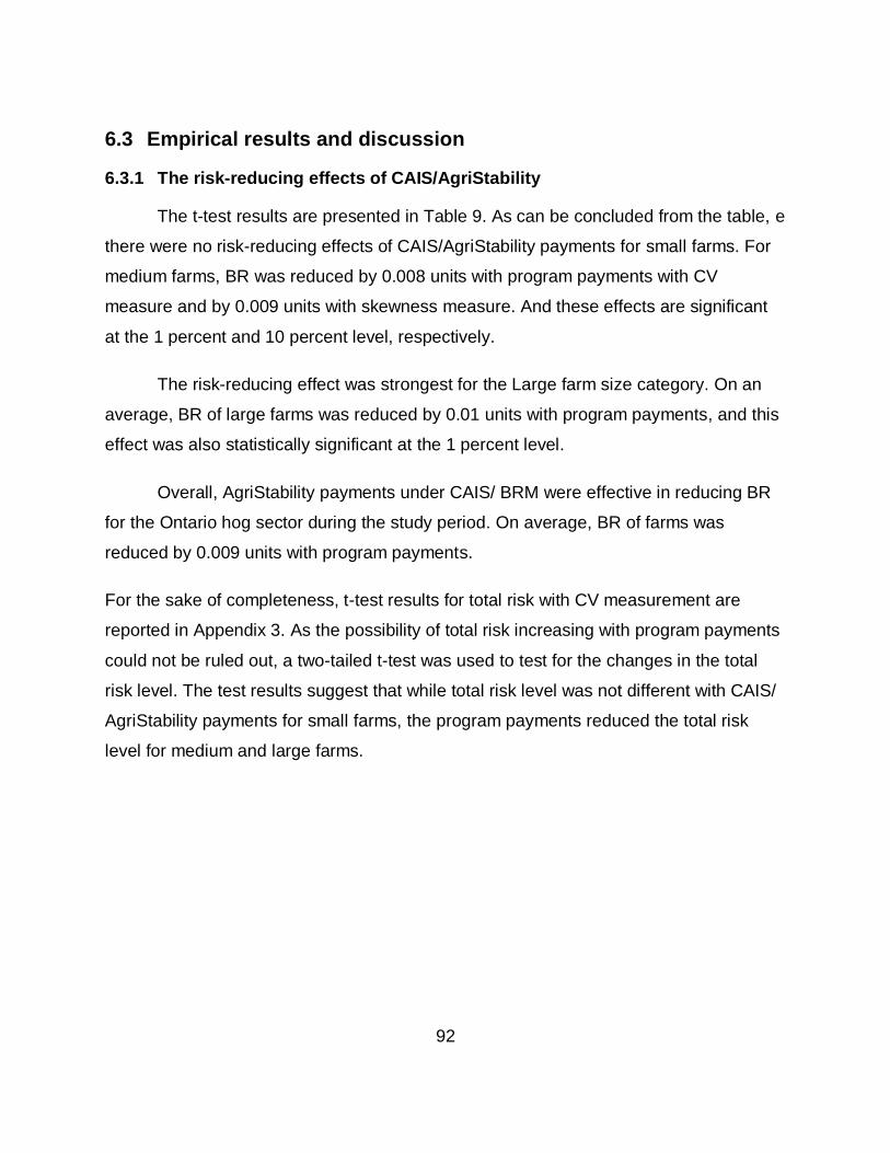
92

6.3 Empirical results and discussion

6.3.1 The risk-reducing effects of CAIS/AgriStability

The t-test results are presented in Table 9. As can be concluded from the table, e

there were no risk-reducing effects of CAIS/AgriStability payments for small farms. For

medium farms, BR was reduced by 0.008 units with program payments with CV

measure and by 0.009 units with skewness measure. And these effects are significant

at the 1 percent and 10 percent level, respectively.

The risk-reducing effect was strongest for the Large farm size category. On an

average, BR of large farms was reduced by 0.01 units with program payments, and this

effect was also statistically significant at the 1 percent level.

Overall, AgriStability payments under CAIS/ BRM were effective in reducing BR

for the Ontario hog sector during the study period. On average, BR of farms was

reduced by 0.009 units with program payments.

For the sake of completeness, t-test results for total risk with CV measurement are

reported in Appendix 3. As the possibility of total risk increasing with program payments

could not be ruled out, a two-tailed t-test was used to test for the changes in the total

risk level. The test results suggest that while total risk level was not different with CAIS/

AgriStability payments for small farms, the program payments reduced the total risk

level for medium and large farms.

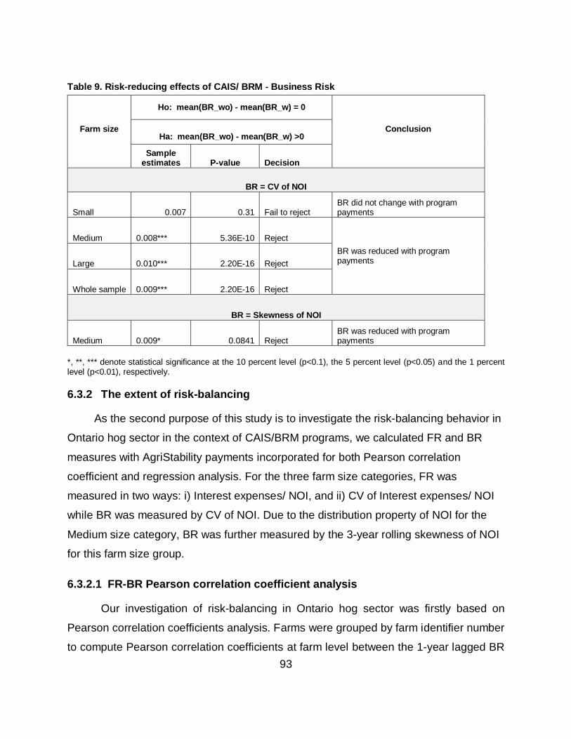
93

Table 9. Risk-reducing effects of CAIS/ BRM - Business Risk

*, **, *** denote statistical significance at the 10 percent level (p<0.1), the 5 percent level (p<0.05) and the 1 percent level (p<0.01), respectively.

6.3.2 The extent of risk-balancing

As the second purpose of this study is to investigate the risk-balancing behavior in

Ontario hog sector in the context of CAIS/BRM programs, we calculated FR and BR

measures with AgriStability payments incorporated for both Pearson correlation

coefficient and regression analysis. For the three farm size categories, FR was

measured in two ways: i) Interest expenses/ NOI, and ii) CV of Interest expenses/ NOI

while BR was measured by CV of NOI. Due to the distribution property of NOI for the

Medium size category, BR was further measured by the 3-year rolling skewness of NOI

for this farm size group.

6.3.2.1 FR-BR Pearson correlation coefficient analysis

Our investigation of risk-balancing in Ontario hog sector was firstly based on

Pearson correlation coefficients analysis. Farms were grouped by farm identifier number

to compute Pearson correlation coefficients at farm level between the 1-year lagged BR

Farm size

Ho: mean(BR_wo) - mean(BR_w) = 0

Conclusion Ha: mean(BR_wo) - mean(BR_w) >0

Sample estimates P-value Decision

BR = CV of NOI

Small 0.007 0.31 Fail to reject BR did not change with program payments

Medium 0.008*** 5.36E-10 Reject

BR was reduced with program payments Large 0.010*** 2.20E-16 Reject

Whole sample 0.009*** 2.20E-16 Reject

BR = Skewness of NOI

Medium 0.009* 0.0841 Reject BR was reduced with program payments

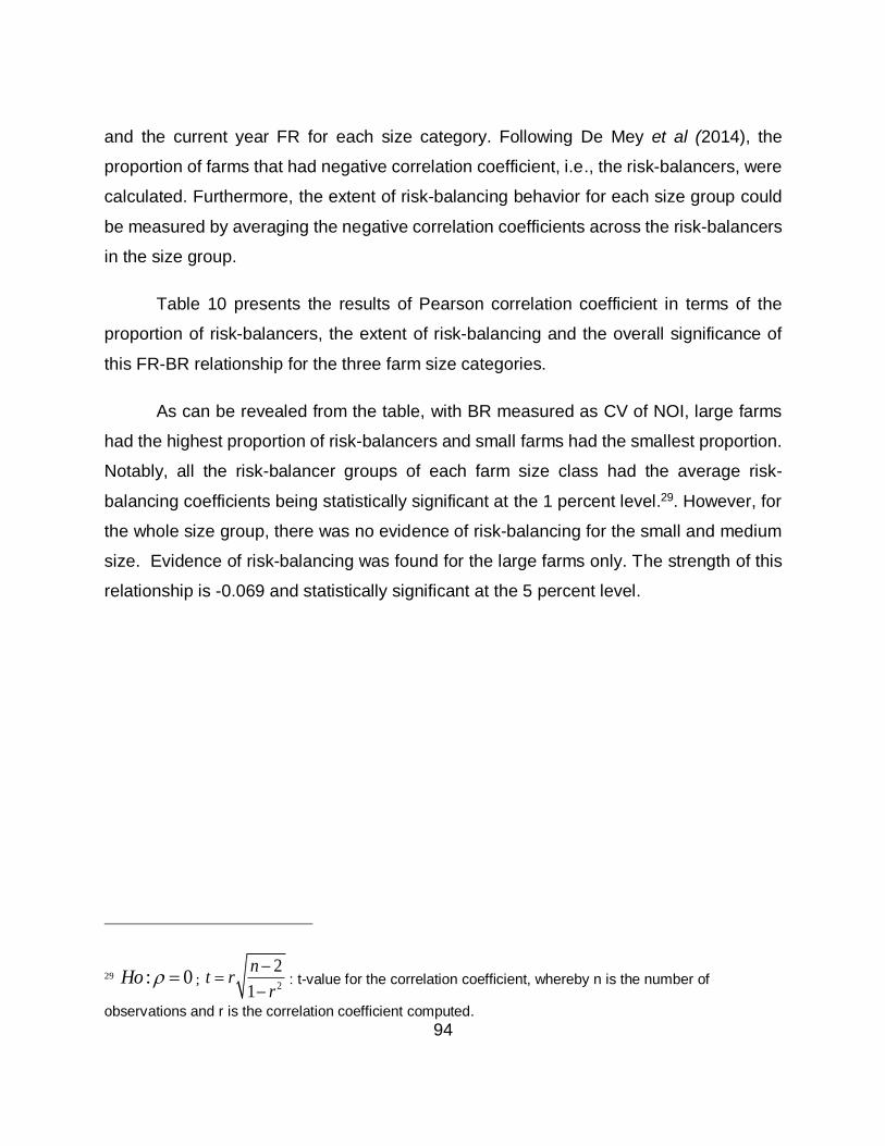
94

and the current year FR for each size category. Following De Mey et al (2014), the

proportion of farms that had negative correlation coefficient, i.e., the risk-balancers, were

calculated. Furthermore, the extent of risk-balancing behavior for each size group could

be measured by averaging the negative correlation coefficients across the risk-balancers

in the size group.

Table 10 presents the results of Pearson correlation coefficient in terms of the

proportion of risk-balancers, the extent of risk-balancing and the overall significance of

this FR-BR relationship for the three farm size categories.

As can be revealed from the table, with BR measured as CV of NOI, large farms

had the highest proportion of risk-balancers and small farms had the smallest proportion.

Notably, all the risk-balancer groups of each farm size class had the average risk-

balancing coefficients being statistically significant at the 1 percent level.29. However, for

the whole size group, there was no evidence of risk-balancing for the small and medium

size. Evidence of risk-balancing was found for the large farms only. The strength of this

relationship is -0.069 and statistically significant at the 5 percent level.

29 : 0Ho ; 2

2

1

nt r

r

: t-value for the correlation coefficient, whereby n is the number of

observations and r is the correlation coefficient computed.

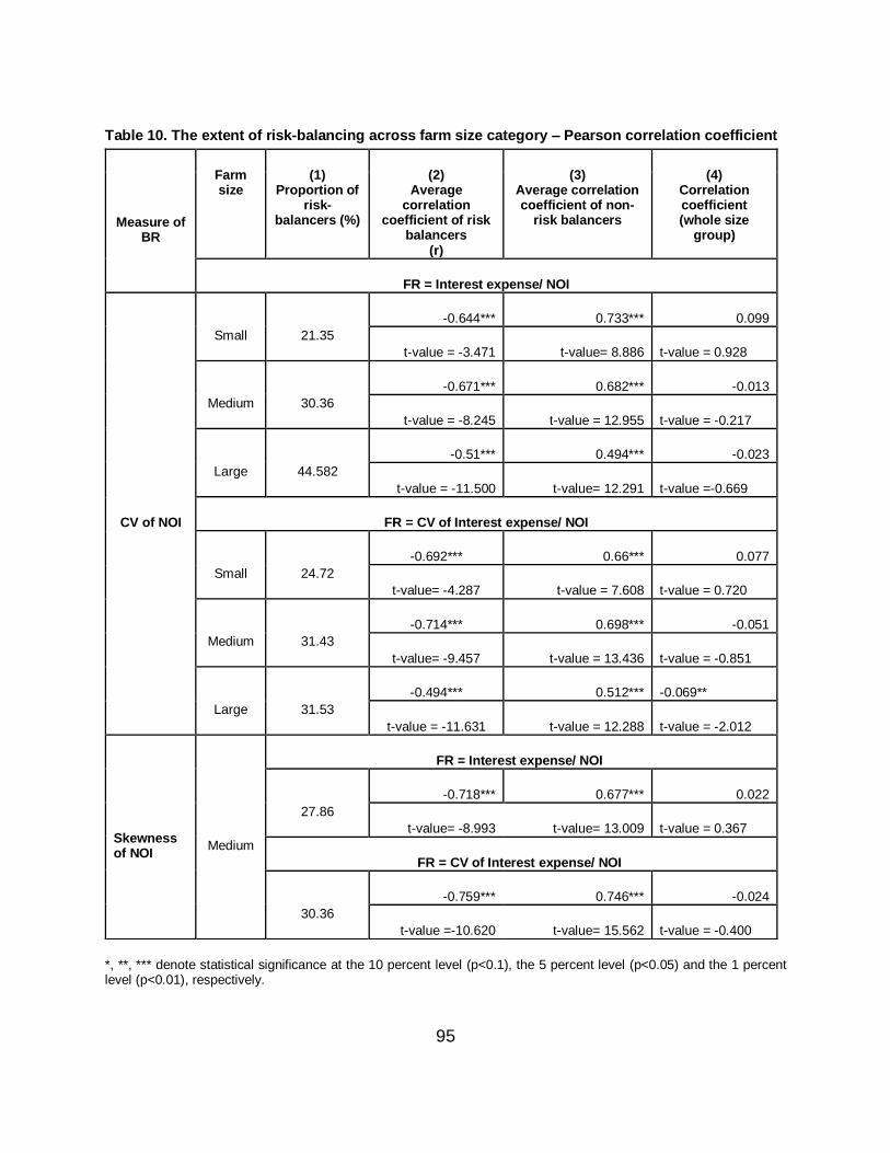
95

Table 10. The extent of risk-balancing across farm size category – Pearson correlation coefficient

*, **, *** denote statistical significance at the 10 percent level (p<0.1), the 5 percent level (p<0.05) and the 1 percent level (p<0.01), respectively.

Measure of BR

Farm size

(1) Proportion of

risk-balancers (%)

(2) Average

correlation coefficient of risk

balancers (r)

(3) Average correlation coefficient of non-

risk balancers

(4) Correlation coefficient (whole size

group)

FR = Interest expense/ NOI

CV of NOI

Small 21.35

-0.644*** 0.733*** 0.099

t-value = -3.471 t-value= 8.886 t-value = 0.928

Medium 30.36

-0.671*** 0.682*** -0.013

t-value = -8.245 t-value = 12.955 t-value = -0.217

Large 44.582

-0.51*** 0.494*** -0.023

t-value = -11.500 t-value= 12.291 t-value =-0.669

FR = CV of Interest expense/ NOI

Small 24.72

-0.692*** 0.66*** 0.077

t-value= -4.287 t-value = 7.608 t-value = 0.720

Medium 31.43

-0.714*** 0.698*** -0.051

t-value= -9.457 t-value = 13.436 t-value = -0.851

Large 31.53

-0.494*** 0.512*** -0.069**

t-value = -11.631 t-value = 12.288 t-value = -2.012

Skewness of NOI

Medium

FR = Interest expense/ NOI

27.86

-0.718*** 0.677*** 0.022

t-value= -8.993 t-value= 13.009 t-value = 0.367

FR = CV of Interest expense/ NOI

30.36

-0.759*** 0.746*** -0.024

t-value =-10.620 t-value= 15.562 t-value = -0.400

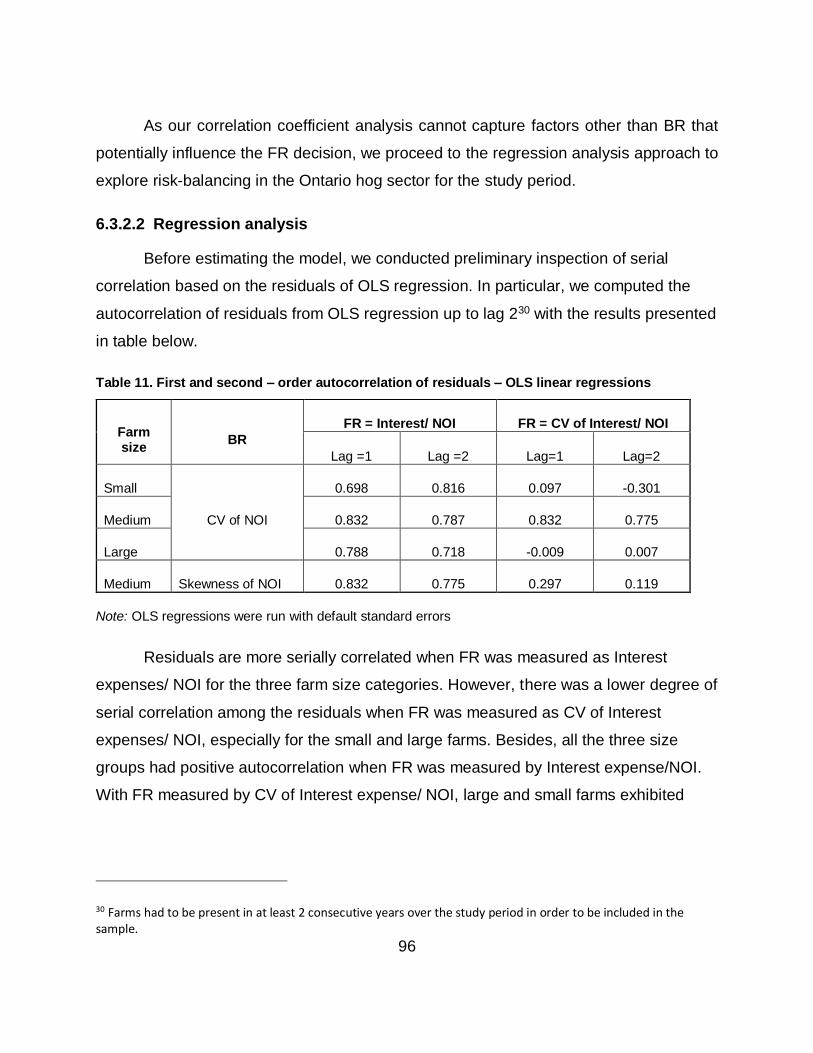
96

As our correlation coefficient analysis cannot capture factors other than BR that

potentially influence the FR decision, we proceed to the regression analysis approach to

explore risk-balancing in the Ontario hog sector for the study period.

6.3.2.2 Regression analysis

Before estimating the model, we conducted preliminary inspection of serial

correlation based on the residuals of OLS regression. In particular, we computed the

autocorrelation of residuals from OLS regression up to lag 230 with the results presented

in table below.

Table 11. First and second – order autocorrelation of residuals – OLS linear regressions

Note: OLS regressions were run with default standard errors

Residuals are more serially correlated when FR was measured as Interest

expenses/ NOI for the three farm size categories. However, there was a lower degree of

serial correlation among the residuals when FR was measured as CV of Interest

expenses/ NOI, especially for the small and large farms. Besides, all the three size

groups had positive autocorrelation when FR was measured by Interest expense/NOI.

With FR measured by CV of Interest expense/ NOI, large and small farms exhibited

30 Farms had to be present in at least 2 consecutive years over the study period in order to be included in the sample.

Farm size

BR

FR = Interest/ NOI FR = CV of Interest/ NOI

Lag =1 Lag =2 Lag=1 Lag=2

Small

CV of NOI

0.698 0.816 0.097 -0.301

Medium 0.832 0.787 0.832 0.775

Large 0.788 0.718 -0.009 0.007

Medium Skewness of NOI 0.832 0.775 0.297 0.119

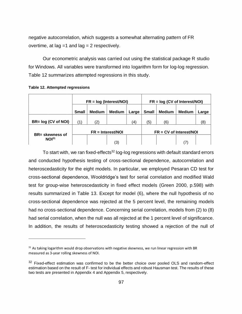
97

negative autocorrelation, which suggests a somewhat alternating pattern of FR

overtime, at lag =1 and lag = 2 respectively.

Our econometric analysis was carried out using the statistical package R studio

for Windows. All variables were transformed into logarithm form for log-log regression.

Table 12 summarizes attempted regressions in this study.

Table 12. Attempted regressions

To start with, we ran fixed-effects32 log-log regressions with default standard errors

and conducted hypothesis testing of cross-sectional dependence, autocorrelation and

heteroscedasticity for the eight models. In particular, we employed Pesaran CD test for

cross-sectional dependence, Wooldridge’s test for serial correlation and modified Wald

test for group-wise heteroscedasticity in fixed effect models (Green 2000, p.598) with

results summarized in Table 13. Except for model (6), where the null hypothesis of no

cross-sectional dependence was rejected at the 5 percent level, the remaining models

had no cross-sectional dependence. Concerning serial correlation, models from (2) to (8)

had serial correlation, when the null was all rejected at the 1 percent level of significance.

In addition, the results of heteroscedasticity testing showed a rejection of the null of

31 As taking logarithm would drop observations with negative skewness, we run linear regression with BR measured as 3-year rolling skewness of NOI.

32 Fixed-effect estimation was confirmed to be the better choice over pooled OLS and random-effect estimation based on the result of F- test for individual effects and robust Hausman test. The results of these two tests are presented in Appendix 4 and Appendix 5, respectively.

FR = log (Interest/NOI) FR = log (CV of Interest/NOI)

Small Medium Medium Large Small Medium Medium Large

BR= log (CV of NOI) (1) (2) (4) (5) (6) (8)

BR= skewness of NOI31

FR = Interest/NOI FR = CV of Interest/NOI

(3) (7)

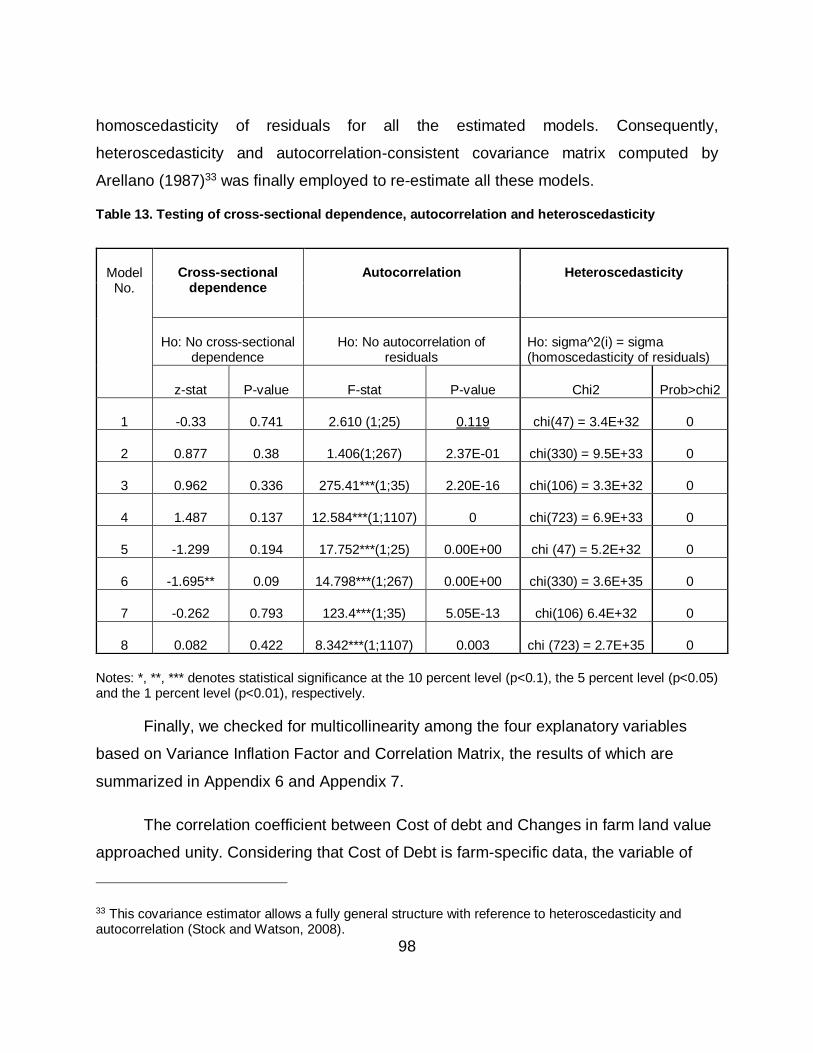
98

homoscedasticity of residuals for all the estimated models. Consequently,

heteroscedasticity and autocorrelation-consistent covariance matrix computed by

Arellano (1987)33 was finally employed to re-estimate all these models.

Table 13. Testing of cross-sectional dependence, autocorrelation and heteroscedasticity

Notes: *, **, *** denotes statistical significance at the 10 percent level (p<0.1), the 5 percent level (p<0.05) and the 1 percent level (p<0.01), respectively.

Finally, we checked for multicollinearity among the four explanatory variables

based on Variance Inflation Factor and Correlation Matrix, the results of which are

summarized in Appendix 6 and Appendix 7.

The correlation coefficient between Cost of debt and Changes in farm land value

approached unity. Considering that Cost of Debt is farm-specific data, the variable of

33 This covariance estimator allows a fully general structure with reference to heteroscedasticity and autocorrelation (Stock and Watson, 2008).

Model No.

Cross-sectional dependence

Autocorrelation Heteroscedasticity

Ho: No cross-sectional dependence

Ho: No autocorrelation of residuals

Ho: sigma^2(i) = sigma (homoscedasticity of residuals)

z-stat P-value F-stat P-value Chi2 Prob>chi2

1 -0.33 0.741 2.610 (1;25) 0.119 chi(47) = 3.4E+32 0

2 0.877 0.38 1.406(1;267) 2.37E-01 chi(330) = 9.5E+33 0

3 0.962 0.336 275.41***(1;35) 2.20E-16 chi(106) = 3.3E+32 0

4 1.487 0.137 12.584***(1;1107) 0 chi(723) = 6.9E+33 0

5 -1.299 0.194 17.752***(1;25) 0.00E+00 chi (47) = 5.2E+32 0

6 -1.695** 0.09 14.798***(1;267) 0.00E+00 chi(330) = 3.6E+35 0

7 -0.262 0.793 123.4***(1;35) 5.05E-13 chi(106) 6.4E+32 0

8 0.082 0.422 8.342***(1;1107) 0.003 chi (723) = 2.7E+35 0

99

changes in farmland value was removed from the regression. Consequently, our model

estimation consists of 3 explanatory variables.

Estimation results for the entire sample34 are presented in Table 14. There is

evidence of risk-balancing behavior for the entire sample of Ontario hog sector during

the study period with FR measured as CV of Interest expenses to NOI ratio. On

average, a one percent reduction in previous year’s BR level was associated with an

increase of 0.06 percent in the current year FR, all other factors remaining unchanged

(Table 14).

We proceeded to estimate the model separately for each farm size category.

Estimation results with BR measured as CV of NOI are presented in Table 15 for

interpretation.

34 BR measured as skewness of NOI was computed for medium farms only. Therefore, BR measured as

CV of NOI was used for whole sample regression

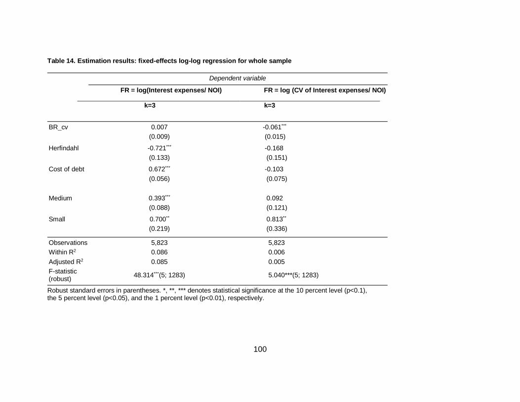
100

Table 14. Estimation results: fixed-effects log-log regression for whole sample

Dependent variable

FR = log(Interest expenses/ NOI) k=3

FR = log (CV of Interest expenses/ NOI) k=3

BR_cv 0.007 -0.061*** (0.009) (0.015)

Herfindahl -0.721*** -0.168 (0.133) (0.151)

Cost of debt 0.672*** -0.103 (0.056) (0.075)

Medium 0.393*** 0.092 (0.088) (0.121)

Small 0.700** 0.813** (0.219) (0.336)

Observations 5,823 5,823

Within R2 0.086 0.006

Adjusted R2 0.085 0.005

F-statistic (robust)

48.314***(5; 1283) 5.040***(5; 1283)

Robust standard errors in parentheses. *, **, *** denotes statistical significance at the 10 percent level (p<0.1), the 5 percent level (p<0.05), and the 1 percent level (p<0.01), respectively.

101

There was evidence of risk-balancing for medium (model 6) and large farms

(model 8) in the Ontario hog sector during the study period, with BR measured as CV of

NOI and FR as CV of Interest expenses/ NOI. Specifically, BR has coefficient estimate

valued -0.087 for medium farms and -0.06 for large farms, statistically significant at the 5

percent and 1 percent level, respectively. This indicates that medium and large farms in

Ontario hog sector made strategic FR adjustments in line with the risk-balancing

hypothesis during the study period. On average, 1 percent reduction in the previous year’s

BR level was associated with 0.087 percent increase in current year FR for medium farms

and 0.06 percent increase in FR level for large farms, ceteris paribus.

Herfindahl index had the expected negative sign for its coefficient for medium

farms, with both FR measurements and for large farms with FR-CV measure. In particular,

for medium farms, a 1 percent reduction in Herfindahl index, i.e., farms becoming more

diversified, would be associated with 0.926 percent increase in the FR level taken and

this effect is significant at the 5 percent level. For large farms, the magnitude of FR-HI

relationship is approximately 0.75 percent. This indicates that for medium and large farms

in Ontario hog sector, the more diversified farms are, the more FR farms would take and

vice versa. In this light, farm diversification might have been used as an alternative risk

management strategy for large farms. Another possibility was that diversification of farm

operations might have helped farms of this size class to have a better credit ratings with

large borrowing, and thus, incurred higher financial risk.

Cost of Debt exhibits the expected negative sign for large farms, when FR was

measured as CV of the Interest expenses to NOI ratio. This suggests that for large farms,

a higher cost of debts in the previous year would be associated with a lower variation

degree of the Interest expense/ NOI ratio and vice versa. On average, a 1 percent

increase in last year’s cost of debt would be associated with a 0.156 percent reduction in

the variation of the Interest expenses/ NOI ratio, ceteris paribus. And this effect is

statistically significant at the 10 percent level. However, the situation was reverse when

FR was measured by the magnitude of the Interest expense to NOI ratio. For both medium

102

and large farms, a 1 percent increase in historical cost of debt would be associated with

an increase of 0.418 percent and 0.738 percent in the magnitude of Interest expense/

NOI in the current year for medium and large farms, respectively. One possible

explanation is that farms faced tough financial situations and had great demand for

borrowing to finance their business operations, taking into account the period of adversity

for the hog sector between 2006 and 2011. As a possible result, historical costs of debt

may not be negatively related to the current period’s FR decisions.

For Small size category, there was no evidence of risk-balancing behavior, with

both FR measures. This is understandable as small farms do not have the same

accessibility to credit compared with medium and large farms. However, we can hardly

make a conclusive statement for this farm size category as the number of observations

retained in the regression is quite low relative to the number of small farms in the sample.

The coefficient of determination 2R is quite low for the estimated models.

Nevertheless, this would not be considered as a serious issue since the purpose of this

study is not to predict, but to explore the extent of the FR-BR relationship.

Estimation results of linear regressions are summarized in Appendix 8. It is worth

noting that linear regressions were run with both BR measures, as CV of NOI and as

skewness of NOI for medium farms. Overall, no evidence of risk-balancing was found for

the three farm size categories in the case of linear regression (Appendix 8).

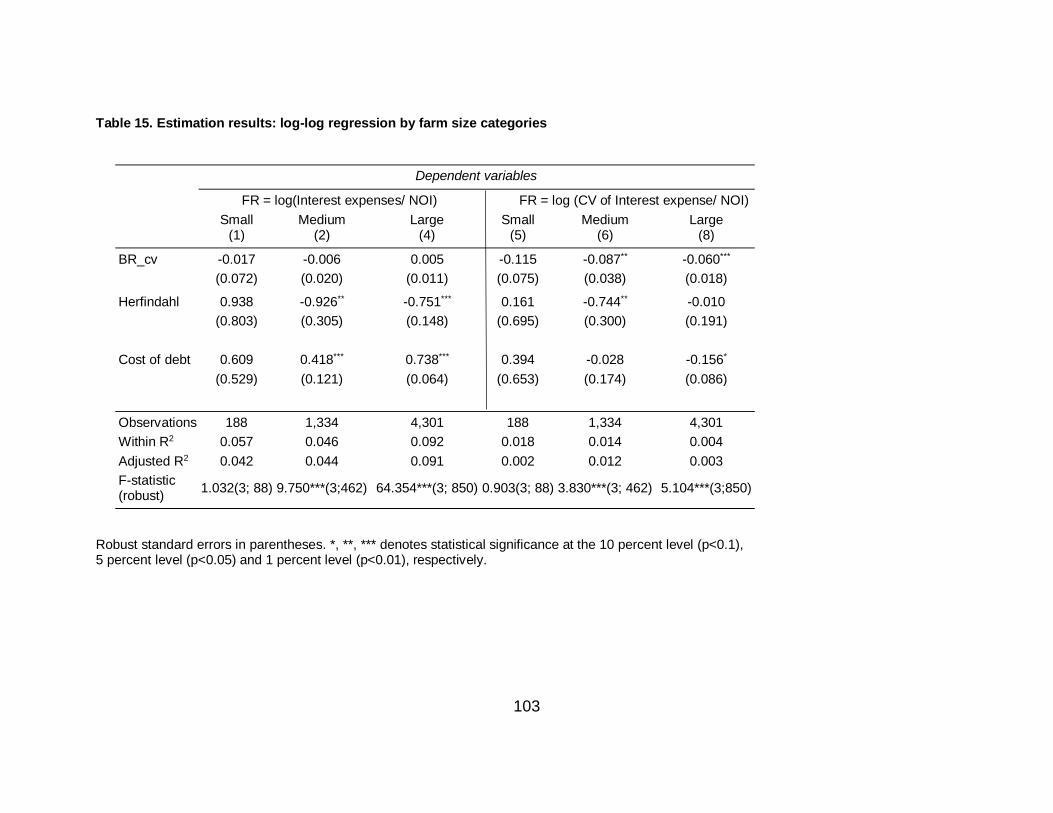
103

Table 15. Estimation results: log-log regression by farm size categories

Robust standard errors in parentheses. *, **, *** denotes statistical significance at the 10 percent level (p<0.1), 5 percent level (p<0.05) and 1 percent level (p<0.01), respectively.

Dependent variables

FR = log(Interest expenses/ NOI) FR = log (CV of Interest expense/ NOI)

Small (1)

Medium (2)

Large (4)

Small (5)

Medium (6)

Large (8)

BR_cv -0.017 -0.006 0.005 -0.115 -0.087** -0.060*** (0.072) (0.020) (0.011) (0.075) (0.038) (0.018)

Herfindahl 0.938 -0.926** -0.751*** 0.161 -0.744** -0.010 (0.803) (0.305) (0.148) (0.695) (0.300) (0.191)

Cost of debt 0.609 0.418*** 0.738*** 0.394 -0.028 -0.156* (0.529) (0.121) (0.064) (0.653) (0.174) (0.086)

Observations 188 1,334 4,301 188 1,334 4,301

Within R2 0.057 0.046 0.092 0.018 0.014 0.004

Adjusted R2 0.042 0.044 0.091 0.002 0.012 0.003


1.032(3; 88) 9.750***(3;462) 64.354***(3; 850) 0.903(3; 88) 3.830***(3; 462) 5.104***(3;850)

104

6.4 Chapter summary

This chapter presents empirical approaches and corresponding results in

examining the effectiveness of CAIS/BRM programs and the extent of risk-balancing

behavior in Ontario hog sector during the 2003-2014 period.

Our key findings were that with BR measured as CV of NOI, the programs were

effective in reducing BR for large and medium farms, but not for small farms. Especially

for medium farms, the program payments reduced the variations of NOI around its

mean as well as affected its two tails of distribution, i.e., the infrequent but extreme

losses or gains of NOI.

Concerning the extent of risk-balancing, evidence of risk-balancing was found for

large and medium farms in Ontario hog sector but not for small farms.

105

7 CHAPTER 7: CONCLUSION

7.1 Research summary

Agri-food sectors in Canada are supported through safety net programs. Over time

the safety-net programs in Canada have evolved from a commodity-based to whole-farm

based program. The focus also changed from price stabilization to income stabilization.

CAIS/BRM programs were designed to help producers reduce BR by mitigating negative

income shocks and reducing income variability. However, according to the risk-balancing

hypothesis, farms may take more FR in response to a reduction in BR as a result of

program payments. If we find evidence of such behavior, risk-reduction efforts of

CAIS/BRM programs may not generate intended outcomes and therefore, may jeopardize

the economic stability and viability of the Canadian agri-food sectors.

The literature on risk-balancing indicates that there are different ways to measure

BR in agricultural sectors. Yet there is no definitive way of measuring BR that could

capture the magnitude of the infrequent but extreme losses while accounting for the

skewness property of its distribution. On the other hand, while a number of papers use

pairwise correlation coefficient to measure the extent of risk-balancing in agricultural

sectors in Canada, some other studies employed regression analysis to account for other

factors that may have an impact on the FR decisions. Nevertheless, whether this behavior

differs among farms of different size categories has not been fully investigated.

Concerning the analytical framework, our comparative statistic analysis further

confirms the risk-balancing model introduced by Gabriel and Barker (1980) and Collins

(1985). The latter maintains that for the risk-balancing hypothesis to hold, proprietor is

assumed to be an expected utility maximizer with a risk-averse attitude. Besides, potential

factors other than BR that may induce a change in FR decision should also be included

in the risk-balancing model. Furthermore, in order to have a more accurate measure of

BR, Crop Insurance should be included in the model in the calculation of BR since both

risk-premium and Crop Insurance indemnities affect the distribution of the farm profit. Our

analytical framework demonstrates this.

106

Regarding our empirical analysis, using OFID tax-filing data over the 2003-2014

period, we investigated the risk-reducing effects of AgriStability payments under CAIS/

BRM programs on the Ontario hog sector and estimated the extent of risk-balancing in

the sector afterwards. Concerning the effectiveness of CAIS/BRM programs, paired t-test

was employed to test for the statistical significance of the mean difference of BR without

and with program payments. The result was that CAIS/AgriStability payments were

effective in reducing BR for medium and large farms. However, there was no risk-reducing

effect for the small hog farms.

Given the effectiveness of CAIS/AgriStability payments, we subsequently

estimated the extent of risk-balancing in the sector. Specifically, we first followed the

correlation coefficient approach proposed by Escalante and Barry (2003) and

subsequently estimated the strength of risk-balancing by using the regression analysis

approach employed by De Mey et al (2014).

For our key findings, our correlation coefficient analysis points out that out of the

three size categories, large farms had the highest proportion of risk-balancers and small

size farms had the smallest. In addition, the evidence of risk-balancing was found for the

large farms, with BR measured as CV of NOI and FR measured as CV of Interest

expenses/ NOI. The strength of this inverse relationship is -0.069, significant at the 5

percent level of significance.

Controlling for other determinants of FR, our log-log fixed-effects regression

provides evidence in favor of risk-balancing for Ontario hog farms as a whole, with FR

measured as CV of Interest expenses/ NOI. Taking into account the heterogeneity of the

sample as revealed by our descriptive statistics, we run the log-log regression separately

for each farm size category.

Our findings confirmed evidence of risk-balancing for medium and large farms with

BR measured as CV of NOI and FR as CV of Interest expenses to NOI ratio. On average,

1 percent decrease in the previous year’s BR level was associated with 0.087 percent

107

increase in current year FR for medium farms and 0.067 percent increase in FR level for

large farms, all other factors remaining unchanged. Consistent with our correlation

coefficient analysis, our regression results found no evidence of risk-balancing for the

small farm size categories. But again, statement on the evidence of risk-balancing for this

farm size is not as conclusive as those for medium and large farms.

In general, our empirical results substantiate previous studies by providing

empirical evidence of: i) the risk-reduction effects of AgriStability payments under CAIS/

BRM programs; ii) risk-balancing in Ontario hog sector for the large and medium farm

size categories during the study period. In view of the fact that findings from the study can

set light on the FR-BR relationship in the Ontario hog sector, especially with farm-size

group specific results, our research objective was realized and our research questions

were answered.

7.2 Policy implications

While CAIS/ BRM programs were designed to address BR for farms of all size

categories, our empirical results indicate that AgriStability payments under the programs

reduced BR for medium and large farms, but not for small farms. On the other hand, our

descriptive statistics as well as our visual inspection of risk measures across farm size

groups reveal that small farms faced a greater degree of BR compared with the medium

and large farm sizes during the study period. If income stabilization is an important goal

of these programs, this goal has been achieved for the medium and large farm size

categories. As these two farm size classes account for approximately 95 percent of the

number of hog farms in Ontario, this goal realization is meaningful for the long-run

viability of the Ontario hog sector.

Furthermore, our empirical findings provide evidence of risk-balancing for medium

and large farms during the study period 2003-2014. This means that as CAIS/ BRM

programs reduced BR for medium and large farms, these farms incurred more FR as a

result of risk-balancing. Nevertheless, as long as the reduction in BR level was not more

than offset by an increase in FR level, the viability of the programs would not be

108

questioned. This was proved to be the case for Ontario hog sector, as our formal test for

the effectiveness of CAIS/ BRM programs revealed that the total risk that medium and

large farms faced were also reduced during the study period. In this light, the presence

of risk-balancing behavior found for the medium and large farms in the Ontario hog

sector do not seem to pose any threat to the long-run viability of CAIS/ BRM programs

and the sustainability of the hog sector in Ontario.

7.3 Contributions of the study

Our study provides the first empirical evidence of risk-balancing in Ontario hog

sector for the 2003-2014 period. Apart from bridging this gap, the research also

contributes to the risk-balancing literature by making an attempt to measure BR as rolling

skewness of NOI. This skewness measurement relaxes the underlying assumption of the

Coefficient of Variation measurement that the variable used for computing BR measure

is normally distributed. Furthermore, believing that variability implies uncertainty and risk

in itself, an attempt was made to employ CV of the Interest expenses – NOI ratio as an

alternative way of measuring FR. Last but not least, for theoretical side, Crop Insurance

was firstly incorporated into the analytical framework by Collins’ (1985) to model risk-

balancing so as to provide a more accurate measurement of BR.

One of the limitations of the study lies in its failure to incorporate Crop Insurance

payments into empirical analysis due to data constraint. As corroborated in our theoretical

framework, BR might be overestimated and thus, leading to under-estimation of FR in the

presence of risk-balancing. However, it would not be a serious issue as our empirical

analysis was on the hog sector, for which Crop Insurance is not as important as it is for

the field crop sector.

7.4 Suggestions for further research

Given the evidence of risk-balancing in Ontario hog sector, future research could

look at the interactions between risk balancing and other risk-management strategies,

e.g., farm diversification or strategies to manage off-farm income. As contended by

109

Wauters (2012), one potential significant risk management strategy could be household

buffering such as off-farm income.

Another interesting avenue for further research could be to incorporate Crop

Insurance into empirical analysis for a more accurate BR measure, especially for field

crops farms where Crop Insurance is important. Taking into account Crop Insurance

purchase, future research could extend the present analysis by exploring the

relationship between Crop Insurance and BRM programs and answering some relevant

pending questions, i.e., Is Crop Insurance an alternative strategy to BRM payments?

And as such, do BRM programs reduce farmers’ incentives to purchase Crop

Insurance?

On methodological grounds, future risk-balancing research under BRM programs

could hopefully make good use of a better dataset to further look at alternative

definitions of BR so as to replicate the Program Margin formulated under AgriStability

payment scheme. In this way of definition, BR would better reflect the risk-reducing

effects of the programs. Also, incorporating risk-attitude in line with the utility-centric risk

balancing models by Collins (1985) and Featherstone et al (1988) could be another

option for further consideration. Finally, future work could extend present analysis to

further measure BR so as to both capture the skewness property of the margin variable

and the magnitude of its left tail. In this light, the magnitude of the downside risk can be

assessed in relation to the upside risk.

110

REFERENCES

Agricorp.2007. Canadian Agricultural Income Stabilization Handbook. Retrieved from: http://www.agricorp.com/SiteCollectionDocuments/AgriStability-Handbook-en.pdf

Agriculture and Agri-Food Canada. 2005. Agricultural Policy Framework: Federal, Provincial, Territorial Programs. Retrieved from: http://publications.gc.ca/collections/Collection/A34-3-2005E.pdf

Agriculture and Agri-Food Canada. 2011. AgriStability Program Handbook. Retrieved from: https://www5.agr.gc.ca/eng/?id=1294427843421

Agriculture and Agri-Food Canada. 2012. Growing Forward 2. Retrieved from: http://publications.gc.ca/collections/collection_2012/parl/XC12-1-411-01-eng.pdf

Agriculture and Agri-Food Canada. 2017. Growing Forward 2. http://www.agr.gc.ca/eng/about-us/key departmental-initiatives/growing-forward-2/?id=1294780620963 (accessed: May 26, 2017)

Anton, J., S. Kimura and R. Martini. 2011. “Risk Management in Agriculture in Canada”, OECD Food, Agriculture and Fisheries Paperss, No. 40. OECD Publishing, Paris. http://dx.doi.org/10.1787/5kgj0d6189wg-en

Arellano, M. 1987. Computing Robust Standard Errors for Within-Group Estimators. Oxford Bulletin of Economics and Statistics. 49(4): 431-34.

Barges, Alexander. The Effect of Capital Structure on the Cost of Capital. Englewood Cliffs, N. J.: Prentice-hall, 1963.

Brisson, Y. 2015.The changing face of the Canadian hog industry. In Canadian Agriculture At a glance (96-325-x-No.005) [updated: Nov 30, 2015, accessed: Jun 16, 2018] https://www150.statcan.gc.ca/n1/pub/96-325-x/2014001/article/14027-eng.htm

Cabas, J. H., A. J. Leiva and A. Weersink.2008. Modeling exit and entry of farmers in a crop insurance program. Agricultural and Resource Economics Review 37 (1): 92-105.

Canadian Hog Council. No Date. Hog statistics at a glance. http://www.cpc-ccp.com/hog-statistics-at-a-glance (accessed: Jun 16, 2018)

Collins, R. A. 1985. Expected utility, debt-equity structure, and risk balancing. American Journal of Agricultural Economics 67 (3): 627-629.

Escalante, C. L. and P. J. Barry. 2001. Risk balancing in an integrated farm risk management plan. Journal of Agricultural and Applied Economics 33(3): 413-430.

Escalante, C. L. and P. J. Barry. 2003. Determinants of the strength of strategic adjustments in farm capital structure. Journal of Agricultural and Applied Economics 35 (1): 67-78.

Farm Credit Canada. 2017. Farmland values report – historic values. Available at: https://www.fcc-fac.ca/fcc/about-fcc/reports/2017-farmland-values-historic-e.pdf (accessed: April 09, 2018)

http://www.agricorp.com/SiteCollectionDocuments/AgriStability-Handbook-en.pdf

https://www5.agr.gc.ca/eng/?id=1294427843421

http://www.agr.gc.ca/eng/about-us/key%09%09%20departmental-initiatives/growing-forward-2/?id=1294780620963

http://www.agr.gc.ca/eng/about-us/key%09%09%20departmental-initiatives/growing-forward-2/?id=1294780620963

http://dx.doi.org/10.1787/5kgj0d6189wg-en

https://www150.statcan.gc.ca/n1/pub/96-325-x/2014001/article/14027-eng.htm

http://www.cpc-ccp.com/hog-statistics-at-a-

https://www.fcc-fac.ca/fcc/about-%09fcc/reports/2017-farmland-values-historic-e.pdf

111

Featherstone, A. M., C. B. Moss, T. G. Baker and P. V. Preckel. 1988. The theoretical effects of farm policies on optimal leverage and the probability of equity loss. American Journal of Agricultural Economics 70 (3): 572-579.

Gabriel, S. C. and C. B. Baker. 1980. Concepts of business and financial risk. American Journal of Agricultural Economics 62 (3): 560-564.

Greene, W.H. 2000. Econometric analysis. New Jersey, NJ: Prentice Hall

Ifft, J. E., T. Kuethe and M. Morehart. 2015. Does federal crop insurance lead to higher farm debt use? Evidence from the Agricultural Resource Management Survey (ARMS). Agricultural Financial Review 75 (3): 349-367.

Jeffrey, S. R., D. E. Trautman and J. R. Unterschultz. 2017. Canadian Agricultural Business Risk Management Programs: Implications for Farm Wealth and Environmental Stewardship. Canadian

Journal of Agricultural Economics/Revue Canadienne d’agroeconomie. 65 (4): 543-565.

Mey, Y. D, F. V. Winsen, M. Vancauteren, L. Lauwers, S. V. Passel. 2014. Farm-level evidence on risk balancing behavior in the EU-15. Agricultural Finance Review 74 (1):17-37.

Ontario Ministry of Agriculture, Food and Rural Affairs. 2014. Ontario Farm Income Database.

Ontario Ministry of Agriculture, Food and Rural Affairs. 2016. Farm, Rural, Food Processing and Fiber Indicators, Ontario, 2002-2014. http://www.omafra.gov.on.ca/english/stats/economy/indicators.htm (accessed: May 30, 2018).

Ontario Ministry of Agriculture, Food and Rural Affairs. 2017. http://www.omafra.gov.on.ca/english/stats/agriculturesummary.htm#commodities (accessed: Jun 16, 2018)

Ontario Ministry of Agriculture, Food and Rural Affairs. 2017. Estimated farrow to finish swine enterprise budget summary-monthly. http://www.omafra.gov.on.ca/english/livestock/swine/news/janfeb10a4.htm (accessed: Jun 16, 2018)

Ontario Ministry of Agriculture, Food and Rural Affairs. 2017. Livestock and poultry statistics: Average prices received by Ontario farmers for slaughter cattle. http://www.omafra.gov.on.ca/english/stats/livestock/price_cattle.htm (accessed: Jun 16, 2018)

Ontario Ministry of Agriculture, Food and Rural Affairs. 2017. Statistical Summary of Ontario Agriculture. Farm statistics 2001, 2006, 2011 and 2016 Census. http://www.omafra.gov.on.ca/english/stats/agriculturesummary.htm (access May 17, 2017)

Schmitz, A. 2010. Agricultural policy, agribusiness, and rent-seeking behavior. University of Toronto Press.

Schmitz, A.2008. Canadian agricultural programs and policy in transition. American Journal of Agricultural Economics 56 (4): 371-391.

Sherrick, B. J., P.J. Barry, P.N. Ellinger and G.D. Schnitkey.2004. Factors influencing farmers' crop insurance decisions. American Journal of Agricultural Economics 86 (1): 103-114.

http://www.omafra.gov.on.ca/english/stats/economy/indicators.htm

http://www.omafra.gov.on.ca/english/stats/agriculturesummary.htm#commodities

http://www.omafra.gov.on.ca/english/livestock/swine/news/janfeb10a4.htm

http://www.omafra.gov.on.ca/english/stats/livestock/price_cattle.htm

http://www.omafra.gov.on.ca/english/stats/agriculturesummary.htm

112

Skees, J. R.1999. Agricultural risk management or income enhancement. Regulation 22 (1): 35-43.

Statistics Canada. 2006. Census of Agriculture, Farm Data and Farm Operator Data, Catalogue No. 95-629-XWE. https://www150.statcan.gc.ca/n1/pub/95-629-x/1/4123812-eng.htm (accessed: May 30, 2018)

Statistics Canada. No Date. CANSIM Table 002-0009: Net farm income (x1000). CANSIM (database) https://www150.statcan.gc.ca/t1/tbl1/en/tv.action?pid=3210005201 (accessed: May 26, 2017)

Statistics Canada. No Date. Table 32-10-0045-01: Farm cash receipts, annual (x1,000). https://www150.statcan.gc.ca/t1/tbl1/en/tv.action?pid=3210004501 (accessed: Jun 16, 2018)

Statistics Canada. No Date. Table 32-10-0155-01: Selected livestock and poultry, historical data. https://www150.statcan.gc.ca/t1/tbl1/en/tv.action?pid=3210015501 (accessed: Jun 16, 2018)

Statistics Canada. No Date. Table 32-10-0407-01. Census of Agriculture, tenure of land owned, leased, rented, crop-share, used through other arrangements or used by others every 5 years https://www150.statcan.gc.ca/t1/tbl1/en/tv.action?pid=3210040701 (accessed: Jun 16, 2018)

Statistics Canada. No Date. Table: 32-10-0106-01: Direct payments to agricultural producers (x1,000) https://www150.statcan.gc.ca/t1/tbl1/en/tv.action?pid=3210010601 (accessed: Jun 16, 2018)

Stock, J.H. and M.W.Watson. 2008. Heteroskedasticity – robust standard errors for fixed effect panel data regression. Econometrica 76(1): 155-174.

Turvey, C. G. 2012. Whole farm income insurance. Journal of Risk and Insurance 79 (2): 515-40.

Turvey, C. G. and R. Kong. 2009. Business and financial risks of small farm households in China. China Agricultural Economic Review 1 (2): 155-1872.

Ueza, N., K. Poon, D. Sparling and A. Weersink. 2014b. Farm support payments and risk balancing: Implications for financial riskiness of Canadian farms. Canadian Journal of Agricultural Economics 62 (4): 595-618.

Uzea, F., K. Poon, D. Sparling, and A. Weersink. 2014a. Substitutes versus Complements among Canadian Business Risk Management Programs. Paper presented at 2014 Annual Meeting, July 27-29, 2014, Minneapolis, Minnesota.

Van Arsdell, P. M. Corporation Finance. New York: Ronald Press Co., 1968.

Van Horne, J. C. Fundamentals of Financial Management. Englewood Cliffs, N. J: Prentice – Hall, 1974.

Vercammen, J. 2013. A Partial Adjustment Model of Federal Direct Payments in Canadian Agriculture. Canadian Journal of Agricultural Economics 61(3): 465-485.

Wauters, E. 2012. Farm household risk-balancing: implications for policy. Working paper. Institute for Agricultural and Fisheries Research, Social Sciences Unit, Merelbeke, March.

Wauters, E., de Mey, Y., F. V. Winsen, S.V. Passel, M. Vancauteren, L. Lauwers. 2015. Farm household risk balancing: Implications for policy from an EU perspective. Agricultural Finance Review 75 (4): 450-468.

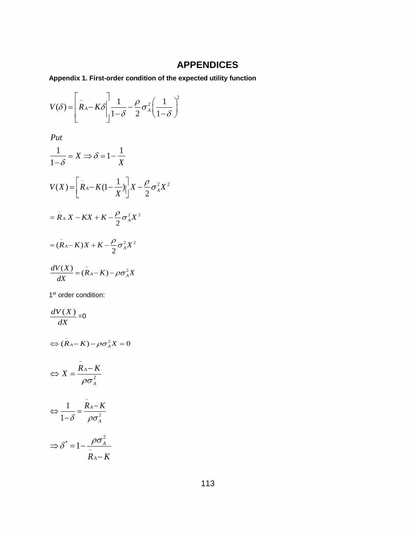
https://www150.statcan.gc.ca/n1/pub/95-629-x/1/4123812-eng.htm

https://www150.statcan.gc.ca/t1/tbl1/en/tv.action?pid=3210005201





113

APPENDICES

Appendix 1. First-order condition of the expected utility function

2

21 1( )

1 2 1A AV R K

1 11

1

Put

XX

2 21( ) (1 )

2A AV X R K X X

X

2 2

2A AR X KX K X

2 2( )2

A AR K X K X

2( )( )A A

dV XR K X

dX

1st order condition:

( )dV X

dX=0

2( ) 0A AR K X

2

A

A

R KX

2

1

1

A

A

R K

2* 1 A

AR K

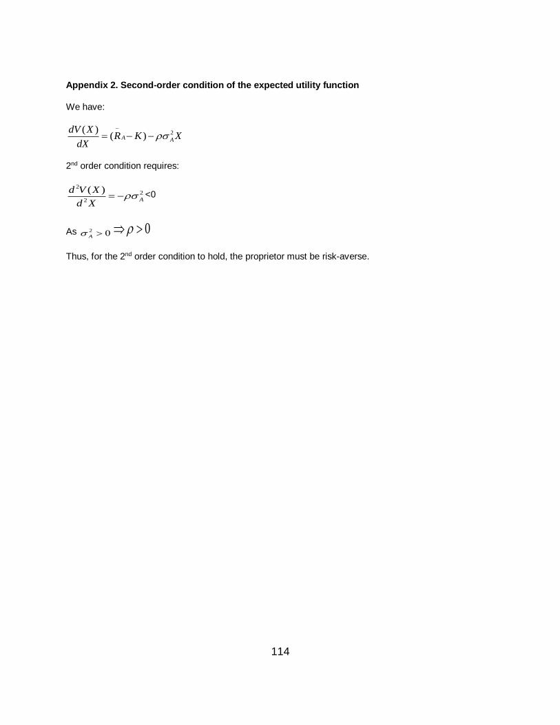
114

Appendix 2. Second-order condition of the expected utility function

We have:

2( )( )A A

dV XR K X

dX

2nd order condition requires:

22

2

( )A

d V X

d X <0

As 2 0A 0

Thus, for the 2nd order condition to hold, the proprietor must be risk-averse.

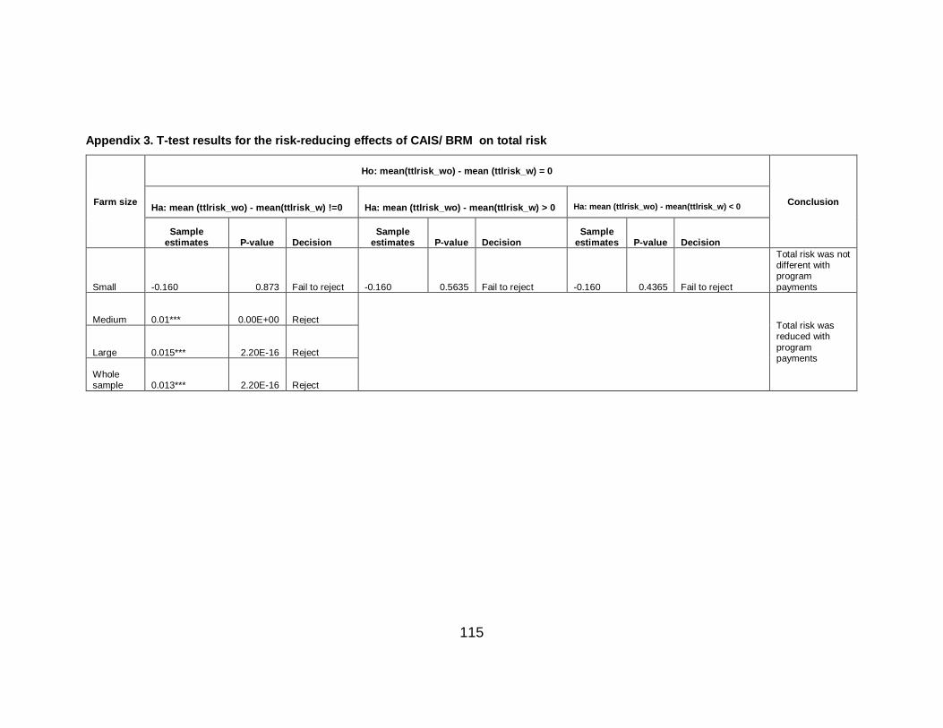
115

Appendix 3. T-test results for the risk-reducing effects of CAIS/ BRM on total risk

Farm size

Ho: mean(ttlrisk_wo) - mean (ttlrisk_w) = 0

Conclusion Ha: mean (ttlrisk_wo) - mean(ttlrisk_w) !=0

Ha: mean (ttlrisk_wo) - mean(ttlrisk_w) > 0

Ha: mean (ttlrisk_wo) - mean(ttlrisk_w) < 0




Small -0.160 0.873 Fail to reject -0.160 0.5635 Fail to reject -0.160 0.4365 Fail to reject

Total risk was not different with program

payments

Medium 0.01*** 0.00E+00 Reject

Total risk was reduced with

program payments

Large 0.015*** 2.20E-16 Reject

Whole sample 0.013*** 2.20E-16 Reject

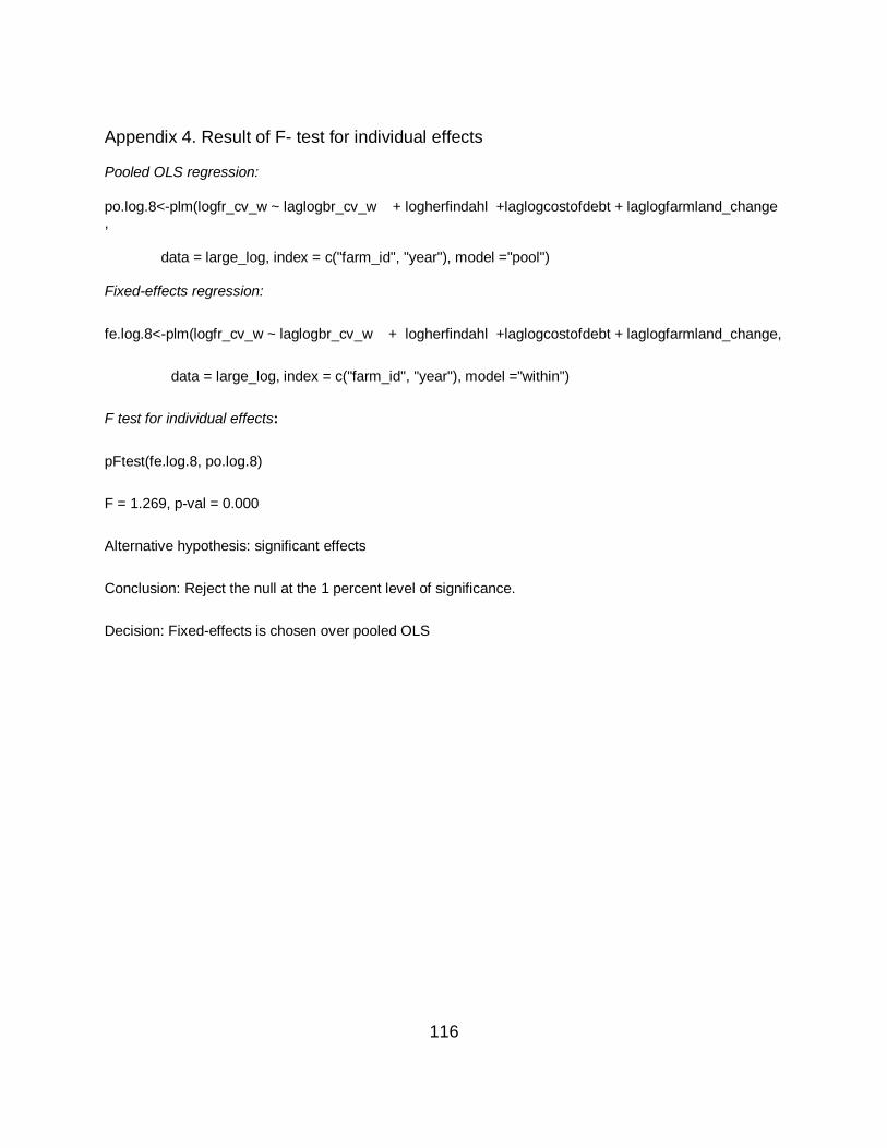
116

Appendix 4. Result of F- test for individual effects

Pooled OLS regression:

po.log.8<-plm(logfr_cv_w ~ laglogbr_cv_w + logherfindahl +laglogcostofdebt + laglogfarmland_change ,

data = large_log, index = c("farm_id", "year"), model ="pool")

Fixed-effects regression:

fe.log.8<-plm(logfr_cv_w ~ laglogbr_cv_w + logherfindahl +laglogcostofdebt + laglogfarmland_change,

data = large_log, index = c("farm_id", "year"), model ="within")

F test for individual effects:

pFtest(fe.log.8, po.log.8)

F = 1.269, p-val = 0.000

Alternative hypothesis: significant effects

Conclusion: Reject the null at the 1 percent level of significance.

Decision: Fixed-effects is chosen over pooled OLS

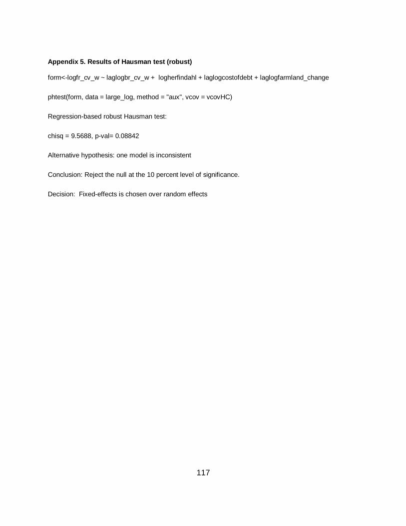
117

Appendix 5. Results of Hausman test (robust)

form<-logfr_cv_w ~ laglogbr_cv_w + logherfindahl + laglogcostofdebt + laglogfarmland_change

phtest(form, data = large_log, method = "aux", vcov = vcovHC)

Regression-based robust Hausman test:

chisq = 9.5688, p-val= 0.08842

Alternative hypothesis: one model is inconsistent

Conclusion: Reject the null at the 10 percent level of significance.

Decision: Fixed-effects is chosen over random effects

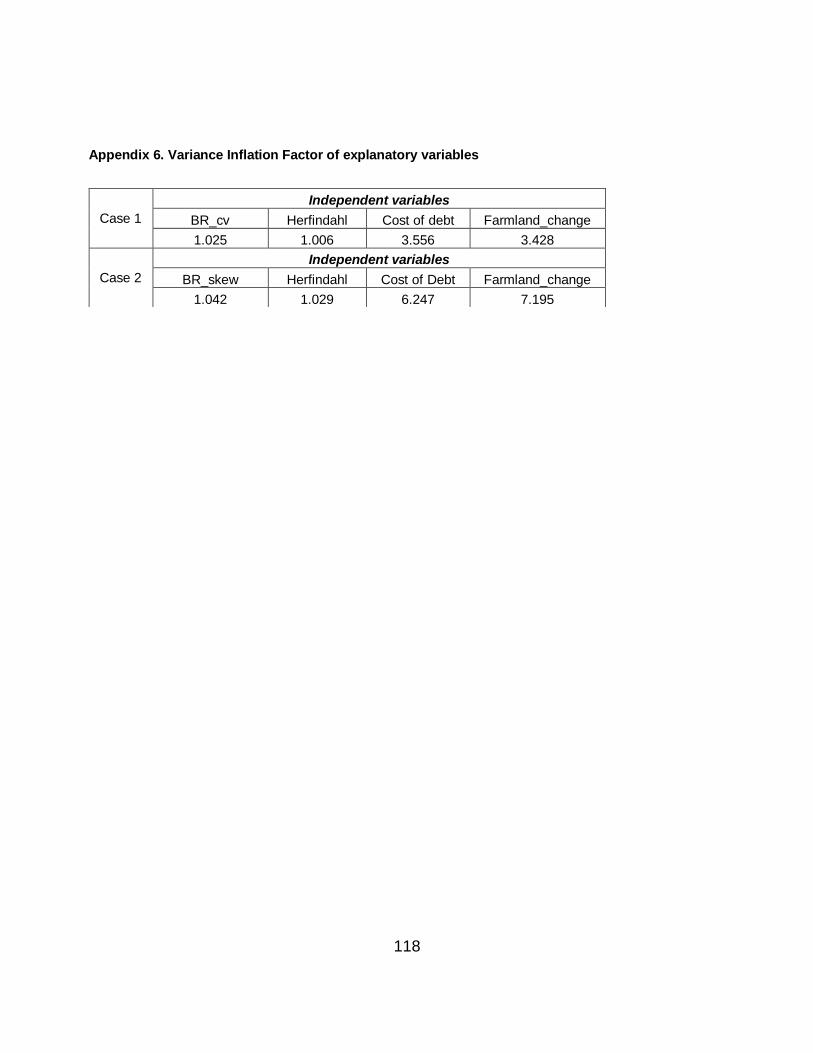
118

Appendix 6. Variance Inflation Factor of explanatory variables

Case 1

Independent variables

BR_cv Herfindahl Cost of debt Farmland_change

1.025 1.006 3.556 3.428

Case 2

Independent variables

BR_skew Herfindahl Cost of Debt Farmland_change

1.042 1.029 6.247 7.195

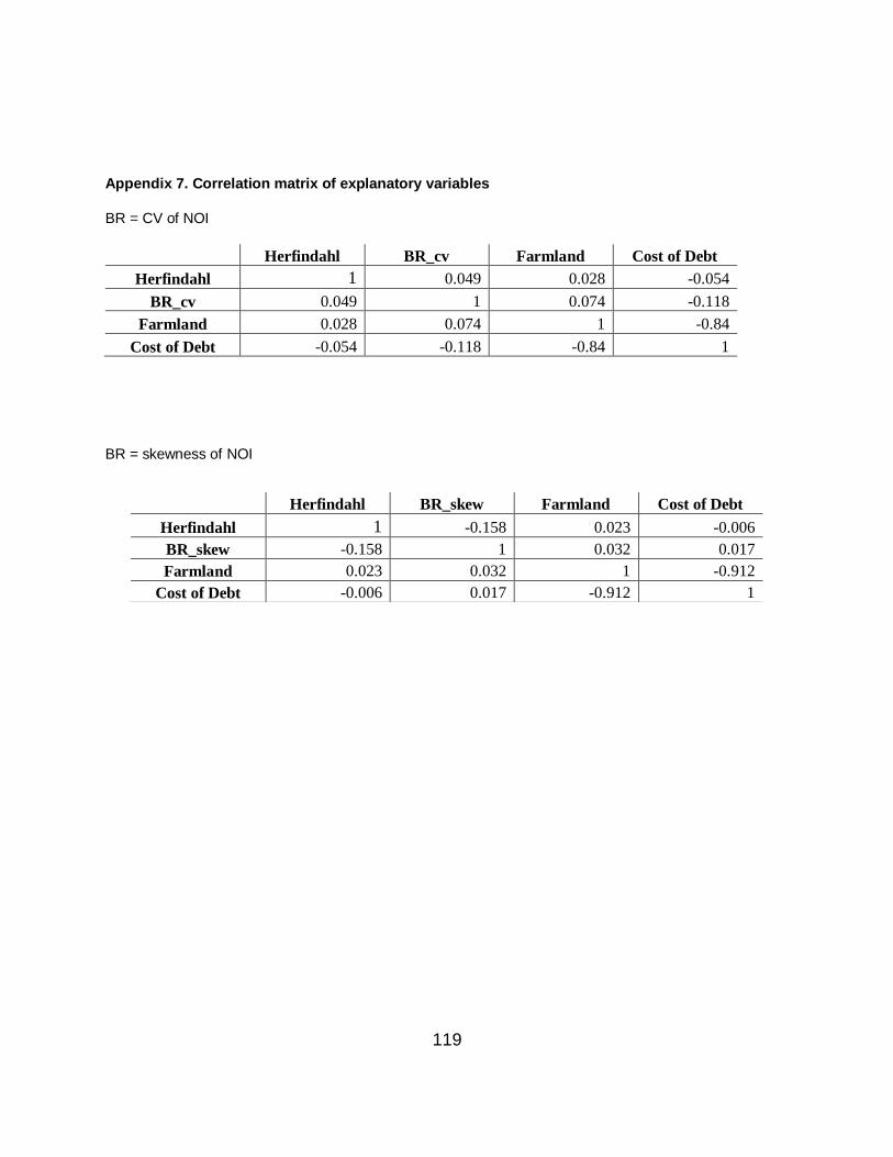
119

Appendix 7. Correlation matrix of explanatory variables

BR = CV of NOI

Herfindahl BR_cv Farmland Cost of Debt

Herfindahl 1 0.049 0.028 -0.054

BR_cv 0.049 1 0.074 -0.118

Farmland 0.028 0.074 1 -0.84

Cost of Debt -0.054 -0.118 -0.84 1

BR = skewness of NOI

Herfindahl BR_skew Farmland Cost of Debt

Herfindahl 1 -0.158 0.023 -0.006

BR_skew -0.158 1 0.032 0.017

Farmland 0.023 0.032 1 -0.912

Cost of Debt -0.006 0.017 -0.912 1

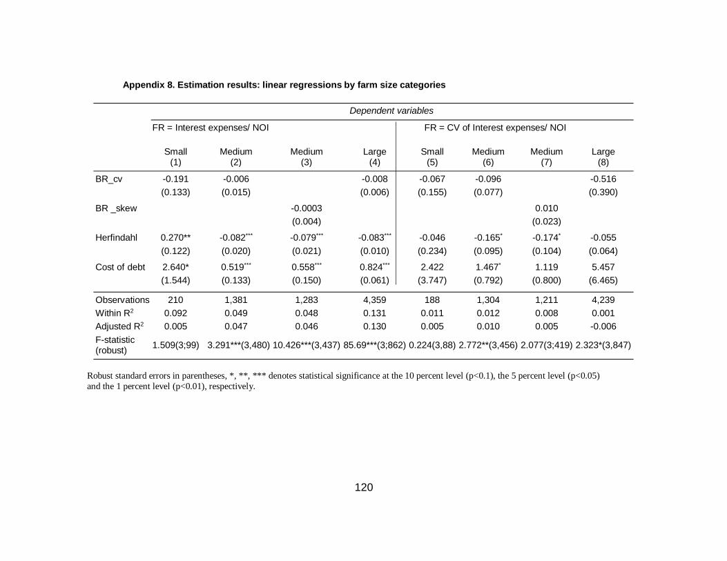
120

Appendix 8. Estimation results: linear regressions by farm size categories

Robust standard errors in parentheses, *, **, *** denotes statistical significance at the 10 percent level (p<0.1), the 5 percent level (p<0.05)

and the 1 percent level (p<0.01), respectively.

Dependent variables

FR = Interest expenses/ NOI FR = CV of Interest expenses/ NOI

Small (1)

Medium

(2)

Medium

(3)

Large

(4)

Small

(5)

Medium

(6)

Medium

(7)

Large

(8)

BR_cv -0.191 -0.006 -0.008 -0.067 -0.096 -0.516 (0.133) (0.015) (0.006) (0.155) (0.077) (0.390)

BR _skew -0.0003 0.010

(0.004) (0.023)

Herfindahl 0.270** -0.082*** -0.079*** -0.083*** -0.046 -0.165* -0.174* -0.055 (0.122) (0.020) (0.021) (0.010) (0.234) (0.095) (0.104) (0.064)

Cost of debt 2.640* 0.519*** 0.558*** 0.824*** 2.422 1.467* 1.119 5.457 (1.544) (0.133) (0.150) (0.061) (3.747) (0.792) (0.800) (6.465)

Observations 210 1,381 1,283 4,359 188 1,304 1,211 4,239

Within R2 0.092 0.049 0.048 0.131 0.011 0.012 0.008 0.001

Adjusted R2 0.005 0.047 0.046 0.130 0.005 0.010 0.005 -0.006


1.509(3;99) 3.291***(3,480) 10.426***(3,437) 85.69***(3;862) 0.224(3,88) 2.772**(3,456) 2.077(3;419) 2.323*(3,847)