Embed Size (px)
Citation preview

Research Collection
Doctoral Thesis
Feasibility study to measure time reversal invariance inpolarized neutron decay
Author(s): Conti, Davide
Publication Date: 1999
Permanent Link: https://doi.org/10.3929/ethz-a-003837499
Rights / License: In Copyright - Non-Commercial Use Permitted
This page was generated automatically upon download from the ETH Zurich Research Collection. For moreinformation please consult the Terms of use.
ETH Library
Diss. ETH No. 13366
Feasibility Study to measure Time Reversal Invariance in
Polarized Neutron Decay
A dissertation submitted to the
SWISS FEDERAL INSTITUTE OF TECHNOLOGY
ZÜRICH
for the degree of
Doctor of Natural Sciences
presented by
Davide Conti
Dipl. Phys. ETH
born on May 19-th, 1968
citizen of Chiasso (TI)
accepted on the recommendation of
Prof. Dr. J. Lang, examiner
Prof. Dr. A. Serebrov, co-examiner
PD Dr. J. Sromicki, co-examiner
Zürich 1999
Contents
Abstract 3
Riassunto 5
1 Introduction 7
2 Theory 9
2.1 General ß - decay 9
2.2 Standard Model Hamiltonian 10
2.3 Physics beyond the standard model 11
2.3.1 Generalized Hamiltonian 11
2.3.2 Neutron decay parameters 11
2.3.3 Time inversion and Triple Correlation experiments 12
3 Experimental Techniques 13
3.1 Experimental Principles 13
3.2 The Beam line at SINQ 20
3.3 Multiple scattering effects 23
3.4 Estimation of the data taking time 25
4 Detector and Experimental Setup 29
4.1 Experimental setup 29
4.1.1 Chamber 32
4.2 Chamber readout electronics 34
4.3 Experimental procedures and optimizations 36
4.3.1 Gas mixture 36
4.3.2 Anode hit multiplicity and time window 39
4.3.3 Cathode hit multiplicity 40
4.4 Chamber setup procedure 42
1
2
4.5 Scintillator calibration 44
5 Data Analysis 47
5.1 Data structure and general concept 47
5.2 Data filters 48
5.3 Fitting routine 49
6 Results 55
6.1 Cosmic ray background 55
6.2 Position Resolution 57
6.3 Angular Resolution 60
6.4 Single Track experiments with the Tl source 63
6.5 Backscattering experiments 66
7 Summary and Conclusions 77
Bibliography 81
List of figures 84
Acknowledgments 87
Curriculum Vitae 89
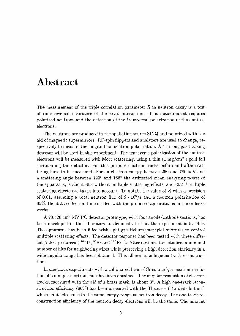
Abstract
The measurement of the triple correlation parameter R in neutron decay is a test
of time reversal invariance of the weak interaction. This measurement requires
polarized neutrons and the detection of the transversal polarization of the emitted
electrons.
The neutrons are produced in the spallation source SINQ and polarized with the
aid of magnetic supermirrors. RF-spin flippers and analyzers are used to change, re¬
spectively to measure the longitudinal neutron polarization. Alm long gas tracking
detector will be used in this experiment. The transverse polarization of the emitted
electrons will be measured with Mott scattering, using a thin (1 mg/cm2 ) gold foil
surrounding the detector. For this purpose electron tracks before and after scat¬
tering have to be measured. For an electron energy between 250 and 780 keV and
a scattering angle between 120° and 160° the estimated mean analyzing power of
the apparatus, is about -0.3 without multiple scattering effects, and -0.2 if multiple
scattering effects are taken into account. To obtain the value of R with a precision
of 0.01, assuming a total neutron flux of 2 • 109/s and a neutron polarization of
95%, the data collection time needed with the proposed apparatus is in the order of
weeks.
A 20x20 cm2 MWPC detector prototype, with four anode/cathode sections, has
been developed in the laboratory to demonstrate that the experiment is feasible.
The apparatus has been filled with light gas Helium/methylal mixtures to control
multiple scattering effects. The detector response has been tested with three differ¬
ent /3-decay sources ( 204T1, 90Sr and 106Ru ). After optimization studies, a minimal
number of hits for neighboring wires while preserving a high detection efficiency in a
wide angular range has been obtained. This allows unambiguous track reconstruc¬
tion.
In one-track experiments with a collimated beam ( Sr-source ), a position resolu¬
tion of 2 mm per electron track has been obtained. The angular resolution of electron
tracks, measured with the aid of a brass mask, is about 3°. A high one-track recon¬
struction efficiency (80%) has been measured with the Tl source ( An distribution )which emits electrons in the same energy range as neutron decay. The one-track re¬
construction efficiency of the neutron decay electrons will be the same. The amount
3
4
of one-track events produced by ambient background ( laboratory measurements )is very low (1:1000).
Backscattering experiments have been done using 17 mg/cm2 thick Pb foils and
different geometrical setups. Wire chambers with different wire diameters have
been used. Tracks of electrons scattered from the polarimeter foil have been recon¬
structed with high efficiency. The scattering vertex has been determined with a pre¬
cision of ~ 7 mm what allows for a clean identification of the two-track backgroundevents produced by electrons scattering on chamber wires. The calculated ratio be¬
tween electrons scattered on wires and electrons scattered on the foil has been found
in agreement with the experimental results. An excellent background/signal ratio
( between 1:100 and 1:1000 depending on the setup ) has been obtained in laboratory
conditions.
The results show that the measurement of the R parameter in neutron decay is
feasible and that the test apparatus developed in this work can be used in the first
studies with the neutron beam.
Riassunto
La misurazione nel decadimento del neutrone del parametro R di tripla correlazione
é un test dell' invarianza della forza debole rispetto all' inversione temporale. Per
lo svolgimento di questo esperimento sono indispensabili neutroni polarizzati come
pure il rilevamento della polarizzazione trasversale degli elettroni emessi.
I neutroni, che sono prodotti dalla sorgente di spallazione SINQ, sono polar¬
izzati con 1' aiuto di superspecchi magnetici. La polarizzazione longitudinale dei
neutroni viene cambiata, rispettivamente misurata, tramite spin-flippers a radiofre-
quenza e analizzatori. Un rivelatore di tracce a gas lungo un metro verra utilizzato
per questo esperimento. La polarizzazione trasversale degli elettroni emessi verra
misurata tramite diffusione Mott, utilizzando un sottile foglio d'oro ( 1 mg/cm2 )che circonderà il rivelatore. Per questo scopo le traiettorie degli elettroni devono
essere misurate prima e dopo la diffusione. II potere d' analisi dell' apparecchio, per
un' energia degli elettroni tra 280 e 780 keV e un angolo di diffusione tra 120° e
160°, é più o meno -0.3 senza tenere in conto effetti di diffusione multipla e -0.2 se
sono tenuti in conto. Assumendo un flusso totale di 2 • 109/s e una polarizzazione
dei neutroni di 95%, il tempo richiesto per ottenere il valore di R con una precisione
di 0.01 é dell'ordine di settimane.
Un prototipo del rivelatore, una camera a fili di 20x20 cm2 composta da quattro
sezioni anodo/catodo, é stato sviluppato nel nostro laboratorio per dimostrare la
fattibilità di questo esperimento. II rivelatore é stato riempito com miscele di gas
leggeri (Elio/methylal) per controllare effetti di diffusione multipla degli elettroni.
La risposta del rivelatore é stata studiata con tre tipi differenti di sorgenti ß ( 204T1,90Sr e 106Ru ). Attraverso studi di ottimizzazione é stato ottenuto che un numéro
minimo di segnali venga emesso da fili adiacenti, pur mantenendo un' efficienza di
rivelazione elevata. Questo permette una ricostruzione inequivocabile delle tracce
delle particelle.
Per ottenere la risoluzione spaziale (2 mm) di una singola traiettoria é stato
utilizzato un fascio collimato di elettroni ( sorgente: Sr ). La risoluzione angolaredelle traiettorie, misurata utilizzando una maschera di ottone, é di circa 3°. Con
l'aiuto della sorgente Tl ( distribuzione An ), che émette elettroni nello stesso spettro
d'energia del decadimento del neutrone, é stata misurata un'elevata efficienza (80%)
5
6
nel ricostruire singole traiettorie. La stessa efficienza é prevista per il decadimento
del neutrone. La quantità di eventi a traccia singola prodotti dal rumore ambientale
( misurazioni di laboratorio ) é molto bassa (1:1000).
Esperimenti di diffusione Mott sono stati fatti utilizzando fogli di piombo (Pb)
spessi 17 mg/cm2 e diverse configurazioni geometriche dell'apparecchiatura. Rivela-
tori con fili di diametro différente sono stati utilizzati. Le traiettorie degli elettroni
diffusi dal foglio di polarimetria sono state ricostruite con un' efficienza elevata. II
vertice di diffusione é stato determinato con una precisione di circa 7 mm, permet-
tendo in questo modo una identificazione chiara di quegli eventi di disturbo che sono
provocati da elettroni diffusi dai fili della camera. II rapporto fra elettroni diffusi
dal foglio ed elettroni diffusi dai fili é stato calcolato ed una buona concordanza con
i risultati sperimentali é stata trovata. Un rapporto eccellente tra rumore e segnale
( fra 1:100 and 1:1000 a seconda della configurazione ) é stato ottenuto in condizioni
di laboratorio.
Questi risultati dimostrano che la misurazione del paramétra R nel decadimento
del neutrone é fattibile e che l'apparecchiatura sviluppata in questa tesi puo essere
utilizzata per i primi studi col fascio di neutroni.
Chapter 1
Introduction
Conservation laws are essential for the formulation of physical theories. In many
cases, the ultimate origin of these laws lies in the space-time properties of the uni¬
verse. For example, from the uniformity and isotropy of space, translation and
rotational invariance follows and this leads inevitably to the linear and angular mo¬
mentum conservation laws. Until 1955 invariance under space inversion ( or parity
transformation ) was also included into the list of space symmetries.
It was in 1956, that, against the common tendency, Lee and Yang [1] published
a hypothesis in which parity conservation in weak decays was called in question.
Soon after, Wu and collaborators [2] discovered substantial parity violation effects
in the /?-decay of Co60.
These unexpected results forced the physics community to examine the validity
of the invariance laws for all the discrete symmetries. The outcome of this still
not finished investigation has been the V-A theory of the weak interaction and the
discovery of the violation of the CP symmetry in the K-decay system [3], While
the first result lead to the observation of the gauge bosons W±, Z [4, 5] and to
the spectacular unification of electromagnetic and weak theories [6], the ultimate
origin of the CP-violation has not yet been clarified. Moreover, due to the strong
experimental and theoretical arguments which assess the invariance of the physical
laws under the CPT transformation [7], CP violation is directly linked with violation
of time reversal symmetry T.
Other indications of T-symmetry breaking appear from cosmological observa¬
tions: in particular the enormous surplus of cosmic matter over antimatter is taken
as an evidence for a time reversal violating (TRV) interaction of different nature
than the one present in K-decay [8].
In order to understand the nature of the CP violation a TRV signal in other
systems would be very useful, therefore many nuclear physics projects searching for
a T violation have been carried out.
For example time reversal has been tested in the strong interaction by performing
7
8 CHAPTER 1: INTRODUCTION
detailed balance measurements [9] in the system 27Al+p ¥" 24Mg + a. Very precise
TRV experiments have been the search for an electric dipole moment (EDM) of the
neutron [10] or of atomic systems [11].In nuclear /?-decay the CP violating effects observed in the K-system are too
weak to be observed [12], therefore any TRV sign in these processes would indicate
the presence of a new physical process.
Beta decay experiments, suggested for the first time by Jackson [13], are per¬
formed by looking at the triple product of three decay observables. Following Jack¬
son, these TRV investigations are referred as "D" and "R" parameter measurements.
Both experiments require the production of polarized nuclei and the detection of the
ß particle momenta. In the case of D the third observable is given by the momentum
of the recoil nucleus, whereas for R it is given by the polarization of the emitted
electron. However the physical processes detectable by these two quantities are
completely different: a nonzero value of D, which is sensitive to the imaginary part
of the vector and axial vector coupling constants, could be generated by a mas¬
sive right-handed weak boson [12] while non-vanishing values of R, proportional to
the imaginary part of the scalar and tensor coupling constants, would indicate an
exchange of a charged Higgs boson or leptoquarks [14].While the D parameter has been already the subject of a lot of investigations
[15, 16, 17, 18], for a long time R has not been measured with comparable precision
[19]. Only recently the measurement of R in the 8Li decay [20] has provided very
stringent limits for the imaginary part of the tensor coupling constants *. In the
scalar sector this quantity is still one order of magnitude less precise [19], therefore
a similar improvement there would be very valuable.
Neutron decay is a very good candidate for such a study, since the mixing of Fermi
and Gamow-Teller transitions is necessary for a sensitivity to the scalar components
of the time reversal violating interaction. The neutron matrix elements are precisely
known and the contribution to R from the electromagnetic forces ( the final state
interaction ) is small. In addition, the last missing coefficient would be added to
the set of measured neutron decay parameters, what is of great value for theoretical
calculations. From the experimental point of view neutrons are highly polarizable
and the analyzing power for Mott scattering of the emitted electrons is large.
This is the motivation behind our attempt to measure for the first time the R
correlation in the neutron decay. The purpose of this dissertation is to study the
feasibility of this experiment and trace the way for an effective realization of the
project.
1 Scalar quantities are involved when Fermi types of /3-decay are present in the nuclear Hamil-
tonian. The 8Li decay is dominated by a Gamow-Teller transition, therefore it is particularlysensitive to the tensor coupling constants.
Chapter 2
Theory
2.1 General ß - decay
Beta decay is one of the spontaneous processes by which radioactive nuclei can
reach stability. In this transition a nucléon inside the nucleus changes its isospin
z-component and a lepton pair (e,ue) is created. The charged lepton can be a
positron (/?+) or an electron (ß~), depending on the type of nucleus involved in the
interaction.
A main feature of /3-decay is the broad distribution of the charged lepton energy,
which in 1930 lead Pauli to the famous neutrino hypothesis. The total energy release
in this transition is usually smaller than few MeV. In this energy range the lengthof the lepton wave is larger than the nuclear size and the e, ue wavefunctions can be
approximated, for many purposes, as plane waves. In the /3-decay theory, the plane
waves are expanded according to the orbital angular momentum Lh carried away
by the leptons. This allows to classify /3-decays into allowed (L = 0) or forbidden
(L =£ 0) transitions. The degree of forbiddenness depends on the lowest nonzero
value of orbital angular momentum Lh entering in the lepton wave expansions. In
allowed decays, the highest value of the lepton wave functions is inside the nucleus,
therefore the probability of a transition is maximal in this case. These are the fastest
decays.
Transitions with L = 0 and the spins of the emitted leptons antiparallel are
referred as Fermi interactions. In this case the z-component of the nuclear angular
momentum is conserved. Otherwise, if the spins of the leptons are parallel the
transitions are classified as Gamow-Teller type. The parity of the nucleus cannot be
changed by allowed transitions.
Parity changes between mother and daughter nucleus, are possible only in case
of forbidden decays. These are highly suppressed transitions because the lepton
wavefunctions must vanish at the nuclear center. As a rule, to every degree n of
forbiddenness corresponds an orders of magnitude increase in the lifetime.
9
10 CHAPTER 2: THEORY
2.2 Standard Model Hamiltonian
In the framework of the Standard Model /3~-decay is represented by the exchange of
a weak charged boson W between quarks and leptons in the limit of low momentum
transfer. The properties of W determine the interaction to be a vector - axial vector
type, and to couple only with left-handed fermions [12].On the level of quarks the respective Hamiltonian [21] for a transition
d —y e~~ + u + z7e is assumed as:
H = ^Vudelß(l - 75H • «7"(1 - 75)d + h.c. (2.1)
where Gp is the Fermi coupling constant, VU(j is an element in the Cabibbo
Kobayashi Maskawa (CKM) matrix, jß are the Dirac 7-matrices* and h.c. is the
hermitian conjugate term, so that (2.1) is a real defined quantity. The analogous of
eq. (2.1) for nuclei, takes into account the interaction of nucléons inside the nucleus.
In case of free neutron decay :
n -)> e~ +p + z7e (2.2)
the Hamiltonian becomes:
H = g- Welß{l ~ 7s)VVe WpYiCv - CAj5)il>n (2.3)
where g = %Kd, and MF = ipp^ßtjjn, MGt = fpp^Jsipn, are identified as the
Fermi respectively the Gamow-Teller transition matrix elements.
The two coupling constants Ca and Cy usually called the vector and axial vector
formfactors take into account the binding of the quarks in the nucléon. Their exper¬
imental values, Cy=\ and Ca=-1-25, are close to 1. Theoretically the value of Cv
can be explained by the fact that the cloud of virtual pions surrounding the neutron
does not change the magnitude of the weak interaction, the so called conserved vec¬
tor current (CVC) hypothesis. With similar but more complicated arguments, the
partially conserved axial vector current (PCAC) assumption, can be used to show
[22] that Ca should also not be very far from unity.
1Through this work ( see also the discussion in [21] ) the convention of Jackson [13] 75 =
7x727374 and 74 = 70 with Cv = C'v = 1 and CA = C'A = -1.25 is used.
2.3. PHYSICS BEYOND THE STANDARD MODEL 11
2.3 Physics beyond the standard model
2.3.1 Generalized Hamiltonian
Vector and axial vector are not the only possible forms of weak interaction.
In general, Lorentz invariance allows five possible forms, the scalar (S), vector
(V), tensor (T), axial vector (A) or pseudoscalar (P) interaction.
The resulting Hamiltonian [1] is:
H = g- £ (TACi ~ C'n5]^e) (fpIi;n) + h.c. (2.4)I=S,V,T,A,P
where the operators I are the S,V,T,A,P combinations 1,7^,7757^71/, •••of the
Dirac-7 matrices and g represents the strength of the weak interaction.
The coefficients C are related to the helicity of the fermions. In case of absence
of right handed neutrinos Cx = C\ has to be inserted.
2.3.2 Neutron decay parameters
Correlations between the different particles (e, ue,p, n) involved in neutron decay are
described by the neutron decay parameters. To obtain these quantities, observables
like the neutron polarization J, the electron momentum p"e, the neutrino momentum
pZe or the electron spin ae have to be measured. The dependence of the decay
probability from these quantities is:
W oc (1 +4^ + AJ-ß ++B^ + Df- tfx^
+ RLM^1 + ,.,)
(2.5)In neutron decay, the strength of the weak interaction g can be calculated from
lifetime (r„) measurements [7]:
rn = 887.0 ± 25 (2.6)
For this decay, the Fermi and Gamow-Teller matrix elements |Mf|2 = 1 ;
|-^gt|2 = 3 present no theoretical uncertainties. Therefore it is easy to relate
experimental values of the neutron parameters to theoretical predictions.
For example, the asymmetry parameter A has been recently a subject of several
investigations [23, 24, 25] because of a discrepancy between the S.M. predicted value
and the measured ones. The latest result [25]:
A =-0.1189(12) (2.7)
is again in agreement with the S.M. predictions.
12 CHAPTER 2: THEORY
Jackson [13] linked the coupling constants Ci,C'j with the decay parameters.
The relationships for the R and D parameters are:
DC = MGTMF]jj^j-2Im(CsC^-CvC*A + C'sC^-CvC'*)
RÇ = \MGT\2-i—-2Im{CTC'2 + arCA) +
+MgtMfJj^-j 2Im(CsC'X + C'SCA + CVC% + C'VC*T)
i = |MF|2(|Cs|2 + |Cy|2+|C^|2 + |C(,|2)
+ |MGT|2(|Cr|2 + \CA\2 + \C'T\2 + \C'A\2) (2.8)
Inserting the values of Mqt and Mp and using equations (2.8) for the neutron
decay, one can observe ( assuming CT small ) that R is primarily dependent on the
magnitude of the imaginary scalar and tensor couplings, while D provides in the
first order access to the complex values of Ca and Cy.
2.3.3 Time inversion and Triple Correlation experiments
To study TRV effects in ß decay it is necessary to measure at least three vector or
axial-vector quantities. The D and R parameters transform the following way under
the P and T symmetry:
p T -
D : J -(feXpZj -> D: J (-pe x -pZe) -> -D :-J (~pe x -j£e)
R: J (ae x pe) -> -R-.-J- {~ae x -pe) -)• -R : -J • (-ae x -pe)(2.9)
While the D-parameter is P even and T odd, the R-parameter is P odd and
T odd, therefore only a parity violating interaction can provide a TRV signal in a
R measurement.
However in an experiment for which the time arrow is really reversed, not only
the spins and momenta have to be changed, but also the order between decaying
particles and decay products has to be inverted [26]. Because of this, correction
terms have to be added to the expressions (2.8) for R and D. In the case of R we
have [27]:
Rc.{: = -Z-^-A (2.10)Pe
The attractive feature of the neutron decay is that these corrections, caused mainly
by the Coulomb force, are small.
Chapter 3
Experimental Techniques
3.1 Experimental Principles
Measurements of the R parameter require polarized nuclei or particles and detec¬
tion of the transversal polarization of emitted electrons. While highly polarized
neutron beams are available in many research facilities, the second quantity has to
be extracted with the aid of an efficient detection Polarimeter.
Mott scattering of electrons from heavy nuclei is an interesting polarimetry tech¬
nique. This technique is based on the spin-orbit coupling of electrons in the field
of nuclei. With electrons polarized transversally to the scattering plane this effect
causes a left-right asymmetry of scattered electrons. Although the cross section is
reduced for large scattering angles, this method is attractive since the analyzing
power S(fi) of Mott scattering for electrons in the few 100 keV energy range is quite
high ( between 0.1 and 0.4 ) for large scattering angles ( ê ~ 140° ).
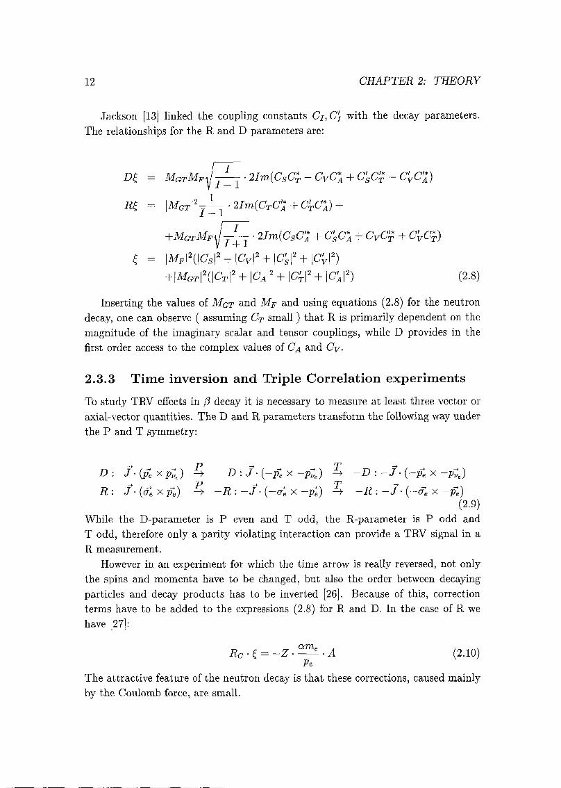
The principle of our experiment, shown in figure 3.1, is based on this polarimetry
technique:
For simplicity we take into account only decay electrons emitted with a momentum—*
pe perpendicular to the neutron polarization J. In this case, for a nonzero value
of the R parameter, according to equation (2.5), a transversal electron polarization
aT2 ~ R . J perpendicular to the neutron polarization is induced. Consider now
electrons scattered back under the scattering angle $s by the Mott Polarimeter (a thin gold foil ). The asymmetry of scattered electrons between the two states of
the neutron polarization ±J is proportional to R J S(us)- The value of R can be
calculated from the measured asymmetry and neutron polarization and the known
analyzing power S(es).To determine the emission and scattering angle of the electrons, a tracking de¬
tector is used. Such a device could consist of a set of MWPC's surrounded by the
Polarimeter foil. Finally, scintillators measure the energy of the particles and trigger
the detector.
13
14 CHAPTER 3: EXPERIMENTAL TECHNIQUES
J
Figure 3.1: Principle of the experiment. We measure the asymmetry of scattered
electrons ( emission momentum: pe, scattering momentum: p~s ) for two states ±J
of the neutron polarization. In case of R^ 0, a transversal electron polarization aT2
orthogonal to J is induced. Because gt2 —> —&t2 IS reversed by flipping the neutron
polarization, the value of R can be extracted from the measured asymmetry.
decay irack
trackingdetector
neutron decay channel
Gold Foil
\y
Gold Foil
ii.rn'injiirrfjfniitrtirtfii.iii'rjtjirrinrrt^r-i
Scintillators
decoy tracktracking
detector
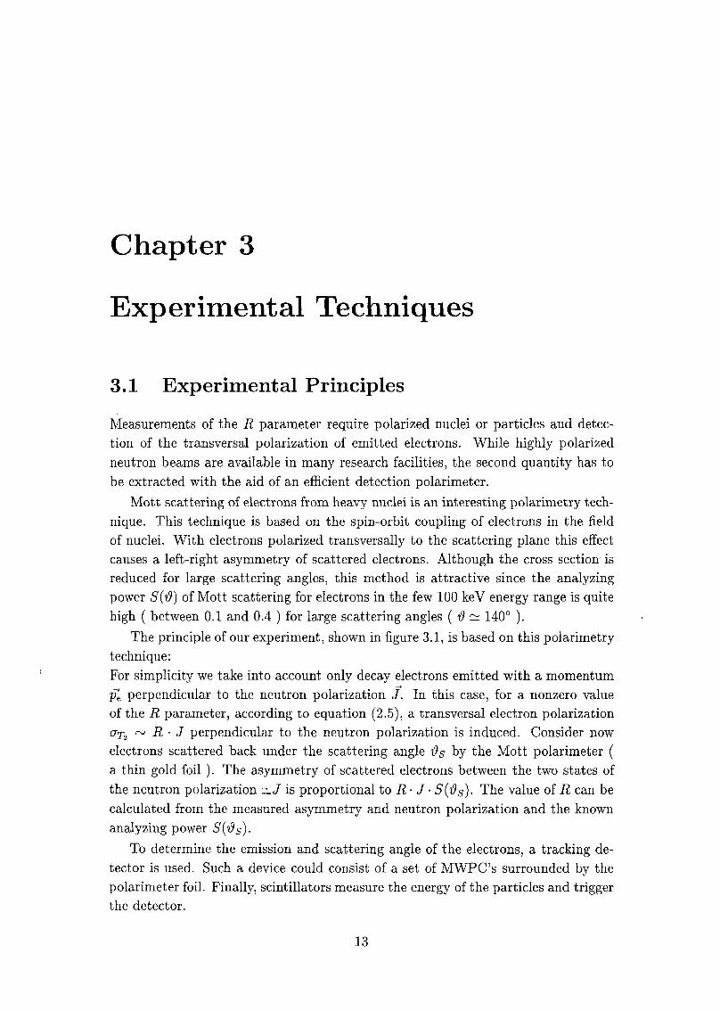
Figure 3.2: Schematic view of the cylindrical experimental setup used in calculations.
To maximize the counting statistics, a longitudinal beam polarization and an
experimental apparatus with cylindrical shape, like the one of figure 3.2, are most
suitable. This arrangement may have also some advantages in reduction of sys¬
tematic effects. In addition, calculations for a cylindrical detector are particularly
simple, therefore in this section such a configuration will be discussed.
3.1. EXPERIMENTAL PRINCIPLES 15
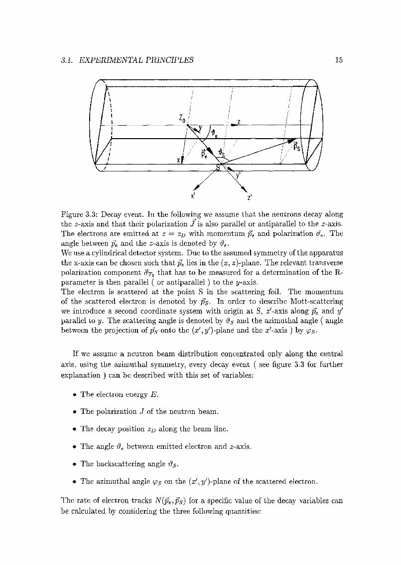
Figure 3.3: Decay event. In the following we assume that the neutrons decay alongthe z-axis and that their polarization J is also parallel or antiparallel to the z-axis.
The electrons are emitted at z — zD with momentum pe and polarization ae. The
angle between pe and the z-axis is denoted by #e.
We use a cylindrical detector system. Due to the assumed symmetry of the apparatus
the x-axis can be chosen such that pe lies in the (x, z)-plane. The relevant transverse
polarization component <tt2 that has to be measured for a determination of the R-
parameter is then parallel ( or antiparallel ) to the y-axis.
The electron is scattered at the point S in the scattering foil. The momentum
of the scattered electron is denoted by ps. In order to describe Mott-scatteringwe introduce a second coordinate system with origin at S, z'-axis along pe and y'
parallel to y. The scattering angle is denoted by $5 and the azimuthal angle ( anglebetween the projection of ps onto the (x',y')-plane and the x'-axis ) by ips-
If we assume a neutron beam distribution concentrated only along the central
axis, using the azimuthal symmetry, every decay event ( see figure 3.3 for further
explanation ) can be described with this set of variables:
• The electron energy E.
• The polarization J of the neutron beam.
• The decay position zr> along the beam line.
• The angle êe between emitted electron and z-axis.
• The backscattering angle 'as-
• The azimuthal angle <ps on the (x', y')-plane of the scattered electron.
The rate of electron tracks N(pe,ps) for a specific value of the decay variables can
be calculated by considering the three following quantities:
16 CHAPTER 3: EXPERIMENTAL TECHNIQUES
• The decay rate N± of neutrons having a neutron polarization ±J parallel (+)or antiparallel (-) to z.
• The emission probability We(pe) of electrons having the spin parallel (©) or
antiparallel (®) to the y-axis by known neutron polarization ±J and electron
momentum pe.
• The backscattering probability Ws(pe,ps) of electrons, by known electron spin
state (0,<8>), electron momentum pe and backscattered electron momentum ps-
The total neutron decay rate N [s_1] is calculated in section 3.4.In the following
we assume that the magnitude of the neutron polarization J as well as the magnitude
of the neutron flux N are not changed by flipping the neutron spin polarization.
Since the neutron polarization is flipped at constant time intervals, only half of the
rate is available per polarization state and we have N+ = iV_ = N/2.To calculate the electron emission probability We(pe) we have first to consider
the emission energy spectrum W(E) for unpolarized electrons. Since neutron decay
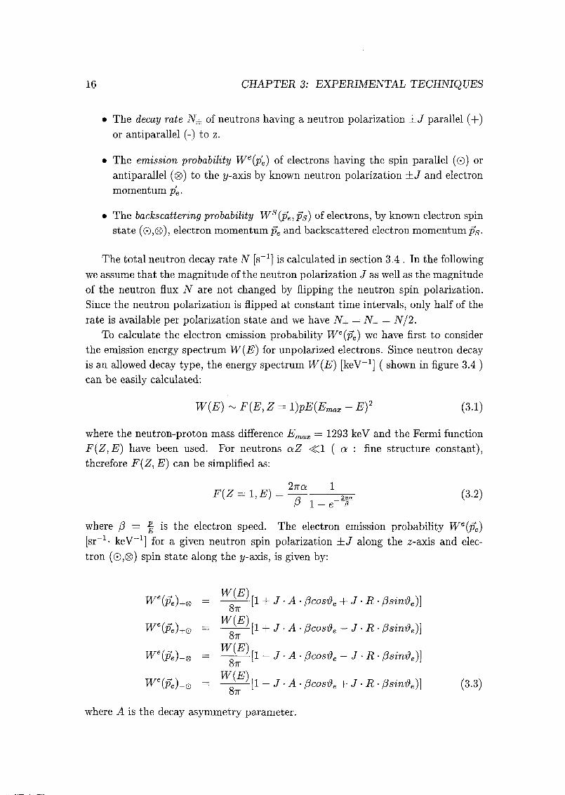
is an allowed decay type, the energy spectrum W(E) [keV-1] ( shown in figure 3.4 )can be easily calculated:
W(E) ~ F{E, Z = l)PE(Emax - Ef (3.1)
where the neutron-proton mass difference Emax = 1293 keV and the Fermi function
F(Z,E) have been used. For neutrons aZ <Cl ( a : fine structure constant),therefore F(Z, E) can be simplified as:
F(Z = 1,E) = 2^ ^__(3.2)
P 1 -e ß
where ß = ^ is the electron speed. The electron emission probability We(pe)[sr_1- keV-1] for a given neutron spin polarization ±J along the z-axis and elec¬
tron (0,®) spin state along the y-axis, is given by:
We(pe)+® = ^f^[l + J-A-ßcosee + J-R-ßsin$e)}on
We(pe)+Q = y^p-[l + J A ßcos0e - J R ßsin0e)]
We(pe)_® = —^-[l-J-A-ßcosVe-J-R-ßsinde)}Ö7T
We(pe)_Q = —^[1- J-A-ßcosee + J-R-ßsin$e)} (3.3)on
where A is the decay asymmetry parameter.
3.1. EXPERIMENTAL PRINCIPLES 17
x10"
400 600 800
Kinetic Energy [keV]
Figure 3.4: The energy spectrum W(E) of decay electrons calculated with (3.1).
3>
Tn
o
-0.1
-0.2
-0.3
-0.4
-0.5
-0.6100 120 140
100 keV
200 keV
300 keV
400 keV
500 keV
600 keV
700 keV
-
'-*
;;
=~
""*.,-
,.Z- .--"_ -
"
I 1
••u»il*E;(;-•»»»z„^inii~
'
1
100 keV
200 keV
300 keV
400 keV500 keV
600 keV
700 keV
160
1>
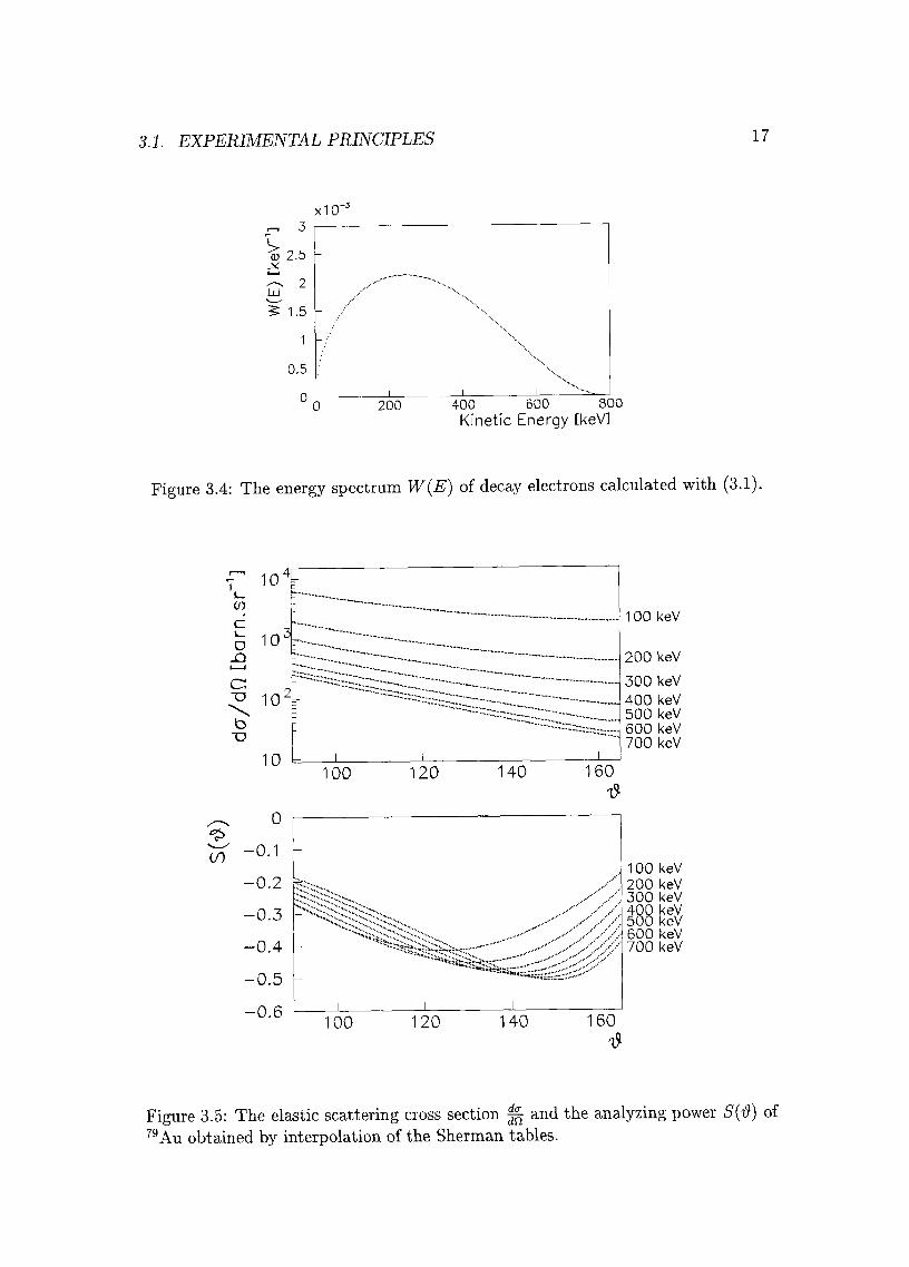
Figure 3.5: The elastic scattering cross section ^ and the analyzing power 5(i9) of
79Au obtained by interpolation of the Sherman tables.
18 CHAPTER 3: EXPERIMENTAL TECHNIQUES
To calculate the electron backscattering probability Ws(pe,ps), the differential
elastic cross section Jp and the Mott scattering analyzing power 5(#s) for gold
have to be known. For numerical calculations, we use interpolated values of ^and 5($) given in the Sherman tables [28] for 80Hg. Figure 3.5 shows the angular
dependence of these two functions at various energies. For electrons with spin state
parallel or antiparallel to the y-axis (0, ©) Ws [sr~2- keV-1] is :
rS{-, ^_
,mda l + S($s)cosipsWb(pe,ps)®~T
dds sindp
where T is the gold foil thickness [mg/cm2] and the term siwdg takes into account
the increase of T for inclined emission angles.
After having calculated the three terms N±, We(pe) and Ws(pe,ps), we combine
them to find the intensity of electron scatterings N(pe,ps) by given beam polariza¬
tion (±) and transversal electron spin orientation (0,®). This gives four terms,
N+®(pe,ps), N+G(pe,ps), N-®(pe,ps) and N^Q(pe,ps) .For example N+®(pe,ps)
[sr-2- keV_1-s-1] is given by:
N+®(peJs) = N+-We(pe)+®-Ws(pe,ps)®~N W(E) da
.
l + S(ês)cos<ps~
T.Y.-cr-— -[l + J.A.ßcos*e + J.R.ß8tn*e)] —j-e
(3.5)
In the experiment however, we don't know the transversal spin orientation (©, ®)of the decay electrons and we are interested only in N±(pe,ps) [sr-2- keV^-s-1]which is the number of electron scatterings with momenta pe and ps by given beam
polarization. Therefore we sum over the electron spin states:
N±{pe,Ps) = N±®(pe,ps) + N±G(pe,ps) (3.6)
Explicitly:
N W(E) da l±J-A-ßcostie±J-R-ßsintfecos<psS('ds)N±(pe,Ps) ~T
2 47T dfls siwde
(3.7)
The total asymmetry can be obtained by integrating N±(pe,ps) over the detector.
We define "left" (L) scatterings for electrons with -90° < cps < 90° and "right" (R)
scatterings for electrons with 90° < ps < 270°.

3.1. EXPERIMENTAL PRINCIPLES 19
The numbers of scatterings N+L, N_L, N+R, iV_B, [s x] are defined as:
rn/2
d(fs / dzDdEdiïesiri'dsd'ôsN+(pe,ps)-TT/2 J
/•3tt/2 p
N+r = / ^5 / dzDdEduesinêsddsN+(pe,ps)J-k/2 J
j-k/2 çiV_i = / d<ps / dzDdEdQesin'dsd'dsN-('pe,ps)
J-k/2 J
fin/2 r
iV_B = / dtps / dzDdEdUesinêsd'ôsN^(pe,ps) (3.8)./ir/2 j
where the limits of the integrals on E,z,tte and Us depend from the energy cutoff
and the detector geometry.
We introduce now the quantities < a >, < A > and < S >:
*/2j f J JEun a jq
^(^) dcT/
d<£>5 /
dzudEdtleSind
J—k/2 J
< a > =/
d^c / dzndEdÇleSin'dsd'dsavs-
<A> =
r/2/
Ansiw&e dCts
1 /"7I72 /" W(£?) der• / dw5 / dzDdEdVLesindsdds—: ——ßctgee
a>
J-k/2 JAn
dus
<a>
J-k/2
JAn
ails
1 f*l2 r W(E) da
/ dips / dzDdEdQesin'dsd'ds—. —/< a > J—k/2 J An dils
(3.9)
With these definitions we can express now N+l,N+r,N^l,N_r as1
N
N+L~ —T <a> -[1 + JA- < A > +JR- <S>]Lt
NN+r ~ —T < a > -[1 + JA- < A > -JR- <S>]
Li
NN_L T < a > -[1 - JA- < A > -JR- < S >]
Li
NN_R ~—T<a>-[l-JA-<A> +JR- < S >} (3.10)
Li
If we introduce now the double ratio r :
V N.LN+R
Then an asymmetry e from r can be built as:
r-1e =
r + 1
(3.11)
(3.12)
1Note that ( for a symmetric detector ) changing the integration range of <ps in (3.9) from "left"
to "right" values leaves < a > and < A > unchanged whereas < S > becomes — < S >.
20 CHAPTER 3: EXPERIMENTAL TECHNIQUES
This asymmetry is particularly insensitive to systematic effects [29] and, in the
case of a symmetric left-right detector geometry and a perfect alignment of the
polarization, we can express it as:
e =1
1at>Rau^<S>RJ (3.13)
1- (AJ < A >)2
where the small value of the decay asymmetry A ~ 0.1 has been used in the last
approximation. Therefore by measuring e the value of R can be extracted.
3.2 The Beam line at SINQ
Because of the high available intensity and the low speed of neutrons which leads
to a high decay rate, a beam of cold neutrons is best suited for this experiment.At PSI cold neutrons are produced at the recently constructed spallation source
SINQ. The primary 600 MeV proton beam from the ring accelerator is directed ver¬
tically upwards to the bottom of the SINQ spallation target, an alloy of zirconium
and lead ( Zircalloy ) possessing high mechanical strength and high melting tem¬
perature. The beam, with an intensity of about 1 mA, hitting the target material
releases around 3 • 1016/s neutrons [30] with kinetic energies of a few tens of MeV.
A 2 m diameter D2O moderator tank surrounding the target, slows them down in
the thermal range ( mean velocity ~ 2 km/s ). A liquid D2 vessel installed inside
the moderator and connected to the guides, slows them down further into the cold
range. Evacuated tubes inside the tank extract the neutrons from the moderator.
When neutrons achieve thermal energy the scattering form factor approaches a
constant isotropic value, the scattering length b, and their de Broglie wavelength A
becomes comparable with interatomic distances. Therefore neutron scattering from
homogeneous matter becomes a coherent process and can be described as an optical
phenomenon. In this case, neutrons transported in the vacuum tubes can undergototal reflection from the walls, if their glancing angle is below a critical value 9C:
8C = A y/p/Tr (3.14)
with the scattering length density p [m~2] defined as:
P = Pnb (3.15)
where pn [m-3] is the nuclear density, and b [m] is the scattering length.Such neutron guides and neutron mirrors are made usually of evacuated tubes
surrounded with glass walls coated with Ni. But even for 58Ni, the best available
scattering material, the maximal glancing angle for A = 10 Â is still lower than a
degree.
3.2. THE BEAM LINE AT SINQ 21
r-10
CO
1
Eo
8
<
E
6
4
°<
X2
00 2 4 6 8 10
Wavelength A [A]
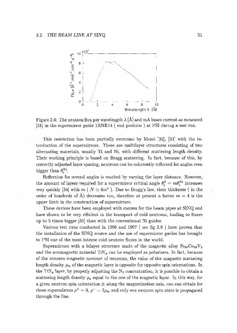
Figure 3.6: The neutron flux per wavelength A [Â] and mA beam current as measured
[31] in the supermirror guide 1RNR14 ( end position ) at PSI during a test run.
This restriction has been partially overcome by Mezei [32], [33] with the in¬
troduction of the supermirrors. These are multilayer structures consisting of two
alternating materials, usually Ti and Ni, with different scattering length density.
Their working principle is based on Bragg scattering. In fact, because of this, by
correctly adjusted layer spacing, neutrons can be coherently reflected for angles even
bigger than 6^\Reflection for several angles is reached by varying the layer distance. However,
the amount of layers required for a supermirror critical angle 9f = md^1 increases
very quickly [34] with m ( N ~ 4m4 ). Due to Bragg's law, their thickness ( in the
order of hundreds of À) decreases too, therefore at present a factor m = A is the
upper limit in the construction of supermirrors.
These devices have been employed with success for the beam pipes at SINQ and
have shown to be very efficient in the transport of cold neutrons, leading to fluxes
up to 5 times bigger [35] than with the conventional Ni guides.
Various test runs conducted in 1996 and 1997 ( see fig 3.6 ) have proven that
the installation of the SINQ source and the use of supermirror guides has brought
to PSI one of the most intense cold neutron fluxes in the world.
Supermirrors with a bilayer structure made of the magnetic alloy Fe50Co48V2
and the nonmagnetic material TiNx can be employed as polarizers. In fact, because
of the nonzero magnetic moment of neutrons, the value of the magnetic scattering
length density pm of the magnetic layer is opposite for opposite spin orientations. In
the TiNa, layer, by properly adjusting the N2 concentration, it is possible to obtain a
scattering length density pn equal to the one of the magnetic layer. In this way, for
a given neutron spin orientation ± along the magnetization axis, one can obtain for
these supermirrors p+ ~ 0, p~ = 2pm and only one neutron spin state is propagated
through the line.
22 CHAPTER 3: EXPERIMENTAL TECHNIQUES
CH
oo
<Dl
^+
col
(Nl
<D
c3<DX)
<D
+->
o
Scd
PU
en
<u
3.3. MULTIPLE SCATTERING EFFECTS 23
Our experiment will be installed on the fundamental physics facility at PSI-
SINQ. This facility has been planned by the spokesman of this experiment, PD Dr.
J.Sromicki, in a tight collaboration with Dr P. Boni ( PSI ), Prof. A.Serebrov and
Dr. A. Schebetov ( PNPI St, Petersburg-Gatchina ).
Thanks to the active engagement of the PSI and PNPI technical teams and
continuous support of PSI management, the facility is in advanced phase of con¬
struction. Because of the short distance between target and experiment ( ~ 15
m ) as well as the final beam size ( 15 x 4 cm2 ) the beam line for fundamental
physics at the SINQ is expected [36] to have a very high polarized cold neutron flux
of ~ 108- s-1- cm'2- mA"1.
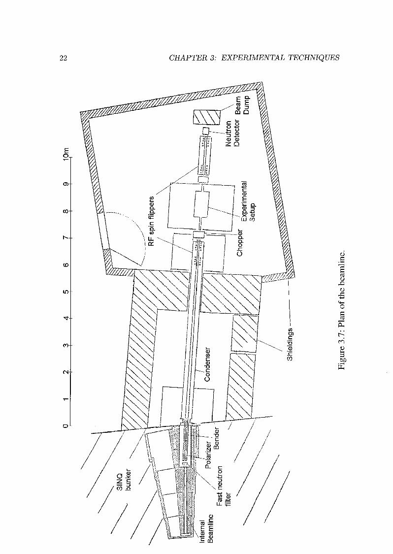
Figure 3.7 shows the general layout of the beamline. The cold neutron guide
starts from the moderator with a straight, high ( m—3 ) reflectivity, supermirror sec¬
tion. Just after, the neutrons will be polarized by a magnetic multislit supermirror
structure. Successively, to remove the background connected with the target as well
as the one coming from the polarizer itself, they will go through a bending section
( bending angle around 2° ). A following long condenser will focus and transport
the neutron beam to the experimental hall where a setup similar to the one of
ref. [37], consisting of two spin flipper devices ( the second one is the polarization
analyzer ), will allow to measure precisely the beam polarization, which is expected
to be around 95%. The experiment will be inserted between the first spin flipper
device and the polarization analyzer.
3.3 Multiple scattering effects
As we have seen, ( section 3.1 ) Mott scattering can be used to detect the transversal
polarization of electrons. The theoretical analyzing power S(9) of this process for a
point nucleus is exactly predicted from analytic solutions [38] of the Dirac equation.
This approximation works well for an electron energy ranging between 100 keV and
1 MeV where nuclear size effects are negligible.
In the experimental case however, the effective value of the analyzing power Seffin a thick target is reduced by multiple scattering effects. To determine the optimal
thickness of the Polarimeter foil for our experiment, the influence of this process,
referred as depolarization, has to be known. Fortunately, for a kinetic energy up
to 700 keV depolarization effects in the elastic scattering of electrons from thin Au
foils have been investigated ( see for ex. [39] ). Above this limit [40] less data is
available, but, for increasing energy, depolarization effects are smaller too.
In our experiment the value of 5 ( see fig 3.5 ) at the scattering angle
9S = 120° is usually close to the maximum. At this angle, for a kinetic energy range
24 CHAPTER 3: EXPERIMENTAL TECHNIQUES
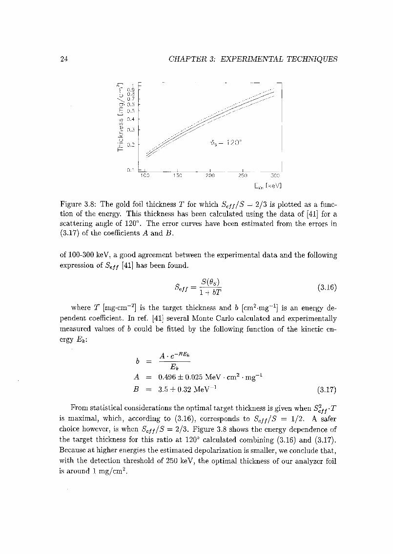
Figure 3.8: The gold foil thickness T for which Seff/S = 2/3 is plotted as a func¬
tion of the energy. This thickness has been calculated using the data of [41] for a
scattering angle of 120°. The error curves have been estimated from the errors in
(3.17) of the coefficients A and B.
of 100-300 keV, a good agreement between the experimental data and the following
expression of Seff [41] has been found.
Seff ~S(9S)1 + bT
(3.16)
where T [mg-cm-2] is the target thickness and b [cm2-mg-1] is an energy de¬
pendent coefficient. In ref. [41] several Monte Carlo calculated and experimentally
measured values of b could be fitted by the following function of the kinetic en¬
ergy Ek:
A e~BEk
A
B
Ek
0.496 ± 0.025 MeV • cm2 • mg"1= 3.5 ± 0.32 MeV
-l
(3.17)
From statistical considerations the optimal target thickness is given when S^^-Tis maximal, which, according to (3.16), corresponds to Seff/S = 1/2. A safer
choice however, is when Seff/S — 2/3. Figure 3.8 shows the energy dependence of
the target thickness for this ratio at 120° calculated combining (3.16) and (3.17).Because at higher energies the estimated depolarization is smaller, we conclude that,
with the detection threshold of 250 keV, the optimal thickness of our analyzer foil
is around 1 mg/cm2.
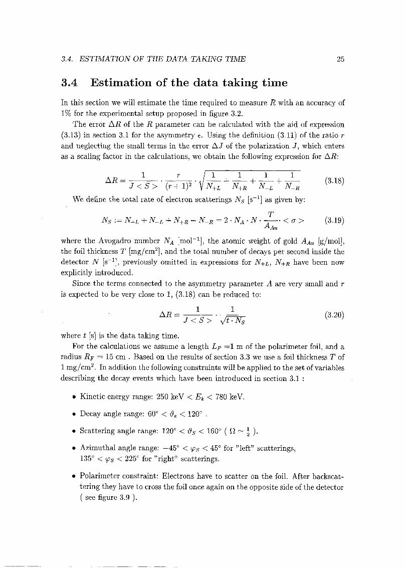
3.4. ESTIMATION OF THE DATA TAKING TIME 25
3.4 Estimation of the data taking time
In this section we will estimate the time required to measure R with an accuracy of
1% for the experimental setup proposed in figure 3.2.
The error AR of the R parameter can be calculated with the aid of expression
(3.13) in section 3.1 for the asymmetry e. Using the definition (3.11) of the ratio r
and neglecting the small terms in the error AJ of the polarization J, which enters
as a scaling factor in the calculations, we obtain the following expression for A.R:
AR=jis^-Jr^-^L + N^R+jtL + ltR (318)
We define the total rate of electron scatterings Ns [s_1] as given by:
Ns := N+L + AU + N+r + N.r = 2-Na-N-~ <a> (3.19)
where the Avogadro number Na [mol-1], the atomic weight of gold Aau [g/mol],the foil thickness T [mg/cm2], and the total number of decays per second inside the
detector N [s_1], previously omitted in expressions for N±l, N±R have been now
explicitly introduced.
Since the terms connected to the asymmetry parameter A are very small and r
is expected to be very close to 1, (3.18) can be reduced to:
&R = ^rA Arr(3-20)
J <S> y^Vsv ;
where t [s] is the data taking time.
For the calculations we assume a length LF =1 m of the Polarimeter foil, and a
radius RF = 15 cm . Based on the results of section 3.3 we use a foil thickness T of
1 mg/cm2. In addition the following constraints will be applied to the set of variables
describing the decay events which have been introduced in section 3.1 :
• Kinetic energy range: 250 keV < Ek < 780 keV.
• Decay angle range: 60° < i9e < 120°.
• Scattering angle range: 120° < -&s < 160° ( O ~ \ ).
• Azimuthal angle range: —45° < ips < 45° for "left" scatterings,135° < <ps < 225° for "right" scatterings.
• Polarimeter constraint: Electrons have to scatter on the foil. After backscat-
tering they have to cross the foil once again on the opposite side of the detector
( see figure 3.9 ).
26 CHAPTER 3: EXPERIMENTAL TECHNIQUES
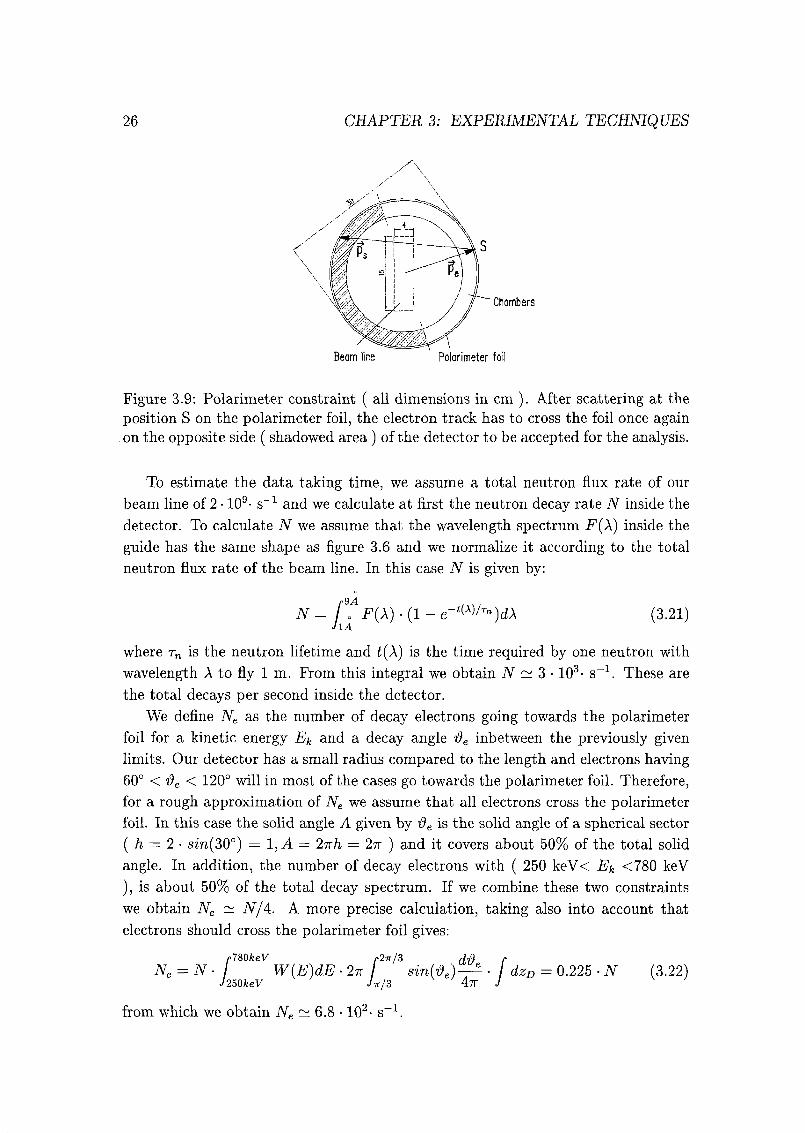
/-,.
'
Chambers
Beam line Polarimeter foil
Figure 3.9: Polarimeter constraint ( all dimensions in cm ). After scattering at the
position S on the Polarimeter foil, the electron track has to cross the foil once againon the opposite side ( shadowed area ) of the detector to be accepted for the analysis.
To estimate the data taking time, we assume a total neutron flux rate of our
beam line of 2 • 109- s'1 and we calculate at first the neutron decay rate N inside the
detector. To calculate N we assume that the wavelength spectrum F(X) inside the
guide has the same shape as figure 3.6 and we normalize it according to the total
neutron flux rate of the beam line. In this case N is given by:
r9A , N,
AT = /„ F(X) • (1 - e-tW/T")dX (3.21)
JlA
where rn is the neutron lifetime and t(X) is the time required by one neutron with
wavelength A to fly 1 m. From this integral we obtain N ~ 3 • 103- s_1. These are
the total decays per second inside the detector.
We define Ne as the number of decay electrons going towards the Polarimeterfoil for a kinetic energy Ek and a decay angle $e inbetween the previously given
limits. Our detector has a small radius compared to the length and electrons having
60° < $e < 120° will in most of the cases go towards the Polarimeter foil. Therefore,
for a rough approximation of A^ we assume that all electrons cross the Polarimeter
foil. In this case the solid angle A given by i9e is the solid angle of a spherical sector
( h = 2 • sm(30°) = 1, A = 2nh = 27r ) and it covers about 50% of the total solid
angle. In addition, the number of decay electrons with ( 250 keV< Ek <780 keV
), is about 50% of the total decay spectrum. If we combine these two constraints
we obtain Ne ~ N/A. A more precise calculation, taking also into account that
electrons should cross the Polarimeter foil gives:
Ne = N- / W(E)dE 2n / sin(0e) —- dzD = 0.225 • N (3.22)J250keV J-k/Z An J
from which we obtain NP ~ 6.8 • 102- s~x.
3.4. ESTIMATION OF THE DATA TAKING TIME 27
Another important quantity is the total scattering cross section < a >. To have
a rough estimation of this quantity we choose a "representative" scattering angle
(130°) and kinetic energy (350keV) and we replace in < a > ( see (3.9) ) following
values:
siwde -»• 1 (3.23)da
. „
.dasin-as -> {-^~ sin-ds)\(350kev,i30°)
JdneI1 1
fd#sI2
2 2*
•
9"
dCls d£l
where JfH^sofceV.iso0) —200 b/sr. If we omit in this calculation the Polarimeter
constraint, we can easily integrate < a > over all the track variables, using the
previously defined limits. We obtain:
,!dE
Jdz J.
4- 1^ ,. -
< a >~ sm(130°) • 200 b • 1 • - • - -n -n~ 40 b (3.24)
u Li Li £7
By performing correctly the integral of (3.9) without, respectively with the Po¬
larimeter constraint we obtain < a >= 42.4 b respectively, < a >= 25.9 b.
Inserting < a >= 25.9 b ( calculated with all the constraints ) into (3.19), the
total event rate Ns is:
Ns ~ 0.48 s_1 (3.25)
Therefore in average, every half a second a new scattering event is collected. This
is about a factor 1000 less than the rate A^ of the decay electrons.
An analog procedure as with < a > can be used to estimate the value of < S >.
We perform following substitution in < S >:
ß-JFT sin^ S(^) ^ (P^T sin^ • S(tis))\(350keV,no°) (3.26)ai Is ails
where <S(tfs)|(350fceV,i30°) - -0.47.
By omitting once again the Polarimeter constraint and using < a >= 42.4 b we
obtain:
f dE f dUe r,
f d#q
/JJ I dcostpq J
d> i i J,
5; ß
14-11 ^24-<S>~-0.47sin(130°)-200b 1 ----- V2 -n 0.8~ -0.33
< a > 2 2 9
(3.27)A more precise value of < 5 > is obtained by performing correctly the integral
of (3.9) and it gives < S >— —0.31 for both cases without and with the Polarime¬
ter constraint. However it should be noted that, because of multiple scattering
effects, the effective value of the analyzing power < Seff > is reduced ( see sec¬
tion 3.3 ) and it is difficult to predict. In this case a rough estimation is given by
< Seff >= 2/3 < S >.
28 CHAPTER 3: EXPERIMENTAL TECHNIQUES
To calculate the data taking time t we substitute < S > in (3.20) with
< Seff >~ —0.2. If we assume a beam polarization J of 95% ( see section 3.2
) and AjR = 0.01, we obtain:
t=UP.J>-<S«l».N,***-1'ft (3'28)
which corresponds to about 150 h.
Multiple scattering effects give a large uncertainty ( up to a factor of 2 ) in the
calculation of t. Even so, we see that the time needed to perform this measurement
is in the order of weeks, and we conclude that the experiment is feasible from the
statistical point of view. However we point out, that this kind of experiment has
not yet been done and unexpected systematic effects, in particular the identification
of the scattering events from the background, are difficult to predict.
Chapter 4
Detector and Experimental Setup
In chapter 3 it was argued that the discussed neutron experiment can be performed
by tracking decay electrons with the aid of a gas detector. To extract the electron
polarization, this device should be able to recover two tracks crossing the detector
within of few ns. To reconstruct correctly the direction of particles, a good efficiency
is important. Furthermore, to minimize multiple angle scattering and to reduce the
energy loss of the emitted particles, only low density materials, like He gas, and thin
low-Z wires can be used in the apparatus. Finally, besides the physical properties,
cost, simplicity of operation and long term stability have to be taken into account.
The multiwire proportional chamber (MWPC) is the gas detector which fulfills
quite well all these requirements. This device has been introduced into high energy
physics experimentation more than 30 years ago by Charpak [42]. Since then, MW-
PC's have been the subject of many investigations resulting in dramatic improve¬
ments in the performance of this type of detector ( for reviews see: [43, 44, 45] ).
4.1 Experimental setup
A main part of this work is dedicated to the development and test of a prototype
MWPC detector for the neutron decay experiment. An apparatus has been built
which demonstrates that such an experiment is feasible. A variety of operatingconditions of this device has been studied. In this way, several subjects of interest
( see section 4.3 ) like detector efficiency, chamber geometry, type of filling gas and
readout system, could be investigated and associated problems could be solved.
Together with the MWPC's, several other items have been developed and used
in our experimental setup. This finally consists of the following parts:
• ß sources
• scintillator wall
• anti-coincidence counter
29
30 CHAPTER 4: DETECTOR AND EXPERIMENTAL SETUP
Anticoincidence detector
Scintillator wall
Chamber
Single track experiment
Anticoincidence detector
Scintillator wall
Chcmber
Scattering Foil
Double track experiment
Figure 4.1: Schematic layout of the setup. Single track experiments are performed
by placing the source in front of the chamber. Double track experiments are made
by placing the source between chamber and scintillator wall and directing it towards
the scattering foil mounted at the far side of the detection system.
• wire chambers
• electronic boards
• scattering foil
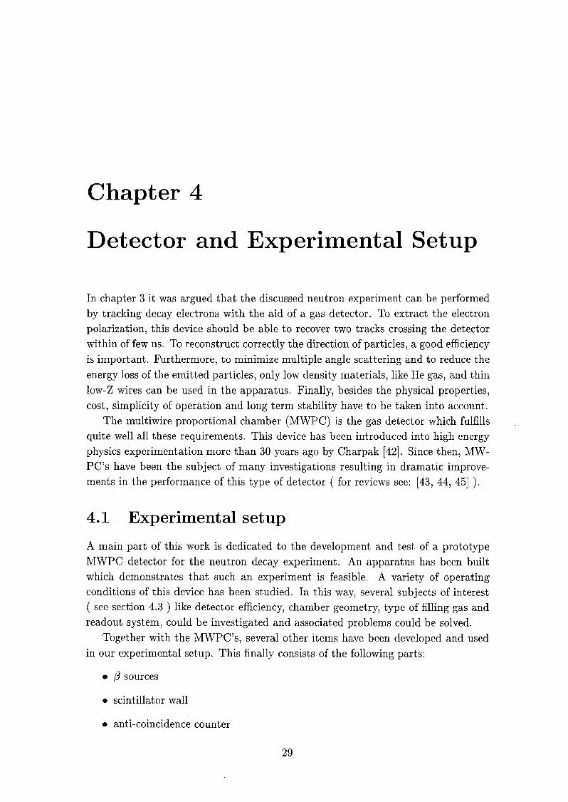
Figure 4.1 shows the two essentially different experimental conditions ( single
track and backscattering experiments ) for which the detection system has been
tested. For these two setups different responses of the chamber and much different
background conditions have been accepted. Both tests are very important to study
the performance of our equipment. While the backscattering setup was used to
simulate the neutron experiment, the single track configuration was very useful in
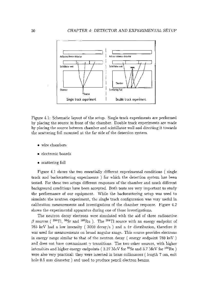
calibration measurements and investigations of the chamber response. Figure 4.2
shows the experimental apparatus during one of these investigations.
The neutron decay electrons were simulated with the aid of three radioactive
ß sources ( 204T1, 90Sr and 106Ru ). The 204T1 source with an energy endpoint of
765 keV had a low intensity ( 3000 decay/s ) and a An distribution, therefore it
was used for measurements on broad angular range. This source provides electrons
in energy range similar to that of the neutron decay ( energy endpoint 780 keV )and does not have contaminant 7 transitions. The two other sources, with higher
intensities and higher energy endpoints ( 2.27 MeV for 90Sr and 3.7 MeV for 106Ru )were also very practical: they were inserted in brass collimators ( length 7 cm, exit
hole 0.5 mm diameter ) and used to produce pencil electron beams.
4.1. EXPERIMENTAL SETUP 31
CIkhm!»«
IIV Cable
< 'ollimate
Sr soma'
PIVis
ISIectrtmîr
Boards
<<!atl»*Ml**H>
SOHlilh-tKl»!
Wall
Boards
(Anodes)
Figure 4.2: Photograph of the experimental apparatus. This setup is prepared
for a single track experiment. The collimated beam of electrons coming from the
90Sr source is placed in front of the chamber window. Electrons traversing the
chamber are stopped by the scintillator wall placed behind which triggers the data
acquisition system. The chamber pulses are processed by the electronic boards
mounted on the top and on the side.
32 CHAPTER 4: DETECTOR AND EXPERIMENTAL SETUP
During backscattering experiments the scattering foils were usually mounted
directly on the window of the chamber. We used 82Pb foils with a thickness of
17mg/cm2. Although the thickness of these foils is too large for the final experiment,
it permitted shorter data collecting times, which were necessary to study the variety
of operating conditions of the system.
The system of plastic scintillators measures the energy of the electrons and trig¬
gers the readout of the chamber signals. It consists of a row of three 15x5 cm2
rectangular scintillators with thickness 1 cm held together to build an active square
wall of 15 xl5 cm2. Along the short edges of every scintillator two photomultipliers
( PHILIPS XP2012B ) measure the produced light.
The size of the wall matches the active area of the MWPC and permits the
detection of almost all the electrons traversing the chamber. The 1 cm wall thickness
is well above the range of 780 keV electrons. However the more energetic particles as
cosmic ray muons will not be stopped in the wall. These particles, after traversing
the wall detector, are vetoed by an additional scintillator with the same thickness
and size as the wall, placed directly behind.
4.1.1 Chamber
Our chamber, which is shown on picture 4.3, is a sandwich construction of many
square 20x20 cm2 epoxy and stesalit planes of 1.6 mm and 3.0 mm thickness. A
central opening of 14x14 cm2 on every surface defines the active area of the detector.
The modular structure of this chamber permits easy modifications and it is
particularly well suited for optimization studies.
The electron trajectory is sampled by 4 MWPC planes inside the chamber. Every
plane is built out of two cathode planes with separate HV connectors and an anode
plane between them. The anode-cathode distance as well as the distance between
planes can be changed by varying the number of epoxy and stesalit frames between
them. The total width of the multi-planar chamber is in the order of 10 cm.
In order to enhance the transparency of the MWPC and reduce the scattering
of the ß particles, cathodes and anodes are made of thin wires of low-Z metals.
The electrode wires, placed every 4 mm, are directly soldered to the copper lines
of the epoxy planes. The wire spacing has been chosen according to the multiple
scattering of electrons ( see section 4.3 ) in He, giving a precision for the track angle
determination of a few degrees.
For every cell, 32 wires of the anode planes and 32 wires of one of the HV planes
( the active cathode ) are read out. This makes in total 256 active wires. While all
the anodes wires are horizontal, the cathode wires are mounted vertically. Therefore
the horizontal and vertical coordinates are retrieved by collecting the signals on the
cathodes, respectively the anodes.
4.1. EXPERIMENTAL SETUP 33
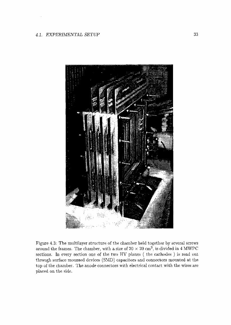
Figure 4.3: The multilayer structure of the chamber held together by several screws
around the frames. The chamber, with a size of 20 x 20 cm2, is divided in 4 MWPC
sections. In every section one of the two HV planes ( the cathodes ) is read out
through surface mounted devices (SMD) capacitors and connectors mounted at the
top of the chamber. The anode connectors with electrical contact with the wires are
placed on the side.
34 CHAPTER 4: DETECTOR AND EXPERIMENTAL SETUP
The anodes are of tungsten to provide the mechanical durability. On the cath¬
odes, having bigger wire diameters, 80%Ni/20%Cr wires could be mounted.
Using these geometrical parameters two chambers have been constructed: one
with 10 //m anode and 25 //m cathode wire diameter, and the other with 20 /mi
anode and 50 /zm cathode wire diameter.
After the optimization studies ( see section 4.3 ) a final asymmetric setup of the
chamber, where in every plane the gap between anode and cathodes is 1.6 mm for
the active cathode and 3.2 mm for the inactive ones, has been chosen. Furthermore
it has been shown that with a gas composition of Helium and methylal the chamber
can be operated in stable conditions.
4.2 Chamber readout electronics
In order to obtain a high detector efficiency and to avoid the ambiguity introduced
when multiple tracks are detected simultaneously, we developed a readout scheme
in which every wire is connected to its amplifier. In order to avoid a prohibitive cost
for a final detector, with more than 3000 wires, the readout system has been limited
to the simple identification of the firing wires.
In this scheme, ECL comparators at the output of the amplifiers transform the
analog signals into a logic 0 or 1. Every comparator is directly read out, in a time
window of 1 pis after the scintillator trigger, into a channel of a CAMAC TDC
module. The TDC time information is needed to adjust the time cuts ( see section
4.3.2 ) and it is used to tune the response time of the amplifiers. To detect the
energy of particles, the scintillator pulses are collected by CAMAC ADC modules.
This system has been working during the experiments with a trigger rate up to
1kHz.
It is known that mechanisms of signal formation for the anodes and cathodes
behave differently. In fact, while the primary avalanches are localized at the surface
of the firing anode wire, where the moving ions induce a signal of negative polarity,
opposite polarity signals are induced [46] at the neighboring electrodes. These two
effects cause a clean separation at the anodes ( see also figure 4.4 ) between firing and
neighboring wires.In the case of the cathodes there is no firing wire, and the signals
are spread around many wires. Despite of this, a similar electronic readout system
for cathodes and anodes, which is of great advantage in minimizing the efforts in
development and construction, is implemented in the chamber prototype.
A bipolar input amplifier ( LM6365, National Semiconductors ) has been adopted
to read out the wires with the same output polarity for both electrodes. Figure 4.5
shows the inverting and non-inverting electronic diagram circuits. The resulting
output pulses, seen in figure 4.4, have a half-width on the order of 300 ns and a
much faster rise-time ( in the order of 50 ns ).
4.2. CHAMBER READOUT ELECTRONICS
Cathode
200 ns
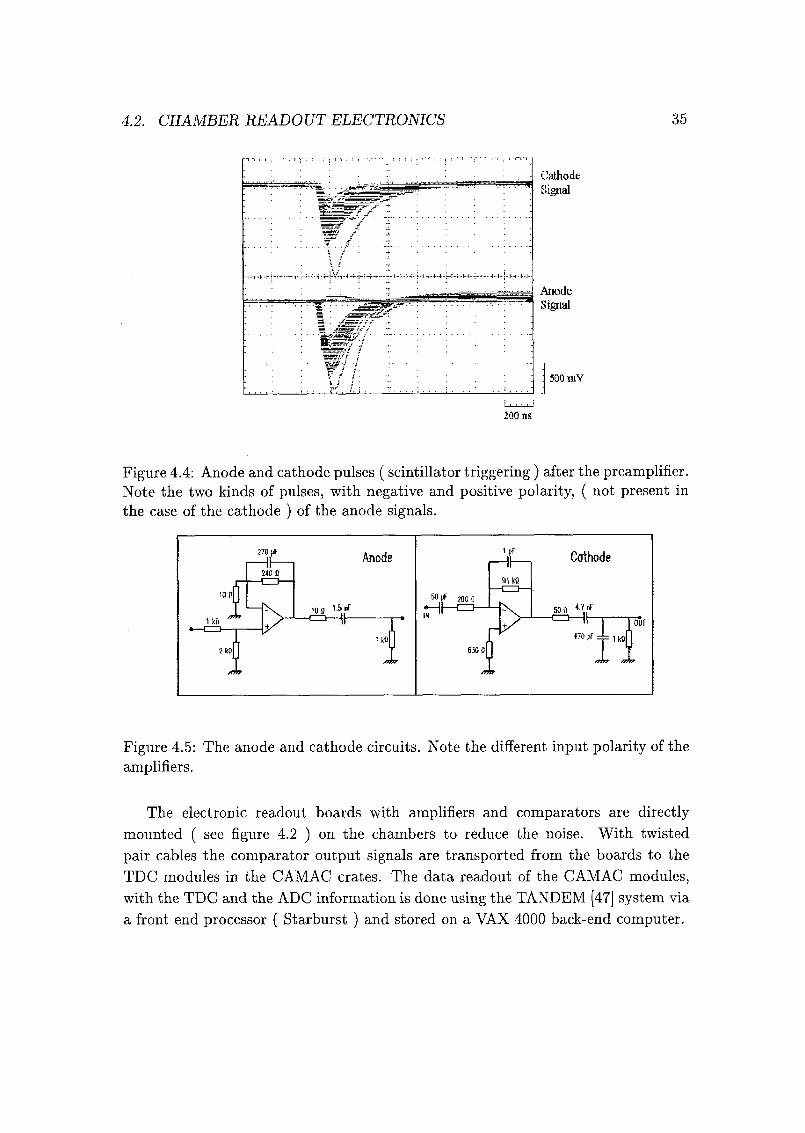
Figure 4.4: Anode and cathode pulses ( scintillator triggering ) after the preamplifier.Note the two kinds of pulses, with negative and positive polarity, ( not present in
the case of the cathode ) of the anode signals.
270 pf Anode
10 0 'fc/
1 pFCathode
son *\f
II
240 fl
50 pF m fl10 o[J
[S.
1k»"^ -\ iï"1' a -s
*/cm J) j
•
-0+/
'CPf4=1ko[J/zfa? /AW
5 4]K
63« of1k
Figure 4.5: The anode and cathode circuits. Note the different input polarity of the
amplifiers.
The electronic readout boards with amplifiers and comparators are directly
mounted ( see figure 4.2 ) on the chambers to reduce the noise. With twisted
pair cables the comparator output signals are transported from the boards to the
TDC modules in the CAMAC crates. The data readout of the CAMAC modules,
with the TDC and the ADC information is done using the TANDEM [47] system via
a front end processor ( Starburst ) and stored on a VAX 4000 back-end computer.
36 CHAPTER 4: DETECTOR AND EXPERIMENTAL SETUP
4.3 Experimental procedures and optimizations.
4.3.1 Gas mixture
To choose the optimal gas mixture of the chamber, not only the performance of
the detector has to be tested, but also energy loss and multiple Coulomb scattering
of the decay electrons have to be taken into account. For the neutron experiment
( electron kinetic energy between 200 and 700 keV ), we consider a 10% energy loss
and multiple scattering angles up to 15° as acceptable.
For homogeneous materials, the average energy loss AEk can be calculated with:
dEAEk = — - Ax (4.1)
where dE/dx is the mass stopping power and Ax is the target thickness. Stopping
power tables of electrons at several energies for various elements can be found in
[48]. For compounds and mixtures dE/dx can be calculated from [49]:
dE dE dEtt
.
—- =w1— +w2— +... (4.2)ax mix ax i dx 2
where Wi, the fraction by weight of the element i with number of atoms a^ and
atomic weight A{, is given by:
A good approximation for the angular distribution of electrons after traversing
materials can be obtained with the method of Molière [50]. The effects of multiple
scattering are characterized by the R.M.S. angle 'Orms- The planar projection 9RMs
[rad], calculated according to [7], is given by:
Brms = 13'6^eV jAx/Xo • (1 + 0.0038 • ln{Ax/X0)) (4.4)
where ß and p is the electron speed and momentum respectively, and Ax, X0 are
the thickness and the radiation length of the material. Values of Xq for few elements
are tabulated in ref. [7]. For a compound or a mixture, analog to (4.2), we have
[49]:111—
=wx— +w2— +.-. (4.5)^Omix ^-0 1 ^-0 2
where Wi is given by (4.3).
4.3. EXPERIMENTAL PROCEDURES AND OPTIMIZATIONS. 37
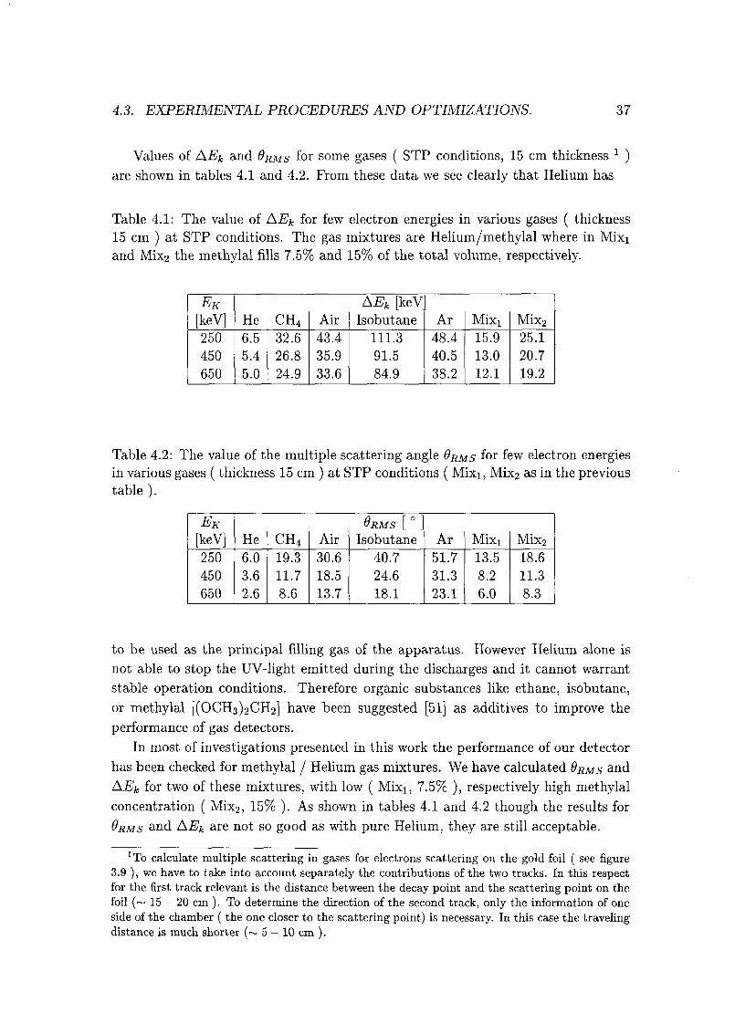
Values of AEk and 9rms for some gases ( STP conditions, 15 cm thickness 1 )
are shown in tables 4.1 and 4.2. From these data we see clearly that Helium has
Table 4.1: The value of AEk for few electron energies in various gases ( thickness
15 cm ) at STP conditions. The gas mixtures are Helium/methylal where in Mixi
and Mix2 the methylal fills 7.5% and 15% of the total volume, respectively.
Ek
[keV] He CH4 Air
AEk [keVIsobutane Ar Mixi Mix2
250
450
650
6.5
5.4
5.0
32.6
26.8
24.9
43.4
35.9
33.6
111.3
91.5
84.9
48.4
40.5
38.2
15.9
13.0
12.1
25.1
20.7
19.2
Table 4.2: The value of the multiple scattering angle Brms f°r few electron energiesin various gases ( thickness 15 cm ) at STP conditions ( Mixi, Mix2 as in the previoustable ).
Ek
[keV] He CH4 Air
Qrms [°
.
Isobutane Ar Mixx Mix2
250
450
650
6.0
3.6
2.6
19.3
11.7
8.6
30.6
18.5
13.7
40.7
24.6
18.1
51.7
31.3
23.1
13.5
8.2
6.0
18.6
11.3
8.3
to be used as the principal filling gas of the apparatus. However Helium alone is
not able to stop the UV-light emitted during the discharges and it cannot warrant
stable operation conditions. Therefore organic substances like ethane, isobutane,
or methylal [(OCH3)2CH2] have been suggested [51] as additives to improve the
performance of gas detectors.
In most of investigations presented in this work the performance of our detector
has been checked for methylal / Helium gas mixtures. We have calculated 9rms and
AEk for two of these mixtures, with low ( Mix1; 7.5% ), respectively high methylal
concentration ( Mix2, 15% ). As shown in tables 4.1 and 4.2 though the results for
9Rms and AEk are not so good as with pure Helium, they are still acceptable.
xTo calculate multiple scattering in gases for electrons scattering on the gold foil ( see figure3.9 ), we have to take into account separately the contributions of the two tracks. In this respectfor the first track relevant is the distance between the decay point and the scattering point on the
foil (~ 15 — 20 cm ). To determine the direction of the second track, only the information of one
side of the chamber ( the one closer to the scattering point) is necessary. In this case the travelingdistance is much shorter (~ 5 — 10 cm ).
38 CHAPTER 4: DETECTOR AND EXPERIMENTAL SETUP
Lü
>>O
c
CD
CD
Oc
<
0.95
0.9
0.85
Breakdown Breakdown
OGas Mixture: 92.5% He, 7.5% Methylal
• Gas Mixture: 90 % He, 10 % MethylalDGas Mixture: 87.5% He, 12.5% Methylal
Gas Mixture: 85 % He, 15 % Methylal
2.2 2.4 2.6 2.8
Voltage (kV)
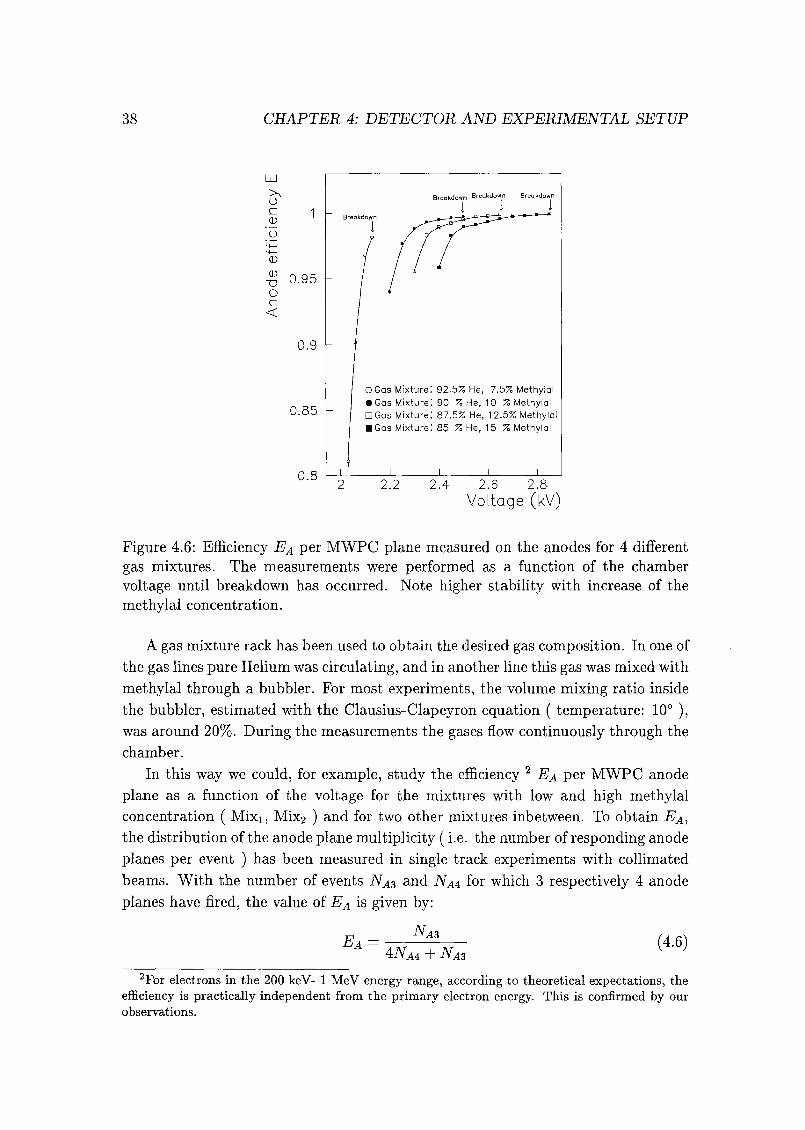
Figure 4.6: Efficiency Ea per MWPC plane measured on the anodes for 4 different
gas mixtures. The measurements were performed as a function of the chamber
voltage until breakdown has occurred. Note higher stability with increase of the
methylal concentration.
A gas mixture rack has been used to obtain the desired gas composition. In one of
the gas lines pure Helium was circulating, and in another line this gas was mixed with
methylal through a bubbler. For most experiments, the volume mixing ratio inside
the bubbler, estimated with the Clausius-Clapeyron equation ( temperature: 10° ),was around 20%. During the measurements the gases flow continuously through the
chamber.
In this way we could, for example, study the efficiency2Ea per MWPC anode
plane as a function of the voltage for the mixtures with low and high methylal
concentration ( Mixi, Mix2 ) and for two other mixtures inbetween. To obtain Ea,
the distribution of the anode plane multiplicity ( i.e. the number of responding anode
planes per event ) has been measured in single track experiments with collimated
beams. With the number of events Nas and NA4 for which 3 respectively 4 anode
planes have fired, the value of Ea is given by:
NA3Ea
ANA4 + NA3
(4.6)
2 For electrons in the 200 keV- 1 MeV energy range, according to theoretical expectations, the
efficiency is practically independent from the primary electron energy. This is confirmed by our
observations.

4.3. EXPERIMENTAL PROCEDURES AND OPTIMIZATIONS. 39
* 4
O
X
C/l-,
c
D
O
°2
1
5 10 15 20
Hit multiplicity H
Figure 4.7: The anode hit multiplicity measured with the Tl source ( wide angularacceptance ), and the TDC time distribution of the collected anode hits. If a cut in
the time window is used, a narrow hit distribution ( shadowed spectrum ) is obtained
by rejecting hits which arrive at the electrode later than 300 ns after the scintillator
trigger pulse. The efficiency per plane, 0.985 and 0.975 for the data without and
with timing cuts respectively, changes only very little.
Figure 4.6 shows the efficiency curves measured as a function of the voltage until
a breakdown has happened in the detector. It is evident that it is more difficult to
obtain a fully efficient chamber if a small amount of methylal is used in the chamber.
However, for a methylal concentration above 10%, a good efficiency can be obtained
for a large range of the applied high voltage.In conclusion, these results show that it is possible to operate the chamber in
stable conditions while using gas mixtures with acceptable energy loss and multipleCoulomb scattering effects.
4.3.2 Anode hit multiplicity and time window
Another quantity measured during the tests was the distribution of the total number
of hits Ha, He per event on the four anodes, respectively cathodes. In single track
experiments, the ideal situation for a track reconstruction arises when only one wire
per plane responds, namely the one which is closest located to the primary ion
charges. Such a chamber response is difficult to realize, especially if the electron
trajectory is not orthogonal to the chamber planes. Moreover, in our case, the hit
multiplicity of the chamber has to be minimal for a wide angular acceptance, with
an efficiency per plane higher than 90%.
We performed several experiments to study this problem using the uncollimated
1» 25O
x2
« 1 5c
3 1O
"05
0
1) 02 04
1 '>_
06 08
time (fMs)
i
40 CHAPTER 4: DETECTOR AND EXPERIMENTAL SETUP
Tl source to obtain various track inclinations at the same time. A noticeable im¬
provement in the hit multiplicity per event in the case of anodes has been obtained
by adjusting the length of the time gate after the scintillator trigger for the collection
of the anode signals. Figure 4.7 shows the effect: by cutting away the latest part
( ~ 10%o ) of the anode time spectrum the hit multiplicity is substantially improved.
The obtained spectrum is close to the ideal one of one fire on each plane and it is
certainly good enough to perform the reconstruction of the tracks.
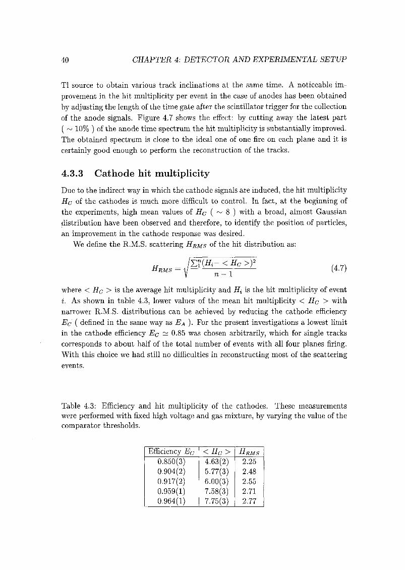
4.3.3 Cathode hit multiplicity
Due to the indirect way in which the cathode signals are induced, the hit multiplicity
He of the cathodes is much more difficult to control. In fact, at the beginning of
the experiments, high mean values of Hc ( ~ 8 ) with a broad, almost Gaussian
distribution have been observed and therefore, to identify the position of particles,
an improvement in the cathode response was desired.
We define the R.M.S. scattering HRMS of the hit distribution as:
Hrms =/E?W- <Bc »1 (4.7)
y n — 1
where < He > is the average hit multiplicity and Hi is the hit multiplicity of event
i. As shown in table 4.3, lower values of the mean hit multiplicity < He > with
narrower R.M.S. distributions can be achieved by reducing the cathode efficiency
Ec ( defined in the same way as Ea ) For the present investigations a lowest limit
in the cathode efficiency Ec —
0.85 was chosen arbitrarily, which for single tracks
corresponds to about half of the total number of events with all four planes firing.
With this choice we had still no difficulties in reconstructing most of the scattering
events.
Table 4.3: Efficiency and hit multiplicity of the cathodes. These measurements
were performed with fixed high voltage and gas mixture, by varying the value of the
comparator thresholds.
Efficiency Ec <HC> Hrms
0.850(3) 4.63(2) 2.25
0.904(2) 5.77(3) 2.48
0.917(2) 6.00(3) 2.55
0.959(1) 7.58(3) 2.71
0.964(1) 7.75(3) 2.77
4.3. EXPERIMENTAL PROCEDURES AND OPTIMIZATIONS. 41
OT1200
c
O1000ü
800
600
400
200
0
Mean : 4.40
R.M.S: 2.21
10 20
Hit multiplicity H
£3000 _ Efficiency E=0.865(4)
O
ü2500 -
2000 -
1500 -
1000
500
n
12 3 4
Plane multiplicity
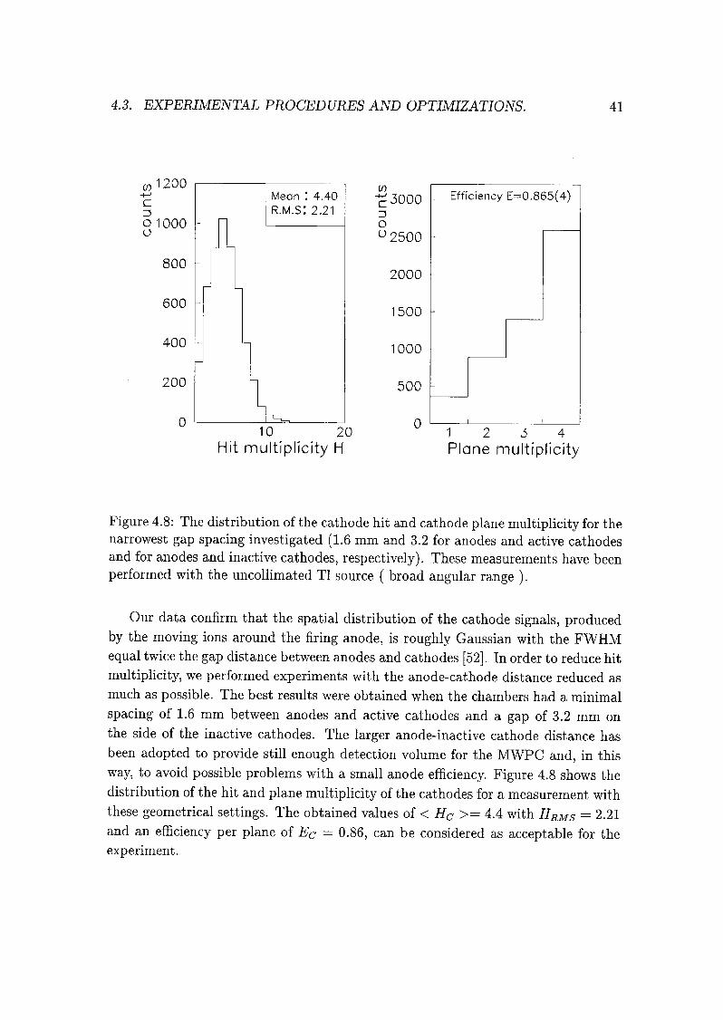
Figure 4.8: The distribution of the cathode hit and cathode plane multiplicity for the
narrowest gap spacing investigated (1.6 mm and 3.2 for anodes and active cathodes
and for anodes and inactive cathodes, respectively). These measurements have been
performed with the uncollimated Tl source ( broad angular range ).
Our data confirm that the spatial distribution of the cathode signals, produced
by the moving ions around the firing anode, is roughly Gaussian with the FWHM
equal twice the gap distance between anodes and cathodes [52]. In order to reduce hit
multiplicity, we performed experiments with the anode-cathode distance reduced as
much as possible. The best results were obtained when the chambers had a minimal
spacing of 1.6 mm between anodes and active cathodes and a gap of 3.2 mm on
the side of the inactive cathodes. The larger anode-inactive cathode distance has
been adopted to provide still enough detection volume for the MWPC and, in this
way, to avoid possible problems with a small anode efficiency. Figure 4.8 shows the
distribution of the hit and plane multiplicity of the cathodes for a measurement with
these geometrical settings. The obtained values of < Hc >= 4.4 with HRMs = 2.21
and an efficiency per plane of Ec = 0.86, can be considered as acceptable for the
experiment.
42 CHAPTER 4: DETECTOR AND EXPERIMENTAL SETUP
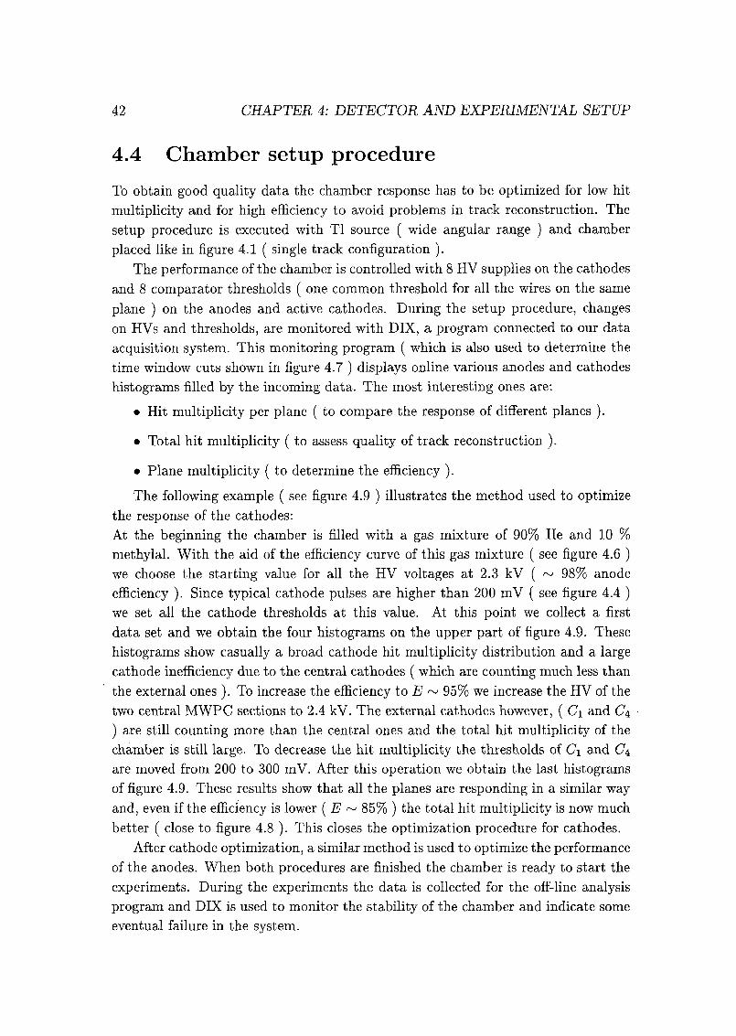
4.4 Chamber setup procedure
To obtain good quality data the chamber response has to be optimized for low hit
multiplicity and for high efficiency to avoid problems in track reconstruction. The
setup procedure is executed with Tl source ( wide angular range ) and chamber
placed like in figure 4.1 ( single track configuration ).The performance of the chamber is controlled with 8 HV supplies on the cathodes
and 8 comparator thresholds ( one common threshold for all the wires on the same
plane ) on the anodes and active cathodes. During the setup procedure, changes
on HVs and thresholds, are monitored with DIX, a program connected to our data
acquisition system. This monitoring program ( which is also used to determine the
time window cuts shown in figure 4.7 ) displays online various anodes and cathodes
histograms filled by the incoming data. The most interesting ones are:
• Hit multiplicity per plane ( to compare the response of different planes ).
• Total hit multiplicity ( to assess quality of track reconstruction ).
• Plane multiplicity ( to determine the efficiency ).
The following example ( see figure 4.9 ) illustrates the method used to optimize
the response of the cathodes:
At the beginning the chamber is filled with a gas mixture of 90% He and 10 %
methylal. With the aid of the efficiency curve of this gas mixture ( see figure 4.6 )we choose the starting value for all the HV voltages at 2.3 kV ( ~ 98% anode
efficiency ). Since typical cathode pulses are higher than 200 mV ( see figure 4.4 )we set all the cathode thresholds at this value. At this point we collect a first
data set and we obtain the four histograms on the upper part of figure 4.9. These
histograms show casually a broad cathode hit multiplicity distribution and a large
cathode inefficiency due to the central cathodes ( which are counting much less than
the external ones ). To increase the efficiency to E ~ 95% we increase the HV of the
two central MWPC sections to 2.4 kV. The external cathodes however, ( C\ and C±
) are still counting more than the central ones and the total hit multiplicity of the
chamber is still large. To decrease the hit multiplicity the thresholds of C\ and C$
are moved from 200 to 300 mV. After this operation we obtain the last histograms
of figure 4.9. These results show that all the planes are responding in a similar way
and, even if the efficiency is lower ( E ~ 85% ) the total hit multiplicity is now much
better ( close to figure 4.8 ). This closes the optimization procedure for cathodes.
After cathode optimization, a similar method is used to optimize the performance
of the anodes. When both procedures are finished the chamber is ready to start the
experiments. During the experiments the data is collected for the off-line analysis
program and DIX is used to monitor the stability of the chamber and indicate some
eventual failure in the system.
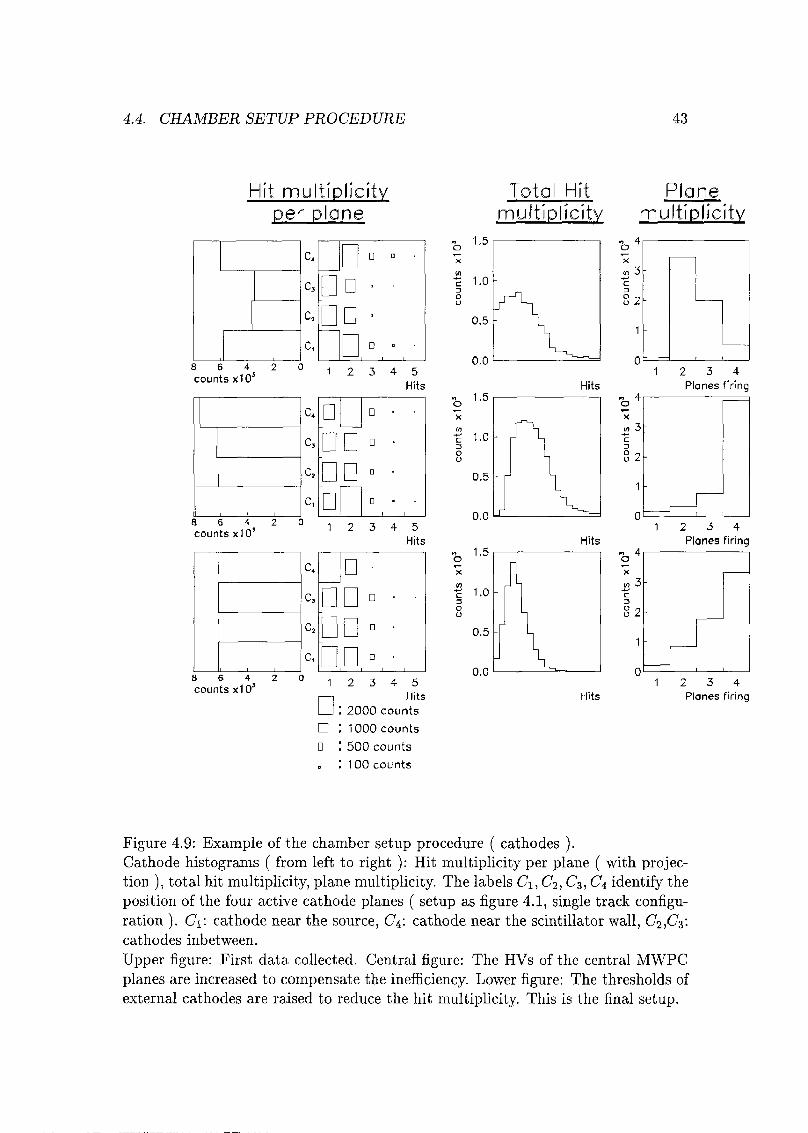
4.4. CHAMBER SETUP PROCEDURE 43
Hit multiplicity
per plane
8 6 4 2
counts x103
8 6 4 2 0
counts x103
i . i
8 6 4 2 0
counts x10*
c3
c2
c,
Da
Dû0
i i i
12 3 4 5
Hits
DD °
DD
nn°12 3 4 5
Hits
c4 a •
c3 DD» •
c2 DD"c, DD»12 3 4 5
I—!Hits
I I : 2000 counts
: 1000 counts
D : 500 counts
, ! 100 counts
Total Hit
multiplicity
Plane
0.0
o
x
Hits
1.0 -
Jl
0.5 -
r
n n
Hits
r
b4
Till Itiplicity
X
«î 3
c
o 2.
1
01 2 3 4
°4X
tn 3
c
D
on
o 1
Planes firing
-
1 -
0 ,
1 2 3 4
24X
n 3-t-.
c
ü 2
Planes firing
-
1 -
0,
1 2 3 4
Planes firing
Figure 4.9: Example of the chamber setup procedure ( cathodes ).Cathode histograms ( from left to right ): Hit multiplicity per plane ( with projec¬tion ), total hit multiplicity, plane multiplicity. The labels Cx, C2, C3, C4 identify the
position of the four active cathode planes ( setup as figure 4.1, single track configu¬ration ). C\. cathode near the source, C4: cathode near the scintillator wall, C2,C3:cathodes inbetween.
Upper figure: First data collected. Central figure: The HVs of the central MWPC
planes are increased to compensate the inefficiency. Lower figure: The thresholds of
external cathodes are raised to reduce the hit multiplicity. This is the final setup.
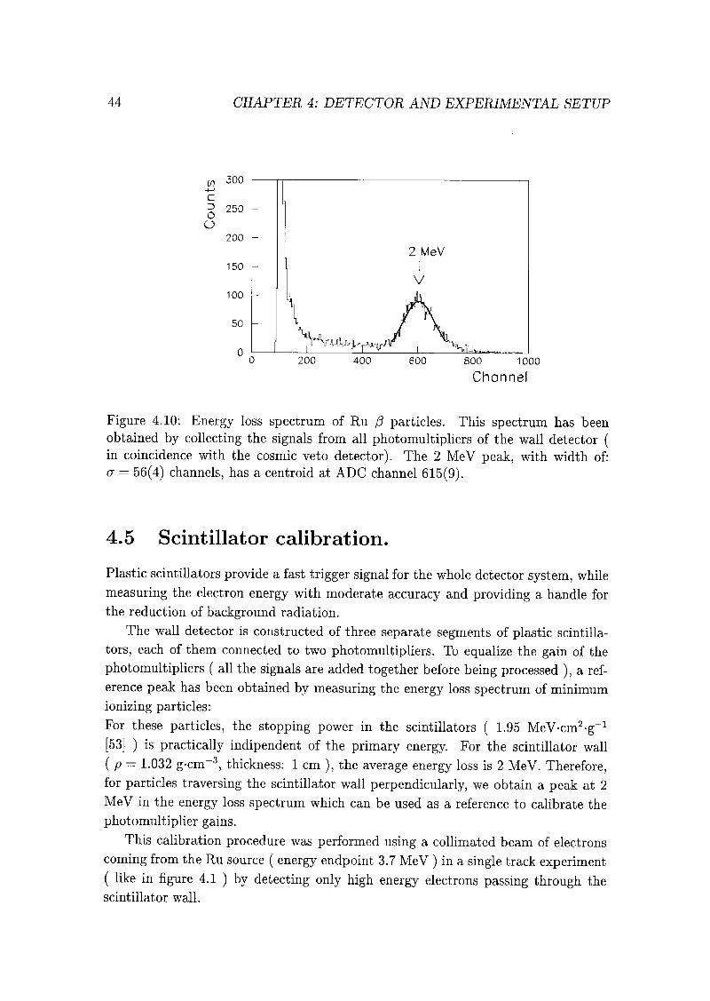
44 CHAPTER 4: DETECTOR AND EXPERIMENTAL SETUP
300
800 1000
Channel
Figure 4.10: Energy loss spectrum of Ru ß particles. This spectrum has been
obtained by collecting the signals from all photomultipliers of the wall detector (in coincidence with the cosmic veto detector). The 2 MeV peak, with width of:
a = 56(4) channels, has a centroid at ADC channel 615(9).
4.5 Scintillator calibration.
Plastic scintillators provide a fast trigger signal for the whole detector system, while
measuring the electron energy with moderate accuracy and providing a handle for
the reduction of background radiation.
The wall detector is constructed of three separate segments of plastic scintilla¬
tors, each of them connected to two photomultipliers. To equalize the gain of the
photomultipliers ( all the signals are added together before being processed ), a ref¬
erence peak has been obtained by measuring the energy loss spectrum of minimum
ionizing particles:
For these particles, the stopping power in the scintillators ( 1.95 MeV-cm2-g_1[53] ) is practically indipendent of the primary energy. For the scintillator wall
( p— 1.032 g-cm~3, thickness: 1 cm ), the average energy loss is 2 MeV. Therefore,
for particles traversing the scintillator wall perpendicularly, we obtain a peak at 2
MeV in the energy loss spectrum which can be used as a reference to calibrate the
photomultiplier gains.
This calibration procedure was performed using a collimated beam of electrons
coming from the Ru source ( energy endpoint 3.7 MeV ) in a single track experiment
( like in figure 4.1 ) by detecting only high energy electrons passing through the
scintillator wall.
4.5. SCINTILLATOR CALIBRATION. Ab
m 8000
200 400 800 1000
Channel
800 1000
Channel
Figure 4.11: Sr and Tl /3-spectra. Upper histogram: Tl, lower histogram: Sr. For
each distribution, the endpoint of the /3-spectrum has been determined by fittingthe high energy part of the spectrum with (4.8). The calculated endpoint channel
numbers are: Emax(Tl) ->• 285(10), Emax{Sr) -> 726(24). The distortion of the
spectra at low energies is due to discrimination thresholds.
To detect these electrons the scintillator wall was set in coincidence with the
cosmic ray veto detector. The measured spectrum is shown in figure 4.10. To obtain
the energy calibration point at 2 MeV we fitted the spectrum with a Gaussian curve.
The observed pulse height resolution of the scintillator is around 15%.
Other two reference points have been obtained by determining the ADC con¬
version value corresponding to the energy endpoint of the Sr and Tl /5-spectra ( an
example of the measurement and analysis of these spectra is described in chapter
5.2 ). This was possible since in this case all the electrons emitted from the source
are stopped inside the scintillator and the full ß spectrum could be measured. The
ADC conversion value corresponding to these two reference points has been deter¬
mined by fitting the high energy part of each distribution with the following function
derived from the equation (3.1) of the /3-decay energy spectrum:
F(X) = Pz-{Ek-Me)2-{Emax-Ekf
Ek = P1-X + P2
(4.8)
(4.9)
where X is the channel number, Ek is the kinetic energy of the particles and Me is
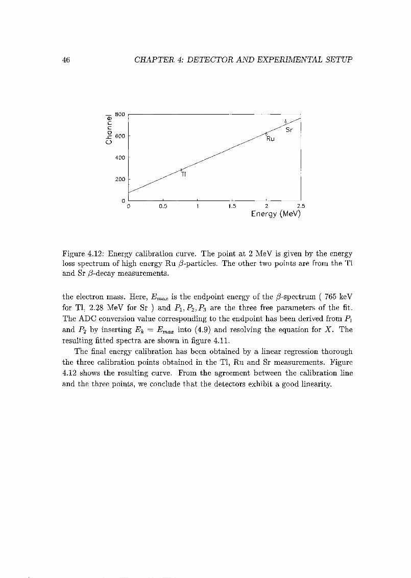
46 CHAPTER 4: DETECTOR AND EXPERIMENTAL SETUP
— 8000>
c
c
_C 600
Ü
400
200
0
0 0.5 1 1.5 2 2.5
Energy (MeV)
Figure 4.12: Energy calibration curve. The point at 2 MeV is given by the energy
loss spectrum of high energy Ru /3-particles. The other two points are from the Tl
and Sr /3-decay measurements.
the electron mass. Here, Emax is the endpoint energy of the /3-spectrum ( 765 keV
for Tl, 2.28 MeV for Sr ) and Pi,P2,Ps are the three free parameters of the fit.
The ADC conversion value corresponding to the endpoint has been derived from Pi
and P2 by inserting Ek = Emax into (4.9) and resolving the equation for X. The
resulting fitted spectra are shown in figure 4.11.
The final energy calibration has been obtained by a linear regression thorough
the three calibration points obtained in the Tl, Ru and Sr measurements. Figure
4.12 shows the resulting curve. From the agreement between the calibration line
and the three points, we conclude that the detectors exhibit a good linearity.
Chapter 5
Data Analysis
5.1 Data structure and general concept
The data files are collected as a sequence of records. Each record corresponds to a
trigger of the data acquisition system. The structure of these records consists of a
field for the pulse height ADC information of the scintillator wall ( 10 bits ) and
8 other fields which identify planes and firing chamber wires ( 8 x 32 bits ). Other
details, like time information available for online diagnostics, are not recorded. Nev¬
ertheless the stored information is sufficient to permit a complex analysis, including
multiple filters and track reconstruction.
The records can be subdivided in the following groups:
• Zero hits : records for which no chamber wire was firing ( only scintillator
pulse height recorded ).
• Anode ( cathode ) track candidates : records for which the anode ( cathode )
plane multiplicity is > 3.
• Events : records for which tracking has been successfully performed. This kind
of records represents charged particles which were traversing the chamber.
A program ( NIX ), consisting of a set of PAW [54] commands and FORTRAN
routines, has been developed to analyze the data files. The general concept is the
following:
• Every operation executed with NIX (histogram display, data filtering, track
reconstruction ) is based on a subset of the initial records.
• Histograms are filled by calculating for each record of the actual set the value
of the histogram variable. For example, the hit multiplicity histograms are
filled by counting the number of firing wires in each recorded trigger.
47
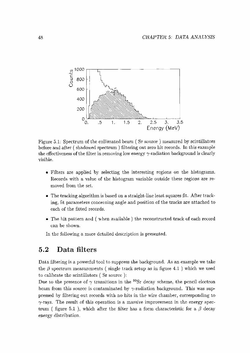
48 CHAPTER 5: DATA ANALYSIS
w1000
|-|r
| 800 - \
0. .5 1. 1.5 2. 2.5 3. 3.5
Energy (MeV)
Figure 5.1: Spectrum of the collimated beam ( Sr source ) measured by scintillators
before and after ( shadowed spectrum ) filtering out zero hit records. In this examplethe effectiveness of the filter in removing low energy 7-radiation background is clearly
visible.
• Filters are applied by selecting the interesting regions on the histograms.
Records with a value of the histogram variable outside these regions are re¬
moved from the set.
• The tracking algorithm is based on a straight-line least squares fit. After track¬
ing, fit parameters concerning angle and position of the tracks are attached to
each of the fitted records.
• The hit pattern and ( when available ) the reconstructed track of each record
can be shown.
In the following a more detailed description is presented.
5.2 Data filters
Data filtering is a powerful tool to suppress the background. As an example we take
the ß spectrum measurements ( single track setup as in figure 4.1 ) which we used
to calibrate the scintillators ( Sr source ):Due to the presence of 7 transitions in the 90Sr decay scheme, the pencil electron
beam from this source is contaminated by 7-radiation background. This was sup¬
pressed by filtering out records with no hits in the wire chamber, corresponding to
7-rays. The result of this operation is a massive improvement in the energy spec¬
trum ( figure 5.1 ), which after the filter has a form characteristic for a ß decay
energy distribution.
5.3. FITTING ROUTINE 49
Another filter is commonly used before track reconstruction. This filter selects
records from the measurement files, with at least three points available for tracking.
A last group of filters is applied on events and uses the geometrical information
obtained during track reconstruction. For example, a filter of this kind, used in
backscattering experiments, selects events with scattering angle ê < 165° between
the two tracks. This improves a determination of the position of the scattering foil
and of the wire planes ( see chapter 6.5, figure 6.11 ).
5.3 Fitting routine
After removing most of the background with preliminary filters, the data is passed
through the fitting routine. The input parameters required by this procedure are
distances between the chamber planes and window, position of the source, position of
the scintillator wall and, in the case of backscattering experiments, size and position
of the scattering foil.
The most probable electron trajectories are found by two independent planar
least square fit reconstructions of the track for anodes ( vertical projection ) and
cathodes ( horizontal projection ). The fits are performed only if at least three
wire planes in each projection have fired. Due to the high detector efficiency ( see
chapter 4.3 ), this requirement can be easily reached for most of the electrons travers¬
ing the chamber.
Before fitting, adjacent hits are grouped into clusters. The fit is then executed
in several steps. In case of single track events, to eliminate spurious hits, a two-
step fit has been adopted ( see fig. 5.2 ): In the first phase the preliminary fit-line
is calculated by taking into account exclusively planes with single clusters. Then,
for planes with more clusters, only the cluster closest to the preliminary fit-line is
selected for the final tracking. The other clusters, considered as spurious hits, are
eliminated. In the last iteration a new straight line is fitted through the hit patterns
corresponding to the selected track clusters.
For double tracks the first question is to find out which cluster belongs to which
track. In case of clean backscattering events we expect a F-pattern with the vertex
in the vicinity of the foil and, in a simple case, exactly two clusters on each chamber
plane. We identify the clusters belonging to a track by a condition that they are all
on the same side of the detector. After this, to eliminate spurious hits and performthe fits we proceed similar as in the single track case.
The quality of the fit procedure has been estimated with a visual check. 1 In the
single track case, an experiment with Tl source has been analyzed for this purpose.
:For a data set, the hit pattern and the reconstructed track of each record has been examined.
In more than 95% of cases the records could be classified ( successful cases, fit failures, ...) without
ambiguity.
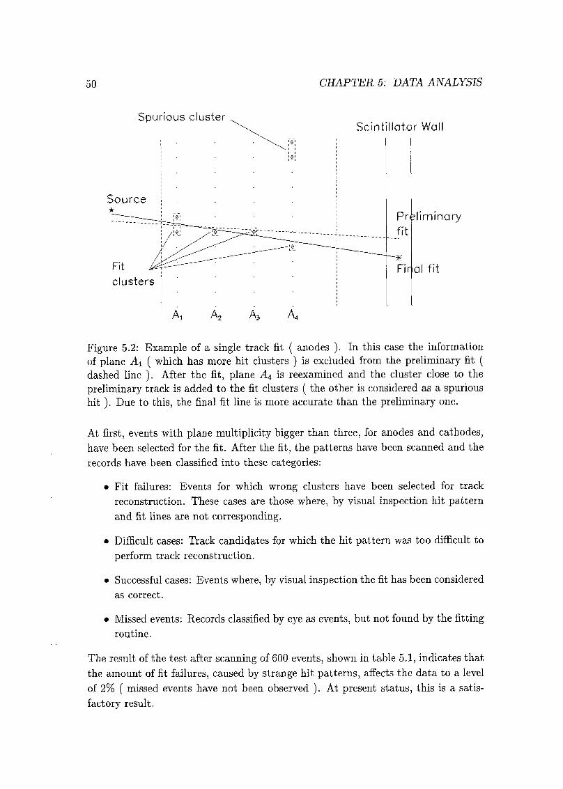
50 CHAPTER 5: DATA ANALYSIS
Spurious clusterScintillator Wal
Fit
clusters
liminary
Firal fit
Figure 5.2: Example of a single track fit ( anodes ). In this case the information
of plane A4 ( which has more hit clusters ) is excluded from the preliminary fit (dashed line ). After the fit, plane A4 is reexamined and the cluster close to the
preliminary track is added to the fit clusters ( the other is considered as a spurious
hit ). Due to this, the final fit line is more accurate than the preliminary one.
At first, events with plane multiplicity bigger than three, for anodes and cathodes,
have been selected for the fit. After the fit, the patterns have been scanned and the
records have been classified into these categories:
• Fit failures: Events for which wrong clusters have been selected for track
reconstruction. These cases are those where, by visual inspection hit pattern
and fit lines are not corresponding.
• Difficult cases: Track candidates for which the hit pattern was too difficult to
perform track reconstruction.
• Successful cases: Events where, by visual inspection the fit has been considered
as correct.
• Missed events: Records classified by eye as events, but not found by the fitting
routine.
The result of the test after scanning of 600 events, shown in table 5.1, indicates that
the amount of fit failures, caused by strange hit patterns, affects the data to a level
of 2% ( missed events have not been observed ). At present status, this is a satis¬
factory result.
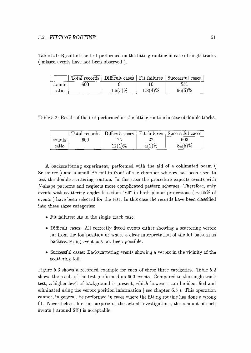
5.3. FITTING ROUTINE 51
Table 5.1: Result of the test performed on the fitting routine in case of single tracks
( missed events have not been observed ).
Total records Difficult cases Fit failures Successful cases
counts
ratio
600 9
1.5(5)%
10
1.3(4)%
581
96(5)%
Table 5.2: Result of the test performed on the fitting routine in case of double tracks.
Total records Difficult cases Fit failures Successful cases
counts
ratio
600 75
12(1)%
22
4(1)%
503
84(5)%
A backscattering experiment, performed with the aid of a collimated beam (Sr source ) and a small Pb foil in front of the chamber window has been used to
test the double scattering routine. In this case the procedure expects events with
F-shape patterns and neglects more complicated pattern schemes. Therefore, only
events with scattering angles less than 160° in both planar projections ( ~ 65% of
events ) have been selected for the test. In this case the records have been classified
into these three categories:
• Fit failures: As in the single track case.
• Difficult cases: All correctly fitted events either showing a scattering vertex
far from the foil position or where a clear interpretation of the hit pattern as
backscattering event has not been possible.
• Successful cases: Backscattering events showing a vertex in the vicinity of the
scattering foil.
Figure 5.3 shows a recorded example for each of these three categories. Table 5.2
shows the result of the test performed on 600 events. Compared to the single track
test, a higher level of background is present, which however, can be identified and
eliminated using the vertex position information ( see chapter 6.5 ). This operation
cannot, in general, be performed in cases where the fitting routine has done a wrong
fit. Nevertheless, for the purpose of the actual investigations, the amount of such
events ( around 5%) is acceptable.
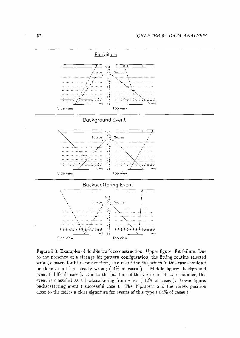
52 CHAPTER 5: DATA ANALYSIS
Fit failure
Side view
Background Event
Source
(cm)
Side view Top view
Backscattering Event
(cm)
view
Figure 5.3: Examples of double track reconstruction. Upper figure: Fit failure. Due
to the presence of a strange hit pattern configuration, the fitting routine selected
wrong clusters for fit reconstruction, as a result the fit ( which in this case shouldn't
be done at all ) is clearly wrong ( 4% of cases ) .Middle figure: background
event ( difficult case ). Due to the position of the vertex inside the chamber, this
event is classified as a backscattering from wires ( 12% of cases ). Lower figure:
backscattering event ( successful case ). The F-pattern and the vertex positionclose to the foil is a clear signature for events of this type ( 84% of cases ).
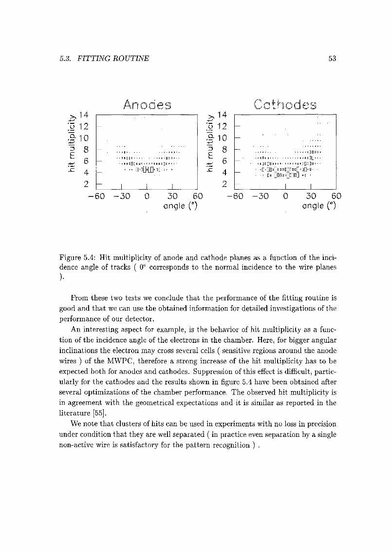
5.3. FITTING ROUTINE 53
>>14
S 12
£108
6
4
2
D
En BD D • * • • i • DD D
d ii n[]0 n a " ' ' "D d n nQn « •
"öG"[TJ"DD
>J4
'g 12
•1108
6
4
E
-60 -30 0 30 60
angle (°)
iDDat
Dan i.idQ[]m
D DD QD n B .g afjDDD " '
•D'DD»D»nDllDOnDQ.DD'D-d« Dodd.Qdddd »
-60 -30 0 30 60
angle (°)
Figure 5.4: Hit multiplicity of anode and cathode planes as a function of the inci¬
dence angle of tracks ( 0° corresponds to the normal incidence to the wire planes
)•
From these two tests we conclude that the performance of the fitting routine is
good and that we can use the obtained information for detailed investigations of the
performance of our detector.
An interesting aspect for example, is the behavior of hit multiplicity as a func¬
tion of the incidence angle of the electrons in the chamber. Here, for bigger angular
inclinations the electron may cross several cells ( sensitive regions around the anode
wires ) of the MWPC, therefore a strong increase of the hit multiplicity has to be
expected both for anodes and cathodes. Suppression of this effect is difficult, partic¬
ularly for the cathodes and the results shown in figure 5.4 have been obtained after
several optimizations of the chamber performance. The observed hit multiplicity is
in agreement with the geometrical expectations and it is similar as reported in the
literature [55].We note that clusters of hits can be used in experiments with no loss in precision
under condition that they are well separated ( in practice even separation by a single
non-active wire is satisfactory for the pattern recognition ) .

54 CHAPTER 5: DATA ANALYSIS
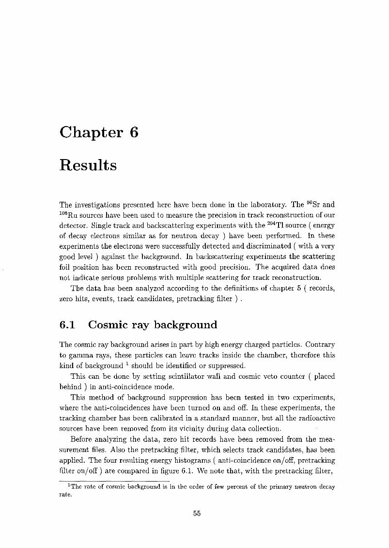
Chapter 6
Results
The investigations presented here have been done in the laboratory. The 90Sr and
106Ru sources have been used to measure the precision in track reconstruction of our
detector. Single track and backscattering experiments with the 204T1 source ( energyof decay electrons similar as for neutron decay ) have been performed. In these
experiments the electrons were successfully detected and discriminated ( with a very
good level ) against the background. In backscattering experiments the scattering
foil position has been reconstructed with good precision. The acquired data does
not indicate serious problems with multiple scattering for track reconstruction.
The data has been analyzed according to the definitions of chapter 5 ( records,
zero hits, events, track candidates, pretracking filter ) .
6.1 Cosmic ray background
The cosmic ray background arises in part by high energy charged particles. Contrary
to gamma rays, these particles can leave tracks inside the chamber, therefore this
kind of background* should be identified or suppressed.
This can be done by setting scintillator wall and cosmic veto counter ( placed
behind ) in anti-coincidence mode.
This method of background suppression has been tested in two experiments,
where the anti-coincidences have been turned on and off. In these experiments, the
tracking chamber has been calibrated in a standard manner, but all the radioactive
sources have been removed from its vicinity during data collection.
Before analyzing the data, zero hit records have been removed from the mea¬
surement files. Also the pretracking filter, which selects track candidates, has been
applied. The four resulting energy histograms ( anti-coincidence on/off, pretracking
filter on/off ) are compared in figure 6.1. We note that, with the pretracking filter,
1The rate of cosmic background is in the order of few percent of the primary neutron decayrate.
55
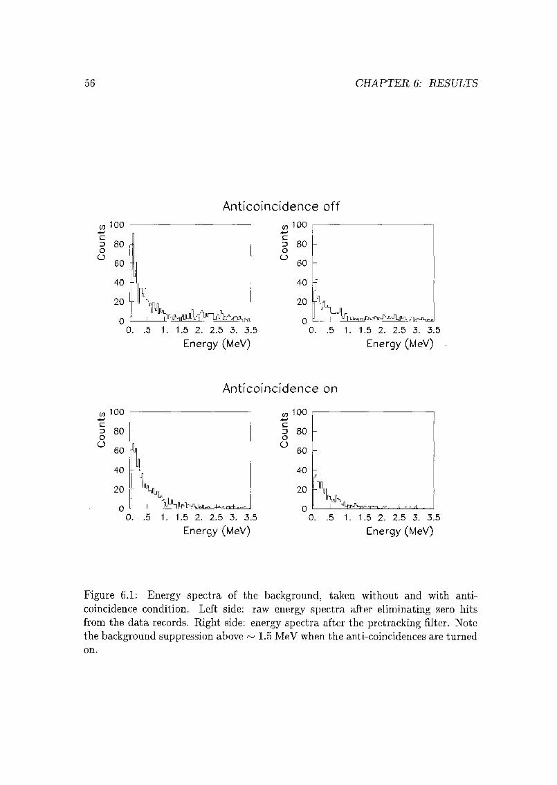
56 CHAPTER 6: RESULTS
Anticoincidence off
100
0. .5 1. 1.5 2. 2.5 3. 3.5
Energy (MeV)
0. .5 1. 1.5 2. 2.5 3. 3.5
Energy (MeV)
Anticoincidence on
1. 1.5 2. 2.5 3. 3.5
Energy (MeV)
0. .5 1. 1.5 2. 2.5 3. 3.5
Energy (MeV)
Figure 6.1: Energy spectra of the background, taken without and with anti¬
coincidence condition. Left side: raw energy spectra after eliminating zero hits
from the data records. Right side: energy spectra after the pretracking filter. Note
the background suppression above ~ 1.5 MeV when the anti-coincidences are turned
on.
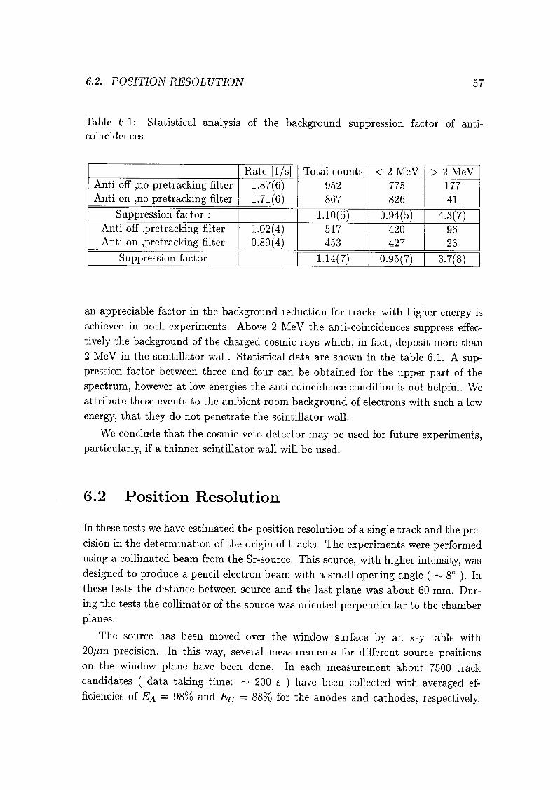
6.2. POSITION RESOLUTION 57
Table 6.1: Statistical analysis of the background suppression factor of anti¬
coincidences
Rate [1/s] Total counts < 2 MeV > 2 MeV
Anti off ,no pretracking filter
Anti on ,no pretracking filter
1.87(6)1.71(6)
952
867
775
826
177
41
Suppression factor : 1.10(5) 0.94(5) 4.3(7)Anti off ,pretracking filter
Anti on ,pretracking filter
1.02(4)0.89(4)
517
453
420
427
96
26
Suppression factor 1.14(7) 0.95(7) 3.7(8)
an appreciable factor in the background reduction for tracks with higher energy is
achieved in both experiments. Above 2 MeV the anti-coincidences suppress effec¬
tively the background of the charged cosmic rays which, in fact, deposit more than
2 MeV in the scintillator wall. Statistical data are shown in the table 6.1. A sup¬
pression factor between three and four can be obtained for the upper part of the
spectrum, however at low energies the anti-coincidence condition is not helpful. We
attribute these events to the ambient room background of electrons with such a low
energy, that they do not penetrate the scintillator wall.
We conclude that the cosmic veto detector may be used for future experiments,
particularly, if a thinner scintillator wall will be used.
6.2 Position Resolution
In these tests we have estimated the position resolution of a single track and the pre¬
cision in the determination of the origin of tracks. The experiments were performed
using a collimated beam from the Sr-source. This source, with higher intensity, was
designed to produce a pencil electron beam with a small opening angle ( ~ 8° ). In
these tests the distance between source and the last plane was about 60 mm. Dur¬
ing the tests the collimator of the source was oriented perpendicular to the chamber
planes.
The source has been moved over the window surface by an x-y table with
20/im precision. In this way, several measurements for different source positionson the window plane have been done. In each measurement about 7500 track
candidates ( data taking time: ~ 200 s ) have been collected with averaged ef¬
ficiencies of Ea — 98% and Ec — 88% for the anodes and cathodes, respectively.
58 CHAPTER 6: RESULTS
m1000
c
g 800
600
400
200
0
es
ZR=0 mm<Z>=0.7mm
°RMS —
1.2 mm
20 -10 0 10 20
Z [mm]
Cathodes
OT1000
c
g 800
600
400
200
0
XR=0 mm<X>= -0.3 mm
°"rms —
1.6 mm
20-10 0 10 20
X [mm!
Figure 6.2: Histograms of track coordinates on the window plane. Left histogram:
vertical coordinate (anodes). Right histogram: horizontal coordinate (cathodes).
Before fitting, the pretracking filter has been used to select the data records. After
the fits about 95% of track candidates have been identified as useful events for the
analysis.
In order to assess a precision in the track extrapolations beyond the body of the
chamber we investigated the distribution of reconstructed positions of the tracks on
the chamber window ( figure 6.2 ). A narrow peak, corresponding to the position
of the source and a low level of background was observed. The two projected his¬
tograms of figure 6.2 can be used to estimate the position resolution for a single
track. It amounts to 1.6 mm for the cathodes ( horizontal coordinate ) and 1.2
mm for the anodes ( vertical coordinate ). In addition, from the centroid of these
histograms we obtain the position (< X >, < Z >) of the source. By comparing
this quantity with an external reference, ( the position Xr, Zr on the x-y table ) we
can find the precision of track extrapolation.
Several measurements have been done, where all the chamber has been scanned
horizontally ( vertically) in steps of 3 mm. Figure 6.3 shows the deviation
( A =< Z > —ZR and A =< X > —Xr for anodes respectively cathodes ) of
the histogram centroids from the nominal position. This deviation is less than 600
/im for both coordinates and shows a periodic structure which has been fitted with
a sinus curve. The period length of the curve ( À ~ 12 mm, see table 6.2 ) shows
that the structure is a result of the discretization in the coordinates of the wires (wire spacing: 4 mm, sampling interval distance: 3 mm ). A residual of the cen¬
troid position has been obtained by subtracting the sinus curve from the centroid
coordinates.
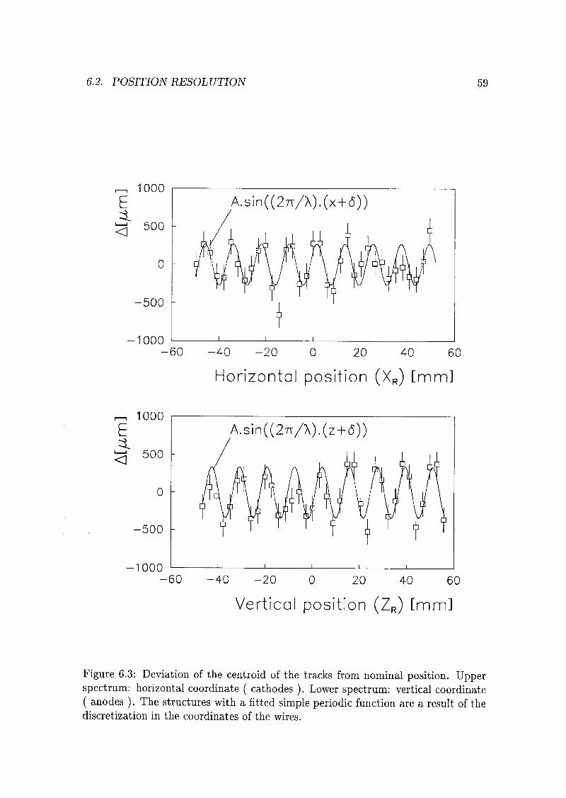
6.2. POSITION RESOLUTION 59
,-,1000
^ 500
0
500
-1000
-60 -40 -20 0 20 40 60
Horizontal position (XR) [mm]
^ 500
-500 -
-1000
-60 -40 -20 0 20 40 60
Vertical position (ZR) [mm]
Figure 6.3: Deviation of the centroid of the tracks from nominal position. Upperspectrum: horizontal coordinate ( cathodes ). Lower spectrum: vertical coordinate
( anodes ). The structures with a fitted simple periodic function are a result of the
discretization in the coordinates of the wires.
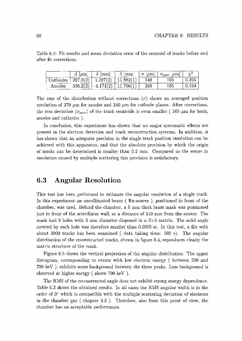
60 CHAPTER 6: RESULTS
Table 6.2: Fit results and mean deviation error of the centroid of tracks before and
after fit corrections.
A [/xm] ö [mm] A [mm] a [/tm] acorr [/im] x2Cathodes 267.9(3) 1.287(2) 11.882(1) 240 165 0.265
Anodes 336.2(2) -1.171(2) 11.706(1) 268 165 0.154
The rms of the distribution without corrections (a) shows an averaged position
resolution of 270 /im for anodes and 240 /im for cathode planes. After corrections,
the rms deviation (<7corr) of the track centroids is even smaller ( 165 p,m for both,
anodes and cathodes ).
In conclusion, this experiment has shown that no major systematic effects are
present in the electron detection and track reconstruction systems. In addition, it
has shown that an adequate precision in the single track position resolution can be
achieved with this apparatus, and that the absolute precision by which the origin
of tracks can be determined is smaller than 0.2 mm. Compared to the errors in
resolution caused by multiple scattering this precision is satisfactory.
6.3 Angular Resolution
This test has been performed to estimate the angular resolution of a single track.
In this experiment an uncollimated beam ( Ru-source ), positioned in front of the
chamber, was used. Behind the chamber, a 5 mm thick brass mask was positioned
just in front of the scintillator wall, at a distance of 110 mm from the source. The
mask had 9 holes with 3 mm diameter disposed in a 3x3 matrix. The solid angle
covered by each hole was therefore smaller than 0.0005 sr. In this test, a file with
about 3000 tracks has been examined ( data taking time: 500 s). The angulardistribution of the reconstructed tracks, shown in figure 6.4, reproduces clearly the
matrix structure of the mask.
Figure 6.5 shows the vertical projection of the angular distribution. The upper
histogram, corresponding to events with low electron energy ( between 250 and
700 keV ), exhibits some background between the three peaks. Less background is
observed at higher energy ( above 700 keV ).
The RMS of the reconstructed angle does not exhibit strong energy dependence.
Table 6.3 shows the obtained results. In all cases the RMS angular width is in the
order of 3° which is compatible with the multiple scattering deviation of electrons
in the chamber gas ( chapter 4.3 ). Therefore, also from this point of view, the
chamber has an acceptable performance.
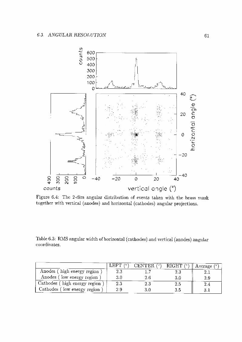
6.3. ANGULAR RESOLUTION 61
: JL
40
cm
20 c
o
"o-M
c
0 oN
4_
oJC
-20
o o o oo o o o
« CO OJ *—
-40
counts
-20 0 20 40
vertîcol angle (°)
-40
Figure 6.4: The 2-dim angular distribution of events taken with the brass mask
together with vertical (anodes) and horizontal (cathodes) angular projections.
Table 6.3: RMS angular width of horizontal (cathodes) and vertical (anodes) angularcoordinates.
LEFT (°) CENTER (°) RIGHT (°) Average (°)Anodes ( high energy region )Anodes ( low energy region )
2.3 1.7 2.3
3.0 2.6 3.0
2.1
2.9
Cathodes ( high energy region )Cathodes ( low energy region )
2.3 2.3 2.5
2.9 3.0 3.5
2.4
3.1
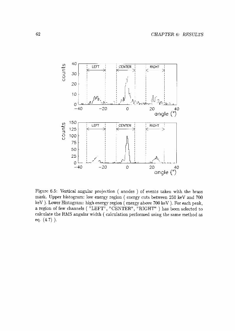
62 CHAPTER 6: RESULTS
CO
c
Z5
OÜ
40
30
20
10
0
co150
c 125D
o 100u
75
50
LEFT
K ^
^^.n
RIGHT
K ^
1F14-J1! 11^ lnü_
-40
25
-40
-20
LEFT
K SH
-20
20
angle (°40
CENTER
K >:
GL.iln — —£L
RIGHT
K >,
^jjl_o -d_
20 40
angle (°)
Figure 6.5: Vertical angular projection ( anodes ) of events taken with the brass
mask. Upper histogram: low energy region ( energy cuts between 250 keV and 700
keV ). Lower Histogram: high energy region ( energy above 700 keV ). For each peak,a region of few channels ( "LEFT", "CENTER", "RIGHT" ) has been selected to
calculate the RMS angular width ( calculation performed using the same method as
eq. (4.7) ).
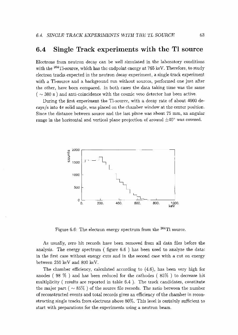
6.4. SINGLE TRACK EXPERIMENTS WITH THE TL SOURCE 63
6.4 Single Track experiments with the Tl source
Electrons from neutron decay can be well simulated in the laboratory conditions
with the 204Tl-source, which has the endpoint energy at 765 keV. Therefore, to study
electron tracks expected in the neutron decay experiment, a single track experiment
with a Tl-source and a background run without sources, performed one just after
the other, have been compared. In both cases the data taking time was the same
( ~ 300 s ) and anti-coincidence with the cosmic veto detector has been active.
During the first experiment the Tl-source, with a decay rate of about 4000 de-
cays/s into 47r solid angle, was placed on the chamber window at the center position.
Since the distance between source and the last plane was about 75 mm, an angular
range in the horizontal and vertical plane projection of around ±40° was covered.
w 2000*->
c
o°
1500
1000
500
0
Figure 6.6: The electron energy spectrum from the 204T1 source.
As usually, zero hit records have been removed from all data files before the
analysis. The energy spectrum ( figure 6.6 ) has been used to analyze the data:
in the first case without energy cuts and in the second case with a cut on energy
between 250 keV and 800 keV.
The chamber efficiency, calculated according to (4.6), has been very high for
anodes ( 98 % ) and has been reduced for the cathodes ( 85% ) to decrease hit
multiplicity ( results are reported in table 6.4 ). The track candidates, constitute
the major part ( ~ 85% ) of the source file records. The ratio between the number
of reconstructed events and total records gives an efficiency of the chamber in recon¬
structing single tracks from electrons above 80%. This level is certainly sufficient to
start with preparations for the experiments using a neutron beam.
200. 400. 600. 800. 1000.keV
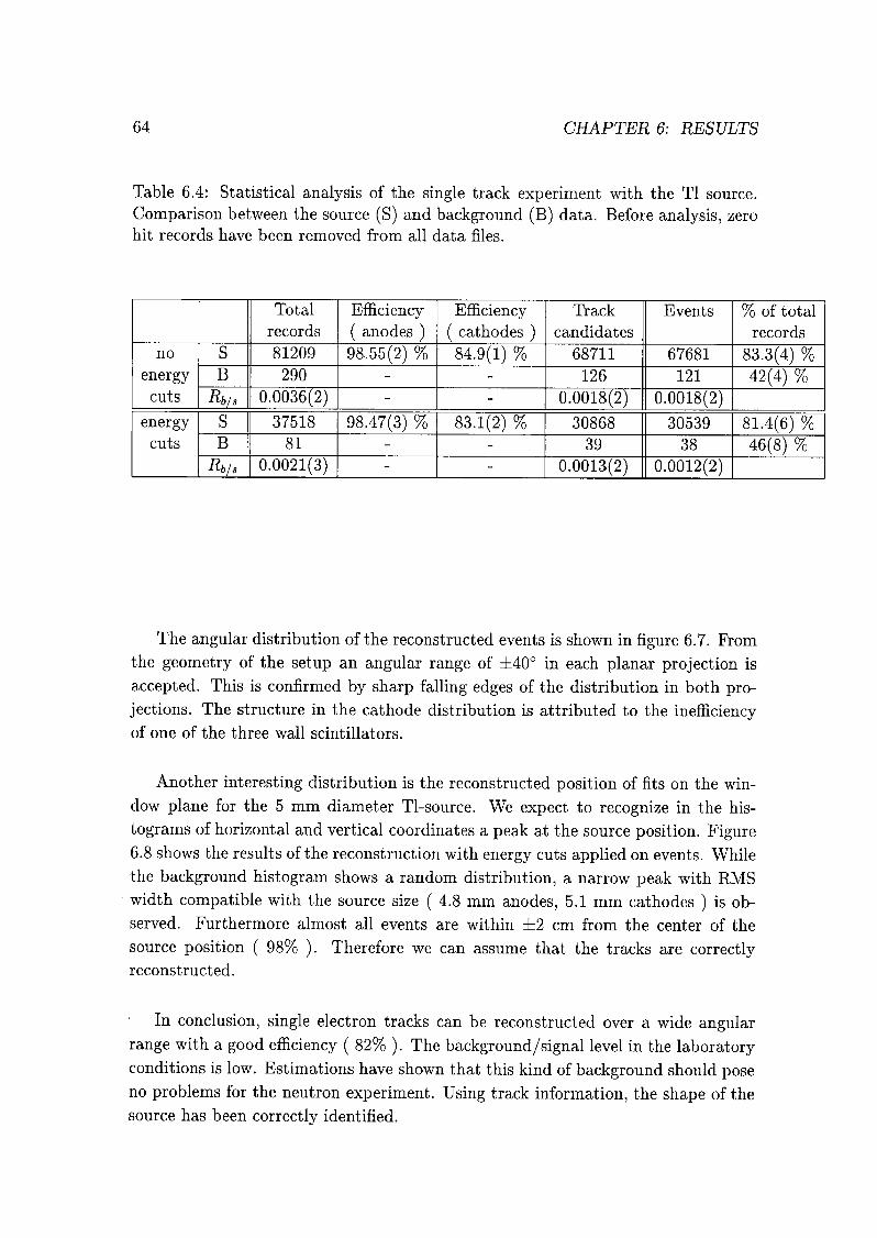
64 CHAPTER 6: RESULTS
Table 6.4: Statistical analysis of the single track experiment with the Tl source.
Comparison between the source (S) and background (B) data. Before analysis, zero
hit records have been removed from all data files.
Total
records
Efficiency
( anodes)Efficiency
( cathodes )
Track
candidates
Events % of total
records
no
energy
cuts
S 81209 98.55(2) % 84.9(1) % 68711 67681 83.3(4) %B 290 - - 126 121 42(4) %
Rb/s 0.0036(2) - - 0.0018(2) 0.0018(2)
energy
cuts
S 37518 98.47(3) % 83.1(2) % 30868 30539 81.4(6) %B 81 - - 39 38 46(8) %
Rb/s 0.0021(3) - - 0.0013(2) 0.0012(2)
The angular distribution of the reconstructed events is shown in figure 6.7. From
the geometry of the setup an angular range of ±40° in each planar projection is
accepted. This is confirmed by sharp falling edges of the distribution in both pro¬
jections. The structure in the cathode distribution is attributed to the inefficiencyof one of the three wall scintillators.
Another interesting distribution is the reconstructed position of fits on the win¬
dow plane for the 5 mm diameter Tl-source. We expect to recognize in the his¬
tograms of horizontal and vertical coordinates a peak at the source position. Figure6.8 shows the results of the reconstruction with energy cuts applied on events. While
the background histogram shows a random distribution, a narrow peak with RMS
width compatible with the source size ( 4.8 mm anodes, 5.1 mm cathodes ) is ob¬
served. Furthermore almost all events are within ±2 cm from the center of the
source position ( 98% ). Therefore we can assume that the tracks are correctlyreconstructed.
In conclusion, single electron tracks can be reconstructed over a wide angular
range with a good efficiency ( 82% ). The background/signal level in the laboratoryconditions is low. Estimations have shown that this kind of background should pose
no problems for the neutron experiment. Using track information, the shape of the
source has been correctly identified.
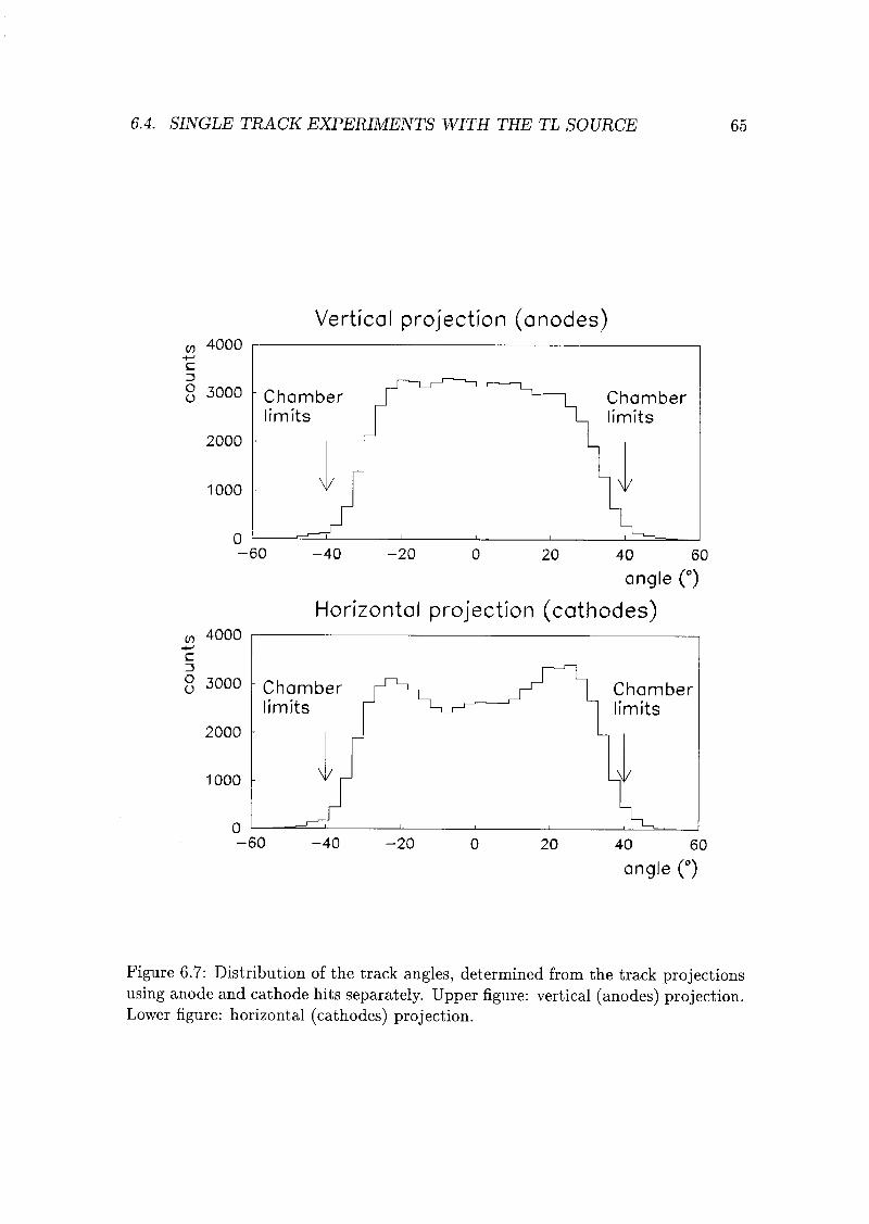
6.4. SINGLE TRACK EXPERIMENTS WITH THE TL SOURCE 65
Vertical projection (anodes)OT 4000
c
g 3000
2000
1000
Chamber
limits
V
Chamber
limits
V
-60 -40 -20 20 40 60
angle (°)
Horizontal projection (cathodes)m 4000
c
g 3000
2000
1000
Chamber
limits
V J
Chamber
limits
\|/
o
-60 -40 -20 20 40 60
angle (°)
Figure 6.7: Distribution of the track angles, determined from the track projections
using anode and cathode hits separately. Upper figure: vertical (anodes) projection.Lower figure: horizontal (cathodes) projection.
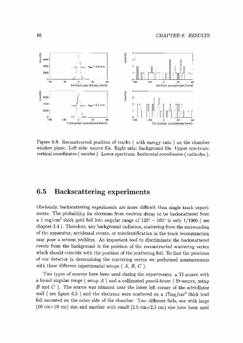
66 CHAPTER 6: RESULTS
V,
c 1§ 6000 1
O L
4000 —>( ^ cr^js = 4.8 mm
2000 / V
w
c
O6000
o
4000
2000
0
-30 0 30 60
Vertical coordinate (mm)
.
J
f\^ iJrus = 5.1 mm
-30 0 30 60
Horizontal coordinate [mm]
4 i
3 -
:L nhnn il L
0
-60
-30 0 30 60
Vertical coordinate [mm]
-30 o 30 60
Horizontal coordinate [mm]
Figure 6.8: Reconstructed position of tracks ( with energy cuts ) on the chamber
window plane. Left side: source file. Right side: background file. Upper spectrum:vertical coordinates ( anodes ). Lower spectrum: horizontal coordinates ( cathodes ).
6.5 Backscattering experiments
Obviously, backscattering experiments are more difficult than single track experi¬ments. The probability for electrons from neutron decay to be backscattered from
a 1 mg/cm2 thick gold foil into angular range of 120° — 160° is only 1/1000 ( see
chapter 3.4 ). Therefore, any background radiation, scattering from the surroundingof the apparatus, accidental events, or misidentification in the track reconstruction
may pose a serious problem. An important tool to discriminate the backscattered
events from the background is the position of the reconstructed scattering vertex
which should coincide with the position of the scattering foil. To find the precisionof our detector in determining the scattering vertex we performed measurements
with three different experimental setups ( A, B, C ).
Two types of sources have been used during the experiments: a Tl source with
a broad angular range ( setup A ) and a collimated pencil-beam ( Sr-source, setupB and C ). The source was situated near the lower left corner of the scintillator
wall ( see figure 6.9 ) and the electrons were scattered on a 17mg/cm2 thick lead
foil mounted on the other side of the chamber. Two different foils, one with large
(10 cmxlO cm) size and another with small (2.5 cmx2.5 cm) size have been used
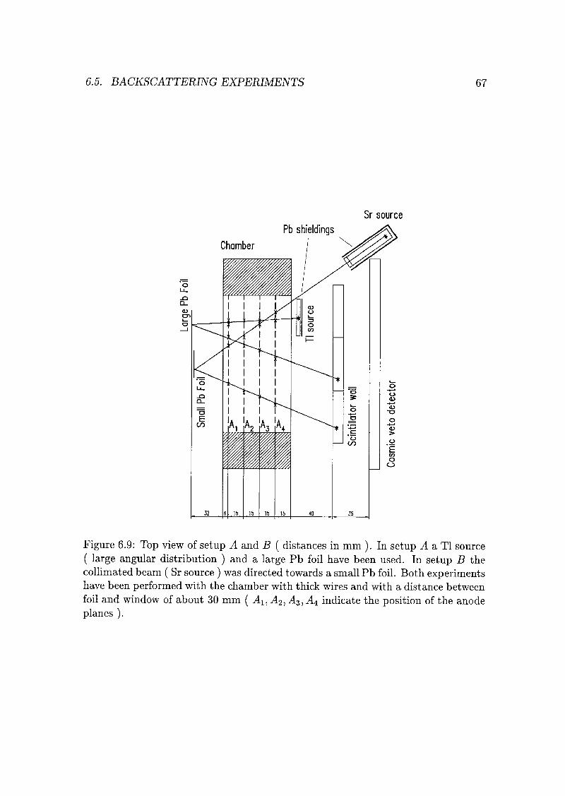
6.5. BACKSCATTERING EXPERIMENTS 67
Sr source
Pb shieldings
Chamber
Figure 6.9: Top view of setup A and B ( distances in mm ). In setup A a Tl source
( large angular distribution ) and a large Pb foil have been used. In setup B the
collimated beam ( Sr source ) was directed towards a small Pb foil. Both experimentshave been performed with the chamber with thick wires and with a distance between
foil and window of about 30 mm ( Ai,A2,As,A4 indicate the position of the anode
planes ).
68 CHAPTER 6: RESULTS
for setup A, respectively B and C. The background has been measured by removing
the scattering foil. To study the electron scattering from the chamber wires tests
have been performed with two different chambers, with 50/xm diameter Ni-Cr and
20 /im diameter W wires ( setup A and B ), and with 25/im diameter Ni-Cr and
10 p.m. diameter W wires ( setup C ), respectively. Table 6.5 reports the principal
characteristics of these three setups.
Table 6.5: Parameters of the three different experimental setups.
Setup Wires Source Collimator
diameter
Foil
size
Foil
thickness
Foil-chamber
distance
A Thick Tl uncollimated 10x10 cm 17mg/cm2 ~ 30 mm
B Thick Sr 1 mm 2.5x2.5 cm 17mg/cm2 ~ 30 mm
C Thin Sr 0.5 mm 2.5x2.5 cm 17mg/cm2 ~ 22 mm
In all experiments the data collection time was about 500 s. For the analysis,
zero hit records have been removed and data with an energy between 250 and 800
keV has been selected ( energy range of neutron decay experiment ).
Both projections are required to find out the position in space of scattering ver¬
tices, Therefore, for this kind of analysis, we selected events having angular aperture
of the two tracks of more than 15° in both coordinates.
After filters, the two-track reconstruction efficiency of anodes E2(A) = Na/Nt
( Nt'. total of selected records, Na' records where a two-track reconstruction
on anodes has been done ) and the backscattering event reconstruction efficiency
E2 = NB/NT ( Nt as before, NB: records where the two-track reconstruction on
anodes and cathodes has been done ) have been measured.
Table 6.6 reports the raw data ("Foil-in" ) and the results after background sub¬
traction ("Foil-in"- "Foil-out"). The low efficiency of the raw data is a consequence
of the high level of background. After background subtraction, much better results
are obtained ( E2 > 50% and E2(A) > 68% ) for all three setups. The results of
setup A are substantially worser than in the other two setups. We attribute this to
different geometrical conditions: in setup A the foil size was almost matching the size
of the detector active area, therefore a considerable amount of electrons traversed
the chamber near the edges and were lost in the walls of the wire chamber.
If we average the results of setup B and C, which pose no problems with chamber
edges, we obtain an anode efficiency E2(A) ~ 85% and a total backscattering event
reconstruction efficiency E2 ~ 70% ( average of the two measurements ). Further
refinement should improve this result.
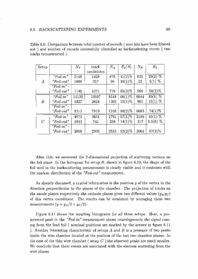
6.5. BACKSCATTERING EXPERIMENTS 69
Table 6.6: Comparison between total number of records ( zero hits have been filtered
out ) and number of records successfully identified as backscattering events ( two
tracks reconstructed ).
Setup NT track
candidates
NA E2(A) NB E2
A
"Foil-in"
"Foil-out"
2148
1008
1428
357
876
98
41(2)%10(1)%
621
53
29(2) %
5(1) %"Foil-in" -
"Foil-out" 1140 1071 778 68(3)% 568 50(2)%
B
"Foil-in"
"Foil-out"
14139
5927
10597
2624
8548
1302
60(1)%22(1)%
6944
861
49(1) %
15(1) %"Foil-in"-
"Foil-out" 8212 7973 7246 88(2)% 6083 74(1)%
C
"Foil-in"
"Foil-out"
4872
1813
3651
745
2791
258
57(1)%14(1)%
2180
117
45(1) %
6.5(6) %"Foil-in" -
"Foil-out" 3059 2906 2533 83(2)% 2063 67(2)%
After this, we recovered the 2-dimensional projection of scattering vertices on
the foil plane. In the histogram for setup B, shown in figure 6.10, the shape of the
foil used in the backscattering measurement is clearly visible and it contrasts with
the random distribution of the "Foil-out" measurement.
As already discussed, a crucial information is the position y of the vertex in the
direction perpendicular to the planes of the chamber. The projection of tracks on
the anode planes respectively the cathode planes gives two different values (yA,Vc)of this vertex coordinate. The results can be combined by averaging these two
measurements (y — ya/"2 + yc/2).
Figure 6.11 shows the resulting histograms for all three setups. Here, a pro¬
nounced peak in the "Foil-in" measurement shows unambiguously the signal com¬
ing from the lead foil ( nominal positions are marked by the arrows in figure 6.11
). Another interesting characteristic of setups A and B is a presence of two peaks
inside the wire chamber located at the position of the last two chamber planes. In
the case of the thin wire chamber ( setup C ) the observed peaks are much smaller.
We conclude that these events are associated with the electron scattering from the
wire planes.
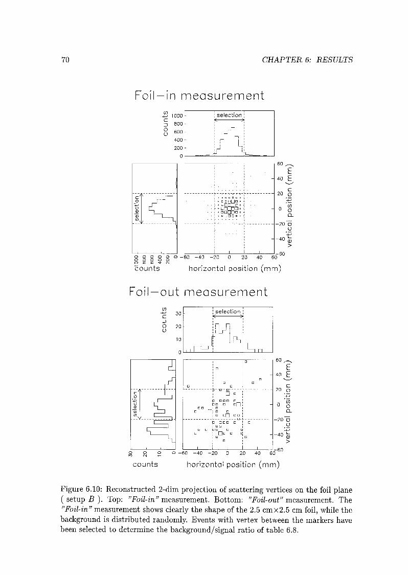
70 CHAPTER 6: RESULTS
Foîl —în measurement
-
i—,.,_,—,_ ,_
c ,= o n
o
«1
i"nnn-
! • a GOTta "
!• DTDa »
• i •nnGDD °
[ . Q D D a
-
CO/ ri L._- u
i i i i
60^^
E40 E
20 O
0 3
-20 D(J
-40
o o o o o o -60 -40o o o o oO (O to ^ c\|
-20 20 40 60-60
counts horizontal position (mm)
Foil —out measurement
^
~s
b--n--o
ID a
tp nan n
pa d DfJDD rji D
3 | D Q
i d n[~J n
b ODD D
i a d
a a d
Da d q
60^-^
E40 E
r2U o
-*-'
mU O
Cl
-20 "du
-h->
-40(D
>
o q o o -60 -40 -20 0 20 40 60fO CN y—
-60
counts horizontal position (mm)
Figure 6.10: Reconstructed 2-dim projection of scattering vertices on the foil plane
(setups). Top: "Foil-in" measurement. Bottom: "Foil-out" measurement. The
"Foil-in" measurement shows clearly the shape of the 2.5 cmx2.5 cm foil, while the
background is distributed randomly. Events with vertex between the markers have
been selected to determine the background/signal ratio of table 6.8.
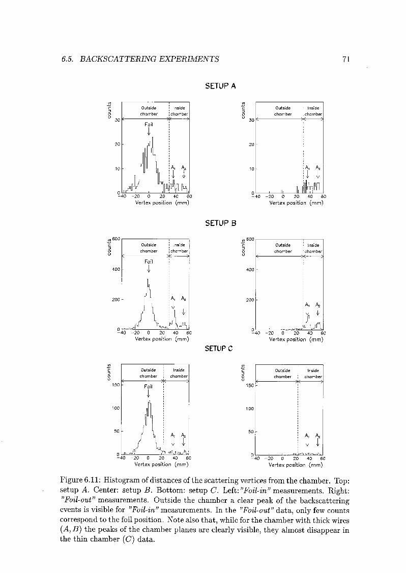
6.5. BACKSCATTERING EXPERIMENTS 71
SETUP A
-40 -20 0 20 40 60
Vertex position (mm)
30
10
Outside
chamber
Inside
,chamber
-X ^
i A, A2
ta-40 -20 0 20 40 60
Vertex position (mm)
,600
200
Outside
chamber
Foil
i Inside
I chamber
A, A2
-40 -20 0 20 40 60
Vertex position (mm)
SETUP B
SETUP C
400
200
Outside
chamber
-X-
Insfde
chamber
n
-40 -20 0 20 40 60
Vertex position (mm)
150
Outside i Inside
chamber,
chamber
Nn-rV-40 -20 0 20 40 60
Vertex position (mm)
150
50
Outside
chamber
Inside
chamber
* N
niir^tfVJUr-^na,
-40 -20 0 20 40 60
Vertex position (mm)
Figure 6.11: Histogram of distances of the scattering vertices from the chamber. Top:setup A Center: setup B. Bottom: setup C. Left: "Foil-in" measurements. Right:"Foil-out" measurements. Outside the chamber a clear peak of the backscatteringevents is visible for "Foil-in" measurements. In the "Foil-out" data, only few counts
correspond to the foil position. Note also that, while for the chamber with thick wires
(A, B) the peaks of the chamber planes are clearly visible, they almost disappear in
the thin chamber (C) data.
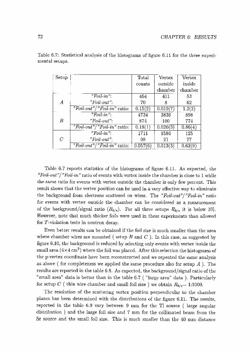
72 CHAPTER 6: RESULTS
Table 6.7: Statistical analysis of the histograms of figure 6.11 for the three experi¬mental setups.
Setup Total
counts
Vertex
outside
chamber
Vertex
inside
chamber
A
"Foil-in":
"Foil-out":
464
70
411
8
53
62
"Foil-out"/"Foil-in" ratio: 0.15(2) 0.019(7) 1.2(2)
B
"Foil-in":
"Foil-out":
4734
874
3836
100
898
774
"Foil-out"/"Foil-in" ratio: 0.18(1) 0.026(3) 0.86(4)
C
"Foil-in":
"Foil-out":
1711
98
1586
21
125
77
"Foil-out"/"Foil-in" ratio: 0.057(6) 0.013(3) 0.62(9)
Table 6.7 reports statistics of the histograms of figure 6.11. As expected, the
"Foil-out"/ "Foil-in" ratio of events with vertex inside the chamber is close to 1 while
the same ratio for events with vertex outside the chamber is only few percent. This
result shows that the vertex position can be used in a very effective way to eliminate
the background from electrons scattered on wires. The "Foil-out"j"Foil-in" ratio
for events with vertex outside the chamber can be considered as a measurement
of the background/signal ratio (Rb/S)- For all three setups Rb/S it is below 3%.
However, note that much thicker foils were used in these experiments than allowed
for T-violation tests in neutron decay.
Even better results can be obtained if the foil size is much smaller than the area
where chamber wires are mounted ( setup B and C ). In this case, as suggested by
figure 6.10, the background is reduced by selecting only events with vertex inside the
small area (4x4 cm2) where the foil was placed. After this selection the histograms of
the ^/-vertex coordinate have been reconstructed and we repeated the same analysisas above ( for completeness we applied the same procedure also for setup A ). The
results are reported in the table 6.8. As expected, the background/signal ratio of the
"small area" data is better than in the table 6.7 ( "large area" data ). Particularlyfor setup C ( thin wire chamber and small foil size ) we obtain Rb/S= 1:1000.
The resolution of the scattering vertex position perpendicular to the chamber
planes has been determined with the distributions of the figure 6.11. The results,
reported in the table 6.9 vary between 9 mm for the Tl source ( large angulardistribution ) and the large foil size and 7 mm for the collimated beam from the
Sr source and the small foil size. This is much smaller than the 40 mm distance
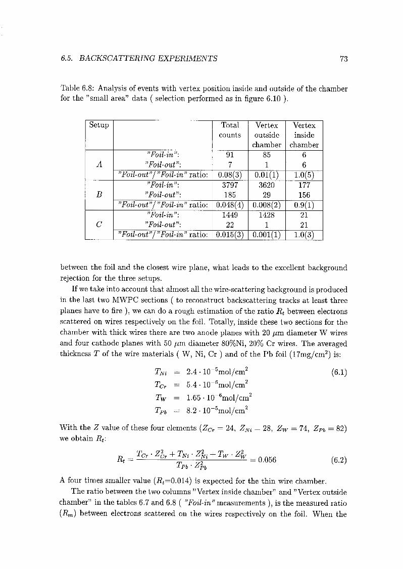
6.5. BACKSCATTERING EXPERIMENTS 73
Table 6.8: Analysis of events with vertex position inside and outside of the chamber
for the "small area" data ( selection performed as in figure 6.10 ).
Setup Total
counts
Vertex
outside
chamber
Vertex
inside
chamber
A
"Foil-in":
"Foil-out":
91
7
85
1
6
6
"Foil-out"/"Foil-in" ratio: 0.08(3) 0.01(1) 1.0(5)
B
"Foil-in":
"Foil-out":
3797
185
3620
29
177
156
"Foil-out"1'"Foil-in" ratio: 0.048(4) 0.008(2) 0.9(1)
C
"Foil-in":
"Foil-out":
1449
22
1428
1
21
21
"Foil-out"/"Foil-in" ratio: 0.015(3) 0.001(1) 1.0(3)
between the foil and the closest wire plane, what leads to the excellent background
rejection for the three setups.
If we take into account that almost all the wire-scattering background is producedin the last two MWPC sections ( to reconstruct backscattering tracks at least three
planes have to fire ), we can do a rough estimation of the ratio Rt between electrons
scattered on wires respectively on the foil. Totally, inside these two sections for the
chamber with thick wires there are two anode planes with 20 /im diameter W wires
and four cathode planes with 50 fim. diameter 80%Ni, 20% Cr wires. The averagedthickness T of the wire materials ( W, Ni, Cr ) and of the Pb foil (17mg/cm2) is:
Tm = 2.4 • 10-5mol/cm2 (6.1)
TCr = 5.4 • 10"6mol/cm2
Tw = 1.65 • 10~6mol/cm2
TPb = 8.2 10-5mol/cm2
With the Z value of these four elements (ZCr = 24, ZNi = 28, Zw = 74, ZPb = 82)we obtain Rt:
Rt =TCr-ZCr + TNi-ZJi+TW.Z2w = o o56 ^ 2)
J-Pb zPb
A four times smaller value (Rt=0.01A) is expected for the thin wire chamber.
The ratio between the two columns "Vertex inside chamber" and "Vertex outside
chamber" in the tables 6.7 and 6.8 ( "Foil-in" measurements ), is the measured ratio
(Rm) between electrons scattered on the wires respectively on the foil. When the
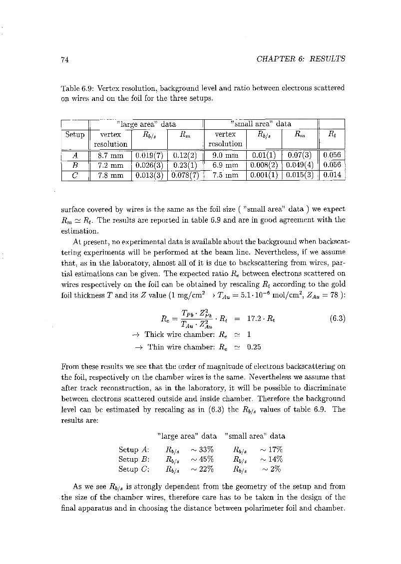
74 CHAPTER 6: RESULTS
Table 6.9: Vertex resolution, background level and ratio between electrons scattered
on wires and on the foil for the three setups.
"large area" data "small area" data
Setup vertex
resolution
Rb/s *Wn vertex
resolution
Rb/s ^m Rt
A 8.7 mm 0.019(7) 0.12(2) 9.0 mm 0.01(1) 0.07(3) 0.056
B 7.2 mm 0.026(3) 0.23(1) 6.9 mm 0.008(2) 0.049(4) 0.056
C 7.8 mm 0.013(3) 0.078(7) 7.5 mm 0.001(1) 0.015(3) 0.014
surface covered by wires is the same as the foil size ( "small area" data ) we expect
Rm ~ Rt. The results are reported in table 6.9 and are in good agreement with the
estimation.
At present, no experimental data is available about the background when backscat¬
tering experiments will be performed at the beam line. Nevertheless, if we assume
that, as in the laboratory, almost all of it is due to backscattering from wires, par¬
tial estimations can be given. The expected ratio Re between electrons scattered on
wires respectively on the foil can be obtained by rescaling Rt according to the gold
foil thickness T and its Z value (1 mg/cm2 -> TAu = 5.1 • 10-6 mol/cm2, ZAu = 78 ):
= 17.2-A* (6.3)
~ 1
~ 0.25
From these results we see that the order of magnitude of electrons backscattering on
the foil, respectively on the chamber wires is the same. Nevertheless we assume that
after track reconstruction, as in the laboratory, it will be possible to discriminate
between electrons scattered outside and inside chamber. Therefore the background
level can be estimated by rescaling as in (6.3) the Rb/S values of table 6.9. The
results are:
"large area" data "small area" data
Setup A: Rb/s ~ 33% Rb/s ~ 17%
Setup B: Rb/s ~ 45% Rb/s ~ 14%
Setup C: RbJs ~ 22% Rb/s ~ 2%
As we see Rb/S is strongly dependent from the geometry of the setup and from
the size of the chamber wires, therefore care has to be taken in the design of the
final apparatus and in choosing the distance between Polarimeter foil and chamber.
P _
TPb ZPb
J-Au "
^Au
—> Thick wire chamber: Re
—> Thin wire chamber: Re

6.5. BACKSCATTERING EXPERIMENTS 75
In addition the calculations reported here are imprecise, since at the beam line the
impact of other background types is unknown.
In conclusion, laboratory experiments have shown that it is possible to detect the
electrons backscattered from Polarimeter foils with a good efficiency. A good level
of signal to background has been measured. Particularly, the background could be
reduced by using the chamber with thin wires and by applying proper geometricalselection ( "small area" ) of the data. This analysis has demonstrated that detec¬
tion of a track vertex is a powerful tool in discrimination against the backgroundradiation. Finally the ratio between background and signal for the neutron decay
experiment will be most probably determined by local radiation around the neutron
beam guide and out of beam scattered neutrons.

CHAPTER 6: RESULTS
Chapter 7
Summary and Conclusions
With this work an attempt to measure for the first time the R correlation in neutron
decay has been started. In the following we present a summary of the obtained
results:
• The neutrons, produced in the spallation source SINQ, will be longitudinally
polarized with the aid of magnetic supermirrors. RF-spin flippers and analyz¬
ers will be used to change, respectively to measure the longitudinal neutron
polarization, which is expected to be high (~ 95%). A MWPC gas trackingdetector with cylindrical shape ( length=l m, diameter=30 cm ) has been
proposed to perform the experiment. Mott scattering from a thin gold foil
will be used to measure the electron polarization. The foil, surrounding the
apparatus, will have a thickness of ~ 1 mg/cm2 ( limitation due to multiple
scattering effects ). Electrons with energy between 250 keV and 780 keV will
be selected for the experiment. The averaged analyzing power of the apparatus
without respectively with inclusion of multiple scattering effects is < S >—-
0.3, respectively < S >=-0.2. The data taking time necessary to measure R
with a precision of 0.01, for a total neutron flux of 2 • 109/s, is in the order of
weeks.
• A small-size ( 20x20 cm2 ) planar chamber prototype, consisting of 4 MWPC
sections, has been developed to test the feasibility of the experiment. To re¬
construct the trajectory of particles four anode planes ( vertical coordinate )and four cathode planes ( horizontal coordinate ) have been read out. On
each plane, the wires have been placed every 4 mm. Scintillators have been
used to measure the energy of particles and provide a fast trigger signal. He-
lium/methylal gas mixtures have been investigated as chamber filling gases.
For these gas mixtures deviations of the electron trajectory because of mul¬
tiple scattering effects are acceptable. With these gases a high efficiency per
MWPC plane ( > 98% anodes, > 86% cathodes ) has been obtained. Opti¬mizations have been done to reduce hit multiplicity ( the number of neighbor
77
78 CHAPTER 7: SUMMARY AND CONCLUSIONS
wires firing on one plane after the passage of particles ) while preserving a
high detection efficiency. A minimal hit multiplicity is important for track
reconstruction. Good results have been obtained over a wide angular range.
• The detector response was tested using three /3-decay sources ( 204T1, 90Sr
and 106Ru ). The energy endpoint of the three sources is 765 keV for Tl
( similar as the /3-decay spectrum of neutrons ), 2.28 MeV for Sr and 3.7 MeV
for Ru. The precision in track reconstruction has been measured in one-track
experiments with a collimated beam ( Sr source ). The position resolution of a
single track was better than 2 mm. The angular resolution of tracks, measured
with the aid of a brass mask, was around 3°. Experiments with the Tl source
and experiments without sources have been compared to estimate the amount
of one-track events produced by ambient background. The background/signalratio measured in the laboratory was very low (~ 1 : 1000). A high one-track
reconstruction efficiency (~ 80%) has been measured with the Tl source ( wide
angular range ). The same efficiency is expected for electrons from neutron
decay.
• To perform backscattering experiments 17 mg/cm2 thick Pb foils have been
used. Measurements have been done with three different setups. In the first
one a thick wire chamber ( 50 ^m diameter cathodes and 20 //m diameter
anodes ), a Tl source ( wide angular range ) and a large scattering foil have
been used. In the second one the chamber was the same, but a collimated
beam ( Sr source ) and a small size foil have been used. In the last ex¬
periment we used a chamber with two times thinner wires. In each setup
the background ( like, for example, two-track events produced by electrons
scattering on chamber material ) has been measured with foil removed, but
with the source left inserted. For all three setups complete tracks ( anodes
and cathodes ) of backscattering electrons have been reconstructed with an
efficiency above 50%. The most important results have been obtained us¬
ing the vertex position information. Using the scattering vertex coordinate
perpendicular to chamber planes, the foil position has been extracted with a
precision of ~ 7 mm and it has been shown that most of the background in
laboratory conditions originates from electrons scattering on chamber wires.
This foil position resolution is much smaller than the distance between foil
and first wire plane ( ~ 40 mm ) and has been used to obtain an excellent
background/signal ratio ( 1:100 for the thick wire chamber and 1:1000 for
the thin wire chamber ). The ratio between electrons scattered on wires and
electrons scattered on the foil has been estimated ( 0.056 thick wire chamber,0.014 thin wire chamber ) by comparing the amount of materials inside and
outside the chamber. A good agreement with the experimental results has
CHAPTER 7: SUMMARY AND CONCLUSIONS 79
been found. No data is available about the background when backscattering
experiments will be performed at the cold neutron beam line. However partial
estimations have been done assuming that almost all background will be given
by electrons scattering on wires. For the neutron experiment, where a thin
(1 mg/cm2) scattering gold foil will be used, the amounts of electrons scatter¬
ing on wires respectively on the foil will be on the same order of magnitude.
If, as in the laboratory, vertex information will be used, it will be possible to
remove from the data the major part of this background.
These are promising results, therefore we propose to use this detector prototype
for first measurements at the beam line. Nevertheless, contrary to the laboratoryconditions were all the sources used were point sources, at the beam line the neutrons
will have a large spatial distribution. For each backscattering electron event, this
introduces difficulties in distinguishing between the primary decay track and the
track of the electron after scattering. To avoid this, additional information could
be obtained with a second MWPC detector. The two detectors could be placed left
and right to the beam line. In this way, while the tracks of electrons coming from
neutron decay would be detected by only one detector, the tracks of electrons after
scattering would be detected by both chambers. The second MWPC detector would
be also very useful to suppress the background.The conclusion of this work is that, under assumption of an adequate control
of the background conditions around the neutron beam, a measurement of the R
parameter in neutron decay at the spallation source SINQ at PSI is feasible. This
would be the first such determination and a stringent test of time reversal symmetry
in weak interactions.

80 CHAPTER 7: SUMMARY AND CONCLUSIONS

Bibliography
[1] T.D. Lee, C.N. Yang, Phys. Rev. 104(1956)254.
[2] CS. Wu et al, Phys. Rev. 105(1957)1413.
[3] J.H. Christenson et al., Phys. Rev. Lett. 13(1964)138.
[4] G. Arnison et al., Phys. Lett. 122B(1983)103;M. Banner et al., Phys. Lett. 122B(1983)476.
[5] G. Arnison et al., Phys. Lett. 126B(1983)398;P. Bagnaiaet al., Phys. Lett. 129B(1983)130.
[6] S.L. Glashow, Nucl. Phys. 22(1961)579;S. Weinberg, Phys. Rev. Lett. 19(1967)1264;A. Salam, inEieimentary Particle Theory
ed. N. Svartholm, (Almqvist and Wiksells 1969), p.367.
[7] Review of Particle Physics, Phys. Rev. D54(1996).
[8] S. Weinberg, Phys. Rev. Lett. 42(1979)850.
[9] E. Blanke et al., Phys. Rev. Lett. 51(1983)355.
[10] See for ex. LS. Altarev et al., Phys. Lett. B276(1992)242.
[11] D. Cho et al, Phys. Rev. Lett. 63(1989)2559.
[12] J. Deutsch, P. Quin, Precision tests of the standard electroweak model
ed. P. Langacker, World Scientific, Singapore 1995, p. 706.
[13] J.D. Jackson, S.B. Treiman, H.W. Wild, Phys. Rev. 106(1957)517.
[14] P. Herczeg Fundamental Symmetries in Nuclei and Particles
ed. H. Henrikson and P.Vogel, World Scientific, Singapore 1989, p. 46.
[15] M.T. Burgy et al., Phys. Rev. 120(1960)829.
[16] B.G. Erozolimskii, JETP Lett. 20(1974)345.
81
82 BIBLIOGRAPHY
[17] R. I. Steinberg, et al. Phys. Rev. D13(1976)2469.
[18] A.L. Hallin et al., Phys. Rev. Lett. 52(1984)337.
[19] M.B Schneider et al., Phys. Rev. Lett. 51(1983)1239.
[20] J. Sromicki et al., Phys. Rev. C 53(1996)932.
[21] J. Sromicki, Habilitation ETH Zürich 1994.
[22] M.Morita Beta decay and Muon decay.
[23] B.G. Erozolimskii et al., Phys. Lett. B 263(1991)33.
[24] K. Schreckenbach et al., Phys. Lett. B 349(1995)427.
[25] H. Abele et al., Phys. Lett. B 407(1997)212.
[26] R. G. Sachs in The Physics of Time Reversal
University of Chicago Press, 1985, Chapter 5.
[27] J.D. Jackson, S.B. Treiman, H.W. Wild, Nucl. Phys. 4(1957)206.
[28] N. Sherman, Phys. Rev. 103 (1956)1601.
[29] S. Hanna, in Symposium on Polarization Phenomena in Nuclear
Physics, Karlsruhe, 1965.
[30] G.S. Bauer and J. F. Crawford, The Spallation Neutron Source SINQ PSI
Report, 1994.
[31] Courtesy of PSI, SINQ technical staff. The spectrum has been recorded at
december 1996 by time of flight measurement at the SINQ neutron guide
1RNR14.
[32] F. Mezei Communications on physics 1 (1976) 81.
[33] F. Mezei Communications on physics 2 (1977) 41.
[34] J.B. Hayter and H. A. Mook, J.Appl. Cryst. 22 (1989) 35.
[35] P. Boni et al., IAEA Proc. Neutron Beam Research 1997 Portugal.
[36] J. Sromicki, Personal Communication.
[37] A. P. Serebrov et al., Nucl. Instr. and Meth. A 357(1995)503.
[38] N.F. Mott and H.S.Massey., The theory of atomic collisions Clarendon
Press Oxford 1965.
BIBLIOGRAPHY 83
[39} T.J. Gay and F. B. Dunning, Rev.Sci.Instrum 63 (1992) 1635.
[40] D. Conti et al., Helv. Phys. C 53 (1996)932.
[41] V. Hnizdo Nucl. Instr. and Meth. 109 503(1973).
[42] G. Charpak et al. Nucl. Instr. and Meth. 62 235(1968).
[43] G. Charpak Evolution of automatic spark chambers
Ann. Rev. Nucl. Sei. 20 195(1970).
[44] F. Sauli CERN Yellow Report 77-09, 1977.
[45] J. Vavra, SLAC PUB-7627 August 1997.
[46] G. Fischer and J.Plch Nucl. Instr. and Meth. 72 515(1972).
[47] TANDEM A data aquisition system ( PSI Publication ).
[48] M.J. Berger and S.B.Seltzer Tables ofenergy losses and ranges for electrons
and positrons NASA SP-3012, 1964.
[49] W.R. Leo, Techniques for Nuclear and Particle Physics Experiments
Springer Verlag 1987, p. 122.
[50] W.T. Scott, Rev. Mod. Phys. 35 (1963) 231.
[51] G. Charpak et al. Nucl. Instr. and Meth. 80 13(1970).
[52] A. Breskin et al. Nucl. Instr. and Meth. 143 29(1977).
[53] Review of Particle Properties, Phys. Rev. D45III.5(1992).
[54] CERN Program Library, Long Writeup Q121.
[55] G. Charpak et al. Nucl. Instr. and Meth. 88 149(1970).

84 BIBLIOGRAPHY

List of Figures
3.1 Principle of the experiment 14
3.2 Schematic view of the cylindrical experimental setup 14
3.3 Decay event 15
3.4 The energy spectrum W(E) of decay electrons 17
3.5 The elastic scattering cross section and the analyzing power of 79Au.
17
3.6 The neutron flux in the supermirror guide 1RNR14 21
3.7 Plan of the beamline 22
3.8 The gold foil thickness for which Seff/S = 2/3 24
3.9 Polarimeter constraint 26
4.1 Schematic layout of the setup 30
4.2 Photograph of the experimental apparatus 31
4.3 The multilayer structure of the chamber 33
4.4 Anode and cathode pulses 35
4.5 The anode and cathode circuits 35
4.6 Efficiency of the anodes for 4 different gas mixtures 38
4.7 The anode hit multiplicity 39
4.8 Distribution of the cathode hit and cathode plane multiplicity ....41
4.9 Example of the chamber setup procedure ( cathodes ) 43
4.10 The energy loss spectrum of Ru/3-particles 44
4.11 Sr and Tl /3-spectra 45
4.12 Energy calibration curve 46
5.1 Spectrum of the collimated beam ( Sr source ) before and after filter¬
ing out zero hit records 48
5.2 Example of a single track fit ( anodes ) 50
5.3 Examples of double track reconstructions 52
5.4 Hit multiplicity of anode and cathode planes as a function of the
incidence angle of tracks 53
85

86 LIST OF FIGURES
6.1 Energy spectra of the background 56
6.2 Histograms of track coordinates on the window plane 58
6.3 Deviation of the centroid of the tracks from nominal position 59
6.4 The 2-dim angular distribution of events taken with the brass mask.
61
6.5 Vertical angular projection of events taken with the brass mask....
62
6.6 The electron energy spectrum from the 204T1 source 63
6.7 Distribution of the track angles ( Tl source ) 65
6.8 Reconstructed position of tracks on the chamber window plane ....66
6.9 Top view of setup A and B 67
6.10 Reconstructed 2-dim projection of scattering vertices 70
6.11 Histogram of distances of the scattering vertices from the chamber. .
71
Acknowledgments
I would like to express my sincere thanks to Prof. Dr. J. Lang for giving me the
opportunity to work and prepare my dissertation at the Institute of Particle Physics
of the ETH-Ziirich. Taking part in various measurements performed by his research
group was an unique opportunity to learn a lot about the fascinating subject of
particle and nuclear physics. I am also indebted to him for the intensive reviewingof my thesis.
My work would not have been possible without the great help and assistance of
Dr. J. Sromicki. He guided me and gave me a lot of very precious advice, which
lead to big improvements during the realization of the prototype detector. Finally
I would like to thank him for his comments on the manuscript.
I thank Prof. Dr. A. Serebrov for reading this work and adding his remarks.
A special thank to all the members of the ETH-group, particularly to my col¬
league and friend M. Markiewicz, who helped me to setup the chambers, Prof. K.
Bodek for his assistance in the data acquisition system ( and for reviewing my thesis
), and Dr. St. Kystrin for his great help in electronics. I thank the members of
the PSI Detector group, in particular Dr. J. Egger for their very useful technical
assistance and advice during the construction of the chambers.
Finally I thank my parents and my wife Sonja for their love and moral support.
87

88

Curriculum Vitae
Davide Conti
Citizen of Chiasso (Tl)
1968 Born in Mendrisio
1974-1979 Primary school in Chiasso
1979-1983 Intermediary school in Chiasso
1983-1987 Secondary school in Mendrisio
1987-1993 Physics studium at the ETH Zürich
1994 Diploma Thesis on Mott scattering of
electrons from lead nuclei ( ETH-Zürich )
1994-1998 Research co-worker and assistant
in the Nuclear Physics Laboratory,
Institute of Particle Physics, ETH-Zürich
1994-1999 Work on preparations of the PhD dissertation
89


![PROTOTYPING NEUTRON DETECTORS FOR ......Greg Kochanski, Ian Dell’Antonio, and Tony Tyson (Bell Labs).[4] nuclear recoil. Figure 1.2 shows an example nuclear recoil and electron recoil](https://img.pdfslide.us/doc/110x75/6148ee2a9241b00fbd673b2a/prototyping-neutron-detectors-for-greg-kochanski-ian-dellaantonio-and.jpg)