Riemannian Geometry - kumoller/f05/genotes.pdf · Contents Chapter 1. Smooth manifolds 5 1. Tangent vectors, cotangent vectors and tensors 5 2. The tangent bundle of a smooth manifold

Riemannian Geometry

Contents

Chapter 1. Smooth manifolds 51. Tangent vectors, cotangent vectors and tensors 52. The tangent bundle of a smooth manifold 53. Vector fields, covector fields, tensor fields, n-forms 5

Chapter 2. Riemannian manifolds 71. Riemannian metric 72. The three model geometries 93. Connections 134. Geodesics and parallel translation along curves 165. The Riemannian connection 176. Connections on submanifolds and pull-back connections 197. Geodesics in the three geometries 208. The exponential map and normal coordinates 219. The Riemann distance function 25

Chapter 3. Curvature 291. The Riemann curvature tensor 292. Ricci curvature, scalar curvature, and Einstein metrics 313. Riemannian submanifolds 334. Sectional curvature 365. Jacobi fields 386. Comparison theorems 44

Chapter 4. Space-times 47

Chapter 5. Multilinear Algebra 491. Tensors 492. Tensors of inner product spaces 513. Coordinate expressions 52

Chapter 6. Non-euclidean geometry 551. The hyperbolic plane 55

Bibliography 59

3

CHAPTER 1

Smooth manifolds

1. Tangent vectors, cotangent vectors and tensors

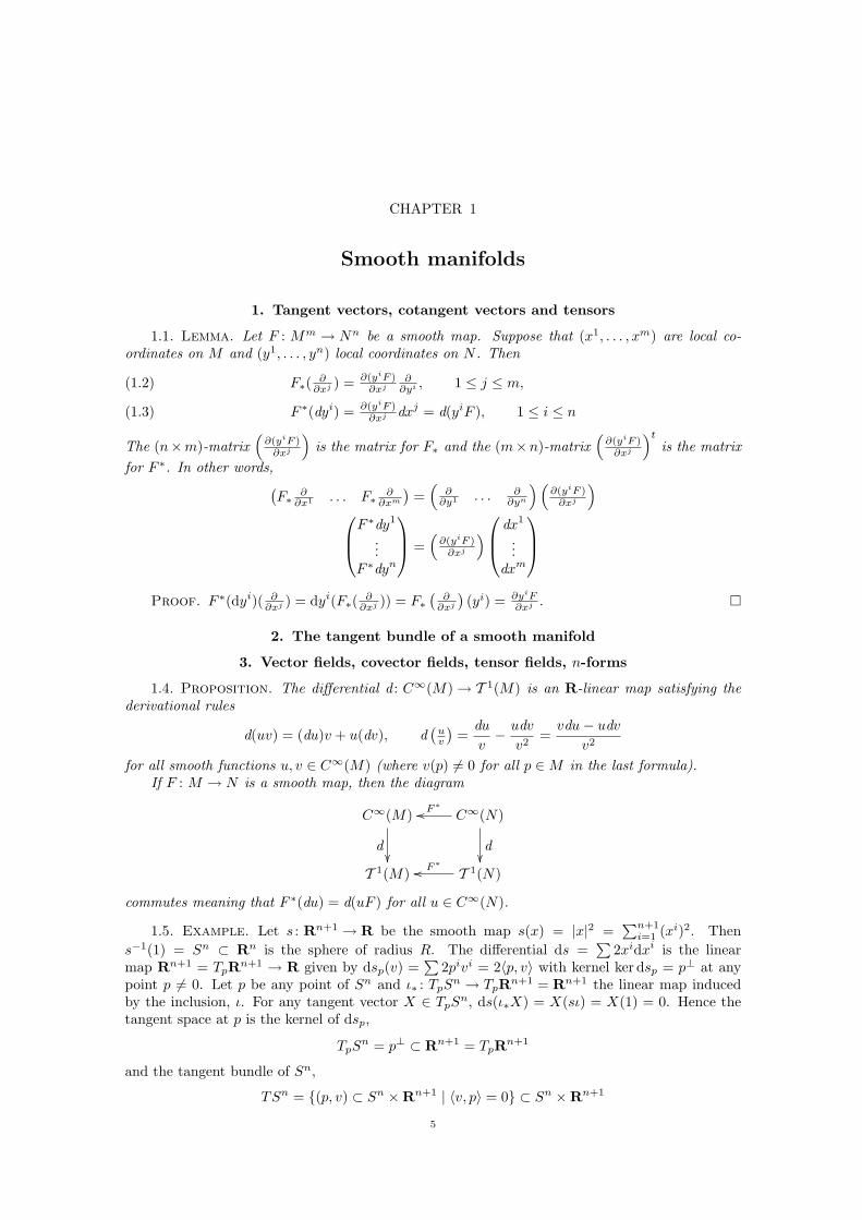
1.1. Lemma. Let F : Mm → Nn be a smooth map. Suppose that (x1, . . . , xm) are local co-ordinates on M and (y1, . . . , yn) local coordinates on N . Then

F∗( ∂∂xj ) = ∂(yiF )

∂xj∂

∂yi , 1 ≤ j ≤ m,(1.2)

F ∗(dyi) = ∂(yiF )∂xj dxj = d(yiF ), 1 ≤ i ≤ n(1.3)

The (n×m)-matrix(

∂(yiF )∂xj

)is the matrix for F∗ and the (m×n)-matrix

(∂(yiF )

∂xj

)t

is the matrixfor F ∗. In other words,(

F∗∂

∂x1 . . . F∗∂

∂xm

)=(

∂∂y1 . . . ∂

∂yn

)(∂(yiF )

∂xj

)F

∗dy1

...F ∗dyn

=(

∂(yiF )∂xj

) dx1

...dxm

Proof. F ∗(dyi)( ∂

∂xj ) = dyi(F∗( ∂∂xj )) = F∗

(∂

∂xj

)(yi) = ∂yiF

∂xj . �

2. The tangent bundle of a smooth manifold

3. Vector fields, covector fields, tensor fields, n-forms

1.4. Proposition. The differential d : C∞(M)→ T 1(M) is an R-linear map satisfying thederivational rules

d(uv) = (du)v + u(dv), d(

uv

)=

duv− udv

v2=vdu− udv

v2

for all smooth functions u, v ∈ C∞(M) (where v(p) 6= 0 for all p ∈M in the last formula).If F : M → N is a smooth map, then the diagram

C∞(M)

d��

C∞(N)F∗oo

d��

T 1(M) T 1(N)F∗oo

commutes meaning that F ∗(du) = d(uF ) for all u ∈ C∞(N).

1.5. Example. Let s : Rn+1 → R be the smooth map s(x) = |x|2 =∑n+1

i=1 (xi)2. Thens−1(1) = Sn ⊂ Rn is the sphere of radius R. The differential ds =

∑2xidxi is the linear

map Rn+1 = TpRn+1 → R given by dsp(v) =∑

2pivi = 2〈p, v〉 with kernel ker dsp = p⊥ at anypoint p 6= 0. Let p be any point of Sn and ι∗ : TpS

n → TpRn+1 = Rn+1 the linear map inducedby the inclusion, ι. For any tangent vector X ∈ TpS

n, ds(ι∗X) = X(sι) = X(1) = 0. Hence thetangent space at p is the kernel of dsp,

TpSn = p⊥ ⊂ Rn+1 = TpRn+1

and the tangent bundle of Sn,

TSn = {(p, v) ⊂ Sn ×Rn+1 | 〈v, p〉 = 0} ⊂ Sn ×Rn+1

5

6 1. SMOOTH manifoldS

is the vector bundle whose fibre over any p ∈ Sn is p⊥. A smooth vector field on Sn is a smoothmap v : Sn → Rn+1 such that v(p) ⊥ p for all p ∈ Sn. Show that any odd sphere has a vector fieldwithout zeros. Does S2 admit a smooth vector field with no zeros? Can you describe TRPn? Canyou describe TM if M = f−1(0) consists of the manifold solutions to the equation f(x) = 0 forsome smooth map f : Rn+1 → R?

1.6. Definition. A smooth(k`

)-tensor field on M is a smooth section of the tensor bundle

T k` (M)→M .

Particular cases are• T 0

0 (M) = C∞(M)• T 0

1 (M) consists of vector fields on M• T 1

0 (M) consists of 1-forms on MTensor fields admit

• T k1`1

(M)× T k1`1

(M) ⊗−→ T k1+k2`1+`2

(M) (tensor product of tensor fields)

• T k+1`+1 (M) tr−→ T k

` (M) (contraction of tensor fields)

1.7. Example. Let ω ∈ T 10 (M) be a 1-form and X ∈ T 0

1 (M) a vector field on M . Then

X ⊗ ω ∈ T 11 (M) is

(11

)-tensor field with contraction tr(X ⊗ ω) = ω(X) (5.7).

In a coordinate patch any(k`

)-tensor field A is (5.5) a C∞(M)-linear combination

(1.8) A = Aj1···j`

i1···ik∂j1 ⊗ · · · ∂j`

⊗ dxi1 ⊗ · · ·dxik

of tensor products of the basis tensor fields and basis 1-forms. The smooth functions Aj1···j`

i1···ikare

called the components of the tensor field A.The tensor algebra ofM is the graded algebra T ∗(M) =

∑∞k=0 T k(M) equipped with the tensor

product T r(M) × T s(M) ⊗−→ T r+s(M). If F : M → N is a smooth map, F ∗ : T k(N)→ T k(M)is the linear map given by F ∗(A)(X1, . . . , Xk) = A(F∗X1, . . . , F∗Xk) for all A ∈ T k(N) and allsmooth vector fields X1, . . . , Xk on M .

1.9. Lemma. T ∗(M) is a graded algebra. F ∗ : T ∗(N)→ T ∗(M) is a homomorphism of C∞(N)-algebras: F ∗(aω ⊗ η) = F ∗(a)F ∗(ω)⊗ F ∗(η).

CHAPTER 2

Riemannian manifolds

Riemann’s idea was that in the infinitely small, on a scale much smaller than the the smallestparticle, we do not know if Euclidean geometry is still in force. Therefore we better not assume thatthis is the case and instead open up for the possibility that in the infinitely small there may be otherlength functions, there may be other inner products on the tangent space! A Riemannian manifoldis a smooth manifold equipped with inner product, which may or may not be the Euclidean innerproduct, on each tangent space.

1. Riemannian metric

2.1. Definition. A Riemannian metric on a smooth manifold M is a symmetric, positive

definite(

20

)-tensor g ∈ T 2

0 (M).

In a coordinate frame we may write

g = gijdxi ⊗ dxj , gij = g(∂i, ∂j)

This means that g(U i∂i, Vj∂j) = gijU

iV j and in particular that

(2.1) 〈∂i, ∂i〉 = gii, 〈∂i, ∂j〉 = gij

Note that there are only 12n(n+ 1) different functions here as gij = gji by symmetry.

2.2. Remark. Since the metric tensor is symmetric, it is traditional to write it in a basis ofsymmetric tensors. The symmetrization of ω ⊗ η is the tensor

ωη =12(ω ⊗ η + η ⊗ ω)

Note that ωη = ηω and that ω2 = ωω = ω ⊗ ω. Observe that

g = gijdxidxj = 2n∑

i=1

gii(dxi)2 + 2∑

1≤i<j≤n

gijdxidxj

2.3. Lemma. Let F : M → N be an immersion and g a Riemannian metric on N .

(1) F ∗g is a Riemannian metric on M .(2) If g = gijdyidyj in a coordinate frame on N , then

F ∗(g)|F−1(U) = gijdyiFdyjF

Proof. It is a general fact that F ∗(g) is a smooth 2-form on M (1.9). F ∗(g) is symmetricbecause g is symmetric and it is positive definite because g is positive definite and F∗ is injective

on each fibre. F ∗(gijdyidyj)(1.9)= gijF

∗dyiF ∗dyj (1.4)= gijdyiFdyjF . �

For instance if F : U →M is a parameterization (an inverse chart) of an open subset of M ⊂Rm, then the pull-back of the induced metric on M is

(2.4) F ∗(g) = F ∗(δijdxidxj) = δijdFidF j =

m∑i=1

(dF i)2

These expressions are tensor fields living in the tensor algebra T ∗(M) of M .

7

http://turnbull.mcs.st-and.ac.uk/history/Mathematicians/Riemann.html

8 2. RIEMANNIAN MANIFOLDS

2.5. Example. (Graphs) Let M ⊂ Rn ×R be the graph of the smooth function f : M → R.Then s(x) = (x, f(x)) is a diffeomorphism so that the Riemannian manifold (M, ι∗gn+1) is isometricto (Rn, s∗gn+1) where the metric s∗gn+1 is

s∗(n+1∑i=1

(dxi)2) =n∑

i=1

(dxi)2 +( ∂f∂xi

dxi)2 =

n∑i=1

(dxi)2 +∂f

∂xi

∂f

∂xjdxidxj

=(δij +

∂f

∂xi

∂f

∂xj

)dxidxj =

n∑i=1

(1 + (

∂f

∂xi)2)(dxi)2 + 2

∑1≤i<j≤n

∂f

∂xi

∂f

∂xjdxidxj

2.6. Example. let S2+ be the upper hemisphere on S2 ⊂ R3 considered as the graph of the

function f(x, y) =√

1− x2 − y2 defined on the unit ball B2 ⊂ R2. Then (S2+, ι

∗g3) is isometricto (B2, s∗g3) where

s∗g3 = (dx)2 + (dy)2 +

(−x√

1− x2 − y2dx+

−y√1− x2 − y2

dy

)2

=1− y2

1− x2 − y2(dx)2 +

1− x2

1− x2 − y2(dy)2 +

2xy1− x2 − y2

dxdy

This means (2.1) that

〈∂x, ∂x〉 =1− y2

1− x2 − y2, 〈∂y, ∂y〉 =

1− x2

1− x2 − y2, 〈∂x, ∂y〉 =

xy

1− x2 − y2

at the point (x, y) ∈ B2. In this metric, the basis tangent vectors, ∂x and ∂y, are not orthogonalat any point of the unit ball away from the axes. If we consider the curve γ(t) = (t, 0), −1 ≤ t ≤ 1,then the tangent vector γ∗( d

dt ) = d(xγ)dt ∂x + d(yγ)

dt ∂y = ∂x so that the length of this curve is

Ls∗(g)(γ) =∫ +1

−1

|γ∗(d

dt)|dt =

∫ +1

−1

√1

1− t2dt = π

What is the distance between (0,−1/2) and (1/2, 0)? What is the curve of shortest length betweenthese two points?

2.7. Example. (Surface of revolution in R3)

2.8. Definition. A smooth map F : (M, g)→ (N,h) between two Riemannian manifolds is anisometry if g = F ∗h; if g(X,Y ) = h(F∗X,F∗Y ) for all tangent vectors X,Y ∈ TpM , p ∈M .

Two Riemannian manifolds are isometric if we can deform one into the other by bending butnot stretching. Is the upper unit hemisphere S2

+ ⊂ R3 isometric to the open unit ball B2 ⊂ R2?Certainly, the diffeomorphism s : B2 → S2

+ from Example 2.6 is not an isometry as for instance〈∂x, ∂x〉 6= 1 or because the tangent vectors ∂x and ∂y are not orthogonal throughout any open(nonempty) subspace of B2. But there are many other diffeomorphisms and maybe we couldfind one that preserves the metrics? To decide if this is the case we need to find invariants ofRiemannian metrics. Is S2

+ curved? And what does that mean? We need to develop some theoryto answer these questions.

In order to decide if two given Riemannian manifolds are isometric we have to know havethe metric tensor transforms under change of coordinate system? (Remember that the coordinateexpression for a metric is an artefact of the coordinate system and not an intrinsic property of themetric.)

2.9. Lemma. Let φ : Rn →M and ψ : Rn →M be parameterizations of the same open subspaceof M . If

φ∗(g) = aijdxidxj , ψ∗(g) = bijdyidyj

then

(aij) =(

∂yi

∂xj

)t

(bij)(

∂yi

∂xj

)where y = ψφ−1.

2. THE THREE MODEL GEOMETRIES 9

Proof. Put P =(

∂yi

∂xj

). Then (1.1)

y∗

dy1

...dyn

= P

dx1

...dxn

Therefore

aijdxidxj = φ∗g = (ψy)∗g = y∗(ψ∗g) = y∗(bijdyidyj)

= y∗((dy1 . . . dyn

)(bij)

dy1

...dyn

)

=(dx1 . . . dxn

)P t(bij)P

dx1

...dxn

so that (aij) = P t(bij)P . �

Suppose that φ∗g = aijdxidxj for some parameterization φ. Is M locally flat? In otherwords, does there exist a re-parameterization ψ = φy of M such that ψ∗g = δijdyidyj? Such are-parameterization exists if and only if the set of 1

2n(n− 1) PDEs

(gij) =(

∂yi

∂xj

)t (∂yi

∂xj

),

or equivalently,

(2.10) gij =n∑

k=1

∂yk

∂xi∂yk

∂xj , 1 ≤ i ≤ j ≤ n,

has a solution y = (y1, . . . , yn). Riemann showed (in an essay that was never properly recognized)that (2.10) is equivalent to

∂2y`

∂xi∂xj= Γk

ij∂y`

∂xk , 1 ≤ i, j, ` ≤ n,

and thereby that (2.10) has a solution if and only if

Rmjk` = 0, 1 ≤ j, k, `,m ≤ n,

where the Γkij (the Christoffel symbols) and the Rm

jk` are certain functions defined in terms of thefunctions gij . This was the birth of the Riemann curvature tensor Rm

jk`! This direct approach,however, is not the one used today since it is conceptually simpler first to introduce a device calleda connection that will enable us to work in a coordinate-free way on M .

2.11. Example. (Cylinders are flat.) Let γ(s) = (x(s), y(s)), a < s < b, be a smooth curve inR2 such that the tangent γ∗( d

ds ) = x′(s)∂x + y′(s)∂y 6= 0 for all t. Let M ⊂ R3 be the cylinderover γ, the surface with parameterization φ(s, t) = (x(s), y(s), z(t)) where z(t) = t. Then (2.3),

φ∗(g3) = (dx)2 + (dy)2 + (dz)2 = (x′(s)ds)2 + (y′(s)ds)2 + (dt)2 = |γ∗(dds

)|2(ds)2 + (dt)2

What are Riemann’s equations in this case? Is there a solution?

2. The three model geometries

The model geometries are Euclidean geometry, spherical geometry, and hyperbolic geometry.


2.1. Euclidean geometry. Euclidean geometry is the geometry of the Riemannian manifold(Rn, gn) where

gn = δijdxidxj =

n∑i=1

(dxi)2

meaning that gn(U i∂i, Vj∂j) =

∑ni=1 U

iV i. (The straight line over the g is to remind you ofEuclidean geometry.)

The isometry group of Euclidean geometry

Isom(Rn, gn) = Aff(n) = Rn o O(n)

acts transitively on Rn by the rule (v,A)(x) = v +Ax. The isotropy subgroup at 0 ∈ Rn is O(n)and the projection

O(n)→ Aff(n) = O(TRn)→ Aff(Rn)/O(n) = Rn

is the unit n-frame bundle of Euclidean geometry Rn.

2.2. Spherical geometry. Spherical geometry is the geometry of the Riemannian manifold(Sn

R, gnR) where

SnR = {(ξ, τ) ∈ Rn ×R | |ξ|2 + τ2 = R2}

is the n-sphere of radius R and gnR = ι∗

(∑ni=1(dξi)

2 + (dτ)2)

is the restriction of the Euclideanmetric on Rn ×R.

The isometry group of spherical geometry

Isom(SnR, gR) = O(n+ 1)

(The smooth action of O(n + 1) ⊂ Aff(n + 1) on Rn+1 restricts to a smooth action on Sn –and in fact these are all isometries.) O(n + 1) acts transitively on Sn. The isotropy subgroup atN = (0, . . . , 0, 1) ∈ Sn is O(n) and the projection

O(n)→ O(TSn) = O(n+ 1)→ O(n+ 1)/O(n) = Sn

is the unit n-frame bundle of spherical geometry Sn.

2.12. Proposition. Stereographic projection σ : SnR −N → Rn is given by

σ(ξ, τ) =R

R− τξ

and the inverse is given by

σ−1(u) = (ξ(u), τ(u)), ξ(u) =2R2u

|u|2 +R2, τ(u) = R

|u|2 −R2

|u|2 +R2

Stereographic projection is a diffeomorphism.

Proof. Elementary. �

2.13. Proposition. The Riemannian manifold (SnR −N, gn

R) is isometric to the Riemannianmanifold (Rn, (σ−1)∗gn

R) where

(σ−1)∗gnR =

4R4

(R2 + |u|2)2gn

is conformally equivalent to the Euclidean metric.

Proof. By 2.3

(σ−1)∗gR =n∑

j=1

(dξj)2 + (dτ)2

2. THE THREE MODEL GEOMETRIES 11

We will now use the derivation rules 1.4. The denominator of ξ and τ is |u|2+R2 and d(|u|2+R2) =d(|u|2) =

∑2ujduj which we shall write as 2〈u, du〉. Because

dξj = d

(2R2u

|u|2 +R2

)=

2R2duj

|u|2 +R2− 4R2uj〈u, du〉

(|u|2 +R2)2

dτ = d

(R|u|2 −R2

|u|2 +R2

)= R

2〈u, du〉(|u|2 +R2)2

−R (|u|2 −R2)2〈u, du〉(|u|2 +R2)2

=2R〈u, du〉(|u|2 +R2)− 2R〈u, du〉(|u|2 −R2)

(|u|2 +R2)2

=4R3〈u, du〉(|u|2 +R2)2

we getn∑

j=1

(dξj)2 =n∑

j=1

(4R4(duj)2

|u|2 +R2+

16R4(uj)2〈u, du〉(|u|2 +R2)4

− 16R4ujduj〈u, du〉(|u|2 +R2)3

)

=4R4(duj)2

(|u|2 +R2)2

n∑j=1

(duj)2 +16R4|u|2〈u, du〉2

(|u|2 +R2)4− 16R4〈u, du〉2

(|u|2 +R2)3

=4R4(duj)2

(|u|2 +R2)2gn +

16R4|u|2〈u, du〉 − 16R4|u|2〈u, du〉2 − 16R6〈u, du〉2

(|u|2 +R2)4

=4R4(duj)2

(|u|2 +R2)2gn − 16R6〈u, du〉2

(|u|2 +R2)4

=4R4(duj)2

(|u|2 +R2)2gn − (dτ)2

�

2.14. Hyperbolic geometry. Hyperbolic geometry is the geometry of the Riemannian man-ifold (Hn

R, hnR) where

HnR = {(ξ, τ) ∈ Rn ×R+ | |ξ|2 − τ2 = −R2}

id the hyperbolic space n-space of radius R and hnR = ι∗

(∑ni=1(dξ

i)2 − (dτ)2)

is the restriction ofthe Minkowski metric on Rn ×R. Let N = (0, . . . , 0, R) ∈ Hn

R be the north pole.

2.15. Remark. (Minkowski metric) Let m be the inner product on Rn+1 with matrix D =diag(1, . . . , 1,−1). We can view m both as an inner product on the vector space Rn (〈X,Y 〉 =m(X,Y ) = XtDY ) or as a Minkowski metric on the manifold Rn+1 (〈Xi∂i, Y

i∂i〉 = m(X,Y )).For each p ∈ Hn

R, the tangent space

TpHnR = p⊥ ⊂ Rn+1 = TpRn+1

exactly as in 1.5.

LetO(n, 1) = {A ∈ GL(n,R) | AtDA = D}

be the group of linear automorphisms of Rn+1 that preserve the inner product. The columns (orrows) of each A ∈ O(n, 1) form an orthogonal basis for Rn+1 of vectors of length 1, . . . , 1,−1.The elements of the Lie group O(n, 1) preserve the subspace {(ξ, τ) ∈ Rn+1 | |(ξ, τ)|2 = −R2} ofvectors of square length −R2. This subspace has two connected components. Let O+(n, 1) be thesubgroup of O(n, 1) consisting of the elements that take the connected component Hn

R to itself.The Lie group O+(n, 1) acts transitively on Hn

R; given any v ∈ HnR, we can find an A ∈ O+(n, 1)

whose last column is 1Rv so that AN = v where N is the north pole. The isotropy subgroup at N

consists of the A ∈ O+(n, 1) whose last column is (0, . . . , 0, 1). The isotropy subgroup, isomorphicto O(n), act transitively on the tangent space TNH

nR. The projection

O(n)→ O(THnR) = O+(n, 1)→ O+(n, 1)/O(n) = Hn

R

is the unit n-frame bundle of HnR.


2.16. Proposition. Hyperbolic stereographic projection π : HnR → Bn

R is given by

π(ξ, τ) =Rξ

R+ τ

and its inverse is given by

π−1(u) = (ξ(u), τ(u)), ξ(u) =2R2u

R2 − |u|2, τ(u) = R

R2 + |u|2

R2 − |u|2

Hyperbolic stereographic projection is a diffeomorphism.

Proof. Elementary. �

2.17. Proposition. The Riemannian manifold (HnR, h

nR) is isometric to the Riemannian man-

ifold (Bn(R), (π−1)∗hnR) where

(π−1)∗(hnR) =

4R4

(R2 − |u|2)2gn

is conformally equivalent to the Euclidean metric.

Proof. By 2.3 (applied to the Minkowski metric)

(σ−1)∗hR =n∑

j=1

(dξj)2 − (dτ)2

Using that d(R2 − |u|2) = −2〈u, du〉 and 1.4 we get

dξj =2R2duj

R2 − |u|2+

2R2uj2〈u, du〉(R2 − |u|2)2

dτ = R2〈u, du〉R2 − |u|2

+R(R2 + |u|2)2〈u, du〉

(R2 − |u|2)2

=2R3〈u, du〉 − 2R|u|2〈u, du〉+ 2R3〈u, du〉+ 2R|u|2〈u, du〉

(R2 − |u|2)2

=4R3〈u, du〉(R2 − |u|2)2

Thereforen∑

j=1

(dξj)2 =n∑

j=1

(2R2duj

R2 − |u|2+

4R2uj〈u, du〉(R2 − |u|2)2

)2

=4R4

(R2 − |u|2)2n∑

j=1

(duj)2 +16R4|u|2〈u, du〉

(R2 − |u|2)4+

16R4〈u, du〉2

(R2 − |u|2)3

=4R4

(R2 − |u|2)2gn +

16R4|u|2〈u, du〉+ 16R6〈u, du〉2 − 16R4|u|2〈u, du〉2

(R2 − |u|2)4

=4R4

(R2 − |u|2)2gn +

16R6〈u, du〉2

(R2 − |u|2)4

=4R4

(R2 − |u|2)2gn + (dτ)2

�

Let Un = {(x, y) ∈ Rn−1 ×R | y > 0} be the upper half plane in Rn.

2.18. Proposition. The Riemannian manifold (HnR, h

nR) is isometric to the smooth manifold

Un equipped with the Riemannian metric R2 1y2 g

n.

Proof. A computation. �

Does the hyperbolic plane H2 embed isometrically in R3? Any Riemannian ma embeds iso-metrically into some Euclidean space [6].

3. CONNECTIONS 13

3. Connections

Let E → M be a smooth vector bundle over M and E(M) the C∞(M)-module of smoothsections. A connection on E is a recipe for how to differentiate a section of E along a vector field.

2.19. Definition. A connection on E is a map

T (M)× E(M) ∇−→ E(M)

(X,Y )→ ∇XY

which is C∞(M)-linear in X and R-linear in Y and satisfies the product rule

∇X(fY ) = (Xf)Y + f∇XY

for all f ∈ C∞(M).

There always are connections, for instance the 0-connection given by ∇XY = 0.

2.20. Lemma. The value ∇XY (p) at the point p ∈M only depends on Y in a neighborhood ofp and X at p.

Proof. Let us first focus on Y -variable. By linearity, it is enough to show that if Y = 0 in aneighborhood U of p, then ∇XY (p) = 0. Choose a smooth bump function φ such that φ(p) = 1and φ = 0 outside U . Then φY is the zero section so that

0 = ∇X0 = ∇X(φY ) = (Xφ)Y + φ∇XY

Evaluating at p, we get 0 = ∇XY (p) since Y (p) = 0 and φ(p) = 1.Next, we focus on the X-variable. By an argument similar to the one just given, we first show

that if X is 0 in a neighborhood of p, then 0 = ∇XY (p). Suppose now that we only know that Xvanishes at the point p, X(p) = 0. Choose a moving frame Ei in a neighborhood of p. Extend thelocally defined vector fields Ei to globally defined smooth vector fields. There are smooth functionsXi such that X = XiEi in a neighborhood of p. Then ∇XY (p) = ∇XiEi

Y (p) since X and XiEi

are equal in a neighborhood of p. By C∞(M)-linearity in X,

∇XiEiY = Xi∇Ei

Y

which evaluated at p is 0 since Xi(p) = 0 for all i. �

We are particularly interested in connections on the tangent bundle of M .

2.21. Definition. A linear connection is a connection T (M)×T (M) ∇−→ T (M) on the tangentbundle of M .

Are there any linear connections, apart from the 0-connection, on M?

2.22. Example. The Euclidean connection ∇X(Y j∂j) = X(Y j)∂j is a nonzero linear connec-tion on Euclidean space M = Rn. Note that ∇∂i

∂j = 0, 1 ≤ i, j ≤ n. A smooth vector fieldY = Y i∂i on Rn is the same thing as a smooth map Y = Y iEi : Rn → Rn. The derivative in thedirection of (tangent) vector X of the map Y = Y iEi is X(Y ) = X(Y i)Ei. For consistency sakewe better declare the derivative of the vector field Y = Y i∂i to be ∇XY = X(Y i)∂i to ensure thatthe diagram

C∞(Rn,Rn) X // C∞(Rn,Rn)

T (Rn)∇X // T (Rn)

commutes.

If we can construct connections on Rn, maybe we can define a connection in each coordinatepatch on M and then put them together? What does a connection look like locally?


2.23. Lemma. Suppose that U is an open subspace of M that admit a moving frame Ei. Thelinear connection ∇ on M restricts to linear connection on U . If X = XiEi and Y = Y jEj arevector fields on U then

∇XY = (XY k +XiY jΓkij)Ek

where the n3 smooth functions Γkij are the Christoffel symbols given by ∇Ei

Ej = ΓkijEk.

Proof. We compute

∇XY = ∇X(Y jEj) = XY jEj + Y j∇XEjXYjEj + Y j∇XiEi

Ej = XY jEj +XiY j∇EiEj

= XY jEj +XiY jΓkijEk = XY kEk +XiY jΓk

ijEk = (XY k +XiY jΓkij)Ek

where we use the Christoffel symbols. �

Thus we see that we can express ∇XY by means of the n3 smooth functions Γkij . Conversely,

for any choice of n3 smooth functions Γkij we can define ∇XY , X,Y ∈ T (U) by the above formula

and that will be a connection. So a linear connection on U is the same thing as a collection of n3

smooth functions on U .In particular if M is a smooth manifold and {Uα} a smooth atlas on M then can find a linear

connection ∇α on each Uα. In order to construct a linear connection on M , let {φα} be a smoothpartition of unity subordinate to {Uα}.

Theorem 2.24. (Existence of connections) Any smooth manifold M has many linear connec-tions:

∇XY =∑α

φα∇αXY

is a linear connection on M .

Armed with a linear connection we know how to differentiate vector fields along vector fields.But as a bonus we can even differentiate arbitrary tensor fields along vector fields!

2.25. Lemma. (Existence and uniqueness of the covariant derivative of a tensor field) LetT (M)× T (M) ∇−→ T (M) be a linear connection on M (2.21). Then there are unique connections

T (M)× T k` (M) ∇−→ T k

` (M)

on all tensor bundles T k` (M)→M such that

(1) ∇Xf = Xf for all f ∈ T 00 (M) = C∞(M)

(2) ∇XY is the given linear connection for all vector fields Y ∈ T 10 (M)

(3) ∇X(A⊗B) = ∇XA⊗B +A⊗∇XB

(4) ∇X trA = tr∇XA for all A ∈ T k+1`+1 (M)

Namely, for any 1-form ω, ∇Xω is the 1-form given by

(2.26) (∇Xω)(Y ) = X(ω(Y ))− ω(∇XY )

and, in general, for any(k`

)-tensor A ∈ T k

` (M), ∇XA is the(k`

)-tensor given by

(2.27) (∇XA)(ω1, . . . , ω`, Y1, . . . , Yk) = X(A(ω1, . . . , ω`, Y1, . . . , Yk))

−k∑

i=1

A(ω1, . . . , ω`, Y1, . . . ,∇XYi, . . . , Yk)−∑j=1

A(ω1, . . . ,∇Xωj , . . . , ω`, Y1, . . . , Yk)

for any choice of k vector fields Y1, . . . , Yk and ` 1-forms ω1, . . . , ω` on M .

Proof. Let’s assume that we have connections that satisfy items (1)–(4). What is the cov-ariant derivative of a 1-form ω? For any two vector fields X and Y ,

X(ω(Y ))(1)= ∇X(ω(Y ))

(1.7)= ∇X(tr(ω ⊗ Y ))

(4)= tr∇X(ω ⊗ Y )

(3)= tr(∇Xω ⊗ Y + ω ⊗∇XY )

(1.7)= (∇Xω)(Y ) + ω(∇XY )

3. CONNECTIONS 15

which is (2.26). So we are forced to define ∇Xω as in (2.26). But then there is at most onepossibility for ∇XA since any tensor is a sum of a smooth function times tensor products of vectorfields and 1-forms (combine the local expression (1.8) for a tensor with a smooth partition of unity).This shows uniqueness.

To show existence, use (2.26) to define the covariant derivative of a 1-form and then use (2.27)to define ∇XA in general. Check that this definition satisfies (1)–(4). �

2.28. Definition. The total covariant derivative ∇ : Tk` (M)→ Tk+1

` (M) is given by

∇A(ω1, . . . , ω`, Y1, . . . , Yk, X) = (∇XA)(ω1, . . . , ω`, Y1, . . . , Yk)

for all A ∈ T k` (M).

Note that the total covariant derivative of the tensor field A ∈ T k` (M) is zero if and only if

the covariant derivative of A along all vector fields is zero: ∇A = 0 ⇐⇒ ∀X ∈ T (M) : ∇XA = 0.

2.29. Example. There are total covariant derivatives

C∞(M) = T 00 (M) ∇−→ T 1

0 (M) ∇−→ T 20 (M) ∇−→ T 3

0 (M) ∇−→ · · ·

If u ∈ C∞(M) is a smooth function and X a vector field, then

(∇u)(X) = ∇X(u) = X(u) = du(X)

so that ∇u = du.The 2-form ∇2u = ∇∇u is called the covariant Hessian of u. If X and Y a vector fields, then

(∇2u)(Y,X) = (∇∇u)(Y,X)(2.28)= (∇X∇u)(Y )

(2.26)= X((∇u)(Y ))−∇u(∇XY )

∇u=du= X(Y (u))− (∇XY )(u)

Consequently,∇2u = 0 ⇐⇒ ∀X,Y ∈ T (M) : Y (X(u)) = (∇Y X)(u)

2.30. Example. If g ∈ T 20 (M) is the Riemannian metric, then ∇g is the 3-form given by

(∇g)(X,Y, Z)(2.28)= (∇Zg)(X,Y )

(2.27)= Zg(X,Y )− g(∇ZX,Y )− g(X,∇ZY )

for any three vector fields X,Y, Z. Consequently

∇g = 0 ⇐⇒ ∀X,Y, Z ∈ T (M) : Z〈X,Y 〉 = 〈∇ZX,Y 〉+ 〈X,∇ZY 〉

for all vector fields X,Y, Z.

2.31. Example. There are total covariant derivatives

T (M) = T 01 (M) ∇−→ T 1

1 (M) ∇−→ T 21 (M) ∇−→ · · ·

If V ∈ T 01 (M) is a vector field then ∇V is the

(11

)-tensor given by

(∇V )(ω,X) = (∇XV )(ω) = ω(∇XV )

If V = V i∂i in local coordinates, then

(∇V )(dxi, ∂j) = dxi(∇∂jV ) = dxi(∇∂j

V k∂k) = dxi(∂jVk∂k + V kΓ`

jk∂`) = ∂jVi + V kΓi

jk

and therefore∇V = (∂jV

i + V kΓijk)∂i ⊗ dxj

We say that the vector field V is parallel if ∇V = 0. Since

∇V = 0 ⇐⇒ ∀X ∈ T (M) : ∇XV = 0,

V is parallel iff the covariant derivative of V along any vector field is zero. What tensor is ∇2V ?What does it mean if ∇2V = 0?


4. Geodesics and parallel translation along curves

Let γ : I →M be a smooth curve on M .

2.32. Definition. For any t ∈ I, the tangent vector

•γ (t) = γ∗(

ddt

(t)) ∈ Tγ(t)M,•γ (t)f =

d(f ◦ γ)dt

(t), f ∈ C∞(M)

is called the velocity vector of γ at the point γ(t).

If x is a coordinate system around γ(t0) and xγ = (γ1, . . . , γn) then

(2.33)•γ (t) =

dγi

dt(t)∂i(γ(t))

as a special case of (1.2).

2.34. Remark. We say that the curve γ, defined in an open neighborhood of 0, representsthe tangent vector V ∈ TpM if γ(0) = p and

•γ (0) = V . Then V f =

•γ (0)f = d

dt (fγ)(0) for anysmooth function f ∈ C∞(M) and F∗V is represented by the image curve Fγ for any smooth mapF : M → N .

2.35. Definition. A vector field along γ is a smooth map V : I → TM such that the diagram

TM

��I

V

=={{{{{{{{γ

// M

commutes. A vector field V along is extendible if V (t) = V (γ(t)) for some vector field V on aneighborhood of γ(I). The C∞(I)-module of all vector fields along γ is denoted T (γ).

The velocity field•γ (t) is an example of a vector field along γ.

The formulation of the lemma below makes use of 2.20.

2.36. Lemma (Covariant differentiation along a curve). Let ∇ be a connection on M . Thereexists precisely one R-linear map Dt : T (γ)→ T (γ) such that

Dt(fV ) =dfdtV + fDtV, f ∈ C∞(I), V ∈ T (γ)

DtV = ∇•γ(t)

V V extendible

• If Ei is a local frame around γ(t0) and V = V jEj, then

DtV =dV j

dtEj + V j∇•

γ(t)Ej

for t near t0.• If x is a coordinate system around γ(t0) and V = V j∂j, then

DtV = (dγk

dt+ Γk

ij

dγi

dtV j)∂k

for t near t0.

A curve on M is as close as possible to being a straight line if the curve at all times justcontinues in the direction of

•γ (t), if its velocity

•γ (t) does not change. No change means zero

covariant derivative.

2.37. Definition. A smooth curve γ is a geodesic (with respect to the connection ∇) if the

covariant derivative of its velocity field vanishes, Dt

•γ= 0.

A geodesic is a curve that follows its own nose. A geodesic is a curve with constant velocity.Light rays follow geodesics in space-time.

5. THE Riemannian CONNECTION 17

If x is a coordinate system around some point γ(t0) of γ, then γ is a geodesic iff

(2.38)d2γk

dt2+ Γk

ij

dγi

dtdγj

dt= 0

near t0. In principle, we could determine geodesics by solving this equation. In practice, this isclose to impossible. Instead we try to identify some properties that a geodesic must have (2.54,2.58).

2.39. Proposition (Existence and uniqueness of geodesics). Let p be a point on M andV ∈ TpM a tangent vector at p There exists a unique maximal geodesic γV : I →M defined on an

open interval containing 0 such that γV (0) = p and•γV (0) = V .

2.40. Lemma (Rescaling lemma). Let V ∈ TpM be a tangent vector at p ∈ M and let c ∈ Rbe a real number. The geodesic γcV is defined at t iff the geodesic γV is defined at ct and thenγcV (t) = γV (ct).

Proof. Consider the maximal geodesic γV : I →M . Put γ(t) = γV (ct) for all t ∈ c−1I. Thenγ(t) is a geodesic because it satisfies (2.38) in any coordinate system and it is defined at c−1t. In

fact, γ(t) = γcV (t) as γ(0) = γV (0) = p and•γ (0) = cV . �

A vector field along a curve is parallel if it doesn’t change; no change meaning zero covariantderivative. A curve is a geodesic if it has a parallel velocity field.

2.41. Definition. A vector field V along γ is parallel if it does not change along γ, DtV = 0.

2.42. Proposition. Let γ be a curve on M . Suppose that p0 = γ(t0) is a point on γ andV0 ∈ Tp0M a tangent vector at that point. There exists precisely one parallel vector field V alongγ such that V (t0) = V0.

5. The Riemannian connection

On a Riemannian manifold there is a preferred connection.

Theorem 2.43 (The fundamental theorem of Riemannian geometry). A Riemannian manifoldadmits precisely one symmetric connection compatible with the metric.

This particular connection is called the Riemannian connection or the Levi–Civitta connection.

2.44. Definition. The connection ∇ is symmetric if

∇XY −∇Y X = [X,Y ]

for all vector fields X,Y ∈ T (M).

2.45. Lemma. Let Ei be a local moving frame such that [Ei, Ej ] = 0, 1 ≤ i, j ≤ n (for instanceEi = ∂i could be a coordinate frame). Then ∇ is symmetric if and only if

Γkij = Γk

ji, 1 ≤ i, j, k ≤ n

Proof. ∇EiEj −∇Ej

Ei = (Γkij − Γk

ji)Ek. �

2.46. Definition. The connection ∇ is compatible with the metric g if

X 〈Y,Z〉 = 〈∇XY, Z〉+ 〈X,∇XZ〉

for any three vector fields X,Y, Z ∈ T (M).

2.47. Lemma. Let Ei be a local moving frame. Then ∇ is compatible with the metric g if andonly if

Ekgij = Γ`kigj` + Γ`

kjgi`, 1 ≤ i, j, k, ` ≤ n

Proof. Ek 〈Ei, Ej〉 − 〈∇EkEi, Ej〉 − 〈Ei,∇Ek

Ej〉 = Ekgij − Γ`kigj` − Γ`

kjgi`. �


Proof of Theorem 2.43. We first show uniqueness. Assume that ∇ is a symmetric con-nection that is compatible with g. Then

X 〈Y, Z〉 2.44= 〈∇XY,Z〉+ 〈Y,∇XZ〉2.46= 〈∇XY,Z〉+ 〈Y,∇ZX〉+ 〈Y, [X,Z]〉

for any three vector fields X,Y, Z ∈ T (M). Permute X,Y, Z cyclically, obtain

X 〈Y, Z〉 − Z 〈X,Y 〉+ Y 〈X,Z〉 = 2 〈∇XY, Z〉+ 〈Y, [X,Z]〉 − 〈X, [Z, Y ]〉+ 〈Z, [Y,X]〉

and conclude that

(2.48) 〈∇XY, Z〉 =12

(X 〈Y, Z〉 − Z 〈X,Y 〉+ Y 〈X,Z〉 − 〈Y, [X,Z]〉+ 〈X, [Z, Y ]〉 − 〈Z, [Y,X]〉)

This equation shows that ∇, if it exists, is determined by the metric.Next, we show existence. We will define ∇ in any open submanifold where we have a moving

frame Ei with [Ei, Ej ] = 0 (for instance in a chart domain). The only possibility is to put

(2.49) Γkij =

12gk` (Eigj` − E`gij + Ejgi`)

because

(2.50) Γkijgk` = 〈∇Ei

Ej , E`〉 =12

(Eigj` − E`gij + Ejgi`)

by equation (2.48). Since Γkij = Γk

ji and

Γ`kigj`+Γ`

i`gi` = Γ`kig`j +Γ`

i`gì2.50=

12

(Ekgij − Ejgik + Eigjk)+12

(Ekgij − Eigjk + Ejgik) = Ekgij

this connection ∇ is symmetric and compatible with g (2.45, 2.47). �

2.51. Example. The Euclidean connection ∇ (2.22) is the Riemannian connection on Euc-lidean space Rn for it is symmetric and compatible with the Euclidean metric g (2.1) since Γk

ij = 0.

What is the Riemannian connection in spherical and hyperbolic space?

2.52. Lemma. Let ∇ be a connection and g a metric on M . The following conditions areequivalent:

(1) ∇ and g are compatible (2.46)(2) ∇g = 0(3) d

dt 〈V,W 〉 = 〈DtV,W 〉+ 〈V,DtW 〉 whenever V,W are vector fields along a smooth curve(4) 〈V,W 〉 is constant whenever V,W are parallel vector fields along a smooth curve(5) Parallel transport is an isometry

Proof. (1) ⇐⇒ (2): 2.30(3) =⇒ (4) =⇒ (5) : Obvious.(5) =⇒ (3) : Let P1, . . . , Pn be parallel vector fields that are orthonormal at one point of the curveand hence orthonormal at any point. Write V = V iPi and W = W iPi. Then 〈V,W 〉 =

∑V iW i

and (2.36) DtV = dV i

dt Pi and DtW = dW i

dt Pi. Hence

〈DtV,W 〉+ 〈V,DtW 〉 =∑ dV i

dtW i +

∑V i dW

i

dt=

ddt

∑V iW i =

ddt〈V,W 〉

(3) =⇒ (1) : Let Y and Z be smooth vector fields on M and let γ be a smooth curve, γ(0) = p,•γ (0) = X(p). Then

Xp 〈Y, Z〉 =•γ (0) 〈Y, Z〉 =

ddt〈Y,Z〉 = 〈DtY,Z〉+ 〈Y,DtZ〉 =

⟨∇Xp

Y, Z⟩

+⟨Y,∇Xp

Z⟩

(1) =⇒ (3) : Let p = γ(0), choose a vector field X with X(p) =•γ (0), and choose an orthonormal

moving frame, Ei, around p. Then

0 = X 〈Ei, Ej〉 = 〈∇XEi, Ej〉+ 〈Ei,∇XEj〉

6. CONNECTIONS ON SUBMANIFOLDS AND PULL-BACK CONNECTIONS 19

since ∇ and g are compatible Write V = V iEi and W = W jEj . Then DtV =•V i Ei + V i∇XEi,

and similarly for W , at the point p (2.36). Therefore,

〈DtV,W 〉+ 〈V,DtW 〉 = (•V i W j + V i

•W j) 〈Ei, Ej〉+ V iW j(〈∇XEi, Ej〉+ 〈Ei,∇XEj〉)

=∑

(•V i W i + V i

•W i) =

ddt

∑V iW i =

ddt〈V,W 〉

�

2.53. Lemma (Covariant differentiation commutes with lowering and raising of indices (5.2)).If the connection ∇ is compatible with the metric then the diagram

T k+1` (M)

∇X

��

] // T k`+1(M)

∇X

��

[oo

T k+1` (M)

] // T k`+1(M)

[oo

commutes for any vector field X.

Proof. It will be enough to prove this for vector fields (k = 0 = `)). Suppose that X,U, Vare vector fields. The claim is ∇X(V [) = (∇XV )[. We compute

(∇X(V ])(U) = X(V ])−V ](∇XU) = X 〈U, V 〉−〈∇XU, V 〉 = 〈∇XU, V 〉+〈U,∇XV 〉−〈∇XU, V 〉

= 〈U,∇XV 〉 = (∇XV )](U)

using (2.26) and (2.46). �

2.54. Corollary. Riemannian geodesics have constant speed.

Proof. ddt |

•γ (t)|2 = d

dt 〈•γ (t),

•γ (t)〉 = 2〈Dt

•γ (t),

•γ (t)〉 = 0. �

6. Connections on submanifolds and pull-back connections

Let (M, g) be a Riemannian manifold and M ⊂ M be an embedded submanifold. Supposethat we have a connection ∇ on M . How can we obtain a connection on the submanifold M?

For any tangent vector Xp ∈ TpM , let XTp ∈ TpM denote the orthogonal projection of Xp.

2.55. Proposition (Existence of uniqueness of tangential connections). There exists preciselyone connection ∇T on M such that

∇TXY =

(∇XY

)Twhenever X,Y are vector fields on M and X,Y their restrictions to M . If ∇ is the Riemannianconnection on M , then ∇T is the Riemannian connection on M .

2.56. Lemma. Let ∇ be a connection and let X,Y ∈ T (M) be vector fields on M . Then∇XY (p) only depends on X(p) and Y along a curve tangent to X(p).

Proof. ∇XY (p) = ∇•γ(0)

Y (p) = DtY (0) for any curve γ : (−ε, ε)→M with γ(0) = p and•γ (0) = X(p). �

2.57. Proposition (Pull-back connections). Let φ : M →M be a diffeomorphism and ∇ aconnection on M .

Let (also) ∇ be the map that makes the diagram

T (M)× T (M)

φ∗×φ∗ ∼=��

∇ //___ T (M)

φ∗∼=��

T (M)× T (M)∇ // T (M)

commutative. Thus φ∗∇XY = ∇φ∗Xφ∗Y for all X,Y ∈ T (M).


(1) ∇ is a connection on M .(2) Covariant differentiation wrt ∇ makes the diagram

T (γ)Dt //

φ∗ ∼=��

T (γ)

φ∗ ∼=��

T (φγ)Dt

// T (φγ)

commutative. Thus φ∗DtV = Dtφ∗V for any vector field V along the curve γ in M .(3) Assume that M and M are Riemannian manifolds and that φ is an isometry. If ∇

the Riemannian connection on M , then ∇ is the Riemannian connection on M . Thusφ∗∇XY = ∇φ∗Xφ∗ for all X,Y ∈ T (M).

2.58. Corollary. Isometries of Riemannian manifolds take Riemannian geodesics to Rieman-nian geodesics.

Proof. Let φ : (M, g)→ (M, g) be an isometry of Riemannian manifolds. Then the connec-tion on M is the pull-back of the connection on M (2.57.(3)). Let γV , V ∈ TpM , be a geodesic onM . Then

Dt((φγV )•) = Dt(φ∗•γ)

2.57.(2)= φ∗Dt(

•γ) = φ∗0 = 0

so that φγV = γφ∗V . �

7. Geodesics in the three geometries

We determine the geodesics in Euclidean, spherical, and hyperbolic geometry.

2.59. Euclidean geometry. The Riemannian connection on Rn is the Euclidean connection(2.22).

Let p = (0, . . . , 0) ∈ Rn and V = (1, 0, . . . , 0) ∈ TpRn. We know that there is a uniquemaximal geodesic γV running through p with velocity V . We also know that φγV = γV for anyisometry φ ∈ O(n) of Rn preserving (p, V ). The map φ(ξ1, ξ2, ξ3, . . . , ξn) = (ξ1,−ξ2, ξ3, . . . , ξn)is such an isometry (it is a diffeomorphism and it preserves |ξ|). Thus γV must have ξ2γV = 0.Similarly, ξ3γV = 0, . . . , ξnγV = 0. Thus γV must run along the ξ1-axis. Since it has constantspeed and

•γV (0) = V , we must have

γV (t) = (t, 0, . . . , 0)

This was just one geodesic! But since Rn is homogeneous and isotropic, we have in fact determinedall geodesics: The geodesics in Euclidean geometry are the straight lines. For any point not on ageodesic there is a unique geodesic passing through that point parallel to the given geodesic.

2.60. Spherical geometry. The Riemannian connection on

SnR = {(ξ, τ) ∈ Rn ×R | |ξ|2 + τ2 = R2} ⊂ Rn+1

is the tangential connection (2.55) arising from the Euclidean connection on ambient Rn+1.Let N = (0, . . . , R) ∈ Sn

R be the North Pole and V = (1, 0, . . . , 0) ∈ TN§nR. What is γV , thegeodesic running through N with velocity V ? Using the isometries that change sign on ξi for2 ≤ i ≤ n we see, as above, that γV must run in the intersection of Sn

R and the ξ1τ -plane. Thus

(2.61) γV (t) = (R sin(t/R), 0, . . . , 0, R cos(t/R))

We conclude that the geodesics in spherical geometry are great circles, the intersection of SnR with

planes through the origin. For any point not on a geodesic there is a no geodesic passing throughthat point parallel to the given geodesic.

8. THE EXPONENTIAL MAP AND NORMAL COORDINATES 21

2.62. Hyperbolic geometry. The Riemannian connection on

HnR = {(ξ, τ) ∈ Rn ×R+ | |ξ|2 − τ2 = −R2} ⊂ Rn+1

is the tangential connection (2.55) arising from the Euclidean connection, considered as the Rieman-nian connection of Minkowski metric |(ξ, τ)|2 = |ξ|2 − τ2, on ambient Rn+1.

Let N = (0, . . . , R) ∈ SnR be the North Pole and V = (1, 0, . . . , 0) ∈ TN§nR. What is γV , the

geodesic running through N with velocity V ? Using the isometries that change sign on ξi for2 ≤ i ≤ n we see, as above, that γV must run in the intersection of Hn

R and the ξ1τ -plane. Thus

(2.63) γV (t) = (R sinh(t/R), 0, . . . , 0, R cosh(t/R))

We conclude that the geodesics in hyperbolic geometry are great hyperbolas, the intersection ofHn

R with planes through the origin. (The isometry group O(n, 1)+ takes planes through the origin,u⊥, to planes through the origin.) For any point not on a geodesic there are uncountably manygeodesic passing through that point parallel to the given geodesic.

8. The exponential map and normal coordinates

Let M be a Riemannian manifold with Riemannian connection ∇ (2.43). Put

E = {V ∈ TM | γV is defined at 1}

where γV , V ∈ TpM , is the geodesic through γ(0) = p with velocity•γ (0) = V (2.39). We define

(2.64) exp: E →M by exp(V ) = γV (1)

meaning that exp(V ) is obtained by following the geodesic with initial velocity vector V for onetime unit. We let expp denote the restriction of exp to Ep = E ∩ TpM .

2.65. Proposition (Properties of the exponential map). Let exp: E →M be the exponentialmap on the manifold M .

(1) E is an open subspace of TM and exp: E →M is a smooth map.(2) Ep is star-shaped around 0 for each p ∈M .(3) expp : Ep →M takes straight lines through 0 ∈ TpM to geodesics through p: expp(tV ) =

γV (t) (where both functions are defined for the same set of ts).(4) (expp)∗ : T0TpM = TpM → TpM is the identity map.(5) The exponential map commutes with isometries: The diagram

TpM

expp

��

φ∗ // TpM

expφ(p)

��M

φ// M

commutes for any isometry φ : M →M .

Proof. We defer the proof of (1). Let V ∈ TpM and t ∈ R. Then

tV ∈ Ep ⇐⇒ expp is defined at tV ⇐⇒ γtV is defined at 1 ⇐⇒ γV is defined at t

and for such a t, expp(tV ) = γtV (1) = γV (t) by the Rescaling lemma (2.40). In particular,

V ∈ Ep ⇐⇒ γV is defined at 1 =⇒ γV is defined at s ⇐⇒ sV ∈ Epwhen 0 < s ≤ 1. Thus Ep is star-shaped around 0. Assuming that Ep is open in TpM and that expp

is smooth we now compute the differential of expp. Since the tangent vector V ∈ T0TpM = TpMis (2.34) represented by the image curve t→ tV , (expp)∗ is represented by curve exp(tV ) = γV (t)

with•γV (0) = V . Thus (expp)∗V = V . If φ : M →M is an isometry, then φγV = γφ∗V (2.58) so

that φ expp(V ) = φγV (1) = γφ∗V (1) = expφ(p)(φ∗V ).The geodesic vector field G on TM is the defined by

G(V )f =ddt

∣∣∣t=0

(f•γV (t)), f ∈ C∞(TM)


where•γV(t) is curve on TM obtained by taking the velocity of the geodesic γV . Note that

γV (t0 + t) = γ•γV (t0)

(t) so that

G(•γV (t0))f =

ddt

∣∣∣t=0

f(•γV (t+ t0)) =

ddt

∣∣∣t=t0

f(•γV (t))

where t0 is an arbitrary point in the open interval of definition for γV . This means that integralcurves for the vector field G are velocity fields along geodesics. By a general theorem, there existsa smooth map θ : O → TM , defined on an open subspace O ⊂ R× TM containing 0× TM , suchthat θ(t, V ) is the maximal integral curve for G through V ∈ TM at time t = 0. Hence

E = {V ∈ TM | (1, V ) ∈ O} = i−11 O, i1(V ) = (1, V ),

is open and exp(V ) = πθ(1, V ) is smooth as a composition of smooth maps (π : TM →M is theprojection). �

2.66. Example. Let N = (0, 0, 1) be the North Pole of S2 ⊂ R3 and let V be a unit vectorin the tangent space TNS

2 = N⊥. The exponential map expN : TNS2 = N⊥ → S2 takes the unit

speed radial line tV to the unit speed geodesic whose trace is the intersection of S2 with the planethrough 0 ∈ R3 containing N and V .

Normal coordinates is special coordinate system determined by the metric.Let Up ⊂ TpM be an open subset, star-shaped around 0, of the tangent space such that

expp : Up → U is a diffeomorphism between Up and an open subset U of M . Choose an orthonormalbasis Ei for TpM (with inner product gp) and an orthonormal basis ei for Rn (with standard innerproduct g). Let E : (Rn, g)→ (TpM, gp) be the isometry given by Eei = Ei. Then

(2.67) x = E−1 ◦ exp−1p : M ⊃ U → x(U) ⊂ Rn M

x

66TpMexppoo RnEoo

are normal coordinates around p. (We will often forget to mention E so that V can stand for atangent vector V ∈ TpM as well as a vector V ∈ Rn.) The smooth function

(2.68) r : U − p→ R, r(q) = |x(q)| =√∑

xi(q)2 = |V |g (expp(V ) = q)

is the radial distance function and the unit radial vector field on U − p, denoted

(2.69)∂

∂r(q), q ∈ U − p,

is the vector field formed by the velocity vectors of the unit speed radial geodesic; to any q ∈ U −pit associates the velocity of the unit speed radial geodesic through q.

If BR(0) ⊂ Up, then

BR(p) = expp(BR(0)) = {q ∈ x(U) | r(q) ≤ R}BR(p) = expp(BR(0)) = {q ∈ x(U) | r(q) < R}SR(p) = expp(∂BR(0)) = {q ∈ x(U) | r(q) = R}

is a (closed) geodesic ball , respectively, a geodesic sphere around p. (Make a drawing of thesituation!)

2.70. Proposition (Properties of normal coordinates). Let x : U → x(U) be normal coordin-ates (2.67) around p.

(1) x(γEV (t)) = tV for all V ∈ TpM and for all small t. (In normal coordinates, the geodesicsthrough p are straight lines through 0.)

(2) x(p) = 0, ∂∂xi (p) = Ei, gij(p) = δij, Γk

ij(p) = 0, ∂kgij(p) = 0.

(3) ∂∂r = xi(q)

r(q)∂

∂xi for all q ∈ U − p.

Proof. (1) x−1(tV ) = expp(tEV ) = γEV (t).

(2) x−1(0) = expp(0) = p. Let γ(t) = x−1(tei) be the ith coordinate axis. Then•γ (t) = ∂

∂xi (γ(t))in general (2.33). In this case, γ(t) = x−1(tei) = expp(tEi) = γEi

(t) is the geodesic through

γ(0) = p with velocity•γ (0) = Ei. Thus Ei = ∂

∂xi (p). The components of the Riemannian metric

8. THE EXPONENTIAL MAP AND NORMAL COORDINATES 23

g at p are gij(p) = g( ∂∂xi (p), ∂

∂xj (p)) = g(Ei, Ej) = δij . The radial curve γ(t) = x−1(t(ei + ej)) isa geodesic so its coordinates γk satisfy the ODEs (2.38) which in this particular case means thatΓk

ij(γ(t)) = 0 for all t. For t = 0, we get Γkij(p) = 0. In other words, ∇∂i

∂j(p) = 0 for all i, j. Thenalso

∂kgij(p) = ∂k 〈∂i, ∂j〉 (p) = 〈∇∂k∂i(p), ∂j(p)〉+ 〈∂i(p),∇∂k

∂j(p)〉 = 0 + 0 = 0

since the Riemannian connection is compatible with the Riemannian metric (2.46).(3) Let q ∈ U − p. Suppose that x(q) = V ∈ Rn. Then xi(q) = V i and r(q) = |x(q)| = |V | (2.68).The unit speed radial geodesic from p to q is γ(t) = expp(tV/|V |), 0 ≤ t ≤ |V |. Its velocity vector

is•γ (t) = V i

|V |∂

∂xi (γ(t)) (2.33); at q, in particular, its velocity is V i

|V |∂

∂xi (q) = xi(q)r(q)

∂∂xi (q). �

Let Γ: (−ε, ε)× [a, b]→M be a variation of the curve γ(t) = Γ(0, t). We write (s, t) for pointsin (−ε, ε)× [a, b] (so that the interval [a, b] is placed on the vertical t-axis!). Let Γs(t) = Γ(s, t) =Γt(s) so that Γs is a a curve in the t-direction (a main curve) and Γt is a curve in the s-direction(a transverse curve). Let

∂tΓ(s, t) =ddt

Γs(t) =•Γs (t) = Γ∗(

∂

∂t), ∂sΓ(s, t) =

dds

Γt(s) =•Γt (s) = Γ∗(

∂

∂s),

be the velocities of the main, respectively, the transverse curves. We may view the main velocityfield ∂tΓ as a vector field along a transverse curve Γt and consider its covariant derivative Ds∂tΓalong Γt. Similarly, we may view the transverse velocity field ∂sΓ as a vector field along a maincurve Γs and consider its covariant derivative Dt∂sΓ along Γs.

2.71. Lemma (Symmetry Lemma). Ds∂tΓ = Dt∂sΓ or Ds

•Γs= Dt

•Γt.

Proof. This is a local question. Choose a coordinate system x around Γ(s0, t0). In local

coordinates, xΓ(s, t) = (Γ1(s, t), . . . ,Γn(s, t)) and (2.33) ∂t =•Γs= ∂Γi

∂t ∂i, ∂s =•Γt= ∂Γi

∂s ∂i. In localcoordinates there is a formula for the covariant derivative along a curve (2.36). Using that formula,we get that

Ds∂tΓ =(∂2Γk

∂s∂t+ Γk

ij

∂Γi

∂s

∂Γj

∂t

)∂k

and there is a similar formula for Dt∂Γt except that the s and t swap places. The point is nowthat the Riemannian connection is symmetric so that the Christoffel symbols are symmetric in iand j (2.45). �

The variational field

(2.72) V (t) =•Γt (t, 0) = Γ∗(0,t)(

∂

∂s)

is the restriction to γ(t) of the transverse vector field•Γt.

2.73. Lemma (First Variation of smooth curves). ddsL(Γs)(0) =

⟨V,

•γ⟩ ∣∣∣b

a−∫ b

a

⟨V,Dt

•γ⟩dt

when γ(t) is a unit speed curve.

Proof. We differentiate the function s→ L(Γs) and then evaluate the result at s = 0. Usingthat the connection is compatible with the metric (2.52) and The Symmetry lemma we get

ddsL(Γs) =

dds

∫ b

a

|•Γs (t)|dt =

∫ b

a

∂

∂s

⟨•Γs,

•Γs

⟩1/2

dt2.52=

∫ b

a

1

|•Γs |

⟨Ds

•Γs,

•Γs

⟩dt

2.71=∫ b

a

1

|•Γs |

⟨Dt

•Γt,

•Γs

⟩dt


When s = 0,•Γs=

•Γ0=

•γ, |

•γ | = 1, and

•Γs (0, t) = V (t) so that

ddsL(Γs)(0) =

∫ b

a

⟨DtV,

•γ⟩dt

2.52=∫ b

a

(ddt

⟨V,

•γ⟩−⟨V,Dt

•γ⟩)

dt

=⟨V (b),

•γ (b)

⟩−⟨V (a),

•γ (a)

⟩−∫ b

a

⟨V,Dt

•γ⟩dt

�

2.74. Lemma (Gauss lemma). In a normal neighborhood of a point p we have:

(1) The geodesic spheres are orthogonal to the geodesic rays.(2)

⟨∂∂r , Y

⟩= Y (r) = dr(Y ) for any tangent vector Y ∈ TqM , q 6= p (In other words,

grad r = ∂∂r ).

Proof. Let q = expp(V ) where V 6= 0. Then x(q) = V and r(q) = |V | = R. The claim isthat

W ⊥ V =⇒ (expp)∗W ⊥•γV (1)

for any W ∈ TV TpM = TpM (where V ⊥ = TV SR(0)). Let σ(s) be a curve in SR(0) that representsW , σ(0) = V ,

•σ (0) = W . Consider the variation Γ(s, t) = expp(tσ(s)) of γV (t) = expp(tV ). Put

S = ∂sΓ and T = ∂tΓ. Note that the curves in the t-direction, t → expp(tσ(s)), are geodesics ofvelocity T and speed |T | = |σ(s)| = R. Hence DtT = 0 and |T | = R is constant. It follows that

∂

∂t〈S, T 〉 (2.52)

= 〈DtS, T 〉+ 〈S,DtT 〉 = 〈DtS, T 〉(2.71)= 〈DsT, T 〉

(2.52)=

12∂

∂s|T |2 = 0

where we use that the connection is compatible with the metric and symmetric. Thus

〈S, T 〉(0, 0) = 〈S, T 〉(0, 1)

since 〈S, T 〉(s, t) is independent of t. We know compute

S(0, 0) =•Γ0 (0) = 0, S(0, 1) =

•Γ1 (0) = (expp)∗W, T (0, 1) =

•γV (1)

as Γ0(s) = p, Γ1(s) = expp(σ(s)), and Γ0(t) = expp(tV ) = γV (t). It follows that

0 = 〈S, T 〉(0, 0) = 〈S, T 〉(0, 1) = 〈(expp)∗W,•γV (1)〉

which is the first item of the lemma.We now know that there is an orthogonal decomposition TqM = R ∂

∂r (q) ⊕ TqSR(p) for we

have already seen that ∂∂r (q) is the unit vector proportional to

•γV (1). Any Y ∈ TqM therefore

admits an orthogonal decomposition of the form Y = α ∂∂r (q) +X where α ∈ R and X ∈ TqSR(p)

is tangent to the geodesic sphere. Hence⟨∂

∂r(q), Y

⟩= α| ∂

∂r(q)|2 = α

because X(r) = 0 as r is constant on SR(p). On the other hand,

Y∗(r) = (α∂

∂r(q) +X)(r) = α

∂

∂r(q)(r)

where∂

∂r(q)(r) =

(xi

r∂i

)(∑(xi)2

)1/2

=∑ xi

r

2xi

2r=r2

r2= 1

and we have proved also the second item of the lemma. �

31.03.05

9. THE RIEMANN DISTANCE FUNCTION 25

9. The Riemann distance function

Let M be a connected Riemannian manifold.

2.75. Definition. A regular curve on M is a smooth map γ : [a, b]→M such that•γ (t) 6= 0

for all t ∈ [a, b]. The real number

Lγ =∫ b

a

|•γ (t)|dt

is the length of the regular curve γ.A piecewise regular curve on M is a continuous map γ : [a, b]→M such that γ|[ai−1, ai] is

regular for some subdivision a = a0 < a1 < · · · < an = b of [a, b]. The real number

Lγ =∑

L(γ|[ai−1, ai])

is the length of the piecewise regular curve γ.

A piecewise regular curve γ on M has a velocity vector•γ (t) at all points t which is not one of

the break points ai. At a break point ai, we let

∆i

•γ=

•γ (a+

i )−•γ (a−i )

denote the jump between the velocity from the left,•γ (a−i ) ∈ Tγ(ai), and from the right,

•γ (a+

i ).

2.76. Proposition. (1) The length of a (piecewise) regular curve is invariant under re-parametrization.

(2) Any regular curve has a unit speed parameterization.

Proof. Let γ : [a, b]→M be a regular curve.(1) Let t : [c, d]→ [a, b] be a bijective smooth map with t′(s) 6= 0 for all s ∈ [c, d]. Then

(γ ◦ t)•(s) = t′(s)•γ (t(s))

so that ∫ d

c

|(γ ◦ t)•(s)|ds = ±∫ d

c

|•γ (t(s))|t′(s)ds =

∫ b

a

|•γ (t)|dt

where the + applies if t′ > 0 and the − applies if t′ < 0.(2) Let s : [a, b]→ [0, L(γ)] be the smooth map s(t) =

∫ t

a|•γ (t)|dt. Then s′(t) = |

•γ (t)| by the

Fundamental theorem of Calculus. Let t be the inverse function. Then (γ ◦t)•(s) = t′(s)•γ (t(s)) =

1s′(t)

•γ (t) is a unit speed curve. �

2.77. Lemma. Any two points in M can be connected by a piecewise regular curve.

Proof. Since connected and locally path-connected spaces are path-connected, M is path-connected [5, §17]. Given any two points, p and q inM , there exists a continuous curve γ : [0, 1]→Mconnecting them. By the Lesbesgue number lemma [5, §19], there is a subdivision 0 = a0 < a1 <· · · < an = 1 of [0, 1] such that γ([ai−1, ai]) is contained in a coordinate neighborhood x : U → Rn

such that x(U) is a ball. Replace γ([ai−1, ai]) by a smooth curve within this coordinate neighbor-hood between the two end-points. �

2.78. Definition. The function d : M ×M → [0,∞) given by

d(p, q) = inf{L(γ) | γ is a piecewise regular curve from p to q}is the Riemann distance function.

We all know from general topology that all topological manifolds are metrizable. On a Rieman-nian manifold we can construct an explicit metric.

2.79. Lemma. d is a metric on the topological space M .

Let Γ: [−ε, ε]× [a, b]→M be a fixed endpoint variation of the unit speed piecewise regularcurve γ(t) = Γ(0, t).

For each s, the length of the piecewise regular curve Γs is L(Γs). What is the rate of changeof the length of the main curves near γ (hoping that this length function is smooth)?

http://www.math.ku.dk/~moller/e03/3gt/notes/gtnotes.pdf


Theorem 2.80 (First variation formula for piecewise smooth curves). Let γ be a unit speedpiecewise regular curve and Γ any piecewise smooth variation of γ. Then

dds

∣∣∣s=0

L(Γs) = −∫ b

a

⟨V,Dt

•γ⟩dt−

n−1∑i=1

⟨V (ai),∆i

•γ⟩

where V is the variational field along γ.

Proof. Since L(Γs) =∑L(Γs|[ai−1, ai]) is a sum, just add the contributions from each

subinterval [ai−1, ai] where we are in the smooth situation (2.73). Remember that the endpointsare fixed under the variation so that the variational field is 0 at the endpoints. �

The formula shows that the length decreases when we vary γ in the direction of the jumps atthe points ai or vary γ is the direction of the acceleration Dt

•γ between the points ai.

2.81. Lemma. Any vector field V (which vanishes at the endpoints) along a piecewise smoothcurve is the variational field of some (fixed endpoint) variation of the curve.

Proof. Thanks to compactness, we can find ε > 0 so that ±εV (t) ∈ E ⊂ TM for all t ∈ [a, b].Let Γ(s, t) exp(sV (t)) for (s, t) ∈ (−ε, ε)× [a, b]. Then Γ is a piecewise smooth variation of γ whosetransverse curves are geodesics with velocity d

ds

∣∣∣s=0

Γ(s, t) = dds

∣∣∣s=0

exp(sV (t)) 2.65= V (t). �

2.82. Corollary. (1) Piecewise regular minimizing curves of constant speed are geodesics.(2) Geodesics are locally minimizing curves.

Proof of first part of 2.82. Let γ be a minimizing curve. For any vector field V alongγ, the expression on the right hand side of the equation in 2.80 is 0 as L(γs) has a minimum at

s = 0. Use this to show first that Dt

•γ (t0) = 0 at any point which is not a break point. Thus γ is

a piecewise geodesic. Next show that there are no break points so that γ is in fact a geodesic. �

What we showed was in fact that geodesics are critical points of the functional L.Is there a minimizing curve between any two points of M? Are minimizing curves unique?

No, there are uncountably many minimizing curves between the North Pole and the South Pole.Or look at the situation where you want to go to the other shore of a lake, there are usually twopossibilities. Only if two points are sufficiently close, then there is in fact a unique minimizingcurve between them.

Theorem 2.83. Let p be a point of M and BR(p) a closed geodesic ball around p.

(1) For any point q ∈ BR(p) in the geodesic ball there is a unique minimizing curve from p toq, namely the radial geodesic. Then d(p, q) = r(q) where r is the radial distance function(2.68).

(2) For any point q 6∈ BR(p) outside the geodesic ball there is a point x ∈ SR(p) such thatd(p, q) = R+ d(x, q). Then d(p, q) > R.

Proof. (1) Suppose that q ∈ BR(p) lies in the geodesic ball around p and that r(q) = r wherer is the radial distance function (2.68) for that ball. The radial unit speed geodesic from p to q isγ(t) = expp(tV ), t ∈ [0, r], where V ∈ TpM is the unit vector with expp(rV ) = q. This curve haslength r so that d(p, q) ≤ r.

Now let σ : [a, b]→M be any piecewise regular unit speed curve from p to q. Let a0 be thelast point where r(σ(t)) = 0 and b0 the first point after a0 such that r(σ(t)) = r. Then σ|[a0, b0]Make a drawing!runs inside the closed geodesic ball of radius r. On the interval (a0, b0] we decompose the velocity

(2.84)•σ (t) = α(t)

∂

∂r(α(t)) +X(t)

into its radial component along the unit radial vector field (2.69) and a component X(t) ⊥ ∂∂r .

Then

α(t) =⟨•σ (t),

∂

∂r

⟩2.74=

•σ (t)(r) =

ddt

(rσ), 1 = | •σ (t)|2 = |α(t)|2 + |X(t)|2 ≥ |α(t)|2

9. THE RIEMANN DISTANCE FUNCTION 27

for t ∈ (a0, b0] and therefore

b− a = L(σ) ≥ L(σ|[a0, b0]) = b0 − a0 ≥ limδ→0

∫ b0

a0+δ

α(t)dt = limδ→0

∫ b0

a0+δ

ddt

(rσ)dt

= limδ→0(r(q)− r(σ(a0 + δ))) = r(q) = r

Since σ was an arbitrary curve, we have shown that the radial geodesic γ is minimizing and thatd(p, q) = R.

We will now show that γ is the only minimizing curve (up to reparametrization). Supposethat σ : [0, r]→M is some minimizing unit speed curve from p to q. Then the inequalities in theabove computation are in fact equalities so that α(t) = 1 for all t. Then X(t) = 0 and (2.84) saysthat σ(t) is an integral curve through p for the radial unit vector field. So is γ. Uniqueness ofintegral curves implies that σ(t) = γ(t) for all t ∈ [0, r].(2) Suppose that q 6∈ BR(p). By compactness, there is a point x ∈ SR(p) such that d(x, q)is minimal. Then d(p, q) ≤ d(p, x) + d(x, q) = R + d(x, q). Suppose that d(p, q) < d(p, x) +d(x, q) = R + d(x, q). Then there exists a piecewise smooth curve σ connecting p and q of lengthL(σ) < R + d(x, q). Let σ1 be the first part of σ that runs entirely inside the closed geodesic ballfrom p to a point on SR(p), and let σ2 be the last part of σ that runs entirely outside the closedgeodesic ball from a point of SR(p) to q. Then

R+ d(x, q) > L(σ) ≥ L(σ1) + L(σ2) ≥ R+ L(σ2)

because L(σ1) ≥ R by the first part of this theorem. Now L(σ2) < d(x, q) so that the start-pointof σ2 is a point on SR(p) that is closer to q than x. Contradiction! �

05.04.05A smooth curve γ : I →M is locally minimizing if any t0 ∈ I has a neighborhood such that

γ|[t1, t2] is minimizing for all t1 < t2 in this neighborhood.

Proof of second part of 2.82. Let γ be a geodesic and γ(t0) a point on γ. Choose auniformly geodesic neighborhood W around γ(t0). The preimage γ−1(W ) is a union of openintervals. Let I0 ⊂ I be the interval containing t0. If t1, t2 ∈ I0 then γ|[t1, t2] is geodesic inW ⊂ Bδ(γ(t1)) through γ(t1) so it is a radial geodesic in Bδ(γ(t1)), hence (2.83) minimizing. �

Also when we go beyond where expp is injective we can sometimes find minimizing curves,they may no longer be unique, though. (Look at curves on S2 from N to S.)

2.85. Lemma. Suppose that there is a point p ∈M such that the exponential map at p is definedon the whole tangent space TpM . Then there is a minimizing curve, of the form t → expp(tV ),0 ≤ t ≤ d(p, q) for some unit vector V ∈ TpM , from p to any other point in M .

Proof. Let q be some point different from p and let T = d(p, q) > 0 be the distanec betweenp and q.

Choose a closed geodesic ball, BR(p), around p. We may assume that q is outside this ball, ieT > R, for otherwise we already know that there exists a minimizing curve from p to q (2.83). Letx be a point on SR(p) that realizes the distance between SR(p) and q and let γ be the unit speedradial geodesic from p through x. By assumption, γ is defined for all t ≥ 0. The miracle is that γgoes through q: γ(T ) = q.

To see this, consider the set

S = {b ∈ [0, T ] | d(p, q) = d(p, γ(b)) + d(γ(b), q)}

By using the continuity of the distance function d one can show that S is closed (take a sequenceof points in S). From 2.83 we know that [0, R] ⊂ S. Let A = supS and put y = γ(A). ThenT = d(p, q) = d(p, y) + d(y, q) = A + d(y, q) as A ∈ S. Suppose that A < T . Choose a closedgeodesic ball Bδ(y) around y where 0 < δ < T − A. Let z be the point on the geodesic sphereSδ(y) such that d(y, q) = δ+ d(z, q) (2.83) and let τ be the unique radial unit speed geodesic fromy to z. The piecewise smooth curve γ|[0, A] ∪ τ from p to z has length A+ δ and as

d(p, z) ≥ d(p, q)− d(z, q) = T − (d(y, q)− δ) = T − (T −A− δ) = A+ δ


it is minimizing, hence a geodesic (2.82), in particular a smooth curve with no breaks. Thusγ|[0, A] and τ must fit together to form the geodesic γ|[0, A+ δ] by uniqueness of geodesics. Nowz = γ(A+ δ) and d(p, z) = A+ δ so that

d(p, z) + d(z, q) = (A+ δ) + (T −A− δ) = T = d(p, q)

which contradicts that A is the supremum of S.Now we know that T ∈ S so that

T = d(p, q) = d(p, γ(T )) + d(γ(T ), q) = L(γ|[0, T ]) + d(γ(T ), q) = T + d(γ(T ), q)

so that d(γ(T ), q) = 0 and γ(T ) = q. �

Now comes a definition that will only be used for a very short time!

2.86. Definition. A Riemannian manifold is geodesically complete if all maximal geodesicsare defined for all of R.

07.04.05R2 is geodesically complete, B2

1(0) is not.Recall that a metric space is complete if all Cauchy sequences converge. Compact metric

spaces are complete.

Theorem 2.87 (Hopf–Rinow). M is complete as a metric space ⇐⇒ M is geodesicallycomplete.

Proof. Suppose that M is complete as a metric space. The claim is that all geodesics aredefined for all time. Suppose that there is some unit speed maximal geodesic γ : (a, b)→M thatcannot be extended beyond b. Let ti ∈ (a, b) be an increasing sequence of points converging tob. Then γ(ti) is Cauchy for d(γ(ti), γ(tj)) ≤ L(γ|[ti, tj ]) = |ti − tj |. Let q = lim q(ti). Choose auniformly geodesic neighborhood W around q and a δ > 0 such that W ⊂ Bδ(p) for all p ∈ W .This means that any unit speed geodesic through a point of W exists at least in a time span of δ.Choose tj so that tj > b− δ and q(tj) ∈W . Then we can extend the geodesic γ near tj for at leasttime δ beyond tj . Contradiction!

Next sssume that there is a point p ∈ M such that expp is defined for all TpM . Let (qi) be aCauchy sequence. We can assume that p 6= qi for all i (if not, throw away some of the qi). ChooseVi ∈ TpM such that t→ expp(tVi), 0 ≤ t ≤ 1, is a minimizing radial geodesic from p to qi (2.85).Then d(p, qi) =

∫ 1

0|Vi|dt = |Vi|. Since Cauchy sequences are bounded, the sequence (Vi) is bounded

in TpM . Any bounded sequence in the inner product space TpM contains a convergent subsequenceby compactness. Suppose that Vik

→ V ∈ TpM . Then qik= expp(Vik

) → expp(V ) ∈ M bycontinuity of expp. Any Cauchy sequence containing a convergent subsequence is itself convergent.Thus lim qi = expp(V ). �

In the future we will not bother to say ‘geodesically complete’ but just say ‘complete’.We actually proved that the conditions(1) M is metric complete(2) All maximal geodesics in M are defined on R(3) All maximal geodesics through one point of M are defined on R

are equivalent and that any of these conditions imply(4) There is a minimizing curve between any two points of M .

The Heine–Borel theorem holds in any complete Riemannian manifold.

CHAPTER 3

Curvature

1. The Riemann curvature tensor

The Riemann curvature tensor is the obstruction to flatness.

3.1. Definition. The Riemann curvature tensor is the (5.6) (3, 1)-tensor R(X,Y, Z, ω) =ω(R(X,Y )Z) corresponding to the C∞(M)-multilinear map

T(M)× T(M)× T(M) R−→ T(M), (X,Y, Z)→ R(X,Y )Z := ∇X∇Y Z −∇Y∇XZ −∇[X,Y ]Z

(in a somewhat unorthodox notation) called the Riemann curvature endomorphism.

3.2. Proposition. The map from 3.1 is C∞(M)-multilinear.

Proof. The function is clearly R-multilinear.Note that [fX, Y ] = f [X,Y ]− Y (f)X by computing [fX, Y ](g). The computation

∇fX∇Y Z −∇Y∇fXZ −∇[fX,Y ]Z = f∇X∇Y Z −∇Y (f∇XZ)− f∇[X,Y ]Z + Y (f)∇XZ

= f∇X∇Y Z−Y (f)∇XZ−f∇Y∇XZ−f∇[X,Y ]Z+Y (f)∇XZ = f(∇X∇Y Z−∇Y∇XZ−∇[X,Y ]Z)

shows that the function is C∞(M)-linear in the X-variable.The function is anti-symmetric in the X and Y -variables, so it is also C∞(M)-linear in the

Y -variable.A direct computation as above shows that is also C∞(M)-linear in the Z-variable. �

Equivalently, the Riemann curvature tensor is the (4, 0)-tensor field Rm = R[ given by (5.8)

Rm(X,Y, Z,W ) = R(W,Y,Z,W [) = W [(R(X,Y )Z) = 〈R(X,Y )Z,W 〉

In local coordinates (xi), the components of the curvature tensors

R = R ìjk dx

i ⊗ dxj ⊗ dxk ⊗ ∂`, Rm = Rijk`dxi ⊗ dxj ⊗ dxk ⊗ dx`

are given byR(∂i, ∂j)∂k = R `

ijk ∂`

so that

(3.3) Rijk` = 〈R(∂i, ∂j)∂k, ∂`〉 =⟨R m

ijk ∂m, ∂`

⟩= g`mR

mijk , R m

ijk = gm`Rijk`

3.4. Example. In Euclidean geometry (Rn, g), ∇X(Y k∂k) = X(Y k)∂k, and (2.22) shows thatR(∂i, ∂j)∂k = 0 as the basis vector fields commute, [∂i, ∂j ] = 0. Thus R = 0 on Rn. On S2 withspherical coordinates the curvature tensor is nonzero in that R(∂θ, ∂φ)∂φ = −∂θ.

3.5. Lemma (Symmetries in the Riemann curvature tensor). Let R and Rm be the curvaturetensor of a Riemannian manifold.

(1) Rm is anti-symmetric in the first two variables: Rm(X,Y, Z,W ) = −Rm(Y,X,Z,W )(2) Rm is anti-symmetric in the last two variables: Rm(X,Y, Z,W ) = −Rm(X,Y,W,Z)(3) Rm is symmetric between the first two variables and the last two variables: Rm(X,Y, Z,W ) =−Rm(Z,W,X, Y )

(4) Rm satisfies a cyclic permutation property of the first three variables:

Rm(X,Y, Z,W ) + Rm(Z,X, Y,W ) + Rm(Y,Z,X,W ) = 0

known as the First Bianchi identity.

29

30 3. CURVATURE

(5) ∇Rm satisfies a cyclic permutation property of the last three variables:

∇Rm(X,Y, Z, V,W ) +∇Rm(X,Y,W,Z, V ) +∇Rm(X,Y, V,W,Z) = 0

known as the Second or Differential Bianchi identity.

In a local coordinate frame these identities are equivalent to

(1) Rijk` = −Rjik`

(2) Rijk` = −Rij`k

(3) Rijk` = −Rkìj

(4) Rijk` +Rkij` +Rjki` = 0(5) Rijk`;m +Rijmk;` +Rij`m;k = 0

Proof. Each item is a more or less clever calculation.(1) Clear.(2) It is enough to show that Rm(X,Y, Z, Z) = 0 as we see by expanding Rm(X,Y, Z+W,Z+W )using multilinearity. Now

XY |Z|2 − Y X|Z|2 = [X,Y ]|Z|2

2.46⇐⇒ 2(〈∇X∇Y Z,Z〉+ 〈∇Y Z,∇XZ〉)− 2(〈∇Y∇XZ,Z〉+ 〈∇XZ,∇Y Z〉) = 2⟨∇[X,Y ]Z,Z

⟩⇐⇒ 〈∇X∇Y Z,Z〉 − 〈∇Y∇XZ,Z〉 =

⟨∇[X,Y ]Z,Z

⟩⇐⇒ Rm(X,Y, Z, Z) = 0

�

3.6. Proposition. The Riemann curvature tensor Rm is invariant under local isometries.

Proof. If φ : M → M is a (local) isometry then Rm(φ∗X,φ∗Y, φ∗Z, φ∗W ) = Rm(X,Y, Z,W )by (2.57.(3)). �

3.7. Example. The curvature tensor in Euclidean geometry is R = 0. The curvature tensorof S2 is not zero as, for instance, R( ∂

∂φ ,∂∂θ ) ∂

∂φ = − ∂∂θ so that Rm( ∂

∂φ ,∂∂θ ,

∂∂θ ) = g11 = −R2 sin2 φ

using spherical coordinates as in [4, Exercise 5.7]. Thus S2 is not locally isometric to R2.

A Riemannian manifold is flat if any point has a neighborhood isometric to an open subspaceof Rn.

Theorem 3.8. M is flat ⇐⇒ R = 0.

Proof. We have already established one direction. What remains is to show that if R = 0is a neighborhood of a point p then there are coordinates (yi) near p so that gij = δij in thesecoordinates. Since this is a local question we may as well assume that M = Rn and p = 0.

Put Ei = ∂i(0) so that (E1, . . . , En) is the standard orthonormal basis for T0Rn.First, we extend Ej to a vector field on Rn. Let Ej be the unique parallel vector field along

the x1 axis t→ (t, 0, . . . , 0) with Ej(0) = Ej . Next, for each fixed x10, let Ej be the unique parallel

vector field along the line t → (x10, t, 0, . . . , 0) satisfying the initial condition that at t = 0 it is

Ej(x10, t, 0, . . . , 0). The vector field Ej is now defined in the x1x2-plane. Continue this way. The

result is a smooth vector field on Rn.R = 0 =⇒ Ej is parallel. By construction, Ej is parallel along the x1-axis. Thus ∇∂1Ej = 0 atany point on the x1-axis. By construction, Ej is parallel along the lines (x1

0, x2, 0 . . . , 0, . . . , 0).

Thus ∇∂2Ej = 0 at any point in the x1x2-plane. Also the vector field ∇∂1Ej is parallel along thelines (x1

0, x2, 0 . . . , 0, . . . , 0), ∞ < x2 <∞, for

∇∂2∇∂1Ej = ∇∂1∇∂2Ej = ∇∂10 = 0

since R = 0 and [∂1, ∂2] = 0. Thus ∇∂1Ej is the parallel vector field along this line with value∇∂1Ej(x1, 0, . . . , 0) = 0 at x2 = 0. That vector field is the zero vector field. We conclude that∇∂1Ej = 0 at all points in the x1x2-plane. Continue this way and conclude that ∇∂1Ej =0, . . . ,∇∂n

Ej = 0 at all points in x1x2 · · ·xn-space. Thus ∇XEj = 0 for any vector field X byC∞(Rn)-linearity.

2. RICCI CURVATURE, SCALAR CURVATURE, AND EINSTEIN METRICS 31

Compatibility =⇒ (E1, . . . , En) is an orthonormal frame. Since the Riemannian connection is com-patible with the inner product, parallel translation preserves the inner product (2.52): For a pointin the x1x2-plane for instance⟨

Ei(x1, x2, 0, . . . , 0), Ej(x1, x2, 0, . . . , 0)⟩

=⟨Ei(x1, , 0, . . . , 0), Ej(x1, 0, . . . , 0)

⟩= 〈Ei(0, . . . , 0), Ej(0, . . . , 0)〉 = 〈Ei, Ej〉 = δij

In general, we see in this way that (E1, . . . , En) is an orthonormal moving frame.Symmetry =⇒ the vector fields E1, . . . , En commute. We have [Ei, Ej ] = ∇EiEj − ∇EjEi = 0since the Riemannian connection is symmetric (2.44).

Finally, a theorem of elementary differential geometry says that the vector fields Ei are co-ordinate vector fields for some coordinate system (yi) near 0. Thus gij = δij for this coordinatesystem. �

14.04.05

2. Ricci curvature, scalar curvature, and Einstein metrics

3.9. Definition. Ricci curvature is the trace on the first and last variable of the Riemanncurvature endomorphism: Rc = tr(R) = trg(Rm) ∈ T 2

0 (M).

This simply means that Ricci curvature is the tensor given by

Rc(X,Y ) = tr (U → R(U,X)Y )

Ricci curvature is a (2, 0)-tensor with components

Rcij = Rkijk = gk`Rkij` = g`kRkij` = R`

ij` = Rkijk

The symmetries of the Riemann curvature give• Rcij = Rkij

k = Rjk

ki = Rjkk

i

• Rcij = Rkijk = −Rikj

k = −Rkik

j

• Rcij = Rjk

ki = Rkjik = Rcji

where the last line means that the Ricci tensor is symmetric.

3.10. Definition. Scalar curvature is the trace with respect to g (5.26) of the Ricci curvature:S = trg Rc.

Scalar curvature is the smooth function on M given by

S = Rcjj = Rij

ji

3.11. Definition. The divergence operators div are the maps

T 0` (M) ∇−→ T 1

` (M) tr−→ T 0`−1(M), T k

0 (M) ∇−→ T k+10 (M)

trg−−→ T k−10 (M)

where in the last case the trace is taken with respect to the covariant differentiation index and someother lower index.

ForX ∈ T 0` (M), div(X)j1···j`−1 = Xj1···j`−1i

;i and forX ∈ T k0 (M), div(X)i1···ik−1 = Xi1···ik−1j;

j .For example

• the divergence of a vector field X = Xj∂j ∈ T01(M) is the smooth function div(X) = Xi

;i

• the divergence of the Ricci curvature tensor Rc ∈ T 20 (M) is the covector field div(Rc) ∈

T 10 (M) with components

div(Rc)m = Rcmj;j = Rimj

i j;

We compute this tensor below (3.12).• the divergence of the metric g is div(g) = trg(∇g) = trg(0) = 0 because ∇g = 0 as the

connection and the metric are compatible (2.52).• the divergence of the product Sg = S ⊗ g of the scalar curvature and the metric is

div(Sg) = trg(∇(Sg)) = trg(∇S⊗g+S⊗∇g) = trg(∇S⊗g) = S;jgij = S;jδ

ji = S;i = ∇S

because (S ⊗ g)mij = S;mgij .

3.12. Lemma (Contracted Bianchi identity). div(Rc) = 12∇S or S;m = 2Rcmj;

j = 2Rimji j; .

32 3. CURVATURE

Proof. Start with the Differential Bianchi identity

Rijk`;m +Rijmk;` +Rij`m;k = 0

and take the g-trace over i and `,

Rijk ;mi +Rijmk;

i +R iij m;k = 0

and take the g-trace over j and k,

R jiij ;m +Rijm

j i; +R i j

ij m; = 0

The first term we recognize as S;m. The second term is −R j ijim ; = −div(Rc)m. The third term is

−R i jijm ; = −div(Rc)m. �

19.04.053.13. Definition. The metric g is an Einstein metric if it is proportional to its Ricci curvature

at any point: Rc = λg for some smooth function λ on M .

In fact, the function λ is implicitly given by the Einstein equation:

Rc = λg =⇒ trg(Rc) = trg(λg) ⇐⇒ S = λn ⇐⇒ λ =1nS

because trg(g) = n = dimM (5.26).

3.14. Proposition. Any connected Riemannian manifold of dimension > 2 with an Einsteinmetric has constant scalar curvature.

Proof. Rc = 1nS ⊗ g =⇒ div(Rc) = 1

ndiv(S ⊗ g) ⇐⇒ 12∇S = 1

n∇Sn>2=⇒ ∇S = 0. so that S

is constant on each component of M . �

3.15. Example (Curvature of surfaces). Let M be a Riemannian manifold of dimension 2, aRiemann surface. Let K = 1

2S denote the function that is half of the scalar cuvature (we shalllater call it the Gaussian curvature of the surface). Let (E1, E2) be an orthonormal basis for thetangent space TpM at some point p of M .Riemann curvature: The Riemann curvature tensor has 24 = 16 componentsRijk` = Rm(Ei, Ej , Ek, E`),1 ≤ i, j ≤ 2. However, for (anti-)symmetry reasons Riik` = 0 = Rijkk, so that

R1221 = R2112 = −R2121 = −R1212

are the only nonzero components.Ricci curvature: The components of Rc = trg(R) are Rcij = R1ij

1 + R2ij2 = R1ij1 + R2ij2. Here

we use that R1ij1 = g1kR1ijk = δk

1R1ijk = R1ij1 since the basis is orthonormal so that the matrixfor g and its inverse are identity matrices. Hence

Rc11 = R2112 = R1221 Rc12 = 0Rc21 = 0 Rc22 = R1221

are the components of Ricci curvature.Scalar curvature: S = trg(Rc) = Rc1

1 + Rc22 = Rc11 + Rc22 = 2R1221. so that R1221 = 1

2S = K.We conclude that K = R1221 = Rc11 = Rc22 so that scalar curvature determines Ricci and

Riemann curvature for surfaces.Until now we have been working with an orthonormal basis. Let us now consider an arbitrary

basis (X,Y ) for TpM . Then

E1 =X

|X|, E2 =

Y −⟨Y, X

|X|

⟩X|X|

|Y −⟨Y, X

|X|

⟩X|X| |

is the orthonormal basis obtained by applying the Gram–Schmidt process to (X,Y ). From theabove computations

Rc(X,Y ) = Rc(X1E1 +X2E2, Y1E1 + Y 2E2) = X1Y 1Rc11 +X2Y 2Rc22

= KX1Y 1 +KX2Y 2 = K 〈X,Y 〉

Rm(X,Y, Z,W ) = K(〈X,W 〉〈Y, Z〉 − 〈X,Z〉〈Y,W 〉)

http://www-history.mcs.st-andrews.ac.uk/Mathematicians/Gram.html

http://www-history.mcs.st-andrews.ac.uk/Mathematicians/Schmidt.html

3. Riemannian SUBMANIFOLDS 33

For the last equation, note that both sides are multilinear and equal in case X,Y, Z,W ∈ {E1, E2};try for instance (X,Y, Z,W ) = (E1, E2, E2, E1). In the special case where Z = Y and W = X thisequation gives that

(3.16) K =Rm(X,Y, Y,X)|X|2|Y |2 − 〈X,Y 〉2

The denominator here is the area of the parallelogram spanned by vectors X and Y .

See ‘A compendium of Surfaces’ in [8] for much more information about surfaces.

3. Riemannian submanifolds

Let (M, g) be a Riemannian manifold and M ⊂ M an embedded submanifold equipped withthe induced metric, also called g. The 2nd fundamental form of the Riemannian submanifold M

is the difference between the Riemannian connections ∇ and ∇. (The 1st fundamental form is themetric g.)

The ambient tangent bundle TM |M →M splits

TM |M = TM ⊕NMinto the orthogonal direct sum of the tangent bundle of M with the normal bundle NM →M .

Any section of TM |M splits orthogonally into a direct sum of its tangential and normal part.If X,Y ∈ T (M) are smooth vector fields on M , then ∇XY is a well-defined (2.56) section ofTM |M . We already know (2.55) that ∇XY is the tangential component of ∇XY . If we writeII(X,Y ) for the normal component then the orthogonal splitting of ∇XY has the form

(3.17) ∇XY = (∇XY )T + (∇XY )⊥ = ∇XY︸︷︷︸TpM

+ II(X,Y )︸︷︷︸NpM

(Gauss formula)

where the normal component II(X,Y ) ∈ NM is called the second fundamental form. Equivalently,

II(X,Y ) = ∇XY −∇XY

is the difference between the extrinsic connection ∇ and the intrinsic connection ∇.

3.18. Lemma. Let M ⊂ M be a Riemannian submanifold and II : T (M)× T (M)→ N (M)its second fundamental form.

(1) II C∞(M)-bilinear and symmetric.(2) If X,Y ∈ T (M) are vector fields and N ∈ N (M) a normal field on M then

(3.19)⟨∇XN,Y

⟩= −〈N, II(X,Y )〉 (Weingarten equation)

(3) If X,Y, Z,W ∈ T (M) are vector fields on M then

(3.20) Rm(X,Y, Z,W ) = Rm(X,Y, Z,W )− 〈II(X,W ), II(Y, Z)〉+ 〈II(X,Z), II(Y,W )〉(Gauss equation)

(4) Let γ : I →M be a curve in M and V a vector field in M along γ. Then

(3.21) DtV = DtV + II(•γ, V ) (Gauss formula along a curve)

Proof. (2)⟨∇XY,N

⟩+⟨Y, ∇XN

⟩= ∇X 〈N,Y 〉 = ∇X(0) = 0 where

⟨∇XY,N

⟩= 〈II(X,Y ), N〉.

(3) Riemann curvature computed in ambient space is

Rm(X,Y, Z,W ) =⟨∇X∇Y Z − ∇Y ∇XZ − ∇[X,Y ]Z,W

⟩Observe that

⟨∇[X,Y ]Z,W

⟩=⟨∇[X,Y ]Z,W

⟩because the normal part of the first vector does not

contribute to the inner product with a vector tangent to M . Observe also that⟨∇X∇Y Z,W

⟩=⟨∇X(∇Y Z + II(Y,Z)),W

⟩=⟨∇X∇Y Z,W

⟩+⟨∇XII(Y, Z),W

⟩= 〈∇X∇Y ,W 〉 − 〈II(Y, Z), II(X,W )〉

34 3. CURVATURE

It now follows that

Rm(X,Y, Z,W ) = Rm(X,Y, Z,W )− 〈II(Y,Z), II(X,W )〉+ 〈II(X,Z), II(Y,W )〉

which is Gauss’s equation. �

3.21. Remark (Gauss formula for the velocity field along a curve). If we apply the Gauss

formula along a curve to the special case where V =•γ is the velocity field then we get that

Dt

•γ= Dt

•γ +II(

•γ,

•γ)

and we see that

• If γ is a geodesic in M , then Dt

•γ= II(

•γ,

•γ). Thus II(V, V ), V ∈ TpM , is the acceleration

at p in M of the geodesic γV in M .• If the curve γ in M is a geodesic in M , then γ is also a geodesic in M and II(

•γ,

•γ) = 0.

Thus II(V, V ) = 0 if the geodesic γV in M , V ∈ TpM ⊂ TpM , happens to stay inside M .Since the second fundamental form is a symmetric bilinear form is it completely determined by itsquadratic function V → II(V, V ).

3.22. Gaussian and mean curvature of codimension one Euclidean embeddings.We consider the simplest case of a Riemannian submanifold, namely that of (an orientable) hyper-surface in Euclidean space, Mn ⊂ Rn+1. We shall associate curvature to the embedding.

Choose a normal field N that is nonzero at every point of M . (This is possible if M isorientable; in any case it is possible to choose such a normal field locally.) Using N , we may writethe second fundamental form II : T (M)× T (M)→ N (M) as

II(X,Y ) = h(X,Y )N so that⟨∇XY,N

⟩= 〈II(X,Y ), N〉 = |N |2h(X,Y )

where h ∈ T 20 (M) is symmetric (2, 0)-tensor onM , the scalar second fundamental form. In this case

of a codimension one embedding into Euclidean space Rn+1 the Gauss and Weingarten formulasspecialize to

∇XY =

TpM︷︸︸︷∇XY +

NpM︷︸︸︷h(X,Y )N (Gauss formula)(3.23)

|N |2h(X,Y ) =⟨∇XY,N

⟩= −

⟨∇XN,Y

⟩(Weingarten equation for N)(3.24)

Rm(X,Y, Z,W ) = |N |2(h(X,W )h(Y, Z)− h(X,Z)h(Y,W )) (Gauss equation)(3.25)

For the Gauss equation (3.25) note that Rm = 0 in Euclidean space and that the inner product〈II(X,W ), II(Y, Z)〉 = 〈h(X,W )N,h(Y, Z)N〉 = |N |2h(X,W )h(Y, Z).

The shape operator s ∈ T 11 (M) is defined by

(3.26) ∀X,Y ∈ T (M) : 〈sX, Y 〉 = |N |h(X,Y ) =1|N |

⟨∇XY,N

⟩= − 1|N |

⟨∇XN,Y

⟩meaning that s[ = |N |h or s = |N |h] (5.12) is obtained from h by raising an index. The shapeoperator

sX = − 1|N |∇XN

informs about the shape of M since it measures the variation of the normal field N as it moves onM . The shape operator is self-adjoint,

〈sX, Y 〉 = |N |h(X,Y ) = |N |h(Y,X) = 〈sY,X〉 = 〈X, sY 〉

because h is symmetric. Therefore TpM has an orthonormal basis E1, . . . , En of eigenvectors,sEi = κiEi, for s.

3.27. Definition. The principal directions and the principal curvatures of the embeddingM ⊂ M are the orthonormal eigenvectors and the eigenvalues of the shape operator. The Gausscurvature and the mean curvature of the embedding M ⊂ M is the determinant, K = det s =

∏κi,

and 1/nth of the trace, H = 1n tr s = 1

n

∑κi, of s.

3. Riemannian SUBMANIFOLDS 35

Principal curvatures are invariants of the embedding and not invariants of the manifold; see[4, p 5–6] for examples. It therefore came as a total surprise that the product of the two principalcurvatures of an embedded surface does not depend on the embedding but only on the surfaceitself.

3.28. Remark (The shape operator in a local frame). Suppose that (Ei) is a local frame. Thecomponents of s = |N |h] are (5.27)

sij = |N |hi

j = |N |gjkhik

and we obtain the formulas

H =1n

tr s =1n|N |gijhij , K = det s = |N |n det(hij)

det(gij)

for the mean and Gaussian curvature. If N is a unit normal field, the Gaussin curvature is thedeterminant of the 2nd fundamental form relative to the determinant of the 1st fundamental form.Inserting hij = h(Ei, Ej) = 1

|N |2⟨∇Ei

Ej , N⟩

from the Weingarten equation (3.24) we can alsowrite

H =1

n|N |gij⟨∇EiEj , N

⟩, K =

1|N |n

det(⟨∇Ei

Ej , N⟩)

det(gij)

for the mean and Gaussian curvature.

Theorem 3.29 (Theorema Egregium, Gauss 1828). The Gaussian curvature of a Riemannianembedding M2 ⊂ R3 of a Riemannian surface in R3 does not depend on the embedding but onlyon the Riemann surface itself. (In fact, the Gaussian curvature of the embedding equals half thescalar curvature of the surface.)

Proof. Choose an orthonormal local frame (E1, E2) and a unit normal field N for M (tomake life a little easier). Then the Gaussian curvature of the Riemannian submanifold M

K3.28= det(hij) = h(E1, E1)h(E2, E2)− h(E1, E2)2

(3.25)= Rm(E1, E2, E2, E1)

3.15=12S

equals half of the scalar curvature of the Riemannian manifold M . �

In Gauss’ original formulation the theorem goes something like

If an area in E3 can be developed (i.e. mapped isometrically) into another areaof E3, the values of the Gaussian curvatures are identical in corresponding points

Gauss received a prize from the University of Copenhagen for this theorem.We can therefore speak of the ‘Gaussian curvature’ of an (orientable) Riemann surface (as we

did in (3.15)).

3.30. Example (The shape of a parameterized surface in R3). Let X(u, v) be a parameteriz-ation of a surface in M ⊂ R3. The vectors Xu = X∗(∂u) = ∂Xi

∂u ∂i and Xv = X∗(∂v) = ∂Xi

∂v ∂i (1.2)form a basis for the tangent space of the surface. In this basis, the metric, the 1st fundamentalform, is

g =(〈Xu, Xu〉〈Xu, Xv〉〈Xv, Xu〉〈Xv, Xv〉

), g−1 =

1det g

(〈Xv, Xv〉 − 〈Xu, Xv〉− 〈Xv, Xu〉〈Xu, Xu〉

),

The cross product N = Xu×Xv is an everywhere nonzero normal field. The vector Xuu = ∇XuXu,

Xuu = ∇XuXu = ∇Xu(∂Xi

∂u ∂i)(2.22)= Xu(∂Xi

∂u )∂i(2.34)=

∂2Xi

∂2u∂i

is simply obtained by differentiating each of the three coordinate functions in X twice wrt u. The2nd fundamental form is

h =1

2|N |

(〈Xuu, N〉〈Xuv, N〉〈Xvu, N〉〈Xvv, N〉

)

http://turnbull.mcs.st-and.ac.uk/history/Mathematicians/Gauss.html

36 3. CURVATURE

The formulas from 3.28 take the form

H =1

2|N |〈Xv, Xv〉〈Xuu, N〉 − 2 〈Xu, Xv〉〈Xuv, N〉+ 〈Xu, Xu〉〈Xvv, N〉

〈Xu, Xu〉〈Xv, Xv〉 − 〈Xu, Xv〉2

K =1|N |2

〈Xuu, N〉〈Xvv, N〉 − 〈Xuv, N〉2

〈Xu, Xu〉〈Xv, Xv〉 − 〈Xu, Xv〉2

In particular, if M is the graph of the function f , then X(u, v) = (u, v, f(u, v)), Xu = (1, 0, fu),Xv = (0, 1, fv), Xuu = (0, 0, fuu), Xuv = (0, 0, fuv), Xvv = (0, 0, fvv). As N = Xu × Xv =(−fu,−fv, 1) the formula gives the equation

H =fuu(1 + f2

v ) + fvv(1 + f2v )− 2fuvfufv

2(1 + f2u + f2

v )3/2, K =

fuufvv − f2uv

(1 + f2u + f2

v )2

for the mean and Gaussian curvature of a graph of a function of two variables. We see that a graphis isometric to a plane if and only if fuufvv = fuvfuv. (The next example is a generalization.)

3.31. Example (The shape of a graph). Let M ⊂ Rn be the graph of the smooth functionf : Rn → R. We shall write fi for the ith partial derivative ∂f/∂ui and fij for ∂2f/∂ui∂uj . Theembedding X(u) = (u, f(u)), u ∈ Rn, is a parameterization of the graph. As in (3.30) the vectors

Xi = ∂i + fi∂n = (0, . . . , 0, 1, 0, . . . , 0, fi), 1 ≤ i ≤ n,

form a basis for the tangent space TpM of the graph. Thus gij =⟨Xi, Xj

⟩= δij + fifj and

N = −∑

fi∂i + ∂n = (−f1,−f2, . . . ,−fn, 1)

is a nonzero normal field. Now, ∇XiXj = fij∂n as in (3.30) so that⟨∇XiXj , N

⟩= fij . From

(3.28) we get the expressions

H =fijg

ij

2√

1 +∑

i f2i

, K =1|N |n

det(fij)det(gij)

=det(fij)

(1 +∑

i f2i )n/2 det(δij + fifj)

for the mean and the Gaussian curvature of a graph.

4. Sectional curvature

Let (M, g) be a Riemannian manifold. We shall give a geometric interpretation of the Riemanncurvature Rm tensor of M .

Let p be a point of M . For each 2-dimensional subspace Π of the tangent space TpM , letSΠ ⊂ M be the surface in M that is the image under expp of Π, or rather the image of thepart of Π where expp is a diffeomorphism, SΠ = expp(Π ∩ εp). We give SΠ the induced metricso that SΠ ⊂ M is a Riemannian embedding. Note that the tangent space of SΠ is TpSΠ =Tp expp(Π ∩ εp) = (expp)∗T0Π = T0Π = Π ⊂ TpM (2.34, 2.65).

3.32. Definition. Sectional curvature at p ∈M is the function that to any tangent plane Π ⊂TpM to the manifold associates the Gaussian curvature K(Π) = K(SΠ)p at p of the Riemanniansurface Sπ.

3.33. Proposition. The sectional curvature of the tangent plane Π ⊂ TpM is

K(Π) =Rm(X,Y, Y,X)|X|2|Y |2 − 〈X,Y 〉2

where X,Y is any basis for Π.

Proof. For any V ∈ TpSΠ = Π, the geodesic γV in M runs inside SΠ. Gauss formula for thevelocity of a curve (3.21) implies that II(V, V ) = 0. Since the second fundamental form vanishesat p, Gauss’ equation (3.20) says that Rm(X,Y, Z,W ) is the Riemann curvature tensor for thesurface SΠ at p for all X,Y, Z,W ∈ TpSΠ. Now (3.16) tells us about the Gaussian curvature of SΠ

at p. �

4. SECTIONAL CURVATURE 37

In particular, if the oriented Riemannian manifold Mn ⊂ Rn+1 sits as an embedded codi-mension one manifold in Rn+1 with Euclidean or Minkowski metric then (3.33, 3.25) the sectionalcurvature is

(3.34) K(X,Y ) = |N |2h(X,X)h(Y, Y )− h(X,Y )2

g(X,X)g(Y, Y )− g(X,Y )2=

1|N |2

⟨∇XX,N

⟩ ⟨∇Y Y,N

⟩−⟨∇XY,N

⟩2〈X,X〉〈Y, Y 〉 − 〈X,Y 〉2

where N is a nowhere zero normal field.

3.35. Proposition. The sectional curvatures determine the Riemann curvature tensor of M .

Exactly how you get Riemann curvature out of sectional curvature is a bit complicated [1,(1.10)]. It is easier to explain how you get Ricci and scalar curvature.

Let E1 ∈ TpM be a unit vector. Expand (E1) to an orthonormal basis E1, E2, . . . , En for TpM .Then

Rc(E1, E1) = Rc11 =∑

Rk11k =

∑k

Rk11k =∑

k

Rm(E1, Ek, Ek, E1) =∑k>1

K(E1, Ek)

S = Rckk =

∑k

Rckk =∑j,k

Rjkkj =∑j,k

Rm(Ej , Ek, Ek, Ej) =∑j 6=k

K(Ej , Ek)

where we write K(X,Y ) for the Gaussian curvature K(span{X,Y }) of the plane spanned by theindependent vectors X and Y .

We shall next see that the three model geometries, Euclidean, spherical, and hyperbolic, areRiemannian manifolds of constant sectional curvature, space forms.

3.36. Euclidean geometry. In Euclidean geometry (2.1, 2.59) the curvature tensor Rm = 0(3.4) so that the sectional curvature K(Π) = 0 for any plane Π ⊂ TpRn at any point p ∈ Rn.

3.37. Spherical geometry. In spherical geometry (2.2, 2.60), the tangent space TpSnR = p⊥

(1.5) so that the normal space NpSnR = Rp is the line through p. Thus Np = 1

Rp is the outwardpointing unit normal vector field. For any point p ∈ Sn

R and any unit tangent vector V ∈ TpSnR,

Gauss formula for the velocity field of a curve (3.21) tells us that

II(V, V ) = − 1RN and h(V, V ) = − 1

R

as this is the acceleration of the geodesic through p with unit speed V , the great circle throughp tangent to V ∈ p⊥. Consider for instance the geodesic γ through (0, . . . , 0, R) with unit speed•γ (0) = (1, 0, . . . , 0) as in (2.61). Its acceleration is

••γ (0) = − 1

R2γ(0) = − 1

R(1Rγ(0)) = − 1

RN(γ(0))

Since h(V, V ) = − 1R for all unit tangent vectors V , h(U, V ) = 0 for any orthonormal pair U, V of

tangent vectors. Formula (3.34) tells us that the sectional curvature of SnR

K(Π) =1R2

is constant. 27.04.05

3.38. Hyperbolic geometry. In hyperbolic geometry (2.14, 2.62), the tangent space TpHnR =

p⊥ (2.15) so that the normal space NpHnR = Rp is the line through p. Thus Np = 1

Rp is a normalvector field of constant square length |N |2 = −1. For any point p ∈ Hn

R and any unit tangentvector X ∈ TpH

nR, Gauss formula for the velocity field of a curve (3.21) tells us that

II(V, V ) =1RN and h(V, V ) =

1R

as this is the acceleration of the geodesic through p with unit speed V , the great hyperbola throughp tangent to V ∈ p⊥. Consider for instance the geodesic γ through (0, . . . , 0, R) with unit speed•γ (0) = (1, 0, . . . , 0) as in (2.63). Its acceleration is

••γ (0) =

1R2

γ(0) =1R

(1Rγ(0)) =

1RN(γ(0))

38 3. CURVATURE

Since h(V, V ) = 1R for all unit tangent vectors V , h(U, V ) = 0 for any orthonormal pair U, V of

tangent vectors. Formula (3.34) tells us that the sectional curvature of HnR

K(Π) = − 1R2

is constant.For space forms there are explicit formulas for the curvature tensors.

3.39. Proposition. In a Riemannian manifold with constant sectional curvature C,

R(X,Y )Z = C [〈Y, Z〉X − 〈X,Z〉Y ]

Rm(X,Y, Z,W ) = C [〈X,W 〉〈Y, Z〉 − 〈X,Z〉〈Y,W 〉]Rc(X,Y ) = (n− 1)C 〈X,Y 〉

S = n(n− 1)C

Proof. The first and the second equation are equivalent. Both sides of the second equationare tensors with the symmetry properties of the curvature tensor. Thus they are equal if theyare equal for (X,Y, Z,W ) = (X,Y, Y,X) with orthonormal X,Y (3.35). In that case the LHS isK(X,Y ) = C and the RHS is C.

Both sides of the third equation are symmetric tensors. Thus they are equal if they are equalfor (X,Y ) = (X,X) with X a unit vector. In that case the LHS is (n− 1)C by the formula below3.35 and the RHS is also (n− 1)C.

The formula below 3.35 says that constant sectional curvature C implies constant scalarcurvature of value n(n− 1)C. �

3.40. Example (The shape of the sphere). Since we know the 2nd fundamental form ofthe sphere (3.37) we also know the shape operator. In fact, the shape operator (3.26) for thecodimension one Euclidean embedding Sn

R ⊂ Rn+1 is the symmetric isomorphism

s : TpSnR = p⊥ → TpS

nR = p⊥, s(V ) = − 1

RV

for this is clearly self-adjoint and its bilinear form, or quadratic function, is given by 〈sV, V 〉 =− 1

R = h(V, V ) when |V | = 1. Thus the principal curvatures all equal − 1R and the mean and

Gaussian curvatures of the embedding SnR ⊂ Rn+1 are

H =1n

tr(s) = − 1R, K = det(s) =

(−1)n

Rn

The sign depends on the choice of unit normal field.

5. Jacobi fields

Let γ : [a, b]→M be a geodesic from γ(a) = p to γ(b) = q.

3.41. Definition. A smooth vector field J along γ is a Jacobi field if

DtDtJ +R(J,•γ)

•γ= 0 (Jacobi equation)

3.42. Proposition (Existence and uniqueness of Jacobi fields). There is an isomorphism ofvector spaces

{Jacobi fields along γ} → TpM × TpM : J → (J(a), DtJ(a))

Proof. The claim is that for any given X,Y ∈ TpM there exists a unique Jacobi field J alongγ such that J(p) = X and DtJ(p) = Y . Let (Ei(t)) be an orthonormal frame of parallel vectorfields along γ. Write J = J iEi. The vector field J is Jacobi if and only if

∀i : 〈DtDtJ,Ei〉 = −⟨R(J,

•γ)

•γ,Ei

⟩The LHS is

〈DtDtJ,Ei〉 =d2

dt2〈J,Ei〉 =

d2J i

dt2Ei

and the RHS is

−⟨R(J,

•γ)

•γ,Ei

⟩= −

⟨R(Ej ,

•γ)

•γ,Ei

⟩Jj = −Rm(Ej ,

•γ,

•γ,Ei)Jj

5. JACOBI FIELDS 39

In matrix notation the requirement is

d2

dt2

J1

...Jn

= −((Rm(Ej ,

•γ,

•γ,Ei)

)J1

...Jn

This 2nd order linear system of ODEs has a unique solution with the given initial conditions. �

3.43. Lemma. Suppose that V is smooth vector field along a smooth variation of γ throughgeodesics Γ: (−ε, ε)× [a, b]→M . Then

DsDtV −DtDsV = R(∂sΓ, ∂tΓ)V

Proof. Choose local coordinates x : M → Rn. Let xΓ(s, t) = (Γ1(s, t), . . . ,Γn(s, t)) and V =V i(s, t)∂i be the local expressions for Γ and V . By properties of the covariant derivative along acurve (2.36)

DtV = Dt(V i∂i) =∂V i

∂t∂i + V iDt∂i

and

DsDtV = Ds(∂V i

∂t∂i + V iDt∂i) = Ds(

∂V i

∂t∂i) +Ds(V iDt∂i)

=∂2V i

∂s∂t∂i +

∂V i

∂tDs∂i +

∂V i

∂sDt∂i + V iDsDt∂i

When we compute the difference DsDtV −DtDsV many terms cancel and we are left with

DsDtV −DtDsV = V i(DsDt −DtDs)∂i

Since the vector field ∂i and its covariant derivative are extendible,

V i(DsDt−DtDs)∂i = V i(∇∂sΓ∇∂tΓ∂i−∇∂tΓ∇∂tΓ∂i) = V i(∇∂sΓ∇∂tΓ−∇∂tΓ∇∂tΓ)∂i = R(∂sΓ, ∂tΓ)V

where the last equality uses that [∂sΓ, ∂tΓ] = [Γ∗(∂s),Γ∗(∂t)] = Γ∗[∂s, ∂t] = Γ∗(0) = 0. �

3.44. Proposition.

{Jacobi fields along γ} = {Variational fields of smooth variations of γ through geodesics}

Proof. We shall only prove sup. Let Γ: (−ε, ε)× [a, b]→M be a smooth variation of γthrough geodesics. Lemma 3.43 applied to the vector field ∂tΓ along Γ says that

DsDt∂tΓ−DtDs∂tΓ = R(∂sΓ, ∂tΓ)∂tΓ

In the first term, Dt∂tΓ = 0 as each main curve is a geodesic. In the second term, Ds∂tΓ = Dt∂sΓby the Symmetry Lemma 2.71. Thus the equation says that

DtDt∂sΓ +R(∂sΓ, ∂tΓ)∂tΓ = 0

At s = 0, ∂sΓ = V is the variational field and ∂tΓ =•γ is the velocity field of γ so that we have the

Jacobi equation DtDtV +R(V,•γ)

•γ= 0.

The opposite inclusion is also true [1], but we shall need it here. �

For each Y ∈ TpM , let JY be the Jacobi field along γ with JY (a) = 0 and DtJY (a) = 0. Hereis an explicit description of JY .

3.45. Proposition (Jacobi fields vanishing at p). Let γ(t) = expp(tT ), T ∈ TpM , |T | = 1, bethe unit speed parametrization of γ (defined for t such that tT ∈ εp ⊂ TpM). For any Y ∈ TpM ,

JY (t) = t(expp)∗tT (Y )

Proof. The variation Γ(s, t) = expp(t(T + sY )) is a smooth variation of γ through the radialgeodesics t → expp(t(T + sY )). Its variational field J is therefore a Jacobi field. The tangentvector J(t) at γ(t) is represented by the curve

s→ expp(tT + stY )

and hence J(t) = (expp)∗tT (tY ) = t(expp)∗tT (Y ) = tU(t) and DtJ = Dt(tU) = U + tDtU whereU(t) = (expp)∗tT (Y ). In particular, J(0) = 0 and DtJ(0) = U(0)Y = (expp)∗(Y ) = Y . �

40 3. CURVATURE

A Jacobi field J along γ is normal if⟨J(t),

•γ (t)

⟩= 0 for all t.

3.46. Lemma. A Jacobi field J along γ is normal iff J(0) and DtJ(0) are orhtogonal to•γ (0)

iff J vanishes at two points.

Proof. The point is that⟨J,

•γ⟩

is an affine function, t→ at+ b, of t because

d2

dt2

⟨J,

•γ⟩

=d

dt

⟨DtJ,

•γ⟩

=⟨DtDtJ,

•γ⟩

= −⟨R(J,

•γ)

•γ,

•γ⟩

= Rm(J,•γ,

•γ,

•γ) = 0

by anti-symmetry of the Riemann curvature tensor. If such a function vanishes at two points oritself and its derivative vanishes at one point, then it is identically zero. �

The vector space of normal Jacobi fields is isomorphic to•γ (0)⊥×

•γ (0)⊥ of dimension 2n− 2.

The vector space of normal Jacobi fields J along γ with J(p) = 0 is isomorphic to•γ (0)⊥ of

dimension n− 1.The Jacobi fields that are not normal are linear combinations of the two Jacobi fields J0 =

•γ

and J1 = tJ0 with J0(0) =•γ (0), DtJ0(0) = 0 and J1(0) = 0, DtJ1(0) =

•γ (0) and DtDtJ0 = 0 =

DtDtJ1.

3.47. Conjugate points. We say that two points on a geodesic segment γ are conjugate ifthere exists a nonzero Jacobi (necessarily normal) field along γ that vanishes at p and q. Thedimension of the vector space of all such Jacobi fields is the multiplicity of conjugacy.

3.48. Corollary. Consider the smooth function expp : εp →M . Let q = expp(rT ) 6= p be apoint on the geodesic γ(t) = expp(tT ). Then

expp is not a local diffeomorphism at rT ⇐⇒ p and q are conjugate points

Proof. The Jacobi fields that vanish at p are JY = t(expp)∗tT (Y ) (3.45). The value of sucha Jacobi field at q = expp(rT ) is JY (r) = t(expp)∗tT (Y ). Thus there is nonzero Jacobi field thatvanishes at p and q iff there is a nonzero vector in the kernel of (expp)∗rT . �

3.49. Jacobi fields in constant sectional curvature manifolds. Jacobi fields have par-ticularly simple descriptions in Riemannian manifolds with constant sectional curvature.

3.50. Proposition (Normal Jacobi fields in constant sectional curvature manifolds). Supposethat M is a Riemannian manifold of constant sectional curvature C. Let γ be a unit speed geodesicin M with γ(0) = p and

•γ (0) = T where T is a unit vector in TpM . For any Y ∈ T⊥, the normal

Jacobi field JY isJY (t) = uC(t)Y (t)

where Y (t) is the parallel vector field along γ with Y (0) = Y and

uC(t) =

R sin(t/R) C = 1/R2

t C = 0R sinh(t/R) C = −1/R2

is the solution to••uC +CuC = 0, uC(0) = 0,

•uC (0) = 1.

Proof. Put J(t) = uC(t)Y (t). Then DtJ = u′CY and DtDtJ = u′′CY = −CJ as Y (t) isparallel. Thus J(0) = 0 and DtJ(0) = Y . By construction, J is orthogonal to γ (2.52). It is aJacobi field because (3.39)

R(J,•γ)

•γ= C

[〈•γ,

•γ〉J − 〈J,

•γ〉

•γ]

= CJ = −DtDtJ

as γ has unit speed and J is normal to γ. We conclude that J = JY . �

Look at concrete Jacobi fields along geodesics in Rn and SnR obtained by variations through

geodesics.

5. JACOBI FIELDS 41

3.51. Proposition (Space form metrics in normal coordinates). Let M be a Riemannian mani-fold of constant sectional curvature C and p a point of M . Consider the smooth map expp : εp →M .Let T ∈ TpM be a unit vector and r > 0 a positive scalar such that rT ∈ εp. Put q = expp(rT ).The induced isomorphism (expp)∗rT : TpM → TqM satisifies

|(expp)∗rTY |2q = |Y ⊥|2p +uC(r)2

r2|Y T |2p, Y ∈ TrTTpM = TpM

where Y = Y ⊥ + Y T are the components of Y orthogonal and tangent to the sphere through rT .

Proof. Let γ(t) = expp(tT ) be the unit speed geodesic from p to q.The Gauss lemma (2.74) says that

|(expp)∗rTY |2q = |(expp)∗rT (Y ⊥ + Y T )|2q = |(expp)∗rT (Y ⊥)|2q + |(expp)∗rT (Y T )|2q

as the components (expp)∗rT (Y ⊥) and (expp)∗rT (Y T ) are orthogonal.The radial component Y ⊥ equals λT for some λ > 0. Thus (expp)∗rTY

⊥ is represented by theradial curve

s→ expp(rT + sλT ) = γ(r + sλ)

and therefore (expp)∗rT (Y ⊥) = λ•γ (r) has length |λ| = |λT |p = |Y ⊥|p. Thus (expp)∗rT preserves

length in the radial direction.The normal Jacobi field J = J 1

r Y T (3.45) has value 0 at p and value J(r) = r(expp)∗rT ( 1rY

T ) =(expp)∗rT (Y T ) at q. Now,

J(t) =1ruC(t)Y T (t)

according to the description of normal Jacobi fields in manifolds of constant sectional curvature(3.50) so that we may compute the length of J at any point γ(t) on γ as

|J(t)|2γ(t) =uC(t)2

r2|Y T |2p

for the length of any parallel vector field is constant (2.52). In particular, the length of J at q is

|(exp)∗rT (Y T )|2q = |J(r)|2q =uC(r)2

r2|Y T |2p

as asserted. �

The above proposition says that constant sectional curvature metrics expressed in normalcoordinates (2.67)

M TpMexppoo Rn

∼=oo

only depend on the function uC so only depend on C.

3.52. Corollary (Local uniqueness of manifolds of constant sectional curvature). Let M0

and M1 be two Riemannian manifolds of constant sectional curvature C. Any two points, p0 ∈M0

and p1 ∈M1, have isometric neighborhoods.

Proof. An isometry can be constructed as the composite in

(Tp0M0, g0)

exp0

��

(Rn, gn)∼= //∼=oo (Tp1M1, g1)

exp1

��M0

//_____________ M1

where the upper horizontal maps are linear isometries and the other maps are understood to bedefined only locally and to be diffeomorphisms. Since a space form metric in a normal neighborhoodaround a point is determined by the the inner product at the tangent space of the point, this is anisometry. �

42 3. CURVATURE

3.53. Second variation formula. For any variation Γ of the geodesic γ(t) = Γ(0, t) we knowthat

γ is minimizing =⇒ d

dsL(Γs)(0) = 0 and

d2

ds2L(Γs)(0) ≥ 0

But what is the second derivative?

3.54. Lemma. Let γ : [a, b]→M be a unit speed geodesic and Γ: (−ε, ε)× [a, b]→M a smoothvariation of γ. Then

d2

ds2L(Γs)(0) =

∫ b

a

(|DtV

⊥|2 − Rm(V ⊥,•γ,

•γ, V ⊥)

)dt+

⟨Ds∂sΓ,

•γ⟩ ∣∣∣b

a

where V ⊥ is the normal part of V .

Proof. In the proof of 2.73 we saw that the first derivative of the curve length function is

d

dsL(Γs) =

∫ b

a

〈Dt∂sΓ, ∂tΓ〉|∂tΓ|

dt =∫ b

a

〈Dt∂sΓ, ∂tΓ〉〈∂tΓ, ∂tΓ〉−1/2dt

Differentiating once more we get that the second derivative is

d2

ds2L(Γs) =

∫ b

a

d

ds

(〈Dt∂sΓ, ∂tΓ〉〈∂tΓ, ∂tΓ〉−1/2

)dt

=∫ b

a

(〈DsDt∂sΓ, ∂tΓ〉

|∂tΓ|+〈Dt∂sΓ, Ds∂tΓ〉

|∂tΓ|− 〈Dt∂sΓ, ∂tΓ〉〈Ds∂tΓ, ∂tΓ〉

|∂tΓ|3

)dt

whereDsDt∂sΓ = DtDs∂sΓ +R(∂sΓ, ∂tΓ)∂sΓ (3.43)

Ds∂tΓ = Dt∂sΓ (2.71)

At s = 0, |∂tΓ| = |•γ | = 1, and ∂sΓ = V so that

d2

ds2L(Γs)(0) =

∫ b

a

(⟨DtDs∂sΓ,

•γ⟩− Rm(V,

•γ,

•γ, V ) + |DtV |2 −

⟨DtV,

•γ⟩2)dt

In the first term we still use ∂sΓ and not V . Since γ is a geodesic and Dt

•γ= 0, the first term is∫ b

a

⟨DtDs∂sΓ,

•γ⟩dt =

∫ b

a

d

dt

⟨Ds∂sΓ,

•γ⟩dt =

⟨Ds∂sΓ,

•γ⟩ ∣∣∣b

a

Now look at the last two terms. Split V = V T +V ⊥ into the tangential and the normal part. Thetangential component, V T =

⟨V,

•γ⟩ •γ, has covariant derivative

Dt(V T ) = Dt(⟨V,

•γ⟩ •γ) =

⟨DtV,

•γ⟩ •γ= (DtV )T

and therefore also Dt(V ⊥) = (DtV )⊥. It follows that

|DtV |2 = |(DtV )T |2 + |(DtV )⊥|2 =⟨DtV,

•γ⟩2

+ |DtV⊥|2

or |DtV |2−⟨DtV,

•γ⟩2

= |DtV⊥|2. Finally we note that the tangential part of V does not contribute

to Rm(V,•γ,

•γ, V ) because Rm(

•γ,

•γ,

•γ, V ) = 0 = Rm(V,

•γ,

•γ,

•γ). �

Theorem 3.55 (Second Variational Formula). Let γ : [a, b]→M be a unit speed geodesic andΓ: (−ε, ε)× [a, b]→M a piecewise smooth proper variation of γ. Then

d2

ds2L(Γs)(0) =

∫ b

a

(|DtV

⊥|2 − Rm(V ⊥,•γ,

•γ, V ⊥)

)dt

where V ⊥ is the normal part of V .

5. JACOBI FIELDS 43

Proof. We appply the formula from 3.54 to each of the rectangels (−ε, ε) × [ai−1, ai] whereΓ is smooth. This gives that d2

ds2L(Γs)(0) equals∫ b

a

(|DtV

⊥|2 − Rm(V ⊥,•γ,

•γ, V ⊥)

)dt+

n∑i=1

⟨Ds∂sΓ(a−i ),

•γ (ai)

⟩−⟨Ds∂sΓ(a+

i−1),•γ (ai)

⟩Note thatDs∂sΓ(a−i ) = Ds∂sΓ(a+

i ) because this vector field only depends on Γ along the line t = ai.

Thus the contributions from the points ai telescope to⟨Ds∂sΓ(b),

•γ (b)

⟩−⟨Ds∂sΓ(a),

•γ (a)

⟩which

is 0 since the variation keeps the end-points fixed. �

The expression in the Second Variational Formula is the quadratic function I(V ⊥, V ⊥) of thebilienar form (the index form)

(3.56) I(V,W ) =∫ b

a

(〈DtV,DtW 〉 − Rm(V,

•γ,

•γ,W )

)dt

defined for all piecewise smooth normal proper vector fields V and W along γ. If V and W happento be smooth then the integrand is

d

dt〈DtV,W 〉 − 〈DtDtV,W 〉 − Rm(V,

•γ,

•γ,W ) = −

⟨DtDtV +R(V,

•γ)

•γ,W

⟩+d

dt〈DtV,W 〉

so that the index form may be written

I(V,W ) = −∫ b

a

⟨DtDtV +R(V,

•γ)

•γ,W

⟩dt+ 〈DtV,W 〉

∣∣∣ba

In general, there may be points a = a0 < a1 < · · · ak = b where V and W are not smooth and then

(3.57) I(V,W ) = −∫ b

a

⟨DtDtV +R(V,

•γ)

•γ,W

⟩dt−

k−1∑i=1

⟨DtV (a+

i )−DtV (a−i ),W (ai)⟩

which shows the connection to the Jacobi equation.

3.58. Corollary. If γ is a unit speed minimizing curve then γ is a geodesic and I(V, V ) ≥ 0for any picewise smooth proper normal vector field V along γ.

Proof. Any such V is the variational field for some proper variation of γ (2.81). Since γ isminimizing, d

dsL(Γs)(0) = 0 so that γ is a unit speed geodesic (2.82) and d2

ds2L(Γs)(0) = I(V, V ) ≥ 0by the Second Variation Formula (3.55). �

Theorem 3.59. Let γ be a geodesic segment from p to q. If γ contains an interior pointconjugate to p, then γ is not minimizing.

Proof. It suffices to find a proper normal vector field V along γ with index form I(V, V ) < 0.By assumption there exists a nontrivial Jacobi field J vanishing at p and at some interior point

γ(c). The Jacobi field J is normal since it vanishes at two points (3.46), and DtJ(c) 6= 0 as J isnot the zero field (3.42). Extend J to a piecewise smooth normal vector field by J = 0 from γ(c)to q.

Now choose a smooth normal proper vector field W along γ such that W (c) = −DtJ(c−)(by using a smooth bump function). Since J is a piecewise smooth Jacobi field I(J, J) = 0 andI(J,W ) = −|DtJ(c−)|2 (3.57). For any ε ∈ R we have

I(J + εW, J + εW ) = −2ε|DtJ(c−)|2 + ε2I(W,W )

which is negative when ε is close to 0. �

44 3. CURVATURE

6. Comparison theorems

Theorem 3.60 (Jacobi field Comparison). Suppose that the sectional curvature is boundedfrom above by some constant C, K ≤ C, in the manifold M . For T, Y ∈ TpM , T ⊥ Y , let γ be theunit speed geodesic through p ∈ M in direction T ∈ TpM and JY the normal Jacobi field along γwith JY (p) = 0 and DtJY (p) = Y . Then the inequality

|JY (t)| ≥ uC(t)|Y |holds for t ∈ [0, πR] if C = 1/R2 > 0 and for all t ≥ 0 if C ≤ 0. (The Jacobi field is longer thanit would have been had the sectional curvature been constant.)

Proof. We may as well assume that Y is a unit vector. The claim is then that |J(t)| ≥ |uC(t)|for certain values of t where J is short for JY . The function uC is the solution to

••u +Cu = 0 so

we want to apply the Sturm comparison theorem with u = uC and v = |J |. We need to verify thatv(0) = 0, that v is differentiable at 0 with

•v (0) = 1, and that d2

dt2 |J(t)|+C|J(t)| ≥ 0 in an interval[0, T ].v(0) = 0: This is clear because J(0) = 0.•v (0) = 0: It is not a priori clear that the function v = |J, J | = 〈J, J〉1/2 is differentiable at 0. ButJ(t) = tU(t) for a certain vector field U (3.45) so that the difference quotient

|J(t)| − |J(0)|t− 0

= |U(t)|, t > 0,

converges to |U(0)| = |DtJ(0)| = |Y | = 1 for t→ 0+. Thus v is differentiable at 0 and•v (0) = 1.

Since v(0) = 0 and•v (0) = 1 > 0, v(t) = |J(t)| is postive on some interval (0, T ). In this

interval v(t) = |J(t)| = 〈J, J〉1/2 is smooth and we can compute its derivatives.••v +Cv ≥ 0: We compute (using the Schwartz inequality and the Jacobi equation)

d2

dt2|J | = d

dt

(〈DtJ, J〉

1|J |

)=

⟨D2

t J, J⟩

+ 〈DtJ,DtJ〉|J |

− 〈DtJ, J〉2

|J |3

=−Rm(J,

•γ,

•γ, J)

|J |+|DtJ |2

|J |− 〈DtJ, J〉2

|J |3

≥ −Rm(J,•γ,

•γ, J)

|J |+|DtJ |2

|J |− |DtJ |2|J |2

|J |3

=−Rm(J,

•γ,

•γ, J)

|J |=−Rm(J,

•γ,

•γ, J)

|J |2|J | = −K(J,

•γ)|J |

≥ −C|J |and obtain the required estimate.

We can therefore conclude from the Sturm comparison theorem that |J(t)| ≥ |uC(t)| on [0, T ].If C ≤ 0, the function uC has no zeros on (0,∞), so |J(t)| can not become 0 either on this intervaland we can take T =∞. If C = 1/R2 > 0, then |J(t)| can not attain a zero before πR and we cantake T = πR. �

3.61. Corollary (Conjugate Point Comparison Theorem). Suppose that the sectional curvatureis bounded from above by some constant C, K ≤ C, in the manifold M . If C = 1/R2 > 0, thenthere are no points conjugate to p in the geodesic ball BπR(p) of radius πR. If C ≤ 0, then thereare no points at all conjugate to p.

Theorem 3.62 (Metric Comparison Theorem). Suppose that K ≤ C in the manifold M . Thenwe have that

|(expp)∗rTY |2q ≥ |Y ⊥|2p +uC(r)2

r2|Y T |2p, Y ∈ TrTTpM = TpM

in the situation of 3.51. If C ≤ 0, then

|(expp)∗rTY |2q ≥ |Y |2pmeaning that expp does not decrease length.

6. COMPARISON THEOREMS 45

Proof. The proof is the same as in 3.51 execpt that at some point we must replace an equalityby the inequality from 3.60. �

Theorem 3.63 (Cartan–Hadamard). Let M be a connected, complete Riemannian manifoldof nonpositive sectional curvature. Then expp : TpM →M is the universal covering space of M(for any point p ∈ M). In particular, M is a K(π, 1), and if M is simply connected, thenexpp : TpM →M is a diffeomorphism.

3.64. Lemma. Let φ : M →M be local isometry between two connected Riemannian manifolds.If M is complete, then φ is a covering map.

Proof of Theorem 3.63. The exponential map expp is defined on all of TpM because Mis complete (2.87); it is a local diffeomorphism since p has no conjugate points (3.48, 3.61). If welet g = exp∗p(g) be the pull-back metric, then expp is a local isometry (TpM, g) → (M, g). TheRiemannian manifold (TpM, g) is complete because the straight line t → tY , Y ∈ TpM , definedfor all t, is a geodesic as its image under the local isometry expp is a geodesic. Lemma 3.64 nowimplies that expp is a covering map. �

CHAPTER 4

Space-times

Hall’s book on relativity [2] is in the library. Hawking and Ellis [3] or O’Neill [7] are also apossibilities.

Let now M be a 4-dimensional smooth manifold with a Lorentz metric. Einstein’s gravitationaltensor is

G = Rc− 12Sg = Rc− 1

2trg(Rc)g

The g-trace of G is

trg(G) = trg(Rc)− 124S = S − 2S = −S

since trg(g) = 4 in this case (5.26). Therefore

Rc = G+12Sg = G− 1

2(−S)g = G− 1

2trg(G)g

and we see that G and Rc determine each other, they contain the same information. The gravita-tional tensor has zero divergence (3.11),

div(G) = div(Rc− 12Sg) =

12∇S − 1

2∇S = 0

as div(Rc) = 12∇S by the Contracted Bianchi identity (3.12).

Einstein says that gravitation is not a force but a geometrical property of spacetime. A particlein free fall, under the influence of gravity alone, will follow a geodesic in spacetime. When youthrow a stone it will trace out a geodesic in spacetime. Einstein’s equation

T =18πG

says that the stress-energy tensor T of matter is proportional to the gravitational tensor. Thisis not a mathematical statement but (an assertion about) a law of nature just like Newton’s lawof inertia. Einstein’s equation tells how matter generates Ricci curvature of space-time. Theequation div(T ) = 0 tells how Ricci curvature moves matter. There is no definition of matter – itis something that has stress–energy ... Check out

Baez and Bunn: The meaning of Einstein’s equationSean M. Carroll: Lecture Notes on General Relativity

Clifford M. Will: The Confrontation between General Relativity and Experiment.Apparently T is determined by the distribution of mass/energy and the equation then expresses

the impact of matter on the Ricci curvature of spacetime [7].

47

http://math.ucr.edu/home/baez/einstein/einstein.pdf

http://pancake.uchicago.edu/~carroll/notes/

http://relativity.livingreviews.org/Articles/lrr-2001-4/

CHAPTER 5

Multilinear Algebra

We review some vector space constructions from linear algebra.

1. Tensors

An endomorphism of a vector space V is a special case of a tensor on V . Thus tensors aregeneralized endomorphisms or, in coordinates, generalized matrices. The formal definition goes asfollows.

Let V be a finite dimensonal real vector space and V ∗ = Hom(V,R) the dual space of linearforms on V .

5.1. Lemma. There are natural isomorphisms between the following three vector spaces

• Bilinear maps V ∗ × V A−→ R• Linear maps V ∗ B−→ Hom(V,R)• Linear maps V C−→ Hom(V ∗,R)

given by A(ω, v) = B(ω)(v) = C(v)(ω). In particular, the evaluation morphism ev : V ∗ × V → R,given by ev(ω, v) = ω(v), corresponds to the identity V ∗ = Hom(V,R) and to the isomorphismV → Hom(V ∗,R) given by v → (ω → ω(v)).

5.2. Definition. The(k`

)-tensor space of V is the vector space T k

` (V ) of all R-multilinear

homomorphismsV ∗ × · · · × V ∗︸︷︷︸

`

×V × · · · × V︸︷︷︸k

→ R

An element of T k` (V ) is called a

(k`

)-tensor.

The tensor product of A ∈ T k1`1

(V ) and B ∈ T k2`2

(V ), is the multilinear map A⊗B ∈ T k1+k2`1+`2

(V )given as the composite

V ∗ × · · · × V ∗︸︷︷︸`1+`2

×V × · · · × V︸︷︷︸k1+k2

= V ∗ × · · · × V ∗︸︷︷︸`1

×V × · · · × V︸︷︷︸k1

×V ∗ × · · · × V ∗︸︷︷︸`2

×V × · · · × V︸︷︷︸k2

A×B−−−→ R×R ·−→ R

where · is multiplication in the ring R.

A(k`

)-tensor A ∈ T k

` (V ) eats ` covectors ω1, . . . , ω` ∈ V ∗ and k vectors v1, . . . , vk ∈ V and

spits out a real number A(ω1, . . . , ω`, v1, . . . , vk) ∈ R.Some special cases of tensor spaces are• T 0

0 (V ) = R• T 1

0 (V ) = Hom(V,R) = V ∗

• T 01 (V ) = Hom(V ∗,R)

5.1∼= V

• T 11 (V ) = {V ∗ × V A−→ R} = {V → Hom(V ∗,R)} = {V s−→ V } = Hom(V, V ), A(ω, v) =ω(sv).

• T k` (V ) ∼= T `

k(V ∗)• T k

0 is a contravariant and T 0` a covariant endofunctor of the category of finite dimensional

real vector spaces.

49

50 5. MULTILINEAR ALGEBRA

There is a bilinear map

T 01 (V )× T 1

0 (V ) = V × V ∗ ⊗−→ T 11 (V ) = {V ∗ × V → R}

given by (u ⊗ φ)(ψ, v) = ψ(u)φ(v). Note that if Ei is a basis for V and φj the dual basis for V ∗,then Ei ⊗ φj is a basis for T 1

1 (V ) = Hom(V, V ).Guided by the principle that tensors are generalized endomorphisms we define, more generally,

the tensor product as the bilinear map

T k1`1

(V )× T k2`2

(V ) ⊗−→ T k1+k2`1+`2

(V )

(A,B)→ A⊗B

given by

(A⊗B)(ω1, . . . , ω`1 , ω`1+1, . . . , ω`1+`2 , v1, . . . , vk1 , vk1+1, . . . , vk1+k2)

= A(ω1, . . . , ω`1 , v1, . . . , vk1)B(ω`1+1, . . . , ω`1+`2 , vk1+1, . . . , vk1+k2)

5.3. Lemma. dimT k` (V ) = (dimV )k+`

Proof. Let E1, . . . , En be a basis for V and φ1, . . . , φn the dual basis for V ∗ given by φi(Ej) =δji , n = dimV . Then the set

(5.4) {Ej1 ⊗ · · · ⊗ Ej`⊗ φi1 ⊗ · · · ⊗ φik | 1 ≤ i1, . . . , ik, j1, . . . , j` ≤ n}

is a basis for T k` (V ): These multilinear maps are clearly linearly independent and since

(5.5) A =∑

Aj1···j`

i1···ikEj1 ⊗ · · · ⊗ Ej`

⊗ φi1 ⊗ · · · ⊗ φik , Aj1···j`

i1···ik= A(φj1 , . . . , φj` , Ei1 , . . . , Eik

)

for any multilinear map A ∈ T k` (V ), they generate T k

` (A) �

The convention is that vectors have a lower index so that components of vectors have an upperindex: V = V jEj . Similarly, covectors have an upper index and their components have a lowerindex: ω = ωiφ

i.Now comes a more natural way of considering tensors (as generalized endomorphisms). We

have already seen the special case of T 11 (V ) = Hom(V, V ). In general, we may view T k

`+1(V ) as thevector space of all multilinear maps (V ∗)` × V k → V .

5.6. Lemma. There is an isomorphismbetween the vector space T k`+1(V ) of all multilinear

homomorphisms

V ∗ × · · · × V ∗︸︷︷︸`+1

×V × · · · × V︸︷︷︸k

A−→ R

and the vector space of all multilinear homomorphisms

V ∗ × · · · × V ∗︸︷︷︸`

×V × · · · × V︸︷︷︸k

B−→ V

given byA(ω, ω1, . . . , ω`, v1, . . . , vk) = ωB(ω1, . . . , ω`, v1, . . . , vk)

Proof. As in 5.1 there is an isomorphism bewteen

• the vector space of multilinear maps V ∗ × (V ∗)` × V k A−→ R and• the vector space of multilinear maps (V ∗)` × V k B−→ Hom(V ∗,R) ∼= V .

given by A(ω, ψ, v) = ωB(ψ, v). �

The trace homomorphism tr : T 11 (V ) = Hom(V, V )→ R = T 0

0 (V ) is the unique homomorphismthat makes the diagram

V × V ∗

ev##GGGGGGGGG⊗ // T 1

1 (V )

tr||yyyyyyyy

R

2. TENSORS OF INNER PRODUCT SPACES 51

commutative; it is given by tr(v ⊗ φ) = φ(v). For eample, tr(id) = dimV . More generally, wedefine the tr : T k+1

`+1 → T k` (V ) to be the unique homomorphism that makes the diagram

V × T k` (V )× V ∗

ev

&&MMMMMMMMMMMM⊗ // T k+1

`+1 (V )

tr{{ww

wwww

www

R

commutative; it is given by tr(v ⊗A⊗ φ) = φ(v)A for all tensors A ∈ T k` (V ).

5.7. Lemma (Contraction of tensors). For each k and ` there exits a unique R-linear map

tr : T k+1`+1 (V )→ T k

` (V )

such that tr(v ⊗A⊗ φ) = φ(v)A for all v ∈ V = T 01 (V ), A ∈ T k

` (V ) and φ ∈ V ∗ = T 10 (V ).

Proof. The only possibility is the linear map whose values on the basis (5.4) is

tr(Ej ⊗ Ej1 ⊗ · · · ⊗ Ej`⊗ φi1 ⊗ · · · ⊗ φik ⊗ φi) = δj

iEj1 ⊗ · · · ⊗ Ej`⊗ φi1 ⊗ · · · ⊗ φik

and this map actually has the property because

tr(v ⊗A⊗ ω) = tr(viEi ⊗A⊗ ωjφj) = ωjv

iδjiA = ω(v)A

for all v ∈ V and ω ∈ V ∗. �

The tensor algebra of V is the graded algebra T ∗(V ) =⊕∞

k=0 Tk(V ) with tensor product as

product. T ∗ is a contravariant functor.

2. Tensors of inner product spaces

If V has an inner product then there is an isomorphism

T 11 (V ) = Hom(V, V )

∼=−→ {V × V → R} = T 20 (V )

under which the endomorphism s : V → V and the bilinear map h : V × V → R correspond to eachother if 〈su, v〉 = h(u, v). Since tensors are generalized endomorphisms, there should be a similarcorrespondence for all tensor spaces.

Suppose that V has an inner product g = 〈 , 〉 ∈ T 2(V ). The inner product induces isomorph-isms ⟨

v, ω]⟩

= ω(v) V[ //V ∗]

oo v[(u) = 〈u, v〉

or, more generally,

V ∗ × · · · × V ∗︸︷︷︸`

×V × V × V · · · × V︸︷︷︸k

[ //V ∗ × · · · × V ∗︸︷︷︸`

×V ∗ × V × V · · · × V︸︷︷︸k

]oo

inverse to each other. Composition with these isomorphism induces isomorphism of tensor spaces

T k+1` (V )

] // T k`+1(V )

[oo

given by

A[(φ1, . . . , φ`, v1, v2, . . . , vk+1) = A(φ1, . . . , φ`, v[1, v2, . . . , vk+1), A ∈ T k

`+1(V )

B](φ1, . . . , φ`, φ`+1, v1, . . . , vk) = B(φ1, . . . , φ`, (φ`+1)], v1, . . . , vk), B ∈ T k+1` (V )

and again inverse to each other.If we consider the tensor space T k

`+1(V ) as the vector space of all multilinear maps (V ∗)`×V k →V as in (5.6) (and now act on the last variable) then

(5.8) A[(φ1, . . . , φ`, v1, . . . , vk, vk+1) = A(φ1, . . . , φ`, v1, . . . , vk, v[k+1)

= v[k+1A(φ1, . . . , φ`, v1, . . . , vk) =

⟨A(φ1, . . . , φ`, v1, . . . , vk), vk+1

⟩

52 5. MULTILINEAR ALGEBRA

and, equivalently,

(5.9) B(φ1, . . . , φ`, v1, . . . , vk, vk+1) = (B[)](φ1, . . . , φ`, v1, . . . , vk, vk+1)⟨B](φ1, . . . , φ`, v1, . . . , vk), vk+1

⟩for B ∈ T k+1

` (V ). In other words, A and B correspond to each other under the isomorphisms

{(V ∗)` × V k+1 → R} = T k+1` (V )

] // T k`+1(V ) = {(V ∗)` × V k+1 → V }

[oo

if and only if

(5.10) A(φ1, . . . , φ`, v1, . . . , vk+1) =⟨B(φ1, . . . , φ`, v1, . . . , vk), vk+1

⟩5.11. Definition. The trace with respect to g is the linear map

trg : T k+1` (V )

]−→ T k`+1(V ) tr−→ T k−1

` (V )

where we dualize the first V -variable and take the trace with respect to the new V ∗ and the nextV -variable.

5.12. Example. The (2, 0)-tensor h ∈ T 20 (V ) and the (1, 1)-tensor s ∈ Hom(V, V ) correspond

to each other, s = h] or h = s[, if and only if h(v1, v2) = 〈s(v1), v2〉. The trace with respect to gof h is trg h = tr s.

3. Coordinate expressions

Let V be a real vector space with basis E1, . . . , En and dual basis φ1, . . . , φn so that the set(5.4) is a basis for the tensor space T k

` (V ). For any tensor A ∈ T k` (V ), the coordinates of A (5.5)

with respect to this basis,

Aj1···j`

i1···ik= A(φj1 , . . . , φj` , Ei1 , . . . , Eik

),

are called the components of A.

5.13. Kronecker’s δ. The components of the(

11

)-tensor δ ∈ T 1

1 (V ) given by δ(ω, v) = ω(v)are

(5.14) δji = δ(φj , Ei) = φj(Ei) =

{1 i = j

0 i 6= j

5.15. Endomorphisms. Let A : V → V be an endomorphism of V . The components of A,

viewed (5.6) as the(

11

)-tensor A ∈ T 1

1 (V ) given by A(ω, v) = ω(Av), are Aji = A(φj , Ei) = φjAEi,

the entries in the matrix for A wrt basis Ei.

5.16. Tensor product. If A ∈ T k1`1

(V ) and B ∈ T k2`2

(V ) then

(5.17) (A⊗B)j1···j`1 j`1+1···j`1+`2i1···ik1 ik1+1···ik1+k2

= Aj1···j`1i1···ik1

Bj`1+1···j`1+`2ik1+1···ik1+k2

5.18. Trace. If the tensor A ∈ T `+1k (V ) has components Aj1···j`+1

i1···ik+1meaning that

A =∑

Aj1···j`+1i1···ik+1

Ej1 ⊗ · · · ⊗ Ej`+1 ⊗ φi1 ⊗ · · · ⊗ φik+1

then

tr(A) =∑

Aj1···j`+1i1···ik+1

tr(Ej1 ⊗ Ej2 ⊗ · · · ⊗ Ej`+1 ⊗ φi1 ⊗ · · · ⊗ ⊗φik ⊗ φik+1)

=∑

Aj1···j`+1i1···ik+1

δj1ik+1

Ej2 ⊗ · · · ⊗ Ej`+1 ⊗ φi1 ⊗ · · · ⊗ φik

=∑

Amj2···j`+1i1···ikm Ej2 ⊗ · · · ⊗ Ej`+1 ⊗ φi1 ⊗ · · · ⊗ φik

which means that the components of tr(A) ∈ T k` (V ) are

(5.20) tr(A)j2···j`+1i1···ik

= Amj2···j`+1i1···ikm

a sum of the components of A.

3. COORDINATE EXPRESSIONS 53

5.21. Inner product. The inner product on V is a symmetric (2, 0)-tensor g ∈ T 20 (V ) whose

components

(5.22) gij = g(Ei, Ej) = 〈Ei, Ej〉form a symmetric matrix (gij).

5.23. Raising and lowering of the index. Since

(vjEj)[ = vjE[j = vjE[

j(Ei)φi = vj 〈Ei, Ej〉φi = gijvjφi

we may write

(vjEj)[ = viφi where vi = gijv

j , (ωiφi)] = ωjEj where ωj = gijωi

because the linear map V[−→ V ∗ has matrix (gij) so that the inverse map V

]←− V ∗ has (gij)−1 =(gij) as its matrix. We get vi from vj by lowering the index and ωj from ωi by raising the index.

More generally, if A ∈ T k`+1(V ), then the components of A[ ∈ T k+1

` (V ) are

(A[)j1···j`

ii1···ik= gijA

j1···j`ji1···ik

because

A[(φj1 , . . . , φj` , Ei, Ei1 , . . . , Eik) = A(φj1 , . . . , φj` , E[

i , Ei1 , . . . , Eik)

= gijA(φj1 , . . . , φj` , φj , Ei1 , . . . , Eik) = gijA


and if B ∈ T k+1` (V ), then the components of B] ∈ T k

`+1(V ) are

(5.25) (B])j1···j`ji1···ik

= gijBj1···j`

ii1···ik

because

B](φj1 , . . . , φj` , φj , Ei1 , . . . , Eik) = B(φj1 , . . . , φj` , (φj)], Ei1 , . . . , Eik

)

= gijB(φj1 , . . . , φj` , Ei, Ei1 , . . . , Eik) = gijBj1···j`

ii1···ik

Here are some special cases:• gi

j = gkjgik = δji .

• If the basis Ei is orthonormal so that (gij) and its inverse are identity matrices, (A[)j1···j`

ii1···ik=

gijAj1···j`ji1···ik

= δijA


= Aj1···jìi1···ik

and (B])j1···j`ji1···ik

= Bj1···j`

ji1···ik.

5.26. Trace with respect to g. If B ∈ T k+1` (V ) has components Bj1···j`

i1···ik+1then the com-

ponents of trg(B) ∈ T k−1` (V ) are

trg(B)j1···j`

i3···ik+1

(5.20)= (B])j1···j`j

ji3···ik+1

(5.25)= gijBj1···j`

iji3···ik+1

if we remember to take the trace at the right places.

5.27. Example. Let h ∈ T 20 (V ) is a (2, 0)-tensor and s ∈ T 1

1 (V ) the corresponding endo-morphism of V as in 5.12. Then

hij = h(Ei, Ej) = 〈sEi, Ej〉 =⟨si

kEk, Ej

⟩= si

kgkj

or, equivalently, sij = gjkhik. Lowering an index in s gives h and rasing an index in h gives s.

The problem we are solving here (hidden behind a lot of formalistic notation) is how to constructs : V → V from knowledge of 〈sX, Y 〉 = h(X,Y . Then trg h = tr s = si

i = gijhij . In particular ifh = g is the metric, then trg(g) = gi

i = n.

CHAPTER 6

Non-euclidean geometry

Historical account of non-euclidean geometry.

6.1. Axiom (Parallel axiom of euclidean geometry). For any straight line L and any point Poutside L there is a unique line through P that does not meet L.

6.2. Axiom (Parallel axiom of spherical geometry). For any straight line L and any point Poutside L there is no line through P that does not meet L.

6.3. Axiom (Parallel axiom of hyperbolic geometry). For any straight line L and any point Poutside L there are at least two lines through P that do not meet L.

1. The hyperbolic plane

The hyperbolic plane of radius R is the Riemannian manifold

H2R = {(ξ, τ) ∈ R2 ×R+ | |ξ|2 − τ2 = −R2} ⊂ R2 ×R = R3

with metric induced from the Minkowski metric on R3. Equivalently, the hyperbolic plane ofradius R is the disc of radius R

B2R(0) = {u ∈ R2 | |u| < R}

equipped with the metric induced from H2R under hyperbolic stereographic projection

π : H2R → B2

R(0), π−1(u) =(

2R2u

R2 − |u|2, R

R2 + |u|2

R2 − |u|2

)which is a diffeomorphism.

Stereograhic projection induces a correspondence between geodesics in the two models sinceisometries preserve geodesics. Since the geodesics in the hyperboloid model H2

R are the curves

{(ξ, τ) ∈ H2R | (ξ, τ) · (α, β) = 0}, R3 3 (α, β) 6= 0,

the geodesics in the disc model are the curves

{u ∈ B2R(0) | π−1(u) · (α, β) = 0} = {u ∈ B2

R(0) | 2Ru · α+ (R2 + |u|2)β = 0}parametrized as constant speed curves. If β = 0, this is a straight line through 0. If β 6= 0, wereplace (α, β) by a parallel vector of the form (−α, 1) and get

{u ∈ B2R(0) | |u−Rα|2 + |Rα|2 = R2} = {u ∈ B2

R(0) | |u−Rα|2 = R2(1− |Rα|2)}If |α| ≥ 1, this is the empty set. When |α| < 1, this is part of a circle with center Rα and radiusR√

1− |α|2. If we let u0 denote either of the two points where the circle meets the boundary ofthe disc, then we see that

|u0 −Rα|2 + |Rα|2 = |u0|2

which means that u0 − Rα ⊥ u0 so that the center, Rα, of the circle lies on the tangent to theboundary circle at u0. We conclude that the geodesics in the ball model are straight lines through0 and circular arcs meeting the boudary circle in right angles.

The geodescis crossing the boundary of the hyperbolic plane of radius 1 at the point (1, 0) are• circular arcs with radius V > 0 and center (1,±V ) on T• the straight line through (1, 0) perpendicular to T

where T is the tangent at (1, 0) to the boundary circle.

6.4. Definition. The Voronoı distance between the point P and the circle c with centre C andradius R is V (c, P ) =

√|CP |2 −R2.

55

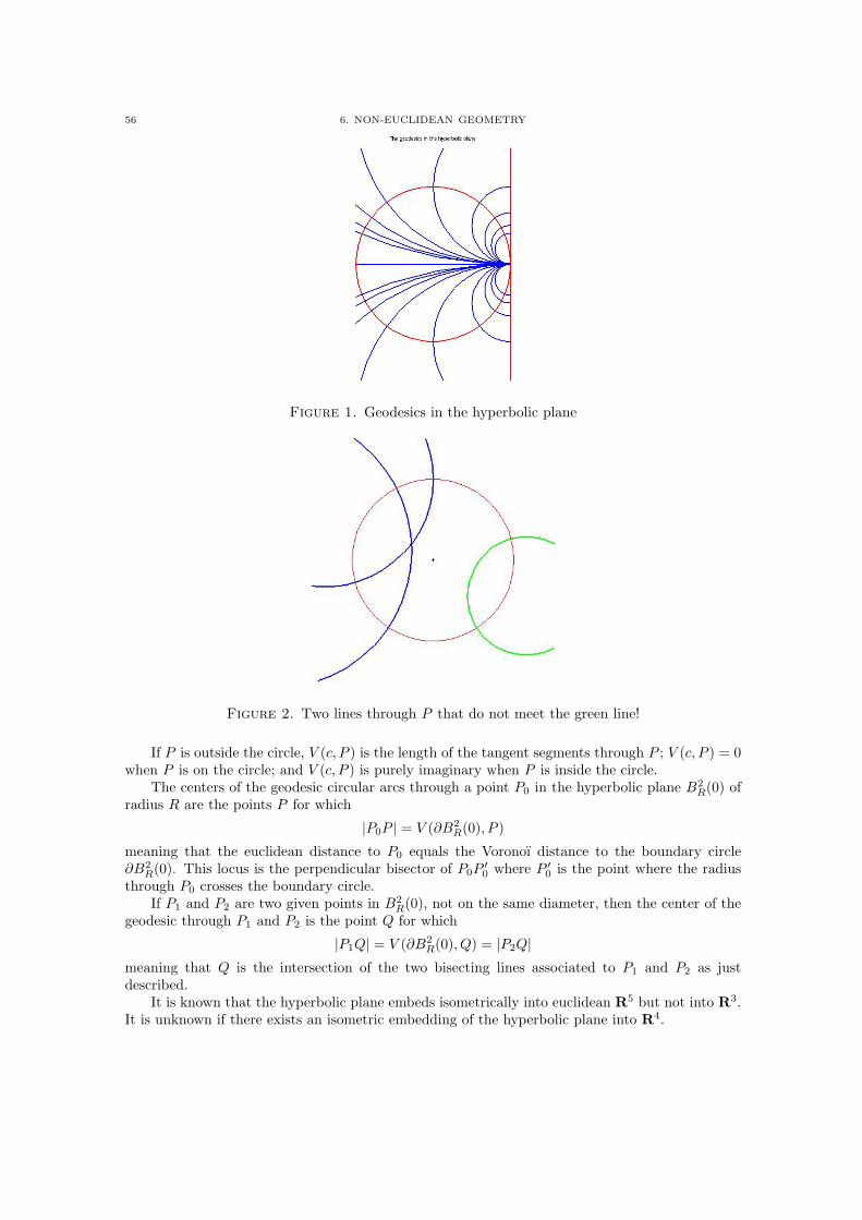
http://www-groups.dcs.st-and.ac.uk/history/HistTopics/Non-Euclidean_geometry.html

56 6. NON-EUCLIDEAN GEOMETRY

Figure 1. Geodesics in the hyperbolic plane

Figure 2. Two lines through P that do not meet the green line!

If P is outside the circle, V (c, P ) is the length of the tangent segments through P ; V (c, P ) = 0when P is on the circle; and V (c, P ) is purely imaginary when P is inside the circle.

The centers of the geodesic circular arcs through a point P0 in the hyperbolic plane B2R(0) of

radius R are the points P for which

|P0P | = V (∂B2R(0), P )

meaning that the euclidean distance to P0 equals the Voronoı distance to the boundary circle∂B2

R(0). This locus is the perpendicular bisector of P0P′0 where P ′0 is the point where the radius

through P0 crosses the boundary circle.If P1 and P2 are two given points in B2

R(0), not on the same diameter, then the center of thegeodesic through P1 and P2 is the point Q for which

|P1Q| = V (∂B2R(0), Q) = |P2Q|

meaning that Q is the intersection of the two bisecting lines associated to P1 and P2 as justdescribed.

It is known that the hyperbolic plane embeds isometrically into euclidean R5 but not into R3.It is unknown if there exists an isometric embedding of the hyperbolic plane into R4.

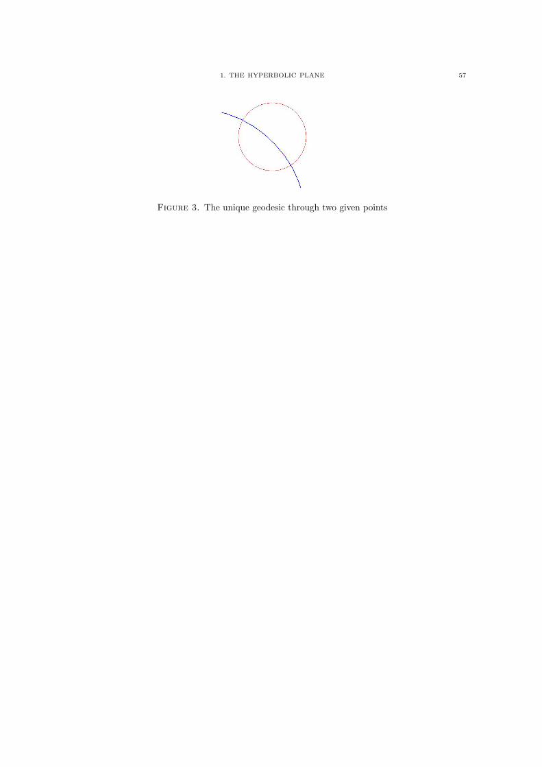
1. THE HYPERBOLIC PLANE 57

Figure 3. The unique geodesic through two given points

Bibliography

[1] Jeff Cheeger and David G. Ebin, Comparison theorems in Riemannian geometry, North-Holland Publishing Co.,Amsterdam, 1975, North-Holland Mathematical Library, Vol. 9. MR MR0458335 (56 #16538)

[2] G. S. Hall, Symmetries and curvature structure in general relativity, World Scientific Lecture Notes in Physics,vol. 46, World Scientific Publishing Co. Inc., River Edge, NJ, 2004. MR MR2109072

[3] S. W. Hawking and G. F. R. Ellis, The large scale structure of space-time, Cambridge University Press, London,

1973, Cambridge Monographs on Mathematical Physics, No. 1. MR MR0424186 (54 #12154)[4] John M. Lee, Riemannian manifolds, Graduate Texts in Mathematics, vol. 176, Springer-Verlag, New York,

1997, An introduction to curvature. MR MR1468735 (98d:53001)[5] Jesper M. Møller, General topology, http://www.math.ku.dk/~moller/e03/3gt/notes/gtnotes.pdf.[6] John Nash, The imbedding problem for Riemannian manifolds, Ann. of Math. (2) 63 (1956), 20–63. MR

MR0075639 (17,782b)[7] Barrett O’Neill, Semi-Riemannian geometry, Pure and Applied Mathematics, vol. 103, Academic Press Inc.

[Harcourt Brace Jovanovich Publishers], New York, 1983, With applications to relativity. MR MR719023(85f:53002)

[8] Michael Spivak, A comprehensive introduction to differential geometry. Vol. II, second ed., Publish or PerishInc., Wilmington, Del., 1979. MR MR532831 (82g:53003b)

59

http://www.math.ku.dk/~moller/e03/3gt/notes/gtnotes.pdf

Documents

Riemannian Geometry - kumoller/f05/genotes.pdf · Contents Chapter 1. Smooth manifolds 5 1. Tangent vectors, cotangent vectors and tensors 5 2. The tangent bundle of a smooth manifold