Riding the Yield Curve: A Variety of Strategies

Draft

6 RIDING THE YIELD CURVE: A VARIETY OF STRATEGIES SEPTEMBER 2005

In its simplest form, the rational expecta-tions hypothesis of the term structure ofinterest rates (REHTS) posits that in aworld with risk-neutral investors, the

n-period long rate is a weighted average of thefuture spot rates and thus any 1-period forwardrate is an unbiased predictor of the corre-sponding future 1-period spot rate. Conse-quently, the expectations hypothesis impliesthat with the possible exception of a term pre-mium, the holding period returns (HPRs) ofa class of fixed-income instruments are iden-tical, independent of the instruments’ originalmaturity.1 Under this assumption, for example,the returns from purchasing a 3-month gov-ernment security and holding it until maturityand the returns from purchasing a 12-monthgovernment security and holding it for 3months are identical. The strategy of pur-chasing a longer-dated security and selling itbefore maturity is referred to as “riding theyield curve.”

If the REHTS holds, then, for any givenholding period, riding strategies should notyield excess returns compared with holding ashort-dated security until maturity. Any evi-dence of persisting excess returns from suchtrading strategies would indicate the existenceof risk premia associated with the term struc-ture. The body of literature on different testsof the expectations hypothesis is very large,and overall the results remain inconclusive.2

Although the majority of tests of theexpectations hypothesis are hinged on testing

for the predictive power of forward rates interms of future sport rates, there is a smallstrand of literature that examines the persis-tence of excess returns from riding strategiesacross different holding horizons with differentmaturity instruments. In their seminal paper,Dyl and Joehnk [1981] examine differentriding strategies for U.S. T-bill issues from 1970to 1975 and find that there are significant,albeit small, excess HPRs to be made fromriding the yield curve. They use a simple filterrule based on break-even yield changes inorder to quantify the ex ante riskiness of ridingthe yield curve. Based on this filter, their resultsindicate that the returns increase with boththe holding horizon and the maturity of theinstrument.

Grieves and Marcus [1992] are able toproduce similar results by looking at a muchlonger time series of monthly zero-coupon T-bill rates from 1949 to 1988. They apply thesame filter rule as Dyl and Joehnk to identify,ex ante, under what type of yield curve envi-ronment excess returns from rolling can beanticipated. Although their results confirm thatlonger-maturity rides outperform the simplebuy-and-hold strategy of the short-terminstrument, they conclude that, on a risk-adjusted basis, longer rides perform slightlyworse because of increased interest rate risk.Overall, they find evidence against the pureform of the expectations hypothesis since itappears that profitable trading strategies havegone unexploited. Using daily closing prices

Riding the Yield Curve: A Variety of StrategiesDAVID S. BIERI AND LUDWIG B. CHINCARINI

DAVID S. BIERI

is adviser to the generalmanager at the Bank forInternational Settlementsin Basel, [email protected]

LUDWIG B.CHINCARINI

is an adjunct professor andfinancial consultant atGeorgetown University inWashington, [email protected]

Draft

for regular U.S. T-bill issues from 1987 to 1997, Grieveset al. [1999] are able to confirm these earlier findings, andthey also find that their results are relatively stable overtime. In contrast to Dyl and Joehnk, they conclude thatconditioning the ride on the steepness of the yield curvedoes not seem to improve the performance significantly.Most of the existing literature on excess returns fromriding the yield curve is exclusively limited to examiningthe money market sector of the yield curve, i.e. maturi-ties below 12 months, and has thus far only studied theU.S. Treasury market.3

In this article, we aim to add to this strand of liter-ature by looking at riding strategies for maturities beyondone year, looking at different currencies (euro and ster-ling), and also comparing rides between risk-free gov-ernment securities and instruments that contain somelevel of credit risk, namely, LIBOR-based deposits andswaps. In addition, we propose and test some forward-looking strategies based on either simple statistical mea-sures or economic models that incorporate the maindrivers of the yield curve. The main purpose of such rulesis to provide market practitioners with a simple tool setthat not only allows them to identify potentially prof-itable riding strategies but also enables an ex ante rankingof individual strategies.

RIDING THE YIELD CURVE

Riding the yield curve refers to the purchase of alonger-dated security and selling it before maturity.4 Thepurpose of riding the yield curve is to benefit from cer-tain interest rate environments. In particular, if a fixed-income manager has the choice between investing in a1-month deposit or a 12-month money market instrumentand selling after 1 month, there are certain rules of thumbas to which strategy might yield a higher return. Forinstance, when the yield curve is relatively steep andinterest rates are relatively stable, the manager will ben-efit by riding the curve rather than buying and holdingthe short-maturity instrument.

However, there are risks to riding the yield curve,most obviously the greater interest rate risk associated withthe riding strategy (as reflected by its higher duration).Thus, if one is riding and yields rise substantially, theinvestor will incur a capital loss on the riding position. Hadthe investor purchased the instrument that matched herinvestment horizon, she would have still ended up witha positive return.

REHTS AND RIDING THE YIELD CURVE

One implication of the REHTS is that with theexception of time-varying term premia, the return on alonger-period bond is identical to the return from rollingover a sequence of short-term bonds. As a consequence,longer-term rates yn

t are a weighted average of short-termrates ym

t plus the term premia. This can be expressed asfollows:

(1)

where ymt+h is the m-period zero-coupon yield at time t

+ h, Et is the conditional time expectations operator attime t, and σ n,m is the risk premium between n- and m-period zero-coupon bonds (with n > m). In Equation (1),k = n–m is restricted to be an integer.

In the absence of any risk premia, by taking expec-tations and subtracting ym

t from both sides we can rewriteEquation (1) as

(2)

Thus, under the REHTS, the future differentials onthe short rate are related to the current yield spreadbetween the long-term and short-term zero-coupon rates.Equation (2) forms the basis for most empirical tests ofthe REHTS, by running the regression

(3)

and testing whether β = 1. In practice, however, mostempirical studies report coefficients that are significantlydifferent from 1, which is almost exclusively taken as evi-dence for the existence of (time-varying) risk premia.5

Rather than postulating a linear relationship betweenthe future differentials on the short rate and the currentslope of the term structure as expressed in Equation (2),we calculate the ex post excess HPRs from riding theyield curve. Thus, if the REHTS holds and there are norisk premia, these returns should be zero.

Therefore, according to the REHTS, if all agentsare risk neutral and concerned only with the expectedreturn, the expected one-period HPR on all bonds, inde-

1

1

1

ky y y yt h

mtm

tn

tm

th

k

+=

−

− = + −( ) +∑ a b e

y yk

y ytn

tm

t hm

tm

h

k

− = −+=

−

∑1

1

1

yk

E ytn

t t hm n m

h

k

= ++=

−

∑1

0

1

s ,

SEPTEMBER 2005 THE JOURNAL OF FIXED INCOME 7

Draft

pendent of their maturity, should be identical and wouldbe equal to the return on a one-period asset:

(4)

where Hnt+1 denotes the HPR of an n-period instrument

between time t and t + 1. This result can now be used toderive the zero excess holding period return (XHPR)condition of the REHTS by restating equation (4) as

(5)

Hence, if the REHTS holds, we should not be ableto find any evidence that fixed-income managers are ableto obtain any significant non-zero XHPRs by riding theyield curve.

Mathematics of Riding

In this section, we derive the main mathematicalformulae for riding the yield curve relative to a buy-and-hold strategy. Because we evaluate different riding strate-gies for maturities beyond one year, we need to distinguishbetween riding a money-market instrument and riding abond-market instrument.

Furthermore, we are not only interested in evalu-ating riding returns for different maturities, but we alsoconsider the case where we use different instruments toride the yield curve. In particular, we consider the caseof comparing a ride using a (risk-free) government bondwith riding down the credit curve with a LIBOR/swap-based instrument. Because investors expect to be rewardedfor taking on non-diversifiable credit risk, two securitiesthat are identical except for the level of credit risk musthave different yields. Thus, comparing the returns fromtwo strategies that involve fixed-income instruments withdifferent credit risk would normally necessitate the spec-ification of a framework that deals appropriately withcredit risk.

However, drawing on results from the literature onthe determinants of swap spreads,6 we can assume thatthe yield differential between government securities andswaps is not primarily a consequence of their idiosyn-cratic credit risk. This strand of literature argues that evenin the absence of any credit or default risk, swap spreadswould be non-zero,7 since they predominantly dependon other factors such as

XH H ytn

tn

tm

+ += − =1 1 0

E H yt tn

tm

+ =1

• the yield differential between LIBOR rates and therepo rate for General Collateral

• the slope of the term structure of risk-free interest rates

• the relative supply of government corporate debt.

There are also other non-default factors, such as li-quidity and yield spread volatility, that may play an impor-tant role in determining yield spreads.8

In line with the pioneering work by Dyl and Joehnk[1981], we also derive a formula for quantifying the riskassociated with a given riding strategy. This measure istraditionally referred to as the “margin of safety” or“cushion” and can be used as a conditioning moment orfilter for different rides. By calculating the cushion of agiven riding strategy, the investor has an ex ante indica-tion of how much, ceteris paribus, interest rates would haveto have risen at the end of the holding period such thatany excess returns from riding would be eliminated. Thecushion is therefore also referred to as the “break-evenyield change.” We will also derive an approximate for-mula that may appeal to the market practitioner becauseof its simplicity and intuitive form.

Riding the money market curve. For the analysis ofriding the money market curve, we assume that our ratesare money-market or CD equivalent yields. We can pos-tulate that the price of an m-maturity money-marketinstrument at time t is given by

(6)

where ym,t represents the current CD equivalent yield9 ofthe instrument at time t, m is the number of days to theinstrument’s maturity, and z is the instrument and cur-rency-specific day count basis.10 We can also denote theprice of this same maturity instrument after a holdingperiod of h days as

(7)

where ym-h,t+h represents the interest rate valid for theinstrument, which has now m – h days left until finalredemption. Thus, the HPR of the ride of an m-matu-rity instrument between time t and time t + h is given by

P

ym h

z

m h t hM

m h t h

− +

− +

=

+( )

,

, ·-

100

1

P

ym

z

m tM

m t

,

, ·

=+

100

1


Draft

(8)

The XHPRs of this strategy of riding over the choiceof holding an instrument with the maturity equal to theinvestment horizon h can be expressed as

(9)

It follows from Equation (9) that riding the yieldcurve is more profitable, ceteris paribus, 1) the steeper theyield curve at the beginning of the ride (i.e., large valuesfor ym,t – yh,t) and 2) the lower the expected rate at theend of the holding period (i.e., ym-h,t+h is low).

Riding the bond curve. In line with the assumptionsfor computing the returns for money market instruments,the zero-coupon prices for maturities beyond one year,where our rates used are zero coupon yields, can be cal-culated. We can postulate that the price of an m-matu-rity zero-coupon bond at time t is given by

(10)

where ym,t represents the current zero-coupon yield ofthe instrument at time t, m is the instrument’s final matu-rity, and z is the appropriate day count basis. In line withEquation (7), we can denote the price of this same instru-ment after holding it for h days as

(11)

where ym-h,t+h represents the interest rate valid for thezero-coupon bond, which is now an m – h maturity instru-ment that was purchased h days ago. Following Equation(8), we can write the HPR from riding the zero couponbond curve as

(12)H

y

ym hB m t

m z

m h t h

m h z,,

/

,

/[ ]− +

−( )++( )

+( )−

1

11

Py

m h t hB

m h t h

m h z− +

− +−( )=

+( ),

,

/

100

1

Py

m tB

m t

m z,

,

/=

+( )( )100

1

XHy

m

z

ym h

z

m hM

m t

m h t h

[ , ]

,

,

=+

+ −

− +

1

1−−

−

1 y

h

zh t,

HP

P

ym

zm hM m h t h

M

m tM

m t

[ , ],

,

,

= − == ⋅

− + 1

1

11

1

+−( )

−

− +ym h

zm h t h, ·

Similarly, the excess holding returns from rollingdown the bond curve for h days are

(13)

It is important to reiterate at this point that Equa-tions (10)–(13) are expressed in terms of zero-couponrates; hence there are no coupon payments to be consid-ered. This does not mean, however, that our simple frame-work cannot be transposed to the (more realistic) worldof coupon-paying bonds. Using the approximation[(Pt+h)/Pt] – 1 ≈ ym,th/z – ∆yt Dt+h, we can restate Equa-tion (13) in a more applicable way:11

(14)

where ∆yt = ym-h,t+h – ym,t and Dm-h,t+h is the modifiedduration of the bond at the end of the holding horizon.By virtue of this approximation, the subsequent parts ofour analysis also apply to coupon-paying bonds.

Break-even rates and the cushion. Given a certainyield curve, the investor needs to decide whether to engagein a riding strategy before making an informed decisionabout selecting the appropriate instrument for the ride.The easiest way to make this decision is to use the cushionor break-even rate change as an indication of how muchrates would have to have increased at the end of theholding period h in order to make the riding returns equalto the returns from buying an h-maturity instrument andholding to maturity.

For example, if the yield curve is upward sloping,longer-term bonds offer a yield pick-up over the one-period short-term bonds. In order to equate the HPRsacross all bonds, the longer-maturity instruments wouldhave to incur a capital loss to offset their initial yield advan-tage. Break-even rates show by exactly how much long-term rates have to increase over the holding period tocause such capital losses. In other words, the break-evenrate is the implied end-horizon rate, y∗m–h,t, such thatthere are no excess returns from riding (i.e., XHt+h = 0).By setting XHm

[m,h] = 0 and XHB[m,h] = 0 in Equations (9)

XH

yh

zy D y

h

zm hB

m t t m h t h h t

,'

, , ,

[ ]

− +

≈−

−

D

<

−

−− +

if yearh

yh

zy Dm t t m h t h

1

, ,D 11 1 1+( ) −

>

y hh t

h z

,

/if year

XH

y

ym hB

m t

m z

m h t h

m h z

,

,

/

,

/

[ ]− +

−( )

=

+( )+( )

−

1

11

−

<yh

zhh t, if yea1 rr

1

11

+( )+( )

−

−− +

−( )y

y

m t

m z

m h t h

m h z

,

/

,

/11 1 1+( ) −

>

y hh t

h z

,

/if year


Draftand (13) respectively, we can derive the break-even ratesfor both cases:

Money markets ride:

(15)

Bond market ride:

(16)

We can now see that under the REHTS without anyterm premia, the break-even rate for a riding strategyusing an m-maturity instrument from time t to t + h isequivalent to the m – h period forward rate implied bythe term structure at time t (i.e., y∗m–h,t = fm–h,m). Thecushion can now be written as

y

y

yh

zm h t

m t

m z

h t− =

+( )+

,*

,

/

,

1

1

−

+( )+

−( )z m h

m t

m z

h

y

y

/

,

/

1

1

1

ifÄ Ä <Ä 1Ä year

hh t

h z

z m h

h

,

/

/

( )

−

−( )

1 ifÄ Ä >Ä 1Ä year

yy

m

zy

h

z

yh

z

zm h t

m t h t

h t

− =−

+

×,*

, ,

,1 mm h−

(17)

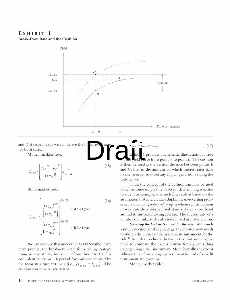
Exhibit 1 provides a schematic illustration of a rideon the yield curve from point A to point B. The cushionis then defined as the vertical distance between points Band C, that is, the amount by which interest rates haveto rise in order to offset any capital gains from riding theyield curve.

Thus, the concept of the cushion can now be usedto define some simple filter rules for determining whetherto ride. For example, one such filter rule is based on theassumption that interest rates display mean-reverting prop-erties and sends a positive riding signal whenever the cushionmoves outside a prespecified standard deviation bandaround its historic moving average. The success rate of anumber of similar such rules is discussed in a later section.

Selecting the best instrument for the ride. With sucha simple decision-making strategy, the investor now needsto address the choice of the appropriate instrument for theride.12 In order to choose between two instruments, weneed to compare the excess returns for a given ridingstrategy using either instrument. More formally, the excessriding returns from using a government instead of a creditinstrument are given by

Money market ride:

C y ym h m h t m h t[ , ]*

, ,= −− −


C

A

B

ym−h↪t

y∗m−h↪t

ym↪t

m − h m

Time to maturity

Cushion

Yield

E X H I B I T 1Break-Even Rate and the Cushion

Draft

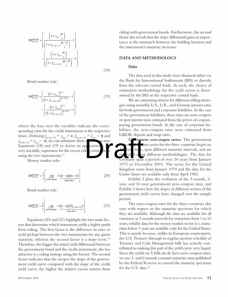
(18)

Bond market ride:

(19)

where the hats over the variables indicate the corre-sponding rates for the credit instrument at the respectivetimes. Defining ym-h,t+h = ym,t + ε, ym-h,t+h = ym,t – η andym-h,t+h = ym,t – c, we can substitute these conditions intoEquations (18) and (19) to derive an approximate, yetvery tractable, expression for the excess riding return fromusing the two instruments:13

Money market ride:

(20)

Bond market ride:

(21)

Equations (20) and (21) highlight the two main fac-tors that determine which instrument yields a higher profitfrom riding. The first factor is the difference in rates oryield pickup between the two instruments for any givenmaturity, whereas the second factor is a slope term.14

Therefore, the bigger the initial yield differential betweenthe government bond and the credit instrument, the lessattractive is a riding strategy using the former. The secondfactor indicates that the steeper the slope of the govern-ment yield curve compared with the slope of the credityield curve, the higher the relative excess returns from

XHz

h Dm h m[ , ]B,ride

initial spread

≈ − + −( ) −1

e c h{ hh t hz, +( )

slope effect

1 2444 3444

XHz

h m hm h[ , ]M,ride

initial spread

≈ − + −( ) −1e c h{ (( )

slope effect1 244 344

XHy

ym h

m t

m z

m h t h

m h[ , ],

/

,

( ) /B,ride =

+( )+( )− +

−

1

1zz

m t

m zy

−

−+( )

+

1

1

1

ˆ ,

/

ˆ ,

/ym h t h

m h z

− +−( )

−

1

XHy

m

z

ym h

z

m h

m t

m h t h

[ , ]

,

,

M,ride =+

+ −− +

1

1

−

−+

1

1 ˆ ,ym tt

m h t h

m

z

ym h

z

+ −

−

− +11

ˆ ,

riding with government bonds. Furthermore, the secondfactor also reveals that the slope differential gains in impor-tance as the mismatch between the holding horizon andthe instrument’s maturity increases.

DATA AND METHODOLOGY

Data

The data used in this study were obtained either viathe Bank for International Settlements (BIS) or directlyfrom the relevant central bank. As such, the choice ofestimation methodology for the yield curves is deter-mined by the BIS or the respective central bank.

We are estimating returns for different rolling strate-gies using monthly U.S., U.K., and German interest ratesfor both government and corporate liabilities. In the caseof the government liabilities, these rates are zero-couponor spot interest rates estimated from the prices of coupon-paying government bonds. In the case of corporate lia-bilities, the zero-coupon rates were estimated fromLIBOR deposit and swap rates.

Government zero-coupon curves. The governmentzero-coupon time series for the three countries begin ondifferent dates, span different maturity intervals, and areestimated using different methodologies. The data forGermany span a period of over 30 years from January1973 to December 2003. The series for the UnitedKingdom starts from January 1979 and the data for theUnites States are available only from April 1982.

Exhibit 2 plots the evolution of the 3-month, 2-year, and 10-year government zero-coupon rates, andExhibit 3 shows how the slopes of different sectors of thegovernment yield curves have changed over the sampleperiod.

The zero-coupon rates for the three countries alsovary with respect to the maturity spectrum for whichthey are available. Although the data are available for allcountries at 3-month intervals for maturities from 1 to 10years, reliable data for the money market sector (i.e. matu-rities below 1 year) are available only for the United States.This is mainly because, unlike its European counterparts,the U.S. Treasury through its regular auction schedule ofTreasury and Cash Management bills has actively con-tributed to making this part of the yield curve very liquid.Since the yields on T-bills are de facto zero-coupon rates,we use 3- and 6-month constant maturity rates publishedby the Federal Reserve to extend the maturity spectrumfor the U.S. data.15


DraftThe second column of Exhibit 2 shows the evolu-

tion of selected LIBOR/swap rates, and the changes inthe slopes of different sectors of the yield curve are dis-played in Exhibit 3. Exhibit 4 plots the development ofthe TED and swap spreads for the different currencies.The zero-coupon swap curves for each currency are esti-mated by the cubic B-splines method using LIBOR ratesup to 1 year and swap rates from 2 to 10 years.

Methodology

Zero-coupon curves are generally estimated fromobserved bond prices in order to obtain an undistortedestimate of a specific term structure. The approaches com-monly used to fit the term structure can broadly be sep-arated into two categories. On the one hand, parametriccurves are derived from interest rate models such as the


The majority of the central banks that report theirzero-coupon yield estimates to the BIS MEDTS, includingGermany’s Bundesbank, have adopted the so-calledNelson-Siegel approach [1987] or the Svensson [1994]extension thereof. Notable exceptions are the UnitedStates and the United Kingdom, both of which are usingspline-based methods to estimate zero-coupon rates.16

LIBOR/swap zero-coupon curves. The commercialbank liability zero-coupon rates are estimated fromLIBOR deposit and swap rates. Unlike the governmentdata, the series are computed using the same method-ology and span the same maturity spectrum, namely, 3months to 10 years at 3-monthly intervals. However, thestarting dates of the series vary by country. The data forthe United States are available from July 1987 to December2003, from August 1988 for Germany, and from January1990 for the United Kingdom.17

US

UK

Ger

Government LIBOR/SwapsY

ield

(%)

1982 1984 1986 1988 1990 1992 1994 1996 1998 2000 20020.0

2.5

5.0

7.5

10.0

12.5

15.03-month Bill

2-year Bond

10-year Bond

Yie

ld(%

)

1979 1981 1983 1985 1987 1989 1991 1993 1995 1997 1999 2001 20032

4

6

8

10

12

14

16

183-month Bill

2-year Bond

10-year Bond

Yie

ld(%

)

1973 1976 1979 1982 1985 1988 1991 1994 1997 2000 20032

4

6

8

10

12

1412-month Bill

2-year Bond

10-year Bond

Yie

ld(%

)

1987 1989 1991 1993 1995 1997 1999 2001 20030

2

4

6

8

10

123-month LIBOR

2-year Swap

10-year Swap

Yie

ld(%

)

1991 1992 1993 1994 1995 1996 1997 1998 1999 2000 2001 2002 20032

4

6

8

10

12

143-month LIBOR

2-year Swap

10-year Swap

Yie

ld(%

)

1988 1990 1992 1994 1996 1998 2000 20022

3

4

5

6

7

8

9

10

113-month LIBOR

2-year Swap

10-year Swap

E X H I B I T 2Evolution of Zero-Coupon Yield Curves with Shaded Recessions

DraftVasicek term structure model; on the other hand, non-parametric curves are curve-fitting models such as spline-based and Nelson-Siegel-type models.18 The two typesof non-parametric estimation techniques (Svensson andspline-based method) relevant for the data set used in thisarticle are described in more detail in Appendix 2.

PRACTICAL IMPLEMENTATION

Most empirical studies on the term structure ofinterest rates find that the data generally offer little sup-port for the REHTS. Our results are in line with thesefindings and suggest that market participants may be ableto exploit violations of the REHTS. Although there issome evidence that riding the yield curve per se may pro-duce excess returns compared with buying and holding,we suggest that using a variety of decision-making rules

could significantly increase the risk-adjusted returns ofvarious riding strategies. The relative merits of these deci-sion-making rules are evaluated by reporting the ex postexcess returns from riding down the yield curve, condi-tional on the rule sending a positive signal. Risk-adjustedexcess returns are expressed as Sharpe ratios in order tocompare and rank different riding strategies.

Before describing the individual decision-making rulesin more detail, we present a brief overview of the literaturedescribing the main factors that affect the yield curve.

Determinants of the Term Structure of Interest Rates

For many years, researchers in both macroeconomicsand finance have extensively studied the term structureof interest rates. Yet despite this common interest, the


US

UK

Ger

Government Slopes LIBOR/Swaps Slopes

Bas

isP

oin

ts

1982 1984 1986 1988 1990 1992 1994 1996 1998 2000 2002-100

-50

0

50

100

150

200

250

300

12-3 months

10-2 years

Bas

isP

oin

ts

1979 1981 1983 1985 1987 1989 1991 1993 1995 1997 1999 2001 2003-500

-400

-300

-200

-100

0

100

200

300

12-3 months

10-2 years

Bas

isP

oin

ts

1973 1976 1979 1982 1985 1988 1991 1994 1997 2000 2003-300

-200

-100

0

100

200

300

10-2 years

Bas

isP

oin

ts

1987 1989 1991 1993 1995 1997 1999 2001 2003-100

-50

0

50

100

150

200

250

300

350

12-3 months

10-2 years

Bas

isP

oin

ts

1991 1992 1993 1994 1995 1996 1997 1998 1999 2000 2001 2002 2003-150

-100

-50

0

50

100

150

200

250

300

12-3 months

10-2 years

Bas

isP

oin

ts

1988 1990 1992 1994 1996 1998 2000 2002-150

-100

-50

0

50

100

150

200

250

300

12-3 months

10-2 years

E X H I B I T 3Evolution of Zero-Coupon Yield Curve Slopes

Drafttwo disciplines remain remarkably far removed in theiranalysis of what makes the yield curve move. The buildingblocks of the dynamic asset-pricing approach in financeare affine models of latent (unobservable) factors with ano-arbitrage restriction. These models are purely statis-tical and provide very little in the way of explaining thenature and determination of these latent factors.19 Thefactors are commonly referred to as “level,’’ “slope,’’ and“curvature’’ (Litterman and Scheinkman [1991]) and awide range of empirical studies agree that almost all move-ments in the term structure of default-free interest ratesare captured by these three factors. In contrast, the macro-economic literature still relies on the expectations hypoth-esis of the term structure, despite overwhelming evidenceof variable term premia.

A handful of recent studies have started to connectthese two approaches by exploring the macroeconomic

determinants of the latent factors identified by empiricalstudies. In their pioneering work, Ang and Piazzesi [2003]develop a no-arbitrage model of the term structure thatincorporates measures of inflation and macroeconomicactivity in addition to the traditional latent factors—level,slope, and curvature. They find that including the twomacroeconomic factors improves the model’s ability toforecast the dynamics of the yield curve. Compared withtraditional latent factor models, the level factor remainsalmost unchanged when macro factors are incorporated,but a significant proportion of the slope and curvature fac-tors are attributed to the macro factors. However, theeffects are limited as the macro factors primarily explainmovements at the short end of the curve (in particularinflation), whereas the latent factors continue to accountfor most of the movement for medium to long maturities.20

Evans and Marshall [2002] analyze the same problem


12-Month TED Spreads

Bas

isP

oin

ts

1987 1988 1989 1990 1991 1992 1993 1994 1995 1996 1997 1998 1999 2000 2001 2002 2003-20

0

20

40

60

80

100

120

140

160USD RatesEUR RatesGBP Rates

10-Year Swap Spreads

Bas

isP

oin

ts

1987 1988 1989 1990 1991 1992 1993 1994 1995 1996 1997 1998 1999 2000 2001 2002 2003-50

0

50

100

150

200

250USD RatesEUR RatesGBP Rates

E X H I B I T 4Evolution of TED and Swap Spreads

Draft

using a different, VAR-based approach. They formulateseveral VARs and examine the impulses of the latent fac-tors to a broad range of macroeconomic shocks. Althoughthey confirm Ang and Piazzesi’s results that most of thevariability of short- and medium-term yields is driven bymacro factors, they also find that such observable factorsexplain much of the movement in long-term yields andthat they have a substantial and persistent impact on thelevel of the term structure.

Wu [2001, 2003] examines the empirical relation-ship between the slope factor of the term structure andexogenous monetary policy shocks in the United Statesafter 1982 in a VAR setting. He finds that there is a strongcorrelation between the slope factor and monetary policyshocks. In particular, his results indicate that such shocksexplain 80-90% of the variability of the slope factor.Although the influence is short lived, this provides strongevidence in support of the conjecture by Knez et al. [1994]on the relation between the slope factor and FederalReserve policy.21

Most recently, Rudebusch and Wu [2003] haveextended this research into the macroeconomic deter-minants of the yield curve by incorporating a latent factoraffine term structure model into an estimated structuralNew Keynesian model of inflation, the output gap, andthe federal funds rate. They find that the level factor ishighly correlated with long-run inflation expectationsand the slope factor is closely associated with changes ofthe federal funds rate.

Changes in the yield curve ultimately determine therelative success of riding the yield curve vis-à-vis buyingand holding. Any filter rule that aims to improve the per-formance of riding strategies must therefore somehow beconditioned on various (ex ante) measures of changes ofthe term structure of interest rates. In this context, we areexamining the performance of two broad categories of deci-sion-making rules, namely, statistical and macro-based rules.A given rule is said to send a positive signal if a certain triggerpoint has been reached by the observable variable(s), thebehavior of which is modeled by the rule.

Statistical Filter Rules

Statistical filters are a well-established relative valuetool among market practitioners. The main motivationfor using this type of rule is the belief that many financialvariables have mean-reverting properties, at least in theshort to medium term. In addition, such rules owe muchof their current popularity to the fact that they are easy to

implement and, with increasing access to real-time data,are often already implemented in many standard softwarepackages. We consider the following three simple rules.

Positive slope. In the simplest of all cases, assumingrelatively stable interest rates over the holding horizon,a positive slope is a sufficient condition for riding theyield curve. We define the slope of the term structure asthe yield differential between 10-year and 2-year ratesand implement a riding strategy whenever this slope isnon-zero.

Positive cushion. The cushion, or break-even ratechange, is a slightly more sophisticated measure of the rel-ative riskiness of a given riding strategy. As discussed above,the cushion indicates by how much interest rates have tochange over the holding horizon before the riding tradebegins to be unprofitable. A positive cushion indicates thatinterest rates have scope to increase without the trade incur-ring a negative excess return. With this filter rule, we imple-ment a riding strategy whenever the cushion is positive.

75%ile cushion. In most instances, the absolute basis-point size of the cushion will have an influence on theprofitability of the riding strategy, since for a given levelof interest rate volatility, a small positive cushion may notoffer sufficient protection compared with a large one.Assuming the cushion itself is normally distributed arounda zero mean, we compute the realized distribution of thecushion over a two-year interval prior to the date onwhich a riding trade is put on. A riding strategy is imple-mented whenever the cushion lies outside its two-yearmoving 75%ile.

Macro-Based Rules: Monetary Policy and Riding

In order to translate the link between the steepnessof the yield curve and monetary policy into potentiallyprofitable riding strategies, we need to formulate a tractablemodel of the interest rate policy followed by the centralbank, such as the Taylor rule.

The approach of a simple model of the FederalReserve’s behavior was first suggested by Mankiw andMiron [1986], who found that the REHTS was moreconsistent with data prior to the founding of the FederalReserve in 1913. This strand of literature argues that thereis a link between the Federal Reserve’s use of a fund ratetarget instrument and the apparent failure of the REHTS.22

Rather than developing an elaborate model of term premiacoupled with Federal Reserve behavior, our approachtakes the well-established Taylor rule (J. Taylor [1993]) as


Draft

a model for central bank behavior and tests for its predictivepower for excess returns by indicating changes in the slopeof the yield curve. In a second approach, we do not modelthe Federal Reserve’s behavior explicitly; instead, weextract the market’s expectations of future policy actionfrom the federal funds futures market. Before looking atthese more elaborate macro rules, we define a simple rulebased on a straightforward measure of economic activity.

The slope of the yield curve and recessions. Recessionsare often associated with a comparatively steep term struc-ture. As inflationary pressures are limited during such periodsof reduced economic activity, central banks are generallylowering their policy rates in order to stimulate the economy.

We define a riding strategy that engages in tradeswhenever the economy has entered into a recessionaryperiod. We use different definitions for recessions, depend-ing on the country in question. For the United States,recessions are defined according to the NBER’s BusinessCycle Dating Committee methodology, whereby “a reces-sion is a significant decline in economic activity spreadacross the economy, lasting more than a few months, nor-mally visible in real GDP, real income, employment, indus-trial production, and wholesale-retail sales.”23 For theUnited Kingdom and Germany, recessions are defined interms of at least two consecutive quarters during whichreal (seasonally adjusted) GDP is declining.

Using recessions as a trigger to ride the yield curve—while theoretically very appealing—suffers from a prac-tical drawback: agents do not know in real time when arecession begins and ends due to the reporting lag ofmacroeconomic data. This problem may be addressed by

conditioning the riding strategieson lagged “real-time” recessionsrather than “look-ahead” reces-sions.24

The slope of the yield curveand the Taylor rule. In this section,we examine how we can effectivelyemploy a simple Taylor rule to pre-dict future changes in the termstructure of interest rates fromchanges in the federal funds rate.As a first step, we verify that thereis a significant link between changesin the slope of the yield curve (i.e.,the degree by which the yieldcurve changes its slope over time)and changes in the short-terminterest rates, as suggested earlier.

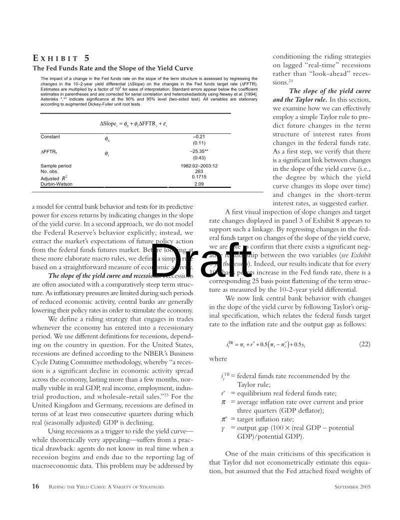
A first visual inspection of slope changes and targetrate changes displayed in panel 3 of Exhibit 8 appears tosupport such a linkage. By regressing changes in the fed-eral funds target on changes of the slope of the yield curve,we are able to confirm that there exists a significant neg-ative relationship between the two variables (see Exhibit5 for the results). Indeed, our results indicate that for every100 basis points increase in the Fed funds rate, there is acorresponding 25 basis point flattening of the term struc-ture as measured by the 10-2-year yield differential.

We now link central bank behavior with changesin the slope of the yield curve by following Taylor’s orig-inal specification, which relates the federal funds targetrate to the inflation rate and the output gap as follows:

(22)

where

itTR = federal funds rate recommended by the

Taylor rule; r∗ = equilibrium real federal funds rate; π = average inflation rate over current and prior

three quarters (GDP deflator); π∗ = target inflation rate;y = output gap (100 × (real GDP – potential

GDP)/potential GDP).

One of the main criticisms of this specification isthat Taylor did not econometrically estimate this equa-tion, but assumed that the Fed attached fixed weights of

i r yt t t t tTR = + + −( ) +p p p* *. .0 5 0 5


The impact of a change in the Fed funds rate on the slope of the term structure is assessed by regressing thechanges in the 10–2-year yield differential ( Slope) on the changes in the Fed funds target rate ( FFTR).Estimates are multiplied by a factor of 102 for ease of interpretation. Standard errors appear below the coefficientestimates in parentheses and are corrected for serial correlation and heteroskedasticity using Newey et al. [1994].Asterisks *,** indicate significance at the 90% and 95% level (two-sided test). All variables are stationaryaccording to augmented Dickey-Fuller unit root tests.

Slopet

=0

+1FFTR

t+

t

Constant0

–0.21(0.11)

FFTRt1

–25.35**(0.43)

Sample period 1982:02–2003:12No. obs. 263

Adjusted R2 0.1715

Durbin-Watson 2.09

E X H I B I T 5The Fed Funds Rate and the Slope of the Yield Curve

Draft

0.5 to deviations of both inflation and output.25 An addi-tional problem with Taylor’s original work is that theoutput gap is estimated in-sample. This shortcoming canbe addressed by estimating the Taylor rule out-of-samplewith no look-ahead bias (see panel 2 of Exhibit 6).26

As a response to the criticism that the weights oninflation and the output gap in Equation (22) are not esti-mated, we also consider a dynamic version of the TaylorRule, following the work of Judd and Rudebusch [1998].In this specification, Equation (22) is restated as an error-correction mechanism that allows for the possibility thatthe federal funds rate adjusts gradually to achieve the raterecommended by the rule. In particular, by adding a laggedoutput gap term along with the contemporaneous gap,Equation (22) is replaced with

(23)

The dynamics of adjustment of the actual level ofthe federal funds rate to the recommended rate, it

TR, aregiven by

(24)

This means that the change in the funds rate at timet partially corrects the difference between the last periodand the current target level as well as displaying somedependency on the funds rate change at time t – 1. Bysubstituting Equation (23) into Equation (24), we obtainthe full ECM to be estimated:

(25)

where α = r∗– λ1π∗. This equation provides estimates of

policy weights on inflation and output and on the speedof adjustment to the rule. Judging by the plot of our Judd-Rudebusch estimates of the Taylor rule alone (see panel 3of Exhibit 6), it is difficult to conclude whether we areable to obtain an improved forecast of the federal fundsrate, compared to the two static methods.

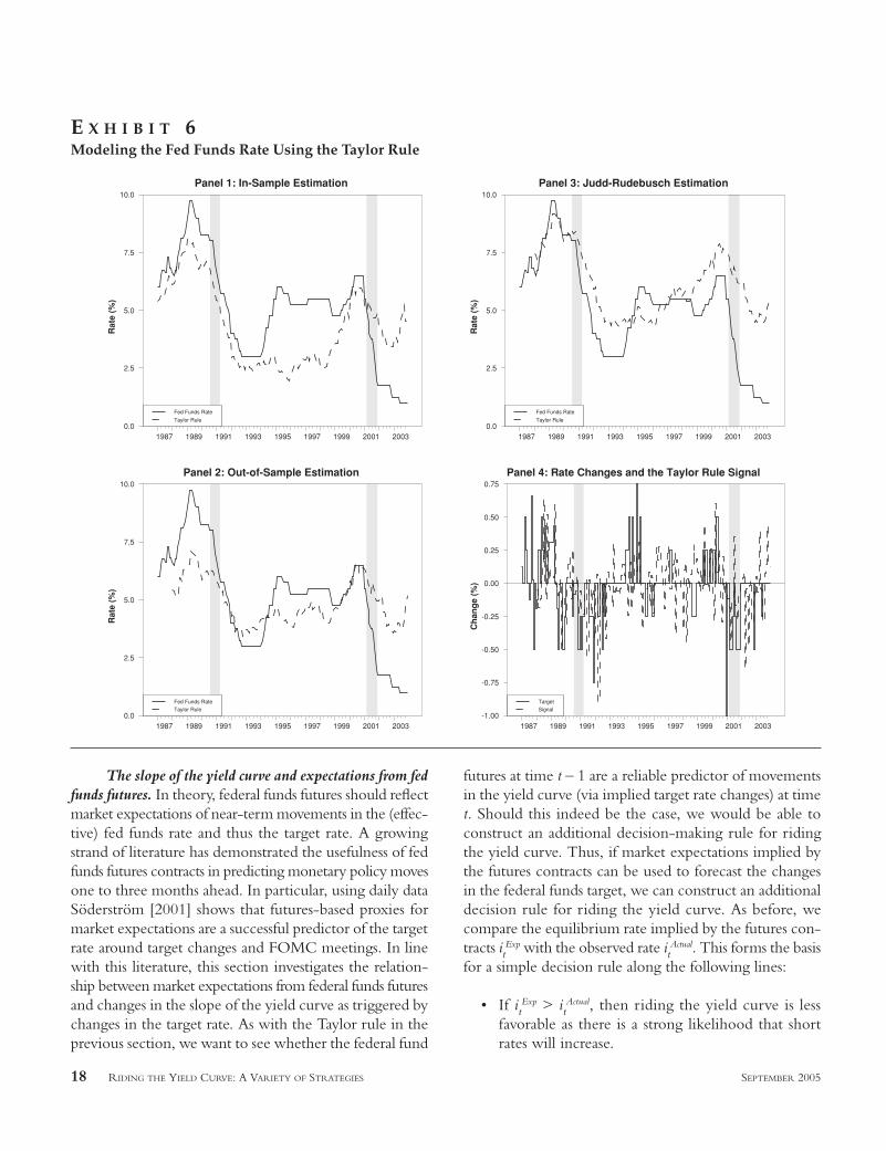
In order to determine whether the Taylor rule isa useful means for devising different riding strategies,we need to see whether the Taylor rule at time t – 1 canpredict changes in the federal funds rate at time t. If thisis indeed the case, we can use the Taylor rule as a signalto determine when to ride the yield curve, since wehave already established that the target rate can predictslope changes.

Rather than determination of the equilibrium level

D Di i y y it t t t t t= − + +( ) + + +− 1 3 − −ga g g l p gl gl r1 2 1 11

D Di i i it t t t= −( ) +− −g rTR1 1

π π λ π π λ λt t t t t tr y yTR = + + −( ) + +1 2 3 −* *

1

of the target rate, we are interested in predicting target ratechanges by employing the Taylor rule. For this purpose, weregress the actual changes in the federal funds target∆FFTRt on changes of the target rate, as recommendedby the Taylor rule ∆Taylort as opposed to the differencebetween the target rate estimate and the actual rate.27 Inorder to see whether the Taylor signal is particularly pre-dictive prior to an interest rate decision, we add a dummyvariable FOMCt that has a value only in the month priorto an FOMC meeting.

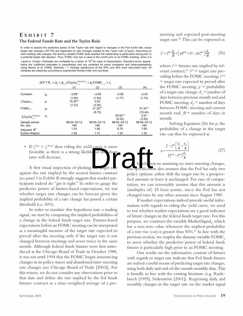
The results of these regressions are summarized inExhibit 7. For both versions of the Taylor rule (the out-of-sample estimation of the original specification and thedynamically estimated Judd-Rudebusch version), there isstrong significance on the predictive power of the Taylorrule with regards to target rate changes over the entiresample period (1988-2003).28 In addition, the respon-siveness of rate changes with respect to the Taylor ruleincreases by almost 20% before FOMC meetings. This isindicated by the increase in the parameter estimates ofregressions 2 and 4 in Exhibit 7. Nonetheless, the estimatesfor φ are significantly smaller than unity, suggesting thatthe recommended rate needs to change by between 120and 150 basis points to signal a full quarter percent changein the actual target rate.29

Having established a relatively firm link betweenthe Taylor rule and changes in the slope of the term struc-ture, we can devise a simple signal for whether to rideand compare it with alternative strategies. At every monthend, we estimate it

TR by re-estimating yt and πt. The changein the “equilibrium” federal funds target rate suggestedby the Taylor rule ∆it

TR is then used as the basis for asimple decision rule:

• If ∆itTR > 0, then riding the yield curve is less

favorable as there is a strong likelihood that shortrates will increase.

• If ∆itTR < 0 then riding the yield curve is more

favorable as there is a strong likelihood that shortrates will decrease.

In order to translate this decision-making rule intoa signal that indicates whether to ride the yield curve, weconstruct a variable TaylorSignalt that takes a value of 1(or –1) whenever the relevant specification of the Taylorrule indicates a rate rise (cut) and is 0 otherwise. Weemploy a riding strategy whenever the signal is differentfrom 1 and therefore does not indicate an impendingincrease in the target rate.


Draft

The slope of the yield curve and expectations from fedfunds futures. In theory, federal funds futures should reflectmarket expectations of near-term movements in the (effec-tive) fed funds rate and thus the target rate. A growingstrand of literature has demonstrated the usefulness of fedfunds futures contracts in predicting monetary policy movesone to three months ahead. In particular, using daily dataSöderström [2001] shows that futures-based proxies formarket expectations are a successful predictor of the targetrate around target changes and FOMC meetings. In linewith this literature, this section investigates the relation-ship between market expectations from federal funds futuresand changes in the slope of the yield curve as triggered bychanges in the target rate. As with the Taylor rule in theprevious section, we want to see whether the federal fund

futures at time t – 1 are a reliable predictor of movementsin the yield curve (via implied target rate changes) at timet. Should this indeed be the case, we would be able toconstruct an additional decision-making rule for ridingthe yield curve. Thus, if market expectations implied bythe futures contracts can be used to forecast the changesin the federal funds target, we can construct an additionaldecision rule for riding the yield curve. As before, wecompare the equilibrium rate implied by the futures con-tracts it

Exp with the observed rate itActual. This forms the basis

for a simple decision rule along the following lines:

• If itExp > it

Actual, then riding the yield curve is lessfavorable as there is a strong likelihood that shortrates will increase.


Panel 1: In-Sample Estimation

Rat

e(%

)

1987 1989 1991 1993 1995 1997 1999 2001 20030.0

2.5

5.0

7.5

10.0

Fed Funds Rate

Taylor Rule

Panel 2: Out-of-Sample Estimation

Rat

e(%

)

1987 1989 1991 1993 1995 1997 1999 2001 20030.0

2.5

5.0

7.5

10.0

Fed Funds RateTaylor Rule

Panel 3: Judd-Rudebusch Estimation

Rat

e(%

)

1987 1989 1991 1993 1995 1997 1999 2001 20030.0

2.5

5.0

7.5

10.0

Fed Funds Rate

Taylor Rule

Panel 4: Rate Changes and the Taylor Rule SignalC

han

ge

(%)

1987 1989 1991 1993 1995 1997 1999 2001 2003-1.00

-0.75

-0.50

-0.25

0.00

0.25

0.50

0.75

TargetSignal

E X H I B I T 6Modeling the Fed Funds Rate Using the Taylor Rule

Draft• If it

Exp < itActual then riding the yield curve is more

favorable as there is a strong likelihood that shortrates will decrease.

A first visual inspection of plotting the target rateagainst the rate implied by the nearest futures contract(see panel 1 in Exhibit 8) strongly suggests that market par-ticipants indeed do “get it right.” In order to gauge thepredictive power of futures-based expectations, we testwhether target rate changes can be forecast given theimplied probability of a rate change has passed a certainthreshold (i.e. 50%).

In order to translate this hypothesis into a tradingsignal, we start by computing the implied probabilities ofa change in the federal funds target rate. Futures-basedexpectations before an FOMC meeting can be interpretedas a meaningful measure of the target rate expected toprevail after the meeting only if the target rate is notchanged between meetings and never twice in the samemonth. Although federal funds futures were first intro-duced at the Chicago Board of Trade in October 1988,it was not until 1994 that the FOMC began announcingchanges in its policy stance and abandoned inter-meetingrate changes (see Chicago Board of Trade [2003]). Forthis reason, we do not consider any observations prior tothat date and define the rate implied by the fed fundsfutures contract as a time-weighted average of a pre-

meeting and expected post-meetingtarget rate.30 This can be expressed as

(26)

where i f = futures rate implied by rel-evant contract;31 i pre = target rate pre-vailing before the FOMC meeting; i post

= target rate expected to prevail afterthe FOMC meeting; p = probabilityof a target rate change; d1 = number ofdays between previous month end andFOMC meeting; d2 = number of daysbetween FOMC meeting and currentmonth end; B = number of days inmonth.

Solving Equation (26) for p, theprobability of a change in the targetrate can thus be expressed as

(27)

In addition to assuming no inter-meeting changes,this specification also assumes that the Fed has only twopolicy options: either shift the target rate by a prespeci-fied amount or leave it unchanged. For ease of compu-tation, we can reasonably assume that this amount is(multiples of ) 25 basis points, since the Fed has notchanged rates by any other amount since August 1989.

If market expectations indeed provide useful infor-mation with regards to riding the yield curve, we needto test whether market expectations are a good indicatorof future changes in the federal funds target rate. For thispurpose, we construct the variable MarketSignalt, whichhas a non-zero value whenever the implied probabilityof a rate rise (cut) is greater than 50%.31 In line with theprevious section, we employ the dummy variable FOMCtto assess whether the predictive power of federal fundsfutures is particularly high prior to an FOMC meeting.

Our results on the informative content of futureswith regards to target rate indicate that Fed funds futuresare indeed a useful means of predicting target rate changes,using both daily and end-of-the-month monthly data. Thisis broadly in line with the existing literature (e.g. Rude-busch [1995]; Söderström [2001]). Regressing daily andmonthly changes in the target rate on the market signal

p

i id

B

d

B

i id

B

t t

t t

=− +

−( )

f pre

post pre

1 2

2

i id

Bpi p i

d

Bt i t if pre post pre= + + −( )

1 21


In order to assess the predictive power of the Taylor rule with regard to changes in the Fed funds rate, actualtarget rate changes ( FFTR) are regressed on rate changes implied by the Taylor rule ( Taylor). Assuming nointer-meeting rate changes, the dummy variable FOMC tests whether the relationship is particularly strong prior toa potential target rate decision. Thus, FOMC only has a value in the month prior to an FOMC meeting, when it is

equal to Taylor. Estimates are multiplied by a factor of 102 for ease of interpretation. Standard errors appearbelow the coefficient estimates in parentheses and are corrected for serial correlation and heteroskedasticityusing Newey et al. [1994]. Asterisks *,** indicate significance at the 90% and 95% level (two-sided test). Allvariables are stationary according to augmented Dickey-Fuller unit root tests.

FFTRt

= 0 + 1,3 aylort 1(Dynamic) + 2FO C

t 1 +t

(1) (2) (3) (4)

Constant 0 –2.98* –2.99 –2.56 –2.50(1.84) (1.83) (1.77) (1.74)

Taylort-1 1 15.39** 0.02(7.23) (2.05)

FOMCt-1 2 21.29** 31.34**(9.79) (10.44)

Taylort 1Dynamic 3 28.92**

(8.32)2.67

(3.83)Sample period 88:04–03:12 88:04–03:12 88:04–03:12 88:04–03:12No. obs. 189 189 190 190

Adjusted R2 1.53 1.80 6.79 7.68

Durbin-Watson 1.29 1.31 1.34 1.35

E X H I B I T 7The Federal Funds Rate and the Taylor Rule

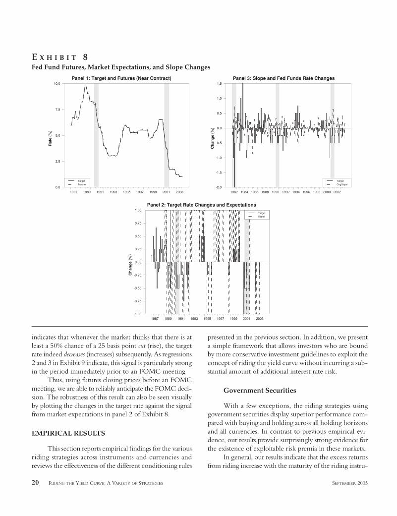
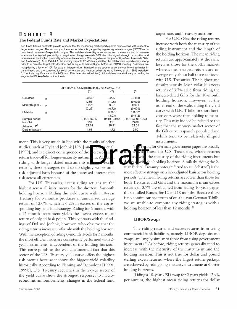
Draftindicates that whenever the market thinks that there is atleast a 50% chance of a 25 basis point cut (rise), the targetrate indeed decreases (increases) subsequently. As regressions2 and 3 in Exhibit 9 indicate, this signal is particularly strongin the period immediately prior to an FOMC meeting

Thus, using futures closing prices before an FOMCmeeting, we are able to reliably anticipate the FOMC deci-sion. The robustness of this result can also be seen visuallyby plotting the changes in the target rate against the signalfrom market expectations in panel 2 of Exhibit 8.

EMPIRICAL RESULTS

This section reports empirical findings for the variousriding strategies across instruments and currencies andreviews the effectiveness of the different conditioning rules

presented in the previous section. In addition, we presenta simple framework that allows investors who are boundby more conservative investment guidelines to exploit theconcept of riding the yield curve without incurring a sub-stantial amount of additional interest rate risk.

Government Securities

With a few exceptions, the riding strategies usinggovernment securities display superior performance com-pared with buying and holding across all holding horizonsand all currencies. In contrast to previous empirical evi-dence, our results provide surprisingly strong evidence forthe existence of exploitable risk premia in these markets.

In general, our results indicate that the excess returnsfrom riding increase with the maturity of the riding instru-


Panel 1: Target and Futures (Near Contract)

Rat

e(%

)

1987 1989 1991 1993 1995 1997 1999 2001 20030.0

2.5

5.0

7.5

10.0

Target

Futures

Panel 2: Target Rate Changes and Expectations

Ch

ang

e(%

)

1987 1989 1991 1993 1995 1997 1999 2001 2003-1.00

-0.75

-0.50

-0.25

0.00

0.25

0.50

0.75

1.00TargetSignal

Panel 3: Slope and Fed Funds Rate Changes

Ch

ang

e(%

)

1982 1984 1986 1988 1990 1992 1994 1996 1998 2000 2002-2.0

-1.5

-1.0

-0.5

0.0

0.5

1.0

1.5

Target

ChgSlope

E X H I B I T 8Fed Fund Futures, Market Expectations, and Slope Changes

Draftment. This is very much in line with the results of otherstudies, such as Dyl and Joehnk [1981] and Grieves et al.[1999], and is a direct consequence of the increased risk-return trade-off for longer-maturity instruments. Althoughriding with longer-dated instruments increases excessreturns, these strategies tend to do slightly worse on arisk-adjusted basis because of the increased interest raterisk across all currencies.

For U.S. Treasuries, excess riding returns are thehighest across all instruments for the shortest, 3-monthholding horizon. Riding the yield curve with a 10-yearTreasury for 3 months produces an annualized averagereturn of 12.0%, which is 6.2% in excess of the corre-sponding buy-and-hold strategy. Riding for 6 months witha 12-month instrument yields the lowest excess meanreturn of only 44 basis points. This contrasts with the find-ings of Dyl and Joehnk, however, who observe that theriding returns increase uniformly with the holding horizon.With the exception of riding 6-month T-bills for 3 months,the most efficient rides are consistently performed with 2-year instruments, independent of the holding horizon.This corresponds to the well-documented fact that thissector of the U.S. Treasury yield curve offers the highestrisk premia because it shows the biggest yield volatilityhistorically. According to Fleming and Remolona [1999a,1999b], U.S. Treasury securities in the 2-year sector ofthe yield curve show the strongest responses to macro-economic announcements, changes in the federal fund

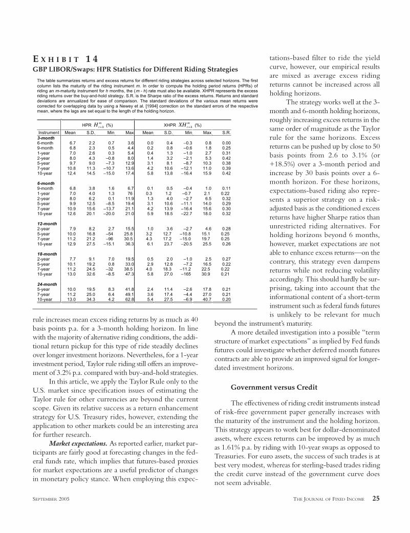
target rate, and Treasury auctions.For U.K. Gilts, the riding returns

increase with both the maturity of theriding instrument and the length ofthe holding horizon. The mean ridingreturns are approximately at the samelevels as those for the dollar market,whereas mean excess returns are onaverage only about half those achievedwith U.S. Treasuries. The highest andsimultaneously least volatile excessreturns of 3.7% arise from riding thelongest-dated Gilts for the 18-monthholding horizon. However, at theother end of the scale, riding the yieldcurve with U.K. T-bills for short hori-zons does worse than holding to matu-rity. This may indeed be related to thefact that the money-market sector ofthe Gilt curve is sparsely populated andT-bills tend to be relatively illiquidinstruments.

The results for German government paper are broadlyin line with those for U.S. Treasuries, where returnsincrease with the maturity of the riding instruments butdecrease with the holding horizon. Similarly, riding the 2-year Federal Treasury notes (referred to as “Schätze”) is themost effective strategy on a risk-adjusted basis across holdingperiods. The mean riding returns are lower than those forboth Treasuries and Gilts and the maximum mean excessreturns of 3.7% are obtained from riding 10-year paper,the so-called Bunds, for 12 and 18 months. Because thereis no continuous spectrum of on-the-run German T-bills,we are unable to compute any riding strategies with aholding horizon of less than 12 months.32

LIBOR/Swaps

The riding returns and excess returns from usingcommercial bank liabilities, namely, LIBOR deposits andswaps, are largely similar to those from using governmentinstruments.33 As before, riding returns generally tend toincrease with the maturity of the instrument and theholding horizon. This is not true for dollar and poundsterling excess returns, where the largest return pickupsare achieved by riding long-maturity instruments at shorterholding horizons.

Riding a 10-year USD swap for 2 years yields 12.9%per annum, the highest mean riding returns for dollar


Fed funds futures contracts provide a useful tool for measuring market participants’ expectations with respect totarget rate changes. The accuracy of these expectations is gauged by regressing actual changes ( FFTR) on aconditional measure of expected changes. The variable MarketSignal serves as such a measure and is non-zerowhenever the implied probability a target rate change exceeds 50% (i.e., the signal strength is positive andincreases as the implied probability of a rate rise exceeds 50%; negative as the probability of a cut exceeds 50%;and 0 otherwise). As in Exhibit 7, the dummy variable FOMC tests whether the relationship is particularly strongprior to a potential target rate decision and is equal to MarketSignal before an FOMC meeting. Estimates aremultiplied by a factor of 102 for ease of interpretation. Standard errors appear below the coefficient estimates inparentheses and are corrected for serial correlation and heteroskedasticity using Newey et al. [1994]. Asterisks*,** indicate significance at the 90% and 95% level (two-sided test). All variables are stationary according toaugmented Dickey-Fuller unit root tests.

FFTRt = 0 + 1 MarketSignalt-1 + 2 FOMCt-1 + t

(1) (2) (3)

Constant 0 –3.66* –2.87 –0.030(2.01) (1.96) (0.076)

MarketSignalt-1 1 8.99** 0.97 0.001(2.25) (0.72) (0.000)

FOMCt-1 2 10.90** 1.981**(3.03) (0.812)

Sample period 94:01–03:12 94:01–03:12 94:01:03–03:12:31No. obs. 116 116 2480

Adjusted R2 21.01 26.91 21.51

Durbin-Watson 1.81 1.72 2.00

E X H I B I T 9The Federal Funds Rate and Market Expectations

Draftinstruments. This is a mere 70 basis points more than thesame riding strategy using Treasuries instead. The highestexcess returns (6.6% p.a.) are obtained by riding the samematurity instrument, but over only a 3-month horizon.As with Treasuries, shorter holding horizons perform beston a risk-adjusted basis, and the 2-year maturity bucketoffers the most attractive reward-to-variability ratios. Thestrategy of riding a 2-year dollar swap for 3 months has aSharpe ratio of 0.54, the highest ratio across all creditstrategies. Riding only 6-month U.S. T-bills over the samehorizon offers a superior risk-adjusted profit with a Sharperatio of 0.71.

Sterling mean riding returns are consistently higherthan the ones for U.S. dollars and peak at 13.0% forriding a 10-year swap for both 18 months and 2 years.Mean excess returns are at similar levels as the ones indollars, albeit marginally more volatile, which stands instark contrast to riding government instruments, wheresterling excess returns were only half the size of dollarreturns. Riding the yield curve with short-maturity

instruments for short holding hori-zons is the least attractive strategy,with riding a 6-month deposit for 3months offering no excess returns.Unlike for government paper, how-ever, none of the riding strategies doesworse than the corresponding buy-and-hold investment.

This is not the case for strategieswith euro-denominated deposits,where money-market rides over a 3-month period either offer no returnenhancement or do worse thanmatching maturity and investmenthorizon. In addition, euro credit ridesshow slightly lower mean returns thangovernment rides (10.1% versus 10.0%for riding the respective 10-year instru-ment for 2 years), whereas mean excessreturns are on average only marginallyhigher than for the risk-free rides. Thisfollows directly from the historicalbehavior of euro deposit and swapspreads, which display high levels ofvolatility throughout the entire sampleperiod, despite their very low levels.Despite the fact that the euro swapsmarket has a higher notional amountoutstanding than any other currency,34

the absence of any significant swap spreads suggests thateurozone credit is more expensive than credit elsewhere.This phenomenon, sometimes referred to as the “eurocredit puzzle,” is illustrated in Exhibit 4.

Conditioned Riding

This section reports the results from applying avariety of statistical and macro-based decision-makingrules to the different riding strategies. Overall we findstrong evidence that the excess returns of a large numberof riding strategies can be enhanced significantly by relyingon these rules. This in itself points to the existence of siz-able risk premia that can be exploited successfully.

Positive slope. This simplest of ex ante filteringmechanism produces mixed results at improving meanexcess riding returns across most of the instruments,holding horizons, and currencies. Generally, the amountby which the excess returns rise tends to be highest forthe shortest available holding horizons.


The table summarizes returns and excess returns for different riding strategies across selected horizons. The firstcolumn lists the maturity of the riding instrument m. In order to compute the holding period returns (HPRs) ofriding an m-maturity instrument for h months, the (m - h) rate must also be available. XHPR represents the excessriding returns over the buy-and-hold strategy. S.R. is the Sharpe ratio of the excess returns. Returns and standarddeviations are annualized for ease of comparison. The standard deviations of the various mean returns werecorrected for overlapping data by using a Newey et al. [1994] correction on the standard errors of the respectivemean, where the lags are set equal to the length of the holding horizon.

HPR Ht +hm

(%) XHPR XHt +hm

(%)

Instrument Mean S.D. Min Max Mean S.D. Min Max S.R.3-month6-month 6.3 2.8 0.3 5.0 0.5 0.7 –0.3 1.7 0.712-year 7.8 4.9 –1.5 8.4 2.0 3.9 –2.5 5.2 0.525-year 9.8 10.1 –5.5 14.8 4.0 9.5 –7.0 12.1 0.427-year 10.8 13.2 –7.6 20.0 5.0 12.7 –10.0 17.4 0.3910-year 12.0 17.9 –116 27.4 6.2 17.4 –13.9 24.7 0.35

6-month1-year 6.5 5.1 0.6 9.3 0.4 1.6 –1.1 2.3 0.282-year 7.7 7.4 –0.3 13.9 1.7 4.8 –2.4 6.8 0.355-year 9.9 14.3 –4.7 24.4 3.8 12.7 –7.8 17.3 0.307-year 10.9 18.5 –8.1 29.5 4.8 17.1 –11.3 22.4 0.2810-year 12.1 25.1 –12.7 37.6 6.0 23.8 –175 31.0 0.25

12-month2-year 7.6 10.4 1.2 18.7 1.2 4.7 –2.4 56 0.255-year 9.9 18.9 –4.2 29.5 3.5 15.7 –8.9 17.8 0.227-year 10.9 24.9 –7.2 39.6 4.5 22.2 –14.1 30.1 0.2010-year 12.2 33.4 –13.3 54.4 5.8 31.3 –224 45.0 0.18

18-month2-year 7.4 12.5 4.4 23.7 0.5 2.8 –1.1 3.10 0.195-year 9.8 22.0 –1.2 40.9 3.0 16.0 –8.5 22.1 0.197-year 10.9 28.5 –3.5 52.2 4.1 23.3 –14.9 35.4 0.1810-year 12.2 37.3 –108 69.7 5.4 33.0 –24.7 51.8 0.16

24-month5-year 9.8 25.3 4.4 51.1 2.6 15.0 –6.6 24.6 0.177-year 10.9 31.8 1.6 67.1 3.7 22.3 –9.6 40.6 0.1710-year 12.2 40.1 –1.9 95.3 5.0 31.5 –12.0 68.9 0.16

E X H I B I T 1 0U.S. Treasuries: HPR Statistics for Different Riding Strategies

Draft

For rides with either U.S. Trea-suries or German Bunds, a positiveslope is not able to improve the excessreturns at any horizon. This is in linewith the results of Grieves et al. [1992],whose study covers a similar sampleperiod but uses daily data. For mostother instruments, there are significantexcess returns at short horizons, butexcess returns fall below the uncondi-tioned riding returns for holdinghorizons beyond 1 year. Using dollar-denominated deposits and swaps, forexample, the mean excess returns areimproved by over 60 basis points, from4.04 to 4.68% p.a. for 3-month rides.For any longer horizon, however, theunconditioned returns are higher.

Euro-deposits perform even bet-ter, with mean excess returns improv-ing by over 350 basis points for3-month rides and over 30 basis pointsfor 2-year rides. Conditioned rideswith sterling instruments also producehigher mean excess returns for holdinghorizons up to 1 year.

Positive and 75%ile cushion. Inquantifying how much rates have toincrease before a riding trade losesmoney, it comes as no surprise thatusing the cushion as a filter performsbetter than just looking at the slope.For all rides except the percentilecushion in the case of sterling creditinstruments, both cushion-based con-ditions increase mean excess returnssignificantly.

In fact, of all the filtering strate-gies presented in this article, the per-centile cushion is by far the mosteffective method to enhance ridingreturns across all instruments and cur-rencies. This is again a fairly intuitive,yet powerful, result that states that thehigher the break-even interest ratechange at the beginning of the ridingperiod, the more profitable it is to ride.The biggest increases are obtainedwith dollar-based instruments, where



HPR Ht +hm

(%) XHPR XHt +hm

(%)

Instrument Mean S.D. Min Max Mean S.D. Min Max S.R.3-month6-month 5.6 1.4 0.7 3.1 –0.1 0.3 –0.2 0.2 –0.299-month 7.8 2.9 0.4 4.2 –0.2 0.7 –0.8 05 –0.281-year 8.0 3.1 0.1 4.8 –0.2 1.1 –1.1 0.8 –0.192-year 8.9 5.1 –1.1 7.6 0.2 2.4 –2.3 2.0 0.105-year 10.2 11.4 –8.9 17.0 0.9 6.3 –6.7 4.7 0.147-year 10.9 14.4 –11.6 20.3 1.4 8.2 –8.7 6.0 0.1710-year 11.8 18.1 –139 28.4 2.3 10.6 –10.6 7.8 0.22

6-month9-month 5.9 2.5 1.5 7.0 –0.1 0.5 –0.7 0.3 –0.211-year 8.0 4.8 1.2 81 –0.4 1.7 –2.4 1.8 –0.222-year 9.0 7.2 0.1 12.0 0.2 4.5 –4.9 6.1 0.045-year 10.3 15.0 –8.3 23.8 1.3 12.7 –13.8 17.4 0.107-year 11.0 18.7 –12.4 29.5 1.9 16.3 –17.0 20.1 0.1210-year 11.8 23.0 –172 41.8 2.6 20.3 –21.7 21.2 0.13

12-month2-year 9.2 10.8 3.0 21.3 0.5 4.8 –4.2 6.8 0.115-year 10.6 18.8 –4.6 42.8 1.9 15.6 –13.8 28.3 0.127-year 11.4 23.6 –8.4 52.4 2.8 21.0 –17.7 37.9 0.1310-year 12.3 30.6 –128 64.2 3.6 28.9 –23.7 49.7 0.13

18-month2-year 9.0 13.7 6.3 25.6 0.2 2.7 –2.8 3.1 0.095-year 10.8 21.8 0.9 44.9 1.8 15.2 –12.8 22.6 0.127-year 11.7 27.4 –2.6 53.2 2.7 21.9 –18.1 30.8 0.1210-year 12.7 36.1 –103 67.6 3.7 32.4 –25.8 44.6 0.11

24-month5-year 11.0 25.4 5.5 52.5 1.6 14.2 –12.3 21.1 0.117-year 11.9 31.3 1.0 63.0 2.6 21.7 –18.4 31.7 0.1210-year 13.0 40.7 –5.2 79.8 3.6 33.6 –276 47.8 0.11

E X H I B I T 1 1U.K. Gilts: HPR Statistics for Different Riding Strategies


HPR Ht +hm

(%) XHPR XHt +hm

(%)

Instrument Mean S.D Min Max Mean S.D. Min Max S.R.12-month2-year 6.7 9.6 0.9 16.0 0.8 5.1 –5.2 5.4 0.155-year 8.3 17.7 –5.9 23.0 2.4 16.0 –14.0 14.3 0.157-year 8.9 22.5 –9.6 26.6 3.0 21.4 –17.7 18.8 0.1410-year 9.6 29.0 –11.9 37.1 3.7 28.5 –20.0 27.8 0.13

18-month5-year 8.4 22.0 –4.0 34.3 2.2 18.0 –13.6 15.2 0.127-year 9.1 27.7 –9.0 37.4 2.9 24.8 –18.1 23.1 0.1210-year 9.9 35.3 –15.6 46.8 3.7 33.4 –22.7 33.0 0.11

24-month5-year 8.5 25.4 –3.3 36.7 2.0 18.5 –13.4 14.9 0.117-year 9.2 32.1 –8.9 40.3 2.7 26.8 –19.3 23.5 0.1010-year 10.1 41.1 –151 52.4 3.6 37.2 –23.6 35.4 0.10

E X H I B I T 1 2German Government Bonds: HPR Statistics for Different Riding Strategies

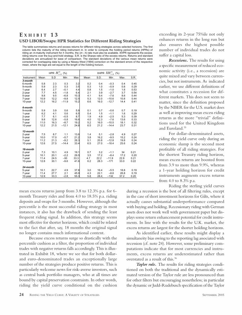
Draftmean excess returns jump from 3.8 to 12.3% p.a. for 6-month Treasury rides and from 4.0 to 18.5% p.a. ridingdeposits and swaps for 3 months. However, although thepercentile is the most successful riding strategy in mostinstances, it also has the drawback of sending the leastfrequent riding signal. In addition, this strategy seemsmost effective for shorter horizons, which could be relatedto the fact that after, say, 18 months the original signalno longer contains much informational content.

Because excess returns surge so drastically with thepercentile cushion as a filter, the proportion of individualtrades with negative returns falls accordingly. This is illus-trated in Exhibit 18, where we see that for both dollar-and euro-denominated trades an exceptionally largenumber of the strategies produce positive returns. This isparticularly welcome news for risk-averse investors, suchas central bank portfolio managers, who at all times arebound by capital preservation constraints. In other words,riding the yield curve conditional on the cushion

exceeding its 2-year 75%ile not onlyenhances returns in the long run butalso ensures the highest possiblenumber of individual trades do notsuffer a capital loss.

Recessions. The results for usinga specific measurement of reduced eco-nomic activity (i.e., a recession) arequite mixed and vary between curren-cies, but not instruments. As indicatedearlier, we use different definitions ofwhat constitutes a recession for dif-ferent markets. This does not seem tomatter, since the definition proposedby the NBER for the U.S. market doesas well at improving mean excess ridingreturns as the more “trivial” defini-tions used for the United Kingdomand Euroland.35

For dollar-denominated assets,riding the yield curve only during aneconomic slump is the second mostprofitable of all riding strategies. Forthe shortest Treasury riding horizon,mean excess returns are boosted fromfrom 3.9 to more than 9.9%, whereasa 1-year holding horizon for creditinstruments augments excess returnsfrom 4.0 to 8.3% p.a.

Riding the sterling yield curvesduring a recession is the best of all filtering rules, exceptin the case of short investment horizons for Gilts, where itactually causes substantial underperformance comparedwith buying and holding. Recessionary riding with Germanassets does not work well with government paper but dis-plays some return enhancement potential for credit instru-ments. In line with the results for the U.K. market, theexcess returns are largest for the shorter holding horizons.

As identified earlier, these results might display asimultaneity bias owing to the reporting lag associated withrecession (cf. note 24). However, some preliminary com-putations indicate that for most currencies and instru-ments, excess returns are underestimated rather thanoverstated as a result of this.36

Taylor rule. The results for riding strategies condi-tioned on both the traditional and the dynamically esti-mated version of the Taylor rule are less pronounced thanfor other filters but encouraging nonetheless; in particularthe dynamic or Judd-Rudebusch specification of the Taylor


The table summarizes returns and excess returns for different riding strategies across selected horizons. The firstcolumn lists the maturity of the riding instrument m. In order to compute the holding period returns (HPRs) ofriding an m-maturity instrument for h months, the (m - h) rate must also be available. XHPR represents the excessriding returns over the buy-and-hold strategy. S.R. is the Sharpe ratio of the excess returns. Returns and standarddeviations are annualized for ease of comparison. The standard deviations of the various mean returns werecorrected for overlapping data by using a Newey-West [1994] correction on the standard errors of the respectivemean, where the lags are set equal to the length of the holding horizon.

HPR Ht +hm

(%) XHPR XHt +hm

(%)

Instrument Mean S.D Min Max Mean S.D. Min Max S.R.3-month6-month 5.8 2.3 0.3 3.2 0.2 0.4 –0.3 0.4 0.459-month 5.9 2.3 0.3 3.5 0.3 1.0 –0.9 0.8 0.291-year 6.4 2.7 –0.1 4.4 0.8 1.5 –1.0 1.6 0.532-year 7.7 4.5 –1.8 6.4 2.1 3.9 –2.7 3.7 0.545-year 9.8 9.5 –6.8 10.3 4.1 9.4 –7.6 8.6 0.447-year 10.9 12.2 –9.8 12.5 5.3 12.0 –10.6 10.8 0.4410-year 12.2 16.2 –11.9 15.2 6.6 16.0 –12.7 14.4 0.41

6-month9-month 5.9 3.9 0.6 5.9 0.1 0.7 –0.6 0.7 0.191-year 6.2 4.1 0.6 6.5 0.4 1.5 –1.1 1.6 0.292-year 7.7 6.1 –0.5 8.7 1.9 4.9 –2.5 5.3 0.395-year 9.8 12.6 –5.8 16.6 4.0 12.3 –7.6 13.6 0.337-year 11.0 16.3 –8.7 19.2 5.2 16.0 –10.5 18.1 0.3210-year 12.2 21.5 –12.1 24.8 6.5 21.2 –14.4 23.7 0.31

12-month2-year 7.5 8.7 1.1 13.6 1.4 5.1 –2.8 4.9 0.275-year 10.0 17.0 –5.7 21.2 3.8 16.2 –9.5 15.2 0.247-year 11.2 21.3 –9.2 26.3 5.1 20.8 –12.8 19.8 0.2410-year 12.6 27.5 –14.4 33.4 6.5 27.0 –18.4 25.6 0.24

18-month2-year 7.3 10.1 4.9 19.1 0.7 3.2 –1.1 34 0.215-year 10.1 20.1 –2.2 29.5 3.5 17.2 –8.4 17.2 0.207-year 11.4 24.5 –50 33.3 4.7 22.2 –11.9 22.8 0.2110-year 12.8 30.1 –9.6 41.6 6.2 28.3 –171 33.0 0.22

24-month5-year 10.1 22.7 4.9 37.8 3.0 16.4 –5.5 18.8 0.197-year 11.4 27.7 2.1 45.9 4.3 22.1 –8.6 26.8 0.1910-year 12.9 33.3 –2.8 55.3 5.8 28.4 –132 37.2 0.20

E X H I B I T 1 3USD LIBOR/Swaps: HPR Statistics for Different Riding Strategies

Draftrule increases mean excess riding returns by as much as 40basis points p.a. for a 3-month holding horizon. In linewith the majority of alternative riding conditions, the addi-tional return pickup for this type of ride steadily declinesover longer investment horizons. Nevertheless, for a 1-yearinvestment period, Taylor rule riding still offers an improve-ment of 3.2% p.a. compared with buy-and-hold strategies.

In this article, we apply the Taylor Rule only to theU.S. market since specification issues of estimating theTaylor rule for other currencies are beyond the currentscope. Given its relative success as a return enhancementstrategy for U.S. Treasury rides, however, extending theapplication to other markets could be an interesting areafor further research.

Market expectations. As reported earlier, market par-ticipants are fairly good at forecasting changes in the fed-eral funds rate, which implies that futures-based proxiesfor market expectations are a useful predictor of changesin monetary policy stance. When employing this expec-

tations-based filter to ride the yieldcurve, however, our empirical resultsare mixed as average excess ridingreturns cannot be increased across allholding horizons.

The strategy works well at the 3-month and 6-month holding horizons,roughly increasing excess returns in thesame order of magnitude as the Taylorrule for the same horizons. Excessreturns can be pushed up by close to 50basis points from 2.6 to 3.1% (or+18.5%) over a 3-month period andincrease by 30 basis points over a 6-month horizon. For these horizons,expectations-based riding also repre-sents a superior strategy on a risk-adjusted basis as the conditioned excessreturns have higher Sharpe ratios thanunrestricted riding alternatives. Forholding horizons beyond 6 months,however, market expectations are notable to enhance excess returns—on thecontrary, this strategy even dampensreturns while not reducing volatilityaccordingly. This should hardly be sur-prising, taking into account that theinformational content of a short-terminstrument such as federal funds futuresis unlikely to be relevant for much

beyond the instrument’s maturity.A more detailed investigation into a possible “term

structure of market expectations” as implied by Fed fundsfutures could investigate whether deferred month futurescontracts are able to provide an improved signal for longer-dated investment horizons.

Government versus Credit

The effectiveness of riding credit instruments insteadof risk-free government paper generally increases withthe maturity of the instrument and the holding horizon.This strategy appears to work best for dollar-denominatedassets, where excess returns can be improved by as muchas 1.61% p.a. by riding with 10-year swaps as opposed toTreasuries. For euro assets, the success of such trades is atbest very modest, whereas for sterling-based trades ridingthe credit curve instead of the government curve doesnot seem advisable.



HPR Ht +hm

(%) XHPR XHt +hm

(%)

Instrument Mean S.D. Min Max Mean S.D. Min Max S.R.3-month6-month 6.7 2.2 0.7 3.6 0.0 0.4 –0.3 0.8 0.009-month 6.8 2.3 0.5 4.4 0.2 0.8 –0.6 1.8 0.251-year 7.0 2.6 0.3 5.4 0.4 1.3 –1.0 2.7 0.312-year 8.0 4.3 –0.8 8.0 1.4 3.2 –2.1 5.3 0.425-year 9.7 9.0 –7.3 12.9 3.1 8.1 –8.7 10.3 0.387-year 10.8 11.3 –10.7 13.6 4.2 10.6 –12.1 11.0 0.3910-year 12.4 14.5 –15.0 17.4 5.8 13.8 –16.4 15.9 0.42

6-month9-month 6.8 3.8 1.6 6.7 0.1 0.5 –0.4 1.0 0.111-year 7.0 4.0 1.3 76 0.3 1.2 –0.7 2.1 0.222-year 8.0 6.2 0.1 11.9 1.3 4.0 –2.7 6.5 0.325-year 9.9 12.5 –8.5 19.4 3.1 10.6 –11.1 14.0 0.297-year 10.9 15.6 –13.7 21.1 4.2 13.9 –16.4 15.6 0.3010-year 12.6 20.1 –20.0 21.0 5.9 18.5 –22.7 18.0 0.32

12-month2-year 7.9 8.2 2.7 15.5 1.0 3.6 –2.7 4.6 0.285-year 10.0 16.8 –54 25.8 3.2 12.7 –10.8 15.1 0.257-year 11.2 21.2 –96 30.5 4.3 17.2 –15.0 19.7 0.2510-year 12.9 27.5 –15.1 36.3 6.1 23.7 –20.5 25.5 0.26

18-month2-year 7.7 9.1 7.0 19.5 0.5 2.0 –1.0 2.5 0.275-year 10.1 19.2 0.8 33.0 2.9 12.8 –7.2 16.5 0.227-year 11.2 24.5 –32 38.5 4.0 18.3 –11.2 22.5 0.2210-year 13.0 32.6 –8.5 47.3 5.8 27.0 –165 30.9 0.21

24-month5-year 10.0 19.5 8.3 41.8 2.4 11.4 –2.6 17.8 0.217-year 11.2 25.0 6.4 49.1 3.6 17.4 –4.4 27.0 0.2110-year 13.0 34.3 4.2 62.8 5.4 27.5 –6.9 40.7 0.20

E X H I B I T 1 4GBP LIBOR/Swaps: HPR Statistics for Different Riding Strategies

DraftIn the case of euro assets, the poor performance of

credit relative to government rides is easily explained bythe virtual absence of a positive credit spread (cf. lowergraph of Exhibit 4). In the case of sterling assets, however,any attempts at explanation seem less straightforward butare most likely linked to the fact that, on balance, the Giltcurve tends to be steeper than the GBP LIBOR/swapcurve (cf. Exhibits 2 and 3).

Duration-Neutral Riding

Although we have seen that riding the yield curvemay indeed offer an attractive means to enhance returns,there are some practical drawbacks to this strategy. In par-ticular, riding the yield curve instead of buying and holdingexposes the investor to a higher amount of interest rate riskbecause of the duration extension implicit in riding theyield curve. Indeed, bond portfolio managers, especiallyreserve managers at central banks who operate within strict

risk-management guidelines, may notbe able to engage in longer-maturityrides without being able to control forduration.

Adjusting for duration. By defi-nition, any riding strategy is implicitlynot only taking a position on the slopeof the term structure but also entailssome exposure to the level of interestrates. By adjusting for duration, theelement of placing an outright bet onthe future direction of interest rates isremoved and the investor is left withher primary objective of taking advan-tage of a specific yield curve environ-ment. This may be particularly relevantin our case, since for all currenciesthere has been a clear downtrend ininterest rates over the entire 25-30-year sample period.

In the context of this article, themost meaningful duration target is theduration of the different buy-and-holdstrategies (i.e., 3, 6, 9, 12, 18, and 24months). For this purpose, we matchthe duration of the holding horizon byconstructing a duration-neutral barbellportfolio using a weighted combina-tion of the respective riding instrumentand an overnight deposit. For instance,in the case of riding a 12-month instru-

ment for 3 months, the duration of a portfolio invested inan overnight deposit plus the 12-month instrument should,ex ante, be equal to the duration of the 3-month instru-ment. This is expressed as:

(28)

where DH is the target duration of the holding horizon,DR is the duration of the riding instrument, DO is theduration of an overnight deposit, and w is the proportioninvested in the instrument such that the portfolio is dura-tion neutral. Solving Equation (28) for ω gives

(29)

For practical purposes we can assume in the aboveexample that DH = 0.25, DR = 1, and DO = 0; thus ω =

v = −−

D D

D D

H O

R O

D D DH R O= + −( )v v1



HPR Ht +hm

(%) XHPR XHt +hm

(%)

InstrumentMean S.D. Min Max Mean S.D. Min Max S.R.

3-month6-month 5.3 2.3 0.5 2.7 0.0 0.3 –0.5 0.2 0.009-month 5.4 2.3 0.4 3.1 0.0 0.7 –0.9 0.6 0.061-year 5.2 2.2 –0.1 3.4 –0.2 1.2 –1.4 1.0 –0.142-year 6.0 3.5 –1.5 5.5 0.6 3.1 –2.7 3.0 0.215-year 7.2 7.9 –4.0 8.2 1.9 7.8 –5.0 5.7 0.247-year 7.8 9.7 –5.7 8.6 2.5 9.6 –7.1 6.3 0.2610-year 8.5 11.9 –8.2 9.0 3.2 11.9 –10.3 7.5 0.27

6-month9-month 5.4 4.2 1.0 5.3 0.1 0.5 –0.5 0.4 0.081-year 5.4 4.0 0.9 56 0.1 1.1 –1.1 0.9 –0.032-year 6.0 5.2 –0.1 8.3 0.6 4.0 –3.1 3.3 0.165-year 7.5 11.3 –5.2 14.2 2.1 11.1 –8.9 9.2 0.197-year 8.1 14.0 –8.4 16.1 2.7 14.0 –12.1 11.1 0.1910-year 8.8 17.5 –13.2 17.2 3.4 17.6 –16.9 12.2 0.19

12-month2-year 6.1 7.8 1.0 12.8 0.6 4.1 –2.8 4.0 0.145-year 7.8 15.4 –3.6 20.3 2.3 14.7 –8.7 13.2 0.157-year 8.5 19.4 –6.8 22.5 3.0 19.4 –11.7 14.7 0.1510-year 9.3 25.1 –11.6 25.5 3.8 25.3 –168 16.9 0.15

18-month2-year 6.0 10.5 3.0 16.5 0.3 2.4 –1.8 22 0.115-year 7.9 16.9 –3.2 27.8 2.2 14.7 –10.8 13.0 0.157-year 8.7 21.2 –6.8 32.1 3.0 20.4 –14.4 17.3 0.1510-year 9.7 27.8 –10.9 35.4 3.9 27.8 –184 24.6 0.14

24-month5-year 8.0 18.0 1.5 31.9 2.0 13.1 –9.3 14.0 0.157-year 8.9 21.8 –1.9 37.2 2.9 19.3 –12.6 18.1 0.1510-year 10.0 28.1 –6.3 41.3 4.0 27.2 –170 27.9 0.15

E X H I B I T 1 5EURIBOR/Swaps: HPR Statistics for Different Riding Strategies

Draft

0.25. In line with the notation of Equation (13), the dura-tion-neutral riding excess returns are now defined as

(30)

where HR[m,h] is the riding return, HO

[h] is the return of anovernight deposit compounded over the holding horizonh, and H[h] is the return of the buy-and-hold strategy.37

Results. We compute the duration-neutral excessholding period returns for U.S. Treasuries only since theextension of this concept to other currencies and instru-

XR H H Hm h m h h h¶

[ , ] [ , ] [ ] [ ]= + −( ) −v vR O1

ments will yield few additional insights.The results of these duration-neutralriding strategies are reported in Exhibit20, which also contains the non-adjustedreturns for ease of comparison.

Most striking, but nonethelessexpected, is the dramatic decline in themean excess returns when comparing thestandard rides with the duration-neutralones. Since the interest rate exposure ofthe standard rides is a linear function of theduration of the riding instrument, the dura-tion-neutral excess returns are reduced bya factor roughly equivalent to the durationof the riding instrument. In other words,the duration-adjusted excess riding returnsof the 10-year Treasury are approximately10 times smaller than the non-adjustedones, independent of the holding horizon.

For a given holding horizon, how-ever, the relative riskiness of the differentriding instruments remains unchanged.For example, with the exception of the3-month holding horizon, using 2-yearTreasuries as a riding instrument is themost effective riding strategy, whereasusing 10-year Treasuries invariably seemsto be the most risky strategy.

Although the risk-adjusted rankingsof different riding strategies seem to betransitive between the two scenarios, theduration-adjusted strategies are signifi-cantly more efficient on a risk-adjustedbasis. With almost no exceptions, theduration-neutral strategies display a higherSharpe ratio than the unadjusted strategies.This result confirms earlier findings that

duration is a good proxy for interest rate risk as up to 90%of yield curve changes are explained by a level changeacross rates. Thus, as with other investment strategies, aninvestor is likely to increase her returns by assuming a dura-tion exposure when riding the yield curve—but she doesso at the cost of increased relative volatility (cf. Ilmanen[1996a,1996b, 2002]). Duration-neutral riding may there-fore provide fixed-income managers with an additionaltool to increase their portfolio returns without undulyincreasing the interest rate risk of their investments.


Mean excess holding period returns for a given riding strategy are aggregated by holding period across all instruments. Thefirst column lists the various conditions for implementing a given riding strategy. All returns are annualized for ease ofcomparison. Numbers in parentheses are standard errors, which are corrected for serial correlation and heteroskedasticityusing Newey et al. [1994], where the lags are set equal to the length of the holding horizon (e.g., lags = 3 for 3-month ridingreturns). Asterisks *,** indicate significance at the 90% and 95% level (two-sided test). Dashes (—) indicate that no resultswere obtained for a given strategy; blanks indicate that no observations exist for a given holding period.

Holding periodRiding condition 3 months 6 months 12 months 18 months 24 months

XHt +m Obs. XHt +h

m Obs. XHt +hm Obs. XHt +h

m Obs. XHt +hm Obs.

U.S. ratesUnconditioned 3.88** 261 3.76** 258 3.62** 252 3.33** 246 3.10** 240

(0.58) (0.81) (1.08) (1.17) (1.17)Slope > 0 bps 3.89** 126 3.20** 127 2.46** 131 1.67** 125 2.05** 131

(0.72) (0.88) (1.08) (0.88) (0.67)Cushion > 0 bps 4.20** 175 4.06** 179 4.39** 189 4.03** 185 3.24** 179

(0.70) (0.89) (1.20) (1.41) (1.40)Cushion 75%ile 11.48*

*4 12.34** 9 10.20** 13 6.13** 19 2.37** 15

(2.94) (1.85) (0.49) (1.04) (1.07)Recession 9.92** 28 902** 28 7.24** 28 5.35** 28 4.10** 28

(1.98) (2.40) (1.44) (1.09) (1.63)Unconditioned 3.16** 186 3.08** 183 3.18** 177 2.98** 171 2.72** 165

(0.56) (0.75) (0.96) (1.00) (0.95)Taylor rule 3.40** 100 2.74** 99 2.46** 94 2.39** 90 2.35** 86

(0.58) (0.82) (1.08) (1.07) (0.95)

Dynamic Taylor rule 3.52** 144 3.34** 142 3.22** 137 3.08** 131 2.80** 125

(0.62) (0.78) (1.03) (1.10) (1.05)Unconditioned‡ 2.60** 117 2.72** 114 3.00** 108 2.85** 102 2.43** 96

(0.72) (0.93) (1.16) (1.22) (1.14)Expectations 3.08** 91 3.01** 88 2.71** 82 2.49* 76 2.21 70

(0.74) (0.95) (1.23) (1.39) (1.39)U.K. ratesUnconditioned 1.08 73 1.62** 84 212** 89 1.99* 89 2.04** 87

(0.70) (0.83) (0.92) (1.08) (1.19)Slope > 0 bps 5.76** 5 0.44 4 3.66** 4 –3.15** 4 –0.02 5

(0.82) (2.22) (0.37) (0.11) (0.95)Cushion > 0 bps 3.52** 11 5.80** 13 3.92** 17 3.71** 13 3.12** 8

(1.62) (0.92) (0.70) (1.67) (2.47)Cushion 75%ile 3.04** 11 — — — — — — — —

(1.12) — — — —Recession — — –4.06** 1 6.57** 1 6.71** 2 — —

— (0.01) (0.01) (1.01) —German ratesUnconditioned 2.33** 360 2.29** 354 2.19* 348

(0.87) (1.04) (1.16)Slope > 0 bps 2.06* 224 1.38 221 0.91 212

(1.09) (1.38) (1.29)Cushion > 0 bps 3.06** 252 2.81** 247 2.46* 242

(0.93) (1.16) (1.39)Cushion 75%ile 7.21** 17 10.23** 21 14.22** 26

(0.98) (0.90) (0.73)Recession 3.18 55 3.31* 53 3.32* 50

(2.03) (1.84) (1.92)

† Excess returns conditioned on the Taylor rule use a shorter sample period (1988:04–2003:12) since a minimum of five years of out-of-sampledata are needed for the first estimate. ‡ Excess returns conditioned on market expectations use a sample period from 1994:01 to 2003:12 sincethe Fed effective rate targeted by the FOMC was not announced prior to 1994.

E X H I B I T 1 6Government Securities: Mean Excess Holding Period Returns

DraftCONCLUSION

Riding the yield curve, a conceptually simpletrading strategy, relies on the existence of exploitable riskpremia. If market participants are able to earn risk-adjusted excess profits from riding the yield curve, thiscontradicts at least the weak form of the efficient mar-kets hypothesis. This article explores to what extent thisproposition holds for two main asset classes across threemajor fixed-income markets.

The article adds to the existing literature by lookingat riding strategies for maturities beyond one year, byfocusing on non-dollar currencies, and by comparing ridesbetween risk-free government securities and instrumentsthat contain a limited amount of credit risk. In addition,we propose and test various ex ante rules to improve the suc-cess rate of different riding strategies.

With a sample period covering several interest ratecycles, our findings confirm that investors could have sig-

nificantly enhanced their returns byriding the yield curve instead of buyingand holding. Furthermore, employingrelatively straight forward filter ruleswould have increased these excessreturns even more. Since not all con-ditional rides perform equally wellacross currencies and instruments,diversification among various strategiesmay present an additional approach toimprove returns over the longer term.By introducing the concept of dura-tion-neutral riding, we are able toshow that riding the yield curve is alsoa superior investment strategy on arisk-adjusted basis.

APPENDIX 1

Derivation of Formula forRiding Returns

This section provides a detailedderivation of Equations (18) and (19).Recall that these equations provide an intu-itive approximation to calculate the excessriding returns from selecting one strategyover another. In our case, we are calcu-lating the excess returns from riding downthe government curve instead of the(LIBOR-based) credit curve.

Money-Market Version

Our starting point is the explicit money-market versionof the excess riding returns, Equation (18):

(A-1)

where the hats over the variables indicate the correspondingrates for the credit instrument at the respective times and z isthe currency-specific day count basis. We now introduce thefollowing notation:

XHy

m

z

ym h

z

m h

m t

m h t h

[ , ]

,

,

M,ride =+

+ −− +

1

1

−

−+

1

1 ˆ ,ym tt

m h t h

m

z

ym h

z

+ −

−

− +11

ˆ ,


LIBOR/Swaps: Mean Excess Holding Period Returns

Mean excess holding period returns for a given riding strategy are aggregated by holding period across all instruments. Thefirst column lists the various conditions for implementing a given riding strategy. All returns are annualized for ease ofcomparison. Numbers in parentheses are standard errors, which are corrected for serial correlation and heteroskedasticityusing Newey et al. [1994], where the lags are set equal to the length of the holding horizon (e.g., lags = 3 for 3-month ridingreturns). Asterisks *,** indicate significance at the 90% and 95% level (two-sided test).


XHt +hm Obs. XHt +h

m Obs. XHt +hm Obs. XHt +h

m Obs. XHt +hm Obs.

U.S. ratesUnconditioned 4.04** 195 4.02** 192 3.99** 186 3.84** 180 3.57** 174

(0.64) (0.88) (1.19) (1.33) (1.38)Slope > 0 bps 4.68** 103 3.86** 117 3.50** 127 2.75** 120 3.06** 124

(0.84) (1.10) (1.44) (1.40) (1.29)Cushion > 0 bps 5.28** 102 5.40** 113 4.41** 162 4.16** 166 3.53** 162

(0.90) (1.12) (1.19) (1.31) (1.41)Cushion 75%ile 18.48** 8 15.48** 14 11.92** 16 8.01** 17 4.00** 19

(1.20) (0.74) (0.62) (1.18) (1.90)Recession 6.84** 17 6.30** 17 8.30** 17 9.00** 17 7.90** 17

(1.62) (1.20) (0.87) (0.24) (1.15)

U.K. ratesUnconditioned 3.16** 155 3.26** 152 3.43** 146 3.29** 140 3.04** 134

(0.62) (0.83) (1.09) (1.22) (1.23)Slope > 0 bps 5.60** 44 3.14** 46 4.28** 41 2.64* 41 1.94 48

(0.50) (0.96) (0.31) (1.49) (1.84)Cushion > 0 bps 3.52** 40 5.04** 51 3.92** 64 2.93** 72 2.94** 66

(0.74) (0.72) (0.62) (1.17) (1.17)Cushion 75%ile 1.92 13 4.06 12 3.52 11 0.92 12 0.65 10

(2.98) (3.42) (2.02) (1.76) (0.57)Recession 4.04** 15 680** 15 6.55** 15 8.86** 15 7.47** 15

(0.88) (1.13) (0.73) (1.04) (1.48)

German ratesUnconditioned 1.80** 181 2.00** 178 2.29** 172 2.37* 166 2.39* 160

(0.52) (0.79) (1.14) (1.25) (1.24)Slope > 0 bps 5.32** 66 4.32** 74 2.71** 76 2.99** 80 2.69* 69

(0.60) (0.75) (1.38) (1.40) (1.43)Cushion > 0 bps 3.20** 69 4.08** 81 4.03** 93 3.40** 95 3.06** 94

(0.72) (0.95) (1.16) (1.40) (1.48)Cushion 75%ile 8.24** 6 7.76** 11 7.15** 22 6.23** 28 5.60** 30

(2.04) (1.16) (0.58) (0.28) (0.21)Recession 4.92** 41 3.72** 41 3.59** 35 3.26** 33 2.58** 30

(0.82) (0.95) (1.22) (1.71) (1.41)

E X H I B I T 1 7LIBOR/Swaps: Mean Excess Holding Period Returns

Draft

1. At time t, the interest rate of the m-maturity credit instru-ment ym,t can be expressed as the government rate ym,tplus a yield spread ε. This is written as ym,t = ym,t + ε.

2. Between time t and time t+h, the interest rate of thecredit instrument has changed by an amount η. This isexpressed as ym–h,t+h = ym,t – η.

3. Similarly, between time t and time t + h, the interest rateof the government instrument ym,t has changed by anamount c. This is expressed as ym–h, t+h = ym,t – c.

Noting that for small x and y it can be assumed that(1+x)/(1+y) ≈ 1 + x – y, Equation (A-1) can now be stated as:

(A-2)

XH ym

zym h m m h t h

ym t

[ , ] ,

,

M,ride ≈

− − +

−c

124 344m h

z

ym

−

− ˆ,, ,

, ,

ˆt

y

m h t h

ym t m t

m

zy

m

+

− −− +

+ −e e h

{ 124 34hh

z

zm y

− −Ä =1

e mm t m tm h y m h, ,−( ) −( ) + + −( ) −( )

c e h

Ä =1z

m m h− + + −( ) −( ) e c e h

=1

initialÄ spreadslopeÄ

zh m h− + −( ) −( )e c h{

eeffect1 244 344

According to Equation (A-2), the excess returns fromriding the government instead of the credit yield curve are alinear combination of the initial yield pickup, ε, and the rela-tive slope difference of the instruments’ yield curve, c – η.

Bond-Market Version

As before, we begin with the explicit version of the excessriding returns, Equation (19):

(A-3)

where the hats over the variables indicate the correspondingrates for the credit instrument at the respective times. Again,assuming that, ym,t = ym,t + ε, ym–h,t+h = ym,t – h, and ym–h,t+h =ym,t – c, we can substitute these conditions into Equation (A-3). Recalling that Pt+h/Pt – 1 ≈ ym,t

h/z – ∆ytDt+h, we can derivean approximate expression for the excess riding returns fromselecting one strategy over another

(A-4)

This way of expressing the excess returnsof different investment strategies may particu-larly appeal to market practitioners for two rea-sons. First, because it relies only on inputs thatcan easily be observed, the formula is straight-forward to compute. Second, excess returns areexpressed as a function of two theoretically mean-ingful factors. This means that the formula is par-ticularly useful for performing ad hoc scenarioanalyses. Furthermore, its use as a decision-

XH yh

zy Dm h m t m h t h[ , ] ,

B,ride

Ä

≈ −

−−

− +D

c{

ˆ ˆ, , ,

,

yh

zy Dm t

y

m t m h t h

m t+

−

− +

e h{ {

D

=y

h

zD y

h

zm m h t h m t+ − +( )−

− +c e, ,

hh

e

D

zh

m h t h− +

−

,

=1

inittialÄ spreadslopeÄ effect

{ 1+ −( )( )− +c h D zm h t h,22444 3444

XHy

ym h

m t

m z

m h t h

m h[ , ],

/

,

( ) /B,ride =

+( )+( )− +

−

1

1zz

m t

m zy

−

−+( )

+

1

1

1

ˆ ,

/

ˆ ,

/ym h t h

m h z

− +−( )

−

1


Positive Mean Excess HPRs: Government Bonds versus LIBOR/SwapsAggregated positive mean excess returns are expressed as a percentage of total excess returns. For example, riding U.S.Treasuries for 6 months conditional on a 75%ile cushion, on average 88.9% of the excess returns were positive. All returnsare annualized for ease of comparison. Dashes (—) indicate that no results were obtained for a given strategy; blanks indicatethat no observations exist for a given holding period.


Govt Corp Govt Corp Govt Corp Govt Corp Govt Corp

U.S. ratesUnconditioned 61.3 63.6 67.1 68.2 68.3 74.7 74.4 80.6 78.8 82.8Slope > 0 bps 63.5 64.1 68.5 66.7 60.3 68.5 69.6 73.3 79.4 79.0Cushion > 0 bps 62.9 67.6 68.7 71.7 75.7 77.2 77.3 82.5 79.3 82.1Cushion 75%ile 75.0 100.0 88.9 100.0 100.0 100.0 100.0 100.0 73.3 78.9Recession 82.1 82.4 89.3 88.2 89.3 100.0 89.3 100.0 89.3 100.0Taylor rule 61.1 61.6 66.0 72.2 77.9Dynamic Taylorrule

63.9 68.3 70.8 78.6 81.6

Expectations 62.9 67.9 72.4 77.3 79.2

U.K. ratesUnconditioned 54.8 67.7 65.5 75.7 74.2 81.5 75.3 77.9 71.3 75.4Slope > 0 bps 100.0 81.8 75.0 80.4 100.0 976 — 73.2 20.0 58.3Cushion > 0 bps 54.5 65.0 92.3 90.2 88.2 90.6 100.0 80.6 75.0 80.3Cushion 75%ile 54.6 61.5 — 75.0 — 72.7 — 41.7 — 50.0Recession — 66.7 — 93.3 100.0 100.0 100.0 100.0 — 100.0

German ratesUnconditioned 58.6 64.6 70.3 71.5 701 74.1 72.4 76.9Slope > 0 bps 80.3 81.1 67.4 76.3 60.2 83.8 58.5 78.3Cushion > 0 bps 66.7 75.3 74.6 82.8 73.7 83.2 72.3 80.9Cushion 75%ile 83.3 90.9 100.0 100.0 100.0 100.0 100.0 100.0Recession 65.9 73.2 78.2 80.0 71.7 75.8 80.0 86.7

E X H I B I T 1 8Positive Mean Excess HPRs: Government Bonds versus LIBOR/Swaps

Draftmaking tool can easily be extended to many other investmentstrategies.

APPENDIX 2

Estimation of Zero-Coupon Yields

This section follows closely an unpublished technicalmanual on the implementation of zero-coupon curve estima-tion techniques at central banks compiled by the BIS [1999].The non-parametric estimation of a zero-coupon yield curveis based on an assumed functional relationship between eitherpar yields, spot rates, forward rates, or discount factors on onehand and maturities on the other hand. Discount factors are thequantities used at a given point in time to obtain the presentvalue of future cash flows. A discount function dt,m is the collec-tion of discount factors at time t for all maturities m.

Svensson Method

Whereas for zero-coupon bonds,spot rates can be derived directly fromobserved prices, for coupon-bearing bondsusually only their “yield to maturity” isquoted. Let Pi,t be the price38 of a bondwith maturity i = 1,2,…,n and a stream ofcash flows CFij at times mij. The yield tomaturity is the constant interest rate yt thatsets the present value of a bond equal toits price:

(A-5)

The yield to maturity is thereforean average of the spot rates—and conse-quently also the discount rates—across dif-ferent maturities. Consequently, the vectorof discount bonds corresponding to thecoupon-bearing bonds can be estimatedfrom the following non-linear model:

(A-6)

where δ(mij,β) is a parametric discountfunction with the parameter vector

.In attempting to estimate this dis-

count function, Nelson and Siegel [1987]assume an explicit functional form for theterm structure of interest rates. To improvethe flexibility of the curves and the fit,Svensson [1994] extended Nelson and

Siegel’s function and, according to this model, the zero-couponrates are given by

(A-7)

s mm

m,

exp /

ex

b b bt

t

b

ur( ) = +− −( )

+

−

0 11

1

2

1

1+

pp /exp

−( )− −

m

mmt

t

t1

1

1

+bt

t

t32

2

2

1− −( )− −

exp /exp

m

mm

rβ β β β β τ τ= ( )0 1 2 3 1 2

, , , , ,

P m i ni t ijj

n

ij i j, ,, ,= CF =1,2,...,d b=

∑ ( ) +1

rε

Py

i ti

t

ti

n

i, =

+( )=∑ CF

11


Mean Excess HPRs: Government Bonds versus LIBOR/SwapsMean excess holding period returns for a given riding strategy are aggregated by holding period across all instruments. Thefirst column lists the various conditions for implementing a given riding strategy. All returns are annualized for ease ofcomparison. Numbers in parentheses are standard errors, which are corrected for serial correlation and heteroskedasticityusing Newey et al. [1994], where the lags are set equal to the length of the holding horizon (e.g., lags = 3 for 3-month ridingreturns). Asterisks *,** indicate significance at the 90% and 95% level (two-sided test). Blanks indicate that no observationsexist for a given holding period.

Holding Period, XHt +hswap(m ) XHt +h

Govt(m )

Instrument 6 months 12 months 18 months 24 monthsMean Min Max Mean Min Max Mean Min Max Mean Min Max

U.S. rates1-year 0.10** –0.7 1.0

(0.02)0.56** –0.8 2.9 0.41** –0.3 1.3 0.20** –0.1 0.6(0.04) (0.03) (0.02)

5-year 0.94** –4.6 7.6 0.94** –2.2 4.7 0.87** –1.5 3.7 0.72** –1.2 3.2(0.10) (0.03) (0.10) (0.09)

7-year 1.20** –7.3 7.4 1.25** –3.0 5.6 1.22** –1.8 5.7 1.07** –2.1 4.8(0.14) (0.10) (0.14) (0.14)

10-year 1.39** –13.9 14.9 1.56** –6.2 8.7 1.62** –3.8 8.1 1.49** –3.9 6.3

(0.21) (0.14) (0.22) (0.23)

U.K. rates1-year –0.02 –1.6 1.7

(0.02)–0.56** –8.0 3.9 1.97** –23.4 15.5 3.48** –13.6 15.7(0.10) (0.52) (0.59)

5-year –0.73** –13.5 16.1 –1.90** –10.1 7.2 –2.10** –8.3 3.8 1.88** –8.3 10.5(0.28) (0.52) (0.29) (0.46)

7-year 0.44* –8.2 22.7 –0.83** –12.9 3.9 –0.98** –11.8 2.7 –1.00** –11.2 2.4(0.24) (0.28) (0.20) (0.20)

10-year 0.46 –13.5 22.8 –1.07** –19.7 7.1 –1.30** –17.2 51 –1.34** –15.6 4.6(0.34) (0.19) (0.35) (0.36)

Germanrates

–0.05** –0.6 0.4(0.02)

5-year 0.08** –1.7 3.9 0.18** –1.2 5.3 0.24** –0.8 3.7(0.03) (0.07) (0.08)

7-year 0.09 –2.5 3.0 0.22** –1.7 7.2 0.34** –1.0 5.2(0.06) (0.09) (0.11)

10-year 0.12 –5.8 4.3 0.27** –4.2 8.6 0.48** –2.6 6.9(0.08) (0.13) (0.15)

E X H I B I T 1 9Mean Excess HPRs: Government Bonds versus LIBOR/Swaps

Draft

and the discount function is

(A-8)

Equations (A-7) and (A-8) are substituted into equation(A-6) and the parameter vector is estimated via a non-linearmaximization algorithm.

Spline-Based Method

The “smoothing splines” method developed by Fisher etal. [1995] represents an extension of the more traditional cubicspline techniques.39 A cubic spline is a piecewise cubic poly-nomial joined at “knot points.” The polynomials are thenrestricted at the knot points such that their level and first twoderivatives are identical. To each knot in the spline correspondsone parameter. In the case of “smoothing splines” the numberof parameters to be estimated is not fixed in advance. Instead,one starts from a model that is initially over-parameterized.Allowing for a large number of knot points guarantees sufficientflexibility for curvature throughout the spline. The optimalnumber of knot points is then determined by minimizing theratio of a goodness-of-fit measure to the number of parame-ters. This approach penalizes the presence of parameters that donot contribute significantly to the fit.

There are a broad range of spline-based models that usethe “smoothing” method pioneered by Fisher et al. The maindifference among the various approaches simply lies in theextent to, and fashion by, which the smoothing criterion isapplied to obtain a better fix. The “variable-penalty rough-ness” approach recently implemented by the Bank of Englandallows the “roughness” parameter to vary with the maturity,permitting more curvature at the short end (see Anderson andSleath [1999]).

Generally, the estimation method largely depends on theintended use of the data: no-arbitrage pricing and valuation offixed-income and derivative instruments or information extrac-tion for investment analytical and monetary policy purposes.One of the main advantages of spline-based techniques over para-metric forms, such as the Svensson method, is that rather thanspecifying a single functional form to describe spot rates, theyfit a curve to the data that is composed of many segments, withthe constraint that the overall curve is continuous and smooth.40

ENDNOTES

1Apart from the simple or pure REHTS, there exist var-ious other theories of the term structure of interest rates. Thesetheories distinguish themselves by being based on different

rβ

d bb

ms m

m, exp,urur

( ) = −( )

100

assumptions about the HPRs. For example, the liquidity pref-erence hypothesis assumes that HRPs also depend on a con-stant term premium that monotonically increases with the termto maturity. Other variations of the REHTS include the marketsegmentation hypothesis and the preferred habitat hypothesis.See Mishkin [1990] and Cuthbertson [1996] for a thoroughoverview.

2See Cook and Hahn [1990] for a comprehensive reviewof the literature. Since then a number of authors have claimedto have found evidence in support of the hypothesis (Rudebusch[1995]; Gerlach and Smets [1997]). Other authors, however,continue to reject the hypothesis either fully (M. Taylor [1992])or only for short-dated maturities (Campbell and Shiller [1991]).

3A notable exception is provided by Ang et al. [1998],who assess the efficacy of riding the yield curve with longer-dated holding periods for Australia, Canada, and the UnitedKingdom. Unlike previous researchers, they are unable to findthat riding strategies consistently outperform buy-and-holdstrategies.

4The terms “riding” and “rolling” down the yield curveare often used interchangeably. Although they are similar, theyare not exactly the same. Rolling refers to funding a long-termasset with a short-term liability, for example, by borrowingmoney at the one-month LIBID rate and investing into a one-year. T-bill. It is essentially a leveraged ride of the yield curve.In this article, the two concepts are kept separate.

5Campbell and Shiller [1991] provide an extensive treat-ment of this point.

6See Fehle [2003] for a recent overview of the literatureand He [2000] for a concise summary of the main drivers ofswap spreads.

7Duffie and Huang [1996] examine the effects of creditrisk on swap rates. They conclude that the credit quality dif-ferential between the swap counterparties increases the swaprate by as little as 1 basis point per 100 basis points differencein the bond yields of the two counterparties.

8See Dignan [2003] for a recent exposition. Brandt andKravajecz [2003] find that liquidity can account for as much as26% of the day-to-day variation in U.S. Treasury yields.

9Throughout this article, simple compounding is usedfor interest rates and yields are expressed in percentage ratherthan decimal format, whereby ym,t = 0.035 is written as ym,t =3.5%. T-bill rates can be converted from discount yield tomoney-market yield using the conversion yM 360 yd /(360-dyd).

10Different currencies and different fixed-income instru-ments have different methods of counting days. Money-marketinstruments generally count the actual number of days permonth and use a 360-day calendar year. Thus, the conventionis m/z = ACT/360 except for GBP, where z = 365. Corpo-rate bonds generally count 30 days to each month and 360 daysper year (30/360), while Treasury bonds and swaps count theactual days per month and year (ACT/ACT).

11This approximation of returns ignores convexity effects.


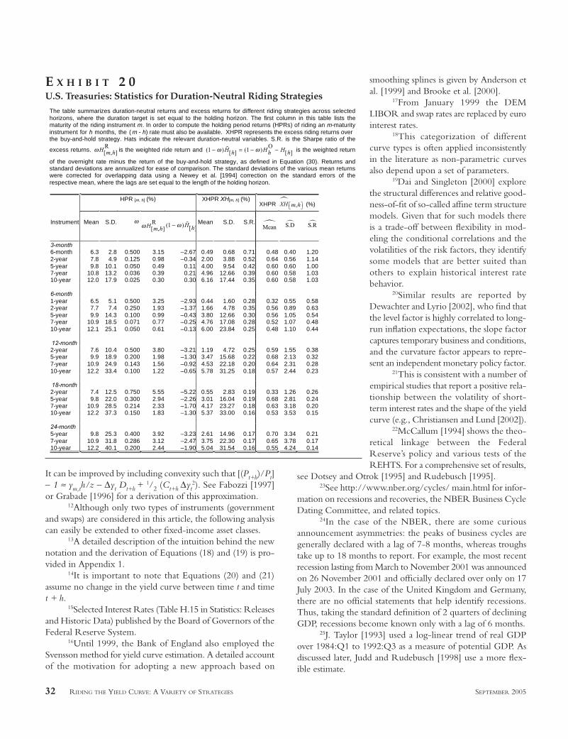
DraftIt can be improved by including convexity such that [(Pt+h)/Pt]– 1 ≈ ym,th/z – ∆yt Dt+h +

1/2 (Ct+h ∆yt2). See Fabozzi [1997]

or Grabade [1996] for a derivation of this approximation.12Although only two types of instruments (government

and swaps) are considered in this article, the following analysiscan easily be extended to other fixed-income asset classes.

13A detailed description of the intuition behind the newnotation and the derivation of Equations (18) and (19) is pro-vided in Appendix 1.

14It is important to note that Equations (20) and (21)assume no change in the yield curve between time t and timet + h.

15Selected Interest Rates (Table H.15 in Statistics: Releasesand Historic Data) published by the Board of Governors of theFederal Reserve System.

16Until 1999, the Bank of England also employed theSvensson method for yield curve estimation. A detailed accountof the motivation for adopting a new approach based on

smoothing splines is given by Anderson etal. [1999] and Brooke et al. [2000].

17From January 1999 the DEMLIBOR and swap rates are replaced by eurointerest rates.

18This categorization of differentcurve types is often applied inconsistentlyin the literature as non-parametric curvesalso depend upon a set of parameters.

19Dai and Singleton [2000] explorethe structural differences and relative good-ness-of-fit of so-called affine term structuremodels. Given that for such models thereis a trade-off between flexibility in mod-eling the conditional correlations and thevolatilities of the risk factors, they identifysome models that are better suited thanothers to explain historical interest ratebehavior.

20Similar results are reported byDewachter and Lyrio [2002], who find thatthe level factor is highly correlated to long-run inflation expectations, the slope factorcaptures temporary business and conditions,and the curvature factor appears to repre-sent an independent monetary policy factor.

21This is consistent with a number ofempirical studies that report a positive rela-tionship between the volatility of short-term interest rates and the shape of the yieldcurve (e.g., Christiansen and Lund [2002]).

22McCallum [1994] shows the theo-retical linkage between the FederalReserve’s policy and various tests of theREHTS. For a comprehensive set of results,

see Dotsey and Otrok [1995] and Rudebusch [1995].23See http://www.nber.org/cycles/ main.html for infor-

mation on recessions and recoveries, the NBER Business CycleDating Committee, and related topics.

24In the case of the NBER, there are some curiousannouncement asymmetries: the peaks of business cycles aregenerally declared with a lag of 7-8 months, whereas troughstake up to 18 months to report. For example, the most recentrecession lasting from March to November 2001 was announcedon 26 November 2001 and officially declared over only on 17July 2003. In the case of the United Kingdom and Germany,there are no official statements that help identify recessions.Thus, taking the standard definition of 2 quarters of decliningGDP, recessions become known only with a lag of 6 months.

25J. Taylor [1993] used a log-linear trend of real GDPover 1984:Q1 to 1992:Q3 as a measure of potential GDP. Asdiscussed later, Judd and Rudebusch [1998] use a more flex-ible estimate.


The table summarizes duration-neutral returns and excess returns for different riding strategies across selectedhorizons, where the duration target is set equal to the holding horizon. The first column in this table lists thematurity of the riding instrument m. In order to compute the holding period returns (HPRs) of riding an m-maturityinstrument for h months, the ( m - h) rate must also be available. XHPR represents the excess riding returns overthe buy-and-hold strategy. Hats indicate the relevant duration-neutral variables. S.R. is the Sharpe ratio of the

excess returns. H[m,h]R

is the weighted ride return and (1 )H[h] = (1 )HhO

H[h] is the weighted return

of the overnight rate minus the return of the buy-and-hold strategy, as defined in Equation (30). Returns andstandard deviations are annualized for ease of comparison. The standard deviations of the various mean returnswere corrected for overlapping data using a Newey et al. [1994] correction on the standard errors of therespective mean, where the lags are set equal to the length of the holding horizon.

HPR [m, h] (%) XHPR XH[m, h] (%)XHPR XH m,h (%)

Instrument Mean S.D.H[m,h]R (1 )H[h]

Mean S.D. S.R.Mean S.D S.R

3-month6-month 6.3 2.8 0.500 3.15 –2.67 0.49 0.68 0.71 0.48 0.40 1.202-year 7.8 4.9 0.125 0.98 –0.34 2.00 3.88 0.52 0.64 0.56 1.145-year 9.8 10.1 0.050 0.49 0.11 4.00 9.54 0.42 0.60 0.60 1.007-year 10.8 13.2 0.036 0.39 0.21 4.96 12.66 0.39 0.60 0.58 1.0310-year 12.0 17.9 0.025 0.30 0.30 6.16 17.44 0.35 0.60 0.58 1.03

6-month1-year 6.5 5.1 0.500 3.25 –2.93 0.44 1.60 0.28 0.32 0.55 0.582-year 7.7 7.4 0.250 1.93 –1.37 1.66 4.78 0.35 0.56 0.89 0.635-year 9.9 14.3 0.100 0.99 –0.43 3.80 12.66 0.30 0.56 1.05 0.547-year 10.9 18.5 0.071 0.77 –0.25 4.76 17.08 0.28 0.52 1.07 0.4810-year 12.1 25.1 0.050 0.61 –0.13 6.00 23.84 0.25 0.48 1.10 0.44

12-month2-year 7.6 10.4 0.500 3.80 –3.21 1.19 4.72 0.25 0.59 1.55 0.385-year 9.9 18.9 0.200 1.98 –1.30 3.47 15.68 0.22 0.68 2.13 0.327-year 10.9 24.9 0.143 1.56 –0.92 4.53 22.18 0.20 0.64 2.31 0.2810-year 12.2 33.4 0.100 1.22 –0.65 5.78 31.25 0.18 0.57 2.44 0.23

18-month2-year 7.4 12.5 0.750 5.55 –5.22 0.55 2.83 0.19 0.33 1.26 0.265-year 9.8 22.0 0.300 2.94 –2.26 3.01 16.04 0.19 0.68 2.81 0.247-year 10.9 28.5 0.214 2.33 –1.70 4.17 23.27 0.18 0.63 3.18 0.2010-year 12.2 37.3 0.150 1.83 –1.30 5.37 33.00 0.16 0.53 3.53 0.15

24-month5-year 9.8 25.3 0.400 3.92 –3.23 2.61 14.96 0.17 0.70 3.34 0.217-year 10.9 31.8 0.286 3.12 –2.47 3.75 22.30 0.17 0.65 3.78 0.1710-year 12.2 40.1 0.200 2.44 –1.90 5.04 31.54 0.16 0.55 4.24 0.14

E X H I B I T 2 0U.S. Treasuries: Statistics for Duration-Neutral Riding Strategies

Draft

26Look-ahead bias arises because of the use of informa-tion in a simulation that would not be available during the timeperiod being simulated. Using lags of variables as they wouldhave been available at the time of the simulation, it

TR is estimatedas πt–3 + r * + 0.5(πt–3 – πt*) + 0.5yt–3.

27In an alternative specification, ∆Taylort is defined as thedifference between the Taylor rule estimate and the actual targetrate, which implies that the Taylor rule not only is useful to pre-dict changes in the federal funds target but also sets the optimallevel. In this instance, there is only mild significance on the pre-dictive power of the Taylor rule. In particular, the Taylor ruledoes well prior to 2000, but then seems to be breaking down.Running the regression from 1989:01 (when the Federal Reservestarted moving in multiples of 25 basis points) to 2000:01 (justbefore the target rate peaked), the predictive power of the dynam-ically estimated Taylor rule is highest. See Exhibit 6.

28Since a minimum of 5 years of out-of-sample data arerequired for a first reasonable Taylor rule estimate, the overallsample size for U.S. government data is reduced by approxi-mately 60 observations.

29One possible explanation for the observation that φ <1 may be stem from the fact that the parameter estimates sufferfrom a downward bias owing to the implied “target rate stick-iness,” i.e., the assumption that the Fed only moves rates inmultiples of 25 basis points.

30The implied futures rate is given by , wherep f

t is the price of the contract at time t. Because the expectedaverage funds rate for the entire contract month is a time-weighted average of the observed rates so far and the expectedrates for the remaining days, as the month end approaches, the futures price gets increasingly determined by past dailymovements in the effective funds rate rather than expectations.Thus, when the FOMC meeting falls on any time after themiddle of the month, we define the next month’s contract asthe “relevant contract.”

31As with the signal from the Taylor rule, we put on ariding trade whenever the market expectations signal does notindicate a rate hike.

32The German Treasury has only recently started auc-tioning six-month discount paper, the Bubills, at regularmonthly intervals.

33Although a swap is a zero-NPV instrument (i.e., notan investment in the strictest sense), a synthetic asset can becreated by receiving the fixed rate of the swap and investingthe proceeds in a deposit that is continuously rolled over tomeet the floating payments. As such, swaps represent AA creditrisk and have less correlation with lower credits except duringa “flight to quality” or other Treasury-driven events.

34According to the BIS Triennial Survey [2005], at theend of June 2004 approximately 37% of the total notional prin-cipal outstanding of $59 trillion was denominated in euros, 34%in dollars, and 12% in yen.

i ptf

tf= −100

35Over the respective sample periods for the different cur-rencies, there are 28 months of recession in the United States,25 months in the United Kingdom, and 61 months in Ger-many.

36For both Treasuries and USD Swaps, using laggedNBER recessions increases excess returns even more—acrossall holding horizons. E.g., for 3-month rides, mean excessreturns increase from 9.92 to 13.12% for Treasuries and from6.84 to 13.72% for Swaps. For Gilts, lagged recessions do slightlyworse and for Swaps the results are broadly unchanged (somehorizons improve; others get marginally worse). For GermanBunds, lagged recessions increase riding returns marginallyacross all holding horizons compared with the “simultaneous”recessions. For EUR Swaps thinqs get worse across the board,though there are still positive excess returns. For some horizons,however, the excess returns become lower than the uncondi-tional ones.

37The returns of the overnight deposits are computed bygeometrically linking daily returns of overnight LIBID ratesfor each month of the sample period. Although we ignore trans-action costs, the duration-neutral riding strategies may incurhigher transaction costs owing the daily rebalancing of theovernight deposit.

38Defined as clean price plus accrued interest up to time t.39Spline functions, such as basis or B-splines, are used in

the context of yield curve estimation. There is sometimes someconfusion among practitioners between spline functions and spline-based interpolation. Whereas the former technique uses polyno-mials in order to approximate (unknown) functions, the latter issimply a specific method to interpolate between two data points.

40For example, at the long end of the yield curve, theSvensson model is constrained to converge to a constant level,directly implying that the unbiased expectation hypothesis holds.

REFERENCES

Anderson, Nicola, and John Sleath. “New Estimates of the UKReal and Nominal Yield Curves.” Bank of England QuarterlyBulletin, No. 4 (1999), pp. 384–392.

Ang, Andrew, and Monika Piazzesi. “A No-Arbitrage VectorAutoregression of Term Structure Dynamics with Macroeco-nomic and Latent Variables.” Journal of Monetary Economics, Vol.50, No. 4 (2003), pp. 745–787.

Ang, Sharon, Lakshman Alles, and Dave Allen. “Riding theYield Curve: An Analysis of International Evidence.” The Journalof Fixed Income, Vol. 8, No. 4 (1998), pp. 57–74.

Bank for International Settlements. “Zero-Coupon YieldCurves: Technical Documentation.” Basel, March 1999.


Draft

Bank for International Settlements. “Triennial Central BankSurvey of Foreign Exchange and Derivatives Market Activity2004.” Basel, March 2005.

Brandt, Michael W., and Kenneth A. Kravajecz. “Price Dis-covery in the U.S. Treasury Market: The Impact of Orderflowand Liquidity on the Yield Curve.” NBER Working PaperSeries 9529, National Bureau of Economic Research, Cam-bridge, MA, February 2003.

Brooke, Martin, Neil Cooper, and Cederic Scholtes. “InferringMarket Interest Rate Expectations from Money Market Rates.”Bank of England Quarterly Bulletin, No. 4 (2000), pp. 392–402.

Campbell, John Y., and Robert J. Shiller. “Yield Spreads andInterest Rate Movements: A Bird’s Eye View.” Review of Eco-nomic Studies, Vol. 58, No. 2 (1991), pp. 495–514.

Chicago Board of Trade. “Reference Guide: CBOT Fed FundsFutures.” Chicago, IL, March 2003.

Christiansen, Charlotte, and Jesper Lund. “Revisiting the Shapeof the Yield Curve: The Effect of Interest Rate Volatility.”Working Paper, Aarhus School of Business, Aarhus, Denmark,February 2002.

Cook, Timothy, and Thomas Hahn. “Interest Rate Expectationsand the Sope of the Money Market Yield Curve.” Federal ReserveBank of Richmond Economic Review, Vol. 76 (1990), pp. 3–26.

Cuthbertson, Keith. Quantitative Financial Economics. Chich-ester: John Wiley & Sons, 1996.

Dai, Qiang, and Kenneth J. Singleton. “Specification Analysisof Affine Term Structure Models.” Journal of Finance, Vol. 55,No. 5 (2000), pp. 1943–1978.

Dewachter, Hans, and Marco Lyrio. “Macro Factors and theTerm Strucutre of Interest Rates.” Research in Management ERS-2003-037, Erasmus Research Institute of Management, Rot-terdam, Netherlands, October 2002.

Dignan, James H. “Nondefault Components of Investment-Grade Bond Spreads.” Financial Analysts Journal, Vol. 59, No.3 (2003), pp. 93–102.

Dotsey, Michael, and Christopher Otrok. “The Rational Expec-tations Hypothesis of the Term Structure, Monetary Policy,and Time-Varying Term Premia.” Federal Reserve Bank of Rich-mond Economic Quarterly, Vol. 81, No. 1 (1995), pp. 65–81.

Duffie, Darrel, and Ming Huang. “Swap Rates and CreditQuality.” Journal of Finance, Vol. 51, No. 3 (1996), pp. 921–949.

Dyl, Edward A., and Michael D. Joehnk. “Riding the YieldCurve: Does it Work?” The Journal of Portfolio Management, Vol.7, No. 3 (1981), pp. 13–17.

Evans, Charles L, and David Marshall. “Economic Determi-nants of the Nominal Treasury Yield Curve.” Working Paper01–16, Federal Reserve Bank of Chicago, Chicago, IL, Sep-tember 2002.

Fabozzi, Frank J., ed., Handbook of Fixed Income Securities, 5thed. Chicago, IL: Irwin Professional Publishing, 1997.

Fehle, Frank. “The Components of Interest Rate Swap Spreads:Theory and International Evidence.” Journal of Futures Markets,Vol. 23, No. 4 (2003), pp. 347–387.

Fisher, Mark E., Douglas Nychka, and David Zervos. “Fit-ting the Term Structure of Interest Rates with SmoothingSplines.” Finance and Economics Discussion Series 95–1,Board of Governors of the Federal Reserve System, Wash-ington, DC, 1995.

Fleming, Michael J., and Eli M. Remolona. “The Term Struc-ture of Announcement Effects.” BIS Working Paper 71, Bankfor International Settlements, Basel, June 1999a.

——.”What Moves Bond Prices?” The Journal of Portfolio Man-agement, Vol. 25, No. 4 (1999b), pp. 28–38.

Garbade, Kenneth D. “Fixed Income Analytics.” Cambridge, MA:MIT Press, 1996.

Gerlach, Stefan, and Frank Smets. “The Term Structure ofEuro-Rates: Some Evidence in Support of the ExpectationsHypothesis.” Journal of International Money and Finance, Vol. 16(1997), pp. 305–321.

Grieves, Robin, and Alan J. Marcus. “Riding the Yield Curve:Reprise.” The Journal of Portfolio Management, Vol. 18, No. 4(1992), pp. 67–76.

Grieves, Robin, Steven V. Mann, Alan J. Marcus, and Pradip-kumar Ramanlal. “Riding the Bill Curve.” The Journal of Port-folio Management, Vol. 25, No. 3 (1999), pp. 74–82.

He, Hua. “Modelling Term Structure of Swap Spreads.”Working paper, Yale School of Management, New Haven, CT,May 2000.

Ilmanen, Antti. “Does Duration Extension Enhance Long-TermExpected Returns.” The Journal of Fixed Income, Vol. 6, No. 2(1996), pp. 23–36.


Draft

——. “Market Rate Expectation and Forward Rates.” TheJournal of Fixed Income, Vol. 6. No. 2 (1996), pp. 8–22.

Ilmanen, Antti, and Rafey Sayood. “Quantitative ForecastingModels and Active Diversification for International Bonds.”The Journal of Fixed Income, Vol. 12, No. 3 (2002), pp. 40–51.

Judd, John P., and Glenn D. Rudebusch. “Taylor’s Rule and theFed: 1970–1997.” Federal Reserve Bank of San Francisco EconomicReview, No. 3 (1998), pp. 3–16.

Knetz, Peter J., Robert Litterman, and Jose A. Scheinkman.“Explorations into Factors Explaining Money Market Returns.”Journal of Finance, Vol. 49, No. 5 (1994), pp. 1861–1882.

Litterman, Robert, and José A. Scheinkman. “Common Fac-tors Affecting Bond Returns.” The Journal of Fixed Income, Vol.1, No. 3 (1991), pp. 49–53.

Mankiw, N. Gregory, and James A. Miron. “The ChangingBehaviour of the Term Structure of Interest Rates.” QuarterlyJournal of Economics, Vol. 101, No. 2 (1986), pp. 211–228.

McCallum, Bennett T. “Monetary Policy and the Term Struc-ture of Interest Rates.” NBER Working Paper Series 4938,National Bureau of Economic Research, Cambridge, MA,December 1994.

Mishkin, Frederic S. “Yield Curve.” NBER Working PaperSeries 3550, National Bureau of Economic Research, Cam-bridge, MA, December 1990.

Nelson, Charles R., and Andrew F. Siegel. “Parsimonious Mod-eling of Yield Curves.” Journal of Business, Vol. 60, No. 4 (1987),pp. 473–489.

Newey, Whitney K., and Kenneth D. West. “Automatic LagSelection in Covariance Matrix Estimation.” Review of EconomicStudies, Vol. 61, No. 4 (1994), pp. 631–653.

Rudebusch, Glenn D. “Federal Reserve Interest Rate Tar-geting, Rational Expectations, and the Term Structure.” Journalof Monetary Economics, 35 (1995), pp. 245–274.

Rudebusch, Glenn D., and Tao Wu. “A Macro-Finance Modelof the Term Structure, Monetary Policy, and the Economy.”Working paper, Federal Reserve Bank of San Francisco, SanFrancisco, CA, September 2003.

Söderström, Ulf. “Predicting Monetary Policy with FederalFunds Futures Prices.” Journal of Futures Markets, Vol. 21, No.4 (2001), pp. 377–391.

Svensson, Lars E.O. “Estimating and Interpreting ForwardInterest Rates: Sweden 1992–1994.” NBER Working PaperSeries 4871, National Bureau of Economic Research, Cam-bridge, MA, September 1994.

Taylor, John B. “Discretion versus Policy Rules in Practice.”Carnegie-Rochester Conference Series on Public Policy, 39 (1993),pp. 195–214.

Taylor, Mark P. “Modelling the Yield Curve.” Economic Journal,102 (1992), pp. 524–537.

Wu, Tao. “Monetary Policy and the Slope Factor in EmpiricalTerm Structure Estimations.” Working paper, Federal ReserveBank of San Francisco, San Francisco, CA, August 2001.

——. “What Makes the Yield Curve Move.” Economic Letter,Federal Reserve Bank of San Francisco, San Francisco, CA,June 2003.

To order reprints of this article, please contact Ajani Malik [email protected] or 212-224-3205.


Documents

Riding the Yield Curve: A Variety of Strategies