Embed Size (px)
Citation preview
A New O(n2) Algorithm for the Symmetric Tridiagonal
Eigenvalue/Eigenvector Problem
by
Inderjit Singh Dhillon
B.Tech. (Indian Institute of Technology, Bombay) 1989
A dissertation submitted in partial satisfaction of the
requirements for the degree of
Doctor of Philosophy
in
Computer Science
in the
GRADUATE DIVISION
of the
UNIVERSITY of CALIFORNIA, BERKELEY
Committee in charge:
Professor James W. Demmel, Chair
Professor Beresford N. Parlett
Professor Phil Colella
1997

The dissertation of Inderjit Singh Dhillon is approved:
Chair Date
Date
Date
University of California, Berkeley
1997
A New O(n2) Algorithm for the Symmetric Tridiagonal
Eigenvalue/Eigenvector Problem
Copyright 1997
by
Inderjit Singh Dhillon
1
Abstract
A New O(n2) Algorithm for the Symmetric Tridiagonal Eigenvalue/Eigenvector
Problem
by
Inderjit Singh Dhillon
Doctor of Philosophy in Computer Science
University of California, Berkeley
Professor James W. Demmel, Chair
Computing the eigenvalues and orthogonal eigenvectors of an n� n symmetric tridiagonal
matrix is an important task that arises while solving any symmetric eigenproblem. All
practical software requires O(n3) time to compute all the eigenvectors and ensure their
orthogonality when eigenvalues are close. In the �rst part of this thesis we review earlier
work and show how some existing implementations of inverse iteration can fail in surprising
ways.
The main contribution of this thesis is a new O(n2), easily parallelizable algorithm
for solving the tridiagonal eigenproblem. Three main advances lead to our new algorithm.
A tridiagonal matrix is traditionally represented by its diagonal and o�-diagonal elements.
Our most important advance is in recognizing that its bidiagonal factors are \better" for
computational purposes. The use of bidiagonals enables us to invoke a relative criterion to
judge when eigenvalues are \close". The second advance comes by using multiple bidiag-
onal factorizations in order to compute di�erent eigenvectors independently of each other.
Thirdly, we use carefully chosen dqds-like transformations as inner loops to compute eigen-
pairs that are highly accurate and \faithful" to the various bidiagonal representations.
Orthogonality of the eigenvectors is a consequence of this accuracy. Only O(n) work per
eigenpair is needed by our new algorithm.
Conventional wisdom is that there is usually a trade-o� between speed and accu-
racy in numerical procedures, i.e., higher accuracy can be achieved only at the expense of
greater computing time. An interesting aspect of our work is that increased accuracy in
2
the eigenvalues and eigenvectors obviates the need for explicit orthogonalization and leads
to greater speed.
We present timing and accuracy results comparing a computer implementation
of our new algorithm with four existing EISPACK and LAPACK software routines. Our
test-bed contains a variety of tridiagonal matrices, some coming from quantum chemistry
applications. The numerical results demonstrate the superiority of our new algorithm. For
example, on a matrix of order 966 that occurs in the modeling of a biphenyl molecule
our method is about 10 times faster than LAPACK's inverse iteration on a serial IBM
RS/6000 processor and nearly 100 times faster on a 128 processor IBM SP2 parallel machine.
Professor James W. DemmelDissertation Committee Chair

iii
To my parents,
for their constant love and support.
iv
Contents
List of Figures vi
List of Tables viii
1 Setting the Scene 1
1.1 Our Goals : : : : : : : : : : : : : : : : : : : : : : : : : : : : : : : : : : : : : 2
1.2 Outline of Thesis : : : : : : : : : : : : : : : : : : : : : : : : : : : : : : : : : 3
1.3 Notation : : : : : : : : : : : : : : : : : : : : : : : : : : : : : : : : : : : : : : 5
2 Existing Algorithms & their Drawbacks 7
2.1 Background : : : : : : : : : : : : : : : : : : : : : : : : : : : : : : : : : : : : 7
2.2 The QR Algorithm : : : : : : : : : : : : : : : : : : : : : : : : : : : : : : : : 9
2.3 Bisection and Inverse Iteration : : : : : : : : : : : : : : : : : : : : : : : : : 11
2.4 Divide and Conquer Methods : : : : : : : : : : : : : : : : : : : : : : : : : : 12
2.5 Other Methods : : : : : : : : : : : : : : : : : : : : : : : : : : : : : : : : : : 13
2.6 Comparison of Existing Methods : : : : : : : : : : : : : : : : : : : : : : : : 14
2.7 Issues in Inverse Iteration : : : : : : : : : : : : : : : : : : : : : : : : : : : : 16
2.8 Existing Implementations : : : : : : : : : : : : : : : : : : : : : : : : : : : : 20
2.8.1 EISPACK and LAPACK Inverse Iteration : : : : : : : : : : : : : : : 22
2.9 Our Approach : : : : : : : : : : : : : : : : : : : : : : : : : : : : : : : : : : : 32
3 Computing the eigenvector of an isolated eigenvalue 34
3.1 Twisted Factorizations : : : : : : : : : : : : : : : : : : : : : : : : : : : : : : 38
3.2 The Eigenvector Connection : : : : : : : : : : : : : : : : : : : : : : : : : : : 44
3.3 Zero Pivots : : : : : : : : : : : : : : : : : : : : : : : : : : : : : : : : : : : : 49
3.4 Avoiding Divisions : : : : : : : : : : : : : : : : : : : : : : : : : : : : : : : : 55
3.4.1 Heuristics for choosing r : : : : : : : : : : : : : : : : : : : : : : : : : 56
3.5 Twisted Q Factorizations | A Digression� : : : : : : : : : : : : : : : : : : 57
3.5.1 \Perfect" Shifts are perfect : : : : : : : : : : : : : : : : : : : : : : : 61
3.6 Rank Revealing Factorizations� : : : : : : : : : : : : : : : : : : : : : : : : : 64
4 Computing orthogonal eigenvectors when relative gaps are large 68
4.1 Bene�ts of High Accuracy : : : : : : : : : : : : : : : : : : : : : : : : : : : : 69
4.2 Tridiagonals Are Inadequate : : : : : : : : : : : : : : : : : : : : : : : : : : : 70
v
4.3 Relative Perturbation Theory for Bidiagonals : : : : : : : : : : : : : : : : : 72
4.4 Using Products of Bidiagonals : : : : : : : : : : : : : : : : : : : : : : : : : : 76
4.4.1 qd-like Recurrences : : : : : : : : : : : : : : : : : : : : : : : : : : : : 78
4.4.2 Roundo� Error Analysis : : : : : : : : : : : : : : : : : : : : : : : : : 83
4.4.3 Algorithm X | orthogonality for large relative gaps : : : : : : : : : 93
4.5 Proof of Orthogonality : : : : : : : : : : : : : : : : : : : : : : : : : : : : : : 94
4.5.1 A Requirement on r : : : : : : : : : : : : : : : : : : : : : : : : : : : 95
4.5.2 Outline of Argument : : : : : : : : : : : : : : : : : : : : : : : : : : : 97
4.5.3 Formal Proof : : : : : : : : : : : : : : : : : : : : : : : : : : : : : : : 99
4.5.4 Discussion of Error Bounds : : : : : : : : : : : : : : : : : : : : : : : 105
4.5.5 Orthogonality in Extended Precision Arithmetic : : : : : : : : : : : 107
4.6 Numerical Results : : : : : : : : : : : : : : : : : : : : : : : : : : : : : : : : 108
5 Multiple Representations 111
5.1 Multiple Representations : : : : : : : : : : : : : : : : : : : : : : : : : : : : : 112
5.2 Relatively Robust Representations (RRRs) : : : : : : : : : : : : : : : : : : 115
5.2.1 Relative Condition Numbers : : : : : : : : : : : : : : : : : : : : : : 116
5.2.2 Examples : : : : : : : : : : : : : : : : : : : : : : : : : : : : : : : : : 119
5.2.3 Factorizations of Nearly Singular Tridiagonals : : : : : : : : : : : : : 123
5.2.4 Other RRRs : : : : : : : : : : : : : : : : : : : : : : : : : : : : : : : 126
5.3 Orthogonality using Multiple Representations : : : : : : : : : : : : : : : : : 126
5.3.1 Representation Trees : : : : : : : : : : : : : : : : : : : : : : : : : : : 127
5.4 Algorithm Y | orthogonality even when relative gaps are small : : : : : : : 132
6 A Computer Implementation 134
6.1 Forming an RRR : : : : : : : : : : : : : : : : : : : : : : : : : : : : : : : : : 135
6.2 Computing the Locally Small Eigenvalues : : : : : : : : : : : : : : : : : : : 136
6.3 An Enhancement using Submatrices : : : : : : : : : : : : : : : : : : : : : : 138
6.4 Numerical Results : : : : : : : : : : : : : : : : : : : : : : : : : : : : : : : : 139
6.4.1 Test Matrices : : : : : : : : : : : : : : : : : : : : : : : : : : : : : : : 140
6.4.2 Timing and Accuracy Results : : : : : : : : : : : : : : : : : : : : : : 143
6.5 Future Enhancements to Algorithm Y : : : : : : : : : : : : : : : : : : : : : 152
7 Conclusions 155
7.1 Future Work : : : : : : : : : : : : : : : : : : : : : : : : : : : : : : : : : : : 156
Bibliography 158
A The need for accurate eigenvalues 169
B Bidiagonals are Better 173
C Multiple representations lead to orthogonality 177
vi
List of Figures
2.1 A typical implementation of Inverse Iteration to compute the jth eigenvector 20
2.2 Eigenvalue distribution in Example : : : : : : : : : : : : : : : : : : : : : : : 21
2.3 Tinvit | EISPACK's implementation of Inverse Iteration : : : : : : : : : 23
2.4 STEIN | LAPACK's implementation of Inverse Iteration : : : : : : : : : : 24
3.1 Twisted Triangular Factorization at k = 3 (the next elements to be annihi-
lated are circled) : : : : : : : : : : : : : : : : : : : : : : : : : : : : : : : : : 40
3.2 Twisted Q Factorization at k = 3 (the next elements to be annihilated are
circled): forming Nk. : : : : : : : : : : : : : : : : : : : : : : : : : : : : : : : 58
3.3 Twisted Triangular Factorization of a Hessenberg matrix at k = 3 (the next
elements to be annihilated are circled) : : : : : : : : : : : : : : : : : : : : : 65
3.4 Twisted Orthogonal Factorization of a Hessenberg matrix at k = 3 (the next
elements to be annihilated are circled) : : : : : : : : : : : : : : : : : : : : : 65
3.5 The above may be thought of as a twisted triangular or orthogonal factor-
ization of a dense matrix at k = 3 (the next elements to be annihilated are
circled) : : : : : : : : : : : : : : : : : : : : : : : : : : : : : : : : : : : : : : 66
4.1 E�ects of roundo� | dstqds transformation : : : : : : : : : : : : : : : : : 85
4.2 E�ects of roundo� | dqds transformation : : : : : : : : : : : : : : : : : : 87
4.3 E�ects of roundo� | dtwqds transformation : : : : : : : : : : : : : : : : : 88
4.4 E�ects of roundo� | LDLT decomposition : : : : : : : : : : : : : : : : : : 90
4.5 dtwqds transformation applied to compute an eigenvector : : : : : : : : : 97
4.6 An eigenvector of a tridiagonal : most of its entries are negligible : : : : : : 106
5.1 Representation Tree | Forming an extra RRR based at 1 : : : : : : : : : : 129
5.2 Representation Tree | Only using the RRR based at 1 : : : : : : : : : : : 130
5.3 Representation Tree | An extra RRR based at 1 is essential : : : : : : : : 131
6.1 Eigenvalue distribution for Biphenyl : : : : : : : : : : : : : : : : : : : : : : 142
6.2 Eigenvalue distribution for SiOSi6 : : : : : : : : : : : : : : : : : : : : : : : 142
6.3 Eigenvalue distribution for Zeolite ZSM-5 : : : : : : : : : : : : : : : : : : : 142
6.4 Absolute and Relative Eigenvalue Gaps for Biphenyl : : : : : : : : : : : : : 152
6.5 Absolute and Relative Eigenvalue Gaps for SiOSi6 : : : : : : : : : : : : : : 152
6.6 Absolute and Relative Eigenvalue Gaps for Zeolite ZSM-5 : : : : : : : : : : 153
vii
C.1 The strong correlation between element growth and relative robustness : : : 181
C.2 Blow up of earlier �gure : X-axis ranges from 1 + 10�8 to 1 + 3:5� 10�8 : : 181
C.3 Relative condition numbers (in the �gure to the right, X-axis ranges from
1 + 10�8 to 1 + 3:5� 10�8) : : : : : : : : : : : : : : : : : : : : : : : : : : : 182
viii
List of Tables
2.1 Summary of xStein's iterations to compute the second eigenvector of T . : : 31
4.1 Timing results on matrices of type 1 : : : : : : : : : : : : : : : : : : : : : : 109
4.2 Accuracy results on matrices of type 1 : : : : : : : : : : : : : : : : : : : : : 109
4.3 Accuracy results on matrices of type 2 : : : : : : : : : : : : : : : : : : : : : 109
6.1 Timing Results : : : : : : : : : : : : : : : : : : : : : : : : : : : : : : : : : : 144
6.2 Timing Results : : : : : : : : : : : : : : : : : : : : : : : : : : : : : : : : : : 145
6.3 Maximum Residual Norms � maxi kT vi � �ivik=n"kTk : : : : : : : : : : : 146
6.4 Maximum Residual Norms � maxi kT vi � �ivik=n"kTk : : : : : : : : : : : 147
6.5 Maximum Dot Products � maxi6=j jvTi vj j=n" : : : : : : : : : : : : : : : : : 148
6.6 Maximum Dot Products � maxi6=j jvTi vj j=n" : : : : : : : : : : : : : : : : : 149
ix
Acknowledgements
The author would like to express his extreme gratitude to Professor Beresford Parlett for
making worthwhile the whole experience of working on this thesis. The author has bene-
�ted greatly from Professor Parlett's expertise, vision and clarity of thought in conducting
research as well as in its presentation. Moreover, helpful discussions over many a lunch has
greatly shaped this work and sparked o� future ideas.
The author is grateful to Professor Demmel for introducing him to the �eld of
numerical linear algebra. Professor Demmel's constant support, numerous suggestions and
careful reading have played a great role in the development of this thesis. The author also
wishes to thank Professor Kahan for much well-received advice, and Dr. George Fann for
many helpful discussions.
The author is also grateful to many friends who have made life in Berkeley an
enriching experience.
This research was supported in part by the Defense Advanced Research Projects
Agency, Contract No. DAAL03-91-C-0047 through a subcontract with the University of
Tennessee, the Department of Energy, Contract No. DOE-W-31-109-Eng-38 through a
subcontract with Argonne National Laboratory, and by the Department of Energy, Grant
No. DE-FG03-94ER25219, and the National Science Foundation Grant No. ASC-9313958,
and NSF Infrastructure Grant No. CDA-9401156.
Part of this work was done when the author was supported by a fellowship, DOE
Contract DE-AC06-76RLO 1830 through the Environmental Molecular Sciences construc-
tion project at Paci�c Northwest National Laboratory (PNNL). The information presented
here does not necessarily re ect the position or the policy of the Government and no o�cial
endorsement should be inferred.
1
Chapter 1
Setting the Scene
In this thesis, we propose a new algorithm for �nding all or a subset of the eigenval-
ues and eigenvectors of a symmetric tridiagonal matrix. The main advance is in being able
to compute numerically orthogonal \eigenvectors" without taking recourse to the Gram-
Schmidt process or a similar technique that explicitly orthogonalizes vectors. All existing
software for this problem needs to do such orthogonalization and hence takes O(n3) time
in the worst case, where n is the order of the matrix. Our new algorithm is the result of
several innovations which enable us to compute, in O(n2) time, eigenvectors that are highly
accurate and numerically orthogonal as a consequence. We believe that the ideas behind
our new algorithm can be gainfully applied to several other problems in numerical linear
algebra.
As an example of the speedups possible due to our new algorithm, the parallel
solution of a 966� 966 dense symmetric eigenproblem, that comes from the modeling of a
biphenyl molecule by the M�ller-Plesset theory, is now nearly 3 times faster than an earlier
implementation [39]. This speedup is a direct consequence of a 10-fold increase in speed of
the tridiagonal solution, which previously accounted for 80-90% of the total time. Detailed
numerical results are presented in Chapter 6.
Before we sketch an outline of our thesis, we list the features of an \ideal" algo-
rithm.
2
1.1 Our Goals
At the onset of our research in 1993, we listed the desirable properties of the
\ultimate" algorithm for computing the eigendecomposition of the symmetric tridiagonal
matrix T . Our wish-list was for
1. An O(n2) algorithm. Such an algorithm would achieve the minimum output com-
plexity in computing all the eigenvectors.
2. An algorithm that guarantees accuracy. Due to the limitations of �nite preci-
sion, we cannot hope to compute the true eigenvalues and ensure that the computed
eigenvectors are exactly orthogonal. A plausible goal is to �nd approximate eigenpairs
(�i; vi), vT
ivi = 1, i = 1; 2; : : : ; n, such that
� the residual norms are small, i.e.,
k(T � �iI)vik = O("kTk); (1.1.1)
� the computed vectors are numerically orthogonal, i.e.,
jvTi vj j = O("); i 6= j; (1.1.2)
where " is the machine precision. For some discussion on how to relate the above
goals to backward errors in T , see [87, Theorem 2.1] and [71]. However it may not
be possible to achieve (1.1.1) and (1.1.2) in all cases and we will aim for bounds that
grow slowly with n.
3. An embarrassingly parallel algorithm that allows independent computation of
each eigenvalue and eigenvector making it easy to implement on a parallel computer.
4. An adaptable algorithm that permits computation of any k of the eigenvalues and
eigenvectors at a reduced cost of O(nk) operations.
We have almost succeeded in accomplishing all these lofty goals. The algorithm
presented at the end of Chapter 5 is an O(n2), embarrassingly parallel and adaptable method
that passes all our numerical tests. Work to further improve this algorithm is still ongoing
and we believe we are very close to a provably accurate algorithm.
3
1.2 Outline of Thesis
The following summarizes the contents of this thesis.
1. In Chapter 2, we give some background explaining the importance of the symmetric
tridiagonal eigenproblem. We then brie y describe some of the existing methods |
the popular QR algorithm, bisection followed by inverse iteration and the relatively
new divide and conquer approach. In Section 2.6, we compare the existing methods in
terms of speed, accuracy and memory requirements discussing how they do not satisfy
all the desirable goals of Section 1.1. Since our new algorithm is related to inverse
iteration, in Section 2.7 we discuss in detail the tricky issues involved in its computer
implementation. In Section 2.8.1, we show how the existing LAPACK and EISPACK
inverse iteration software can fail. The expert reader may skip this chapter and move
on to Chapter 3 where we start describing our new methods.
2. In Chapter 3, we describe in detail the computation of an eigenvector corresponding
to an isolated eigenvalue that has already been computed. We begin by showing how
some of the obvious ways can fail miserably due to the tridiagonal structure. Twisted
factorizations, introduced in Section 3.1, are found to reveal singularity and provide
an elegant mechanism for computing an eigenvector. The method suggested by these
factorizations may be thought of as deterministically \picking a good starting vector"
for inverse iteration thus avoiding the random choices currently used in LAPACK
and solving a question posed by Wilkinson in [136, p.318]. Section 3.4 shows how to
modify this new method in order to eliminate divisions. We then digress a little and
in Sections 3.5 and 3.6 brie y discuss how twisted factorizations can be employed to
reveal the rank of denser matrices and guarantee de ation in perfect shift strategies.
3. In Chapter 4, we show how to independently compute eigenvectors that turn out to
be numerically orthogonal when eigenvalues di�er in most of their digits. Note that
eigenvalues may have tiny absolute gaps without agreeing in any digit, e.g., 10�50 and
10�51 are far apart from each other in a relative sense. We say that such eigenvalues
have large relative gaps. The material of this chapter represents a major advance
towards our goal of an O(n2) algorithm. Sections 4.1 and 4.2 extol the bene�ts of high
accuracy in the computed eigenvalues, and show that for computational purposes, a
bidiagonal factorization of T is \better" than the traditional way of representing T by
4
its diagonal and o�-diagonal elements. In Section 4.3, we review the known properties
of bidiagonal matrices that make them attractive for computation. Section 4.4.1 gives
the qd-like recurrences that allow us to exploit the good properties of bidiagonals,
and in Section 4.4.2 we give a detailed roundo� error analysis of their computer
implementations. Section 4.5 gives a rigorous analysis that proves the numerical
orthogonality of the computed eigenvectors when relative gaps are large. To conclude,
we present a few numerical results in Section 4.6 to verify the above claims.
4. Chapter 5 deals with the case when relative gaps between the eigenvalues are small.
In this chapter, we propose that for each such cluster of eigenvalues, we form an
additional bidiagonal factorization of T +�I where � is close to the cluster, and then
apply the techniques of Chapter 4 to compute eigenvectors that are automatically
numerically orthogonal. The success of this approach depends on �nding relatively
robust representations that are de�ned in Section 5.2. Section 5.3.1 introduces the
concept of a representation tree which is a tool that facilitates proving orthogonality
of the vectors computed using di�erent representations. We present Algorithm Y in
Section 5.4 that also handles the remaining case of small relative gaps. We cannot
prove the correctness of this algorithm as yet but extensive numerical experience
indicates that it is accurate.
5. In Chapter 6 we give a detailed numerical comparison between Algorithm Y and four
existing EISPACK and LAPACK software routines. Section 6.4.1 describes our ex-
tensive collection of test tridiagonals, some of which come from quantum chemistry
applications. We �nd our computer implementation of Algorithm Y to be uniformly
faster than existing implementations of inverse iteration and the QR algorithm. The
speedups range from factors of 4 to about 3500 depending on the eigenvalue distribu-
tion. In Section 6.5, we speculate on further improvements to Algorithm Y.
6. Finally, in Chapter 7, we discuss how some of our techniques may be applicable to
other problems in numerical linear algebra.
In addition to the above chapters, we have included some case studies at the end
of this thesis, which examine various illuminating examples in detail. Much of the material
in the case studies appears scattered in various chapters, but we have chosen to collate and
expand on it at the end, where it can be read independently of the main text.
5
1.3 Notation
We now say a few words about our notation. The reader would bene�t by occa-
sionally reviewing this section during the course of his/her reading of this thesis. We adopt
Householder's conventions and denote matrices by uppercase roman letters such as A, B,
J , T and scalars by lowercase greek letters �, �, , �, or lowercase italic such as ai, bi
etc. We also try to follow the Kahan/Parlett convention of denoting symmetric matrices
by symmetric letters such as A, T and nonsymmetric matrices by B, J etc. In particular,
T stands for a symmetric tridiagonal matrix while J denotes a nonsymmetric tridiagonal.
However, we will occasionally depart from these principles, for example, the letters L and U
will denote lower and upper triangular matrices respectively while D stands for a diagonal
matrix by strong tradition. Overbars will be frequently used when more than one matrix of
a particular type is being considered, e.g., L and ~L. The submatrix of T in rows i through
j will be denoted by T i:j and its characteristic polynomial by �i:j .
We denote vectors by lowercase roman letters such as u, v and z. The ith com-
ponent of the vector v will be denoted by vi or v(i). The (i; j) element of matrix A will be
denoted by Aij . All vectors are n-dimensional and all matrices are n � n unless otherwise
stated. In cases where there are at most n non-trivial entries in a matrix, we will use only
one index to denote these matrix entries, for example L(i) might denote the L(i+1; i) entry
of a unit lower bidiagonal matrix while D(i) or Di can denote the (i; i) element of a diagonal
matrix. The ith column vector of the matrix V will be denoted by vi. We note that this
might lead to some ambiguity, but we will try and explicitly state our notation before such
usage.
We denote the n eigenvalues of a matrix by �1; �2; � � � ; �n, while the n singular
values are denoted by �1; �2; : : : ; �n. Normally we will assume that these quantities are
ordered, i.e., �1 � � � � � �n while �1 � � � � � �n. Note that the eigenvalues are arranged
in increasing order while the singular values are in decreasing order. We have done this to
abide by existing conventions. The ordering is immaterial to most of our presentation, but
we will make explicit the order of arrangement whenever our exposition requires ordering.
Eigenvectors and singular vectors will be denoted by vi and ui. The diagonal matrix of
eigenvalues and singular values will be denoted by � and � respectively, while V and U will
stand for matrices whose columns are eigenvectors and/or singular vectors.
Since �nite precision computations are the driving force behind our work, we
6
brie y introduce our model of arithmetic. We assume that the oating point result of a
basic arithmetic operation � satis�es
fl(x � y) = (x � y)(1 + �) = (x � y)=(1 + �)
where � and � depend on x, y, �, and the arithmetic unit. The relative errors satisfy
j�j < "; j�j < "
for a given " that depends only on the arithmetic unit and will be called the machine
precision. We shall choose freely the form (� or �) that suits the analysis. We also adopt
the convention of denoting the computed value of x by x. In fact, we have already used
some of this notation in Section 1.1.
The IEEE single and double precision formats allow for 24 and 53 bits of precision
respectively. Thus the corresponding " are 2�23 � 1:2 � 10�7 and 2�52 � 2:2 � 10�16
respectively. Whenever " occurs in our analysis it will either denote machine precision
or should be taken to mean \of the order of magnitude of" the machine precision, i.e,
" = O(machine precision).
Just as we did in the above sentence and in equations (1.1.1) and (1.1.2), we
will continue to abuse the \big oh" notation. Normally the O notation, introduced by
Bachmann in 1894 [68, Section 9.2], implies a limiting process. For example, when we say
that an algorithm takes O(n2) time, we mean that the algorithm performs less than Kn2
operations for some constant K as n!1. However in our informal discussions, sometimes
there will not be any limiting process or we may not always make it precise. In the former
case, O will be a synonym for \of the order of magnitude of". Our usage should be clear
from the context. Of course, we will be precise in the statements of our theorems | in fact,
the O notation does not appear in any theorem or proof in this thesis.
We will also be sloppy in our usage of the terms \eigenvalues" and \eigenvec-
tors". An unreduced symmetric tridiagonal matrix has exactly n distinct eigenvalues and
n normalized eigenvectors that are mutually orthogonal. However, in several places we
will use phrases like \the computed eigenvalues are close to the exact eigenvalues" and
\the computed eigenvectors are not numerically orthogonal". In these phrases, we refer to
approximations to the eigenvalues and eigenvectors and we are deliberately sloppy for the
sake of brevity. In a similar vein, we will use \orthogonal" to occasionally mean numerically
orthogonal, i.e., orthogonal to working precision.
7
Chapter 2
Existing Algorithms & their
Drawbacks
In this chapter, we start by giving a quick background to the problem of computing
an eigendecomposition of a dense symmetric matrix for the bene�t of a newcomer. We
then discuss and compare existing methods of solving the resulting tridiagonal problem in
Sections 2.2 through 2.6. Later, in Sections 2.7 and 2.8, we show how various issues that arise
in implementing inverse iteration are handled in existing LAPACK [1] and EISPACK [128]
software, and present some examples where they fail to deliver correct answers. Finally, we
sketch our alternate approach on handling these issues in Section 2.9.
2.1 Background
Eigenvalue computations arise in a rich variety of contexts. A quantum chemist
may compute eigenvalues to reveal the electronic energy states in a large molecule, a struc-
tural engineer may need to construct a bridge whose natural frequencies of vibration lie
outside the earthquake band while eigenvalues may convey information about the stabil-
ity of a market to an economist. A large number of such physically meaningful problems
may be posed as the abstract mathematical problem of �nding all numbers � and non-zero
vectors q that satisfy the equation
Aq = �q;
where A is a real, symmetric matrix of order n. � is called an eigenvalue of the matrix A
while q is a corresponding eigenvector.
8
All eigenvalues of A must satisfy the characteristic equation, det(A��I) = 0 and
since the left hand side of this equation is a polynomial in � of degree n, A has exactly n
eigenvalues. A symmetric matrix further enjoys the properties that
1. all eigenvalues are real, and
2. a complete set of n mutually orthogonal eigenvectors may be chosen.
Thus a symmetric matrix A admits the eigendecomposition
A = Q�QT ;
where � is a diagonal matrix, � = diag(�1; �2; : : : ; �n), and Q is an orthogonal matrix,
i.e., QTQ = I . In the case of an unreduced symmetric tridiagonal matrix, i.e., where all
o�-diagonal elements of the tridiagonal are non-zero, the eigenvalues are distinct while the
eigenvectors are unique up to a scale factor and are mutually orthogonal.
Armed with this knowledge, several algorithms for computing the eigenvalues of
a real, symmetric matrix have been constructed. Prior to the 1950s, explicitly forming
and solving the characteristic equation seems to have been a popular choice. However,
eigenvalues are extremely sensitive to small changes in the coe�cients of the characteristic
polynomial and the inadequacy of this representation became clear with the advent of
the modern digital computer. Orthogonal matrices became, and still remain, the most
important tools of the trade. A sequence of orthogonal transformations,
A0 = A; Ai+1 = QT
iAiQi;
where QT
iQi = I , is numerically stable and preserves the eigenvalues of Ai. Many algorithms
for computing the eigendecomposition of A attempt to construct such a sequence so that
Ai converges to a diagonal matrix. But, Galois' work in the nineteenth century implies that
for n > 4 there can be no �nite m for which Am is diagonal as long as the Qi are computed
by algebraic expressions and taking kth roots. It seems natural to try and transform A to
a tridiagonal matrix instead. In 1954, Givens proposed the reduction of A to tridiagonal
form by using orthogonal plane rotations [62]. However, most current e�cient algorithms
work by reducing A to a tridiagonal matrix T by a sequence of n� 2 orthogonal re ectors,
now named after Householder who �rst introduced them in 1958, see [81]. Mathematically,
T = (QT
n�3 � � �QT
1QT
0 )A(Q0Q1 � � �Qn�3) = ZTAZ
9
The eigendecomposition of T may now be found as
T = V �V T ; (2.1.1)
where V TV = I , and back-transformation may be used to �nd the eigenvectors of A,
A = (ZV )�(ZV )T = Q�QT :
The tridiagonal eigenproblem is one of the most intensively studied problems in numerical
linear algebra. A variety of methods exploit the tridiagonal structure to compute (2.1.1).
Extensive research has led to plenty of software, especially in the linear algebra software
libraries, EISPACK [128] and the more recent LAPACK [1]. We will examine existing
algorithms and related software in the next section.
We now brie y discuss the relative costs of the various components involved in
solving the dense symmetric eigenproblem. Reducing A to tridiagonal form by Householder
transformations costs about 43n3 multiplications and additions, while back-transformation to
get the eigenvectors of A from the tridiagonal solution needs 2n3 multiplication and addition
operations. The cost of solving the tridiagonal eigenproblem varies according to the method
used and the numerical values in the matrix. If the distribution of eigenvalues is favorable
some methods may solve such a tridiagonal problem in O(n2) time. However, all existing
software takes kn3 operations in the worst case, where k is a modest number that can vary
from 4 to 12. In many cases of practical importance, the tridiagonal problem can indeed be
the bottleneck in the total computation. The extent to which it is a bottleneck can be much
greater than suggested by the above numbers because the other two phases, Householder
reduction and back-transformation can exploit fast matrix-multiply based operations [12,
45], whereas most algorithms for the tridiagonal problem are sequential in nature and/or
cannot be expressed in terms of matrix multiplication. We now discuss these existing
algorithms.
2.2 The QR Algorithm
Till recently, the method of choice for the symmetric tridiagonal eigenproblem was
the QR Algorithm which was independently invented by Francis [59] and Kublanovskaja [95].
The QR method is a remarkable iteration process,
T0 = T;
10
Ti � �iI = QiRi; (2.2.2)
Ti+1 = RiQi + �iI; i = 0; 1; 2; : : :
where QT
iQi = I , Ri is upper triangular and �i is a shift chosen to accelerate convergence.
The o�-diagonal elements of Ti are rapidly driven to zero by this process. Francis, helped
by Strachey and Wilkinson, was the �rst to note the invariance of the tridiagonal form and
incorporate shifts in the QR method. These observations make the method computationally
viable. The initial success of the method sparked o� an incredible amount of research into
the QR method, which carries on till this day. Several shift strategies were proposed and
convergence properties of the method studied. The ultimate cubic convergence of the QR
algorithm with suitable shift strategies was observed by both Kahan andWilkinson. In 1968,
Wilkinson proved that the tridiagonal QL iteration (the QL method is intimately related
to the QR method) always converges using his shift strategy. A simpler proof of global
convergence is due to Ho�man and Parlett, see [79]. An excellent treatment of the QR
method is given by Parlett in [110].
Each orthogonal matrix Qi in (2.2.2) is a product of n � 1 elementary rotations,
known as Givens rotations [62]. The tridiagonal matrices Ti converge to diagonal form
that gives the eigenvalues of T . The eigenvector matrix of T is then given by the product
Q1Q2Q3 � � �. When only eigenvalues are desired, the QR transformation can be reorganized
to eliminate all square roots that are required to form the Givens rotations. This was �rst
observed by Ortega and Kaiser in 1963 [109] and a fast, stable algorithm was developed
by Pal, Walker and Kahan (PWK) in 1968-69 [110]. Since a square root operation can be
about 20 or more times as expensive as addition or multiplication, this yields a much faster
method. In particular, the PWK algorithm �nds all eigenvalues of T in approximately 9n2
multiply and add operations and 3n2 divisions, with the assumption that 2 QR iterations
are needed per eigenvalue. However, when eigenvectors are desired, the product of all the
Qi must be accumulated during the algorithm. The O(n2) square root operations cannot be
eliminated in this process and approximately 6n3 multiplications and additions are needed
to �nd all the eigenvalues and eigenvectors of T . In the hope of cutting down this work
by half, Parlett suggested the alternate strategy of computing the eigenvalues by the PWK
algorithm, and then executing the QR algorithm using the previously computed eigenvalues
as origin shifts to �nd the eigenvectors [110, p.173]. However this perfect shift strategy was
not found to work much better than Wilkinson's shift strategy, taking an average of about
11
2 QR iterations per eigenvalue [69, 98].
2.3 Bisection and Inverse Iteration
In 1954, Wallace Givens proposed the method of bisection to �nd some or all of
the eigenvalues of a real, symmetric matrix [62]. This method is based on the availability of
a simple recurrence to count the number of eigenvalues less than a oating point number �.
Let �j(�) = det(�I�T 1:j) be the characteristic polynomial of the leading principal
j� j submatrix of T . The sequence f�0; �1; : : : ; �ng, where �0 = 1 and �1 = ��T11, forms
a Sturm sequence of polynomials. The tridiagonal nature of T allows computation of �j(�)
using the three-term recurrence
�j+1(�) = (�� Tj+1;j+1)�j(�)� T 2j+1;j�j�1(�): (2.3.3)
The number of sign agreements in consecutive terms of the numerical sequence
f�i(�); i = 0; 1; : : : ; ng equals the number of eigenvalues of T less than �. Based on this
recurrence, Givens devised a method that repeatedly halves the size of an interval that
contains at least one eigenvalue. However, it was soon observed that recurrence (2.3.3) was
prone to over ow with a limited exponent range. An alternate recurrence that computes
dj(�) = �j(�)=�j�1(�) is now used in most software [89],
dj+1(�) = (�� Tj+1;j+1)� T 2j+1;j=dj(�); d1(�) = �� T11:
The bisection algorithm permits an eigenvalue to be computed in about 2bn addi-
tion and bn division operations where b is the number of bits of precision in the numbers
(b = 24 in IEEE single while b = 53 in IEEE double precision arithmetic). Thus all eigenval-
ues may be found in O(bn2) operations. Faster iterations that are superlinearly convergent
can beat bisection and we give some references in Section 2.5.
Once an accurate eigenvalue approximation � is known, the method of inverse
iteration may be used to compute an approximate eigenvector [118, 87] :
v(0) = b; (A� �I)v(i+1) = � (i)v(i); i = 0; 1; 2; : : : ;
where b is the starting vector and � (i) is a scalar.
Earlier fears about loss of accuracy in solving the linear system given above due to
the near singularity of T � �I were allayed in [119]. Inverse iteration delivers a vector v that
12
has a small residual, i.e. small k(T��I)vk, whenever � is close to �. However small residualnorms do not guarantee orthogonality of the computed vectors when eigenvalues are close
together. A commonly used \remedy" for clusters of eigenvalues is to orthogonalize each ap-
proximate eigenvector, as soon as it is computed, against previously computed eigenvectors
in the cluster. Typical implementations orthogonalize using the modi�ed Gram-Schmidt
method.
The amount of work required by inverse iteration to compute all the eigenvectors
of a symmetric tridiagonal matrix strongly depends upon the distribution of eigenvalues.
If eigenvalues are well-separated, then O(n2) operations are su�cient. However, when
eigenvalues are close, current implementations can take up to 10n3 operations due to the
orthogonalization.
2.4 Divide and Conquer Methods
In 1981, Cuppen proposed a solution to the symmetric tridiagonal eigenproblem
that was meant to be e�cient for parallel computation [25, 46]. It is quite remarkable that
this method can also be faster than other implementations on a serial computer!
The matrix T may be expressed as a modi�cation of a direct sum of two smaller
tridiagonal matrices. This modi�cation may be a rank-one update [15], or may be ob-
tained by crossing out a row and column of T [72]. The eigenproblem of T can then be
solved in terms of the eigenproblems of the smaller tridiagonal matrices, and this may be
done recursively. For several years after its inception, it was not known how to guaran-
tee numerically orthogonality of the eigenvector approximations obtained by this approach.
However in 1992, Gu and Eisenstat found a clever solution to this problem, and paved the
way for robust software based on their algorithms [72, 73, 124] and Li's work on a faster
zero-�nder [102].
The main reason for the unexpected success of divide and conquer methods on
serial machines is de ation, which occurs when an eigenpair of a submatrix of T is an ac-
ceptable eigenpair of a larger matrix. For symmetric tridiagonal matrices, this phenomenon
is quite common. The greater the amount of de ation, the lesser is the work required in
these methods. The amount of de ation depends on the distribution of eigenvalues and
on the structure of the eigenvectors. In the worst case when no de ation occurs O(n3)
operations are needed, but on matrices where eigenvalues cluster and the eigenvector ma-
13
trix contains many tiny entries, substantial de ation occurs and many fewer than O(n3)
operations are required [73].
In [71, 73], Gu and Eisenstat show that by using the fast multipole method of
Carrier, Greengard and Rokhlin [70, 16], the complexity of solving the symmetric tridiagonal
eigenproblem can be considerably lowered. All the eigenvalues and eigenvectors can be found
in O(n2) operations while all the eigenvalues can be computed in O(n log2 n) operations.
In fact, the latter method also �nds the eigenvectors but in an implicit factored form
(without assembling the n2 entries of all the eigenvectors) that allows multiplication of the
eigenvector matrix by a vector in about n2 operations. However, the constant factor in
the above operation counts is quite high, and matrices encountered currently are not large
enough for these methods to be viable. There is no software available as yet that uses the
fast multipole method for the eigenproblem.
2.5 Other Methods
The oldest method for solving the symmetric eigenproblem is one due to Jacobi
that dates back to 1846 [86], and was rediscovered by von Neumann and colleagues in
1946 [7]. Jacobi's method does not reduce the dense symmetric matrix A to tridiagonal
form, as most other methods do, but instead works on A. It performs a sequence of plane
rotations each of which annihilates an o�-diagonal element (which is �lled in during later
steps). There are a variety of Jacobi methods that di�er solely in their strategies for
choosing the next element to be annihilated. All good strategies tend to diminish the o�-
diagonal elements, and the resulting sequence of matrices converges to the diagonal matrix
of eigenvalues. Jacobi methods cost O(n3) or more operations but the constant is larger
than in any of the algorithms discussed above. Despite their slowness, these methods are
still valuable as they seem to be more accurate than other methods [37]. They can also be
quite fast on strongly diagonally dominant matrices.
The bisection algorithm discussed in Section 2.3 is a reliable way to compute
eigenvalues. However, it can be quite slow and there have been many attempts to �nd faster
zero-�nders such as the Rayleigh Quotient Iteration [110], Laguerre's method [90, 113] and
the Zeroin scheme [31, 13]. These zero-�nders can considerably speed up the computation
of isolated eigenvalues but they seem to stumble when eigenvalues cluster.
Homotopy methods for the symmetric eigenproblem were suggested by Chu in [23,
14
24]. These methods start from an eigenvalue of a simpler matrix D and follow a smooth
curve to �nd an eigenvalue of A(t) � D + t(A � D). D was chosen to be the diagonal
of the tridiagonal in [103], but greater success was obtained by taking D to be a direct
sum of submatrices of T [105, 99]. An alternate divide and conquer method that �nds the
eigenvalues by using Laguerre's iteration instead of homotopy methods is given in [104].
The corresponding eigenvectors in these methods are obtained by inverse iteration.
2.6 Comparison of Existing Methods
All currently implemented software for �nding all the eigenvalues and eigenvectors
of a symmetric tridiagonal matrix requires O(n3) work in the worst case. The fastest current
implementation is the divide and conquer method of [73]. As mentioned in Section 2.4,
many fewer than O(n3) operations are needed when heavy de ation occurs. In fact, for
some matrices, such as a small perturbation of the identity matrix, just O(n) operations
are su�cient to solve the eigenproblem. This method was designed to work well on parallel
computers, o�ering both task and data parallelism [46]. E�cient parallel implementations
are not straightforward to program, and the decision to switch from task to data parallelism
depends on the characteristics of the underlying machine [17]. Due to such complications, all
the currently available parallel software libraries, such as ScaLAPACK [22] and PeIGS [52],
use algorithms based on bisection and inverse iteration. A drawback of the current divide
and conquer software in LAPACK is that it needs extra workspace of more than 2n2 oating
point numbers, which can be prohibitively excessive for large problems. Also, the divide
and conquer algorithm does not allow the computation of a subset of the eigenvalues and
eigenvectors at a proportionately reduced cost.
The bisection algorithm enables any subset of k eigenvalues to be computed with
O(nk) operations. Each eigenvalue can be found independently and this makes it suitable for
parallel computation. However, bisection is slow if all the eigenvalues are needed. A faster
root-�nder, such as Zeroin [31, 13], speeds up computation when an eigenvalue is isolated
in an interval. Multisection maintains the simplicity of bisection and in certain situations,
can speed up the performance on a parallel machine [106, 11, 127]. When the k eigenvalues
are well separated, inverse iteration can �nd the eigenvectors independently, each in O(n)
time. However, to �nd eigenvectors of k close eigenvalues, all existing implementations
resort to reorthogonalization and this costs O(nk2) operations. Orthogonalization can also
15
lead to heavy communication in a parallel implementation. The computed eigenvectors
may also not be accurate enough in some rare cases. See Section 2.8.1 for more details.
Despite these drawbacks, the embarrassingly parallel nature of bisection followed by inverse
iteration makes it easy and e�cient to program on a parallel computer. As a result, this is
the method that has been implemented in current software libraries for distributed memory
computers, such as ScaLAPACK [47], PeIGS [52, 54] and in [75].
Like the recent divide and conquer methods, the QR algorithm guarantees numer-
ical orthogonality of the computed eigenvectors. The O(n2) computation performed in the
QR method to �nd all the eigenvalues is sequential in nature and is not easily parallelized
on modern parallel machines despite the attempts in [96, 132, 93]. However, the O(n3) com-
putation in accumulating the Givens' rotations into the eigenvector matrix is trivially and
e�ciently parallelized, see [3] for more details. But the higher operation count and inability
to exploit fast matrix-multiply based operations make the QR algorithm much slower than
divide and conquer and also, slower on average than bisection followed by inverse iteration.
Prior to beginning this work, we were hopeful of �nding an algorithm that could
ful�l the rather ambitious goals of Section 1.1 because
� when eigenvalues are well separated, bisection followed by inverse iteration requires
O(n2) operations, and
� when eigenvalues are clustered, the divide and conquer method is very fast.
The above observations suggest a hybrid algorithm that solves clusters by the
divide and conquer algorithm and computes eigenvectors of isolated eigenvalues by inverse
iteration. Indeed such an approach has been taken in [60]. Another alternative is to perform
bisection and inverse iteration in higher precision. This may be achieved by simulating
quadrupled precision, i.e., doubling the precision of the machine's native arithmetic, in
software in an attempt to obviate the need for orthogonalization [38].
We choose to take a di�erent approach in our thesis. By revisiting the problem
at a more fundamental level, we have been able to arrive at an algorithm that shares
the attractive features of inverse iteration and the divide and conquer method. Since our
approach can be viewed as an alternate way of doing inverse iteration, we now look in detail
at the issues involved in any implementation of inverse iteration. Although many surprising
aspects of current implementations are revealed by our careful examination, the reader who
is pressed for time may skip on to Chapter 3 for the main results of this thesis. The material
16
in the upcoming sections also appears in [40].
2.7 Issues in Inverse Iteration
Inverse Iteration is a method to �nd an eigenvector when an approximate eigen-
value � is known :
v(0) = b; (A� �I)v(i+1) = � (i)v(i); i = 0; 1; 2; : : : : (2.7.4)
Here b is the starting vector. Usually kv(i)k = 1 and � (i) is a scalar chosen to try
and make kv(i+1)k � 1. We now list the key issues that arise in a computer implementation.
I. Choice of shift. Given an approximate eigenvalue �, what shift � should be chosen
when doing the inverse iteration step :
(A� �I)v(i+1) = � (i)v(i) ? (2.7.5)
Should � always equal �? How close should � be to an eigenvalue? Should the
accuracy of � be checked?
II. Direction of starting vector. How should b be chosen?
III. Scaling of right hand side. When the shift � is very close to an eigenvalue,
k(A� �I)�1k is large and solving (2.7.5) may result in over ow. Can � (i) be chosen
to prevent over ow?
IV. Convergence Criterion. When does an iterate v(i) satisfy (1.1.1)? If the criterion
for acceptance is too strict, the iteration may never stop and the danger of too loose
a criterion is that poorer approximations than necessary may be accepted.
V. Orthogonality. Will the vectors for di�erent eigenvalues computed by (2.7.4) be
numerically orthogonal? If not, what steps must be taken to ensure orthogonality?
We now examine these issues in more detail. Before we do so, it is instructive to
look at the �rst iterate of (2.7.5) in the eigenvector basis. Suppose that b is a starting vector
with kbk2 = 1, and that � is an approximation to the eigenvalue �1. Writing b in terms of
the eigenvectors, b =P
n
i=1 �ivi, we get, in exact arithmetic
v1 = � (1)(A� �I)�1b = � (1)
�1
�1 � �v1 +
nXi=2
�i
�i � �vi
!
17
) v1 =�1�
(1)
�1 � �
v1 +
nXi=2
�i
�1
�1 � �
�i � �vi
!: (2.7.6)
I. Choice of shift. The above equation shows that for v1 to be a good approximation
to v1, � must be close to �1. But in such a case, the linear system (2.7.5) is ill-
conditioned and small changes in � or A can lead to large changes in the solution
v(i+1). Initially, it was feared that roundo� error would destroy these calculations
in �nite precision arithmetic. However Wilkinson showed that the errors made in
computing v(i+1), although large, are almost entirely in the direction of v1 when �1
is isolated. Since we are interested only in computing the direction of v1 these errors
pose no danger, see [119]. Thus to compute the eigenvector of an isolated eigenvalue,
the more accurate the shift is the better is the approximate eigenvector.
It is common practice now to compute eigenvalues �rst, and then invoke inverse it-
eration with very accurate �. Due to the fundamental limitations of �nite precision
arithmetic, eigenvalues of symmetric matrixes can, in general, only be computed to
a guaranteed accuracy of O("kAk) [110]. Even when a very accurate eigenvalue ap-
proximation is available, the following may in uence the choice of the shift when more
than one eigenvector is desired.
� The pairing problem. In [20], Chandrasekaran gives a surprising example
showing how inverse iteration can fail to give small residuals in exact arithmetic
if the eigenvalues and eigenvectors are not paired up properly. We reproduce
the example in Section 2.8. To prevent such an occurrence, Chandrasekaran
proposes perturbing the eigenvalue approximations so that each shift used for
inverse iteration lies to the left of, i.e., is smaller than, its nearest eigenvalue (see
Example 2.8.1 for more details).
� The separation problem. The solution v(i+1) in (2.7.5) is very sensitive to
small changes in � when there is more than one eigenvalue near �. In [136,
p.329], Wilkinson notes that
`The extreme sensitivity of the computed eigenvector to very small
changes in � [� in our notation] may be turned to practical advantage
and used to obtain independent eigenvectors corresponding to coincident
or pathologically close eigenvalues'.
Wilkinson proposed that such nearby eigenvalues be `arti�cially separated' by a
tiny amount.
18
II. Direction of starting vector. From (2.7.6), assuming that j�1 � �j � j�i � �j fori 6= 1, v1 is a good approximation to v1 provided that �1 is not \negligible", i.e., the
starting vector must have a non-negligible component in the direction of the desired
eigenvector. In [136, pp.315-321], Wilkinson investigates and rejects the choice of e1
or en as a starting vector (where ei is the ith column of the n�n identity matrix). ek
is a desirable choice for a starting vector if the kth component of v1 is above average
(> 1=pn). In the absence of an e�cient procedure to �nd such a k, Wilkinson
proposed choosing PLe as the starting vector, where T � �I = PLU and e is the
vector of all 1's [134, 136]. A random starting vector is a popular choice since the
probability that it has a negligible component in the desired direction is extremely
low, see [87] for a detailed study.
III. Scaling of right hand side. Equation (2.7.6) implies that kv1k = O(j� (1)=(�1��)j)where � (1) is the scale factor in the �rst iteration of (2.7.5). If � is very close to an
eigenvalue, kv1k can be very large and over owmay occur and lead to breakdown in the
eigenvector computation. To avoid such over ow, � (1) should be chosen appropriately
to scale down the right hand side. This approach is taken in EISPACK and LAPACK.
IV. Convergence Criterion. In the iteration (2.7.4), when is v(i+1) an acceptable eigen-
vector? The residual norm is
k(A� �1I)v(i+1)k
kv(i+1)k =k� (i) � v(i)kkv(i+1)k : (2.7.7)
The factor kv(i+1)k=k� (i) � v(i)k is called the norm growth. To guarantee (1.1.1), v(i+1)
is usually accepted when the norm growth is O(1=n"kTk), see [136, p.324] for details.For the basic iteration of (2.7.4) this convergence criterion can always be met in
a few iterations, provided the starting vector is not pathologically de�cient in the
desired eigenvector and j�1 � �1j = O(n"kTk). As we have mentioned before, these
requirements are easily met.
Since the eigenvalue approximations are generally input to inverse iteration, what
should the software do if the input approximations are not accurate, i.e., bad data
is input to inverse iteration? We believe that the software should raise some sort
of error ag either by testing for the accuracy of the input eigenvalues, or through
non-convergence of the iterates.
19
When �1 is isolated, a small residual implies orthogonality of the computed vector to
other eigenvectors (see (2.7.8) below). However when �1 is in a cluster, goal (1.1.2)
is not automatic. As we now discuss, the methods used to compute numerically
orthogonal vectors can impact the choice of the convergence criterion.
V. Orthogonality. Standard perturbation theory [110, Section 11-7] says that if v is a
unit vector, � is the eigenvalue closest to � and v is �'s eigenvector then
j sin 6 (v; v)j � kAv � �vkgap(�)
(2.7.8)
where gap(�) = min�i 6=� j�� �ij.
In particular, the above implies that the simple iteration scheme of (2.7.4) cannot
guarantee orthogonality of the computed \eigenvectors" when eigenvalues are close.
To achieve numerical orthogonality, current implementations modify (2.7.4) by explic-
itly orthogonalizing each iterate against eigenvectors of nearby eigenvalues that have
already been computed.
However, orthogonalization can fail if the vectors to be orthogonalized are close to
being parallel. When this happens, two surprising di�culties arise :
� The orthogonalized vectors may not provide an orthogonal basis of the desired
subspace.
� Orthogonalization may lead to cancellation and a decrease in norm of the iterate.
Thus a simple convergence criterion (as suggested above in issue IV) may not be
reached.
The eigenvalues found by the QR algorithm and the divide and conquer method can
be in error by O("kTk). As a result, approximations to small eigenvalues may not
be correct in most of their digits. Thus computed eigenvalues may not be accurate
\enough" leading to the above failures surprisingly often. We give examples of such
occurrences in Section 2.8.1. In response to the above problems, Chandrasekaran
proposes a new version of inverse iteration that is considerably di�erent from the
EISPACK and LAPACK implementations in [20]. The di�erences include an alternate
convergence criterion. The drawback of this new version is the potential increase in
the amount of computation required.
20
Inverse Iteration(A,�)
/* assume that v1; v2; : : : ; vj�1 have been computed, and �i; �i+1; : : : ; �j form a cluster */
Choose a starting vector bj ;
Orthogonalize bj against vi; vi+1; : : : ; vj�1;
l = 0; v(0) = bj ;
do
l = l+ 1;
Solve (A� �jI)v(l+1) = � (l)v(l);
Orthogonalize v(l+1) against vi; vi+1; : : : ; vj�1;
while(kv(l+1)k=k� (l)v(l)k is not \big" enough)
vj = v(l+1)=kv(l+1)k;
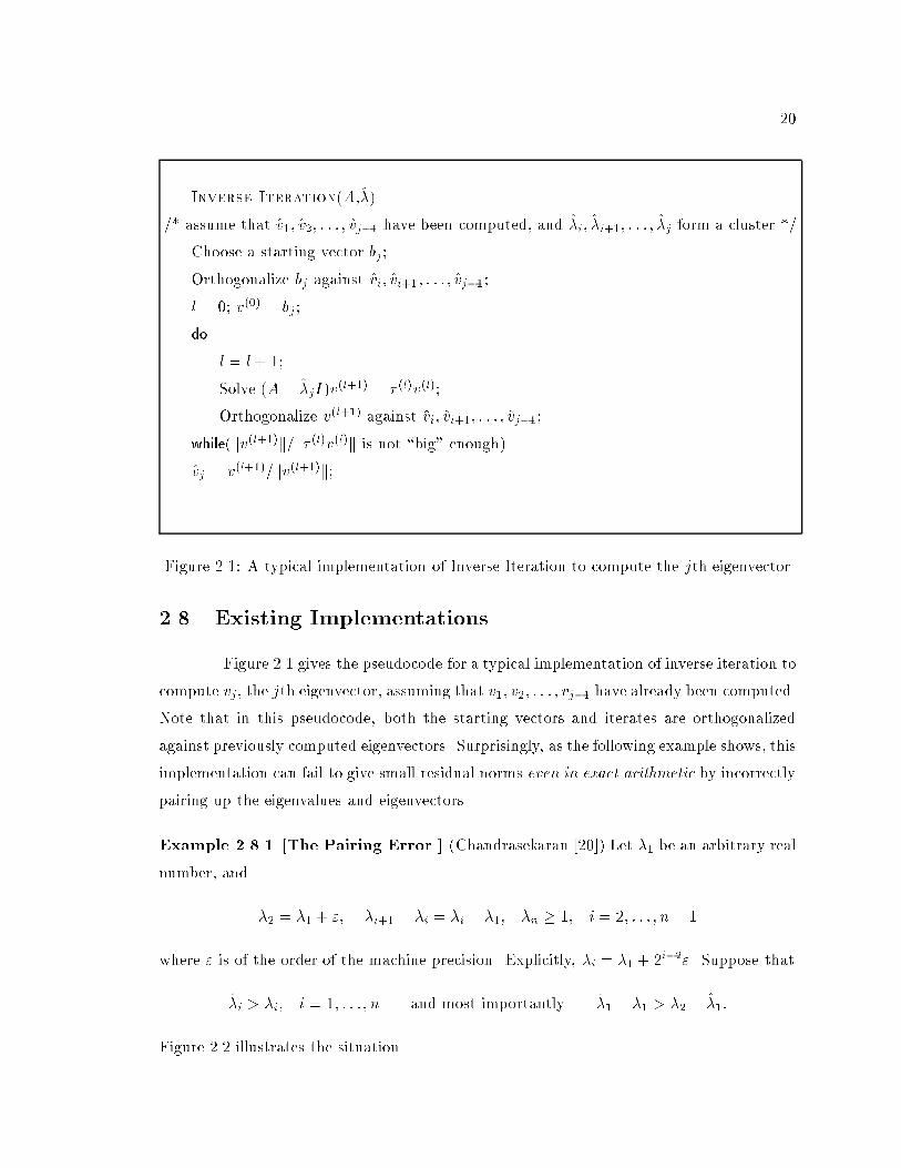
Figure 2.1: A typical implementation of Inverse Iteration to compute the jth eigenvector
2.8 Existing Implementations
Figure 2.1 gives the pseudocode for a typical implementation of inverse iteration to
compute vj , the jth eigenvector, assuming that v1; v2; : : : ; vj�1 have already been computed.
Note that in this pseudocode, both the starting vectors and iterates are orthogonalized
against previously computed eigenvectors. Surprisingly, as the following example shows, this
implementation can fail to give small residual norms even in exact arithmetic by incorrectly
pairing up the eigenvalues and eigenvectors.
Example 2.8.1 [The Pairing Error.] (Chandrasekaran [20]) Let �1 be an arbitrary real
number, and
�2 = �1 + "; �i+1 � �i = �i � �1; �n � 1; i = 2; : : : ; n� 1
where " is of the order of the machine precision. Explicitly, �i = �1 + 2i�2". Suppose that
�i > �i; i = 1; : : : ; n and most importantly �1 � �1 > �2 � �1:
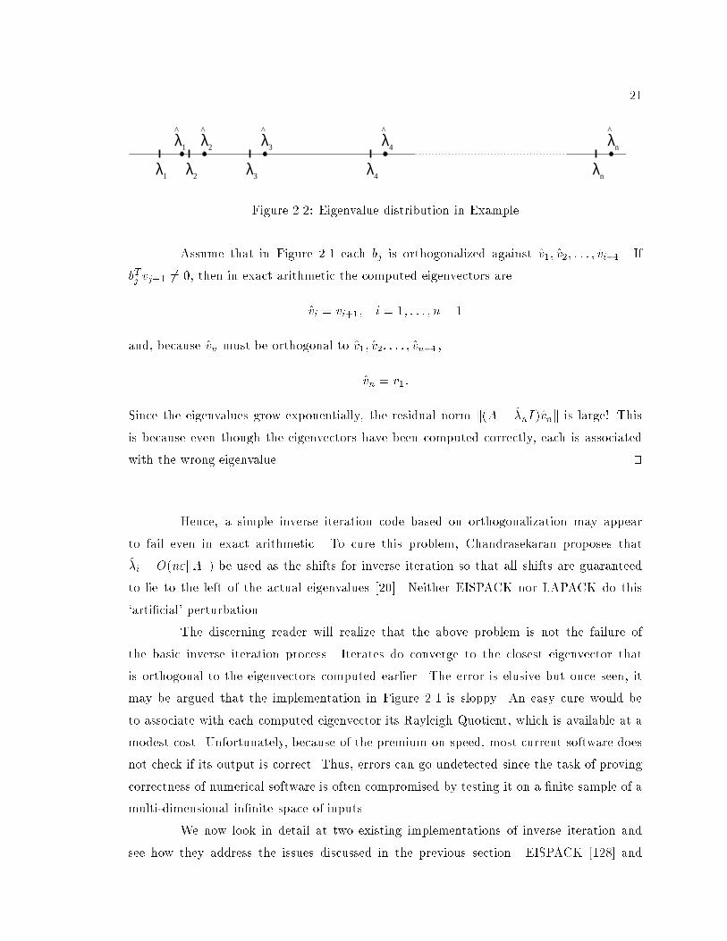
Figure 2.2 illustrates the situation.
21
λ λ λ λ1 2 43
λ λ λ λ λ
λn
1 2 43 n
^^^ ^ ^
Figure 2.2: Eigenvalue distribution in Example
Assume that in Figure 2.1 each bj is orthogonalized against v1; v2; : : : ; vi�1. If
bTjvj+1 6= 0, then in exact arithmetic the computed eigenvectors are
vi = vi+1; i = 1; : : : ; n� 1
and, because vn must be orthogonal to v1; v2; : : : ; vn�1,
vn = v1:
Since the eigenvalues grow exponentially, the residual norm k(A � �nI)vnk is large! This
is because even though the eigenvectors have been computed correctly, each is associated
with the wrong eigenvalue. tu
Hence, a simple inverse iteration code based on orthogonalization may appear
to fail even in exact arithmetic. To cure this problem, Chandrasekaran proposes that
�i � O(n"kAk) be used as the shifts for inverse iteration so that all shifts are guaranteed
to lie to the left of the actual eigenvalues [20]. Neither EISPACK nor LAPACK do this
`arti�cial' perturbation.
The discerning reader will realize that the above problem is not the failure of
the basic inverse iteration process. Iterates do converge to the closest eigenvector that
is orthogonal to the eigenvectors computed earlier. The error is elusive but once seen, it
may be argued that the implementation in Figure 2.1 is sloppy. An easy cure would be
to associate with each computed eigenvector its Rayleigh Quotient, which is available at a
modest cost. Unfortunately, because of the premium on speed, most current software does
not check if its output is correct. Thus, errors can go undetected since the task of proving
correctness of numerical software is often compromised by testing it on a �nite sample of a
multi-dimensional in�nite space of inputs.
We now look in detail at two existing implementations of inverse iteration and
see how they address the issues discussed in the previous section. EISPACK [128] and
22
LAPACK [1] are linear algebra software libraries that contain routines to solve various
eigenvalue problems. EISPACK's implementation of inverse iteration is named Tinvit
while LAPACK's inverse iteration subroutine is called xStein1 (Stein is an acronym for
Symmetric Tridiagonal's Eigenvectors through Inverse Iteration). xStein was developed to
be more accurate than Tinvit as the latter was found to deliver less than satisfactory results
in several test cases. In order to achieve accuracy comparable to that of the divide and
conquer and QR/QL methods, the search for a better implementation of inverse iteration
led to xStein [87]. However, as we will see in Section 2.8.1, xStein also su�ers from some
of the same problems as Tinvit in addition to introducing a new serious error.
Both EISPACK and LAPACK solve the dense symmetric eigenproblem by re-
ducing the dense matrix to tridiagonal form by Householder transformations [81], and then
�nding the eigenvalues and eigenvectors of the tridiagonal matrix. Both Tinvit and xStein
operate on a symmetric tridiagonal matrix. In the following, we will further assume that
the tridiagonal is unreduced, i.e., all the o�-diagonal elements are nonzero.
2.8.1 EISPACK and LAPACK Inverse Iteration
Figure 2.3 gives the pseudocode for Tinvit [128, 118] while Figure 2.4 outlines the
pseudocode for xStein as it appears in LAPACK release 2:0. The latter code has changed
little since it was �rst released in 1992. It is not necessary for the reader to absorb all
details of the implementations given in Figures 2.3 and 2.4 to follow the ensuing discussion.
We provide the pseudocodes as references in case the reader needs to look in detail at a
particular aspect of the implementations.
In each iteration, Tinvit and xStein solve the scaled linear system (T��I)y = �b
by Gaussian Elimination with partial pivoting. If eigenvalues agree in more than three
digits relative to the norm, the iterates are orthogonalized against previously computed
eigenvectors by the modi�ed Gram-Schmidt method. Note that in both these routines the
starting vector is not made orthogonal to previously computed eigenvectors, as is done in
Figure 2.1. Both Tinvit and xStein ag an error if the convergence criterion is not satis�ed
within �ve iterations. To achieve greater accuracy, xStein does two extra iterations after
the stopping criterion is satis�ed. We now compare and contrast how these implementations
handle the various issues discussed in Section 2.7.
1The pre�x `x' stands for the data type: real single(S) or real double(D), or complex single(C) or complex
double(Z)
23
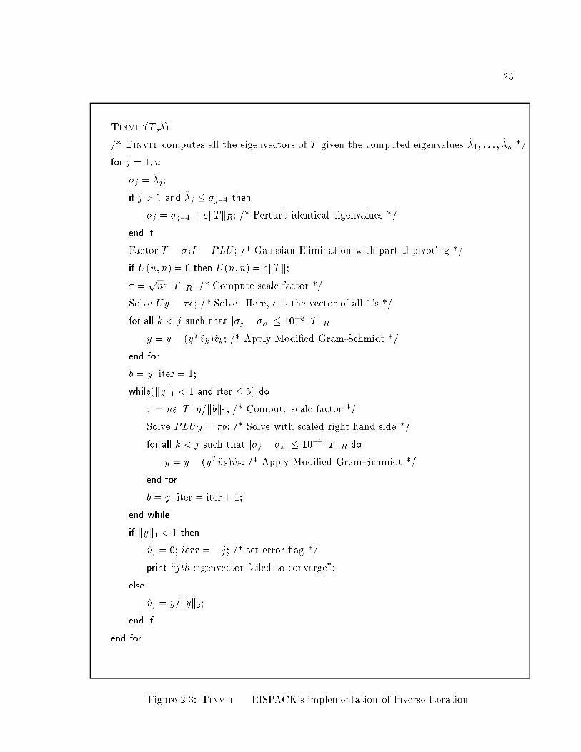
Tinvit(T ,�)
/* Tinvit computes all the eigenvectors of T given the computed eigenvalues �1; : : : ; �n */
for j = 1; n
�j = �j ;
if j > 1 and �j � �j�1 then
�j = �j�1 + "kTkR; /* Perturb identical eigenvalues */
end if
Factor T � �jI = PLU ; /* Gaussian Elimination with partial pivoting */
if U(n; n) = 0 then U(n; n) = "kTk;� =
pn"kTkR; /* Compute scale factor */
Solve Uy = �e; /* Solve. Here, e is the vector of all 1's */
for all k < j such that j�j � �kj � 10�3kTkRy = y � (yT vk)vk; /* Apply Modi�ed Gram-Schmidt */
end for
b = y; iter = 1;
while(kyk1 < 1 and iter � 5) do
� = n"kTkR=kbk1; /* Compute scale factor */Solve PLUy = �b; /* Solve with scaled right hand side */
for all k < j such that j�j � �k j � 10�3kTkR do
y = y � (yT vk)vk; /* Apply Modi�ed Gram-Schmidt */
end for
b = y; iter = iter + 1;
end while
if kyk1 < 1 then
vj = 0; ierr = �j; /* set error ag */print \jth eigenvector failed to converge";
else
vj = y=kyk2;end if
end for
Figure 2.3: Tinvit | EISPACK's implementation of Inverse Iteration
24
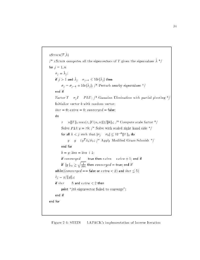
xStein(T ,�)
/* xStein computes all the eigenvectors of T given the eigenvalues � */
for j = 1; n
�j = �j ;
if j > 1 and �j � �j�1 � 10"j�jj then�j = �j�1 + 10"j�jj; /* Perturb nearby eigenvalues */
end if
Factor T � �jI = PLU ; /* Gaussian Elimination with partial pivoting */
Initialize vector b with random vector;
iter = 0; extra = 0; converged = false;
do
� = nkTk1max("; jU(n; n)j)=kbk1; /* Compute scale factor */Solve PLUy = �b; /* Solve with scaled right hand side */
for all k < j such that j�j � �kj � 10�3kTk1 do
y = y � (yT vk)vk; /* Apply Modi�ed Gram-Schmidt */
end for
b = y; iter = iter + 1;
if converged == true then extra = extra + 1; end if
if kyk1 �q
110n
then converged = true; end if
while((converged == false or extra < 2) and iter � 5)
vj = y=kyk2;if iter == 5 and extra < 2 then
print \jth eigenvector failed to converge";
end if
end for
Figure 2.4: STEIN | LAPACK's implementation of Inverse Iteration
25
I. Direction of starting vector. Tinvit chooses the starting vector to be PLe where
T ��I = PLU , � being an approximation to the eigenvalue, and e is the vector of all
1's. Note that this choice of starting vector reduces the �rst iteration to simply solving
Uy = �e. On the other hand, xStein chooses a random starting vector, each of whose
elements comes from a uniform (�1; 1) distribution. Neither choice of starting vectorsis likely to be pathologically de�cient in the desired eigenvector. The random starting
vectors are designed to be superior to Tinvit's choice [87].
II. Choice of shift. Even though in exact arithmetic all the eigenvalues of an unreduced
tridiagonal matrix are distinct, some of the computed eigenvalues may be identical
to working accuracy. In [136, p.329], Wilkinson recommends that pathologically close
eigenvalues be perturbed by a small amount in order to get an orthogonal basis of
the desired subspace. Following this, Tinvit replaces the k+ 1 equal approximations
�j = �j+1 = � � � = �j+k by
�j < �j + "kTkR < � � � < �j + k"kTkR;
where kTkR = maxi jTiij+ jTi;i+1j � kTk1.
We now give an example where this perturbation is too big. As a result, the shifts
used to compute the eigenvectors are quite di�erent from the computed eigenvalues
and prevent the convergence criterion from being attained.
Example 2.8.2 [Excessive Perturbation.] Using LAPACK's test matrix genera-
tor [36], we generated a 200� 200 tridiagonal matrix such that
�1 � � � � � �100 � �"; �101 � � � � � �199 � "; �n = 1
where " � 1:2� 10�7 (this run was in single precision). kTkR = O(1), and the shift
used by Tinvit to compute v199 is
� = �"+ 198"kTkR � 2:3� 10�5:
Since j� � �199j can be as large as
j� � �199j+ j�199� �199j � 4:6� 10�5
the norm growth when solving (2.8.9) is not big enough to meet the convergence
criterion of (2.8.11). Tinvit ags this as an error and returns ierr = �199. tu
26
Clearly, perturbing the computed eigenvalues relative to the norm can substantially
decrease their accuracy. However, not perturbing them is also not acceptable in
Tinvit as coincident shifts would lead to identical L U factors, identical starting
vectors and hence iterates that are parallel to the eigenvectors computed previously !
In xStein, coincident eigenvalues are also perturbed. However, the perturbations
made are relative. Equal approximations �j = �j+1 = � � �= �j+k are replaced by
�j < �j+1 + ��j+1 < � � � < �j+k + ��j+k;
where ��i =P
i�1l=j ��l + 10"j�ij. This choice does not perturb the small eigenval-
ues drastically, and appears to be better than Tinvit's. On the other hand, this
perturbation is too small in some cases to serve its purpose of �nding a linearly in-
dependent basis of the desired subspace (see Example 2.8.7 and Wilkinson's quote
given on page 17). Thus it is easier to say \tweak close eigenvalues" than to �nd a
satisfactory formula for it.
III. Scaling of right hand side and convergence criterion. For each �, the system
(T � �I)y = �b (2.8.9)
is solved in each iteration. With Tinvit's choice of � , the residual norm
k(T � �I)ykkyk =
�kbkkyk =
n"kTkRkyk ; (2.8.10)
where kTkR = maxi jTiij+ jTi;i+1j � kTk1. Tinvit accepts y as an eigenvector if
kyk � 1: (2.8.11)
By (2.8.10), the criterion (2.8.11) ensures that goal (1.1.1) is satis�ed, i.e., k(T ��I)yk=kyk � n"kTkR.
Suppose that in (2.8.9), � is an approximation to �1. Then by analysis similar
to (2.7.6),
kyk = O
�kbkj�1 � �j
!= O
n"kTkRj�1 � �j
!:
Since kyk is expected to be larger than 1 at some iteration, Tinvit requires that �
be such that j�1� �j = O(n"kTk). If the input approximations to the eigenvalues arenot accurate enough, the iterates do not \converge" and Tinvit ags an error.
27
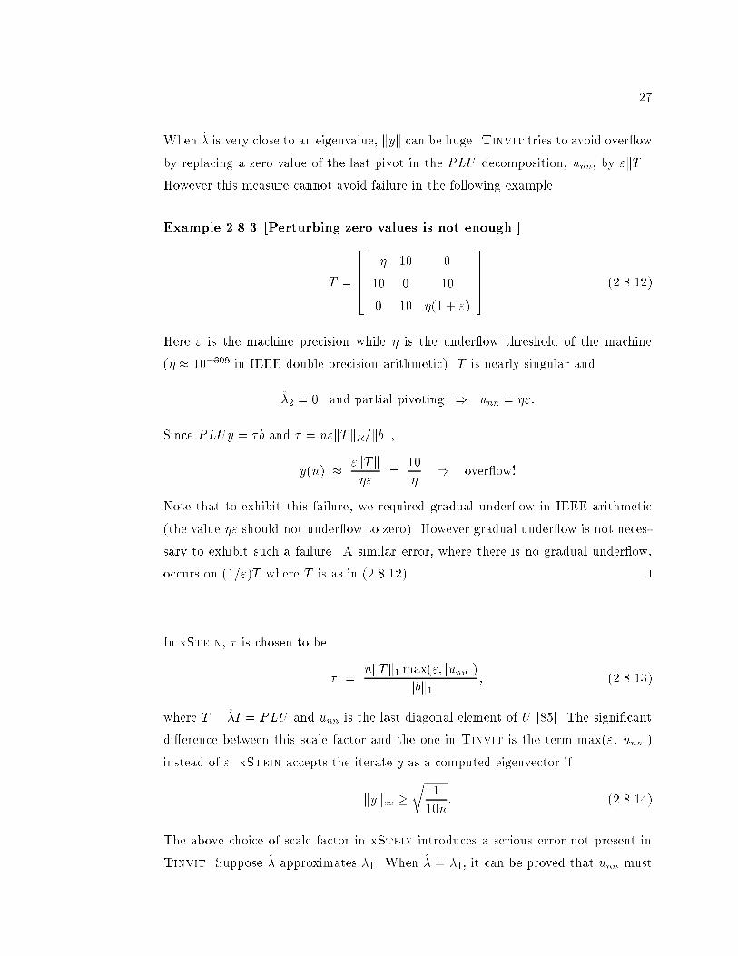
When � is very close to an eigenvalue, kyk can be huge. Tinvit tries to avoid over owby replacing a zero value of the last pivot in the PLU decomposition, unn, by "kTk.However this measure cannot avoid failure in the following example.
Example 2.8.3 [Perturbing zero values is not enough.]
T =
26664�� 10 0
10 0 10
0 10 �(1 + ")
37775 (2.8.12)
Here " is the machine precision while � is the under ow threshold of the machine
(� � 10�308 in IEEE double precision arithmetic). T is nearly singular and
�2 = 0 and partial pivoting ) unn = �":
Since PLUy = �b and � = n"kTkR=kbk,
y(n) � "kTk�"
=10
�) over ow!
Note that to exhibit this failure, we required gradual under ow in IEEE arithmetic
(the value �" should not under ow to zero). However gradual under ow is not neces-
sary to exhibit such a failure. A similar error, where there is no gradual under ow,
occurs on (1=")T where T is as in (2.8.12). tu
In xStein, � is chosen to be
� =nkTk1max("; junnj)
kbk1; (2.8.13)
where T � �I = PLU and unn is the last diagonal element of U [85]. The signi�cant
di�erence between this scale factor and the one in Tinvit is the term max("; junnj)instead of ". xStein accepts the iterate y as a computed eigenvector if
kyk1 �r
1
10n: (2.8.14)
The above choice of scale factor in xStein introduces a serious error not present in
Tinvit. Suppose � approximates �1. When � = �1, it can be proved that unn must
28
be zero in exact arithmetic. We now examine the values unn may take when � 6= �1.
Since T � �I = PLU ,
U�1L�1 = (T � �I)�1P
) eTnU�1L�1en = eT
n(T � �I)�1Pen
Since L is unit lower triangular, L�1en = en. Letting Pen = ek and T = V �V T , we
get
1
unn= eTnV (�� �I)�1V Tek
) 1
unn=
vn1vk1
�1 � �+
nXi=2
vnivki
�i � �; (2.8.15)
where vki denotes the kth component of vi. By examining the above equation, we see
how the choice of scale factor in xStein opens up a Pandora's box. Equation 2.8.15
says that for unn to be small, j�� �1j � jvn1vk1j.
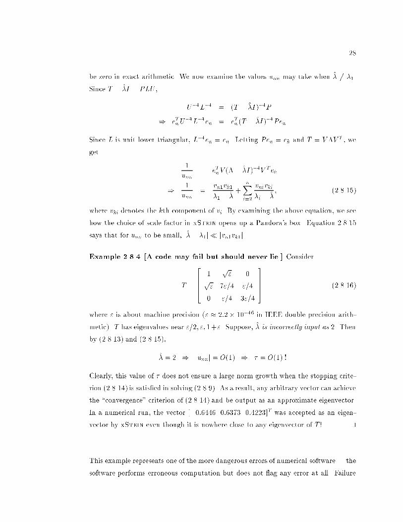
Example 2.8.4 [A code may fail but should never lie.] Consider
T =
26664
1p" 0
p" 7"=4 "=4
0 "=4 3"=4
37775 (2.8.16)
where " is about machine precision (" � 2:2� 10�16 in IEEE double precision arith-
metic). T has eigenvalues near "=2; "; 1+". Suppose, � is incorrectly input as 2. Then
by (2.8.13) and (2.8.15),
� = 2 ) junnj = O(1) ) � = O(1) !
Clearly, this value of � does not ensure a large norm growth when the stopping crite-
rion (2.8.14) is satis�ed in solving (2.8.9). As a result, any arbitrary vector can achieve
the \convergence" criterion of (2.8.14) and be output as an approximate eigenvector.
In a numerical run, the vector [�0:6446 0:6373 0:4223]T was accepted as an eigen-
vector by xStein even though it is nowhere close to any eigenvector of T ! tu
This example represents one of the more dangerous errors of numerical software | the
software performs erroneous computation but does not ag any error at all. Failure
29
to handle incorrect input data can have disastrous consequences 2. On the above
example, Tinvit correctly ags an error indicating that the computation did not
\converge". Of course, most of the times the eigenvalues input to xStein will be
quite accurate and the above phenomenon will not occur.
Even if � is a very good approximation to �1, (2.8.15) indicates that unn may not be
small if vn1 is tiny. It is not at all uncommon for a component of an eigenvector of a
tridiagonal matrix to be tiny [136, pp.317-321]. xStein's choice of scale factor may
lead to unnecessary over ow as shown below.
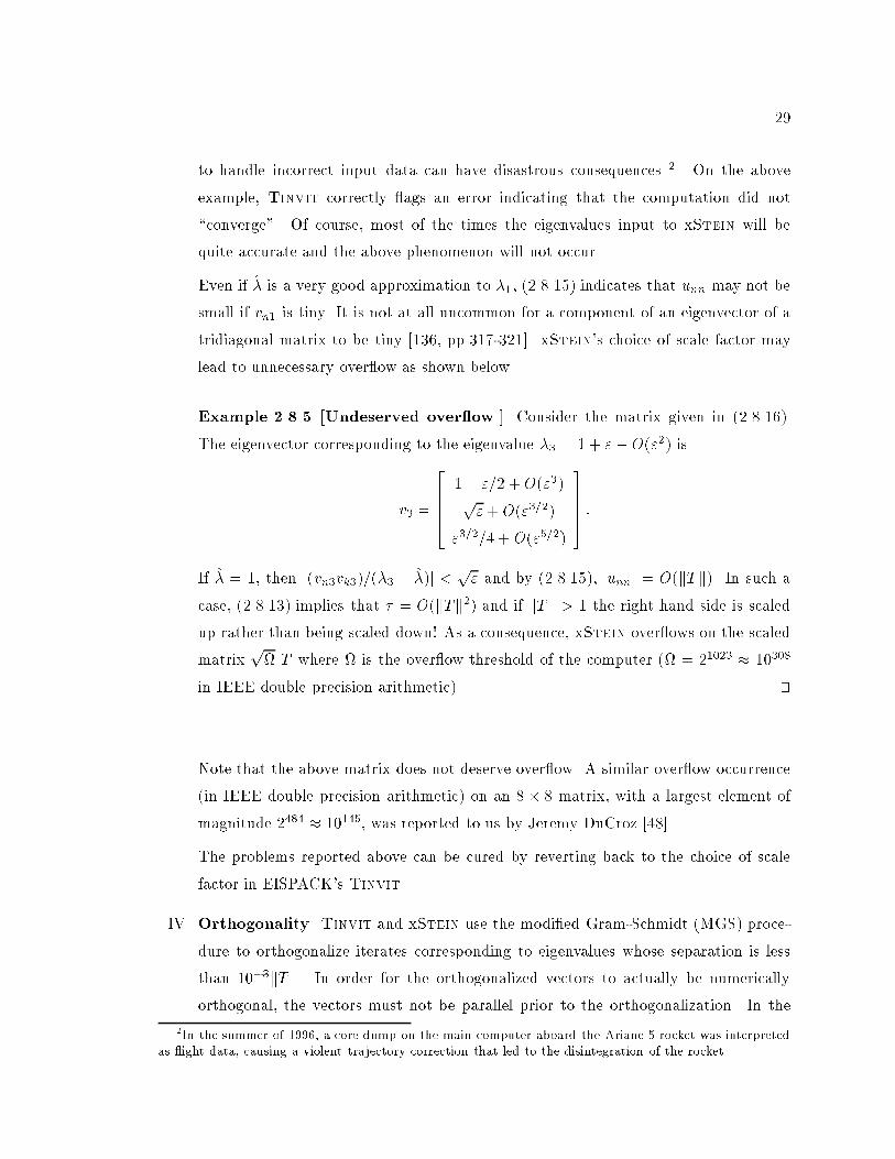
Example 2.8.5 [Undeserved over ow.] Consider the matrix given in (2.8.16).
The eigenvector corresponding to the eigenvalue �3 = 1 + "+O("2) is
v3 =
26664
1� "=2 +O("3)p"+O("3=2)
"3=2=4 + O("5=2)
37775 :
If � = 1, then j(vn3vk3)=(�3 � �)j < p" and by (2.8.15), junnj = O(kTk). In such a
case, (2.8.13) implies that � = O(kTk2) and if kTk > 1 the right hand side is scaled
up rather than being scaled down! As a consequence, xStein over ows on the scaled
matrixp T where is the over ow threshold of the computer ( = 21023 � 10308
in IEEE double precision arithmetic). tu
Note that the above matrix does not deserve over ow. A similar over ow occurrence
(in IEEE double precision arithmetic) on an 8 � 8 matrix, with a largest element of
magnitude 2484 � 10145, was reported to us by Jeremy DuCroz [48].
The problems reported above can be cured by reverting back to the choice of scale
factor in EISPACK's Tinvit.
IV. Orthogonality. Tinvit and xStein use the modi�ed Gram-Schmidt (MGS) proce-
dure to orthogonalize iterates corresponding to eigenvalues whose separation is less
than 10�3kTk. In order for the orthogonalized vectors to actually be numerically
orthogonal, the vectors must not be parallel prior to the orthogonalization. In the
2In the summer of 1996, a core dump on the main computer aboard the Ariane 5 rocket was interpreted
as ight data, causing a violent trajectory correction that led to the disintegration of the rocket
30
following example the vectors to be orthogonalized are almost parallel. The next two
examples are reproduced in Case Study A.
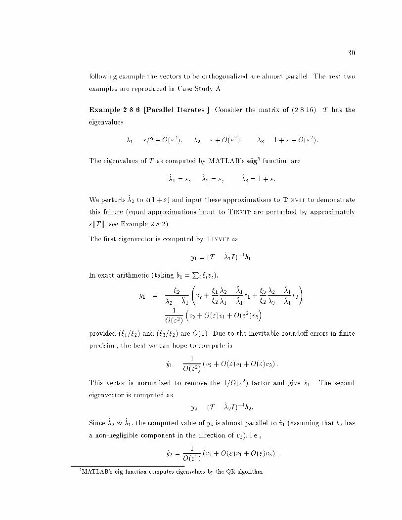
Example 2.8.6 [Parallel Iterates.] Consider the matrix of (2.8.16). T has the
eigenvalues
�1 = "=2 +O("2); �2 = " +O("2); �3 = 1 + "+ O("2):
The eigenvalues of T as computed by MATLAB's eig3 function are
�1 = "; �2 = "; �3 = 1 + ":
We perturb �2 to "(1+ ") and input these approximations to Tinvit to demonstrate
this failure (equal approximations input to Tinvit are perturbed by approximately
"kTk, see Example 2.8.2).
The �rst eigenvector is computed by Tinvit as
y1 = (T � �1I)�1b1:
In exact arithmetic (taking b1 =P
i�ivi),
y1 =�2
�2 � �1
v2 +
�1
�2
�2 � �1
�1 � �1v1 +
�3
�2
�2 � �1
�3 � �1v3
!
=1
O("2)
�v2 + O(")v1 +O("2)v3
�
provided (�1=�2) and (�3=�2) are O(1). Due to the inevitable roundo� errors in �nite
precision, the best we can hope to compute is
y1 =1
O("2)(v2 + O(")v1 +O(")v3) :
This vector is normalized to remove the 1=O("2) factor and give v1. The second
eigenvector is computed as
y2 = (T � �2I)�1b2:
Since �2 � �1, the computed value of y2 is almost parallel to v1 (assuming that b2 has
a non-negligible component in the direction of v2), i.e.,
y2 =1
O("2)(v2 + O(")v1 +O(")v3) :
3MATLAB's eig function computes eigenvalues by the QR algorithm
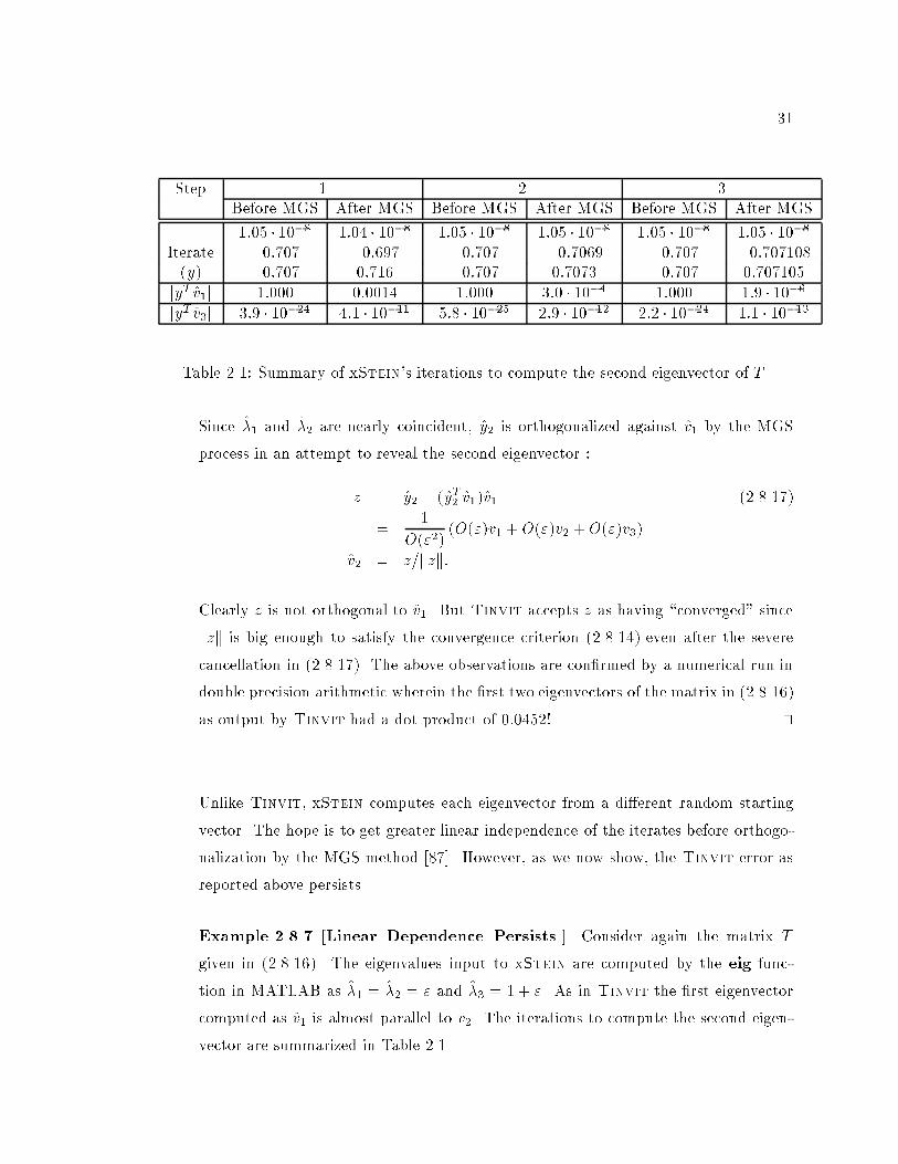
31
Step 1 2 3
Before MGS After MGS Before MGS After MGS Before MGS After MGS
1:05 � 10�8 1:04 � 10�8 1:05 � 10�8 1:05 � 10�8 1:05 � 10�8 1:05 � 10�8Iterate �0:707 �0:697 �0:707 �0:7069 �0:707 �0:707108(y) �0:707 0:716 �0:707 0:7073 �0:707 0:707105
jyT v1j 1:000 0:0014 1:000 3:0 � 10�4 1:000 1:9 � 10�6jyT v3j 3:9 � 10�24 4:1 � 10�11 5:8 � 10�25 2:9 � 10�12 2:2 � 10�24 1:1 � 10�13
Table 2.1: Summary of xStein's iterations to compute the second eigenvector of T .
Since �1 and �2 are nearly coincident, y2 is orthogonalized against v1 by the MGS
process in an attempt to reveal the second eigenvector :
z = y2 � (yT2 v1)v1 (2.8.17)
=1
O("2)(O(")v1 + O(")v2 + O(")v3)
v2 = z=kzk:
Clearly z is not orthogonal to v1. But Tinvit accepts z as having \converged" since
kzk is big enough to satisfy the convergence criterion (2.8.14) even after the severe
cancellation in (2.8.17). The above observations are con�rmed by a numerical run in
double precision arithmetic wherein the �rst two eigenvectors of the matrix in (2.8.16)
as output by Tinvit had a dot product of 0:0452! tu
Unlike Tinvit, xStein computes each eigenvector from a di�erent random starting
vector. The hope is to get greater linear independence of the iterates before orthogo-
nalization by the MGS method [87]. However, as we now show, the Tinvit error as
reported above persists.
Example 2.8.7 [Linear Dependence Persists.] Consider again the matrix T
given in (2.8.16). The eigenvalues input to xStein are computed by the eig func-
tion in MATLAB as �1 = �2 = " and �3 = 1 + ". As in Tinvit the �rst eigenvector
computed as v1 is almost parallel to v2. The iterations to compute the second eigen-
vector are summarized in Table 2.1.
32
This behavior is very similar to that of Tinvit (see Example 2.8.6). xStein does two
more iterations than Tinvit and alleviates the problem slightly, but a dot product
of 1:9� 10�6 between computed eigenvectors is far from satisfactory (this run was in
double precision). tu
xStein avoids the over ow problems of Tinvit shown in example 2.8.3. It checks
to see if over ow would occur, and if so, perturbs tiny entries on the diagonal of U [85]. This
check is in the inner loop when solving Uy = x where x = �L�1P�1b. Coupled with the
extra iterations done after convergence, this results in xStein being slower than Tinvit.
On an assorted collection of test matrices of sizes 50 to 1000, we observed xStein to be 2-3
times slower than Tinvit. However xStein was more accurate than Tinvit in general.
2.9 Our Approach
As we observed in the previous section, the computer implementation of a seem-
ingly straightforward task can lead to surprising failures. We want to avoid such failures
and indicate our approach to the various aspects of inverse iteration discussed above.
I. Choice of shift. Of the various issues discussed in Section 2.7, the choice of starting
vector and convergence criterion have been extensively studied [136, 118, 119, 87].
Surprisingly, the choice of shift for inverse iteration seems to have drawn little at-
tention. We feel that the shift is probably the most important variable in inverse
iteration. Examples 2.8.6 and 2.8.7 highlight the importance of shifts that are as
accurate as possible. We present our solution in Chapter 4.
II. Direction of starting vector and scaling of right hand side. This problem is
solved. It is now possible to deterministically �nd a starting vector that is guaranteed
to have an above average component in the direction of the desired eigenvector v.
Knowing the position of a large component of v also enables us to avoid the possibility
of over ow in the eigenvector computation. See Chapter 3 for more details.
III. Convergence criterion and Orthogonality. It is easy to �nd a criterion that
guarantees small residual norms (goal (1.1.1)). However, as we saw in earlier sections,
the goal of orthogonality (1.1.2) can lead to a myriad of problems. Most of the \di�-
cult" errors in the EISPACK and LAPACK implementations arise due to the explicit
33
orthogonalization of iterates when eigenvalues are close. In [20], Chandrasekaran ex-
plains the theory behind some of these failures, and proposes an alternate version
of inverse iteration that is provably correct. However, this version is more involved
and potentially requires much more orthogonalization than in existing implementa-
tions. We want to take a di�erent approach to orthogonality, and this is discussed in
Chapters 4, 5 and 6.
34
Chapter 3
Computing the eigenvector of an
isolated eigenvalue
Given an eigenvalue � of a tridiagonal matrix ~J , a natural way to solve for v 6= 0
in
( ~J � �I)v = 0 (3.0.1)
is to set v(1) = 1 and to use the �rst equation of (3.0.1) to determine v(2), and the second
to determine v(3), using v(1) and v(2). Proceeding like this, the rth equation may be used
to determine v(r+ 1) and thus v may be obtained without actually making use of the nth
equation which will be satis�ed automatically since the system (3.0.1) is singular.
It would be equally valid to begin with ~v(n) = 1 and to take the equations in
reverse order to compute ~v(n � 1); : : : ; ~v(2); ~v(1) in turn without using the �rst equation
in (3.0.1). When normalized in the same way v and ~v will yield the same eigenvector in
exact arithmetic.
The method described above is `obvious' and was mentioned by W. Givens in
1957, see [61]. It often gives good results when realized on a computer but, at other times,
delivers vectors pointing in completely wrong directions for the following reason. It is
rare that an eigenvalue of a tridiagonal (or any other) matrix is representable in limited
precision. Consequently the systems such as (3.0.1) that are to be solved are not singular
and, in (3.0.1), the unused equation will not be satis�ed automatically even if the solutions
of the other equations were obtained exactly. The two methods given above result in solving
( ~J � �I)x(n) = �nen (3.0.2)
35
and
( ~J � �I)x(1) = �1e1 (3.0.3)
respectively, where � is an approximation to � and �1, �n are the residuals of the equations
that are not satis�ed. Note that (3.0.2) and (3.0.3) show that the natural method may be
thought of as doing one step of inverse iteration as given in (2.7.4) with the starting vector
equal to e1 or en. We now present an example illustrating how this natural method can
fail.
Example 3.0.1 [Choice of e1 is wrong.] Consider
T =
266643"=4 "=4 0
"=4 7"=4p"
0p" 1
37775 (3.0.4)
where " is of the order of the machine precision. An eigenvalue of T is
� = 1+ "+ O("2);
and its associated eigenvector is
v =
26664"3=2=4 + O("5=2)p"+ O("3=2)
1� "=2 +O("2)
37775 : (3.0.5)
The vector obtained in exact arithmetic by ignoring the �rst equation, with the approxi-
mation � = 1, is
x(1) =
26664�4=p"
0
1
37775 ;
butk(T � �I)x(1)k2
kx(1)k2=
4� 3"p16 + "
! 1 as "! 0:
tu
In [136, pp.319{321] and[134], Wilkinson presents a similar example where omit-
ting the last equation results in a poor approximation to an eigenvector. His example matrix
36
is
W�
21 =
26666666666666664
10 1 0
1 9 1
1 8 :
: : :
: �8 1
1 �9 1
0 1 �10
37777777777777775
: (3.0.6)
Letting � be the largest eigenvalue of W�
21, Wilkinson shows that there is no 9-�gure ap-
proximation � to � for which the exact normalized solution of the �rst 20 equations of
(W�
21 � �I)x = 0 is anywhere close to the desired eigenvector. We now repeat his analysis.
Suppose
( ~J � �I)x(r) = er ;
where � approximates �j . Writing er in terms of the eigenvectors, er =P
n
i=1 �ivi, we get
x(r) = ( ~J � �I)�1er
=�j
�j � �
0@vj +X
i6=j
�i
�j
�j � �
�i � �vi
1A (3.0.7)
Fundamental limitations of �nite precision arithmetic dictate that j�� �j j cannot be bet-ter than O(n"k ~Jk), in general, where " is the machine precision. Even when j� � �jj �n"k ~Jk, (3.0.7) shows that x(r) may not be close to vj 's direction if �j = e�
rvj = vj(r) is tiny.
In Example 3.0.1, r = 1 and �j � O("3=2) while in Wilkinson's example, r = n = 21 and
�j = 10�17. As a result, in both these cases the natural method does not approximate the
eigenvector well.
Given an accurate �, (3.0.7) implies that x(r) will be a good approximation to vj
provided the rth component of vj is not small. Wilkinson notes this in [136, p.318] and
concludes,
`Hence if the largest component of uk [vj in our notation] is the rth, then it
is the rth equation which should be omitted when computing uk. This result
is instructive but not particularly useful, since we will not know a priori the
position of the largest component of uk . In fact, uk is precisely what we are
attempting to compute!'
In the absence of a reliable and cheap procedure to �nd r, Wilkinson compromised
by choosing the starting vector for inverse iteration as PLe, where ~J � �I = PLU and e
37
is the vector of all 1's (this led to the choice made in EISPACK [128]). A random starting
vector is used in the LAPACK implementation of inverse iteration [87].
In this chapter, we show the following
1. Sections 3.1 and 3.2 introduce twisted factorizations that provide an answer to Wilkin-
son's problem of choosing which equation to omit. This is due to pioneering work by
Fernando, and enables us to discard LAPACK's random choice of starting vector to
compute an eigenvector of an isolated eigenvalue [57, 117].
2. In Section 3.3 we show how to adapt the results of Sections 3.1 and 3.2 when triangular
factorizations don't exist. Some of the material presented in Sections 3.1-3.3 has
appeared in [117].
3. Section 3.4 shows how to eliminate the divisions in the method outlined in Section 3.2.
4. In Section 3.5, we introduce twisted Q factorizations and give an alternate method
to compute an eigenvector. We also show how the perfect shift strategy suggested by
Parlett [110, p.173] can be made to succeed.
5. In Section 3.6, we show that twisted factorizations may also be used to detect singu-
larity of Hessenberg and dense matrices.
In preparation for the upcoming theory, we state a few well known results without
proof. The informed reader should be able to furnish their proofs without much di�culty.
We expect that the reader knows the LDU decomposition and theorem concerning existence
and uniqueness of triangular factorization and the expressions for the pivots, as the diagonal
entries of D are often called.
Lemma 3.0.1 Let ~J be an unreduced tridiagonal matrix and v be an eigenvector. Then the
�rst and last components of v are non-zero.
Lemma 3.0.2 Let ~J be an unreduced normal tridiagonal matrix. Then every eigenvalue of
~J is simple.
Lemma 3.0.3 Let J = ~J � �I be an unreduced singular tridiagonal matrix where � is an
eigenvalue of ~J and v is the corresponding eigenvector. Then the following are equivalent.
i. J admits the LDU and UDL triangular factorizations.
38
ii. All strictly leading and trailing submatrices of J are nonsingular.
Furthermore when J is normal, the following is equivalent to the above
iii. No component of v is zero.
Proof. The latter is not so obvious and follows from the fact that when J is normal
jv(i)j2�0(�) = �1:i�1(�) � �i+1:n(�) (3.0.8)
where �l:m(�) = det(�I � ~J l:m). See [110, Section 7-9] to derive the above. tu
3.1 Twisted Factorizations
Despite Wilkinson's pessimism, we ask the question: can we �nd reliable indica-
tors of the sizes of various components of a normalized eigenvector without knowing the
eigenvector itself? We turn to triangular factorization in search of an answer and examine
the LDU decomposition of ~J � �I . In this representation, both L and U have 1's on the
diagonal. We will denote the ith diagonal element of D by D(i) and L(i+ 1; i); U(i; i+ 1)
by L(i) and U(i) respectively.
If � is an eigenvalue of ~J , the following theorem implies that D(n) must be zero
in exact arithmetic.
Theorem 3.1.1 Let B be a matrix of order n such that the triangular factorization
B = LDU
exists, i.e., its principal submatrices B1:i, i = 1; 2; : : : ; n� 1 are nonsingular. Then if B is
singular,
D(n) = 0:
Proof. The expression
D(n) =det(B)
det(B1:n�1)
implies that if B is singular, D(n) = 0. tuWe now examine the values D(n) can take when � is not an eigenvalue. Suppose
� approximates �j . Since ~J � �I = LDU ,
U�1D�1L�1 = ( ~J � �I)�1
) e�nU�1D�1L�1en = e�n(
~J � �I)�1en
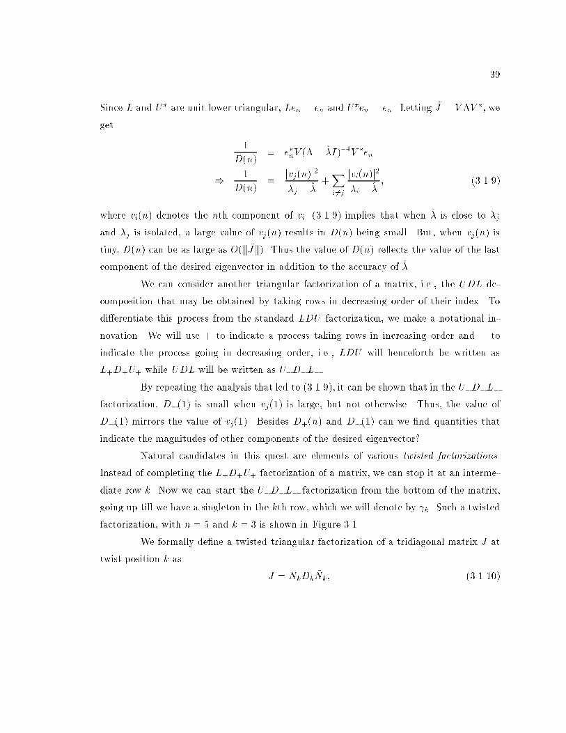
39
Since L and U� are unit lower triangular, Len = en and U�en = en. Letting ~J = V �V �, we
get
1
D(n)= e�
nV (�� �I)�1V �en
) 1
D(n)=
jvj(n)j2
�j � �+Xi6=j
jvi(n)j2�i � �
; (3.1.9)
where vi(n) denotes the nth component of vi. (3.1.9) implies that when � is close to �j
and �j is isolated, a large value of vj(n) results in D(n) being small. But, when vj(n) is
tiny, D(n) can be as large as O(k ~Jk). Thus the value of D(n) re ects the value of the last
component of the desired eigenvector in addition to the accuracy of �.
We can consider another triangular factorization of a matrix, i.e., the UDL de-
composition that may be obtained by taking rows in decreasing order of their index. To
di�erentiate this process from the standard LDU factorization, we make a notational in-
novation. We will use + to indicate a process taking rows in increasing order and � to
indicate the process going in decreasing order, i.e., LDU will henceforth be written as
L+D+U+ while UDL will be written as U�D�L�.
By repeating the analysis that led to (3.1.9), it can be shown that in the U�D�L�
factorization, D�(1) is small when vj(1) is large, but not otherwise. Thus, the value of
D�(1) mirrors the value of vj(1). Besides D+(n) and D�(1) can we �nd quantities that
indicate the magnitudes of other components of the desired eigenvector?
Natural candidates in this quest are elements of various twisted factorizations.
Instead of completing the L+D+U+ factorization of a matrix, we can stop it at an interme-
diate row k. Now we can start the U�D�L� factorization from the bottom of the matrix,
going up till we have a singleton in the kth row, which we will denote by k. Such a twisted
factorization, with n = 5 and k = 3 is shown in Figure 3.1.
We formally de�ne a twisted triangular factorization of a tridiagonal matrix J at
twist position k as
J = NkDk~Nk; (3.1.10)
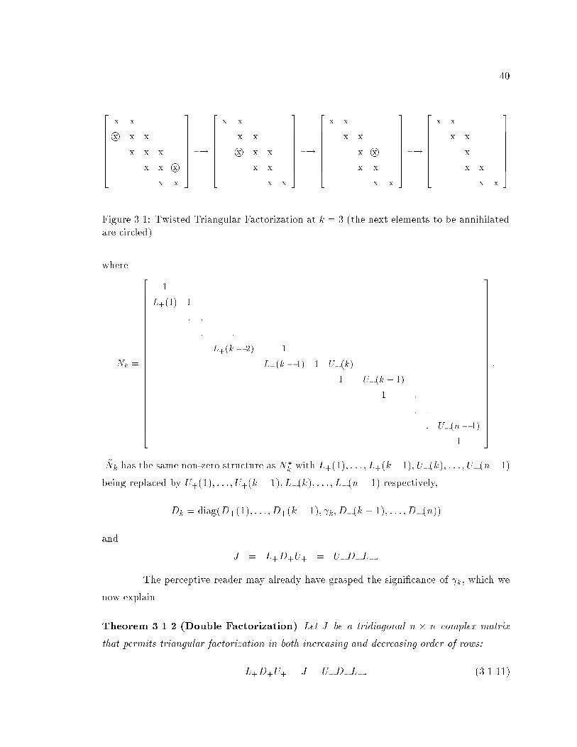
40
266666664
x x
x x x
x x x
x x x
x x
377777775�!
266666664
x x
x x
x x x
x x
x x
377777775�!
266666664
x x
x x
x x
x x
x x
377777775�!
266666664
x x
x x
x
x x
x x
377777775
Figure 3.1: Twisted Triangular Factorization at k = 3 (the next elements to be annihilated
are circled)
where
Nk =
26666666666666666666666664
1
L+(1) 1
: :
: :
L+(k � 2) 1
L+(k � 1) 1 U�
(k)
1 U�
(k + 1)
1 :
: :
: U�
(n� 1)
1
37777777777777777777777775
;
~Nk has the same non-zero structure as N�
kwith L+(1); : : : ; L+(k�1); U�(k); : : : ; U�(n�1)
being replaced by U+(1); : : : ; U+(k � 1); L�(k); : : : ; L�(n� 1) respectively,
Dk = diag(D+(1); : : : ; D+(k � 1); k; D�(k + 1); : : : ; D�(n))
and
J = L+D+U+ = U�D�L�:
The perceptive reader may already have grasped the signi�cance of k, which we
now explain.
Theorem 3.1.2 (Double Factorization) Let J be a tridiagonal n � n complex matrix
that permits triangular factorization in both increasing and decreasing order of rows:
L+D+U+ = J = U�D�L�: (3.1.11)
41
Consider the twisted factorization at k given by (3.1.10). Then for 1 � k � n,
k = D+(k) +D�(k)� Jkk (3.1.12)
and if J is invertible,1
k= e�
kJ�1ek: (3.1.13)
Proof. By construction of the twisted factorization,
k = �Jk�1;kL+(k � 1) + Jkk � Jk+1;kU�(k) (3.1.14)
= (Jkk � Jk�1;kL+(k � 1))� Jkk + (Jkk � Jk+1;kU�(k))
= D+(k)� Jkk +D�(k)
for 1 � k � n. Here we take J1;0 = J0;1 = Jn+1;n = Jn;n+1 = 0, and L+(0) = U�(n) = 0.
Since Nkek = ek and e�k~Nk = e�
k,
e�kJ�1ek = e�k
~N�1kD�1
kN�1kek
=1
k
tuNote that n = D+(n) and 1 = D�(1). The above theorem shows how to get all
possible n twisted factorizations at the cost of 2n divisions. The alert reader would have
noted that the above theorem makes no assumption about the nearness to singularity of J .
We want to emphasize that in the theory developed here the existence of the tri-
angular factorizations (3.1.11) is not restrictive. Neither is the occasional requirement that
J be nonsingular. In fact, the singularity of J is desirable in our application of computing
an eigenvector. As we will show in Section 3.3, in the absence of these requirements, all
the theory developed in this section and the next is easily extended if 1 is added to the
number system.
The following corollary gives alternate expressions for k.
42
Corollary 3.1.1 With the notation of Theorem 3.1.2, for 1 < k < n,
k =
8>>>>>>>>>>>>>>>>>>>>>><>>>>>>>>>>>>>>>>>>>>>>:
D+(k)� Jkk +D�(k);
�Jk�1;kL+(k � 1) + Jkk � Jk+1;kU�(k);
�Jk;k�1U+(k � 1) + Jkk � Jk;k+1L�(k);
D+(k)� Jk+1;kU�(k);
�Jk�1;kL+(k � 1) +D�(k):
For k = 1 and k = n omit terms with invalid indices.
Proof. The �rst and second expressions are just (3.1.12) and (3.1.14). The others come
from rewriting (3.1.14) as
k = �Jk;k�1Jk�1;k=D+(k � 1) + Jkk � Jk;k+1Jk+1;k=D�(k + 1) (3.1.15)
and using Jk;k+1 = U�(k)D�(k+ 1) = D+(k)U+(k) etc., and the formula for the backward
pivots, D�(k) = Jkk � Jk;k+1Jk+1;k=D�(k+ 1), etc. tuAs shown below, double factorization makes available the so called Newton correction.
Corollary 3.1.2 Assume the hypothesis (3.1.11) of Theorem 3.1.2, and let J be nonsingu-
lar. ThennXi=1
�1i
= Trace(J�1) = � �0(0)
�(0); (3.1.16)
where �(�) = det(�I � J).
Proof. By (3.1.13) in Theorem 3.1.2,
Xi
�1i
=Xi
e�i J�1ei = Trace(J�1) = � �0(0)
�(0)
since�0(�)
�(�)=
Pj
Qi6=j(� � �i)Qi(�� �i)
=Xi
1
�� �i:
tuDouble factorization also allows a wide choice of expressions for det(J), and a recurrence
for computing i that involves only multiplications and divisions.
43
Theorem 3.1.3 Assume the hypothesis of Theorem 3.1.2. Then for k = 1; : : : ; n (omit
invalid indices),
det(J) = D+(1) � � �D+(k � 1) kD�(k + 1) � � �D�(n) (3.1.17)
and
kD�(k + 1) = D+(k) k+1: (3.1.18)
Proof. From (3.1.10),
det(J) = det(Nk) det(Dk) det( ~Nk) = det(Dk);
and we get (3.1.17). Applying (3.1.17) to two successive k's leads to (3.1.18). tuThe following are immediate consequences of (3.1.17),
Corollary 3.1.3 Assuming the hypothesis of Theorem 3.1.2,
k = D+(k)nY
i=k+1
(D+(i)=D�(i));
= D�(k)k�1Yi=1
(D�(i)=D+(i)):
Corollary 3.1.4 Assuming the existence of the twisted factorization (3.1.10),
k =det(J)
det(J1:k�1) det(Jk+1:n):
Note that the above corollary shows that k = 0 if J is singular and admits triangular
factorizations (3.1.11). See also Theorem 3.1.1 which proves that n = 0 when J is singular.
The Double Factorization theorem is not new. In 1992, in [108], Meurant reviewed
a signi�cant portion of the literature on the inverses of band matrices and presented the
main ideas in a nice uni�ed framework. The inexpensive additive formulae for (J�1)kk
(Theorem 3.1.2 and Corollary 3.1.1) are included in Theorem 3.1 of [108], while our Corol-
lary 3.1.3 that gives the quotient/product form of (J�1)kk is given in Theorem 2.3 of [108].
We believe that such formulae have been known for quite some time in the di�erential
equations community. However, these researchers were not interested in computing eigen-
vectors but in obtaining analytic expressions for elements of the inverse, when possible,
and in the decay rate in terms of distance from the main diagonal. Our contribution is
in recognizing the importance of twisted factorizations and successfully applying them to
44
solve some elusive problems in numerical linear algebra. We will show some of these ap-
plications in this thesis, for other applications see [42, 115, 74]. In addition to the papers
reviewed in [108], twisted factorizations have appeared in various contexts in the literature,
see [77, 94, 5, 58, 130, 133, 44]. For a brief review, see Section 4.1 of [117]. Twisted factor-
izations have also been referred to as BABE factorizations (Begin, or Burn, at Both Ends)
in [78, 57, 74].
3.2 The Eigenvector Connection
Given an eigenvalue approximation � of ~J , we can compute the double factorization
of ~J � �I by Theorem 3.1.2. In this section, we see how double factorization can be used to
�nd a \good" equation to omit when solving the system ( ~J � �I)x = 0, thereby obtaining
a good approximation to the desired eigenvector. Some of the results of this section have
appeared in [117].
Since �1k
= e�k( ~J � �I)�1ek , if we let ~J = V �V �, we get an expression for k that
is similar to (3.1.9),
1
k= e�kV (�� �I)�1V �ek;
) 1
k=
jvj(k)j2
�j � �+Xi6=j
jvi(k)j2
�i � �: (3.2.19)
Thus when � is close to an isolated �j and �j is isolated, the value of k re ects the value
of vj(k), i.e, an above average value of vj(k) leads to a tiny value of k while a small vj(k)
implies a large k. We now make this claim more precise.
Lemma 3.2.1 Let ~J � �I be a normal, unreduced nonsingular tridiagonal matrix that sat-
is�es the hypotheses of Theorem 3.1.2 for all � in some open interval containing the eigen-
value �j. Let k = k(�) be as in (3.1.13), for each k. As � �! �j,
�1kP
n
m=1 �1m
�! jvj(k)j2; k = 1; 2; : : : ; n: (3.2.20)
Proof. For � 6= �j ,
�~J � �I
��1
= V (�� �I)�1V � =Xi
viv�
i (�i � �)�1:
45
From (3.1.13) in Theorem 3.1.2, �1k
=
��~J � �I
��1�kk
. Since �j is simple by Lemma 3.0.2,
as � �! �j,
(�j � �)�~J � �I
��1
�! vjv�
j;
(�j � �) �1k
�! jvj(k)j2; k = 1; 2; : : : ; n
(�j � �)nX
m=1
�1m
�! kvjk2 = 1:
tuThe following theorem replaces the limits of Lemma 3.2.1 with error bounds. It
implies that when � is su�ciently close to �j then one of the k's must be small. Note that
in the following theorem, the matrix need not be tridiagonal and the eigenvalues may be
complex.
Theorem 3.2.1 Let ~J � �I be a normal, invertible matrix, and let
�1k
= e�k(~J � �I)�1ek ; for k = 1; 2; : : : ; n:
Then if vj(k) 6= 0,
k =�j � �
jvj(k)j2h1 +
�jvj(k)j�2 � 1
�A1
i�1
: (3.2.21)
Here A1 is a weighted arithmetic mean ofn�j��
�i��; i 6= j
o, 0 � jA1j < j�j��j=gap(�), where
gap(�) = mini6=j j�i � �j. Furthermore, if �j is isolated enough, i.e.,
j�j � �jgap(�)
� 1
M� 1
n � 1where M > 1 (3.2.22)
then for k such that jvj(k)j � 1=pn,
j kj � j�j � �jjvj(k)j2
� M
M � 1� nj�j � �j � M
M � 1(3.2.23)
Proof.
�1k
= e�k( ~J � �I)�1ek;
=nXi=1
jvi(k)j2�i � �
:
Extract the jth term to �nd
�1k
=
jvj(k)j2�j � �
!241 +X
i6=j
����� vi(k)vj(k)
�����2 �
�j � �
�i � �
�35 : (3.2.24)
46
Since Xi6=j
����� vi(k)vj(k)
�����2
=1� jvj(k)j2jvj(k)j2
theP
i6=j term in (3.2.24) may be written as
�jvj(k)j�2 � 1
�A1; jA1j � j�j � �j=gap(�);
where
A1 =Xi6=j
wi
��j � �
�i � �
�; 1 =
Xi6=j
wi; wi � 0; gap(�) = mini6=j
j�i � �j;
to yield the equality in (3.2.21). If (3.2.22) holds, then
j kj � j�j � �jjvj(k)j2
�1�
�jvj(k)j�2 � 1
�� 1
M � (n� 1)
���1
:
For k such that jvj(k)j � 1=pn,
j kj � j�j � �jjvj(k)j2
�1� 1
M
��1
:
tuIn cases of interest, j�j ��j=gap(�) = O(") and hence M � 1. Thus the factor M=(M � 1)
in (3.2.23) is � 1.
The following theorem shows a way to compute the vector z that satis�es all the
equations of ( ~J � �I)z = 0 except the kth.
Theorem 3.2.2 Let J = ~J��I be an unreduced tridiagonal matrix that permits the twisted
factorization (3.1.10) for a �xed value of k. Then the system
( ~J � �I)z(k) = kek (3.2.25)
has a unique solution given by
z(k)(k) = 1;
z(k)(j) = �U+j;j+1z
(k)(j + 1); j = k � 1; : : : ; 1;
z(k)(i) = �L�i;i�1z
(k)(i� 1); i = k + 1; : : : ; n:
Proof. Since Nkek = ek and Dkek = kek,
( ~J � �I)z(k) = kek ) ~Nkz(k) = ek
47
from which the result follows. tuNote that when J is unreduced, the above theorem precludes z(k) from having a zero entry.
This is consistent with Theorem 3.0.3. A bene�t of computing z(k) is the availability of the
Rayleigh Quotient.
Corollary 3.2.1 Let ~J � �I satisfy the hypothesis of Theorem 3.1.2, and z = z(k) be as
in (3.2.25) for 1 � k � n. Then the Rayleigh Quotient of z is given by
z� ~Jz
z�z= � +
k
kzk2 (3.2.26)
Proof. By (3.2.25),
z�( ~J � �I)z = kz�ek = k
since z(k) = 1. The result (3.2.26) follows. tuSince kz(k)k � 1, Theorem 3.2.1 implies that the residual norm
k( ~J � �I)z(k)kkz(k)k =
j kjkz(k)k (3.2.27)
is small when � is a good approximation to an isolated eigenvalue �, and k is chosen
appropriately. The following theorem gives a better bound on mink j kj=kz(k)k.
Theorem 3.2.3 Let ~J � �I be a normal, invertible matrix, and let
( ~J � �I)z(k) = ek k; for k = 1; 2; : : : ; n:
Then if vj(k) 6= 0,
j kjkz(k)k =
j� � �j jjvj(k)j
h1 +
�jvj(k)j�2 � 1
�A2
i�1=2
;
� j� � �j jjvj(k)j
�pn j�� �j j for at least one k: (3.2.28)
Here A2 is a weighted arithmetic mean of
�������j
���i
���2 ; i 6= j
�, 0 < A2 < [j�j � �j=gap(�)]2.
Proof.
z(k) = ( ~J � �I)�1ek k;
kz(k)k2 = j kj2e�kV (��� ��I)�1(�� �I)�1V �ek
= j kj2nXi=1
jvi(k)j2j�� �ij2
:
48
Extract the jth term to �nd
kz(k)kj kj
!2
=
jvj(k)jj�� �j j
!2241 +X
i6=j
����� vi(k)vj(k)
�����2 ������ �j
�� �i
����235
) j kjkz(k)k =
j�� �j jjvj(k)j
h1 +
�jvj(k)j�2 � 1
�A2
i�1=2
;
where
A2 =Xi6=j
wi
������ �j
� � �i
����2
; 1 =Xi6=j
wi; wi � 0; 0 < A2 < [j�j � �j=gap(�)]2:
Since (jvj(k)j�2 � 1)A2 � 0, (3.2.28) follows easily from the above. tuThe above theorems suggest a way to compute a vector z(k) such that the residual
norm (3.2.27) is small. In 1995, Fernando, in an equivalent formulation, proposed choosing
the index for which j kj is minimum, say r, and then solving ( ~J��I)z(r) = rer to compute
an approximate eigenvector z(r). See [57] for his subsequent work. Earlier, in 1985, Godunov
and his collaborates proposed a similar but more obscure method for obtaining a provably
accurate approximation to an eigenvector by `sewing' together two \Sturm Sequences" that
start at either end of the matrix. See [64] and [63] for their work, and Section 4.2 of [117]
for interpretation in our notation. Fernando's approach leads to the following algorithm
Algorithm 3.2.1 [Computing an eigenvector of an isolated eigenvalue.]
1. Compute ~J � �I = L+D+U+ = U�D�L�.
2. Compute k for k = 1; 2; : : : ; n using the expressions in Corollary 3.1.1 or (3.1.18) in
Theorem 3.1.3 and choose the index r where j kj is minimum.
3. Form the vector z(r) as in Theorem 3.2.2.
tu
Note that z(r) is formed by multiplications only, thus promising greater accuracy
and a more favorable error analysis than standard methods that involve additions. Us-
ing (3.2.23) and the fact that kz(r)k � 1, the above algorithm bounds the residual norm
by
k( ~J � �I)z(r)kkz(r)k � nj�j � �j � M
M � 1: (3.2.29)
49
This solves Wilkinson's problem of choosing which equation to omit, modulo the mild
assumption (3.2.22) about the separation of �j . As we shall emphasize in later chapters,
we will use Algorithm 3.2.1 only when �j is su�ciently isolated.
We have noted, and so has Jessie Barlow [8], that a simple recurrence will yield
all values of kz(k)k for O(n) operations. Consequently it would be feasible to minimize
j kj=kz(k)k instead of j kj to obtain a possibly smaller residual norm. At present we feel
that the extra expense is not warranted. The bound given by (3.2.28) is certainly better
than the above bound (3.2.29). However, the latter bound is much too pessimistic since
kz(r)k can be as large aspn when all eigenvector entries are equal in magnitude.
3.3 Zero Pivots
We now show that the procedure to compute an eigenvector suggested by the
previous section needs to be modi�ed only slightly when J = ~J � �I does not admit
the triangular factorizations (3.1.11) in Theorem 3.1.2. We will continue to assume exact
arithmetic | the e�ect of roundo� errors in a computer implementation is examined in the
next chapter.
Triangular factorization is said to fail, or not exist, if a zero `pivot', D+(j) or
D�(j) is encountered prematurely. The last pivot is allowed to vanish because it does not
occur as a denominator in the computation.
One of the attractions of an unreduced tridiagonal matrix is that the damage
done by a zero pivot is localized. Indeed, if �1 is added to the number system then
triangular factorization cannot break down and the algorithm always maps J into unique
triplets L+; D+; U+ and U�; D�; L�. There is no need to spoil the inner loop with tests.
It is no longer true that L+D+U+ = J = U�D�L� but equality does hold for all entries
except for those at or adjacent to any in�nite pivot. IEEE arithmetic [2] allows computer
implementations to handle �1 and take advantage of this feature of tridiagonals.
We now show that proceeding thus, it is meaningful to pick j rj = mink j kj, omitthe rth equation and solve for z(r) even when triangular factorization breaks down. We �rst
handle the case when J is singular.
When J is singular, it may appear that any equation can be omitted to solve
Jz = 0 by the method suggested in Theorem 3.2.2. However, zero entries in z do not allow
such a simple solution.
50
Theorem 3.3.1 Let J be n�n, tridiagonal, unreduced, and singular. For each k, 1 < k <
n, J1:k�1 is singular if, and only if, Jk+1:n is singular. They are singular if, and only if,
z(k) = 0 whenever Jz = 0.
Proof. Write
z =
26664
z+
z(k)
z�
37775
and partition Jz = 0 conformably. Thus
J1:k�1z+ + Jk�1;kz(k)ek�1 = 0; (3.3.30)
e1Jk+1;kz(k) + Jk+1:nz� = 0; (3.3.31)
and z+(1) 6= 0, z�(n) 6= 0 by Lemma 3.0.1.
If z(k) = 0 then (3.3.30) shows that z+(6= 0) is in J1:k�1's null space and (3.3.31)
shows that z�(6= 0) is in Jk+1:n's null space. So both matrices are singular.
Now consider the converse, z(k) 6= 0. Since J is unreduced, rank(J) = n � 1 and
its null space is one dimensional. So the system
Jz = 0; z(k) = 1;
has a unique solution. Thus both (3.3.30) and (3.3.31) are inhomogeneous equations with
unique solutions. Thus J1:k�1 and Jk+1:n are invertible. tuClearly when z(k) = 0, Theorem 3.2.2 should not be used to compute z. When
z(k) = 0, Theorem 3.3.1 implies that D+(k � 1) = D�(k + 1) = 0, and the formulae for k
in Corollary 3.1.1 give k =1+1 or1�1. When z(k) 6= 0, Corollary 3.1.4 implies that
k = 0. By Lemma 3.0.1, z(1) 6= 0 and z(n) 6= 0, and consequently 1 = n = 0. Thus the
index r where j kj is minimum is such that z(r) 6= 0. To account for possible breakdown in
triangular factorization, the method of Theorem 3.2.2 may be modi�ed slightly.
Algorithm 3.3.1 [Vectors with zeros.]
z(r) = 1;
z(j) =
8<: �U+(j)z(j + 1); z(j + 1) 6= 0;
�(Jj+1;j+2 z(j + 2)=Jj+1;j); otherwise
9=; ; j = r � 1; : : : ; 1
z(i) =
8<: �L�(i� 1)z(i� 1); z(i� 1) 6= 0;
�(Ji�1;i�2 z(i� 2)=Ji�1;i); otherwise
9=; ; i = r + 1; : : : ; n:
tu
51
Thus the case of singular J is handled correctly. Note that the multiplicative
recurrence given by (3.1.18) breaks down when computing k as
k = k+1D+(k)
D�(k + 1)
if D+(k) = 0, D�(k+ 2) = 0 and k+1 =1.
Now we consider the case when J is nonsingular and triangular factorization breaks
down. When D+(k� 1) or D�(k + 1) equals zero, the expressions in Corollary 3.1.1 imply
that k =1. Note that both D+(k� 1) and D�(k+ 1) cannot be zero, otherwise J would
be singular. Unlike the singular case, it is possible that all j kj are 1. We now show that
this occurs only in very special circumstances. We recall that �1k
= (J�1)kk.
Lemma 3.3.1 Let J be a complex tridiagonal matrix of order n with diag(J) = 0. Then
if n is odd; �n(�) = ��n(��); for all � 2 C; and
if n is even; �n(�) = �n(��); for all � 2 C:
where �i(�) = det(�I � J1:i).
Proof. If diag(J) = 0,
�i(�) = ��i�1(�)� Ji;i�1Ji�1;i�i�2(�):
We prove the result by induction on i. �1(�) = � is an odd function, while �2(�) =
�2 � Ji;i�1Ji�1;i is even and the result holds for the base cases. In the inductive step, if i is
odd
�i(��) = (��)�i�1(��) � Ji;i�1Ji�1;i�i�2(��)
= ���i�1(�) + Ji;i�1Ji�1;i�i�2(�) = ��i(�):
Similarly, if i is even
�i(��) = (��)�i�1(��)� Ji;i�1Ji�1;i�i�2(��) = �i(�):
tu
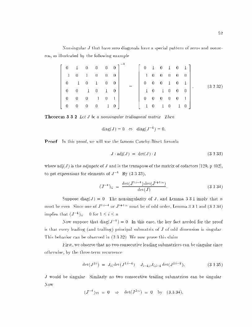
52
Nonsingular J that have zero diagonals have a special pattern of zeros and nonze-
ros, as illustrated by the following example.
26666666666664
0 1 0 0 0 0
�1 0 1 0 0 0
0 �1 0 1 0 0
0 0 �1 0 1 0
0 0 0 �1 0 1
0 0 0 0 �1 0
37777777777775
�1
=
26666666666664
0 1 0 1 0 1
�1 0 0 0 0 0
0 0 0 1 0 1
�1 0 �1 0 0 0
0 0 0 0 0 1
�1 0 �1 0 �1 0
37777777777775: (3.3.32)
Theorem 3.3.2 Let J be a nonsingular tridiagonal matrix. Then
diag(J) = 0 , diag(J�1) = 0:
Proof. In this proof, we will use the famous Cauchy-Binet formula
J � adj(J) = det(J) � I (3.3.33)
where adj(J) is the adjugate of J and is the transpose of the matrix of cofactors [129, p.402],
to get expressions for elements of J�1. By (3.3.33),
(J�1)ii =det(J1:i�1) det(J i+1:n)
det(J): (3.3.34)
Suppose diag(J) = 0. The nonsingularity of J , and Lemma 3.3.1 imply that n
must be even. Since one of J1:i�1 or J i+1:n must be of odd order, Lemma 3.3.1 and (3.3.34)
implies that (J�1)ii = 0 for 1 � i � n.
Now suppose that diag(J�1) = 0. In this case, the key fact needed for the proof
is that every leading (and trailing) principal submatrix of J of odd dimension is singular.
This behavior can be observed in (3.3.32). We now prove this claim.
First, we observe that no two consecutive leading submatrices can be singular since
otherwise, by the three-term recurrence
det(J1:i) = Jii det(J1:i�1)� Ji�1;iJi;i�1 det(J
1:i�2); (3.3.35)
J would be singular. Similarly no two consecutive trailing submatrices can be singular.
Now
(J�1)11 = 0 ) det(J2:n) = 0 by (3:3:34);
53
and hence, det(J3:n) 6= 0. Consequently,
(J�1)22 = 0 ) det(J1:1) = 0; again by (3:3:34):
Similarly by setting i = 3; 4 and so on in (3.3.34), we can conclude that the principal
submatrices J4:n; J1:3; J6:n; J1:5; : : : must be singular. In particular, all leading principal
submatrices of odd dimension are singular. Now, if n is odd then n � 2 is also odd and by
the above reasoning, J1:n�2 is singular. However, by setting i = n in (3.3.34), we see that
det(J1:n�1) = 0;
but no two consecutive principal submatrices of a nonsingular J can be singular. Hence n
cannot be odd, and must be even.
When i is odd, the submatrices J1:i and J1:i�2 are singular and by (3.3.35), we
get
0 = det(J1:i) = Jii det(J1:i�1);
and Jii must be 0 since det(J1:i�1) 6= 0 in this case. Similarly, since n is even and by
considering the trailing recurrence
det(J i:n) = Ji;i det(Ji+1:n)� Ji;i+1Ji+1;i det(J
i+2:n);
we can conclude that Jii = 0 for even i. tuThe pattern of zeros and nonzeros in J�1 that is used to prove the above result
may also be deduced by using the following lemma which states that the upper (lower)
triangular part of J�1 is a rank-one matrix. This result has appeared in [4, 14, 83, 78, 42].
Lemma 3.3.2 Let J be a nonsingular unreduced tridiagonal matrix of order n. Then there
exist vectors x, y, p and q such that
(J�1)ik =
8<: xiyk ; i � k;
piqk ; i � k:
The following corollary says that the spectrum of tridiagonals that have a zero
diagonal is symmetric.
Corollary 3.3.1 Let J be a tridiagonal matrix such that diag(J) = 0. Then if � is an
eigenvalue of J, so is ��. If v and w are the corresponding normalized eigenvectors, then
jv(i)j = jw(i)j for 1 � i � n.
54
Proof. Lemma 3.3.1 implies that eigenvalues occur in � pairs. The corresponding eigen-
vector entries are equal in magnitude by (3.0.8) since �0(�) = ��0(��). tuWe have shown that for all j kj to be 1, all eigenvalues of J = ~J � �I must
occur in � pairs. Thus � is equidistant to the two closest eigenvalues. Note that this
result is consistent with Theorem 3.2.1. We will be careful to avoid this situation in our
application. As we stated in the previous section, we will use Algorithm 3.2.1 to compute
an eigenvector only when the corresponding eigenvalue is \su�ciently isolated" (we make
the meaning of \isolated" more precise in the upcoming chapters). Then, as Theorem 3.2.1
shows, at least one k must be small if � is close to the eigenvalue. Breakdown in the
triangular factorization does not hinder �nding such a k. The corresponding eigenvector
is approximated well by Algorithm 3.3.1 given earlier in this section.
We now show how the ideas developed in this chapter enable us to correctly handle
the matrix T of (3.0.4).
Example 3.3.1 [Minimum j kj leads to a good eigenvector approximation.] Con-
sider T as in (3.0.4) of Example 3.0.1, and the eigenvalue approximation � = 1 so that the
error in the eigenvalue is "+O("2).
(T � I)�1 =
26664
4=(�4 + 3") 0 �p"=(�4 + 3")
0 0 1=p"
�p"=(�4 + 3") 1=p" (�4 + 10"� 5"2)="(�4 + 3")
37775
and since �1k
= (T�1)kk ,
1 � �1; j 2j =1 and 3 � ":
Since j 3j is the minimum, our theory predicts that z = (T � I)�1e3 is a good eigenvector
approximation. Indeed,
z
kzk =
26664"3=2=4 +O("5=2)p"+ O("3=2)
1� "=2 +O("2)
37775 :
and from (3.0.5) we see that each entry of the above vector agrees with the corresponding
eigenvector entry in all its �gures, i.e., the relative error in each entry is O("). tu
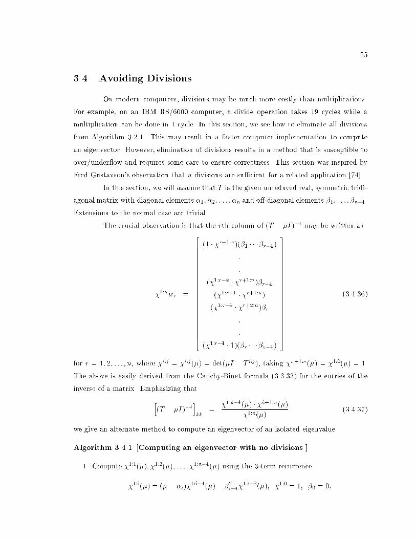
55
3.4 Avoiding Divisions
On modern computers, divisions may be much more costly than multiplications.
For example, on an IBM RS/6000 computer, a divide operation takes 19 cycles while a
multiplication can be done in 1 cycle. In this section, we see how to eliminate all divisions
from Algorithm 3.2.1. This may result in a faster computer implementation to compute
an eigenvector. However, elimination of divisions results in a method that is susceptible to
over/under ow and requires some care to ensure correctness. This section was inspired by
Fred Gustavson's observation that n divisions are su�cient for a related application [74].
In this section, we will assume that T is the given unreduced real, symmetric tridi-
agonal matrix with diagonal elements �1; �2; : : : ; �n and o�-diagonal elements �1; : : : ; �n�1.
Extensions to the normal case are trivial.
The crucial observation is that the rth column of (T � �I)�1 may be written as
�1:nwr =
266666666666666666666664
(1 � �r+1:n)(�1 � � ��r�1):
:
(�1:r�2 � �r+1:n)�r�1(�1:r�1 � �r+1:n)(�1:r�1 � �r+2:n)�r
:
:
(�1:r�1 � 1)(�r � � ��n�1)
377777777777777777777775
(3.4.36)
for r = 1; 2; : : : ; n, where �i:j = �i:j(�) = det(�I � T i:j), taking �n+1:n(�) = �1:0(�) = 1.
The above is easily derived from the Cauchy-Binet formula (3.3.33) for the entries of the
inverse of a matrix. Emphasizing that
h(T � �I)�1
ikk
=�1:k�1(�) � �k+1:n(�)
�1:n(�)(3.4.37)
we give an alternate method to compute an eigenvector of an isolated eigenvalue.
Algorithm 3.4.1 [Computing an eigenvector with no divisions.]
1. Compute �1:1(�); �1:2(�); : : : ; �1:n�1(�) using the 3-term recurrence
�1:i(�) = (�� �i)�1:i�1(�)� �2i�1�
1:i�2(�); �1:0 = 1; �0 = 0:
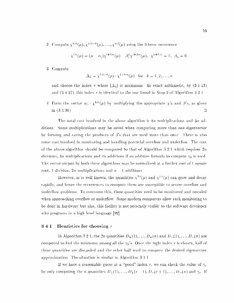
56
2. Compute �n:n(�); �n:n�1(�); : : : ; �n:2(�) using the 3-term recurrence
�i:n(�) = (�� �i)�i+1:n(�)� �2
i�i+2:n(�); �n+1:n = 1; �n = 0:
3. Compute
�k = �1:k�1(�) � �k+1:n(�) for k = 1; 2; : : : ; n
and choose the index r where j�kj is maximum. In exact arithmetic, by (3.1.13)
and (3.4.37), this index r is identical to the one found in Step 2 of Algorithm 3.2.1.
4. Form the vector wr � �1:n(�) by multiplying the appropriate �'s and �'s, as given
in (3.4.36). tu
The total cost involved in the above algorithm is 8n multiplications and 3n ad-
ditions. Some multiplications may be saved when computing more than one eigenvector
by forming and saving the products of �'s that are used more than once. There is also
some cost involved in monitoring and handling potential over ow and under ow. The cost
of the above algorithm should be compared to that of Algorithm 3.2.1 which requires 2n
divisions, 3n multiplications and 4n additions if an additive formula to compute k is used.
The vector output by both these algorithms may be normalized at a further cost of 1 square
root, 1 division, 2n multiplications and n� 1 additions.
However, as is well known, the quantities �1:i(�) and �i:n(�) can grow and decay
rapidly, and hence the recurrences to compute them are susceptible to severe over ow and
under ow problems. To overcome this, these quantities need to be monitored and rescaled
when approaching over ow or under ow. Some modern computers allow such monitoring to
be done in hardware but alas, this facility is not presently visible to the software developer
who programs in a high level language [92].
3.4.1 Heuristics for choosing r
In Algorithm 3.2.1, the 2n quantities D+(1); : : : ; D+(n) and D�(1); : : : ; D�(n) are
computed to �nd the minimum among all the k's. Once the right index r is chosen, half of
these quantities are discarded and the other half used to compute the desired eigenvector
approximation. The situation is similar in Algorithm 3.4.1.
If we have a reasonable guess at a \good" index r, we can check the value of r
by only computing the n quantities D+(1); : : : ; D+(r� 1); D�(r+ 1); : : : ; D�(n) and r. If
57
r is small enough we can accept r, otherwise we can compute all the 's and choose the
minimum as before. In case the guess is accurate, we can save approximately half the work
in the computation of the eigenvector. We now examine the proof of the Gerschgorin Disk
Theorem that suggests a heuristic choice of r.
Theorem 3.4.1 [Gerschgorin Disk Theorem]. Let B be a matrix of order n with an
eigenvalue �. Then � lies in one of the Gerschgorin disks, i.e., 9r such that
j��Brr j �Xk 6=rjBrk j
Proof. Let v be the eigenvector corresponding to �, and let jv(r)j = kvk1. Consider therth equation of Bv = �v,
�v(r) = Brrv(r) +Xk 6=r
Brkv(k)
) j��Brrj �Xk 6=rjBrkjjv(k)=v(r)j
from which the result follows. tuThus if the kth entry of v is the largest, then � must lie in the kth Gerschgorin
disk. Consequently, if � lies in just one Gerschgorin disk then the corresponding entry of v
must be the largest. However � may lie in many Gerschgorin disks and there is no guarantee
that the corresponding entries of v are large. But we may use the following heuristic
Pick r such that � lies in the rth Gerschgorin disk with minimum radiusP
k 6=r jBrkj.
Such a heuristic is inexpensive to compute and can lead to considerable savings
on large matrices, especially ones that are even mildly graded. Such matrices seem to arise
in many real life applications. Note that the above heuristic gives the correct choice of r in
the example tridiagonals of (3.0.4) and (3.0.6).
We do not make any claim about the optimality of the above heuristic, and it may
be possible to obtain better ones. The purpose of this section was to furnish the idea of
heuristically picking r and checking it in order to potentially save half the computations.
3.5 Twisted Q Factorizations | A Digression�
In this section, we introduce twisted QR-type factorizations. The reader who is
pressed for time and is primarily interested in seeing how to adapt inverse iteration to
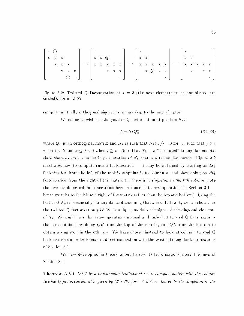
58
266666664
x x
x x x
x x x
x x x
x x
377777775�!
266666664
x
x x x
x x x x x
x x x
x
377777775�!
266666664
x
x x
x x x x x
x x x x
x
377777775�!
266666664
x
x x
x x x x x
x x x
x
377777775
Figure 3.2: Twisted Q Factorization at k = 3 (the next elements to be annihilated are
circled): forming Nk.
compute mutually orthogonal eigenvectors may skip to the next chapter.
We de�ne a twisted orthogonal or Q factorization at position k as
J = NkQ�k (3.5.38)
where Qk is an orthogonal matrix and Nk is such that Nk(i; j) = 0 for i,j such that j > i
when i < k and k � j < i when i � k. Note that Nk is a \permuted" triangular matrix,
since there exists a symmetric permutation of Nk that is a triangular matrix. Figure 3.2
illustrates how to compute such a factorization | it may be obtained by starting an LQ
factorization from the left of the matrix stopping it at column k, and then doing an RQ
factorization from the right of the matrix till there is a singleton in the kth column (note
that we are doing column operations here in contrast to row operations in Section 3.1 |
hence we refer to the left and right of the matrix rather than the top and bottom). Using the
fact thatNk is \essentially" triangular and assuming that J is of full rank, we can show that
the twisted Q factorization (3.5.38) is unique, modulo the signs of the diagonal elements
of Nk. We could have done row operations instead and looked at twisted Q factorizations
that are obtained by doing QR from the top of the matrix, and QL from the bottom to
obtain a singleton in the kth row. We have chosen instead to look at column twisted Q
factorizations in order to make a direct connection with the twisted triangular factorizations
of Section 3.1.
We now develop some theory about twisted Q factorizations along the lines of
Section 3.1.
Theorem 3.5.1 Let J be a nonsingular tridiagonal n� n complex matrix with the column
twisted Q factorization at k given by (3.5.38) for 1 � k � n. Let �k be the singleton in the
59
kth column of Nk, i.e., �k = Nk(k; k). Then
1
j�kj2= e�k(JJ
�)�1ek: (3.5.39)
Proof.
JJ� = NkQ�kQkN
�k
) e�k(JJ�)�1ek = e�kN
��k N�1
k ek :
Since Nkek = �kek , the result (3.5.39) follows. tuWe could endeavor to get expressions for �k, as we did for k in (3.1.12), in terms
of the left and right factorizations. In particular, we can attempt to express �k in terms of
the Schur parameters fcos �+k ; k = 1; : : : ; n� 1g, fcos ��k ; k = 1; : : : ; n � 1g that determinethe orthogonal matrices in the L+Q+ and R�Q� factorizations, and the diagonal elements
of L+ and R�. However, we choose not to do so since the expressions are not stated simply
with our present notation, and do not add to our exposition.
The following results parallel those of Sections 3.1 and 3.2 as do the corresponding
proofs.
Corollary 3.5.1 Let J be a nonsingular tridiagonal matrix. With the notation of Theo-
rem 3.5.1,nXi=1
j�ij�2 = Trace((JJ�)�1) =nXi=1
��2i ;
where �1; �2; : : : ; �n are the singular values of J.
Theorem 3.5.2 Let J = ~J��I be a tridiagonal matrix with the twisted factorization (3.5.38)
for a �xed value of k. Then
( ~J � �I)qk = �kek ;
where qk is the kth column of Qk.
Proof. Since Nkek = �kek and ~J � �I = NkQ�k,
( ~J � �I)Qk = Nk ) ( ~J � �I)qk = �kek :
tuThus the vector qk is just a normalized version of z(k) de�ned in (3.2.25) in The-
orem 3.2.2. The following theorems con�rm that the corresponding residual norms are
equal.
60
Theorem 3.5.3 Let J = ~J � �I be a nonsingular tridiagonal matrix and let �k, k and
z(k) be as de�ned in (3.5.39), (3.1.13) and (3.2.25) respectively. Then
j kjkz(k)k = j�kj (3.5.40)
Proof. Since ( ~J � �I)z(k) = kek,
kz(k)k2j kj2
= e�k( ~J � �I)��( ~J � �I)�1ek
=1
j�kj2:
The last equality is just (3.5.39). tuThus when J is normal, the bound (3.2.28) for j kj=kz(k)k applies to j�kj. The
connection between qk and z(k) suggests the following alternative to Algorithm 3.2.1 that
is guaranteed to �nd a small �k for a nearly singular ~J ��I , even when the eigenvalue near
� is not isolated.
Algorithm 3.5.1 [Computing an eigenvector of any eigenvalue.]
1. Compute the diagonal elements �k for all n twisted Q factorizations of ~J .
2. Choose the index r where j�kj is minimum.
3. Form the vector qr, where qr is as in Theorem 3.5.2.
tu
The above results may appear somewhat surprising but the reader is reminded of
the intimate connection between the LR algorithm, the QR algorithm and inverse itera-
tion [110]. For a non-normal matrix also, as the following theorem implies, there is at least
one �k that indicates its nearness to singularity.
Theorem 3.5.4 Let B be a nonsingular matrix of order n. Let �min = �n be the smallest
singular value of B and umin be the corresponding left singular vector. If
1
j�k j2= e�k(BB
�)�1ek for k = 1; 2; : : : ; n
then
j�kj =�min
jumin(k)jh1 +
�jumin(k)j�2 � 1
�A2
i�1=2;
� �min
jumin(k)j� p
n �min for at least one k
61
where A2 is a weighted arithmetic mean of
���min�i
�2; i < n
�, 0 < A2 < (�min=�n�1)
2.
Proof. The proof is similar to that of Theorem 3.2.3 using the following eigendecomposition
of BB�,
BB� = U�2U�:
tuIn Section 3.1, we showed that k = 0 when J is singular and admits the triangular
decompositions (3.1.11) (see Corollary 3.1.4 and the comments immediately following it).
Similarly, it can be shown that if J is an unreduced tridiagonal that is singular, then �k = 0
in the factorization of (3.5.38) for any k.
3.5.1 \Perfect" Shifts are perfect
In this section, we give an application of twisted Q factorizations. If � is an
eigenvalue of the unreduced tridiagonal ~J , then the last diagonal element of R, Rnn, in the
factorization
~J � �I = QR; Q�Q = I; R upper triangular
must be zero in exact arithmetic. The QR iteration on ~J with shift � yields ~J1 :
~J � �I = QR; RQ+ �I = ~J1:
When � = �, the (n� 1; n) entry of the tridiagonal ~J1 is zero and hence � may be de ated
from ~J1 by simply removing the last row and column.
It may be expected that if � is close to �, then Rnn would be small and de ation
would again occur in one iteration. Based on this expectation, Parlett proposed the following
strategy to compute all the eigenvalues and eigenvectors of a real, symmetric tridiagonal
matrix T [110, p.173].
1. Compute eigenvalues by a fast algorithm such as the PWK algorithm, which is a QR
algorithm free of square roots.
2. Run the QR algorithm using the computed eigenvalues as shifts, accumulating the
rotations to form the eigenvector matrix.
The expectation was that de ation would occur in one step, thus saving approx-
imately 50% of the dominant O(n3) computation in the QR algorithm, which typically
requires an average of 2-3 iterations per eigenvalue.
62
However,
T � �I = QR
) eTn (T � �I)�2en =1
jRnnj2
)nXi=1
jvi(n)j2(�i � �)2
=1
jRnnj2
showing that if the bottom entry of the desired eigenvector is tiny, then Rnn is not small.
As a result, immediate de ation is not always seen in the perfect-shift QR algorithm, and
it was found not to perform any better than the standard QR algorithm with Wilkinson's
shift [69]. The situation is similar to that with D+(n) discused in Section 3.1. And it is
natural for us, as in Section 3.1, to turn to twisted factorizations to detect singularity of
T � �I . Let
T � �I = QkNk (3.5.41)
be a twisted Q factorization of T � �I . This is essentially identical to the column twisted
L factorization of J in (3.5.38) since T is symmetric. In the above factorization the kth
row of Nk is a singleton with a non-zero on the diagonal. By the theory developed in the
previous section, in particular Theorem 3.5.4, there must be a k such that Nk(k; k) is small
if � is a good approximation to an eigenvalue of T .
With this choice of k, we can form the matrix
A1 = NkQk + �I (3.5.42)
following the standard QR algorithm. Since �k is small all the o�-diagonal entries of the
kth row of A1 must be small. Since A1 = Q�kTQk is symmetric the o�-diagonal entries in
the kth column are also tiny. An eigenvalue close to � may be de ated by crossing out the
entire kth row and column of A1. Thus de ation occurs in exactly one step when perfect
shifts are used. For a more detailed treatment, the reader should wait for [41].
Each matrix in the sequence obtained in the standard QR algorithm is tridiago-
nal. Does (3.5.42) preserve tridiagonal form? The reduction uniqueness theorem in [110,
Section 7-2] states that a tridiagonal formed by an orthogonal similarity transformation,
T = Q�AQ, is determined by A and the �rst or last column of Q. It follows that A1 cannot
be tridiagonal in general since, except when k = 1 or n, the �rst and last columns of Qk
in (3.5.41) are independent. However, it can be shown that the matrix obtained by delet-
ing the kth row and column of A1 is tridiagonal with an additional bulge at new position
63
(k + 1; k) after de ation. This bulge can then be \chased" out of the top or bottom of the
matrix, whichever is nearer. This yields a tridiagonal matrix to which the next perfect shift
may now be applied.
To form the eigenvector matrix the n� 1 rotations that form Qk must be accumu-
lated as must be the rotations used to chase the bulge out of the end of the de ated matrix.
Thus in the worst case 1:5 iterations are needed per eigenvalue to compute the eigenvectors.
Assuming 1-1.5 iterations per eigenvalue, all the eigenvectors may be obtained at a cost of
3n3-4:5n3 operations. This is about twice as fast as current QR algorithms, assuming that
n is large enough to disregard the extra computation involved in the initial computation of
the eigenvalues and in �nding k at each step. Heuristics for guessing k may also be used as
discussed in Section 3.4.1.
Standard QR algorithms use an implicit version to achieve greater accuracy. It
remains to be seen if similar techniques may be used in the algorithm outlined above. It
should also be possible to �nd k by using a procedure free from square roots as in the PWK
algorithm. But as we mentioned earlier, this section is a digression from the main theme of
this thesis and we plan to explore these questions elsewhere [41].
The reader may wonder about our inconsistency in �nding the eigenvalues by a
standard QR algorithm but using twisted factorizations in �nding the eigenvectors. Is it
not possible to use twisted factorizations to �nd the eigenvalues also? We believe that
the latter might indeed be the right approach not only in speeding up the algorithm but
also to get higher accuracy since the standard QR algorithm may violently rearrange the
matrix thereby destroying accuracy [32]. However, this is not straightforward due to the
complication that A1 in (3.5.42) is not tridiagonal. When de ation does not occur, chasing
the bulges in A1 o� the top or bottom of the matrix will give the standard QR or QL
algorithm respectively (by the reduction uniqueness theorem in [110, Section 7-2]). Thus
in order to develop a \twisted algorithm", we must give up the tridiagonal nature of the
intermediate matrices. The number of bulges increase by 2 at each step, and it is for
future research to determine if it is computationally feasible to handle this increase. We
also believe that such a twisted algorithm may lead to better shifts than the Francis or
Wilkinson shifts.
64
3.6 Rank Revealing Factorizations�
In earlier sections of this study, we exhibited twisted triangular and twisted or-
thogonal (or Q) factorizations for tridiagonals. In our applications, we were successfully
able to reveal the singularity of the tridiagonal by one of the n possible twisted factors.
In this section, we show that such factorizations can also be done for denser matri-
ces and may be used to reveal the rank of the matrix. We convey our ideas through pictures
and make no pretence to being complete in this section.
Formally, we de�ne a row twisted triangular factorization of a matrix B at posi-
tion k as the decomposition
B = NkDk~Nk (3.6.43)
where Dk is diagonal, while Nk and ~Nk are such that (Nk)ij = 0 for i,j such that j > i when
i < k and k � j < i otherwise, and ~N�k has the same requirement on its zeros. We take
both Nk and ~Nk to have 1's on their diagonals. Note that Nk and ~Nk are simultaneously
permuted triangular matrices, i.e., 9 a permutation Pk such that PTk NkPk is lower triangular
and PTk~NkPk is upper triangular. (3.6.43) may be written as
PTk BPk = (PT
k NkPk)(PTk DkPk)(P
Tk~NkPk)
and this is just the LDU decomposition of PTk BPk . This implies the uniqueness of the
factorization in (3.6.43).
Figures 3.3 and 3.5 suggest a way to compute the twisted LU decomposition for
Hessenberg and dense matrices respectively. Note that when B is normal, Theorem 3.2.1
is applicable with k = Dk(k; k). Thus when B is nearly singular with an isolated small
eigenvalue, Theorem 3.2.1 implies the existence of a small bottom pivot in all possible
LU -factorizations of B that can be obtained by symmetric permutations of the rows and
columns of B. A generalization of such a result was proved by Tony Chan in 1984 [19] (he
considered non-normal B as well, and arbitrary row and column permutations of B). We
brie y compare our results with Chan's results of [19] at the end of this section.
We now formally de�ne a row twisted Q decomposition of B at position k as
B = QkNk (3.6.44)
where Qk is orthogonal andNk is a permuted triangular matrix as made precise earlier in this
section. Figures 3.4 and 3.5 suggest computational procedures to �nd such a factorization
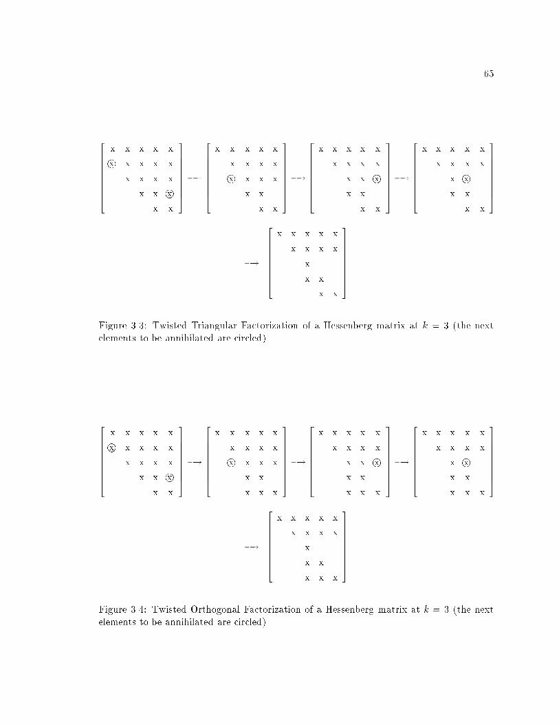
65
266666664
x x x x x
x x x x x
x x x x
x x x
x x
377777775�!
266666664
x x x x x
x x x x
x x x x
x x
x x
377777775�!
266666664
x x x x x
x x x x
x x x
x x
x x
377777775�!
266666664
x x x x x
x x x x
x x
x x
x x
377777775
�!
266666664
x x x x x
x x x x
x
x x
x x
377777775
Figure 3.3: Twisted Triangular Factorization of a Hessenberg matrix at k = 3 (the next
elements to be annihilated are circled)
266666664
x x x x x
x x x x x
x x x x
x x x
x x
377777775�!
266666664
x x x x x
x x x x
x x x x
x x
x x x
377777775�!
266666664
x x x x x
x x x x
x x x
x x
x x x
377777775�!
266666664
x x x x x
x x x x
x x
x x
x x x
377777775
�!
266666664
x x x x x
x x x x
x
x x
x x x
377777775
Figure 3.4: Twisted Orthogonal Factorization of a Hessenberg matrix at k = 3 (the next
elements to be annihilated are circled)
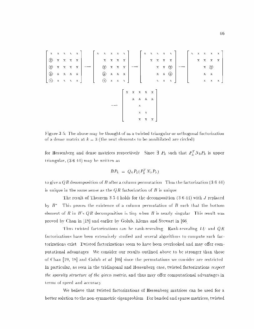
66
266666664
x x x x x
x x x x x
x x x x x
x x x x x
x x x x x
377777775�!
266666664
x x x x x
x x x x
x x x x
x x x x
x x x x
377777775�!
266666664
x x x x x
x x x x
x x x
x x x
x x x
377777775�!
266666664
x x x x x
x x x x
x x
x x
x x x
377777775
�!
266666664
x x x x x
x x x x
x
x x
x x x
377777775
Figure 3.5: The above may be thought of as a twisted triangular or orthogonal factorization
of a dense matrix at k = 3 (the next elements to be annihilated are circled)
for Hessenberg and dense matrices respectively. Since 9 Pk such that PTk NkPk is upper
triangular, (3.6.44) may be written as
BPk = QkPk(PTk NkPk)
to give aQR decomposition ofB after a column permutation. Thus the factorization (3.6.44)
is unique in the same sense as the QR factorization of B is unique.
The result of Theorem 3.5.4 holds for the decomposition (3.6.44) with J replaced
by B�. This proves the existence of a column permutation of B such that the bottom
element of R in B's QR decomposition is tiny when B is nearly singular. This result was
proved by Chan in [18] and earlier by Golub, Klema and Stewart in [66].
Thus twisted factorizations can be rank-revealing. Rank-revealing LU and QR
factorizations have been extensively studied and several algorithms to compute such fac-
torizations exist. Twisted factorizations seem to have been overlooked and may o�er com-
putational advantages. We consider our results outlined above to be stronger than those
of Chan [19, 18] and Golub et al. [66] since the permutations we consider are restricted.
In particular, as seen in the tridiagonal and Hessenberg case, twisted factorizations respect
the sparsity structure of the given matrix, and thus may o�er computational advantages in
terms of speed and accuracy.
We believe that twisted factorizations of Hessenberg matrices can be used for a
better solution to the non-symmetric eigenproblem. For banded and sparse matrices, twisted
67
factorizations may o�er considerable savings in computing rank-revealing factorizations. We
intend to conduct further research in these two areas. The innovative reader may be able
to think of other applications.
68
Chapter 4
Computing orthogonal
eigenvectors when relative gaps
are large
In the last chapter, we showed how to compute the eigenvector corresponding to
an isolated eigenvalue of a normal, unreduced tridiagonal matrix. In particular, we showed
how to choose a right hand side for inverse iteration that has a guaranteed large component
in the direction of the desired eigenvector. Even though this is both a theoretical and
practical advance, it does not solve the most pressing problem with inverse iteration |
that of computing approximate eigenvectors that are numerically orthogonal.
When eigenvalues are well separated, vectors that give a small residual norm,
as in (1.1.1), are numerically orthogonal. In such a case, the methods of Chapter 3 are
su�cient. However this is not the case with close eigenvalues and current implementations
of inverse iteration resort to explicit orthogonalization. As mentioned in Chapter 1 and
Section 2.8.1 this can take an inordinately large amount of computation, and even then,
the computed vectors may not be numerically orthogonal.
The rest of this thesis is devoted to the computation of \good eigenvectors" that are
automatically numerically orthogonal thus avoiding the need for explicit orthogonalization.
In this chapter, we show that an alternate representation of a tridiagonal is the key to better
approximations. Coupled with the theory developed in Chapter 3 this allows us to compute
orthogonal eigenvectors when the corresponding eigenvalues have large relative gaps, even
though the eigenvalues may be very close together in an absolute sense. More precisely,
69
1. In Section 4.1, we extol the virtues of high accuracy. Tridiagonals do not always
\allow" such high accuracy computations and in Section 4.2, we advocate representing
the tridiagonal as a product of bidiagonal matrices.
2. In Section 4.3, we recap earlier work on relative perturbation theory as applied to
bidiagonal matrices.
3. In Section 4.4.1, we give qd-like recurrences that allow us to exploit the properties of
bidiagonals in order to compute highly accurate approximations to eigenvectors. In
Section 4.4.2, we do a roundo� error analysis of their computer implementations while
in Section 4.4.3 we give an algorithm to compute eigenvectors based on these qd-like
recurrences.
4. In Section 4.5 we prove that the dot products between the eigenvectors computed by
the algorithm given in Section 4.4.3 are inversely proportional to the relative gaps
between eigenvalues. As a consequence, the computed eigenvectors are numerically
orthogonal if the corresponding eigenvalues are relatively far apart. These results
are new and are a major advance towards our goal of obtaining guaranteed numerical
orthogonality in O(n2) time.
5. In Section 4.6, we present numerical results that support the above claims.
We consider the case of eigenvalues that have small relative gaps in the next two chapters.
4.1 Bene�ts of High Accuracy
Consider the matrix T0 in (2.8.16) of Section 2.8.1,
T0 =
26664
1p" 0
p" 7"=4 "=4
0 "=4 3"=4
37775
where " is the machine precision. T0 has two small eigenvalues �1 = "=2 + O("2) and
�2 = " + O("2), while �3 � 1. Suppose that �1 and �2 are approximations to �1 and �2,
and inverse iteration as in (2.7.4) is used to �nd the corresponding eigenvectors. In exact
arithmetic, taking b1 =P
i �ivi and b2 =P
i �ivi, kb1k = kb2k = 1, we get
y1 = (T0 � �1I)�1b1 =
�1
�1 � �1
v1 +
�2
�1
�1 � �1
�2 � �1v2 +
�3
�1
�1 � �1
�3 � �1v3
!; (4.1.1)
70
y2 = (T0 � �2I)�1b2 =
�2
�2 � �2
�1
�2
�2 � �2
�1 � �2v1 + v2 +
�3
�2
�2 � �2
�3 � �2v3
!: (4.1.2)
We assume that �1, �2, �1 and �2 are O(1). Earlier we showed that y1 and y2 are
nearly parallel if �1 � �2, and in such a case, EISPACK and LAPACK implementations fail
to deliver orthogonal vectors despite explicit orthogonalization. See Section 2.8.1 and Case
Study A for more details. It is clearly desirable that �1 and �2 be more accurate so that
their di�erence is discernible. Given limited precision to represent numbers in a computer,
how accurate can �1 and �2 be? We say that �i agrees with �i to d digits if
j�i � �ijj�ij
= 10�d:
The IEEE double precision format allows for 53 bits of precision, thus " = 2�52 �2:2 � 10�16 and d can take a maximum value of about 16. Suppose �1 and �2 agree with �1
and �2 respectively to d digits, where d � 1. Since �1 and �2 do not agree in any digit,
j�i � �ijj�j � �ij
= O(10�d) where i = 1; 2; j 6= i
and by (4.1.1) and (4.1.2),
jyT1 y2jky1k � ky2k
= O
j�1 � �1jj�2 � �1j
+j�2 � �2jj�1 � �2j
!= O(10�d):
Thus the more accurate �1 and �2 are, the more orthogonal are y1 and y2. In fact when
d = 16, i.e., when �1 and �2 have full relative accuracy, y1 and y2 are numerically orthogonal
and no further orthogonalization is needed.
Of course, the above is true only in exact arithmetic. We now see why the standard
representation of a tridiagonal matrix does not allow computation of eigenvalues to such
high accuracy.
4.2 Tridiagonals Are Inadequate
A real, symmetric tridiagonal matrix T is traditionally represented by its 2n � 1
diagonal and o�-diagonal elements. In this section, we show that for our computational
purposes it is better to represent T by its bidiagonal factors.
To account for the roundo� errors that occur in a computer implementation, it is
common practice to show that the computed eigenvalues and eigenvectors are exact for a
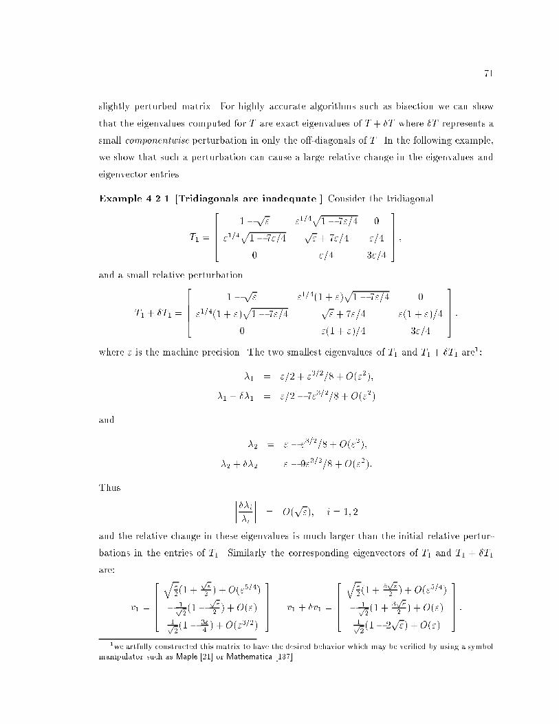
71
slightly perturbed matrix. For highly accurate algorithms such as bisection we can show
that the eigenvalues computed for T are exact eigenvalues of T + �T where �T represents a
small componentwise perturbation in only the o�-diagonals of T . In the following example,
we show that such a perturbation can cause a large relative change in the eigenvalues and
eigenvector entries.
Example 4.2.1 [Tridiagonals are inadequate.] Consider the tridiagonal
T1 =
26664
1�p" "1=4p1� 7"=4 0
"1=4p1� 7"=4
p" + 7"=4 "=4
0 "=4 3"=4
37775 ;
and a small relative perturbation
T1 + �T1 =
26664
1�p" "1=4(1 + ")p1� 7"=4 0
"1=4(1 + ")p1� 7"=4
p" + 7"=4 "(1 + ")=4
0 "(1 + ")=4 3"=4
37775 :
where " is the machine precision. The two smallest eigenvalues of T1 and T1 + �T1 are1:
�1 = "=2 + "3=2=8 +O("2);
�1 + ��1 = "=2� 7"3=2=8 +O("2)
and
�2 = " � "3=2=8 +O("2);
�2 + ��2 = " � 9"3=2=8 +O("2):
Thus ������i�i���� = O(
p"); i = 1; 2
and the relative change in these eigenvalues is much larger than the initial relative pertur-
bations in the entries of T1. Similarly the corresponding eigenvectors of T1 and T1 + �T1
are:
v1 =
26664q
"2(1 +
p"2 ) +O("5=4)
� 1p2(1�
p"2) +O(")
1p2(1� 3"
4) +O("3=2)
37775 v1 + �v1 =
26664q
"2(1 +
5p"
2 ) +O("5=4)
� 1p2(1 + 3
p"
2) + O(")
1p2(1� 2
p") +O(")
37775 :
1we artfully constructed this matrix to have the desired behavior which may be veri�ed by using a symbol
manipulator such as Maple [21] or Mathematica [137]
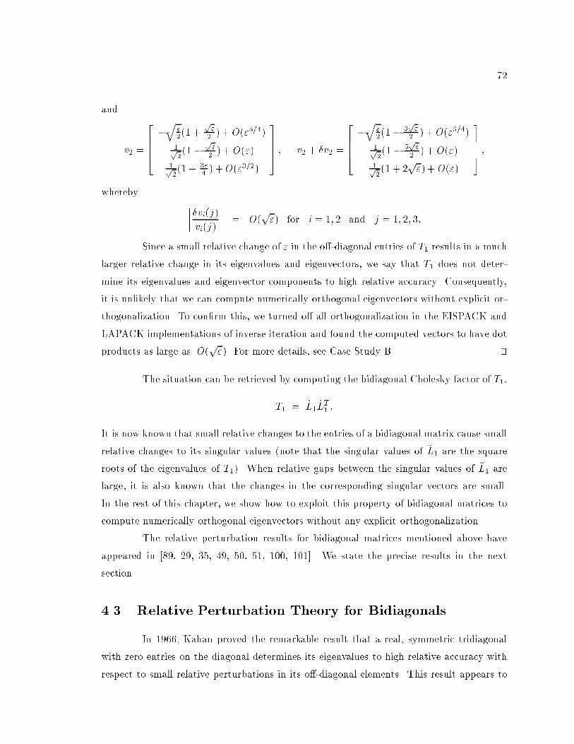
72
and
v2 =
26664�q
"2(1 +
p"2 ) +O("5=4)
1p2(1�
p"2) + O(")
1p2(1 + 3"
4) +O("3=2)
37775 ; v2 + �v2 =
26664�q
"2(1� 3
p"
2 ) + O("5=4)
1p2(1� 5
p"
2) + O(")
1p2(1 + 2
p") + O(")
37775 ;
whereby �����vi(j)vi(j)
���� = O(p") for i = 1; 2 and j = 1; 2; 3:
Since a small relative change of " in the o�-diagonal entries of T1 results in a much
larger relative change in its eigenvalues and eigenvectors, we say that T1 does not deter-
mine its eigenvalues and eigenvector components to high relative accuracy. Consequently,
it is unlikely that we can compute numerically orthogonal eigenvectors without explicit or-
thogonalization. To con�rm this, we turned o� all orthogonalization in the EISPACK and
LAPACK implementations of inverse iteration and found the computed vectors to have dot
products as large as O(p"). For more details, see Case Study B. tu
The situation can be retrieved by computing the bidiagonal Cholesky factor of T1,
T1 = ~L1~LT1 :
It is now known that small relative changes to the entries of a bidiagonal matrix cause small
relative changes to its singular values (note that the singular values of ~L1 are the square
roots of the eigenvalues of T1). When relative gaps between the singular values of ~L1 are
large, it is also known that the changes in the corresponding singular vectors are small.
In the rest of this chapter, we show how to exploit this property of bidiagonal matrices to
compute numerically orthogonal eigenvectors without any explicit orthogonalization.
The relative perturbation results for bidiagonal matrices mentioned above have
appeared in [89, 29, 35, 49, 50, 51, 100, 101]. We state the precise results in the next
section.
4.3 Relative Perturbation Theory for Bidiagonals
In 1966, Kahan proved the remarkable result that a real, symmetric tridiagonal
with zero entries on the diagonal determines its eigenvalues to high relative accuracy with
respect to small relative perturbations in its o�-diagonal elements. This result appears to
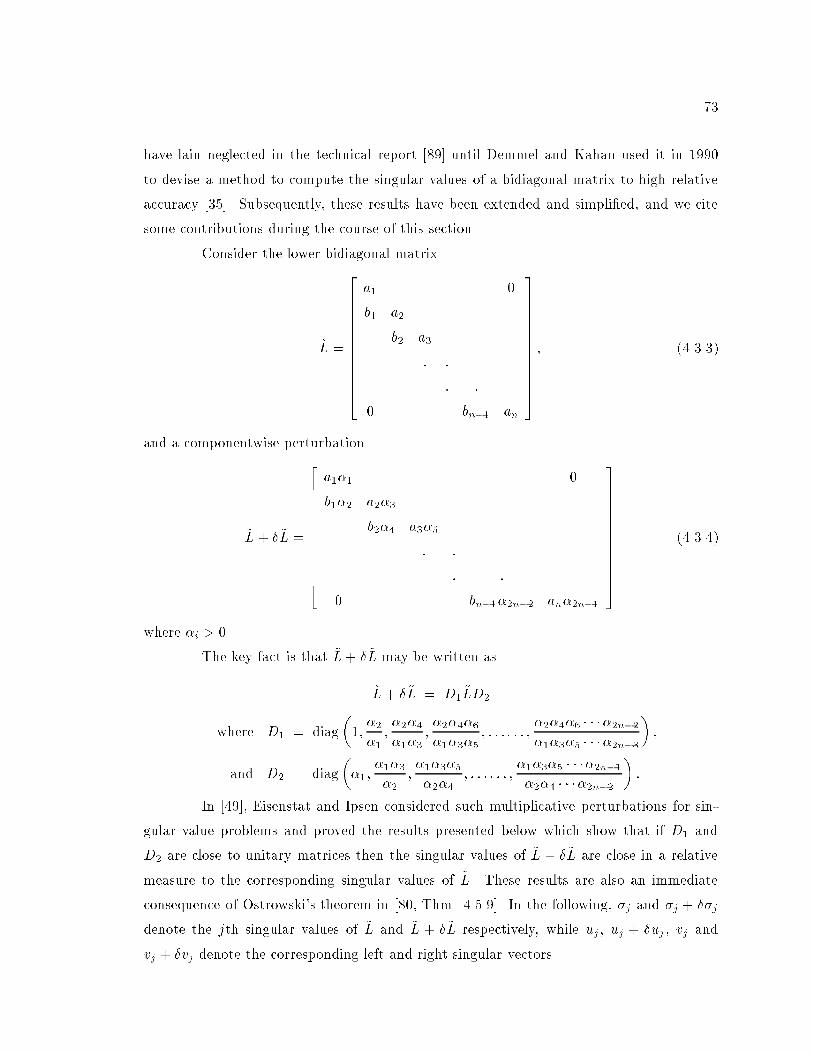
73
have lain neglected in the technical report [89] until Demmel and Kahan used it in 1990
to devise a method to compute the singular values of a bidiagonal matrix to high relative
accuracy [35]. Subsequently, these results have been extended and simpli�ed, and we cite
some contributions during the course of this section.
Consider the lower bidiagonal matrix
~L =
26666666666664
a1 0
b1 a2
b2 a3
: :
: :
0 bn�1 an
37777777777775; (4.3.3)
and a componentwise perturbation
~L+ � ~L =
26666666666664
a1�1 0
b1�2 a2�3
b2�4 a3�5
: :
: :
0 bn�1�2n�2 an�2n�1
37777777777775
(4.3.4)
where �i > 0.
The key fact is that ~L+ � ~L may be written as
~L+ � ~L = D1~LD2
where D1 = diag
�1;�2
�1;�2�4
�1�3;�2�4�6
�1�3�5; : : : : : : ;
�2�4�6 � � ��2n�2�1�3�5 � � ��2n�3
�;
and D2 = diag
��1;
�1�3
�2;�1�3�5
�2�4; : : : : : : ;
�1�3�5 � � ��2n�1�2�4 � � ��2n�2
�:
In [49], Eisenstat and Ipsen considered such multiplicative perturbations for sin-
gular value problems and proved the results presented below which show that if D1 and
D2 are close to unitary matrices then the singular values of ~L + � ~L are close in a relative
measure to the corresponding singular values of ~L. These results are also an immediate
consequence of Ostrowski's theorem in [80, Thm. 4.5.9]. In the following, �j and �j + ��j
denote the jth singular values of ~L and ~L + � ~L respectively, while uj , uj + �uj , vj and
vj + �vj denote the corresponding left and right singular vectors.
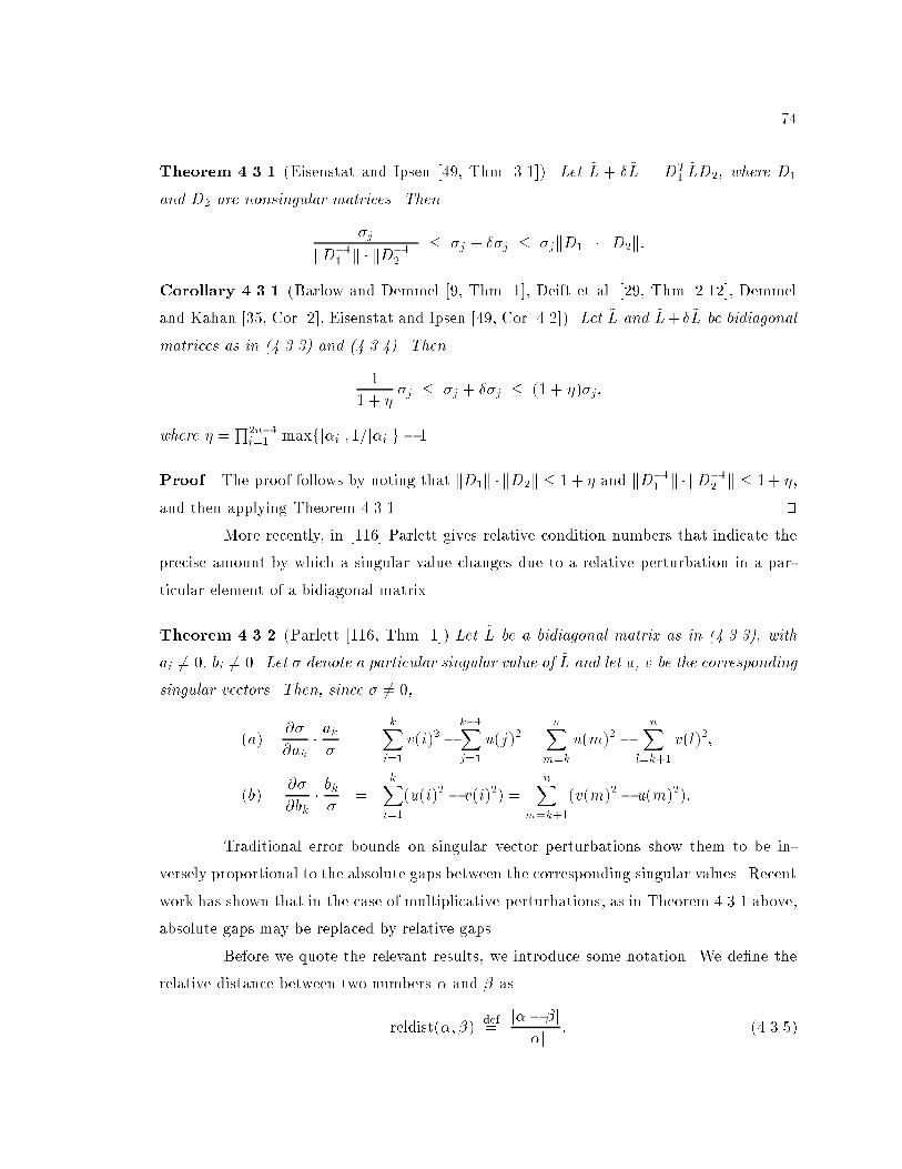
74
Theorem 4.3.1 (Eisenstat and Ipsen [49, Thm. 3.1]). Let ~L + � ~L = DT1~LD2, where D1
and D2 are nonsingular matrices. Then
�j
kD�11 k � kD�1
2 k� �j + ��j � �jkD1k � kD2k:
Corollary 4.3.1 (Barlow and Demmel [9, Thm. 1], Deift et al. [29, Thm. 2.12], Demmel
and Kahan [35, Cor. 2], Eisenstat and Ipsen [49, Cor. 4.2]). Let ~L and ~L+ � ~L be bidiagonal
matrices as in (4.3.3) and (4.3.4). Then
1
1 + ��j � �j + ��j � (1 + �)�j;
where � =Q2n�1
i=1 maxfj�ij; 1=j�ijg � 1.
Proof. The proof follows by noting that kD1k � kD2k � 1+ � and kD�11 k � kD�1
2 k � 1+ �,
and then applying Theorem 4.3.1. tuMore recently, in [116] Parlett gives relative condition numbers that indicate the
precise amount by which a singular value changes due to a relative perturbation in a par-
ticular element of a bidiagonal matrix.
Theorem 4.3.2 (Parlett [116, Thm. 1]) Let ~L be a bidiagonal matrix as in (4.3.3), with
ai 6= 0, bi 6= 0. Let � denote a particular singular value of ~L and let u, v be the corresponding
singular vectors. Then, since � 6= 0,
(a)@�
@ak� ak�
=kXi=1
v(i)2�k�1Xj=1
u(j)2 =nX
m=k
u(m)2 �nX
l=k+1
v(l)2;
(b)@�
@bk� bk�
=kXi=1
(u(i)2 � v(i)2) =nX
m=k+1
(v(m)2� u(m)2):
Traditional error bounds on singular vector perturbations show them to be in-
versely proportional to the absolute gaps between the corresponding singular values. Recent
work has shown that in the case of multiplicative perturbations, as in Theorem 4.3.1 above,
absolute gaps may be replaced by relative gaps.
Before we quote the relevant results, we introduce some notation. We de�ne the
relative distance between two numbers � and � as
reldist(�; �)def=j�� �jj�j : (4.3.5)
75
By the above de�nition, reldist(�; �) 6= reldist(�; �). On the other hand, the measures
reldistp(�; �)def=
j�� �jppj�jp + j�jp : (4.3.6)
are symmetric for 1 � p � 1. Note that
reldist1(�; �)def=
j�� �jmax(j�j; j�j): (4.3.7)
For more discussion and comparison between these measures, see [100]. Relative gaps
between singular values will �gure prominently in our discussion, and we de�ne
relgap(�; f�g) def= min
y2f�greldist(�; y); (4.3.8)
where � is a real number while f�g denotes a set of real numbers. Typically, f�g will denotea subset of the singular values. Similarly, we de�ne the relative gaps for the symmetric
measures to be
relgapp(�; f�g) def= min
y2f�greldistp(�; y):
The following theorem bounds the perturbation angle in terms of the relative gaps.
It is a special case of Li's Theorem 4.7 [101].
Theorem 4.3.3 Let ~L + � ~L = DT1~LD2, where D1 and D2 are nonsingular matrices. If
�i + ��i 6= �j for i 6= j, then
j sin 6 (uj ; uj + �uj)j �qkI �DT
1 k2 + kI �D�11 k+ kI �DT
2 k2 + kI �D�12 k
relgap2(�j ; f�i + ��iji 6= jg) :
Corollary 4.3.2 Let ~L and ~L + � ~L be bidiagonal matrices as in (4.3.3) and (4.3.4). If
�i + ��i 6= �j for i 6= j, then
j sin 6 (uj ; uj + �uj)j ��
relgap2(�j ; f�i + ��iji 6= jg);
where � =Q2n�1
i=1 maxfj�ij; 1=j�ijg � 1.
See also Eisenstat and Ipsen [49, Theorem 3.3 and Cor. 4.5].
The above results can be generalized to singular subspaces of larger dimension.
Before we present the results, we need to introduce additional notation. We partition the
singular value decomposition of the square matrices ~L and ~L+ � ~L as
~L = U�V T = (U1; U2)
0@ �1 0
0 �2
1A0@ V T
1
V T2
1A ;
76
and
~L+ � ~L = (U1 + �U1; U2 + �U2)
0@ �1 + ��1 0
0 �2 + ��2
1A0@ V T
1 + �V T1
V T2 + �V T
2
1A ;
where �1 = diag(�1; : : : ; �k) and �2 = diag(�k+1+ ��k+1; : : : ; �n+ ��n) for 1 � k < n, and
the other arrays are partitioned conformally. In such a case, we measure the angle between
the eigenvector uj and the invariant subspace U1 + �U1, j � k, as
k sin 6 (uj ; U1 + �U1)k = k(UT2 + �UT
2 )ujk:
For more on angles between subspaces, see [67, Section 12.4.3]. The following is an easily
obtained extension of Theorem 4.8 in [101].
Theorem 4.3.4 Let ~L+ � ~L = DT1~LD2, where D1 and D2 are nonsingular matrices. If
maxk<i�n
�i + ��i < min1�l�k
�l;
then for j � k and 1 � p � 1,
k sin 6 (uj ; U1 + �U1)k �max
�qkI �D�1
2 k2 + kI �DT1 k2;
qkI �D�1
1 k2 + kI �DT2 k2
�relgapp(�j ; f�i + ��ijk < i � ng) :
Corollary 4.3.3 Let ~L and ~L+ � ~L be bidiagonal matrices as in (4.3.3) and (4.3.4). If
maxk<i�n
�i + ��i < min1�l�k
�l;
then for j � k and 1 � p � 1,
k sin 6 (uj ; U1 + �U1)k ��
relgapp(�j ; f�i + ��ijk < i � ng) ;
where � =Q2n�1
i=1 maxfj�ij; 1=j�ijg � 1.
See also Eisenstat and Ipsen [50, Theorem 3.1].
4.4 Using Products of Bidiagonals
We now show how to exploit the properties of a bidiagonal matrix that were out-
lined in the previous section. Consider the tridiagonal matrix T1 given in Example 4.2.1. In
77
section 4.2, we gave the inherent limitations of using the 2n�1 diagonal and o�-diagonal el-ements of T1. Since T1 is positive de�nite we can compute its bidiagonal Cholesky factor ~L1.
The singular values, �j , of ~L1 may now be computed to high relative accuracy using either
bisection or the much faster and more elegant dqds algorithm given in [56] (remember that
in exact arithmetic the eigenvalues of T1 are the squares of the singular values of ~L1 and
the eigenvectors of T1 are the left singular vectors of ~L1). Recall that the singular values of
~L1 are such that
�21 = "=2 +O("2); �22 = " +O("2); and �23 = 1 + O("):
As a consequence of the large relative gaps between the singular values, the singular vectors
of ~L1 are \well-determined" with respect to small componentwise perturbations in entries
of ~L1. We can now compute these singular vectors by using a method similar to Algo-
rithm 3.2.1 of Chapter 3. In spite of being computed independently, these vectors will turn
out to be numerically orthogonal!
The errors made in computing the Cholesky factor ~L1 are irrelevant to the orthog-
onality of the computed vectors. Cholesky factorization is known to be backward stable
and it can be shown that the computed ~L1 is the exact Cholesky factor of T1 + �T1 where
k�T1k = O("kT1k). Thus small residual norms with respect to ~L1~L1
Ttranslate to small
residual norms with respect to T1, i.e.,
k(~L1~LT1 � �2j I)vk = O("k~L1
~LT1 k)
) k(T1 � �2j I)vk = O("kT1k):
The dual goals of orthogonality and small residual norms will thus be satis�ed in this case
(see (1.1.1) and (1.1.2)).
The tridiagonal matrix of Example 4.2.1 is positive de�nite. In general, the matrix
T whose eigendecomposition is to be computed will be inde�nite. In such a case, we modify
slightly the strategy outlined in the above paragraph by shifting T to make it de�nite. We
can apply this transformation since the eigenvectors of any matrix are shift invariant, i.e.,
Eigenvectors of T � Eigenvectors of T + �I; for all �:
Our strategy can be summarized by the following algorithm.
78
Algorithm 4.4.1 [Computes eigenvectors using bidiagonals (preliminary version).]
1. Find � � kTk such that T + �I is positive (or negative) de�nite.
2. Compute T + �I = ~L~LT .
3. Compute the singular values of ~L to high relative accuracy (by bisection or the dqds
algorithm).
4. For each computed singular value of ~L, compute its left singular vector by a method
similar to Algorithm 3.2.1 of Chapter 3. tu
We now complete Step 4 of the above algorithm that computes an individual
singular vector of ~L. We need to implement this step with care in order to get guaranteed
orthogonality, whenever possible. Note that each singular vector is computed independently
of the others. Corollary 4.3.2 implies that such vectors do exist when the singular values
have large relative gaps and when the e�ects of roundo� can be attributed to small relative
changes in the entries of ~L.
4.4.1 qd-like Recurrences
Before we proceed to the main content of this section, we make a slight change in
our representation. Instead of the Cholesky factorization ~L~LT of T + �I , we will consider
its triangular decomposition LDLT , where L is unit lower bidiagonal of the form
L =
26666666666664
1 0
l1 1
l2 1
: :
: :
0 ln�1 1
37777777777775; (4.4.9)
and
D = diag(d1; d2; : : : ; dn�1; dn): (4.4.10)
Both factorizations are obviously linked and ~L = LD1=2. The following theorem indicates
that in terms of the relative perturbation theory presented in Section 4.3, both these rep-
resentations are equivalent.
79
Theorem 4.4.1 Let LDLT = ~L~LT , where L, D and ~L are as in (4.4.9), (4.4.10) and
(4.3.3) respectively, while is a diagonal matrix with �1 entries on its diagonal. Let
� = sign(�)�2 (6= 0) be a typical eigenvalue of LDLT . Then
(a)@�
@dk� dk�
=@�
@ak� ak�
+@�
@bk� bk�; (4.4.11)
(b)@�
@lk� lk�
= 2@�
@bk� bk�: (4.4.12)
Proof. Let ()kk = !k . The two factorizations are related by
dk = wka2k; lk = bk=ak :
By applying the chain rule for derivatives,
@�
@ak=
@�
@dk� @dk@ak
+@�
@lk� @lk@ak
; (4.4.13)
and@�
@bk=
@�
@dk� @dk@bk
+@�
@lk� @lk@bk
: (4.4.14)
By substituting@�
@x= 2� sign(�)
@�
@x;
@dk
@ak= 2!kak;
@lk
@ak=�bka2k
; and@lk
@bk=
1
ak
in (4.4.13) and (4.4.14), we get
2� sign(�)@�
@ak=
@�
@dk� 2!kak � @�
@lk� bka2k; (4.4.15)
and 2� sign(�)@�
@bk=
@�
@lk� 1ak: (4.4.16)
The result (4.4.12) now follows from multiplying (4.4.16) by bk=�, while (4.4.11) is similarly
obtained by substituting (4.4.12) in (4.4.15). tuFrom now on, we will deal exclusively with the LDLT representation instead of
the Cholesky factorization. This choice avoids the need to take square roots when forming
the Cholesky factor.
To �nd an individual eigenvector by Algorithm 3.2.1, we needed to form the
L+D+LT+ and U�D�UT
� decompositions of T � �I . Instead of T we now have the fac-
tored matrix LDLT . Algorithm 4.4.2 listed below implements the transformation
LDLT � �I = L+D+LT+: (4.4.17)
80
We call this the \stationary quotient-di�erence with shift"(stqds) transformation for his-
torical reasons. This term was �rst coined by Rutishauser for similar transformations that
formed the basis of his qd algorithm �rst developed in 1954 [121, 122, 123]. Although (4.4.17)
is not identical to the stationary transformation given by Rutishauser, the di�erences are
not signi�cant enough to warrant inventing new terminology. More recently, Fernando and
Parlett have developed another qd algorithm that gives a fast way of computing the singular
values of a bidiagonal matrix to high relative accuracy [56]. The term `stationary' is used
for (4.4.17) since it represents an identity transformation when � = 0. Rutishauser used
the term `progressive' instead for the formation of U�D�UT� from LDLT .
In the rest of this chapter, we will denote L+(i + 1; i) by L+(i), U�(i; i+ 1) by
U�(i) and the ith diagonal entries of D+ and D� by D+(i) and D�(i) respectively.
Algorithm 4.4.2 (stqds)
D+(1) := d1 � �
for i = 1; n� 1
L+(i) := (dili)=D+(i) (4.4.18)
D+(i+ 1) := dil2i + di+1 � L+(i)dili � � (4.4.19)
end for
We now see how to eliminate some of the additions and subtractions from the
above algorithm. We introduce the intermediate variable
si+1 = D+(i+ 1)� di+1; (4.4.20)
= dil2i � L+(i)dili � �; by (4:4:19)
= L+(i)li(D+(i)� di)� �; by (4:4:18)
= L+(i)lisi � �: (4.4.21)
Using this intermediate variable, we get the so-called di�erential form of the sta-
tionary qd transformation (dstqds). This term was again coined by Rutishauser in the
context of similar transformations in [121, 122].
Algorithm 4.4.3 (dstqds)
s1 := ��
81
for i = 1; n� 1
D+(i) := si + di
L+(i) := (dili)=D+(i)
si+1 := L+(i)lisi � �
end for
D+(n) := sn + dn
In the next section we will show that the above di�erential algorithm has some
nice properties in the face of roundo� errors.
We also need to compute the transformation
LDLT � �I = U�D�UT� :
which we call the \progressive quotient-di�erence with shift"(qds) transformation. The
following algorithm gives an obvious way to implement this transformation.
Algorithm 4.4.4 (qds)
U�(n) := 0
for i = n� 1; 1;�1D�(i+ 1) := dil
2i + di+1 � U�(i+ 1)di+1li+1 � � (4.4.22)
U�(i) := (dili)=D�(i+ 1) (4.4.23)
end for
D�(1) := d1 � U�(1)d1l1 � �
As in the stationary transformation, we introduce the intermediate variable
pi = D�(i)� di�1l2i�1; (4.4.24)
= di � U�(i)dili � �; by (4:4:22)
=di
D�(i+ 1)(D�(i+ 1)� dil
2i )� �; by (4:4:23)
=di
D�(i+ 1)� pi+1 � �: (4.4.25)
Using this intermediate variable, we get the di�erential form of the progressive qd transfor-
mation,
82
Algorithm 4.4.5 (dqds)
pn := dn � �
for i = n� 1; 1;�1D�(i+ 1) := dil
2i + pi+1
t := di=D�(i+ 1)
U�(i) := lit
pi := pi+1t � �
end for
D�(1) := p1
Note that we have denoted the intermediate variables by the symbols si and pi to
stand for stationary and progressive respectively.
As in Algorithm 3.2.1, we also need to �nd all the k's in order to choose the
appropriate twisted factorization for computing the eigenvector. Since (LDLT )k;k+1 = dklk,
by the fourth formula for k in Corollary 3.1.1, we have
k = D+(k)� (dklk)2
D�(k+ 1);
= sk + dk �(dklk)
2
D�(k + 1); by (4:4:20)
= sk +dk
D�(k+ 1)
�D�(k + 1)� dkl
2k
�:
By (4.4.24), (4.4.25) and (4.4.21), we can express k as
k =
8>>><>>>:
sk +dk
D�(k+1)� pk+1;
sk + pk + �;
pk + L+(k � 1)lk�1sk�1:
(4.4.26)
In the next section, we will see that the top and bottom formulae in (4.4.26) are
\better" for computational purposes. We can now choose r as the index where j kj isminimum. The twisted factorization at position r is given by
LDLT � �I = NrDrNTr ;
where Dr = diag(D+(1); : : : ; D+(r�1); r; D�(r+1); : : : ; D�(n)) and Nr is the correspond-
ing twisted factor (see (3.1.10)). It may be formed by the following \di�erential twisted
quotient-di�erence with shift"(dtwqds) transformation.
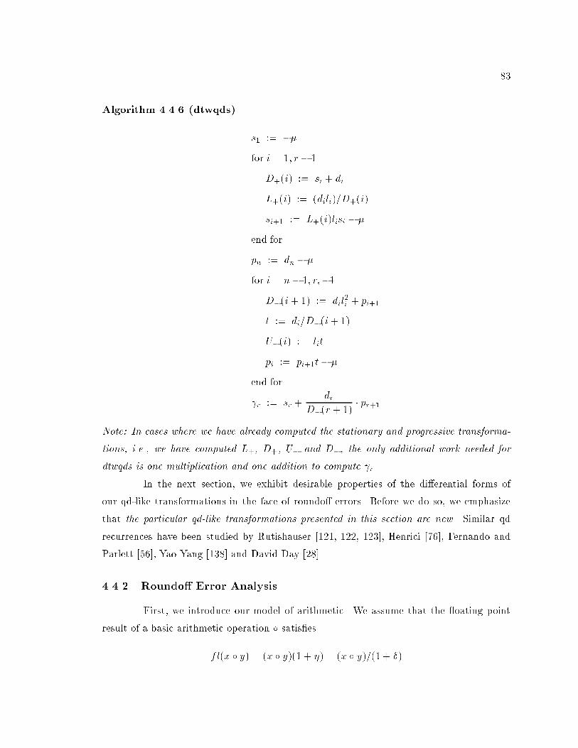
83
Algorithm 4.4.6 (dtwqds)
s1 := ��for i = 1; r� 1
D+(i) := si + di
L+(i) := (dili)=D+(i)
si+1 := L+(i)lisi � �
end for
pn := dn � �
for i = n � 1; r;�1D�(i+ 1) := dil
2i + pi+1
t := di=D�(i+ 1)
U�(i) := lit
pi := pi+1t� �
end for
r := sr +dr
D�(r+ 1)� pr+1
Note: In cases where we have already computed the stationary and progressive transforma-
tions, i.e., we have computed L+, D+, U� and D�, the only additional work needed for
dtwqds is one multiplication and one addition to compute r.
In the next section, we exhibit desirable properties of the di�erential forms of
our qd-like transformations in the face of roundo� errors. Before we do so, we emphasize
that the particular qd-like transformations presented in this section are new. Similar qd
recurrences have been studied by Rutishauser [121, 122, 123], Henrici [76], Fernando and
Parlett [56], Yao Yang [138] and David Day [28].
4.4.2 Roundo� Error Analysis
First, we introduce our model of arithmetic. We assume that the oating point
result of a basic arithmetic operation � satis�es
fl(x � y) = (x � y)(1 + �) = (x � y)=(1 + �)
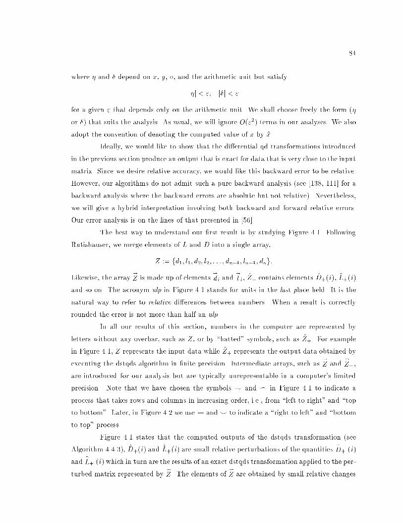
84
where � and � depend on x, y, �, and the arithmetic unit but satisfy
j�j < "; j�j < "
for a given " that depends only on the arithmetic unit. We shall choose freely the form (�
or �) that suits the analysis. As usual, we will ignore O("2) terms in our analyses. We also
adopt the convention of denoting the computed value of x by x.
Ideally, we would like to show that the di�erential qd transformations introduced
in the previous section produce an output that is exact for data that is very close to the input
matrix. Since we desire relative accuracy, we would like this backward error to be relative.
However, our algorithms do not admit such a pure backward analysis (see [138, 111] for a
backward analysis where the backward errors are absolute but not relative). Nevertheless,
we will give a hybrid interpretation involving both backward and forward relative errors.
Our error analysis is on the lines of that presented in [56].
The best way to understand our �rst result is by studying Figure 4.1. Following
Rutishauser, we merge elements of L and D into a single array,
Z := fd1; l1; d2; l2; : : : ; dn�1; ln�1; dng:
Likewise, the array!
Z is made up of elements!
di and!
l i, Z+ contains elements D+(i), L+(i)
and so on. The acronym ulp in Figure 4.1 stands for units in the last place held. It is the
natural way to refer to relative di�erences between numbers. When a result is correctly
rounded the error is not more than half an ulp.
In all our results of this section, numbers in the computer are represented by
letters without any overbar, such as Z, or by \hatted" symbols, such as Z+. For example
in Figure 4.1, Z represents the input data while Z+ represents the output data obtained by
executing the dstqds algorithm in �nite precision. Intermediate arrays, such as!
Z and_
Z+,
are introduced for our analysis but are typically unrepresentable in a computer's limited
precision. Note that we have chosen the symbols ! and _ in Figure 4.1 to indicate a
process that takes rows and columns in increasing order, i.e., from \left to right" and \top
to bottom". Later, in Figure 4.2 we use and^ to indicate a \right to left" and \bottom
to top" process.
Figure 4.1 states that the computed outputs of the dstqds transformation (see
Algorithm 4.4.3), D+(i) and L+(i) are small relative perturbations of the quantities_
D+ (i)
and_
L+ (i) which in turn are the results of an exact dstqds transformation applied to the per-
turbed matrix represented by!
Z. The elements of!
Z are obtained by small relative changes
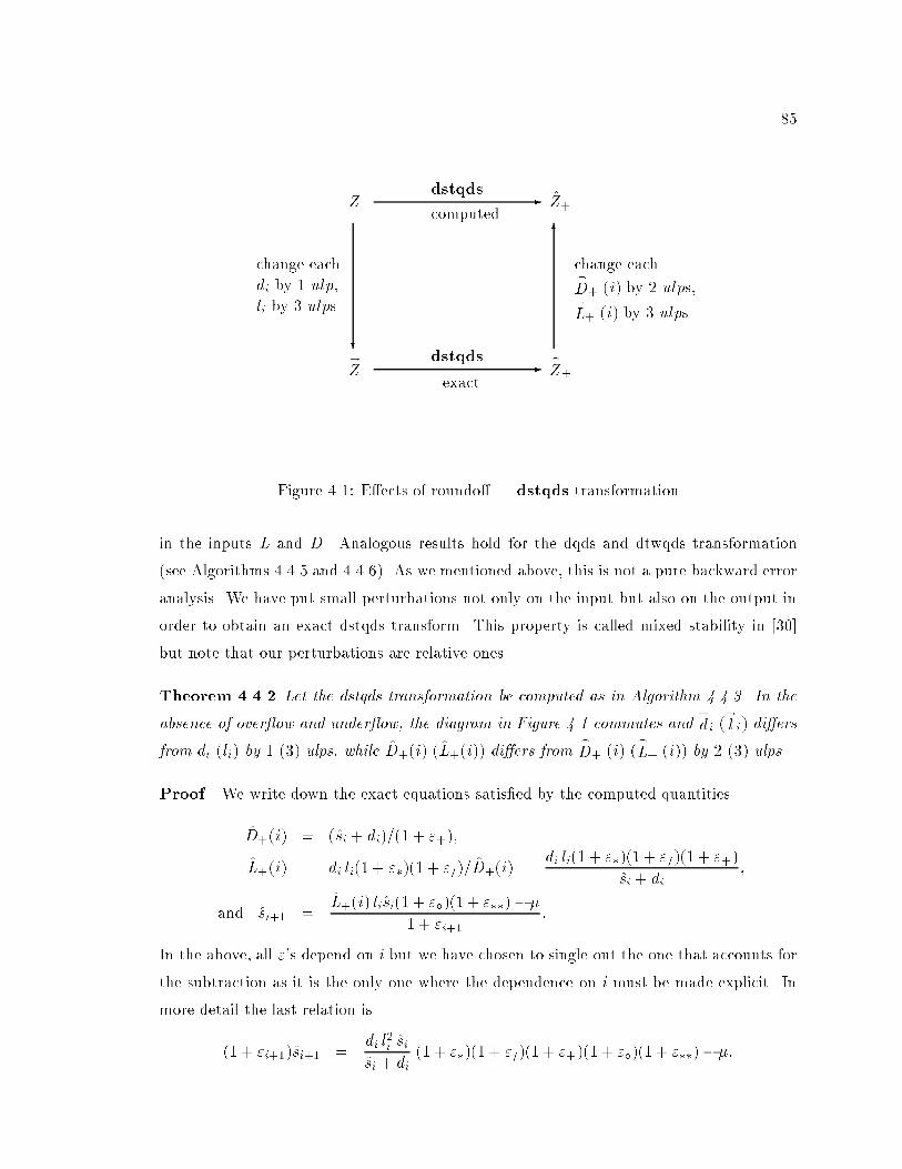
85
-
6
-
?
!
Z_
Z+
Z Z+
dstqds
exact
dstqds
computed
change each
di by 1 ulp,
li by 3 ulps.
change each_
D+ (i) by 2 ulps,_
L+ (i) by 3 ulps.
Figure 4.1: E�ects of roundo� | dstqds transformation
in the inputs L and D. Analogous results hold for the dqds and dtwqds transformation
(see Algorithms 4.4.5 and 4.4.6). As we mentioned above, this is not a pure backward error
analysis. We have put small perturbations not only on the input but also on the output in
order to obtain an exact dstqds transform. This property is called mixed stability in [30]
but note that our perturbations are relative ones.
Theorem 4.4.2 Let the dstqds transformation be computed as in Algorithm 4.4.3. In the
absence of over ow and under ow, the diagram in Figure 4.1 commutes and!
di (!
l i) di�ers
from di (li) by 1 (3) ulps, while D+(i) (L+(i)) di�ers from_
D+ (i) (_
L+ (i)) by 2 (3) ulps.
Proof. We write down the exact equations satis�ed by the computed quantities.
D+(i) = (si + di)=(1 + "+);
L+(i) = di li(1 + "�)(1 + "=)=D+(i) =di li(1 + "�)(1 + "=)(1 + "+)
si + di;
and si+1 =L+(i) lisi(1 + "�)(1 + "��)� �
1 + "i+1:
In the above, all "'s depend on i but we have chosen to single out the one that accounts for
the subtraction as it is the only one where the dependence on i must be made explicit. In
more detail the last relation is
(1 + "i+1)si+1 =di l
2i si
si + di(1 + "�)(1 + "=)(1 + "+)(1 + "�)(1 + "��)� �:
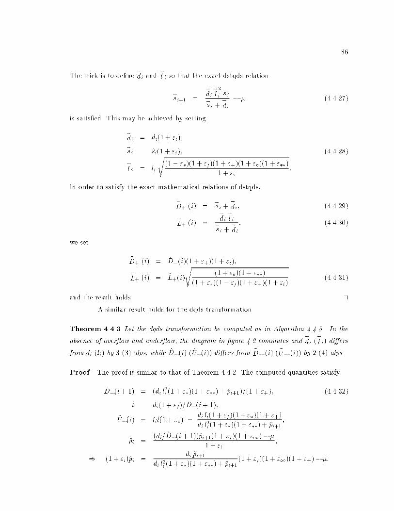
86
The trick is to de�ne!
di and!
l i so that the exact dstqds relation
!
s i+1 =
!
di!
l2
i
!
s i!
s i +!
di� � (4.4.27)
is satis�ed. This may be achieved by setting
!
di = di(1 + "i);
!
s i = si(1 + "i); (4.4.28)
!
l i = li
s(1 + "�)(1 + "=)(1 + "+)(1 + "�)(1 + "��)
1 + "i:
In order to satisfy the exact mathematical relations of dstqds,
_
D+ (i) =!
s i +!
di; (4.4.29)
_
L+ (i) =
!
di!
l i!
s i +!
di; (4.4.30)
we set
_
D+ (i) = D+(i)(1+ "+)(1 + "i);
_
L+ (i) = L+(i)
s(1 + "�)(1 + "��)
(1 + "�)(1 + "=)(1 + "+)(1 + "i)(4.4.31)
and the result holds. tuA similar result holds for the dqds transformation.
Theorem 4.4.3 Let the dqds transformation be computed as in Algorithm 4.4.5. In the
absence of over ow and under ow, the diagram in �gure 4.2 commutes and
di (
l i) di�ers
from di (li) by 3 (3) ulps, while D�(i) (U�(i)) di�ers from^
D� (i) (^
U� (i)) by 2 (4) ulps.
Proof. The proof is similar to that of Theorem 4.4.2. The computed quantities satisfy
D�(i+ 1) = (di l2i (1 + "�)(1 + "��) + pi+1)=(1+ "+); (4.4.32)
t = di(1 + "=)=D�(i+ 1);
U�(i) = lit(1 + "�) =di li(1 + "=)(1 + "�)(1 + "+)
di l2i (1 + "�)(1 + "��) + pi+1
;
pi =(di=D�(i+ 1))pi+1(1 + "=)(1 + "��)� �
1 + "i;
) (1 + "i)pi =di pi+1
di l2i (1 + "�)(1 + "��) + pi+1
(1 + "=)(1 + "��)(1 + "+)� �:
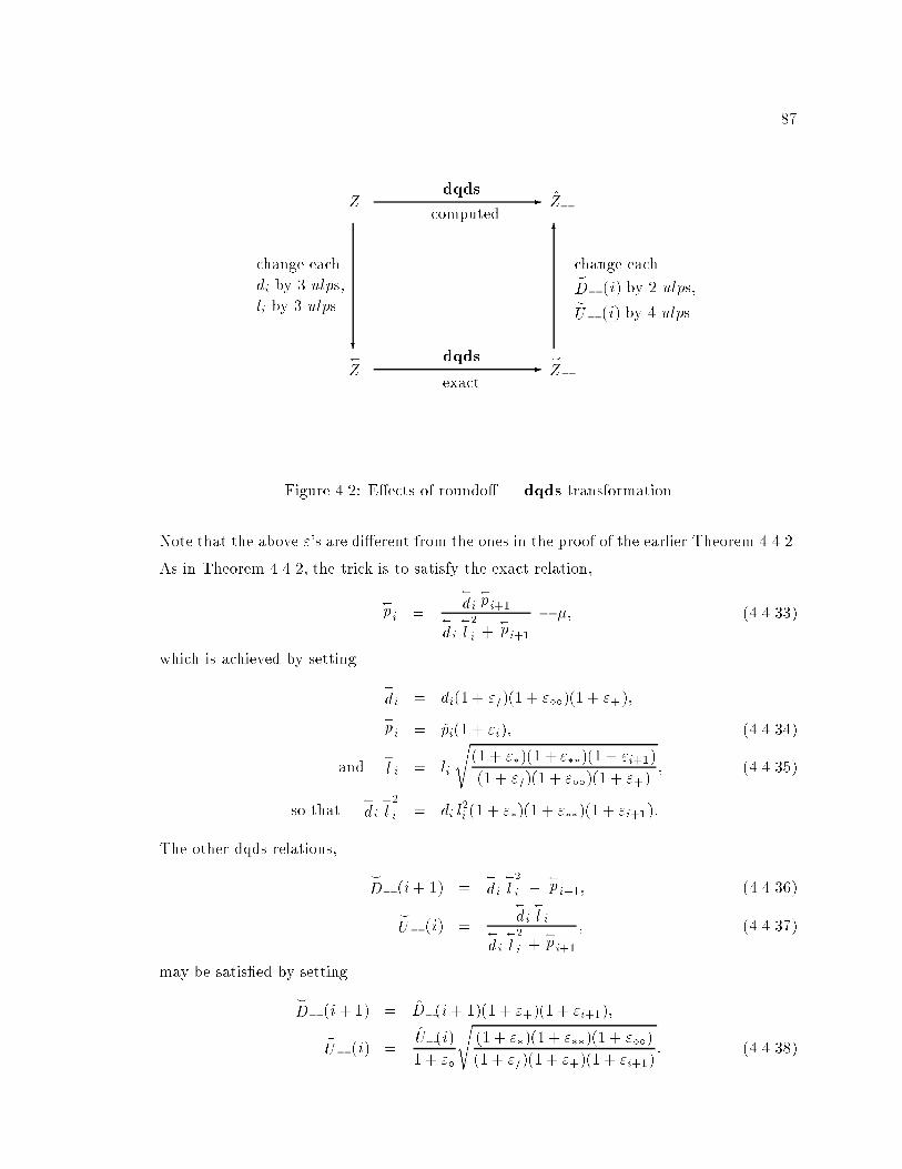
87
-
6
-
?
Z^
Z�
Z Z�
dqds
exact
dqds
computed
change each
di by 3 ulps,
li by 3 ulps.
change each^
D� (i) by 2 ulps,^
U� (i) by 4 ulps.
Figure 4.2: E�ects of roundo� | dqds transformation
Note that the above "'s are di�erent from the ones in the proof of the earlier Theorem 4.4.2.
As in Theorem 4.4.2, the trick is to satisfy the exact relation,
p i =
di
p i+1
d i
l2
i +
pi+1
� �; (4.4.33)
which is achieved by setting
di = di(1 + "=)(1 + "��)(1 + "+);
p i = pi(1 + "i); (4.4.34)
and
l i = li
s(1 + "�)(1 + "��)(1 + "i+1)
(1 + "=)(1 + "��)(1 + "+); (4.4.35)
so that
di
l2
i = di l2i (1 + "�)(1 + "��)(1 + "i+1):
The other dqds relations,
^
D� (i+ 1) =
di
l2
i +
p i+1; (4.4.36)
^
U� (i) =
di
l i
d i
l2
i +
p i+1
; (4.4.37)
may be satis�ed by setting
^
D� (i+ 1) = D�(i+ 1)(1 + "+)(1 + "i+1);
^
U� (i) =U�(i)1 + "�
s(1 + "�)(1 + "��)(1 + "��)(1 + "=)(1 + "+)(1 + "i+1)
: (4.4.38)
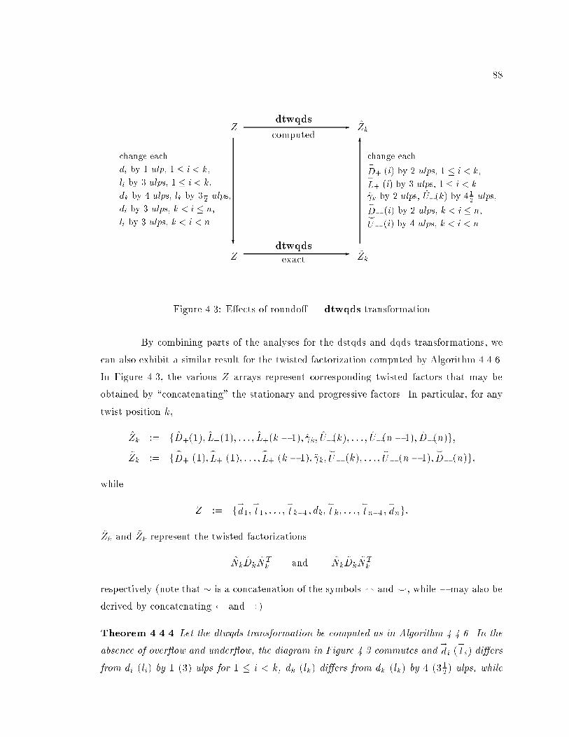
88
-
6
-
?
�Z ~Zk
Z Zk
dtwqds
exact
dtwqds
computed
change each
di by 1 ulp, 1 � i < k,
li by 3 ulps, 1 � i < k,
dk by 4 ulps, lk by 312ulps,
di by 3 ulps, k < i � n,
li by 3 ulps, k < i < n.
change each_
D+ (i) by 2 ulps, 1 � i < k,_
L+ (i) by 3 ulps, 1 � i < k.
~ k by 2 ulps, ~U�
(k) by 412ulps,
^
D�
(i) by 2 ulps, k < i � n,^
U�
(i) by 4 ulps, k < i < n.
Figure 4.3: E�ects of roundo� | dtwqds transformation
By combining parts of the analyses for the dstqds and dqds transformations, we
can also exhibit a similar result for the twisted factorization computed by Algorithm 4.4.6.
In Figure 4.3, the various Z arrays represent corresponding twisted factors that may be
obtained by \concatenating" the stationary and progressive factors. In particular, for any
twist position k,
Zk := fD+(1); L+(1); : : : ; L+(k � 1); k; U�(k); : : : ; U�(n� 1); D�(n)g;~Zk := f_D+ (1);
_
L+ (1); : : : ;_
L+ (k � 1); ~ k;^
U� (k); : : : ;^
U� (n� 1);^
D� (n)g;
while
�Z := f!d1;!
l 1; : : : ;!
l k�1; �dk;
l k; : : : ;
l n�1;
dng:
Zk and ~Zk represent the twisted factorizations
NkDkNTk and ~Nk
~Dk~NTk
respectively (note that � is a concatenation of the symbols _ and ^, while � may also be
derived by concatenating and !).
Theorem 4.4.4 Let the dtwqds transformation be computed as in Algorithm 4.4.6. In the
absence of over ow and under ow, the diagram in Figure 4.3 commutes and!
di (!
l i) di�ers
from di (li) by 1 (3) ulps for 1 � i < k, �dk (�lk) di�ers from dk (lk) by 4 (312) ulps, while
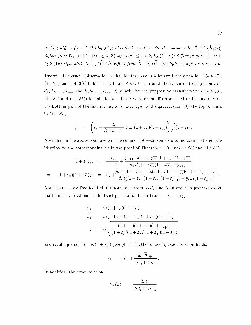
89
di (
l i) di�ers from di (li) by 3 (3) ulps for k < i � n. On the output side, D+(i) (L+(i))
di�ers from_
D+ (i) (_
L+ (i)) by 2 (3) ulps for 1 � i < k, k ( ~U�(k)) di�ers from ~ k ( ~U�(k))
by 2 (412) ulps, while D�(i) (U�(i)) di�ers from^
D� (i) (^
U� (i)) by 2 (4) ulps for k < i � n.
Proof. The crucial observation is that for the exact stationary transformation ( (4.4.27),
(4.4.29) and (4.4.30) ) to be satis�ed for 1 � i � k�1, roundo� errors need to be put only ond1; d2; : : : ; dk�1 and l1; l2; : : : ; lk�1. Similarly for the progressive transformation ((4.4.33),
(4.4.36) and (4.4.37)) to hold for k + 1 � i � n, roundo� errors need to be put only on
the bottom part of the matrix, i.e., on dk+1; : : : ; dn and lk+1; : : : ; ln�1. By the top formula
in (4.4.26),
k =
sk +
dk
D�(k + 1)pk+1(1 + "�
=)(1 + "���)
!�(1 + "k):
Note that in the above, we have put the superscript � on some "'s to indicate that they are
identical to the corresponding "'s in the proof of Theorem 4.4.3. By (4.4.28) and (4.4.32),
(1 + "k) k =
!
sk
1 + "+k+pk+1 � dk(1 + "�= )(1 + "���)(1 + "�+)dk l
2k(1 + "�� )(1 + "���) + pk+1
;
) (1 + "k)(1 + "+k ) k =!
sk +pk+1(1 + "�k+1) � dk(1 + "�= )(1 + "���)(1 + "�+)(1 + "+k )
dk l2k(1 + "�� )(1 + "���)(1 + "�k+1) + pk+1(1 + "�k+1)
:
Note that we are free to attribute roundo� errors to dk and lk in order to preserve exact
mathematical relations at the twist position k. In particular, by setting
~ k = k(1 + "k)(1 + "+k );
�dk = dk(1 + "�= )(1 + "���)(1 + "�+)(1 + "+k );
�lk = lk
vuut (1 + "�� )(1 + "���)(1 + "�k+1)
(1 + "�= )(1 + "���)(1 + "�+)(1 + "+k );
and recalling that
pk= pk(1 + "�k ) (see (4.4.34)), the following exact relation holds,
~ k =!
sk +�dk
pk+1
�dk �l2k+
pk+1:
In addition, the exact relation
~U�(k) =�dk �lk
�dk �l2k+
pk+1
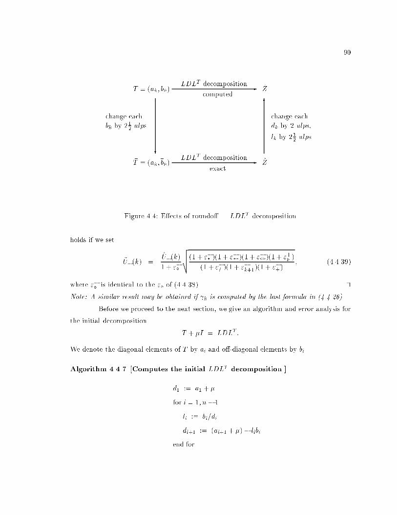
90
-
6
-
?
�T = (ak;�bk) ~Z
T = (ak; bk) Z
LDLT decomposition
exact
LDLT decomposition
computed
change each
bk by 212 ulps.
change each
dk by 2 ulps,
lk by 212 ulps.
Figure 4.4: E�ects of roundo� | LDLT decomposition
holds if we set
~U�(k) =U�(k)1 + "��
vuut(1 + "�� )(1 + "���)(1 + "���)(1 + "+k )
(1 + "�= )(1 + "�k+1)(1 + "�+); (4.4.39)
where "�� is identical to the "� of (4.4.38). tuNote: A similar result may be obtained if k is computed by the last formula in (4.4.26).
Before we proceed to the next section, we give an algorithm and error analysis for
the initial decomposition
T + �I = LDLT :
We denote the diagonal elements of T by ai and o�-diagonal elements by bi.
Algorithm 4.4.7 [Computes the initial LDLT decomposition.]
d1 := a1 + �
for i = 1; n� 1
li := bi=di
di+1 := (ai+1 + �)� libi
end for
91
Theorem 4.4.5 Let the LDLT decomposition be computed as in Algorithm 4.4.7. In the
absence of over ow and under ow, the diagram in Figure 4.4 commutes and �bi di�ers from
bi by 212ulps, while di (li) di�ers from ~di (~li) by 2 (21
2) ulps.
Proof. The computed quantities satisfy
li =bi
di� (1 + "=);
di+1 =(ai+1 + �)=(1 + "+i+1)� bili(1 + "�)
1 + "�i+1;
) (1 + "+i+1)(1 + "�i+1)di+1 = (ai+1 + �)� b2i
di(1 + "=)(1 + "�)(1 + "+i+1):
By setting
~di+1 = di+1(1 + "+i+1)(1 + "�i+1); ~d1 = d1(1 + "+1 );
~li = li
vuut (1 + "�)(1 + "+i+1)
(1 + "=)(1 + "+i )(1 + "�i );
�bi = bi
q(1 + "=)(1 + "�)(1 + "+i+1)(1 + "+i )(1 + "�i ); (4.4.40)
the following exact relations hold
~li =�bi~di;
~di+1 = ai+1 + ���b2i~di:
tuWe can obtain a purely backward error analysis in the above case by showing
that the LDLT decomposition computed by Algorithm 4.4.7 is exact for T + �T , where �T
represents an absolute perturbation in the nonzero elements of T .
Theorem 4.4.6 In the absence of over ow and under ow, the LDLT decomposition com-
puted by Algorithm 4.4.7 is exact for a slightly perturbed matrix T + �T , i.e.,
T + �T + �I = LDLT ;
where
j�bij = j�i1 dili + �i2bij; �i1 ; �i2 < 2:5"; (4.4.41)
j�ai+1j = j�i3 dil2i + �i4 di+1j; �i3 < 3"; �i4 < 2": (4.4.42)
92
Proof. From Theorem 4.4.5, the following relation holds
�T + �I = ~L ~D ~LT ; (4.4.43)
where �T , ~L and ~D are as in Figure 4.4 and Theorem 4.4.5. Equating the diagonal and
o�-diagonal elements of (4.4.43), we get
�bi = ~di~li; (4.4.44)
ai+1 + � = ~di~l2i +
~di+1: (4.4.45)
By Theorem 4.4.5,
~di~li = dili
vuut(1 + "+i )(1 + "�i )(1 + "�)(1 + "+i+1)
1 + "== dili(1 + �i1);
~di~l2i = dil
2i
(1 + "�)(1 + "+i+1)
1 + "== dil
2i (1 + �i3);
~di+1 = di+1(1 + "+i+1)(1 + "�i+1) = di+1(1 + �i4);
where �i1 < 2:5", �i3 < 3" and �i4 < 2". Substituting the above in (4.4.44) and (4.4.45) we
get
bi + (�bi � bi � �i1 dili) = dili;
ai+1 � (�i3 dil2i + �i4 di+1) + � = dil
2i + di+1:
The result now follows by recalling the relation between bi and �bi given in (4.4.40). tuThe backward error given above is small when there is no \element growth" in the
LDLT decomposition. The following lemma proves the well known fact that no element
growth is obtained when factoring a positive de�nite tridiagonal matrix.
Lemma 4.4.1 Suppose ~T is a positive de�nite tridiagonal matrix. Its ~L ~D ~LT factorization,
i.e.,
~T = ~L ~D~LT
satis�es
0 < ~di � ~T(i; i) � k ~Tk; for i = 1; 2; : : : ; n
0 � ~di�1~l2i�1 � ~T (i; i) � k ~Tk; for i = 1; : : : ; n� 1
and ~di~li = ~T (i+ 1; i) ) j ~di~lij � k ~Tk; for i = 1; : : : ; n� 1:
93
Proof. The proof is easily obtained by noting that
~di�1~l2i�1 + ~di = ~T(i; i);
~di~li = ~T(i+ 1; i)
and using properties of a positive de�nite matrix by which the diagonal elements of ~T and
~D must be positive. tuNote that in the above lemma, we do not claim that the elements of ~L are bounded
by k ~Tk. Indeed, the elements of ~L can be arbitrarily large as seen from the following
example, 24 "2p "p
"p 1 + "
35 =
24 1 0
"�p 1
3524 "2p 0
0 "
3524 1 "�p
0 1
35 :
Corollary 4.4.1 Suppose T + �I is a positive de�nite tridiagonal matrix. In the absence
of over ow and under ow, Algorithm 4.4.7 computes L and D such that
T + �T + �I = LDLT ;
where
j�bij < 5"jbij;j�ai+1j < 3"jai+1 + �j;
and since j�j � kTk,
k�Tk1 < 5"kTk1 + 3"j�j < 8"kTk1:
Proof. The result follows by recalling that ~di and ~li are obtained by small relative changes
in di and li respectively, and then substituting the inequalities of Lemma 4.4.1 in (4.4.41)
and (4.4.42). tuNote: The backward error on T is relative if � = 0.
4.4.3 Algorithm X | orthogonality for large relative gaps
In this section, we complete the preliminary version of the method outlined in
Algorithm 4.4.1. It is based on the di�erential qd-like transformations of Section 4.4.1. The
following algorithm computes eigenvectors that are numerically orthogonal whenever the
relative gaps between the eigenvalues of LDLT are large, i.e., O(1).
94
Algorithm X [Computes eigenvectors using bidiagonals.]
1. Find � � kTk such that T + �I is positive (or negative) de�nite.
2. Compute T + �I = LDLT .
3. Compute the eigenvalues, �2j , of LDLT to high relative accuracy (by bisection or the
dqds algorithm [56]).
4. For each computed eigenvalue, � = �2j , do the following
(a) Compute LDLT � �I = L+D+LT+ by the dstqds transform (Algorithm 4.4.3).
(b) Compute LDLT � �I = U�D�UT� by the dqds transform (Algorithm 4.4.5).
(c) Compute k by the top formula of (4.4.26). Pick r such that j rj = mink j kj.(d) Form the approximate eigenvector zj = z
(r)j by solving NrDrN
Tr zj = rer (see
Theorem 3.2.2):
zj(r) = 1;
zj(i) = �L+(i) � zj(i+ 1); i = r � 1; : : : ; 1; (4.4.46)
zj(l+ 1) = �U�(l) � zj(l); l = r; : : : ; n� 1:
(e) If needed, compute znrm = kzjk and set vj = zj=znrm.
tuWe will refer to the above method as Algorithm X in anticipation of Algorithm Y
which will handle the case of small relative gaps.
4.5 Proof of Orthogonality
In this section, we prove that the pairs (�2j ,vj) computed by Algorithm X satisfy
k(T � �2j I)vjk = O(n"kTk); (4.5.47)
jvTj vmj = mink=j;m�1
(O(n")
reldist2(�j ; �k+1)+
O(n")
reldist2(�k; �m)
); j < m; (4.5.48)
where reldist2 is the relative distance as de�ned in Section 4.3 and " is the machine precision.
In particular, the neighboring vectors computed by Algorithm X are such that
jvTj vj+1j =O(n")
reldist2(�j ; �j+1): (4.5.49)
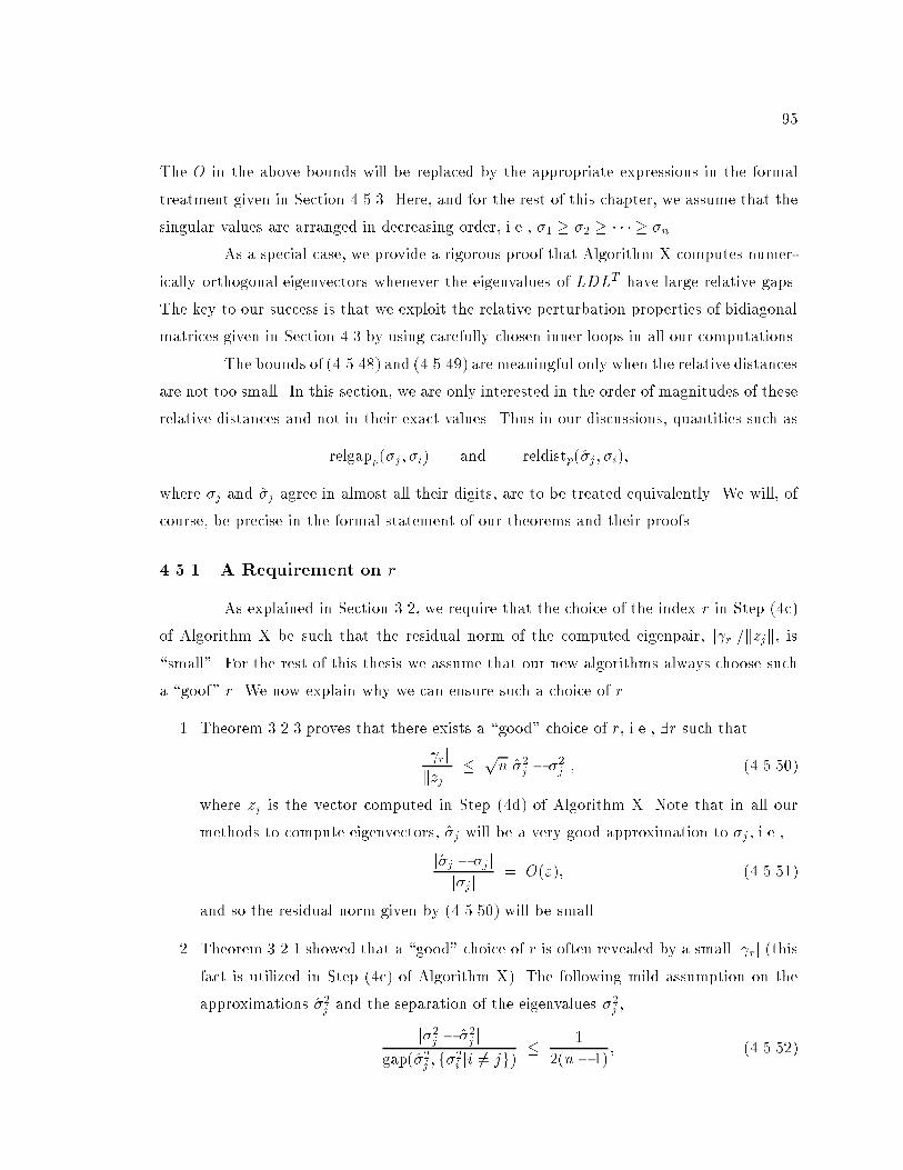
95
The O in the above bounds will be replaced by the appropriate expressions in the formal
treatment given in Section 4.5.3. Here, and for the rest of this chapter, we assume that the
singular values are arranged in decreasing order, i.e., �1 � �2 � � � � � �n.
As a special case, we provide a rigorous proof that Algorithm X computes numer-
ically orthogonal eigenvectors whenever the eigenvalues of LDLT have large relative gaps.
The key to our success is that we exploit the relative perturbation properties of bidiagonal
matrices given in Section 4.3 by using carefully chosen inner loops in all our computations.
The bounds of (4.5.48) and (4.5.49) are meaningful only when the relative distances
are not too small. In this section, we are only interested in the order of magnitudes of these
relative distances and not in their exact values. Thus in our discussions, quantities such as
relgapp(�j ; �i) and reldistp(�j ; �i);
where �j and �j agree in almost all their digits, are to be treated equivalently. We will, of
course, be precise in the formal statement of our theorems and their proofs.
4.5.1 A Requirement on r
As explained in Section 3.2, we require that the choice of the index r in Step (4c)
of Algorithm X be such that the residual norm of the computed eigenpair, j rj=kzjk, is\small". For the rest of this thesis we assume that our new algorithms always choose such
a \goof" r. We now explain why we can ensure such a choice of r.
1. Theorem 3.2.3 proves that there exists a \good" choice of r, i.e., 9r such that
j rjkzjk
� pnj�2j � �2j j; (4.5.50)
where zj is the vector computed in Step (4d) of Algorithm X. Note that in all our
methods to compute eigenvectors, �j will be a very good approximation to �j , i.e.,
j�j � �j jj�j j
= O("); (4.5.51)
and so the residual norm given by (4.5.50) will be small.
2. Theorem 3.2.1 showed that a \good" choice of r is often revealed by a small j rj (thisfact is utilized in Step (4c) of Algorithm X). The following mild assumption on the
approximations �2j and the separation of the eigenvalues �2j ,
j�2j � �2j jgap(�2j ; f�2i ji 6= jg) �
1
2(n� 1); (4.5.52)
96
where gap(�2j ; f�2i ji 6= jg) = mini6=j j�2j � �2i j, ensures that
j rj � 2n � j�2j � �2j j (4.5.53)
(note that we have obtained the above bound by choosing M in Theorem 3.2.1 to
equal 2). Note that kzjk � 1 and so a small value of j rj implies a small residual
norm. Recall that �j will satisfy (4.5.51) and so the eigenvalues have to be very close
together to violate (4.5.52). When the latter happens, there is a theoretical danger
that no k will be small and we shortly see how to handle such a situation. However,
in all our extensive random numerical testing, we have never come across an example
where small gaps cause all 's to be large.
3. We can make a \good" choice of r even in the situation described above by using
twisted Q factorizations that were discussed in Section 3.5. Theorems 3.5.3 and 3.5.4
indicate how to use these factorizations to choose an r that satis�es (4.5.50). Of
course, Step (4c) of Algorithm X needs to be modi�ed when r is not small enough.
For an alternate approach to compute a good r that does not involve orthogonal
factorizations the reader is referred to [42].
In summary, we have seen how to ensure that r is \good" and either (4.5.50)
or (4.5.53) is satis�ed.
Of course, we look for a small residual norm since it implies that the computed
vector is close to the exact eigenvector. The following sin � theorem, see [110, Chapter 11],
is well known and shows that a small residual norm implies a good eigenvector if the
corresponding eigenvalue is isolated. The theorem, which we will often refer to in the next
few sections, is valid for all Hermitian matrices.
Theorem 4.5.1 Let A = A� have an isolated eigenvalue � with normalized eigenvector v.
Consider y, y�y = 1, and real � closer to � than to any other eigenvalue. Then
j sin 6 (v; y)j � kAy � y�k2gap(�)
;
where gap(�) = minfj� � �j : � 6= �; � 2 spectrum (A)g.
The extension of this theorem to higher-dimensional subspaces is due to Davis and
Kahan, see [26] and [27] for more details.
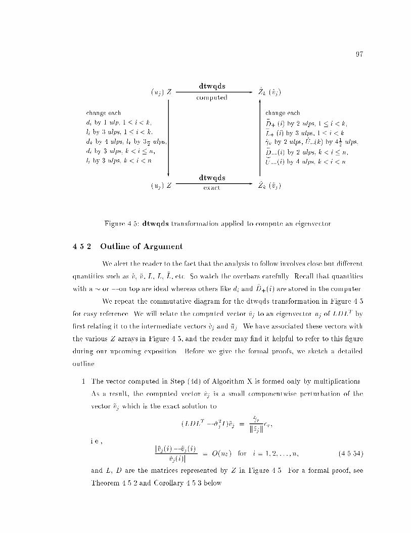
97
-
6
-
?
(�uj) �Z ~Zk (~vj)
(uj) Z Zk (vj)
dtwqds
exact
dtwqds
computed
change each
di by 1 ulp, 1 � i < k,
li by 3 ulps, 1 � i < k,
dk by 4 ulps, lk by 312ulps,
di by 3 ulps, k < i � n,
li by 3 ulps, k < i < n.
change each_
D+ (i) by 2 ulps, 1 � i < k,_
L+ (i) by 3 ulps, 1 � i < k.
~ k by 2 ulps, ~U�
(k) by 412ulps,
^
D�
(i) by 2 ulps, k < i � n,^
U�
(i) by 4 ulps, k < i < n.
Figure 4.5: dtwqds transformation applied to compute an eigenvector
4.5.2 Outline of Argument
We alert the reader to the fact that the analysis to follow involves close but di�erent
quantities such as v, ~v, L, �L, ~L, etc. So watch the overbars carefully. Recall that quantities
with a � or � on top are ideal whereas others like di and D+(i) are stored in the computer.
We repeat the commutative diagram for the dtwqds transformation in Figure 4.5
for easy reference. We will relate the computed vector vj to an eigenvector uj of LDLT by
�rst relating it to the intermediate vectors ~vj and �uj . We have associated these vectors with
the various Z arrays in Figure 4.5, and the reader may �nd it helpful to refer to this �gure
during our upcoming exposition. Before we give the formal proofs, we sketch a detailed
outline.
1. The vector computed in Step (4d) of Algorithm X is formed only by multiplications.
As a result, the computed vector vj is a small componentwise perturbation of the
vector ~vj which is the exact solution to
(�L �D�LT � �2j I)~vj =~ r
k~zjker;
i.e.,jvj(i)� ~vj(i)jj~vj(i)j
= O(n") for i = 1; 2; : : : ; n; (4.5.54)
and �L, �D are the matrices represented by �Z in Figure 4.5. For a formal proof, see
Theorem 4.5.2 and Corollary 4.5.3 below.
98
2. To relate ~vj to an eigenvector �uj of �L �D �LT , we invoke Theorem 4.5.1 to show that
j sin 6 (�uj ; ~vj)j �j~ rj
k~zjk � gap(�2j ; f��2i ji 6= jg) ; (4.5.55)
where gap(�2j ; f��2i ji 6= jg) = mini6=j j�2j � ��2i j, ��2i being the ith eigenvalue of �L �D�LT .
Section 4.5.1 explained how we can always ensure that the residual norm is small, i.e.,
j~ rj=k~zjk = O(n"�2j ). By substituting this value in (4.5.55), the absolute gap turns
into a relative gap and we get
j sin 6 (�uj ; ~vj)j =O(n")
relgap(�j ; f��iji 6= jg) : (4.5.56)
3. Next we relate �uj to an eigenvector uj of LDLT . �L and �D are small componentwise
perturbations of L and D as shown by our roundo� error analysis of the dtwqds
transformation in Theorem 4.4.4. By the properties of a perturbed bidiagonal matrix
�uj can be related to uj (see Corollary 4.3.2), i.e.,
j sin 6 (�uj ; uj)j =O(n")
relgap2(�j ; f��iji 6= jg) : (4.5.57)
The reader should note that the matrices ~L, ~D and �L, �D depend on �2j whereas LDLT
is the �xed representation. By (4.5.54), (4.5.56) and (4.5.57), we have related vectors
computed by Algorithm X to eigenvectors of LDLT ,
j sin 6 (vj ; uj)j =O(n")
relgap2(�j ; f�iji 6= jg) :
Theorem 4.5.3 below contains the details.
Similarly, using the Davis-Kahan Sin� theorem [26, 27] and the subspace theorems
given in Section 4.3, it can be shown that
j sin 6 (vj ; U1:j)j =O(n")
reldist2(�j ; �j+1); (4.5.58)
and j sin 6 (vj ; U j:n)j =O(n")
reldist2(�j ; �j�1); (4.5.59)
where U1:j and U j:n denote the invariant subspaces spanned by u1; u2; : : : ; uj and
uj ; : : : ; un respectively. See Theorems 4.5.4 and 4.5.5 for the details.
4. The dot product between the neighboring vectors vj and vj+1 can now be bounded
since
j cos 6 (vj ; vj+1)j �����cos 6
��
2��6 (vj ; U1:j) + 6 (vj+1; U j+1:n)
������ ;) jvTj vj+1j � j sin 6 (vj ; U1:j)j+ j sin 6 (vj+1; U j+1:n)j:
99
By (4.5.58) and (4.5.59), we get
jvTj vj+1j =O(n")
reldist2(�j ; �j+1):
For details, see Corollary 4.5.2 below. The result (4.5.48) can be shown in the same
way. Hence if all the relative gaps between eigenvalues of LDLT are large, the vectors
computed by Algorithm X are numerically orthogonal.
5. The �nal step in the proof is to show that the residual norms with respect to the
input tridiagonal matrix T are small, i.e., (4.5.47) is satis�ed. Since we can always
ensure a small value of j rj=kzjk, we can show we always compute eigenpairs with
small residual norms, irrespective of the relative gaps. See Theorem 4.5.6 for details.
4.5.3 Formal Proof
Now, the formal analysis begins. We start by showing that the computed vector
is very close to an ideal vector.
Theorem 4.5.2 Let Nr and Dr, ~Nr and ~Dr be the twisted factors represented by Zr and
~Zr respectively in Figure 4.5 (see Theorem 4.4.4 also). Let zj be the value of zj computed
in Step (4d) of Algorithm X, and let ~zj be the exact solution of
~Nr~Dr
~NTr ~zj = ~ rer :
Then zj is a small relative perturbation of ~zj. More speci�cally,
zj(r) = ~zj(r) = 1;
zj(i) = ~zj(i) � (1 + �i); i 6= r; (4.5.60)
where
j�ij �8<: 4(r� i)"; 1 � i < r;
5(i� r)"; r < i � n:(4.5.61)
Proof. Accounting for the rounding error in (4.4.46) of Algorithm X, we get
zj(i) = �L+(i) � zj(i+ 1) � (1 + "i�):
Now replace L+ by_
L+ using (4.4.31) in Theorem 4.4.2 and set i = r � 1 to get
zj(r� 1) = � _
L+ (r� 1) � (1 + �+r�1)zj(r) � (1 + "r�1� ) = ~zj(r� 1) � (1 + �+r�1)(1 + "r�1� );
100
where �+r�1 < 3". Thus (4.5.60) holds for i = r � 1 (note that "r�1� = 0 since zj(r) = 1),
and similarly for i < r� 1. Rounding errors can analogously be attributed to the lower half
of z by
zj(l+ 1) = �U�(l) � zj(l) � (1 + "l+1� ):
Replacing U� by ~U� using (4.4.39) and setting l = r, we obtain
zj(r + 1) = � ~U�(r) � zj(r) � (1 + ��r+1)(1 + "r+1� ) = ~zj(r � 1) � (1 + ��r+1)(1 + "r+1� );
where ��r+1 < 4:5". Thus (4.5.60) holds for i = r + 1 (note that "r+1� = 0), and by
using (4.4.38) we can similarly show that it holds for i > r + 1. tuThe following theorem is at the heart of the results of this section.
Theorem 4.5.3 Let (�2j ; uj) denote the jth eigenpair of LDLT , and let �2j be the approx-
imation used to compute zj = z(r)j by Step (4d) of Algorithm X, where r is an index such
thatj~ rjk~zjk
� pn j�2j � ��2j j: (4.5.62)
Then
j sin 6 (zj ; uj)j � 5n"+
pn j�2j � ��2j j
gap(�2j ; f��2i ji 6= jg) +3n"
relgap2(�j ; f��iji 6= jg);
where ��i2 is the ith eigenvalue of �L �D�LT (see Figure 4.5) and di�ers from �2i by a few ulps.
Proof. As we outlined in Section 4.5.2, to prove this result we will relate zj to uj by �rst re-
lating zj to an eigenvector of the intermediate matrix �L �D�LT (see Figure 4.5). Theorem 4.5.2
links zj to ~zj and implies that
j sin 6 (zj ; ~zj)j � kzj � ~zjk � 5n": (4.5.63)
Note that ~zj is the exact solution to
(�L �D �LT � �2j I)~zj = ~ rer:
Let (��2j ,�uj) denote the jth eigenpair of �L �D�LT . By Theorem 4.5.1,
j sin 6 (~zj ; �uj)j �j~ rj
k~zjk � gap(�2j ; f��2i ji 6= jg) :
101
Since r is such that (4.5.62) is satis�ed (recall that Section 4.5.1 explains why this bound
can always be satis�ed), we get
j sin 6 (~zj ; �uj)j �pn j�2j � ��2j j
gap(�2j ; f��2i ji 6= jg) : (4.5.64)
Since �L and �D are small relative perturbations of L andD, ��i is a small relative perturbation
of �i by Corollary 4.3.1. In addition,
j sin 6 (�uj ; uj)j �3n"
relgap2(�j ; f��iji 6= jg); (4.5.65)
where we obtained the above bound by converting all the ulp changes in entries of L and
D given in Theorem 4.4.4 to ulp changes in the o�-diagonal and diagonal elements of
LD1=2, and then applying Corollary 4.3.2. The result now follows from (4.5.63), (4.5.64)
and (4.5.65) since
j sin 6 (zj ; uj)j � j sin 6 (zj ; ~zj)j+ j sin 6 (~zj ; �uj)j+ j sin 6 (�uj ; uj)j:
tuWe can generalize the above result to bound the angle between the computed vector and
the invariant subspaces of LDLT .
Theorem 4.5.4 Let �2j be the approximation used to compute zj by Step (4d) of Algo-
rithm X, and r be such that (4.5.62) is satis�ed. Let (�2j ; uj) be the jth eigenpair of LDLT
and let U1:k denote the subspace spanned by u1; : : : ; uk. Then for j � k < n,
j sin 6 (zj ; U1:k)j � 5n"+
pn j�2j � ��2j j
gap(�2j ; f��2k+1g)+
3n"
relgap2(�j ; f��k+1g);
where ��i2 is the ith eigenvalue of �L �D�LT (see Figure 4.5) and di�ers from �2i by a few ulps.
Proof. The proof is almost identical to that of the above Theorem 4.5.3 except that
instead of applying Theorem 4.5.1 and Corollary 4.3.2 to get bounds on the angles between
individual vectors, we apply the Davis-Kahan Sin� Theorem [26, 27] and Corollary 4.3.3
to get similar bounds on the angles between corresponding subspaces. tu
Theorem 4.5.5 Let �2j be the approximation used to compute zj by Step (4d) of Algo-
rithm X, and r be such that (4.5.62) is satis�ed. Let (�2j ; uj) be the jth eigenpair of LDLT
and let Uk:n denote the subspace spanned by uk ; : : : ; un. Then for 1 < k � j,
j sin 6 (zj ; Uk:n)j � 5n" +
pn j�2j � ��2j j
gap(�2j ; f��2k�1g)+
3n"
relgap2(�j ; f��k�1g);
where ��i2 is the ith eigenvalue of �L �D�LT (see Figure 4.5) and di�ers from �2i by a few ulps.
102
Finally we can bound the dot products between the computed eigenvectors using the above
results.
Corollary 4.5.1 Let �2j and �2m be the approximations used to compute zj and zm respec-
tively by Step (4d) of Algorithm X. Let the twist indices r for both these computations
satisfy (4.5.62). Then
jzTj zm)jkzjk � kzmk
� 10n"+ mink=j;m�1
( pn j�2j � ��2j j
gap(�2j ; f��2k+1g)+
pn j�2m � ��2mj
gap(�2m; f��2kg)+
3n"
relgap2(�j ; f��k+1g)+
3n"
relgap2(�m; f��kg)
); for j < m:
where ��i2 is the ith eigenvalue of �L �D�LT (see Figure 4.5) and di�ers from �2i by a few ulps.
Proof. The cosine of the angle between the computed vectors can be bounded by
j cos 6 (zj ; zm)j �����cos 6
��
2��6 (zj ; U1:k) + 6 (zm; Uk+1:n)
������= j sin 6 (zj ; U1:k)j+ j sin 6 (zm; Uk+1:n)j;
where U1:k and Uk+1:n are as in Theorems 4.5.4 and 4.5.5. The result now follows by
applying the results of these theorems, and then choosing k to be the index where the
bound is minimum. tu
Corollary 4.5.2 Let �2j and �2j+1 be the approximations used to compute zj and zj+1 re-
spectively by Step (4d) of Algorithm X. Let the indices r for both these computations sat-
isfy (4.5.62). Then
jzTj zj+1)jkzjk � kzj+1k
� 10n"+
pn j�2j � ��2j j
gap(�2j ; f��2j+1g)+
pn j�2j+1 � ��2j+1j
gap(�2j+1; f��2j g)+
3n"
relgap2(�j ; f��j+1g)+
3n"
relgap2(�j+1; f��jg):
where ��i2 is the ith eigenvalue of �L �D�LT (see Figure 4.5) and di�ers from �2i by a few ulps.
Proof. This is a special case of Corollary 4.5.1. tuInstead of assuming (4.5.62), if we assume that
j~ rj � 2n � j�2j � ��2j j; (4.5.66)
we get a bound that is weaker by a factor of only 2pn. If such an index r is chosen
in Algorithm X, we can modify the middle terms in Corollaries 4.5.1 and 4.5.2 by using
103
the above bound. See Section 4.5.1 to see how we can ensure that either one of (4.5.62)
or (4.5.66) is satis�ed.
Since we can compute the singular values of a bidiagonal matrix to high relative
accuracy, we can �nd �j such that
j�2j � �2j j � h(n) � " � �2j (4.5.67)
where h is a slowly growing function of n.
For the sake of completeness, we prove the well known fact that normalizing zj , as
in Step (4e) of Algorithm X, does not change the accuracy of the computed eigenvectors.
Corollary 4.5.3 Let zj and ~zj be as in Theorem 4.5.2. Let ~vj = ~zj=k~zjk, and vj be the
computed value of zj=kzjk (see Step (4e) of Algorithm X). Then
vj(i) = ~vj(i) � (1 + "i); (4.5.68)
where j"ij � (n+ 2)"+ j�ij+ maxi j�ij, and �i is as in (4.5.61).
Proof. The computed value of kzjk equals kzjk � (1 + "k) where j"kj < (n+ 1)". Thus
vj(i) =zj(i)
kzjk� 1 + "=
1 + "k: (4.5.69)
By (4.5.60) of Theorem 4.5.2,
kzjk =
nXi=1
~zj(i)2 � (1 + �i)
2
!1=2
= k~zjk X
i
~zj(i)2
k~zjk2� (1 + �i)
2
!1=2
:
It follows that
kzjk = k~zjk � (1 + �max); where j�maxj = maxij�ij: (4.5.70)
Substituting (4.5.60) and (4.5.70) in (4.5.69), we get
vj(i) =~zj(i)
k~zjk� (1 + "=)(1 + �i)
(1 + "k)(1 + �max);
and the result follows. tuThus for the eigenpairs computed by Algorithm X, the following result holds.
Corollary 4.5.4 Let (�2j ; vj) be the approximate eigenpairs computed by Algorithm X. As-
suming that (4.5.66) holds,
jvTj vj+1)j � 22n"+2nj�2j � ��2j j
gap(�2j ; f��2j+1g)+2nj�2j+1 � ��2j+1jgap(�2j+1; f��2j g)
+
3n"
relgap2(�j ; f��j+1g)+
3n"
relgap2(�j+1; f��jg); (4.5.71)
104
and by the relative accuracy of �2j (see (4.5.67)),
jvTj vj+1)j � 22n"+2nh(n)"
relgap(�2j ; f��2j+1g)+
2nh(n)"
relgap(�2j+1; f��2jg)+
3n"
relgap2(�j ; f��j+1g)+
3n"
relgap2(�j+1; f��jg): (4.5.72)
where ��i2 is the ith eigenvalue of �L �D�LT (see Figure 4.5) and di�ers from �2i by a few ulps.
Note that we have chosen to exhibit the result in two forms, namely, (4.5.71) and
(4.5.72). The di�erence is in the second and third terms of the two bounds. Since we only
care about each term in the bound being O("), often it may not be necessary to �nd an
eigenvalue to full relative accuracy. For example, suppose �2n = " and �2n�1 = 1, then there
is no need to �nd all the correct digits of �2n. Instead, absolute accuracy will su�ce and be
more e�cient in such a case. The �rst result (4.5.71) makes this clear.
We now show that irrespective of the relative gaps, Algorithm X always computes
eigenpairs with small residual norms.
Theorem 4.5.6 Let T + �I be a positive de�nite tridiagonal matrix and let (�2j ,vj) be the
approximate eigenpairs computed by Algorithm X. Then their residual norms are small, i.e.,
for j = 1; 2; : : : ; n,
k(T + �I � �2j I)vjk ��2kTk1(2nh(n) + 11n3=2+ 4) + 48
�� "; (4.5.73)
assuming that (4.5.66) holds.
Proof. We refer the reader to Figure 4.5 for notation used in this proof. Recall that by
de�nition the vector ~vj is the exact solution to
(�L �D�LT � �2j I)~vj =~ r
k~zker: (4.5.74)
The elements of �L and �D are small relative perturbations of the elements of L and D. In
particular,
�di = di(1 + �i1); (4.5.75)
�di�li = dili(1 + �i2) (4.5.76)
�di�l2i = dil
2i (1 + �i3) (4.5.77)
where
j�i1j < 4"; j�i2j < 3:5"; and j�i3j < 5" (4.5.78)
105
(these bounds on �i's can be deduced from Theorems 4.4.2, 4.4.3 and 4.4.4). Consider the
ith equation of (4.5.74),
�di�1�li�1~vj(i� 1) + ( �di�1�l2i�1 + �di � �2j )~vj(i) +�di�li~vj(i+ 1) = Ki;
where Ki = 0 if i 6= r and Kr = ~ r=k~zk. Substituting (4.5.68), (4.5.75), (4.5.76) and (4.5.77)into the above equation, we get
di�1li�1vj(i� 1) + (di�1l2i�1 + di � �2j )vj(i) + dilivj(i+ 1) = Ki + �i;
where
j�ij < j"i�1di�1li�1j+ j"ij � (jdi�1l2i�1j+ jdij) + j"i+1dilij) +j�i�12 ~vj(i� 1)j+ (j�i�13 j+ j�i1j) � j~vj(i)j+ j�i2~vj(i+ 1)j:
In the above, the "i's are as in (4.5.68). Since j"ij < 11n" and by (4.5.78), we can bound �i
by
j�ij < 11n" � kLDLTk1 + 16" �maxf~vj(i� 1); ~vj(i); ~vj(i+ 1)g:
Thus
(LDLT � �2j I)vj = rj : (4.5.79)
Substituting the bound for j rj from (4.5.66), we get
krjk < (2nh(n)�2j + 11n3=2kLDLTk1 + 48) � " <�(2nh(n) + 11n3=2)kLDLTk1 + 48
�� ":
By the backward stability of the Cholesky factorization (see Corollary 4.4.1),
T + �T + �I = LDLT ; (4.5.80)
where k�Tk1 � 8"kTk1. From (4.5.79) and (4.5.80),
(T + �I � �2j I)vj = (LDLT � �2j I � �T )vj = rj � �T � vj ;
and the result follows since kLDLTk1 � 2kTk1 (recall that j�j � kTk). tu
4.5.4 Discussion of Error Bounds
The careful reader may worry about the nh(n) and n3=2 terms in the bounds on the
residual norms of (4.5.73), and the nh(n) term in the dot product bound given by (4.5.72).
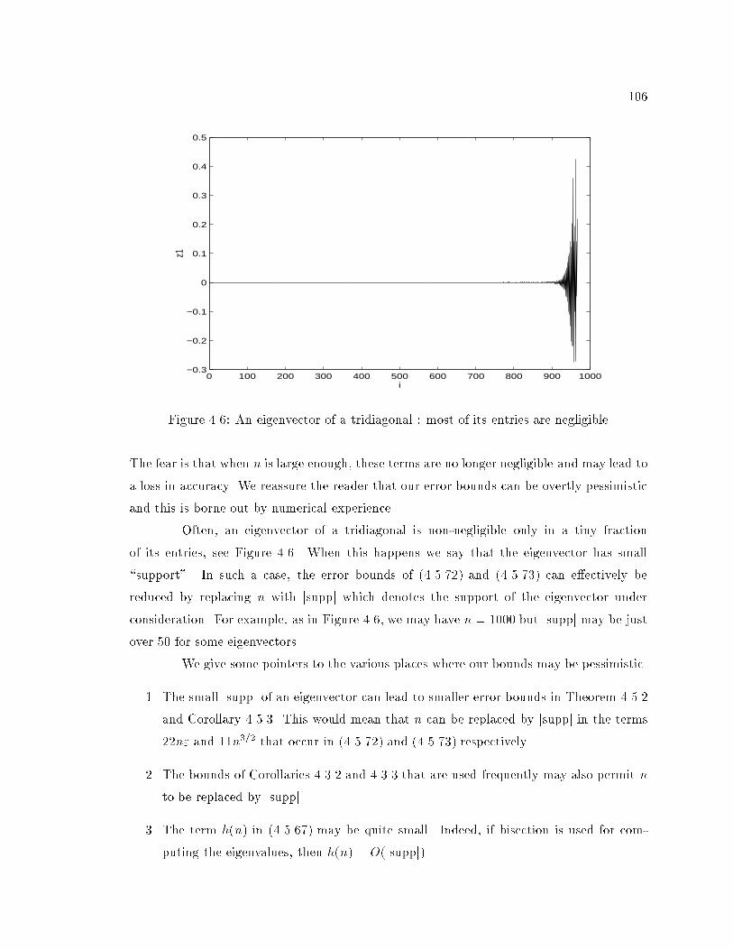
106
0 100 200 300 400 500 600 700 800 900 1000−0.3
−0.2
−0.1
0
0.1
0.2
0.3
0.4
0.5
i
z1
Figure 4.6: An eigenvector of a tridiagonal : most of its entries are negligible
The fear is that when n is large enough, these terms are no longer negligible and may lead to
a loss in accuracy. We reassure the reader that our error bounds can be overtly pessimistic
and this is borne out by numerical experience.
Often, an eigenvector of a tridiagonal is non-negligible only in a tiny fraction
of its entries, see Figure 4.6. When this happens we say that the eigenvector has small
\support". In such a case, the error bounds of (4.5.72) and (4.5.73) can e�ectively be
reduced by replacing n with jsuppj which denotes the support of the eigenvector under
consideration. For example, as in Figure 4.6, we may have n = 1000 but jsuppj may be justover 50 for some eigenvectors.
We give some pointers to the various places where our bounds may be pessimistic.
1. The small jsuppj of an eigenvector can lead to smaller error bounds in Theorem 4.5.2
and Corollary 4.5.3. This would mean that n can be replaced by jsuppj in the terms
22n" and 11n3=2 that occur in (4.5.72) and (4.5.73) respectively.
2. The bounds of Corollaries 4.3.2 and 4.3.3 that are used frequently may also permit n
to be replaced by jsuppj.
3. The term h(n) in (4.5.67) may be quite small. Indeed, if bisection is used for com-
puting the eigenvalues, then h(n) = O(jsuppj).
107
4. Thepn term in (4.5.62) is really k~vjk�11 (see Theorem 3.2.3) and can be O(1) if the
largest entry of the normalized eigenvector is O(1). Consequently, our results will be
more accurate than as suggested by our error bounds.
4.5.5 Orthogonality in Extended Precision Arithmetic
Suppose the user wants d digits of accuracy, i.e., residual norms and dot products
of about 10�d are acceptable. Until now, we have implicitly assumed that the arithmetic
precision in which we compute is identical to the acceptable level of accuracy, e.g., we desire
O(") accuracy in our goals of (1.1.1) and (1.1.2) where " is the precision of the arithmetic.
Can a desired level of accuracy by guaranteed by arithmetic of a higher precision? For
example, the user may want single precision accuracy when computing in double precision,
or we may aim for double precision accuracy by computing in quadruple precision arithmetic.
The IEEE standard also speci�es a Double-Extended precision format (sometimes referred
to as \80-bit" arithmetic) and on some machines, these extra precise computations may
be performed in hardware [2, 65]. Quadruple precision arithmetic is generally simulated in
software [91, 120].
In order to get single precision accuracy, we may try and execute Algorithm X in
double precision arithmetic. However, there are cases when this simple strategy will not
work. Consider Wilkinson's matrix W+21 where the largest pair of eigenvalues agree to more
than 16 digits (see [136, p.309] for more details). By the theory developed in Section 4.5,
the corresponding eigenvectors computed by Algorithm X can be nearly parallel even if we
compute in double precision! And indeed in a numerical run, we observe large dot products.
Thus we cannot use the doubled precision accuracy in a naive manner.
We now indicate without proof that Algorithm X can easily be modi�ed to deliver
results that are accurate to a desired accuracy when operating in arithmetic of doubled
precision, i.e., by slightly modifying Algorithm X, it almost always delivers eigenpairs
with O(p") residual norms and dot products when using arithmetic of precision
". The modi�cation is that after computing the LDLT decomposition in Step 2 of Algo-
rithm X, random componentwise perturbations of O(p") should be made in the elements
of L and D. This perturbation makes it unlikely that relative gaps between the eigenvalues
of the perturbed LDLT will be smaller than O(p"). In many cases, the above e�ect can
be achieved just by performing the computation to get the LDLT decomposition inp"
precision arithmetic. The computation of the eigenvalues and eigenvectors by Steps 3 and 4
108
of Algorithm X must, of course, be performed in the doubled precision. The results of
Theorem 4.5.6 and Corollary 4.5.4 now imply that both residual norms and dot products
are O(p").
4.6 Numerical Results
We now provide numerical evidence to verify our claims of the last two sections.
We consider two types of matrices with the following distribution of eigenvalues.
Type 1. n�1 eigenvalues uniformly distributed from " to (n�1)", and the nth eigenvalueat 1, i.e.,
�i = i � "; i = 1; 2; : : : ; n� 1; and �n = 1:
Type 2. One eigenvalue at ", n � 2 eigenvalues uniformly distributed from 1 +p" to
1 + (n� 2)p", and the last eigenvalue at 2, i.e.,
�1 = "; �i = 1 + (i� 1) � p"; i = 2; : : : ; n� 1; and �n = 2:
We generated matrices of the above type using the LAPACK test matrix genera-
tor [36], which �rst forms a random dense symmetric matrix with the given spectrum and
Householder reduction of this dense matrix then yields a tridiagonal of the desired type.
In Table 4.1, we compare the times taken by our new algorithm with the LAPACK
and EISPACK implementations of inverse iteration on matrices of type 1. The O(n3)
behavior of the LAPACK and EISPACK codes is seen in this table while Algorithm X takes
O(n2) time. We see that Table 4.1 shows the new algorithm to be consistently faster | it
is about 3 times faster on a matrix of size 50 and nearly 23 times faster on a 1000� 1000
matrix. As we proved in the last section, Algorithm X delivers vectors that are numerically
orthogonal, and this is seen in Table 4.2.
On matrices of type 2, our theory predicts that the vectors we compute will have
dot products of aboutp" (see Corollary 4.5.4). Indeed, as Table 4.3 shows, that is what
we observe. The times taken by Algorithm X to compute the vectors in this case are
approximately the same as the times listed in Table 4.1. Vectors that have dot products
of O(p") are sometimes referred to as a semi-orthogonal basis. In some cases, such a basis
may be as good as an orthogonal basis, see [114].

109
Matrix Time(LAPACK) Time(EISPACK) Time(Alg. X) Time(Alg. X) /
Size (in s.) (in s.) (in s.) Time(LAPACK)
50 0:10 0:09 0:03 3:33
100 0:45 0:34 0:07 6:43
250 3:60 2:32 0:37 9:73
500 19:88 11:21 1:35 14:73
750 57:53 29:65 2:98 19:31
1000 124:98 60:81 5:51 22:68
Table 4.1: Timing results on matrices of type 1
Matrix maxi kT vi � �2i vik maxi6=j jvTi vj jSize LAPACK EISPACK Alg. X LAPACK EISPACK Alg. X
50 1:6 � 10�16 5:9 � 10�15 1:2 � 10�16 1:1 � 10�15 2:8 � 10�15 2:5 � 10�15100 3:1 � 10�17 1:5 � 10�15 1:3 � 10�17 1:1 � 10�15 5:7 � 10�15 2:0 � 10�15250 1:1 � 10�16 2:1 � 10�14 1:1 � 10�16 1:7 � 10�15 1:4 � 10�14 1:5 � 10�14500 1:1 � 10�16 4:9 � 10�14 5:5 � 10�18 3:5 � 10�15 2:0 � 10�14 4:2 � 10�14750 1:1 � 10�16 3:6 � 10�14 3:2 � 10�18 4:6 � 10�15 3:9 � 10�14 4:1 � 10�141000 1:2 � 10�17 5:1 � 10�14 2:2 � 10�16 4:4 � 10�15 6:0 � 10�14 8:3 � 10�14
Table 4.2: Accuracy results on matrices of type 1
Matrix Size maxi kT vi � �2i vik maxi6=j jvTi vj j50 7:2 � 10�16 5:2 � 10�9100 1:0 � 10�15 3:9 � 10�9250 1:5 � 10�16 2:5 � 10�9500 2:1 � 10�15 2:1 � 10�9750 2:6 � 10�15 2:4 � 10�91000 2:9 � 10�15 1:7 � 10�9
Table 4.3: Accuracy results on matrices of type 2
110
A nice property of Algorithm X is that the dot products of the vectors computed
can be predicted quite accurately, based solely on the relative separation of the eigenvalues.
As exhibited in Sections 2.8 and 4.2, existing implementations do not have such a property.
This feature is useful when larger dot products are acceptable, such as in the case of semi-
orthogonal vectors.
Algorithm X is a major step in obtaining an O(n2) algorithm for the symmetric
tridiagonal problem. However, it does not always deliver vectors that are numerically
orthogonal. In the next chapter, we investigate how to extend Algorithm X in order to
always achieve the desired accuracy while doing only O(n2) work.
111
Chapter 5
Multiple Representations
In the previous chapter, we saw how to obtain vectors that are guaranteed to
be numerically orthogonal when eigenvalues have large relative gaps. In this chapter and
the next, we concentrate our energies on the case when relative gaps are smaller than a
threshold, say 1=n. Such eigenvalues will be called a cluster throughout this chapter.
The following is our plan of attack:
1. In Section 5.1, we present two examples which suggest that orthogonality may be
achieved by shifting the matrix close to a cluster and then forming a bidiagonal factor-
ization of the shifted matrix. The aim is to clearly distinguish between the individual
eigenvalues of the cluster so that we can treat each eigenvalue as isolated and compute
the corresponding eigenvector as before. If the bidiagonal factorization is \good", the
computed vectors will be nearly orthogonal.
2. In Section 5.2, we list the properties that a \good" bidiagonal factorization must
satisfy. We call such a factorization a relatively robust representation. Section 5.2.1
introduces relative condition numbers that indicate when a representation is relatively
robust. In Section 5.2.3, we investigate factorizations of nearly singular tridiagonal
matrices and attempt to explain why these representations are almost always relatively
robust.
3. In Section 5.3, we explain why the vectors computed using di�erent relatively robust
representations turn out to be numerically orthogonal. We do so by introducing a
representation tree which we use as a visual tool for our exposition. A representation
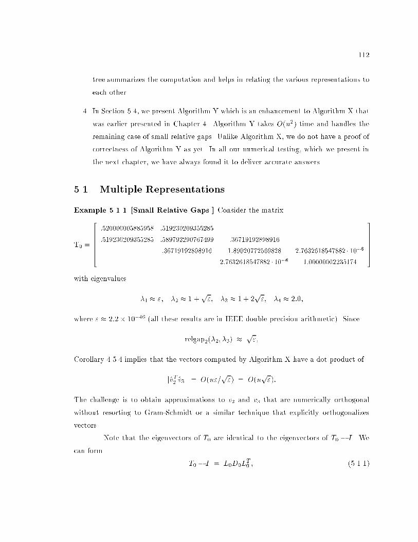
112
tree summarizes the computation and helps in relating the various representations to
each other.
4. In Section 5.4, we present Algorithm Y which is an enhancement to Algorithm X that
was earlier presented in Chapter 4. Algorithm Y takes O(n2) time and handles the
remaining case of small relative gaps. Unlike Algorithm X, we do not have a proof of
correctness of Algorithm Y as yet. In all our numerical testing, which we present in
the next chapter, we have always found it to deliver accurate answers.
5.1 Multiple Representations
Example 5.1.1 [Small Relative Gaps.] Consider the matrix
T0 =
2666664
:520000005885958 :519230209355285
:519230209355285 :589792290767499 :36719192898916
:36719192898916 1:89020772569828 2:7632618547882 � 10�8
2:7632618547882 � 10�8 1:00000002235174
3777775
with eigenvalues
�1 � "; �2 � 1 +p"; �3 � 1 + 2
p"; �4 � 2:0;
where " � 2:2� 10�16 (all these results are in IEEE double precision arithmetic). Since
relgap2(�2; �3) �p";
Corollary 4.5.4 implies that the vectors computed by Algorithm X have a dot product of
jvT2 v3j = O(n"=p") = O(n
p"):
The challenge is to obtain approximations to v2 and v3 that are numerically orthogonal
without resorting to Gram-Schmidt or a similar technique that explicitly orthogonalizes
vectors.
Note that the eigenvectors of T0 are identical to the eigenvectors of T0 � I . We
can form
T0 � I = L0D0LT0 ; (5.1.1)
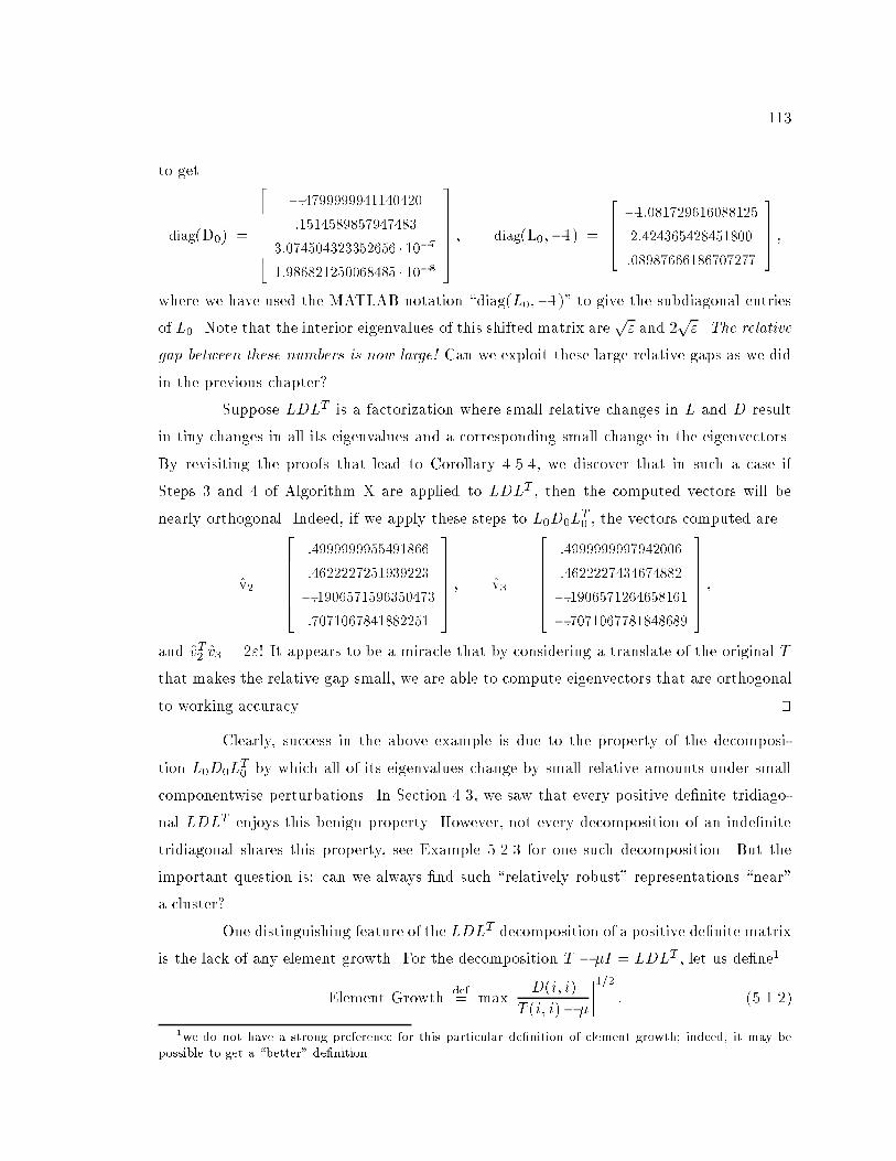
113
to get
diag(D0) =
2666664
�:4799999941140420
:1514589857947483
3:074504323352656 � 10�7
1:986821250068485 � 10�8
3777775 ; diag(L0;�1) =
2664�1:081729616088125
2:424365428451800
:08987666186707277
3775 ;
where we have used the MATLAB notation \diag(L0;�1)" to give the subdiagonal entriesof L0. Note that the interior eigenvalues of this shifted matrix are
p" and 2
p". The relative
gap between these numbers is now large! Can we exploit these large relative gaps as we did
in the previous chapter?
Suppose LDLT is a factorization where small relative changes in L and D result
in tiny changes in all its eigenvalues and a corresponding small change in the eigenvectors.
By revisiting the proofs that lead to Corollary 4.5.4, we discover that in such a case if
Steps 3 and 4 of Algorithm X are applied to LDLT , then the computed vectors will be
nearly orthogonal. Indeed, if we apply these steps to L0D0LT0 , the vectors computed are
v2 =
2666664
:4999999955491866
:4622227251939223
�:1906571596350473
:7071067841882251
3777775 ; v3 =
2666664
:4999999997942006
:4622227434674882
�:1906571264658161
�:7071067781848689
3777775 ;
and vT2 v3 = 2"! It appears to be a miracle that by considering a translate of the original T
that makes the relative gap small, we are able to compute eigenvectors that are orthogonal
to working accuracy. tu
Clearly, success in the above example is due to the property of the decomposi-
tion L0D0LT0 by which all of its eigenvalues change by small relative amounts under small
componentwise perturbations. In Section 4.3, we saw that every positive de�nite tridiago-
nal LDLT enjoys this benign property. However, not every decomposition of an inde�nite
tridiagonal shares this property, see Example 5.2.3 for one such decomposition. But the
important question is: can we always �nd such \relatively robust" representations \near"
a cluster?
One distinguishing feature of the LDLT decomposition of a positive de�nite matrix
is the lack of any element growth. For the decomposition T � �I = LDLT , let us de�ne1
Element Growthdef= max
���� D(i; i)
T (i; i)� �
����1=2
: (5.1.2)
1we do not have a strong preference for this particular de�nition of element growth; indeed, it may be
possible to get a \better" de�nition
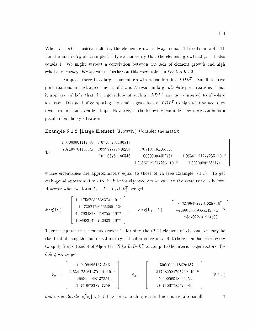
114
When T � �I is positive de�nite, the element growth always equals 1 (see Lemma 4.4.1).
For the matrix T0 of Example 5.1.1, we can verify that the element growth at � = 1 also
equals 1. We might suspect a correlation between the lack of element growth and high
relative accuracy. We speculate further on this correlation in Section 5.2.3.
Suppose there is a large element growth when forming LDLT . Small relative
perturbations in the large elements of L and D result in large absolute perturbations. Thus
it appears unlikely that the eigenvalues of such an LDLT can be computed to absolute
accuracy. Our goal of computing the small eigenvalues of LDLT to high relative accuracy
seems to hold out even less hope. However, as the following example shows, we can be in a
peculiar but lucky situation.
Example 5.1.2 [Large Element Growth.] Consider the matrix
T1 =
2666664
1:00000001117587 :707106781186547
:707106781186547 :999999977648258 :707106781186546
:707106781186546 1:00000003352761 1:05367121277235 � 10�8
1:05367121277235 � 10�8 1:00000002235174
3777775
whose eigenvalues are approximately equal to those of T0 (see Example 5.1.1). To get
orthogonal approximations to the interior eigenvectors we can try the same trick as before.
However when we form T1 � I = L1D1LT1 , we get
diag(D1) =
2666664
1:117587089538574 � 10�8
�4:473924266666669 � 107
4:470348380358755 � 10�8
1:986821493746602 � 10�8
3777775 ; diag(L1;�1) =
2664
6:327084877781628 � 107
�1:580506693551128 � 10�8
:2357022791274500
3775 :
There is appreciable element growth in forming the (2; 2) element of D1, and we may be
skeptical of using this factorization to get the desired results. But there is no harm in trying
to apply Steps 3 and 4 of Algorithm X to L1D1LT1 to compute the interior eigenvectors. By
doing so, we get
v2 =
2666664
:4999999981373546
2:634178061370114 � 10�9
�:4999999981373549
:7071067838207259
3777775 ; v3 =
2666664
�:5000000018626457
�1:317089024797209 � 10�8
:5000000018626453
:7071067785523688
3777775 ; (5.1.3)
and miraculously jvT2 v3j < 3"! The corresponding residual norms are also small! tu
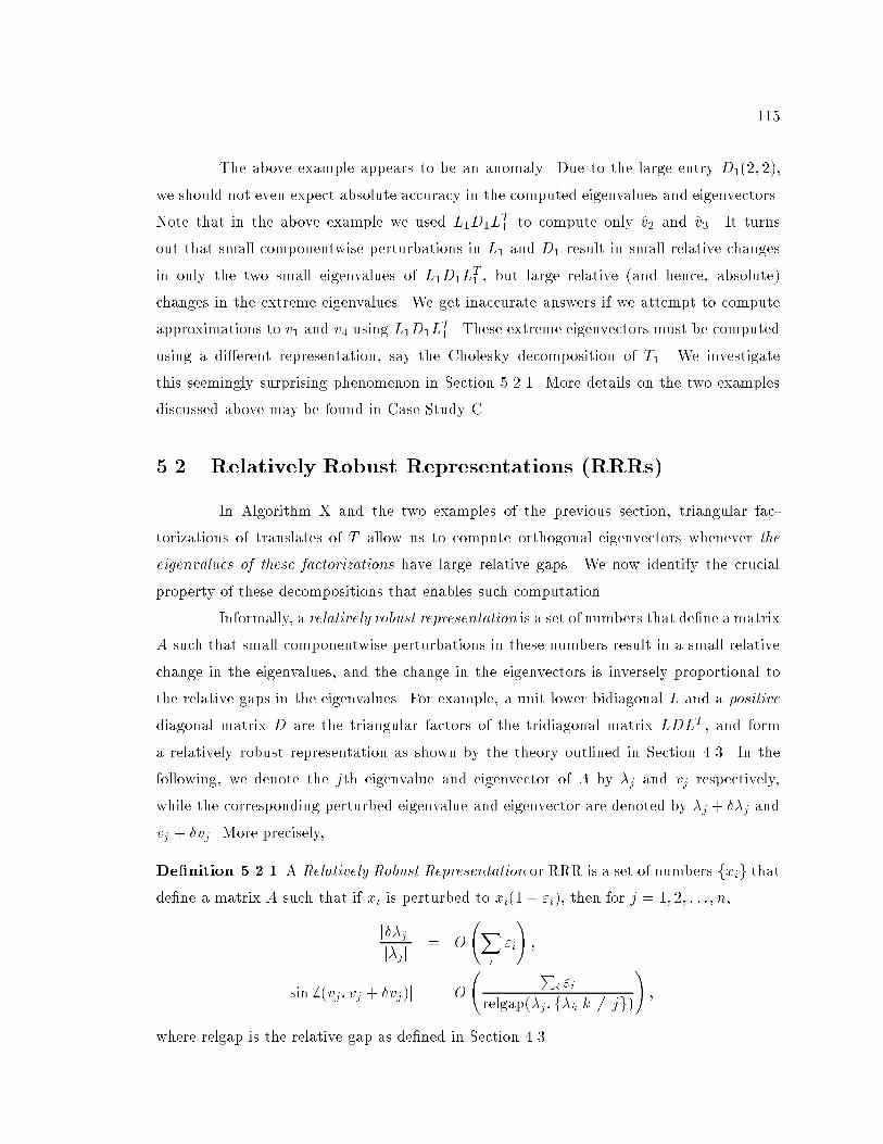
115
The above example appears to be an anomaly. Due to the large entry D1(2; 2),
we should not even expect absolute accuracy in the computed eigenvalues and eigenvectors.
Note that in the above example we used L1D1LT1 to compute only v2 and v3. It turns
out that small componentwise perturbations in L1 and D1 result in small relative changes
in only the two small eigenvalues of L1D1LT1 , but large relative (and hence, absolute)
changes in the extreme eigenvalues. We get inaccurate answers if we attempt to compute
approximations to v1 and v4 using L1D1LT1 . These extreme eigenvectors must be computed
using a di�erent representation, say the Cholesky decomposition of T1. We investigate
this seemingly surprising phenomenon in Section 5.2.1. More details on the two examples
discussed above may be found in Case Study C.
5.2 Relatively Robust Representations (RRRs)
In Algorithm X and the two examples of the previous section, triangular fac-
torizations of translates of T allow us to compute orthogonal eigenvectors whenever the
eigenvalues of these factorizations have large relative gaps. We now identify the crucial
property of these decompositions that enables such computation.
Informally, a relatively robust representation is a set of numbers that de�ne a matrix
A such that small componentwise perturbations in these numbers result in a small relative
change in the eigenvalues, and the change in the eigenvectors is inversely proportional to
the relative gaps in the eigenvalues. For example, a unit lower bidiagonal L and a positive
diagonal matrix D are the triangular factors of the tridiagonal matrix LDLT , and form
a relatively robust representation as shown by the theory outlined in Section 4.3. In the
following, we denote the jth eigenvalue and eigenvector of A by �j and vj respectively,
while the corresponding perturbed eigenvalue and eigenvector are denoted by �j + ��j and
vj + �vj . More precisely,
De�nition 5.2.1 A Relatively Robust Representation or RRR is a set of numbers fxig thatde�ne a matrix A such that if xi is perturbed to xi(1 + "i), then for j = 1; 2; : : : ; n,
j��jjj�jj
= O
Xi
"i
!;
j sin 6 (vj ; vj + �vj)j = O
Pi "i
relgap(�j; f�kjk 6= jg)
!;
where relgap is the relative gap as de�ned in Section 4.3.
116
Typically, the RRRs we consider will be triangular factors L and D of the shifted
matrix T � �I . We will frequently refer to such a factorization as a representation of T
(based) at the shift �. Also, for the sake of brevity, we will often refer to the underlying
matrix LDLT as the RRR (instead of the individual factors L and D). Sometimes a
representation may determine only a few but not all its eigenvalues to high relative accuracy.
For example, a representation may only determine the eigenvalues �j ; �j+1; : : : ; �k to high
relative accuracy. In such a case, we say that we have a partial RRR and denote it by
RRR(j; j + 1; : : : ; k). In the next section, we will show that the representation of T0 at the
shift 1 is an RRR while that of T1 at 1 is a partial RRR(2; 3), where T0 and T1 are the
matrices of Examples 5.1.1 and 5.1.2 respectively.
5.2.1 Relative Condition Numbers
We now �nd a criterion to judge if the factors L and D form an RRR. Instead
of dealing with LDLT we switch to a Cholesky-like decomposition for the purpose of our
analysis,
LDLT = ~L~LT ;
where = sign(D) is a matrix with �1 entries and explicitly captures the \inde�niteness"
of the matrix, and ~L is lower triangular. Note that is the identity matrix when LDLT is
positive de�nite. We made a similar switch in Chapter 5 where we analyzed the perturbation
properties of the Cholesky factor while performing our computations with LDLT . The
relationship between these alternate representations is easy to see and is given by
~L = L jDj1=2:
By Theorem 4.4.1, both these representations are similar in terms of their behavior under
small relative perturbations.
Thus we consider the factorization
T = ~L~LT : (5.2.4)
As shown in Section 4.3, if we make small componentwise perturbations in ~L, the perturbed
bidiagonal may be represented asD1~LD2 whereD1 andD2 are diagonal matrices close to the
identity matrix. We are interested in answering the following question. Are the eigenvalues
of the perturbed matrix
T + �T = D1~LD2D
T2~LTDT
1
117
relatively close to the eigenvalues of ~L~LT and if so, when? Note that the answer is always
in the a�rmative when = I , irrespective of the individual entries in ~L.
By Eisenstat and Ipsen's Theorem 2.1 in [49], the eigenvalues of DT1 AD1 are small
relative perturbations of the eigenvalues of A if kD1k � 1. By applying their result to our
case, we get
�j [~LD2DT2~LT ]
kD1k2� �j[T + �T ] � �j[~LD2D
T2~LT ] � kD1k2; (5.2.5)
where �j [A] denotes the jth eigenvalue of A.
We now write D2 as I + �2 where k�2k = O("). In proving the following result,
we use the fact that an eigenvalue of a matrix is a continuous function of its entries.
Theorem 5.2.1 Let � = �j be a simple eigenvalue of ~L~LT with eigenvector v = vj . Let
�+ �� be the corresponding eigenvector of ~L(I +�2)(I +�T2 )~LT . Then
�� = vT ~L(�2+�T2 )~LTv + O(k�2k2 � k~LTvk2); (5.2.6)
or
j��jj�j � jvT ~L~LT vj
jvT ~L~LTvj � 2k�2k+ O
jvT ~L~LT vjjvT ~L~LTvj � k�2k2
!: (5.2.7)
Proof. By continuity of the eigenvalues, we can write
�~L(I + �2)(I +�T
2 )~LT�(v + �v) = (�+ ��)(v + �v):
Expanding the terms, we get
(~L�2~LT + ~L�2
~LT + ~L�2�2~LT ) � v + ~L~LT � �v+
(~L�2~LT + ~L�2
~LT + ~L�2�2~LT ) � �v = ��v + �� � v + �� � �v:
Premultiplying both sides by vT ,
vT ~L�2~LTv + vT ~L�2
~LTv + �vT�v +O(kLTvk2 � k�2k2) = �vT�v + ��;
and by canceling the common term on both sides, we obtain (5.2.6). Dividing both sides
by the eigenvalue � and taking norms yields the result (5.2.7). tuWe call the ratio of the Rayleigh Quotients given in (5.2.7) as the relative condition
number of �j , and denote it by �rel, i.e.,
�rel(�j) =jvTj ~L~LTvj jjvTj ~L~LTvj j
: (5.2.8)
118
By combining (5.2.5) and (5.2.7) and using the above notation, we get
f1� 2 kI �D2k � �rel(�j[T ])g �j [T ]
kD1k2� �j [T + �T ]
� �j [T ] kD1k2 f1 + 2 kI �D2k � �rel(�j[T ])g ; (5.2.9)
which is correct to �rst-order terms.
We draw the reader's attention to the following facts :
1. Unlike the case of = I where all eigenvalues are relatively robust (see Section 4.3),
here a condition number measures the relative robustness of an eigenvalue.
2. The relative condition number �rel is di�erent for each eigenvalue. Thus some eigen-
values may be determined to high relative accuracy whereas others may not be. See
Example 5.2.2 for such an example.
3. A uniform bound for �rel is k~Lk � k~L�1k, and this bound holds for all eigenvalues
(see (5.2.13) below). However this bound can be a severe over-estimate as is shown
by the examples given later in Section 5.2.2.
4. Note that we did not constrain ~L to a bidiagonal form in deriving (5.2.9). However,
relative perturbations in the individual entries of a dense matrix ~L cannot be ex-
pressed as D1~LD2. There is only a restricted class of matrices whose componentwise
perturbations can be written in the form D1~LD2. Matrices that belong to this class
are completely characterized by the sparsity pattern of their non-zeros and have been
called the set of biacyclic matrices, a term coined by Demmel and Gragg in [33]. Be-
sides bidiagonal matrices, the twisted factors introduced in Section 3.1 and triangular
factors of arrowhead matrices (see [73, p.175]) belong to this class of matrices. Thus
the theory developed in this section is applicable not only to a bidiagonal matrix but
also to any biacyclic matrix.
By de�ning the vector
fjdef=
~LT vjqj�j j
; (5.2.10)
the relative condition number de�ned in (5.2.8) may be simply written as a norm,
�rel(�j) = fTj fj = kfjk2: (5.2.11)
119
Note that the following relationships hold,
~LTvj = fj
qj�j j; ~Lfj = vjsign(�j)
qj�jj;
and fTj fj = sign(�j); vTj vj = 1;
and so we call fj , the jth right -singular vector of ~L. Since ~L~LTvj = �jvj , and by (5.2.10),
fj may alternately be expressed as
fj = sign(�j)qj�jj � ~L�1vj : (5.2.12)
(5.2.10) and (5.2.12) suggest a bound for fTj fj ,
�rel(�j) = fTj fj � cond(~L) = k~Lk � k~L�1k; 8j: (5.2.13)
However the above bound is rather pessimistic since we want to compute the small eigen-
values of ~L~LT to high relative accuracy when the matrix is nearly singular, i.e., ~L is
ill-conditioned.
In [116], Parlett also arrived at such condition numbers for a bidiagonal ~L but by
using calculus.
Theorem 5.2.2 (Parlett [116, Thm. 2]) Let ~L be a bidiagonal matrix as in (4.3.3), with
ak 6= 0, bk 6= 0 and let = diag(!1; : : : ; !n) with !k = �1. Let (�,v) denote a particular
eigenpair of ~L~LT and let f be as de�ned in (5.2.10). Then by writing � = sign(�)�2, since
� 6= 0,
(a)@�
@ak� ak�
=kX
i=1
v(i)2� sign(�)k�1Xj=1
!jf(j)2 = sign(�)
nXm=k
!mf(m)2 �nX
l=k+1
v(l)2;
(b)@�
@bk� bk�
= sign(�)kX
i=1
!ip(i)2 �
kXj=1
v(j)2 =nX
m=k+1
v(m)2 � sign(�)nX
l=k+1
!lp(l)2:
For more work of a similar avor, see [34].
5.2.2 Examples
We now examine relative condition numbers of some factorizations
T � �I = ~L~LT ;
where T is tridiagonal and ~L is lower bidiagonal. In particular, we show that
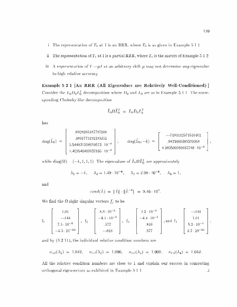
120
i. The representation of T0 at 1 is an RRR, where T0 is as given in Example 5.1.1.
ii. The representation of T1 at 1 is a partial RRR, where T1 is the matrix of Example 5.1.2.
iii. A representation of T � �I at an arbitrary shift � may not determine any eigenvalue
to high relative accuracy.
Example 5.2.1 [An RRR (All Eigenvalues are Relatively Well-Conditioned).]
Consider the L0D0LT0 decomposition where D0 and L0 are as in Example 5.1.1. The corre-
sponding Cholesky-like decomposition
~L0~LT0 = L0D0L
T0
has
diag(~L0) =
2666664
:6928203187797266
:3891773192193351
5:544821298610673 � 10�4
1:409546469637835 � 10�4
3777775 ; diag(~L0;�1) =
2664
�:7494442574516461
:9435080382529064
4:983500289685748 � 10�5
3775 ;
while diag() = (�1; 1; 1; 1). The eigenvalues of ~L0~LT0 are approximately
�1 = �1; �2 = 1:49 � 10�8; �3 = 2:98 � 10�8; �4 = 1;
and
cond(~L) = k~Lk � k~L�1k = 9:46 � 103:
We �nd the -right singular vectors fj to be
f1 =
2666664
1:01
�:144
7:5 � 10�5
�5:3 � 10�13
3777775 ; f2 =
2666664
8:8 � 10�5
�3:1 � 10�4
:577
�:816
3777775 ; f3 =
2666664
1:2 � 10�4
�4:4 � 10�4
:816
:577
3777775 ; and f4 =
2666664
�:144
1:01
5:2 � 10�4
3:7 � 10�12
3777775 :
and by (5.2.11), the individual relative condition numbers are
�rel(�1) = 1:042; �rel(�2) = 1:000; �rel(�3) = 1:000; �rel(�4) = 1:042:
All the relative condition numbers are close to 1 and explain our success in computing
orthogonal eigenvectors as exhibited in Example 5.1.1. tu
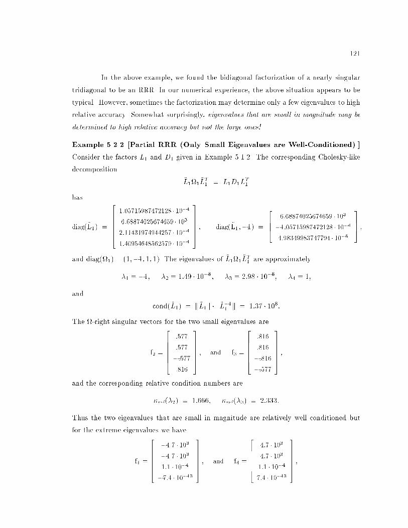
121
In the above example, we found the bidiagonal factorization of a nearly singular
tridiagonal to be an RRR. In our numerical experience, the above situation appears to be
typical. However, sometimes the factorization may determine only a few eigenvalues to high
relative accuracy. Somewhat surprisingly, eigenvalues that are small in magnitude may be
determined to high relative accuracy but not the large ones!
Example 5.2.2 [Partial RRR (Only Small Eigenvalues are Well-Conditioned).]
Consider the factors L1 and D1 given in Example 5.1.2. The corresponding Cholesky-like
decomposition
~L11~LT1 = L1D1L
T1
has
diag(~L1) =
2666664
1:05715987472128 � 10�4
6:68874025674659 � 103
2:11431974944257 � 10�4
1:40954648562579 � 10�4
3777775 ; diag(~L1;�1) =
2664
6:68874025674659 � 103
�1:05715987472128 � 10�4
4:98349983747794 � 10�5
3775 ;
and diag(1) = (1;�1; 1; 1). The eigenvalues of ~L11~LT1 are approximately
�1 = �1; �2 = 1:49 � 10�8; �3 = 2:98 � 10�8; �4 = 1;
and
cond(~L1) = k~L1k � k~L�11 k = 1:37 � 108:
The -right singular vectors for the two small eigenvalues are
f2 =
2666664
:577
:577
�:577
:816
3777775 ; and f3 =
2666664
:816
:816
�:816
�:577
3777775 ;
and the corresponding relative condition numbers are
�rel(�2) = 1:666; �rel(�3) = 2:333:
Thus the two eigenvalues that are small in magnitude are relatively well conditioned but
for the extreme eigenvalues we have
f1 =
2666664
�4:7 � 103
�4:7 � 103
1:1 � 10�4
�7:4 � 10�13
3777775 ; and f4 =
2666664
4:7 � 103
4:7 � 103
1:1 � 10�4
7:4 � 10�13
3777775 ;
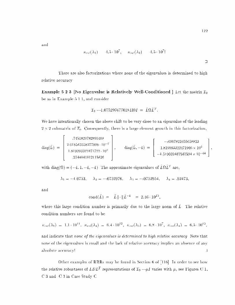
122
and
�rel(�1) = 4:5 � 107; �rel(�4) = 4:5 � 107!
tu
There are also factorizations where none of the eigenvalues is determined to high
relative accuracy.
Example 5.2.3 [No Eigenvalue is Relatively Well-Conditioned.] Let the matrix T0
be as in Example 5.1.1, and consider
T0 � 1:075297677018139I = ~L~LT :
We have intentionally chosen the above shift to be very close to an eigenvalue of the leading
2� 2 submatrix of T0. Consequently, there is a large element growth in this factorization,
diag(~L) =
2666664
:7451829782893468
2:018543658277998 � 10�7
1:819093322471722 � 106
:2744041812115826
3777775 ; diag(~L;�1) =
2664
�:6967821655658823
1:819093322471946� 106
�1:519032487587594� 10�14
3775 ;
with diag() = (�1; 1;�1;�1). The approximate eigenvalues of ~L~LT are,
�1 = �1:0753; �2 = �:0752976; �3 = �:0752954; �4 = :92473;
and
cond(~L) = k~Lk � k~L�1k = 2:46 � 1013;
where this large condition number is primarily due to the large norm of ~L. The relative
condition numbers are found to be
�rel(�1) = 1:1 � 1011; �rel(�2) = 6:4 � 1012; �rel(�3) = 6:8 � 107; �rel(�4) = 6:5 � 1012;
and indicate that none of the eigenvalues is determined to high relative accuracy. Note that
none of the eigenvalues is small and the lack of relative accuracy implies an absence of any
absolute accuracy! tu
Other examples of RRRs may be found in Section 6 of [116]. In order to see how
the relative robustness of LDLT representations of T0 � �I varies with �, see Figures C.1,
C.3 and C.3 in Case Study C.
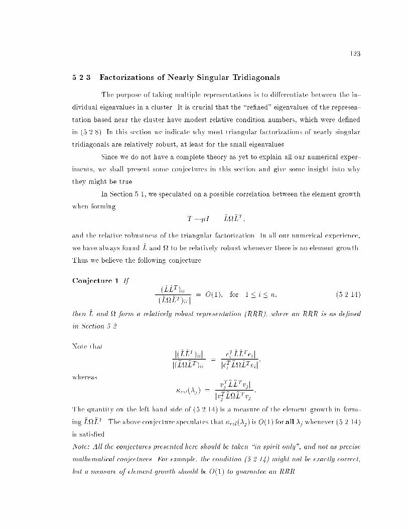
123
5.2.3 Factorizations of Nearly Singular Tridiagonals
The purpose of taking multiple representations is to di�erentiate between the in-
dividual eigenvalues in a cluster. It is crucial that the \re�ned" eigenvalues of the represen-
tation based near the cluster have modest relative condition numbers, which were de�ned
in (5.2.8). In this section we indicate why most triangular factorizations of nearly singular
tridiagonals are relatively robust, at least for the small eigenvalues.
Since we do not have a complete theory as yet to explain all our numerical exper-
iments, we shall present some conjectures in this section and give some insight into why
they might be true.
In Section 5.1, we speculated on a possible correlation between the element growth
when forming
T � �I = ~L~LT ;
and the relative robustness of the triangular factorization. In all our numerical experience,
we have always found ~L and to be relatively robust whenever there is no element growth.
Thus we believe the following conjecture.
Conjecture 1 If
j (~L~LT )ii jj (~L~LT )ii j
= O(1); for 1 � i � n; (5.2.14)
then ~L and form a relatively robust representation (RRR), where an RRR is as de�ned
in Section 5.2.
Note thatj(~L~LT )iijj(~L~LT )iij
=jeTi ~L~LTeijjeTi ~L~LTeij
;
whereas
�rel(�j) =jvTj ~L~LTvj jjvTj ~L~LTvj j
:
The quantity on the left hand side of (5.2.14) is a measure of the element growth in form-
ing ~L~LT . The above conjecture speculates that �rel(�j) is O(1) for all �j whenever (5.2.14)
is satis�ed.
Note: All the conjectures presented here should be taken \in spirit only", and not as precise
mathematical conjectures. For example, the condition (5.2.14) might not be exactly correct,
but a measure of element growth should be O(1) to guarantee an RRR.
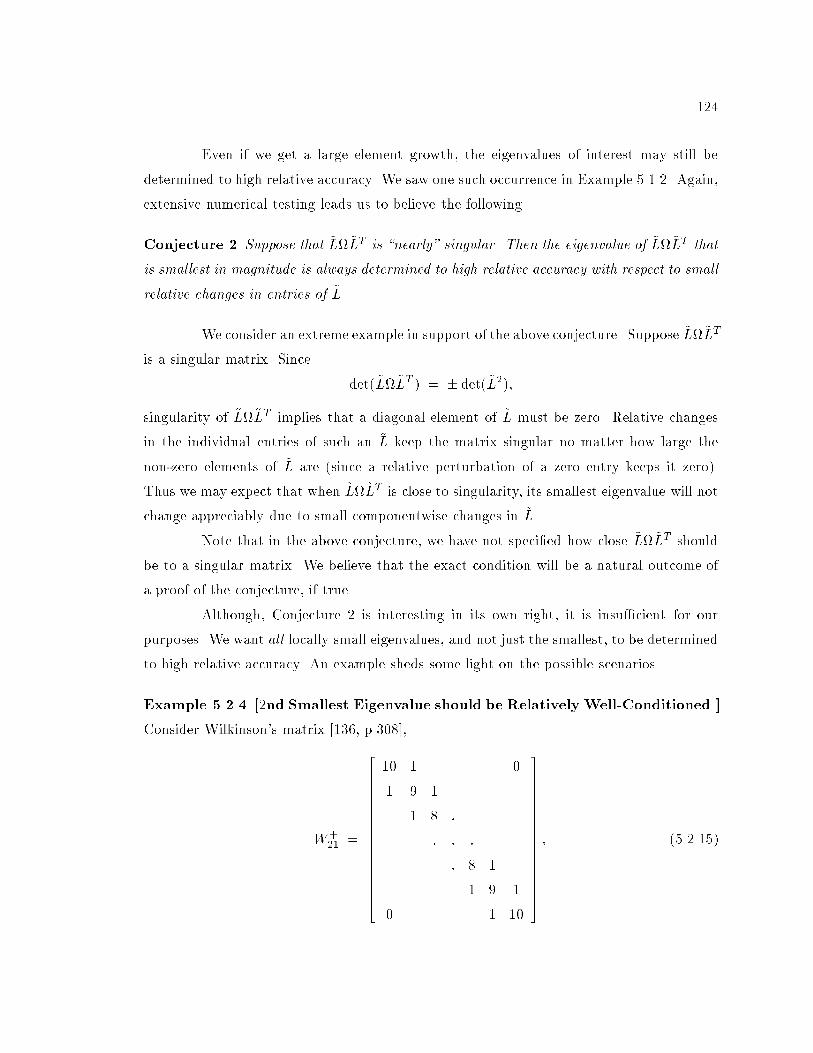
124
Even if we get a large element growth, the eigenvalues of interest may still be
determined to high relative accuracy. We saw one such occurrence in Example 5.1.2. Again,
extensive numerical testing leads us to believe the following.
Conjecture 2 Suppose that ~L~LT is \nearly" singular. Then the eigenvalue of ~L~LT that
is smallest in magnitude is always determined to high relative accuracy with respect to small
relative changes in entries of ~L.
We consider an extreme example in support of the above conjecture. Suppose ~L~LT
is a singular matrix. Since
det(~L~LT ) = � det(~L2);
singularity of ~L~LT implies that a diagonal element of ~L must be zero. Relative changes
in the individual entries of such an ~L keep the matrix singular no matter how large the
non-zero elements of ~L are (since a relative perturbation of a zero entry keeps it zero).
Thus we may expect that when ~L~LT is close to singularity, its smallest eigenvalue will not
change appreciably due to small componentwise changes in ~L.
Note that in the above conjecture, we have not speci�ed how close ~L~LT should
be to a singular matrix. We believe that the exact condition will be a natural outcome of
a proof of the conjecture, if true.
Although, Conjecture 2 is interesting in its own right, it is insu�cient for our
purposes. We want all locally small eigenvalues, and not just the smallest, to be determined
to high relative accuracy. An example sheds some light on the possible scenarios.
Example 5.2.4 [2nd Smallest Eigenvalue should be Relatively Well-Conditioned.]
Consider Wilkinson's matrix [136, p.308],
W+21 =
26666666666666664
10 1 0
1 9 1
1 8 :
: : :
: 8 1
1 9 1
0 1 10
37777777777777775
; (5.2.15)
125
which has pairs of eigenvalues that are close to varying degrees. For example, the eigenvalues
�14 = 7:003951798616376;
�15 = 7:003952209528675;
agree in 6 leading digits. We might try and form either
W+21 � �14I = L1D1L
T1 ; (5.2.16)
or
W+21 � �15I = L2D2L
T2 (5.2.17)
in order to compute orthogonal approximations to v14 and v15. We encounter a large element
growth when forming (5.2.16) but not in (5.2.17). Consistent with Conjectures 1 and 2,
we �nd L2D2LT2 to be an RRR whereas L1D1L
T1 only determines its smallest eigenvalue to
high relative accuracy. In particular,
�rel(�14[L1D1LT1 ]) = 2:246; �rel(�15[L1D1L
T1 ]) = 7:59� 108;
while
�rel(�14[L2D2LT2 ]) = 1:0; �rel(�15[L2D2L
T2 ]) = 1:0:
Thus L1D1LT1 is inadequate for our purposes whereas L2D2L
T2 enables us to compute v14
and v15 that are numerically orthogonal. tu
Finally, as in the above example, we believe we can always �nd a partial RRR
based at one of the eigenvalues in the cluster.
Conjecture 3 Suppose T is a tridiagonal matrix and �j ; �j+1; : : : ; �j+m�1 are approxima-
tions to m \close" eigenvalues of T , that agree in almost all their digits. Then at least one
of the factorizations
T � �sI = LsDsLTs ; j � s < j +m;
is a partial RRR(j; j+1; : : : ; j+m�1), i.e., LsDsLTs determines its locally small eigenvalues
to high relative accuracy.
The relative robustness of factorizations of nearly singular tridiagonals is consistent
with our earlier Conjecture 1. This is because we do not get any element growth in the
generic case when forming
T � �I = LDLT ;
126
where � is close to an eigenvalue of T .
Conjecture 3 is exactly what we need to achieve our goal of computing orthog-
onal eigenvectors. Furthermore, it would be even more e�cient if we could easily �nd the
particular �s in Conjecture 3 that leads to a relatively robust representation.
We leave it for future studies to provide further numerical evidence and theory to
prove or disprove the validity of the conjectures made in this section. From now on, we will
assume that Conjecture 3 is true so that we can �nd the desired RRRs.
5.2.4 Other RRRs
Until now, we have only considered computing a triangular decomposition, LDLT
or ~L~LT , as an RRR. However, we could also consider the twisted factorizations introduced
in Section 3.1 as RRRs. Indeed, since the set of n possible twisted factorizations
T � �I = N (k)�N (k)T ; 1 � k � n;
includes the LDLT decomposition, it may be easier to form such RRRs. Besides, it is
conceivable that a twisted factorization may be qualitatively better than a triangular de-
composition in terms of its relative perturbation properties. We believe that all conjectures
of the previous section also hold for twisted factorizations, and not only for triangular
factorizations.
5.3 Orthogonality using Multiple Representations
The examples of the previous section indicate that eigenvectors computed using a
single RRR turn out to be numerically orthogonal. If relative gaps are small, we form an
RRR near the cluster to get locally small eigenvalues that have large relative gaps. Some-
times, as in Example 5.1.2, we can only obtain a partial RRR the use of which guarantees
orthogonality of a limited set of eigenvector approximations. In such a case, the remaining
eigenvectors need to be computed using a di�erent RRR. In this section, we explain why the
approximations computed from one RRR are numerically orthogonal to the approximations
computed using another RRR. An added bene�t of the representation trees that we will
introduce for our exposition is that they summarize the computations involved and help us
in identifying computationally e�cient strategies.
127
5.3.1 Representation Trees
In Section 4.5, we provided a detailed proof of orthogonality of the eigenvectors
computed by Algorithm X using the LDLT decomposition of a positive de�nite tridiagonal
matrix when the eigenvalues have large relative gaps. This proof can easily be generalized
to the case when any �xed RRR is used for the computation. Similarly we can furnish
a detailed proof of orthogonality when di�erent RRRs are used for computing di�erent
eigenvectors. However, to avoid being drowned in detail, we choose an alternate approach.
We now introduce representation trees that informally indicate why vectors computed using
one RRR are orthogonal to those computed from another RRR. A formal treatment and
greater level of detail as in Corollary 4.5.4 can also be reproduced by mimicking its proof.
We remind the reader of our indexing convention for eigenvalues, by which
�1 � �2 � � � � � �n:
A representation tree consists of nodes that are denoted by (R; I) where R stands
for an RRR and I is a subset of the index set f1; 2; : : : ; ng. Informally, each node denotes
an RRR that is used enroute to computing eigenvectors of the eigenvalues �i[R] indexed
by I , i.e., i 2 I (note that we have used R in two ways | to denote the RRR and also for
the underlying matrix de�ned by the RRR). A parent node (Rp; Ip) can have m children
(Rj; Ij), 1 � j � m, such that
[jIj = Ip:
Any pair of the child nodes (R1; I1); (R2; I2) must satisfy
I1 � Ip; I2 � Ip; I1 \ I2 = �; (5.3.18)
and relgap2(�i[Rp]; �j[Rp]) � 1=n; 8i 2 I1; j 2 I2; i 6= j; (5.3.19)
where relgap2 is as de�ned in Section 4.3. Nodes that have no children will be called leaf
nodes while all other nodes are called intermediate nodes. The index set associated with any
leaf node must be a singleton. Each edge connecting a parent node to a child node will be
labeled by a real number �. Informally, an edge denotes the action of forming an RRR by
applying a shift of � to the matrix denoted by the parent RRR. Additionally, the shifts used
to form the leaf representations must be very accurate approximations to the appropriate
eigenvalues of the leaf's parent RRR. The condition on the relative gaps given by (5.3.19)
ensures that di�erent RRRs are formed in order to compute eigenvectors when relative gaps
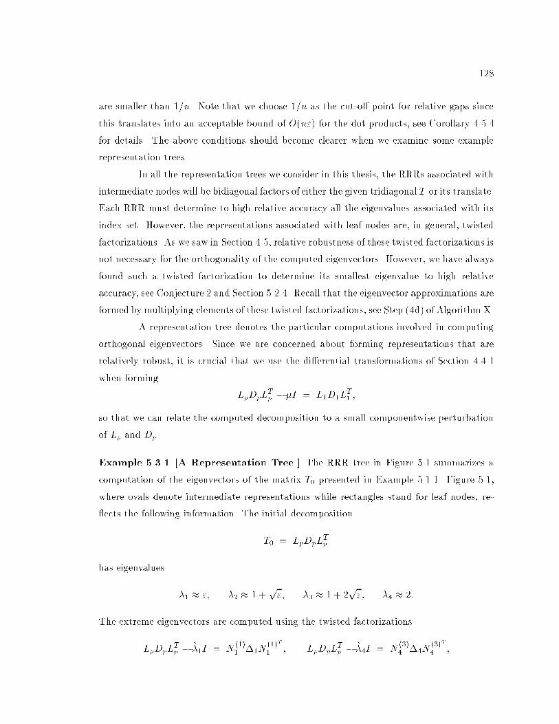
128
are smaller than 1=n. Note that we choose 1=n as the cut-o� point for relative gaps since
this translates into an acceptable bound of O(n") for the dot products, see Corollary 4.5.4
for details. The above conditions should become clearer when we examine some example
representation trees.
In all the representation trees we consider in this thesis, the RRRs associated with
intermediate nodes will be bidiagonal factors of either the given tridiagonal T or its translate.
Each RRR must determine to high relative accuracy all the eigenvalues associated with its
index set. However, the representations associated with leaf nodes are, in general, twisted
factorizations. As we saw in Section 4.5, relative robustness of these twisted factorizations is
not necessary for the orthogonality of the computed eigenvectors. However, we have always
found such a twisted factorization to determine its smallest eigenvalue to high relative
accuracy, see Conjecture 2 and Section 5.2.4. Recall that the eigenvector approximations are
formed by multiplying elements of these twisted factorizations, see Step (4d) of Algorithm X.
A representation tree denotes the particular computations involved in computing
orthogonal eigenvectors. Since we are concerned about forming representations that are
relatively robust, it is crucial that we use the di�erential transformations of Section 4.4.1
when forming
LpDpLTp � �I = L1D1L
T1 ;
so that we can relate the computed decomposition to a small componentwise perturbation
of Lp and Dp.
Example 5.3.1 [A Representation Tree.] The RRR tree in Figure 5.1 summarizes a
computation of the eigenvectors of the matrix T0 presented in Example 5.1.1. Figure 5.1,
where ovals denote intermediate representations while rectangles stand for leaf nodes, re-
ects the following information. The initial decomposition
T0 = LpDpLTp
has eigenvalues
�1 � "; �2 � 1 +p"; �3 � 1 + 2
p"; �4 � 2:
The extreme eigenvectors are computed using the twisted factorizations
LpDpLTp � �1I = N
(1)1 �1N
(1)T
1 ; LpDpLTp � �4I = N
(3)4 �4N
(3)T
4 ;
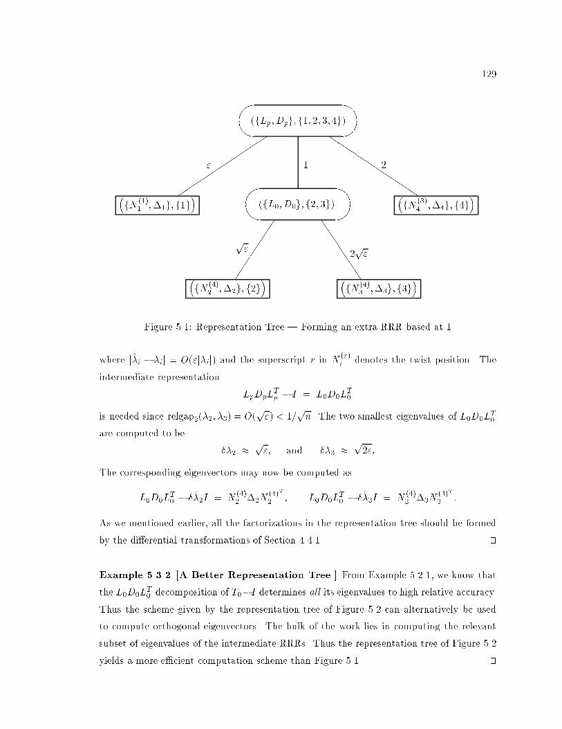
129
��
��(fLp; Dpg; f1; 2; 3; 4g)
�fN (1)
1 ;�1g; f1g� ��
��(fL0; D0g; f2; 3g)
�fN (3)
4 ;�4g; f4g�
�fN (4)
2 ;�2g; f2g� �
fN (4)3 ;�3g; f3g
�
��
��
��
��
��
QQQQQQQQQQ
J
J
J
J
J
JJ
" 1 2
p"
2p"
Figure 5.1: Representation Tree | Forming an extra RRR based at 1
where j�i � �ij = O("j�ij) and the superscript r in N(r)i denotes the twist position. The
intermediate representation
LpDpLTp � I = L0D0L
T0
is needed since relgap2(�2; �3) = O(p") < 1=
pn. The two smallest eigenvalues of L0D0L
T0
are computed to be
��2 �p"; and ��3 �
p2":
The corresponding eigenvectors may now be computed as
L0D0LT0 � ��2I = N
(4)2 �2N
(4)T
2 ; L0D0LT0 � ��3I = N
(4)3 �3N
(4)T
3 :
As we mentioned earlier, all the factorizations in the representation tree should be formed
by the di�erential transformations of Section 4.4.1. tu
Example 5.3.2 [A Better Representation Tree.] From Example 5.2.1, we know that
the L0D0LT0 decomposition of T0�I determines all its eigenvalues to high relative accuracy.
Thus the scheme given by the representation tree of Figure 5.2 can alternatively be used
to compute orthogonal eigenvectors. The bulk of the work lies in computing the relevant
subset of eigenvalues of the intermediate RRRs. Thus the representation tree of Figure 5.2
yields a more e�cient computation scheme than Figure 5.1. tu
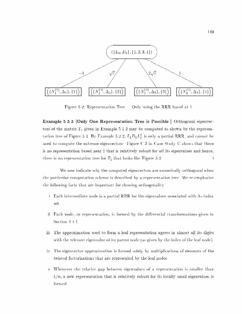
130
��
��(fL0; D0g; f1; 2; 3; 4g)
�fN (1)
1 ;�1g; f1g� �
fN (4)2 ;�2g; f2g
� �fN (4)
3 ;�3g; f3g� �
fN (3)4 ;�4g; f4g
�
��
��
��
��
��
��
���
J
J
J
J
J
J
JJ
HHHHHHHHHHHHHHH
�1 p" 2
p" 1
Figure 5.2: Representation Tree | Only using the RRR based at 1
Example 5.3.3 [Only One Representation Tree is Possible.] Orthogonal eigenvec-
tors of the matrix T1 given in Example 5.1.2 may be computed as shown by the represen-
tation tree of Figure 5.3. By Example 5.2.2, L1D1LT1 is only a partial RRR, and cannot be
used to compute the extreme eigenvectors. Figure C.3 in Case Study C shows that there
is no representation based near 1 that is relatively robust for all its eigenvalues and hence,
there is no representation tree for T1 that looks like Figure 5.2. tu
We now indicate why the computed eigenvectors are numerically orthogonal when
the particular computation scheme is described by a representation tree. We re-emphasize
the following facts that are important for showing orthogonality.
i. Each intermediate node is a partial RRR for the eigenvalues associated with its index
set.
ii. Each node, or representation, is formed by the di�erential transformations given in
Section 4.4.1.
iii. The approximation used to form a leaf representation agrees in almost all its digits
with the relevant eigenvalue of its parent node (as given by the index of the leaf node).
iv. The eigenvector approximation is formed solely by multiplications of elements of the
twisted factorizations that are represented by the leaf nodes.
v. Whenever the relative gap between eigenvalues of a representation is smaller than
1=n, a new representation that is relatively robust for its locally small eigenvalues is
formed.
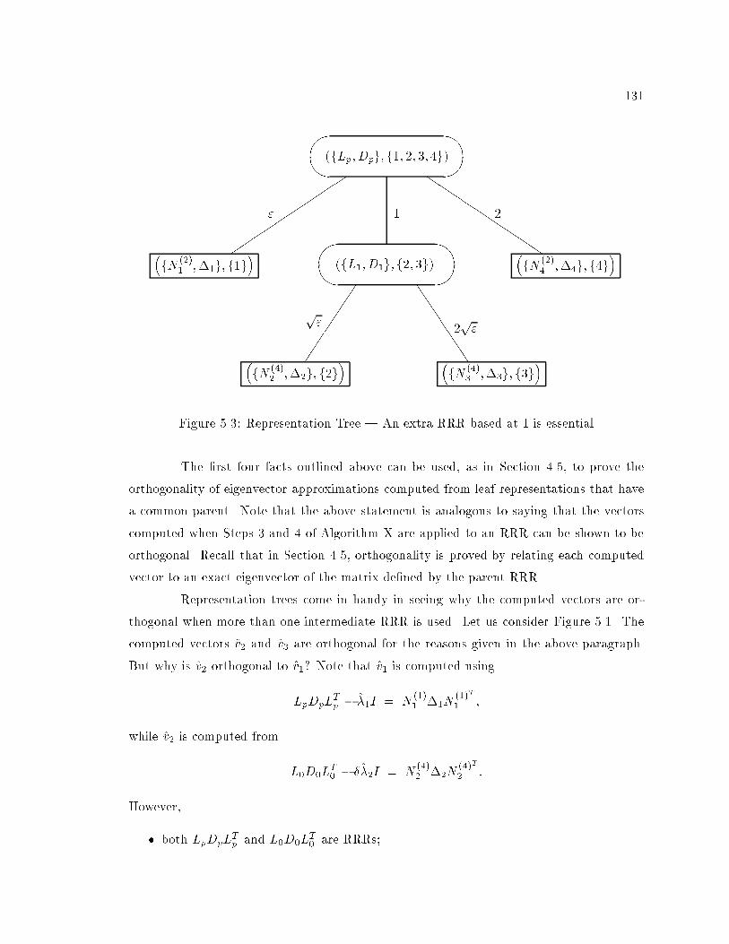
131
��
��(fLp; Dpg; f1; 2; 3; 4g)
�fN (2)
1 ;�1g; f1g� ��
��(fL1; D1g; f2; 3g)
�fN (2)
4 ;�4g; f4g�
�fN (4)
2 ;�2g; f2g� �
fN (4)3 ;�3g; f3g
�
��
��
��
��
��
QQQQQQQQQQ
J
J
J
J
J
JJ
" 1 2
p"
2p"
Figure 5.3: Representation Tree | An extra RRR based at 1 is essential
The �rst four facts outlined above can be used, as in Section 4.5, to prove the
orthogonality of eigenvector approximations computed from leaf representations that have
a common parent. Note that the above statement is analogous to saying that the vectors
computed when Steps 3 and 4 of Algorithm X are applied to an RRR can be shown to be
orthogonal. Recall that in Section 4.5, orthogonality is proved by relating each computed
vector to an exact eigenvector of the matrix de�ned by the parent RRR.
Representation trees come in handy in seeing why the computed vectors are or-
thogonal when more than one intermediate RRR is used. Let us consider Figure 5.1. The
computed vectors v2 and v3 are orthogonal for the reasons given in the above paragraph.
But why is v2 orthogonal to v1? Note that v1 is computed using
LpDpLTp � �1I = N
(1)1 �1N
(1)T
1 ;
while v2 is computed from
L0D0LT0 � ��2I = N
(4)2 �2N
(4)T
2 :
However,
� both LpDpLTp and L0D0L
T0 are RRRs;
132
� L0D0LT0 is a translate of LpDpL
Tp and is computed by the di�erential dstqds transfor-
mation of Section 4.4.1, and the roundo� error analysis given in Theorem 4.4.2 shows
that an exact relation exists between small componentwise perturbations of Lp, Dp
and L0, D0;
� the relative gap between �1 and �2 is large.
The vector v1 can directly be shown to be close to the �rst eigenvector of LpDpLTp ,
while v2 can be similarly related to the second eigenvector of LpDpLTp but via L0D0L
T0 . The
relative robustness of both these representations along with the above mentioned facts can
now be used to prove that v1 and v2 are orthogonal.
In general, any two eigenvectors computed from the twisted factorizations repre-
sented by the leaf nodes of a representation tree will be \good" approximations to distinct
eigenvectors of a common ancestor RRR. The properties satis�ed by a representation tree
now imply that these computed vectors must be orthogonal. Note that the detailed bounds
on the dot products of the computed vectors can get rather messy and would involve the
number of intermediate representations employed in computing an eigenvector. On the
other hand, representation trees provide a visual tool that makes it easy to see why the
computed vectors are nearly orthogonal. Besides this use, representation trees also allow
us to clearly see which computations are more e�cient.
5.4 Algorithm Y | orthogonality even when relative gaps
are small
We now present an algorithm that also handles small relative gaps but still per-
forms the computation in O(n2) time.
Algorithm Y [Computes orthogonal eigenvectors.]
1. Find � � kTk such that T + �I is positive (or negative) de�nite.
2. Compute T + �I = LpDpLTp .
3. Compute the eigenvalues, �j , of LpDpLTp to high relative accuracy by the dqds algo-
rithm [56].
4. Set l 1; m n.
133
5. Group the computed eigenvalues �l; : : : ; �m into the categories:
isolated. �j is isolated if
min(relgap2(�j; �j+1); relgap2(�j�1; �j)) � 1=n:
clustered. �j ; : : : ; �j+k�1 form a \cluster" of k eigenvalues if
relgap2(�i; �i+1) � 1=n; j � i < j + k � 1;
while relgap2(�j�1; �j) � 1=n; and relgap2(�j+k�1; �j+k) � 1=n:
6. For each isolated eigenvalue, � = �j , l � j � m, do the following
(a) Compute LpDpLTp � �I = L+D+L
T+ by the dstqds transform (Algorithm 4.4.3).
(b) Compute LpDpLTp � �I = U�D�UT� by the dqds transform (Algorithm 4.4.5).
(c) Compute k as in the top formula of (4.4.26). Pick r such that j rj = mink j kj.(d) Form the approximate eigenvector zj = z
(r)j by solving NrDrN
Tr zj = rer (see
Theorem 3.2.2):
zj(r) = 1;
zj(i) = �L+(i) � zj(i+ 1); i = r � 1; : : : ; 1;
zj(l+ 1) = �U�(l) � zj(l); l = r; : : : ; n� 1:
7. For each cluster �j ; : : : ; �j+k�1 do the following.
(a) Get a partial RRR(j; : : : ; j + k � 1) by forming the dstqds transformation
LpDpLTp � �sI = LsDsL
Ts ;
where j � s � j + k � 1.
(b) Compute the jth through (j + k � 1)th eigenvalues of LsDsLTs to high relative
accuracy and call them ��j; : : : ; ��j+k�1.
(c) Set l j, m i+ k � 1, �i ��i for j � i � j + k � 1, Lp Ls, Dp Ds,
and go to Step 5.
tuThe previous section indicates why the vectors computed by Algorithm Y are
numerically orthogonal. We now present detailed numerical results comparing a computer
implementation of Algorithm Y with existing software routines.
134
Chapter 6
A Computer Implementation
In this chapter, we give detailed timing and accuracy results of a computer imple-
mentation of Algorithm Y, whose pseudocode was given in Section 5.4. The only uncertainty
in implementing this algorithm is in its Step (7a), where we need to choose a shift � near
a cluster in order to form the relatively robust representation
LpDpLTp � �I = LDLT : (6.0.1)
We brie y discuss our strategy in Section 6.1. Having found a suitable representation, we
need to �nd its locally small eigenvalues to high relative accuracy in Step (7b) of Algo-
rithm Y. In Section 6.2, we give an e�cient scheme to �nd these small eigenvalues to the
desired accuracy. Note that the earlier steps of Algorithm Y have been discussed in great
detail in Chapter 4.
Finally, in Section 6.4, we give detailed timing and accuracy results comparing our
computer implementation of Algorithm Y with existing LAPACK and EISPACK software.
Our test-bed contains a variety of tridiagonal matrices, some from quantum chemistry
applications, that highlight the sensitivity of earlier algorithms to di�erent distributions of
eigenvalues. The test matrices are discussed in Section 6.4.1.
We �nd that our implementation of Algorithm Y is uniformly faster than earlier
implementations of inverse iteration, while still being accurate. This speed is by virtue
of the O(n2) running time of Algorithm Y as opposed to the earlier algorithms that take
O(n3) time in general. We want to stress that the results presented in the chapter are
preliminary | we can envisage more algorithmic enhancements and a better use of the
memory hierachy and architectural design (such as multiple functional units in the CPU)
135
of modern computers to further speed up our computer implementation. Some of these
enhancements are brie y discussed in Section 6.5, and we hope to incorporate such code
improvements in the near future.
6.1 Forming an RRR
Two questions, that need to be resolved to get a computer implementation of
Step (7a) of Algorithm Y, were raised in Sections 5.2.1 and 5.2.3:
1. What shift � near a cluster should we choose so that the LDLT decomposition
of (6.0.1) is an RRR?
2. Given LDLT , how can we cheaply decide if it is an RRR?
As we saw earlier in Example 5.2.3, not every � in (6.0.1) leads to an RRR. We
do not have any a priori way of knowing whether an arbitrary choice of � would lead to
a desired RRR. Indeed, as Example 5.2.4 suggests, there may not be any alternative other
than actually forming LDLT at a judicious choice of � and then, a posteriori, checking
whether this decomposition forms an RRR. Since we want an e�cient procedure for the
latter purpose, we cannot a�ord to evaluate the relative condition numbers of Section 5.2.1.
Thus, answers to the two questions posed above are crucial to a correct implementation.
We made several conjectures in Section 5.2.3 that attempt to answer these ques-
tions. In our computer implementation, we have made the following decisions which re ect
our belief in these conjectures.
1. After identifying a cluster of eigenvalues �j ; �j+1; : : : ; �j+k�1, we restrict our search
for an RRR to a factorization based at one of these �'s, i.e., to
LpDpLTp � �sI = LsDsL
Ts ; j � s � j + k � 1: (6.1.2)
This is the strategy given in Step (7a) of Algorithm Y and is consistent with Conjec-
ture 3.
2. When trying to form the desired RRR in (6.1.2), we try � = �s in the order s =
j; j+ 1; : : : ; j+ k� 1. If we �nd the element growth, as de�ned in (5.1.2), at some �s
to be less than an acceptable tolerance, say 200, then we immediately accept LsDsLTs
as the desired RRR. By this strategy, we are often able to form an RRR in the �rst
136
attempt, i.e., based at the leftmost eigenvalue � = �j . This saves us the extra work
of forming all possible k factorizations of (6.1.2). Note that this approach re ects our
belief in Conjecture 1.
3. If all the above choices of � lead to element growths bigger than 200, as in Exam-
ple 5.2.2 (see also Case Study C), we choose the LsDsLTs decomposition that leads to
the least element growth as our partial RRR.
We want to emphasize that even though we cannot prove the correctness of the
above decisions as yet, our computer implementation gives accurate answers on all our tests.
We have tested our implementation on tridiagonal matrices that are quite varied in their
eigenvalue distributions. See Section 6.4.1 for details.
6.2 Computing the Locally Small Eigenvalues
Until now, we have not discussed ways of e�ciently computing the eigenvalues of
a relatively robust representation. All eigenvalues of the LDLT decomposition of a positive
de�nite matrix may be e�ciently found by the dqds algorithm, and this is the method
employed in Step 3 of Algorithm Y. In its present form, the dqds algorithm �nds the
eigenvalues in sequential order, from the smallest to the largest, and always operates on a
positive de�nite matrix. See [56] for more details. The main di�culty in trying to employ
the dqds algorithm to �nd the locally small eigenvalues of an RRR is that in most cases,
the RRR will be the factorization of an inde�nite matrix. It is not known, as yet, if the
dqds algorithm can be adapted to an inde�nite case and hence we need to �nd an alternate
method.
One means of �nding the locally small eigenvalues is the bisection algorithm, using
any of the di�erential transformations given in Section 4.4.1 as the inner loop. However,
since bisection is a rather slow method, it could become the dominant part of the computa-
tion. So we use a faster scheme which is a slight variant of the Rayleigh Quotient Iteration
(RQI). A traditional RQI method starts with some (well-chosen) vector q0 and progresses by
computing Rayleigh Quotients to get increasingly better approximations to an eigenvalue.
Algorithm 6.2.1 [Traditional RQI.]
1. Choose a vector q0 (kq0k = 1), and a scalar �0. Set i 0.
137
2. Solve (T � �iI)xi+1 = qi for xi+1.
3. Set qi+1 xi+1=kxi+1k, �i+1 qTi+1Tqi+1, i i+ 1, and repeat Step 2. tu
As shown in Corollary 3.2.1, a twisted factorization allows us to cheaply compute
the Rayleigh Quotient of the vector z where
(T � �I)z = rer ; z(r) = 1; (6.2.3)
and r is an element of the twisted factorization at twist position r. It is immediately seen
from (6.2.3) that
zT (T � �I)z
zT z=
r
zTz:
As discussed earlier, it is possible to choose r so that r is proportional to the distance
of � from an eigenvalue of T . The index r where j rj = mink j kj is one such choice, see
Section 3.1 for more details. Thus we get the following iteration scheme.
Algorithm 6.2.2 [RQI-Like (Computes an eigenvalue of LsDsLTs ).]
1. Choose a scalar �0. Set i 0.
2. Choose an index r as follows :
(a) Compute LsDsLTs ��iI = L+D+L
T+ by the dstqds transform (Algorithm 4.4.3).
(b) Compute LsDsLTs � �iI = U�D�UT
� by the dqds transform (Algorithm 4.4.5).
(c) Compute k as in the top formula of (4.4.26). Pick r such that j rj = mink j kj.
3. Solve (LsDsLTs � �iI)zi = rer as follows
zi(r) = 1;
zi(p) = �L+(p) � zi(p+ 1); p = r � 1; : : : ; 1;
zi(q + 1) = �U�(q) � zi(q); q = r; : : : ; n� 1:
4. Set �i = r=kzik2, i i+ 1. Repeat Step 2. tu
In the above RQI-like scheme, we obtain the Rayleigh Quotient as a by-product of
computing the vector zi. One iteration of the above algorithm is only 2-3 times as expensive
as one bisection step, but convergence is at least quadratic. Note that Step 3 given above
138
di�ers from traditional RQI in its choice of er as the right hand side of the linear system to
be solved.
As outlined in Step (7a) of Algorithm Y (see Section 5.4), the representation
LsDsLTs is a translate of the original matrix LpDpL
Tp , i.e.,
LpDpLTp � �I = LsDsL
Ts : (6.2.4)
If � is an eigenvalue of LpDpLTp , ��� is the corresponding eigenvalue of LsDsL
Ts if
the relation (6.2.4) holds exactly. However, we only know an approximate eigenvalue �, and
roundo� errors are inevitable in forming Ls and Ds. But, even though ��� is not an exact
eigenvalue of the computed LsDsLTs , it does give us a very good starting approximation.
As a result, �0 can be initialized to � � � in Step 1 of our RQI-like scheme. Of course, as
emphasized in Chapter 5, we need to compute each small eigenvalue of LsDsLTs to high
relative accuracy. Since we compute both forward and backward pivots, D+ and D�, we
can include the safeguards of bisection in our iteration.
6.3 An Enhancement using Submatrices
In this section, we brie y mention a novel idea that facilitates the computation
of orthogonal \eigenvectors" of eigenvalues that are very close to each other but are well-
separated from the rest of the spectrum.
Eigenvalues of a tridiagonal matrix can be equal only if an o�-diagonal element
is zero. In such a case, the tridiagonal matrix is a direct sum of smaller tridiagonals,
and orthogonal eigenvectors are trivially obtained from the eigenvectors of these disjoint
submatrices by padding them with zeros. However, as Wilkinson observed, eigenvalues can
be arbitrarily close without any o�-diagonal element being small [136]. It turns out that
even in such a case, a good orthogonal basis of the invariant subspace can be computed by
using suitable, possibly overlapping, submatrices. Thus we can use the following scheme:
Algorithm 6.3.1 [Computes orthogonal \eigenvectors" for tight clusters using
submatrices.]
1. For each of the \close" eigenvalues �j ; : : : ; �k (that are well-separated from the rest
of the spectrum), do the following:
(a) \Find" a submatrix T p:q with an isolated eigenvalue � which is \close" to the
cluster of eigenvalues.
139
(b) Compute the eigenvector of �, i.e., solve (T p:q � �I)s = 0 for s.
(c) Output the vector v as an eigenvector, where vp:q = s and the rest of v is padded
with zeroes. tu
For some of the theory underlying this scheme, the reader is referred to Parlett [112,
115]. Clearly, besides the existence of suitable submatrices, the crucial question is: how do
we choose the submatrices in Step (1a) of the above scheme. The computation of the
eigenvector of an isolated eigenvalue in Step (1b) is easily done by using the methods
discussed earlier.
We now have a more robust way of picking the appropriate submatrices than the
approaches outlined in [112, 115]. We have included this enhancement in our implemen-
tation of Algorithm Y and found it to work accurately in practice. Note that the above
algorithm is an alternate way of computing orthogonal eigenvectors without doing any ex-
plicit orthogonalization. The smaller the submatrix sizes in Step (1b) above, the less is the
work required to produce orthogonal eigenvectors.
It is beyond the scope of this thesis to discuss the above approach in greater detail.
The theory that justi�es this scheme is quite involved and intricate, and a cursory treatment
would not do it justice. We hope to present more details in the near future [43].
6.4 Numerical Results
In this section, we present a numerical comparison between Algorithm Y and four
other software routines for solving the symmetric tridiagonal eigenproblem that are included
in the EISPACK [128] and LAPACK [1] libraries. These are
1. LAPACK INVIT : The LAPACK implementation of bisection and inverse iteration [88,
84, 87] (subroutines DSTEBZ and DSTEIN);
2. EISPACK INVIT : The EISPACK implementation of inverse iteration after �nding
the eigenvalues by bisection [118] (subroutine DSTEBZ from LAPACK followed by
TINVIT from EISPACK);
3. LAPACK D&C : The LAPACK implementation of the divide and conquer method
that uses a rank-one tear to subdivide the problem [71, 124] (subroutine DSTEDC);
140
4. LAPACK QR : The LAPACK implementation of the QR algorithm that uses Wilkin-
son's shifts to compute both eigenvalues and eigenvectors [69] (subroutine DSTEQR).
6.4.1 Test Matrices
We have chosen many di�erent types of tridiagonals as our test matrices. They
di�er mainly in their eigenvalue distributions which highlight the sensitivity of the above
algorithms as discussed in Chapter 2. Some of our example tridiagonals come from quantum
chemistry applications. The �rst eleven among the following types of tridiagonal matrices
are obtained by Householder reduction of random dense symmetric matrices that have the
given eigenvalue distributions (see [36] for more on the generation of such matrices). The
matrix sizes for our tests range from 125-2000.
1) Uniform Distribution (" apart). n � 1 eigenvalues uniformly distributed from " to
(n� 1)", and the nth eigenvalue at 1, i.e.,
�i = i � "; i = 1; 2; : : : ; n� 1; and �n = 1:
These matrices are identical to the Type 1 matrices of Section 4.6.
2) Uniform Distribution (p" apart). One eigenvalue at ", n� 2 eigenvalues uniformly
distributed from 1 +p" to 1 + (n� 2)
p", and the last eigenvalue at 2, i.e.,
�1 = "; �i = 1 + (i� 1) � p"; i = 2; : : : ; n� 1; and �n = 2:
These are also identical to the Type 2 matrices of Section 4.6.
3) Uniform Distribution (" to 1). The eigenvalues are equi-spaced between " and 1,
i.e.,
�i = "+ (i� 1) � �; i = 1; 2; : : : ; n
where � = (1� ")=(n� 1).
4) Uniform Distribution (" to 1 with random signs). Identical to the above type of
matrices except that a random � sign is attached to the eigenvalues.
5) Geometric Distribution (" to 1). The eigenvalues are geometrically arranged be-
tween " and 1, i.e.,
�i = "(n�i)=(n�1); i = 1; 2; : : : ; n:
141
6) Geometric Distribution (" to 1 with random signs). Identical to the above type
except that a random � sign is attached to the eigenvalues.
7) Random. The eigenvalues come from a random, normal (0; 1) distribution.
8) Clustered at 1. �1 = ", and �2 � �3 � � � � � �n � 1.
9) Clustered at �1. Identical to the above type except that a random � sign is attached
to the eigenvalues.
10) Clustered at ". �1 � �2 � � � � � �n�1 � ", and �n = 1.
11) Clustered at �". Identical to the above type of matrices except that a random �sign is attached to the eigenvalues.
12) (1,2,1) Matrix. These are the Toeplitz tridiagonal matrices with 2's on the diagonals
and 1's as the o�-diagonal elements. An n�n version of such a matrix has eigenvalues
4 sin2[k�=2(n+ 1)], and for the values of n under consideration, these eigenvalues are
not too close.
Matrices of types 3 through 11 above are LAPACK test matrices and are used to
check the accuracy of all LAPACK software for the symmetric tridiagonal eigenproblem. In
addition, the following symmetric tridiagonal matrices arise in certain quantum chemistry
computations. For more details on these problems, the reader is referred to [10, 55].
13) Biphenyl. This positive de�nite matrix with n = 966 occurs in the modeling of
biphenyl using M�ller-Plesset theory. Most of its eigenvalues are quite small com-
pared to the norm. See Figure 6.1 for a plot of its eigenvalue distribution.
14) SiOSi6. Density functional theory methods for determining bulk properties for the
molecule SiOSi6 lead to this positive de�nite matrix with n = 1687. Most of the
eigenvalues are quite close to their neighbors and there is no obvious subdivision of
the spectrum into separate clusters. Figure 6.2 gives this distribution.
15) Zeolite ZSM-5. This 2053�2053matrix occurs in the application of the self-consistent�eld(SCF) Hartree-Fock method for solving a non-linear Schr�odinger problem. See
Figure 6.3 for the spectrum.
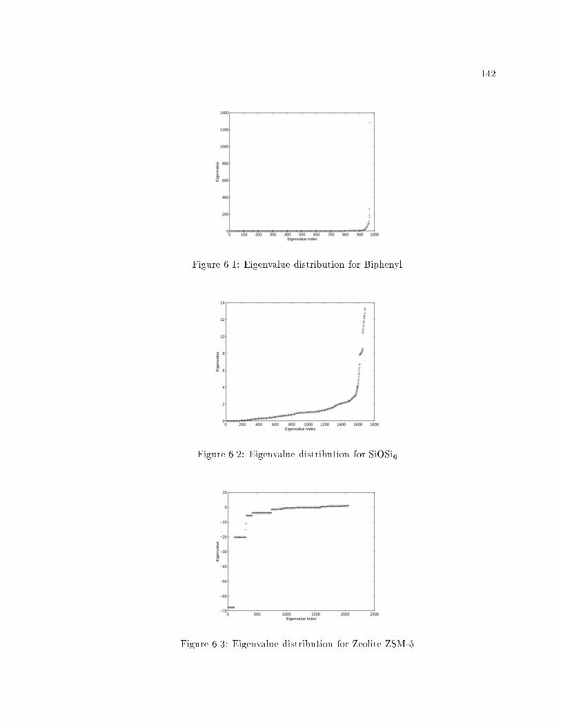
142
0 100 200 300 400 500 600 700 800 900 10000
200
400
600
800
1000
1200
1400
Eigenvalue Index
Eig
enva
lue
Figure 6.1: Eigenvalue distribution for Biphenyl
0 200 400 600 800 1000 1200 1400 1600 18000
2
4
6
8
10
12
14
Eigenvalue Index
Eig
enva
lue
Figure 6.2: Eigenvalue distribution for SiOSi6
0 500 1000 1500 2000 2500−70
−60
−50
−40
−30
−20
−10
0
10
Eigenvalue Index
Eig
enva
lue
Figure 6.3: Eigenvalue distribution for Zeolite ZSM-5
143
6.4.2 Timing and Accuracy Results
Tables 6.1 and 6.2 give a comparison of the times taken by the di�erent algorithms
to �nd all the eigenvalues and eigenvectors of symmetric tridiagonal matrices of the type
discussed above. All the numerical experiments presented in this section were conducted
on an IBM RS/6000-590 processor that has a peak rating of 266 MFlops. Fortran BLAS,
instead of those from the machine optimized ESSL library [82], were used in this preliminary
testing1. We hope to include the ESSL BLAS in our future comparisons. The rest of the
tables, Table 6.3 through 6.6, indicate the accuracy of the methods tested.
Our Algorithm Y may be thought of as an alternate way of doing inverse iteration.
Thus LAPACK INVIT and EISPACK INVIT are the two earlier methods that most closely
resemble Algorithm Y. Tables 6.1 and 6.2 show that Algorithm Y is always faster than both
these existing implementations. The di�erence in speed varies according to the eigenvalue
distribution | on matrices of order 2000, Algorithm Y is over 3500 times faster than
LAPACK INVIT when the eigenvalues are clustered around " while it is 4 times faster
when the eigenvalues are well-separated. These di�erent speedups highlight the sensitivity
of the various algorithms to the eigenvalue distribution. When eigenvalues are clustered,
EISPACK and LAPACK inverse iteration need O(n3) time, as is clear from Tables 6.1
and 6.2. On the other hand, they take O(n2) time when eigenvalues are isolated, see the
results for matrices of type 4 and type 7 in Table 6.1. We also draw the reader's attention to
the varying behavior on matrices with uniformly distributed eigenvalues (from " to 1), and
the (1; 2; 1) matrix. For small n, we see an O(n2) behavior but for larger n, both EISPACK
and LAPACK inverse iteration take O(n3) time. This discrepancy is due to the clustering
criterion which is independent of n | more speci�cally, reorthogonalization is done when
eigenvalues di�er by less than 10�3kTk. See Section 2.8.1 for more details. EISPACK's
implementation is always faster than LAPACK's but is generally, less accurate. In fact, the
latter was designed to improve the accuracy of EISPACK [87].
Algorithm Y is much less sensitive to the arrangement of eigenvalues | on matrices
of order 2000, the time taken by it ranges from about 30 seconds to about 60 seconds in
most cases. The two notable exceptions are the matrices where almost all eigenvalues are
clustered around " or �". It turns out that the eigenvectors of such matrices can be very
sparse | in fact, an identity matrix is a good approximation to an eigenvector matrix. By
1all code was compiled with the command line f77 -u -O, where the -O compiler option is identical to
the -O2 level of optimization
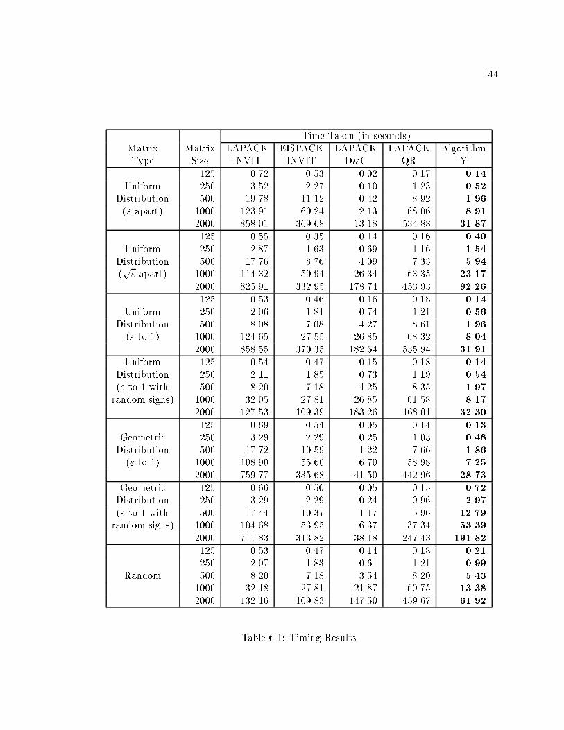
144
Time Taken (in seconds)
Matrix Matrix LAPACK EISPACK LAPACK LAPACK Algorithm
Type Size INVIT INVIT D&C QR Y
125 0.72 0.53 0.02 0.17 0.14
Uniform 250 3.52 2.27 0.10 1.23 0.52
Distribution 500 19.78 11.12 0.42 8.92 1.96
(" apart) 1000 123.91 60.24 2.13 68.06 8.91
2000 858.01 369.68 13.18 534.88 31.87
125 0.55 0.35 0.14 0.16 0.40
Uniform 250 2.87 1.63 0.69 1.16 1.54
Distribution 500 17.76 8.76 4.09 7.33 5.94
(p" apart) 1000 114.32 50.94 26.34 63.35 23.17
2000 825.91 332.95 178.74 453.93 92.26
125 0.53 0.46 0.16 0.18 0.14
Uniform 250 2.06 1.81 0.74 1.21 0.56
Distribution 500 8.08 7.08 4.27 8.61 1.96
(" to 1) 1000 124.65 27.55 26.85 68.32 8.04
2000 858.55 370.35 182.64 535.94 31.91
Uniform 125 0.54 0.47 0.15 0.18 0.14
Distribution 250 2.11 1.85 0.73 1.19 0.54
(" to 1 with 500 8.20 7.18 4.25 8.35 1.97
random signs) 1000 32.05 27.81 26.85 61.58 8.17
2000 127.53 109.39 183.26 468.01 32.30
125 0.69 0.54 0.05 0.14 0.13
Geometric 250 3.29 2.29 0.25 1.03 0.48
Distribution 500 17.72 10.59 1.22 7.66 1.86
(" to 1) 1000 108.90 55.60 6.70 58.98 7.25
2000 759.77 335.68 41.50 442.96 28.73
Geometric 125 0.66 0.50 0.05 0.15 0.72
Distribution 250 3.29 2.29 0.24 0.96 2.97
(" to 1 with 500 17.44 10.37 1.17 5.96 12.79
random signs) 1000 104.68 53.95 6.37 37.34 53.39
2000 711.83 313.82 38.18 247.43 191.82
125 0.53 0.47 0.14 0.18 0.21
250 2.07 1.83 0.61 1.21 0.99
Random 500 8.20 7.18 3.54 8.20 5.43
1000 32.18 27.81 21.87 60.75 13.38
2000 132.16 109.83 147.50 459.67 61.92
Table 6.1: Timing Results
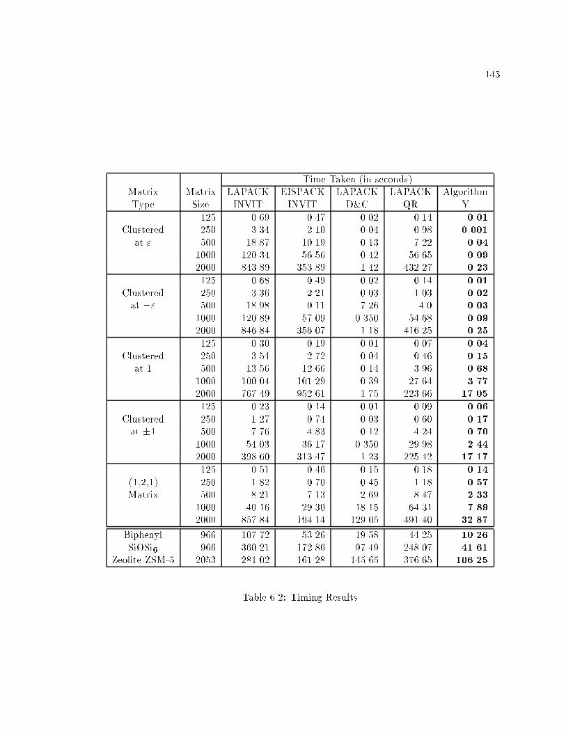
145
Time Taken (in seconds)
Matrix Matrix LAPACK EISPACK LAPACK LAPACK Algorithm
Type Size INVIT INVIT D&C QR Y
125 0.69 0.47 0.02 0.14 0.01
Clustered 250 3.34 2.10 0.04 0.98 0.001
at " 500 18.87 10.19 0.13 7.22 0.04
1000 120.34 56.56 0.42 56.65 0.09
2000 843.89 353.89 1.42 432.27 0.23
125 0.68 0.49 0.02 0.14 0.01
Clustered 250 3.36 2.21 0.03 1.03 0.02
at �" 500 18.98 0.11 7.26 4.0 0.03
1000 120.89 57.09 0.350 54.68 0.09
2000 846.84 356.07 1.18 416.25 0.25
125 0.30 0.19 0.01 0.07 0.04
Clustered 250 3.54 2.72 0.04 0.46 0.15
at 1 500 13.56 12.66 0.14 3.96 0.68
1000 100.04 101.29 0.39 27.64 3.77
2000 767.49 952.61 1.75 223.66 17.05
125 0.23 0.14 0.01 0.09 0.06
Clustered 250 1.27 0.74 0.03 0.60 0.17
at �1 500 7.76 4.83 0.12 4.24 0.70
1000 54.03 36.17 0.350 29.98 2.44
2000 398.60 313.47 1.23 225.42 17.17
125 0.51 0.46 0.15 0.18 0.14
(1,2,1) 250 1.82 0.70 0.45 1.18 0.57
Matrix 500 8.21 7.13 2.69 8.47 2.33
1000 40.16 29.30 18.15 64.31 7.89
2000 857.84 194.14 129.05 491.40 32.87
Biphenyl 966 107.72 53.26 19.58 44.25 10.26
SiOSi6 966 360.21 172.86 97.49 248.07 41.61
Zeolite ZSM-5 2053 281.02 161.28 145.65 376.65 106.25
Table 6.2: Timing Results
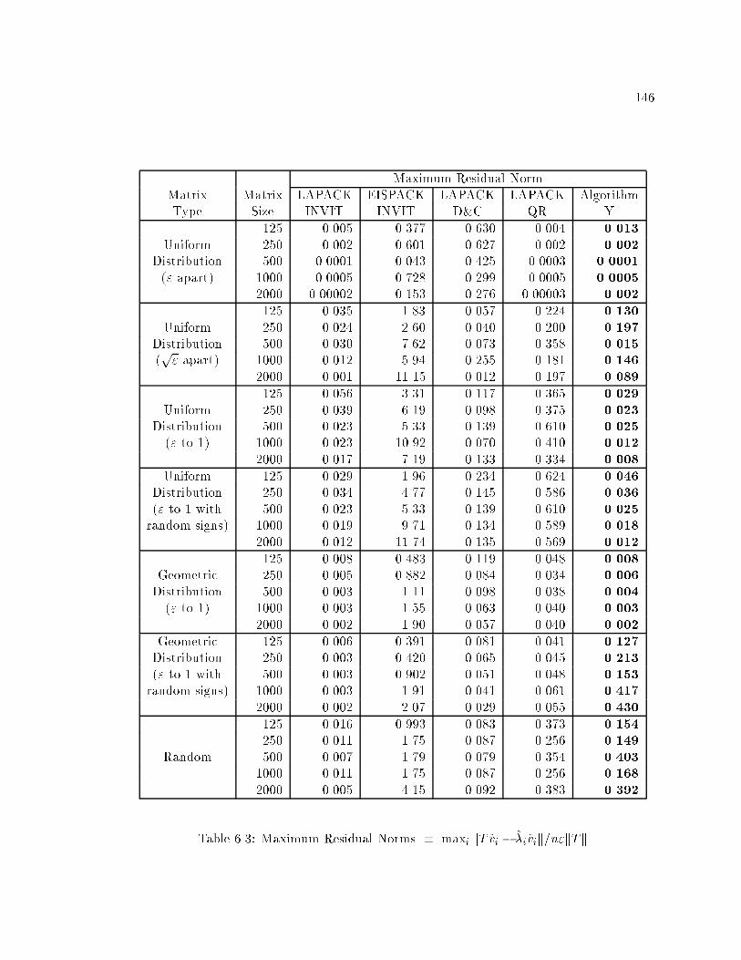
146
Maximum Residual Norm
Matrix Matrix LAPACK EISPACK LAPACK LAPACK Algorithm
Type Size INVIT INVIT D&C QR Y
125 0.005 0.377 0.630 0.004 0.013
Uniform 250 0.002 0.601 0.627 0.002 0.002
Distribution 500 0.0001 0.043 0.425 0.0003 0.0001
(" apart) 1000 0.0005 0.728 0.299 0.0005 0.0005
2000 0.00002 0.153 0.276 0.00003 0.002
125 0.035 1.83 0.057 0.224 0.130
Uniform 250 0.024 2.60 0.040 0.200 0.197
Distribution 500 0.030 7.62 0.073 0.358 0.015
(p" apart) 1000 0.012 5.94 0.255 0.181 0.146
2000 0.001 11.15 0.012 0.197 0.089
125 0.056 3.31 0.117 0.365 0.029
Uniform 250 0.039 6.19 0.098 0.375 0.023
Distribution 500 0.023 5.33 0.139 0.610 0.025
(" to 1) 1000 0.023 10.92 0.070 0.410 0.012
2000 0.017 7.19 0.133 0.334 0.008
Uniform 125 0.029 1.96 0.234 0.624 0.046
Distribution 250 0.034 4.77 0.145 0.586 0.036
(" to 1 with 500 0.023 5.33 0.139 0.610 0.025
random signs) 1000 0.019 9.71 0.134 0.589 0.018
2000 0.012 11.74 0.135 0.569 0.012
125 0.008 0.483 0.119 0.048 0.008
Geometric 250 0.005 0.882 0.084 0.034 0.006
Distribution 500 0.003 1.11 0.098 0.038 0.004
(" to 1) 1000 0.003 1.55 0.063 0.040 0.003
2000 0.002 1.90 0.057 0.040 0.002
Geometric 125 0.006 0.391 0.081 0.041 0.127
Distribution 250 0.003 0.420 0.065 0.045 0.213
(" to 1 with 500 0.003 0.902 0.051 0.048 0.153
random signs) 1000 0.003 1.91 0.041 0.061 0.417
2000 0.002 2.07 0.029 0.055 0.430
125 0.016 0.993 0.083 0.373 0.154
250 0.011 1.75 0.087 0.256 0.149
Random 500 0.007 1.79 0.079 0.354 0.403
1000 0.011 1.75 0.087 0.256 0.168
2000 0.005 4.15 0.092 0.383 0.392
Table 6.3: Maximum Residual Norms � maxi kT vi � �ivik=n"kTk
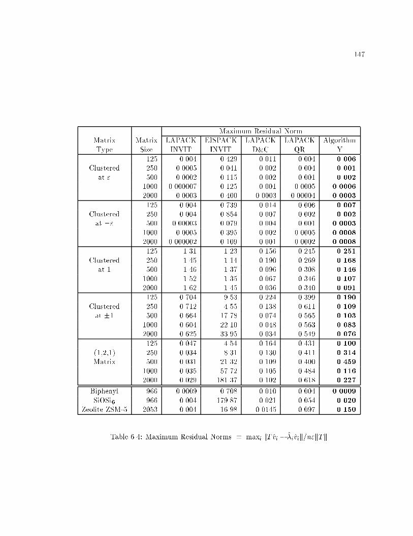
147
Maximum Residual Norm
Matrix Matrix LAPACK EISPACK LAPACK LAPACK Algorithm
Type Size INVIT INVIT D&C QR Y
125 0.004 0.429 0.011 0.004 0.006
Clustered 250 0.0005 0.041 0.002 0.004 0.001
at " 500 0.0002 0.115 0.002 0.001 0.002
1000 0.000007 0.125 0.001 0.0005 0.0006
2000 0.0003 0.400 0.0003 0.00004 0.0003
125 0.004 0.739 0.014 0.006 0.007
Clustered 250 0.004 0.854 0.007 0.002 0.002
at �" 500 0.00003 0.079 0.004 0.001 0.0003
1000 0.0005 0.395 0.002 0.0005 0.0008
2000 0.000002 0.109 0.001 0.0002 0.0008
125 1.31 1.23 0.156 0.245 0.251
Clustered 250 1.45 1.14 0.190 0.269 0.168
at 1 500 1.46 1.37 0.096 0.308 0.146
1000 1.52 1.35 0.067 0.346 0.107
2000 1.62 1.45 0.036 0.340 0.091
125 0.704 9.53 0.224 0.399 0.190
Clustered 250 0.712 4.55 0.138 0.611 0.109
at �1 500 0.664 17.78 0.074 0.565 0.103
1000 0.604 22.10 0.048 0.563 0.083
2000 0.625 33.95 0.034 0.549 0.076
125 0.047 4.54 0.164 0.431 0.100
(1,2,1) 250 0.034 8.31 0.130 0.411 0.314
Matrix 500 0.031 21.32 0.109 0.400 0.459
1000 0.035 57.72 0.105 0.484 0.116
2000 0.029 181.37 0.102 0.618 0.227
Biphenyl 966 0.0009 0.708 0.010 0.004 0.0009
SiOSi6 966 0.004 179.87 0.021 0.054 0.020
Zeolite ZSM-5 2053 0.004 16.98 0.0145 0.097 0.150
Table 6.4: Maximum Residual Norms � maxi kT vi � �ivik=n"kTk
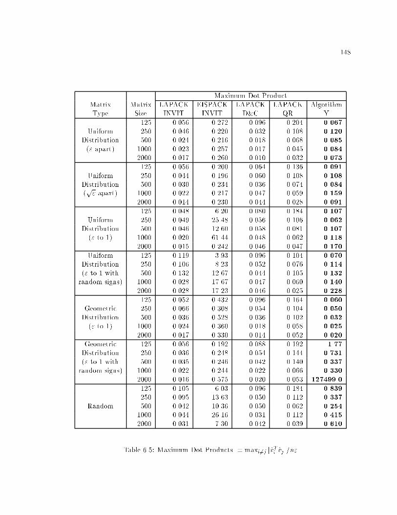
148
Maximum Dot Product
Matrix Matrix LAPACK EISPACK LAPACK LAPACK Algorithm
Type Size INVIT INVIT D&C QR Y
125 0.056 0.272 0.096 0.204 0.067
Uniform 250 0.046 0.220 0.032 0.108 0.120
Distribution 500 0.024 0.216 0.018 0.068 0.085
(" apart) 1000 0.023 0.257 0.017 0.045 0.084
2000 0.017 0.260 0.010 0.032 0.073
125 0.056 0.200 0.064 0.136 0.091
Uniform 250 0.044 0.196 0.060 0.108 0.108
Distribution 500 0.030 0.234 0.036 0.074 0.084
(p" apart) 1000 0.022 0.217 0.047 0.059 0.159
2000 0.014 0.230 0.044 0.028 0.091
125 0.048 6.20 0.080 0.184 0.107
Uniform 250 0.049 25.48 0.056 0.106 0.062
Distribution 500 0.046 12.60 0.058 0.081 0.107
(" to 1) 1000 0.020 61.44 0.048 0.062 0.118
2000 0.015 0.242 0.046 0.047 0.170
Uniform 125 0.119 3.93 0.096 0.104 0.070
Distribution 250 0.106 8.23 0.052 0.076 0.114
(" to 1 with 500 0.132 12.67 0.044 0.105 0.132
random signs) 1000 0.028 17.67 0.047 0.060 0.140
2000 0.028 17.23 0.046 0.025 0.228
125 0.052 0.432 0.096 0.164 0.060
Geometric 250 0.066 0.308 0.054 0.104 0.050
Distribution 500 0.036 0.528 0.036 0.102 0.032
(" to 1) 1000 0.024 0.360 0.018 0.058 0.025
2000 0.017 0.330 0.014 0.052 0.020
Geometric 125 0.056 0.192 0.088 0.192 1.77
Distribution 250 0.036 0.248 0.054 0.144 0.731
(" to 1 with 500 0.035 0.246 0.042 0.140 0.337
random signs) 1000 0.022 0.244 0.022 0.066 0.330
2000 0.016 0.575 0.020 0.053 127499.0
125 0.105 6.03 0.096 0.184 0.839
250 0.095 13.63 0.050 0.112 0.337
Random 500 0.042 10.36 0.050 0.062 0.254
1000 0.044 26.16 0.031 0.112 0.415
2000 0.031 7.30 0.042 0.039 0.610
Table 6.5: Maximum Dot Products � maxi6=j jvTi vj j=n"
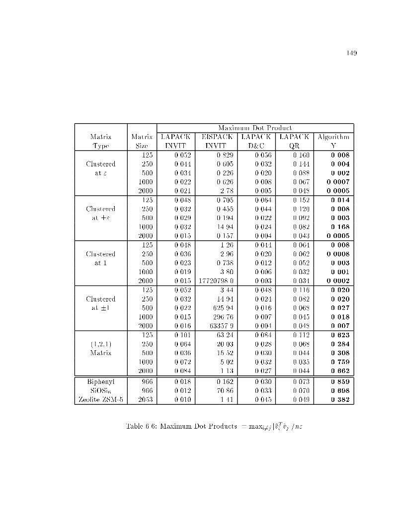
149
Maximum Dot Product
Matrix Matrix LAPACK EISPACK LAPACK LAPACK Algorithm
Type Size INVIT INVIT D&C QR Y
125 0.052 0.829 0.056 0.160 0.008
Clustered 250 0.044 0.605 0.032 0.144 0.004
at " 500 0.034 0.226 0.020 0.088 0.002
1000 0.022 0.626 0.008 0.067 0.0007
2000 0.021 2.78 0.005 0.048 0.0005
125 0.048 0.705 0.064 0.152 0.014
Clustered 250 0.032 0.455 0.044 0.120 0.008
at �" 500 0.029 0.194 0.022 0.092 0.003
1000 0.032 14.94 0.024 0.082 0.168
2000 0.015 0.157 0.004 0.043 0.0005
125 0.048 1.26 0.044 0.064 0.008
Clustered 250 0.036 2.96 0.020 0.062 0.0008
at 1 500 0.023 0.738 0.012 0.052 0.003
1000 0.019 3.80 0.006 0.032 0.001
2000 0.015 17720798.0 0.003 0.034 0.0002
125 0.052 3.44 0.048 0.116 0.020
Clustered 250 0.032 14.94 0.024 0.082 0.020
at �1 500 0.022 625.94 0.016 0.068 0.027
1000 0.015 296.76 0.007 0.045 0.018
2000 0.016 63357.9 0.004 0.048 0.007
125 0.101 63.24 0.084 0.112 0.623
(1,2,1) 250 0.064 20.03 0.028 0.068 0.284
Matrix 500 0.036 15.52 0.030 0.044 0.308
1000 0.072 5.02 0.032 0.035 0.759
2000 0.084 1.13 0.027 0.044 0.662
Biphenyl 966 0.018 0.162 0.030 0.073 0.859
SiOSi6 966 0.012 70.86 0.033 0.070 0.698
Zeolite ZSM-5 2053 0.010 1.41 0.045 0.049 0.382
Table 6.6: Maximum Dot Products � maxi6=j jvTi vj j=n"
150
invoking the ideas of Section 6.3, submatrices of very small size are needed by our new
algorithm to compute orthogonal eigenvectors. As a result, Algorithm Y takes as little
as 0:25 seconds to �nd all the eigenpairs of such a matrix of size 2000, while traditional
LAPACK inverse iteration takes 840 seconds. All our timing results con�rm Algorithm Y to
be an O(n2) method. The new technique of �nding the eigenvector of an isolated eigenvalue
by using twisted factorizations (see Chapter 3 for details) implies that our new algorithm is
faster even in cases that are favorable for EISPACK and LAPACK's inverse iteration, i.e.,
matrices of type 4 and type 7.
We mentioned the uncertainty in implementing certain steps of Algorithm Y at
the beginning of this chapter. The reason is the lack of a complete theory behind multiple
representations. This uncertainty has led to some redundancy and less than satisfactory �xes
(such as a tolerance on the acceptable element growth) in our preliminary code which will
hopefully be eliminated in the near future. In addition, whenever we form a relatively robust
representation we need to recompute the locally small eigenvalues to high relative accuracy.
Thus, even though it is still an O(n2) process, our code slows down somewhat when it needs
to form many representations. Due to these reasons, the matrix with eigenvalues arranged
in geometric order from " to 1 (with random signs) is the hardest one for Algorithm Y,
as evinced by the time needed and an occasionally larger than acceptable deviation from
orthogonality. In contrast, Algorithm Y performs very well on a similar type of matrix
where the eigenvalues are geometrically distributed from " to 1 (without any random signs
attached to them). The upcoming Section 6.5 lists some possible algorithmic improvements
that should remove this discrepancy in performance on these similar types of matrices.
Tables 6.3-6.6 show that the residual norms and orthogonality of the eigenpairs computed
by our current implementation of Algorithm Y are generally, very good.
The divide and conquer method is the fastest among all the earlier algorithms and
on examples where eigenvalues are close, it outperforms our preliminary implementation of
Algorithm Y. This success is due to the de ation process, where an eigenpair of a submatrix
is found to be an acceptable eigenpair of the full matrix. However, in cases where the
eigenvalues are well-separated, the divide and conquer algorithm takes O(n3) time and is
slower than Algorithm Y. One major drawback of LAPACK D&C is its extra workspace
requirement of more than 2n2 double precision words, which can be prohibitively excessive.
In fact, in the recent past, some people have turned to LAPACK INVIT instead of divide
and conquer to solve their large problems solely for this reason [6, 53, 52]. Of course,
151
workspace of only about 5-10 n double precision words is required by Algorithm Y, and
EISPACK and LAPACK INVIT.
The QR method is seen to uniformly take O(n3) time and is less sensitive to
the eigenvalue distribution. It is quite competitive with the other methods on matrices of
small size. Both the QR method and the divide and conquer algorithm produce accurate
eigenpairs, as seen from Tables 6.3, 6.4, 6.5 and 6.6.
We now discuss performance of the various algorithms on matrices that arise from
quantum chemistry applications. Table 6.2 shows that our Algorithm Y is the fastest
method for these matrices. In the results discussed above, the matrices were characterized
by their eigenvalue distributions. In Figures 6.1, 6.2 and 6.3, we did give the eigenvalues of
the three matrices under consideration. However, the quantities of interest are the absolute
and relative gaps between the eigenvalues. The left halves of Figures 6.4, 6.5 and 6.6 plot
the logarithms of absolute gaps, i.e.,
log10
�absgap(i)
kTk�
= log10
�min(�i+1 � �i; �i � �i�1)
kTk�; (6.4.5)
while the right halves plot the relative gaps on a logarithmic scale, i.e.,
log10 (relgap(i)) = log10
�min(�i+1 � �i; �i � �i�1)
j�ij�: (6.4.6)
Recall that in (6.4.5) and (6.4.6), the eigenvalues are arranged in ascending order.
From Figure 6.4, we see that almost all the absolute gaps for the biphenyl matrix
are less than 10�3kTk and consequently, both LAPACK and EISPACK INVIT spend O(n3)
time on this matrix of order 966. Most of the eigenvalues, however, agree in less than 3
leading digits and as a result, Algorithm Y is about 10 times faster than LAPACK INVIT.
This translates to a 3-fold increase in speed of the total dense symmetric eigenproblem.
Similar behavior is observed in the SiOSi6 matrix. We see a di�erent distribution in the
Zeolite example where the relative gaps are similar to the absolute gaps. Despite the need
to form many representations, we observe that Algorithm Y is still faster than the earlier
methods.
We have also implemented a parallel variant of Algorithm Y in collaboration with
computational chemists at Paci�c Northwest National Laboratories (PNNL). This will re-
place the earlier tridiagonal eigensolver based on inverse iteration that was part of the
PeIGS version 2.0 library [52]. Our new method is more easily parallelized, and coupled
with its lower operation count, o�ers an even bigger computational advantage on a parallel
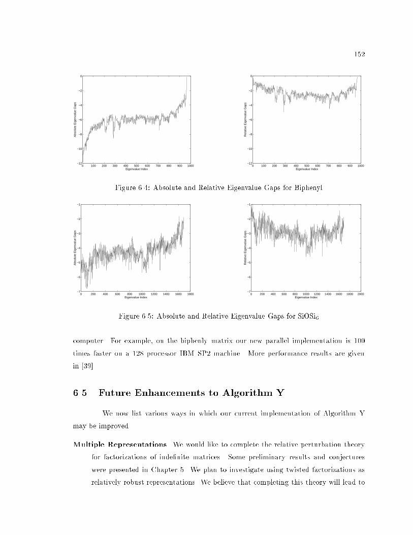
152
0 100 200 300 400 500 600 700 800 900 1000−12
−10
−8
−6
−4
−2
0
Eigenvalue Index
Abs
olut
e E
igen
valu
e G
aps
0 100 200 300 400 500 600 700 800 900 1000−12
−10
−8
−6
−4
−2
0
Eigenvalue Index
Rel
ativ
e E
igen
valu
e G
aps
Figure 6.4: Absolute and Relative Eigenvalue Gaps for Biphenyl
0 200 400 600 800 1000 1200 1400 1600 1800−7
−6
−5
−4
−3
−2
−1
Eigenvalue Index
Abs
olut
e E
igen
valu
e G
aps
0 200 400 600 800 1000 1200 1400 1600 1800 2000−7
−6
−5
−4
−3
−2
−1
Eigenvalue Index
Rel
ativ
e E
igen
valu
e G
aps
Figure 6.5: Absolute and Relative Eigenvalue Gaps for SiOSi6
computer. For example, on the biphenly matrix our new parallel implementation is 100
times faster on a 128 processor IBM SP2 machine. More performance results are given
in [39].
6.5 Future Enhancements to Algorithm Y
We now list various ways in which our current implementation of Algorithm Y
may be improved.
Multiple Representations. We would like to complete the relative perturbation theory
for factorizations of inde�nite matrices. Some preliminary results and conjectures
were presented in Chapter 5. We plan to investigate using twisted factorizations as
relatively robust representations. We believe that completing this theory will lead to
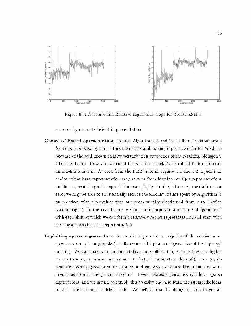
153
0 500 1000 1500 2000 2500−10
−9
−8
−7
−6
−5
−4
−3
−2
−1
0
Eigenvalue Index
Abs
olut
e E
igen
valu
e G
aps
0 500 1000 1500 2000 2500−10
−9
−8
−7
−6
−5
−4
−3
−2
−1
0
Eigenvalue Index
Rel
ativ
e E
igen
valu
e G
aps
Figure 6.6: Absolute and Relative Eigenvalue Gaps for Zeolite ZSM-5
a more elegant and e�cient implementation.
Choice of Base Representation. In both Algorithms X and Y, the �rst step is to form a
base representation by translating the matrix and making it positive de�nite. We do so
because of the well known relative perturbation properties of the resulting bidiagonal
Cholesky factor. However, we could instead form a relatively robust factorization of
an inde�nite matrix. As seen from the RRR trees in Figures 5.1 and 5.2, a judicious
choice of the base representation may save us from forming multiple representations
and hence, result in greater speed. For example, by forming a base representation near
zero, we may be able to substantially reduce the amount of time spent by Algorithm Y
on matrices with eigenvalues that are geometrically distributed from " to 1 (with
random signs). In the near future, we hope to incorporate a measure of \goodness"
with each shift at which we can form a relatively robust representation, and start with
the \best" possible base representation.
Exploiting sparse eigenvectors. As seen in Figure 4.6, a majority of the entries in an
eigenvector may be negligible (this �gure actually plots an eigenvector of the biphenyl
matrix). We can make our implementation more e�cient by setting these negligible
entries to zero, in an a priori manner. In fact, the submatrix ideas of Section 6.3 do
produce sparse eigenvectors for clusters, and can greatly reduce the amount of work
needed as seen in the previous section. Even isolated eigenvalues can have sparse
eigenvectors, and we intend to exploit this sparsity and also push the submatrix ideas
further to get a more e�cient code. We believe that by doing so, we can get an
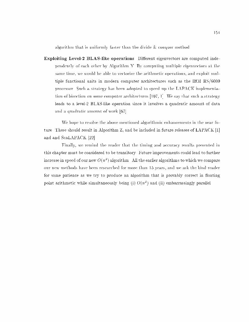
154
algorithm that is uniformly faster than the divide & conquer method.
Exploiting Level-2 BLAS-like operations. Di�erent eigenvectors are computed inde-
pendently of each other by Algorithm Y. By computing multiple eigenvectors at the
same time, we would be able to vectorize the arithmetic operations, and exploit mul-
tiple functional units in modern computer architectures such as the IBM RS/6000
processor. Such a strategy has been adopted to speed up the LAPACK implementa-
tion of bisection on some computer architectures [107, 1]. We say that such a strategy
leads to a level-2 BLAS-like operation since it involves a quadratic amount of data
and a quadratic amount of work [67].
We hope to resolve the above mentioned algorithmic enhancements in the near fu-
ture. These should result in Algorithm Z, and be included in future releases of LAPACK [1]
and and ScaLAPACK [22].
Finally, we remind the reader that the timing and accuracy results presented in
this chapter must be considered to be transitory. Future improvements could lead to further
increase in speed of our new O(n2) algorithm. All the earlier algorithms to which we compare
our new methods have been researched for more than 15 years, and we ask the kind reader
for some patience as we try to produce an algorithm that is provably correct in oating
point arithmetic while simultaneously being (i) O(n2) and (ii) embarrassingly parallel.
155
Chapter 7
Conclusions
In this thesis, we have shown how to compute numerically orthogonal approxi-
mations to eigenvectors without resorting to any reorthogonalization technique such as the
Gram-Schmidt process. Consequently, our new algorithm can compute orthogonal eigen-
vectors in O(n2) time. The individual eigenvectors are computed independently of each
other which is well-suited for parallel computation. Moreover, our algorithm can deliver
any subset of the eigenvalues and eigenvectors at a cost of O(n) operations per eigenpair.
We now discuss some of the guiding principles behind the advances mentioned
above. We feel that these principles are general in the sense that they could be applied to
other numerical procedures. In the following, we list these principles and show how we have
applied them to get a faster O(n2) solution to the tridiagonal eigenproblem.
Do not try to compute a quantity that is not well-determined. When eigenvalues
are close, individual eigenvectors are extremely sensitive to small changes in the ma-
trix entries. On the other hand, the invariant subspace corresponding to these close
eigenvalues is well-determined and any orthogonal basis of this subspace will su�ce
as approximate eigenvectors. Earlier EISPACK and LAPACK software attempt to
compute such a (non-unique) basis by explicit orthogonalization and hence, can take
O(n3) time. However, as explained in Chapter 5, we have been able to �nd alter-
nate representations of the initial matrix so that the re�ned eigenvalues are no longer
\close" and the corresponding eigenvectors are now well-determined. These new rep-
resentations allow us to identify a robust orthogonal basis of the desired subspace and
hence, compute it cheaply. Another major advance in our methods comes by recog-
nizing that the bidiagonal factors of a tridiagonal determine the desired quantities
156
much \better" than its diagonal and o�-diagonal entries.
Exploiting transformations for which the solution is invariant. Eigenvalues of a ma-
trix A are invariant under the similarity transformations S�1AS, and change in a sim-
ple way under a�ne transformations of the form �A+�, � 6= 0. Several methods such
as the QR, LR and qd algorithms take advantage of such transformations. Eigenvec-
tors of A are easily seen to be invariant under any a�ne transformation. We exploit
this property to great advantage by obtaining various representations of the given
problem, each of which is \better" suited for computing a subset of the spectrum.
Finding \good" representations. We need to make sure that the above transformations
do not a�ect the accuracy of the desired quantities. Thus to produce eigenpairs that
have small residual norms, as speci�ed in (1.1.1), we need to avoid large element
growths in forming the intermediate factorizations
T � �I = LDLT : (7.0.1)
See Chapter 5 for details.
High Accuracy in key computations can lead to speed. The main reason for form-
ing multiple representations, as in (7.0.1), is to avoid Gram-Schmidt like methods in
computing orthogonal approximations to the eigenvectors. Our faster O(n2) scheme
becomes possible only because the intermediate representations determine their small
eigenvalues to high relative accuracy. We can then compute these small eigenvalues
to full relative accuracy and use these highly accurate eigenvalues to compute eigen-
vectors. The resulting eigenvectors we compute are \faithful" and orthogonal as a
consequence. In numerical methods, there is generally believed to be a trade-o� be-
tween speed and accuracy, i.e., higher accuracy can be achieved only at the expense
of computing time. However, we have demonstrated that high accuracy in the right
places can actually speed up the computation.
7.1 Future Work
In Section 6.5, we mentioned further enhancements to Algorithm Y which we
intend to incorporate in the near future. Here we see how some of our ideas may be applied
to other problems in numerical linear algebra.
157
Perfect Shifts. In Section 3.5.1 we showed how to e�ectively use the perfect shift strategy
in a QR-like algorithm. This new scheme enables us to use \ultimate" or \perfect"
shifts as envisaged by Parlett in [110]. It also solves the problem of immediately
de ating a known eigenpair from a symmetric matrix by deleting one of its rows and
columns. We intend to substantiate these claims with numerical experiments in the
near future [41].
Non-symmetric Eigenproblem. Since Algorithm Y does not invoke any Gram-Schmidt
like process, it does not explicitly try to compute eigenvectors that are orthogonal.
Orthogonality is a result of the matrix being symmetric. We believe that many of
our ideas can be applied to the non-symmetric eigenproblem in order to obtain the
\best-conditioned" eigenvectors.
Lanczos Algorithm. The method proposed by Lanczos in 1952 [97], after many modi-
�cations to account for roundo� [125, 110, 126], has become the champion among
algorithms to �nd some of the extreme eigenvalues of a sparse symmetric matrix. It
proceeds by incrementally forming, one row and column at a time, a tridiagonal ma-
trix that is similar to the sparse matrix. We would like to investigate if there are any
bene�ts in using the LDLT decomposition of this tridiagonal or its translates. The
sparsity of the eigenvectors of the tridiagonal, see Figure 4.6 for an example, may also
be exploited in reducing the amount of work in the selective orthogonalization phase.
See [125] for details on the latter phase.
Rank-Revealing Factorizations. The twisted factorizations introduced in Section 3.1
enable us to accurately compute a null vector of a nearly singular tridiagonal matrix.
The particular twisted factorization used is successful because it transparently reveals
the near singularity of the tridiagonal. As discussed in Section 3.6, twisted factoriza-
tions can also be formed for denser matrices. A nice property is that they tend to
preserve the sparsity pattern of the matrix. Coupled with their rank-revealing prop-
erties, twisted factorizations may become an invaluable computational tool in banded
(sparse) matrix computations.
158
Bibliography
[1] E. Anderson, Z. Bai, C. Bischof, J. Demmel, J. Dongarra, J. Du Croz, A. Greenbaum, S. Ham-
marling, A. McKenney, S. Ostrouchov, and D. Sorensen. LAPACK Users' Guide (second
edition). SIAM, Philadelphia, 1995. 324 pages.
[2] ANSI/IEEE, New York. IEEE Standard for Binary Floating Point Arithmetic, Std 754-1985
edition, 1985.
[3] P. Arbenz, K. Gates, and Ch. Sprenger. A parallel implementation of the symmetric tridiagonal
QR algorithm. In Frontier's 92. McLean, 1992.
[4] S. O. Asplund. Finite boundary value problems solved by Green's matrix. Math. Scand.,
7:49{56, 1959.
[5] I. Babuska. Numerical stability in problems of linear algebra. SIAM J. Num. Anal., 9:53{77,
1972.
[6] Z. Bai, 1996. private communication.
[7] V. Bargmann, D. Montgomery, and J. von Neumann. Solution of linear systems of high order.
Report prepared for Navy Bureau of Ordnance, 1946. Reprinted in [131, pp. 421{477].
[8] J. Barlow, 1996. private communication.
[9] J. Barlow and J. Demmel. Computing accurate eigensystems of scaled diagonally dominant
matrices. SIAM J. Num. Anal., 27(3):762{791, June 1990.
[10] D. Bernholdt and R. Harrison. Orbital invariant second order many-body perturbation on
parallel computers: An approach for large molecules. J. Chem. Physics., 1995.
[11] H. J. Bernstein and M. Goldstein. Parallel implementation of bisection for the calculation of
eigenvalues of a tridiagonal symmetric matrices. Computing, 37:85{91, 1986.
[12] Christian H. Bischof and Charles F. Van Loan. The WY representation for products of House-
holder matrices. SIAM J. Sci. Stat. Comput., 8(1):s2{s13, 1987.
[13] R. P. Brent. Algorithms for minimization without derivatives. Prentice-Hall, 1973.
159
[14] B. Bukhberger and G.A. Emel'yanenko. Methods of inverting tridiagonal matrices. USSR
Computat. Math. and Math. Phy., 13:10{20, 1973.
[15] J. Bunch, P. Nielsen, and D. Sorensen. Rank-one modi�cation of the symmetric eigenproblem.
Num. Math., 31:31{48, 1978.
[16] J. Carrier, L. Greengard, and V. Rokhlin. A fast adaptive multipole algorithm for particle
simulations. SIAM, J. Sci. Stat. Comput., 9(4):669{686, July 1988.
[17] S. Chakrabarti, J. Demmel, and K. Yelick. Modeling the bene�ts of mixed data and task
parallelism. In Symposium on Parallel Algorithms and Architectures (SPAA), Santa Barbara,
California, july 1995.
[18] T. Chan. Rank revealing QR factorizations. Lin. Alg. Appl., 88/89:67{82, 1987.
[19] T. F. Chan. On the existence and computation of LU-factorizations with small pivots. Math.
Comp., 42:535{547, 1984.
[20] S. Chandrasekaran. When is a Linear System Ill-Conditioned? PhD thesis, Departement of
Computer Science, Yale University, New Haven, CT, 1994.
[21] Bruce W. Char, Keith O. Geddes, Gaston H. Gonnet, Benton L. Leong, Michael B. Monagan,
and Stephen M. Watt. Maple V Library Reference Manual. Springer-Verlag, Berlin, 1991.
[22] J. Choi, J. Demmel, I. Dhillon, J. Dongarra, Ostrouchov, S., A. Petitet, K. Stanley, D. Walker,
and R. C. Whaley. ScaLAPACK, a portable linear algebra library for distributed memory
computers-design issues and performance. Computer Physics Communications, 97(1-2):1{15,
1996.
[23] M. Chu. A simple application of the homotopy method to symmetric eigenvalue problems.
Lin. Alg. Appl, 59:85{90, 1984.
[24] M. Chu. A note on the homotopy method for linear algebraic eigenvalue problems. Lin. Alg.
Appl, 105:225{236, 1988.
[25] J.J.M. Cuppen. A divide and conquer method for the symmetric tridiagonal eigenproblem.
Numer. Math., 36:177{195, 1981.
[26] C. Davis and W. Kahan. Some new bounds on perturbation of subspaces. Bulletin of the
American Mathematical Society, 77(4):863{868, July 1969.
[27] C. Davis and W. Kahan. The rotation of eigenvectors by a perturbation III. SIAM J. Num.
Anal., 7:248{263, 1970.
[28] D. Day. The di�erential qd algorithm for the tridiagonal eigenvalue problem. 1997. in prepa-
ration.
160
[29] P. Deift, J. Demmel, L.-C. Li, and C. Tomei. The bidiagonal singular values decomposition
and Hamiltonianmechanics. SIAM J. Num. Anal., 28(5):1463{1516, October 1991. (LAPACK
Working Note #11).
[30] L. S. DeJong. Towards a formal de�nition of numerical stability. Numer. Math., 28:211{220,
1977.
[31] T. J. Dekker. Finding a zero by means of successive linear interpolation. In B. Dejon and
P. Henrici, editors, Constructive aspects of the fundamanetal theorem of algebra. New York:
Wiley-Interscience, 1969.
[32] J. Demmel. The inherent inaccuracy of implicit tridiagonal QR. Technical Report Report 963,
IMA, University of Minnesota, April 1992.
[33] J. Demmel and W. Gragg. On computing accurate singular values and eigenvalues of acyclic
matrices. Lin. Alg. Appl., 185:203{218, 1993.
[34] J. Demmel, M. Gu, S. Eisenstat, I. Slapni�car, K. Veseli�c, and Z. Drma�c. Computing the
singular value decomposition with high relative accuracy. Computer Science Dept. Technical
Report CS-97-348, University of Tennessee, Knoxville, February 1997. (LAPACK Working
Note #119, available electronically on netlib).
[35] J. Demmel and W. Kahan. Accurate singular values of bidiagonal matrices. SIAM J. Sci.
Stat. Comput., 11(5):873{912, September 1990.
[36] J. Demmel and A. McKenney. A test matrix generation suite. Computer science dept. technical
report, Courant Institute, New York, NY, July 1989. (LAPACK Working Note #9).
[37] J. Demmel and K. Veseli�c. Jacobi's method is more accurate than QR. SIAM J. Mat. Anal.
Appl., 13(4):1204{1246, 1992. (also LAPACK Working Note #15).
[38] J. W. Demmel. personal communication, 1996.
[39] I. Dhillon, G. Fann, and B. Parlett. Application of a new algorithm for the symmetric eigen-
problem to computational quantum chemistry. In Proceedings of the Eighth SIAM Conference
on Parallel Proceesing for Scienti�c Computing. SIAM, March 1997.
[40] I. S. Dhillon. Current inverse iteration software can fail. 1997. Submitted for publication.
[41] I. S. Dhillon. Perfect shifts and twisted factorizations. 1997. In preparation.
[42] I. S. Dhillon. Stable computation of the condition number of a tridiagonal matrix in O(n)
time. 1997. Submitted for publication.
[43] I. S. Dhillon and B.N. Parlett. Orthogonal eigenvectors without Gram-Schmidt. 1997. in
preparation.
161
[44] J. Dongarra, J. Bunch, C. Moler, and G. W. Stewart. LINPACK User's Guide. SIAM,
Philadelphia, PA, 1979.
[45] J. Dongarra, J. Du Croz, I. Du�, and S. Hammarling. A set of Level 3 Basic Linear Algebra
Subprograms. ACM Trans. Math. Soft., 16(1):1{17, March 1990.
[46] J. Dongarra and D. Sorensen. A fully parallel algorithm for the symmetric eigenproblem.
SIAM J. Sci. Stat. Comput., 8(2):139{154, March 1987.
[47] J. Dongarra, R. van de Geijn, and D. Walker. A look at scalable dense linear algebra libraries.
In Scalable High-Performance Computing Conference. IEEE Computer Society Press, April
1992.
[48] J. DuCroz, December 1994. private communication.
[49] S. Eisenstat and I. Ipsen. Relative perturbation techniques for singular value problems. SIAM
J. Numer. Anal., 32(6), 1995.
[50] S. C. Eisenstat and I. C. F. Ipsen. Relative perturbation bounds for eigenspaces and singular
vector subspaces. In J. G. Lewis, editor, Proceedings of the Fifth SIAM Conference on Applied
Linear Algebra, pages 62{65. SIAM, 1994.
[51] S.C. Eisenstat and I.C.F. Ipsen. Relative perturbation results for eigenvalues and eigenvectors
of diagonalisable matrices. Technical Report CRSC-TR96-6, Center for Research in Scienti�c
Computation, Department of Mathematics, North Carolina State University, 1996. (14 pages).
[52] D. Elwood, G. Fann, and D. Little�eld. PeIGS User's Manual. Paci�c Northwest National
Laboratory, Richland, WA, 1993.
[53] G.I. Fann, 1996. private communication.
[54] G.I. Fann and R. J. Little�eld. Parallel inverse iteration with re-orthogonalization. In R. Sin-
covec et. al., editor, Proceedings of the Sixth SIAM Conference on Parallel Processing for
Scienti�c Computing, volume 1, pages 409{413. SIAM, 1993.
[55] G.I. Fann, R. J. Little�eld, and D.M. Elmwood. Performance of a fully parallel dense real
symmetric eigensolver in quantum chemistry appliacation. In Proceedings of the High Per-
formance Computing '95, Simulation MultiConference. The Society of Computer Simulation,
San Diego, 1995.
[56] K. Fernando and B. Parlett. Accurate singular values and di�erential qd algorithms. Nu-
merische Mathematik, 67:191{229, 1994.
[57] K. V. Fernando. On computing an eigenvector of a tridiagonal matrix. Technical Report
TR4/95, Nag Ltd., Oxford, UK, 1995. submitted for publication.
162
[58] D. Fischer, G. H. Golub, O. Hald, C. Leiva, and O. Widlund. On Fourier Toeplitz methods
for separable elliptic problems. Math. Comp., 28:349{368, 1974.
[59] G. J. F. Francis. The QR transformation, parts I and II. Computer J., 4:265{271,332{345,
1961-62.
[60] K. E. Gates. Using inverse iteration to improve the divide and conquer algorithm. Technical
Report 159, ETH Department Informatik, May 1991.
[61] W. Givens. The characteristic value-vector problem. J. ACM, 4:298{307, 1957. also unpub-
lished report.
[62] Wallace J. Givens. Numerical computation of the characteristic values of a real symmetric
matrix. Technical Report ORNL-1574, Oak Ridge National Laboratory, Oak Ridge, TN, USA,
1954.
[63] S. K. Godunov, A. G. Antonov, O. P. Kiriljuk, and V. I. Kostin. Guaranted Accuracy in
Numerical Linear Algebra. Kluwer Academic Publishers, Dordrecht, Netherlands, 1993. A
revised translation of a Russian text �rst published in 1988 in Novosibirsk.
[64] S. K. Godunov, V. I. Kostin, and A. D. Mitchenko. Computation of an eigenvector of sym-
metric tridiagonal matrices. Siberian Math. J., 26:71{85, 1985.
[65] D. Goldberg. What every computer scientist should know about oating point arithmetic.
ACM Computing Surveys, 23(1), 1991.
[66] G. H. Golub, V. Klema, and G. W. Stewart. Rank degeneracy and least squares problems.
Technical Report STAN-CS-76-559, Computer Science Dept., Stanford Univ., 1976.
[67] Gene H. Golub and Charles F. Van Loan. Matrix computations. Johns Hopkins Studies in
the Mathematical Sciences. The Johns Hopkins University Press, Baltimore, MD, USA, third
edition, 1996.
[68] Ronald L. Graham, Donald E. Knuth, and Oren Patashnik. Concrete Mathematics: A Foun-
dation for Computer Science. Addison-Wesley, Reading, MA, USA, 1989.
[69] A. Greenbaum and J. Dongarra. Experiments with QL/QR methods for the symmetric tridi-
agonal eigenproblem. Computer Science Dept. Technical Report CS-89-92, University of Ten-
nessee, Knoxville, 1989. (LAPACK Working Note #17, available electronically on netlib).
[70] L. Greengard and V. Rokhlin. A fast algorithm for particle simulations. J. Comp. Phys.,
73:325{348, 1987.
[71] M. Gu. Studies in numerical linear algebra. Ph.D. thesis, 1993.
163
[72] M. Gu and S. C. Eisenstat. A stable and e�cient algorithm for the rank-1 modi�cation of the
symmetric eigenproblem. SIAM J. Mat. Anal. Appl., 15(4):1266{1276, October 1994. Yale
Tech report YALEU/DCS/RR-916, Sept 1992.
[73] M. Gu and S. C. Eisenstat. A divide-and-conquer algorithm for the symmetric tridiagonal
eigenproblem. SIAM J. Mat. Anal. Appl., 16(1):172{191, January 1995.
[74] F. G. Gustavson and A. Gupta. A new parallel algorithm for tridiagonal symmetric positive
de�nite systems of equations. unpublished report, 1996.
[75] B. Hendrickson, E. Jessup, and C. Smith. A parallel eigensolver for dense symmetric matrices.
Technical Report SAND96{0822, Sandia National Labs, Albuquerque, NM, March 1996.
[76] P. Henrici. The quotient-di�erence algorithm. Nat. Bur. Standards Appl. Math. Series, 19:23{
46, 1958.
[77] P. Henrici. Bounds for eigenvalues of certain tridiagonal matrices. SIAM J., 11:281{290, 1963.
[78] N. J. Higham. E�cient algorithms for computing the condition number of a tridiagonal matrix.
SIAM J. Sci. Stat. Comput., 7:150{165, 1986.
[79] Ho�man and B. N. Parlett. A new proof of global convergence for the tridiagonalQL algorithm.
SIAM J. Num. Anal., 15:929{937, 1978.
[80] R. A. Horn and C. R. Johnson. Matrix Analysis. Cambridge University Press, Cambridge,
1985. Includes Ostrowski's relative perturbation theory on pp 224-225.
[81] Alston S. Householder. Unitary triangularization of a nonsymmetric matrix. J. Assoc. Comput.
Mach., 5:339{342, 1958.
[82] IBM. Engineering and Scienti�c Subroutine Library, Guide and Reference, Release 3, Program
5668-863, 4 edition, 1988.
[83] I. Ikebe. On inverses of Hessenberg matrices. Linear Algebra and its Applications, 24:93{97,
1979.
[84] I. Ipsen and E. Jessup. Solving the symmetric tridiagonal eigenvalue problem on the hypercube.
SIAM J. Sci. Stat. Comput., 11(2):203{230, 1990.
[85] I. C. F. Ipsen. Computing an eigenvector with inverse iteration. SIAM Review, 1997. to
appear.
[86] C. G. F. Jacobi. Concerning an easy process for solving equations occurring in the theory of
secular disturbances. J. Reine Angnew. Math., 30:51{94, 1846.
[87] E. Jessup and I. Ipsen. Improving the accuracy of inverse iteration. SIAM J. Sci. Stat.
Comput., 13(2):550{572, 1992.
164
[88] E. R. Jessup. Parallel Solution of the Symmetric Tridiagonal Eigenproblem. PhD thesis, Yale
University, New Haven, CT, 1989.
[89] W. Kahan. Accurate eigenvalues of a symmetric tridiagonal matrix. Computer Science Dept.
Technical Report CS41, Stanford University, Stanford, CA, July 1966 (revised June 1968).
[90] W. Kahan. Notes on Laguerre's iteration. University of California Computer Science Division
preprint, 1992.
[91] W. Kahan. Lecture notes on the status of IEEE standard 754 for binary oating point arith-
metic. http://HTTP.CS.Berkeley.EDU/ wkahan/ieee754status/ieee754.ps, 1995.
[92] W. Kahan, 1996. private communication.
[93] L. Kaufman. A parallel QR algorithm for the symmetric tridiagonal eigenvalue problem. J.
of Parallel and Distributed Computing, 23(3):429{434, December 1994.
[94] D. Kershaw. Inequalities on elements of the inverse of a certain tridiagonal matrix.
Math. Comp., 24:155{158, 1970.
[95] V. N. Kublanovskaya. On some algorithms for the solution of the complete eigenvalue problem.
Zh. Vych. Mat., 1:555{570, 1961.
[96] D. Kuck and A. Sameh. A parallel QR algorithm for symmetric tridiagonal matrices. IEEE
Trans. Computers, C-26(2), 1977.
[97] C. Lanczos. Solution of systems of linear equations by minimized iterations. J. Res. Natl.
Bur. Stand, 49:33{53, 1952.
[98] J. Le and B. Parlett. Forward instability of tridiagonal QR. SIAM J. Mat. Anal. Appl.,
14(1):279{316, January 1993.
[99] K. Li and T.-Y. Li. An algorithm for symmetric tridiagonal eigenproblems | divide and
conquer with homotopy continuation. SIAM J. Sci. Comp., 14(3), May 1993.
[100] R.-C. Li. Relative perturbation theory: (I) eigenvalue and singular value variations. Technical
Report UCB//CSD-94-855, Computer Science Division, Department of EECS, University of
California at Berkeley, 1994. (revised January 1996).
[101] R.-C. Li. Relative perturbation theory: (II) eigenspace and singular subspace variations.
Technical Rep University of California at Berkeley UCB//CSD-94-856, Computer Science
Division, Department of EECS, University of California at Berkeley, 1994. (revised January
1996 and April 1996).
[102] R.-C. Li. Solving secular equations stably and e�ciently. Computer Science Dept. Technical
Report CS-94-260, University of Tennessee, Knoxville, November 1994. (LAPACK Working
Note #89).
165
[103] T.-Y. Li and N. H. Rhee. Homotopy algorithm for symmetric eigenvalue problems. Num.
Math., 55:265{280, 1989.
[104] T. Y. Li and Z. Zeng. The Laguerre iteration in solving the symmetric tridiagonal eigenprob-
lem, revisited. SIAM J. Sci. Stat. Comput., 15(5):1145{1173, September 1994.
[105] T.-Y. Li, H. Zhang, and X. H. Sun. Parallel homotopy algorithm for symmetric tridiagonal
eigenvalue problems. SIAM J. Sci. Stat. Comput., 12:464{485, 1991.
[106] S.-S. Lo, B. Phillipe, and A. Sameh. A multiprocessor algorithm for the symmetric eigenprob-
lem. SIAM J. Sci. Stat. Comput., 8(2):155{165, March 1987.
[107] A. McKenney, 1997. private communication.
[108] G. Meurant. A review on the inverse of symmetric tridiagonal and block tridiagonal matrices.
SIAM J. Mat. Anal. Appl., 13(3):707{728, July 1992.
[109] J. M. Ortega and H. F. Kaiser. The LLT and QRMethods for Symmetric TridiagonalMatrices.
Numer. Math., 5:211{225, 1963.
[110] B. Parlett. The Symmetric Eigenvalue Problem. Prentice Hall, Englewood Cli�s, NJ, 1980. A
new SIAM edition is under preparation.
[111] B. Parlett. Acta Numerica, chapter The new qd algorithms, pages 459{491. Cambridge
University Press, 1995.
[112] B. Parlett. The construction of orthogonal eigenvectors for tight clusters by use of submatrices.
Center for Pure and Applied Mathematics PAM-664, University of California, Berkeley, CA,
January 1996. submitted to SIMAX.
[113] B. N. Parlett. Laguerre's Method Applied to the Matrix Eigenvalue Problem. Math. Comp.,
18:464{485, 1964.
[114] B. N. Parlett. The rewards for maintaining semi-orthogonality among Lanczos vectors. Journal
of Numerical Linear Algebra with Applications, 1(2):243{267, 1992.
[115] B. N. Parlett. Invariant subspaces for tightly clustered eigenvalues of tridiagonals. BIT,
36(3):542{562, 1996.
[116] B. N. Parlett. Spectral sensitivity of products of bidiagonals. Linear Algebra and its Appli-
cations, 1996. submitted for inclusion in the proceedings of the 6th ILAS conference held in
Chemnitz, Germany in August 1996.
[117] B.N. Parlett and I.S. Dhillon. Fernando's solution to Wilkinson's problem: an application of
double factorization. Linear Algebra and its Applications, 1997. to appear.
166
[118] G. Peters and J.H. Wilkinson. The calculation of speci�ed eigenvectors by inverse itera-
tion, contribution II/18, volume II of Handbook of Automatic Computation, pages 418{439.
Springer-Verlag, New York, Heidelberg, Berlin, 1971.
[119] G. Peters and J.H. Wilkinson. Inverse iteration, ill-conditioned equations and Newton's
method. SIAM Review, 21:339{360, 1979.
[120] D. Priest. Algorithms for arbitrary precision oating point arithmetic. In P. Kornerup and
D. Matula, editors, Proceedings of the 10th Symposium on Computer Arithmetic, pages 132{
145, Grenoble, France, June 26-28 1991. IEEE Computer Society Press.
[121] H. Rutishauser. Der Quotienten-Di�erenzen-Algorithmus. Z. Angew. Math. Phys., 5:223{251,
1954.
[122] H. Rutishauser. Vorlesungen �uber numerische Mathematik. Birkh�auser, Basel, 1976.
[123] H. Rutishauser. Lectures on Numerical Mathematics. Birkh�auser, Boston, 1990.
[124] J. Rutter. A serial implementation of Cuppen's divide and conquer algorithm for the sym-
metric eigenvalue problem. Mathematics Dept. Master's Thesis available by anonymous ftp
to tr-ftp.cs.berkeley.edu, directory pub/tech-reports/csd/csd-94-799, �le all.ps, University of
California, 1994.
[125] D. Scott. Analysis of the Symmetric Lanczos Algorithm. PhD thesis, University of California,
Berkeley, California, 1978.
[126] H. Simon. The Lanczos algorithmwith partial reorthogonalization.Math. Comp., 42(165):115{
142, January 1984.
[127] H. Simon. Bisection is not optimal on vector processors. SIAM J. Sci. Stat. Comput.,
10(1):205{209, January 1989.
[128] B. T. Smith, J. M. Boyle, J. J. Dongarra, B. S. Garbow, Y. Ikebe, V. C. Klema, and C. B.
Moler. Matrix Eigensystem Routines { EISPACK Guide, volume 6 of Lecture Notes in Com-
puter Science. Springer-Verlag, Berlin, 1976.
[129] G. W. Stewart. Introduction to Matrix Computations. Academic Press, New York, 1973.
[130] W. G. Strang. Implicit di�erence methods for initial boundary value problems. J. Math. Anal.
Appl., 16:188{198, 1966.
[131] A. H. Taub, editor. John von Neumann Collected Works, volume V, Design of Computers,
Theory of Automata and Numerical Analysis. Pergamon, Oxford, 1963.
[132] R. van de Geijn. Deferred shifting schemes for parallel QR methods. SIAM J. Mat. Anal.
Appl., 14(1):180{194, 1993.
167
[133] H. A. van der Vorst. Analysis of a parallel solution method for tridiagonal linear systems.
Parallel Computing, 5:303{311, 1987.
[134] J. H. Wilkinson. The calculation of the eigenvectors of codiagonal matrices. Computer J.,
1:90{96, 1958.
[135] J. H. Wilkinson. Rounding Errors in Algebraic Processes. Prentice Hall, Englewood Cli�s,
1963.
[136] J. H. Wilkinson. The Algebraic Eigenvalue Problem. Oxford University Press, Oxford, 1965.
[137] Stephen Wolfram. Mathematica: A System for Doing Mathematics by Computer. Addison-
Wesley, Reading, MA, USA, second edition, 1991.
[138] Y. Yang. Backward error analysis for dqds. PhD thesis, University of California, Berkeley,
California, 1994.
168
Case Studies
The following case studies present examples that illustrate several important as-
pects of �nding eigenvectors of a symmetric tridiagonal matrix. Much of the upcoming
material appears in the main text of this thesis. However, we feel that these examples
o�er great insight to the problem under scrutiny, and so we have chosen to present them
in greater detail now. The raw numbers given in the examples may also reveal more than
what we have been able to extract! We have tried to make these case studies independent
of the main text so the reader should be able to follow them without having to read the
whole thesis. Of course, for more theoretical details the reader should read the main text.
All the analytical expressions in the examples to follow were obtained by using the
symbol manipulators, Maple [21] and Mathematica [137].
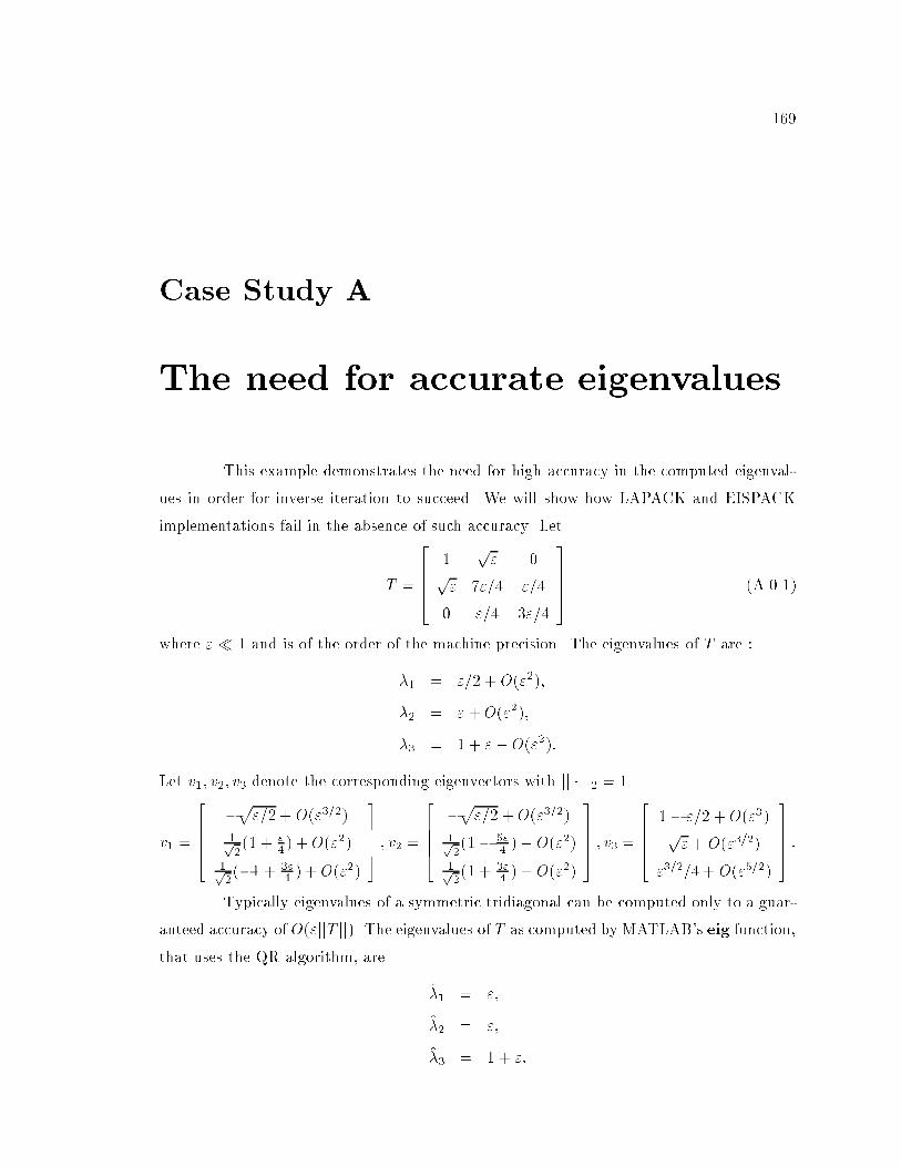
169
Case Study A
The need for accurate eigenvalues
This example demonstrates the need for high accuracy in the computed eigenval-
ues in order for inverse iteration to succeed. We will show how LAPACK and EISPACK
implementations fail in the absence of such accuracy. Let
T =
26664
1p" 0
p" 7"=4 "=4
0 "=4 3"=4
37775 (A.0.1)
where "� 1 and is of the order of the machine precision. The eigenvalues of T are :
�1 = "=2 + O("2);
�2 = " +O("2);
�3 = 1 + "+O("2):
Let v1; v2; v3 denote the corresponding eigenvectors with jj � jj2 = 1.
v1 =
26664
�p"=2 +O("3=2)
1p2(1 + "
4) +O("2)
1p2(�1 + 3"
4) +O("2)
37775 ; v2 =
26664
�p"=2 +O("3=2)
1p2(1� 5"
4) + O("2)
1p2(1 + 3"
4) + O("2)
37775 ; v3 =
26664
1� "=2 +O("3)p"+ O("3=2)
"3=2=4 + O("5=2)
37775 :
Typically eigenvalues of a symmetric tridiagonal can be computed only to a guar-
anteed accuracy of O("jjT jj). The eigenvalues of T as computed by MATLAB's eig function,
that uses the QR algorithm, are
�1 = ";
�2 = ";
�3 = 1 + ":
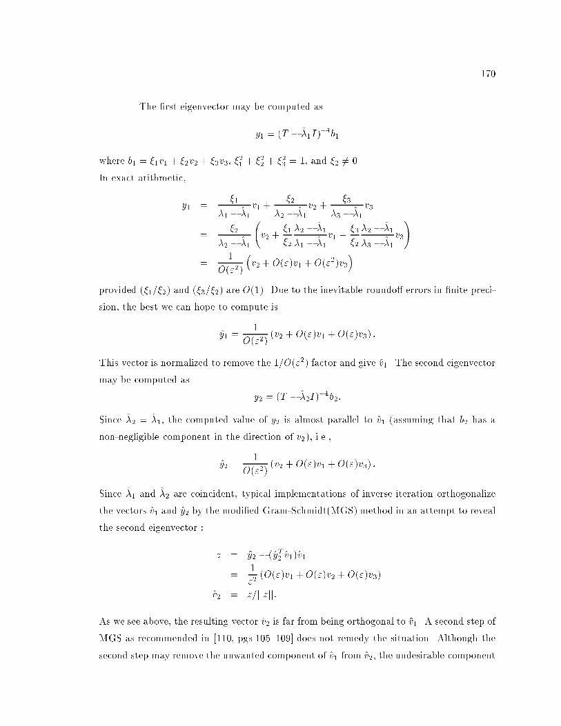
170
The �rst eigenvector may be computed as
y1 = (T � �1I)�1b1
where b1 = �1v1 + �2v2 + �3v3, �21 + �22 + �23 = 1, and �2 6= 0.
In exact arithmetic,
y1 =�1
�1 � �1v1 +
�2
�2 � �1v2 +
�3
�3 � �1v3
=�2
�2 � �1
v2 +
�1
�2
�2 � �1
�1 � �1v1 +
�3
�2
�2 � �1
�3 � �1v3
!
=1
O("2)
�v2 + O(")v1 + O("2)v3
�
provided (�1=�2) and (�3=�2) are O(1). Due to the inevitable roundo� errors in �nite preci-
sion, the best we can hope to compute is
y1 =1
O("2)(v2 + O(")v1 + O(")v3) :
This vector is normalized to remove the 1=O("2) factor and give v1. The second eigenvector
may be computed as
y2 = (T � �2I)�1b2:
Since �2 = �1, the computed value of y2 is almost parallel to v1 (assuming that b2 has a
non-negligible component in the direction of v2), i.e.,
y2 =1
O("2)(v2 + O(")v1 + O(")v3) :
Since �1 and �2 are coincident, typical implementations of inverse iteration orthogonalize
the vectors v1 and y2 by the modi�ed Gram-Schmidt(MGS) method in an attempt to reveal
the second eigenvector :
z = y2 � (yT2 v1)v1
=1
"2(O(")v1 +O(")v2 +O(")v3)
v2 = z=jjzjj:
As we see above, the resulting vector v2 is far from being orthogonal to v1. A second step of
MGS as recommended in [110, pgs.105{109] does not remedy the situation. Although the
second step may remove the unwanted component of v1 from v2, the undesirable component
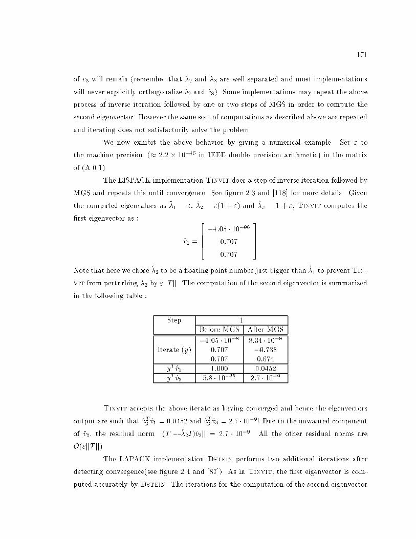
171
of v3 will remain (remember that �2 and �3 are well separated and most implementations
will never explicitly orthogonalize v2 and v3). Some implementations may repeat the above
process of inverse iteration followed by one or two steps of MGS in order to compute the
second eigenvector. However the same sort of computations as described above are repeated
and iterating does not satisfactorily solve the problem.
We now exhibit the above behavior by giving a numerical example. Set " to
the machine precision (� 2:2 � 10�16 in IEEE double precision arithmetic) in the matrix
of (A.0.1).
The EISPACK implementation Tinvit does a step of inverse iteration followed by
MGS and repeats this until convergence. See �gure 2.3 and [118] for more details. Given
the computed eigenvalues as �1 = ", �2 = "(1 + ") and �3 = 1 + ", Tinvit computes the
�rst eigenvector as :
v1 =
26664�1:05 � 10�08
0:707
0:707
37775
Note that here we chose �2 to be a oating point number just bigger than �1 to prevent Tin-
vit from perturbing �2 by "jjT jj. The computation of the second eigenvector is summarized
in the following table :
Step 1
Before MGS After MGS
�1:05 � 10�8 8:34 � 10�9Iterate (y) 0:707 �0:738
0:707 0:674
yT v1 1:000 0:0452
yT v3 5:8 � 10�25 2:7 � 10�9
Tinvit accepts the above iterate as having converged and hence the eigenvectors
output are such that vT2 v1 = 0:0452 and vT2 v3 = 2:7 �10�9! Due to the unwanted component
of v3, the residual norm jj(T � �2I)v2jj = 2:7 � 10�9. All the other residual norms are
O("jjT jj).The LAPACK implementation Dstein performs two additional iterations after
detecting convergence(see �gure 2.4 and [87]). As in Tinvit, the �rst eigenvector is com-
puted accurately by Dstein. The iterations for the computation of the second eigenvector
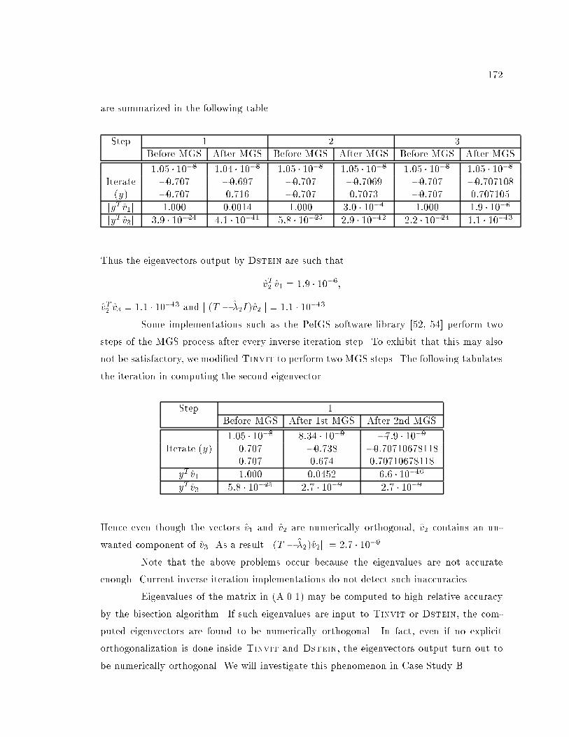
172
are summarized in the following table.
Step 1 2 3
Before MGS After MGS Before MGS After MGS Before MGS After MGS
1:05 � 10�8 1:04 � 10�8 1:05 � 10�8 1:05 � 10�8 1:05 � 10�8 1:05 � 10�8Iterate �0:707 �0:697 �0:707 �0:7069 �0:707 �0:707108(y) �0:707 0:716 �0:707 0:7073 �0:707 0:707105
jyT v1j 1:000 0:0014 1:000 3:0 � 10�4 1:000 1:9 � 10�6jyT v3j 3:9 � 10�24 4:1 � 10�11 5:8 � 10�25 2:9 � 10�12 2:2 � 10�24 1:1 � 10�13
Thus the eigenvectors output by Dstein are such that
vT2 v1 = 1:9 � 10�6;
vT2 v3 = 1:1 � 10�13 and jj(T � �2I)v2jj = 1:1 � 10�13.Some implementations such as the PeIGS software library [52, 54] perform two
steps of the MGS process after every inverse iteration step. To exhibit that this may also
not be satisfactory, we modi�ed Tinvit to perform two MGS steps. The following tabulates
the iteration in computing the second eigenvector.
Step 1
Before MGS After 1st MGS After 2nd MGS
1:05 � 10�8 8:34 � 10�9 �7:9 � 10�9Iterate (y) 0:707 �0:738 �0:70710678118
0:707 0:674 0:70710678118
yT v1 1:000 0:0452 6:6 � 10�16yT v3 5:8 � 10�25 2:7 � 10�9 2:7 � 10�9
Hence even though the vectors v1 and v2 are numerically orthogonal, v2 contains an un-
wanted component of v3. As a result jj(T � �2)v2jj = 2:7 � 10�9.Note that the above problems occur because the eigenvalues are not accurate
enough. Current inverse iteration implementations do not detect such inaccuracies.
Eigenvalues of the matrix in (A.0.1) may be computed to high relative accuracy
by the bisection algorithm. If such eigenvalues are input to Tinvit or Dstein, the com-
puted eigenvectors are found to be numerically orthogonal. In fact, even if no explicit
orthogonalization is done inside Tinvit and Dstein, the eigenvectors output turn out to
be numerically orthogonal. We will investigate this phenomenon in Case Study B.
173
Case Study B
Bidiagonals are Better
The purpose of this case study is to show that a tridiagonal matrix is \better"
represented by a product of bidiagonal matrices for the task of computing eigenvalues and
eigenvectors.
When any numerical algorithm is implemented on a computer, roundo� error needs
to be accounted for, and it is good practice to show that calculations are not destroyed by
the limited precision of the arithmetic operations. Wilkinson made popular the art of
backward error analysis, whereby the computed solution is shown (if possible) to be the
exact solution corresponding to data that is slightly di�erent from the input data [135].
When combined with knowledge about the sensitivity of the solution to small changes in
the data, this approach enables us to prove the accuracy of various numerical procedures.
A real, symmetric tridiagonal matrix T is traditionally represented by its n di-
agonal and n � 1 o�-diagonal elements. Some highly accurate algorithms for �nding the
eigenvalues of T , such as bisection, can be shown to �nd an exact eigenpair of T +�T , where
the perturbation �T is a small relative perturbation in only the o�-diagonals of T . In this
Case Study, by examining the e�ect of such perturbations on the spectrum of T , we show
that for our purposes it is better to represent a tridiagonal matrix by its bidiagonal factors.
First, we examine the matrix we encountered in Case Study A earlier, and observe
that it does have the perturbation properties we desire. However not all tridiagonals share
this property and we will illustrate this with another matrix.
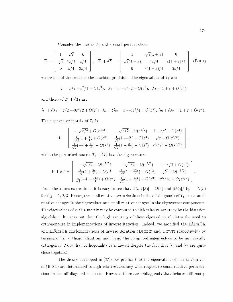
174
Consider the matrix T1 and a small perturbation :
T1 =
26664
1p" 0
p" 7"=4 "=4
0 "=4 3"=4
37775 ; T1 + �T1 =
26664
1p"(1 + ") 0
p"(1 + ") 7"=4 "(1 + ")=4
0 "(1 + ")=4 3"=4
37775 (B.0.1)
where " is of the order of the machine precision. The eigenvalues of T1 are
�1 = "=2� "2=4 + O("3); �2 = " � "2=2 + O("3); �3 = 1 + "+O("2);
and those of T1 + �T1 are
�1 + ��1 = "=2� 3"2=2 +O("3); �2 + ��2 = "� 5"2=4 +O("3); �3 + ��3 = 1 + " +O("2):
The eigenvector matrix of T1 is
V =
26664
�p"=2 +O("3=2) �p"=2 + O("3=2) 1� "=2 +O("2)
1p2(1 + "
4) +O("2) 1p
2(1� 5"
4) + O("2)
p"+ O("3=2)
1p2(�1 + 3"
4) +O("2) 1p
2(1 + 3"
4) + O("2) "3=2=4 + O("5=2)
37775 ;
while the perturbed matrix T1 + �T1 has the eigenvectors
V + �V =
26664
�p"=2 + O("3=2) �p"=2 + O("3=2) 1� "=2 + O("2)
1p2(1 + 9"
4) + O("2) 1p
2(1� 13"
4) + O("2)
p"+O("3=2)
1p2(�1 + 11"
4) +O("2) 1p
2(1 + 11"
4) + O("2) "3=2=4 + O("5=2)
37775 :
From the above expressions, it is easy to see that j��jj=j�jj = O(") and j�Vijj=jVijj = O(")
for i; j = 1; 2; 3. Hence, the small relative perturbations in the o�-diagonals of T1 cause small
relative changes in the eigenvalues and small relative changes in the eigenvector components.
The eigenvalues of such a matrix may be computed to high relative accuracy by the bisection
algorithm. It turns out that the high accuracy of these eigenvalues obviates the need to
orthogonalize in implementations of inverse iteration. Indeed, we modi�ed the LAPACK
and EISPACK implementations of inverse iteration (Dstein and Tinvit respectively) by
turning o� all orthogonalization, and found the computed eigenvectors to be numerically
orthogonal. Note that orthogonality is achieved despite the fact that �1 and �2 are quite
close together!
The theory developed in [37] does predict that the eigenvalues of matrix T1 given
in (B.0.1) are determined to high relative accuracy with respect to small relative perturba-
tions in the o�-diagonal elements. However there are tridiagonals that behave di�erently.
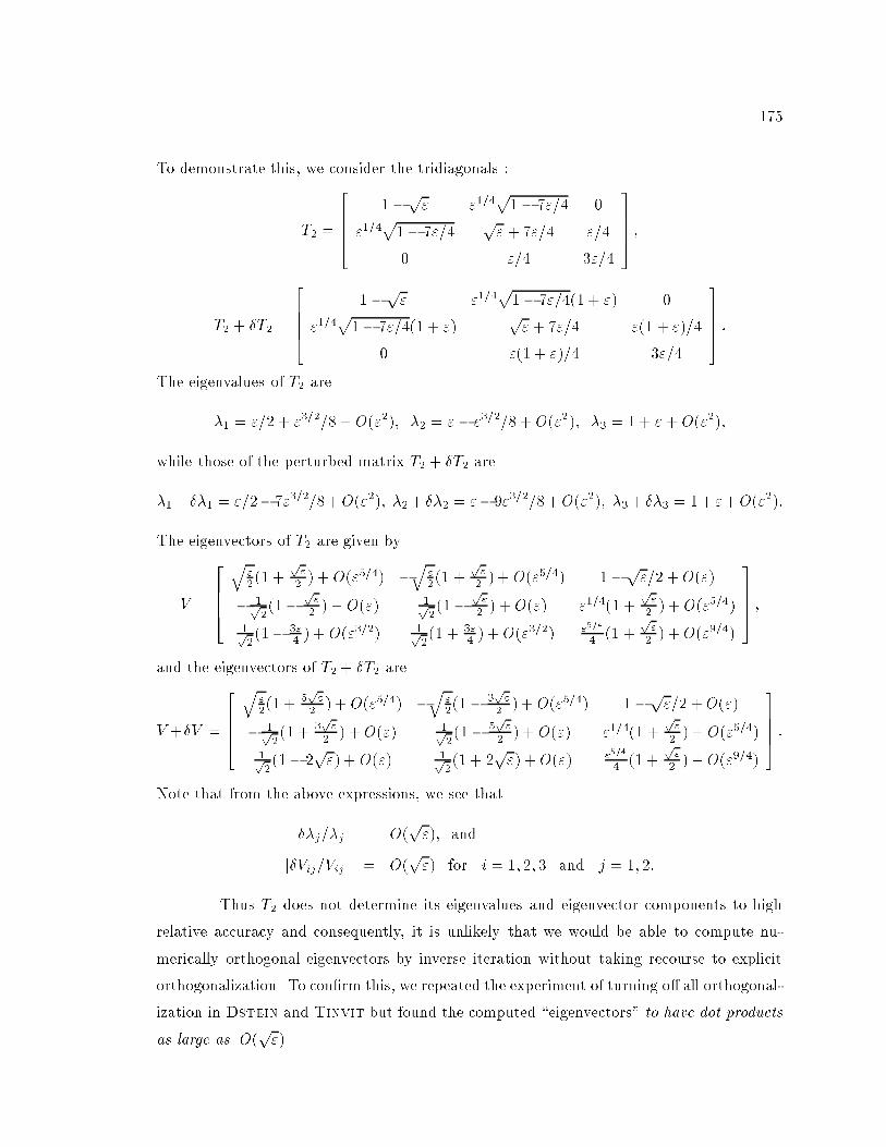
175
To demonstrate this, we consider the tridiagonals :
T2 =
26664
1�p" "1=4p1� 7"=4 0
"1=4p1� 7"=4
p" + 7"=4 "=4
0 "=4 3"=4
37775 ;
T2 + �T2 =
26664
1�p" "1=4p1� 7"=4(1 + ") 0
"1=4p1� 7"=4(1 + ")
p" + 7"=4 "(1 + ")=4
0 "(1 + ")=4 3"=4
37775 :
The eigenvalues of T2 are
�1 = "=2 + "3=2=8 + O("2); �2 = " � "3=2=8 +O("2); �3 = 1+ "+ O("2);
while those of the perturbed matrix T2 + �T2 are
�1+ ��1 = "=2� 7"3=2=8+O("2); �2+ ��2 = "� 9"3=2=8+O("2); �3+ ��3 = 1+ "+O("2):
The eigenvectors of T2 are given by
V =
26664q
"2(1 +
p"2) + O("5=4) �
q"2(1 +
p"2) + O("5=4) 1�p"=2 +O(")
� 1p2(1�
p"2) + O(") 1p
2(1�
p"2) + O(") "1=4(1 +
p"2) + O("5=4)
1p2(1� 3"
4) + O("3=2) 1p
2(1 + 3"
4) +O("3=2) "5=4
4(1 +
p"2) +O("9=4)
37775 ;
and the eigenvectors of T2 + �T2 are
V +�V =
26664q
"2(1 + 5
p"
2) + O("5=4) �
q"2(1� 3
p"
2) + O("5=4) 1�p"=2 +O(")
� 1p2(1 +
3p"
2) +O(") 1p
2(1� 5
p"
2) + O(") "1=4(1 +
p"2) + O("5=4)
1p2(1� 2
p") + O(") 1p
2(1 + 2
p") + O(") "5=4
4(1 +
p"2) +O("9=4)
37775 :
Note that from the above expressions, we see that
j��j=�jj = O(p"); and
j�Vij=Vijj = O(p") for i = 1; 2; 3 and j = 1; 2:
Thus T2 does not determine its eigenvalues and eigenvector components to high
relative accuracy and consequently, it is unlikely that we would be able to compute nu-
merically orthogonal eigenvectors by inverse iteration without taking recourse to explicit
orthogonalization. To con�rm this, we repeated the experiment of turning o� all orthogonal-
ization in Dstein and Tinvit but found the computed \eigenvectors" to have dot products
as large as O(p").
176
However, there is a way out of this impasse. Since T2 is positive de�nite, we can
form its Cholesky decomposition,
T2 = LLT :
Due to the tridiagonal form of T2, the Cholesky factor L is bidiagonal. It is now known
that small relative changes to the entries of a bidiagonal matrix cause small relative changes
to its singular values, and small changes in the directions of the singular vectors if the
relative gaps between the singular values are large. Note that the eigenvalues of T2 are the
squares of the singular values of L while its eigenvectors are the left singular vectors of L.
This property of bidiagonal matrices gives us an impetus to produce algorithms where the
backward errors may be posed as small relative changes in L rather than in T . By doing
so we can eliminate the need for orthogonalization when �nding eigenvectors of T2 since its
eigenvalues are relatively far apart. We have accomplished this task in Chapter 4.
The observant reader will notice that both T1 and T2 are positive de�nite and thus
admit Cholesky decomposition. What can we do if the tridiagonal is inde�nite? In such
a case, we could turn to the LU decomposition of the tridiagonal. However, the relative
perturbation theory in the inde�nite case has not been extensively studied and is not well
understood. We attempt to answer some questions in Chapter 5.
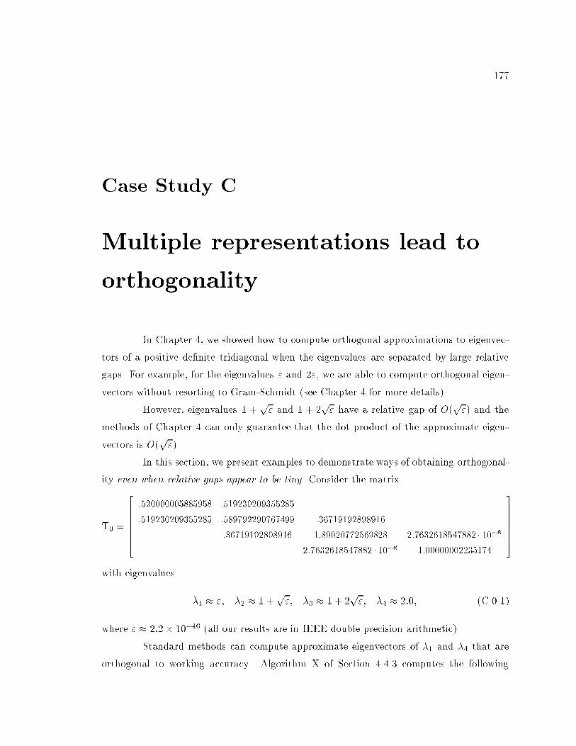
177
Case Study C
Multiple representations lead to
orthogonality
In Chapter 4, we showed how to compute orthogonal approximations to eigenvec-
tors of a positive de�nite tridiagonal when the eigenvalues are separated by large relative
gaps. For example, for the eigenvalues " and 2", we are able to compute orthogonal eigen-
vectors without resorting to Gram-Schmidt (see Chapter 4 for more details).
However, eigenvalues 1 +p" and 1 + 2
p" have a relative gap of O(
p") and the
methods of Chapter 4 can only guarantee that the dot product of the approximate eigen-
vectors is O(p").
In this section, we present examples to demonstrate ways of obtaining orthogonal-
ity even when relative gaps appear to be tiny. Consider the matrix
T0 =
2666664:520000005885958 :519230209355285
:519230209355285 :589792290767499 :36719192898916
:36719192898916 1:89020772569828 2:7632618547882 � 10�8
2:7632618547882 � 10�8 1:00000002235174
3777775
with eigenvalues
�1 � "; �2 � 1 +p"; �3 � 1 + 2
p"; �4 � 2:0; (C.0.1)
where " � 2:2� 10�16 (all our results are in IEEE double precision arithmetic).
Standard methods can compute approximate eigenvectors of �1 and �4 that are
orthogonal to working accuracy. Algorithm X of Section 4.4.3 computes the following
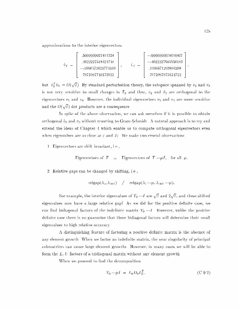
178
approximations to the interior eigenvectors
v2 =
2666664
:5000000027411224
:4622227318424748
�:1906571623774349
:7071067740172921
3777775 ; v3 =
2666664
�:5000000074616407
�:4622227505556183
:1906571293895208
:7071067673414712
3777775 ;
but jvT2 v3j = O(p"). By standard perturbation theory, the subspace spanned by v2 and v3
is not very sensitive to small changes in T0 and thus, v2 and v3 are orthogonal to the
eigenvectors v1 and v4. However, the individual eigenvectors v2 and v3 are more sensitive
and the O(p") dot products are a consequence.
In spite of the above observation, we can ask ourselves if it is possible to obtain
orthogonal v2 and v3 without resorting to Gram-Schmidt. A natural approach is to try and
extend the ideas of Chapter 4 which enable us to compute orthogonal eigenvectors even
when eigenvalues are as close as " and 2". We make two crucial observations
1. Eigenvectors are shift invariant, i.e.,
Eigenvectors of T � Eigenvectors of T � �I; for all �:
2. Relative gaps can be changed by shifting, i.e.,
relgap(�i; �i+1) 6= relgap(�i � �; �i+1 � �):
For example, the interior eigenvalues of T0� I arep" and 2
p", and these shifted
eigenvalues now have a large relative gap! As we did for the positive de�nite case, we
can �nd bidiagonal factors of the inde�nite matrix T0 � I . However, unlike the positive
de�nite case there is no guarantee that these bidiagonal factors will determine their small
eigenvalues to high relative accuracy.
A distinguishing feature of factoring a positive de�nite matrix is the absence of
any element growth. When we factor an inde�nite matrix, the near singularity of principal
submatrices can cause large element growths. However, in many cases we will be able to
form the L, U factors of a tridiagonal matrix without any element growth.
When we proceed to �nd the decomposition
T0 � �I = L0D0LT0 ; (C.0.2)
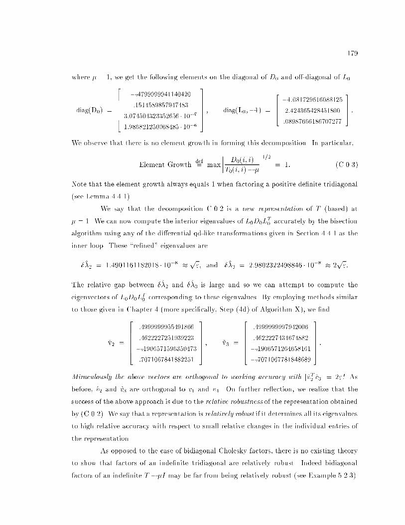
179
where � = 1, we get the following elements on the diagonal of D0 and o�-diagonal of L0.
diag(D0) =
2666664
�:4799999941140420
:1514589857947483
3:074504323352656 � 10�7
1:986821250068485 � 10�8
3777775 ; diag(L0;�1) =
2664
�1:081729616088125
2:424365428451800
:08987666186707277
3775 :
We observe that there is no element growth in forming this decomposition. In particular,
Element Growthdef= max
���� D0(i; i)
T0(i; i)� �
����1=2
= 1: (C.0.3)
Note that the element growth always equals 1 when factoring a positive de�nite tridiagonal
(see Lemma 4.4.1).
We say that the decomposition C.0.2 is a new representation of T (based) at
� = 1. We can now compute the interior eigenvalues of L0D0LT0 accurately by the bisection
algorithm using any of the di�erential qd-like transformations given in Section 4.4.1 as the
inner loop. These \re�ned" eigenvalues are
��2 = 1:4901161182018 � 10�8 � p"; and ��3 = 2:9802322498846 � 10�8 � 2
p":
The relative gap between ��2 and ��3 is large and so we can attempt to compute the
eigenvectors of L0D0LT0 corresponding to these eigenvalues. By employing methods similar
to those given in Chapter 4 (more speci�cally, Step (4d) of Algorithm X), we �nd
v2 =
2666664
:4999999955491866
:4622227251939223
�:1906571596350473
:7071067841882251
3777775 ; v3 =
2666664
:4999999997942006
:4622227434674882
�:1906571264658161
�:7071067781848689
3777775 :
Miraculously the above vectors are orthogonal to working accuracy with jvT2 v3j = 2"! As
before, v2 and v3 are orthogonal to v1 and v4. On further re ection, we realize that the
success of the above approach is due to the relative robustness of the representation obtained
by (C.0.2). We say that a representation is relatively robust if it determines all its eigenvalues
to high relative accuracy with respect to small relative changes in the individual entries of
the representation.
As opposed to the case of bidiagonal Cholesky factors, there is no existing theory
to show that factors of an inde�nite tridiagonal are relatively robust. Indeed bidiagonal
factors of an inde�nite T ��I may be far from being relatively robust (see Example 5.2.3).
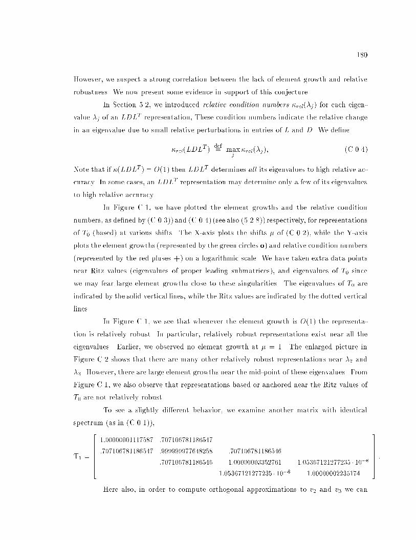
180
However, we suspect a strong correlation between the lack of element growth and relative
robustness. We now present some evidence in support of this conjecture.
In Section 5.2, we introduced relative condition numbers �rel(�j) for each eigen-
value �j of an LDLT representation, These condition numbers indicate the relative change
in an eigenvalue due to small relative perturbations in entries of L and D. We de�ne
�rel(LDLT )def= max
j�rel(�j); (C.0.4)
Note that if �(LDLT ) = O(1) then LDLT determines all its eigenvalues to high relative ac-
curacy. In some cases, an LDLT representation may determine only a few of its eigenvalues
to high relative accuracy.
In Figure C.1, we have plotted the element growths and the relative condition
numbers, as de�ned by (C.0.3)) and (C.0.4) (see also (5.2.8)) respectively, for representations
of T0 (based) at various shifts. The X-axis plots the shifts � of (C.0.2), while the Y-axis
plots the element growths (represented by the green circles o) and relative condition numbers
(represented by the red pluses +) on a logarithmic scale. We have taken extra data points
near Ritz values (eigenvalues of proper leading submatrices), and eigenvalues of T0 since
we may fear large element growths close to these singularities. The eigenvalues of T0 are
indicated by the solid vertical lines, while the Ritz values are indicated by the dotted vertical
lines.
In Figure C.1, we see that whenever the element growth is O(1) the representa-
tion is relatively robust. In particular, relatively robust representations exist near all the
eigenvalues. Earlier, we observed no element growth at � = 1. The enlarged picture in
Figure C.2 shows that there are many other relatively robust representations near �2 and
�3. However, there are large element growths near the mid-point of these eigenvalues. From
Figure C.1, we also observe that representations based or anchored near the Ritz values of
T0 are not relatively robust.
To see a slightly di�erent behavior, we examine another matrix with identical
spectrum (as in (C.0.1)),
T1 =
2666664
1:00000001117587 :707106781186547
:707106781186547 :999999977648258 :707106781186546
:707106781186546 1:00000003352761 1:05367121277235 � 10�8
1:05367121277235 � 10�8 1:00000002235174
3777775 :
Here also, in order to compute orthogonal approximations to v2 and v3 we can
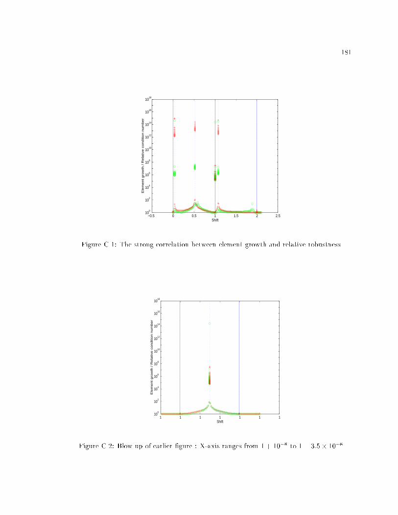
181
−0.5 0 0.5 1 1.5 2 2.510
0
102
104
106
108
1010
1012
1014
1016
1018
Shift
Ele
me
nt g
row
th / R
ela
tive
co
nd
itio
n n
um
be
r
Figure C.1: The strong correlation between element growth and relative robustness
1 1 1 1 1 1 110
0
102
104
106
108
1010
1012
1014
1016
1018
Shift
Ele
me
nt g
row
th / R
ela
tive
co
nd
itio
n n
um
be
r
Figure C.2: Blow up of earlier �gure : X-axis ranges from 1+ 10�8 to 1 + 3:5� 10�8
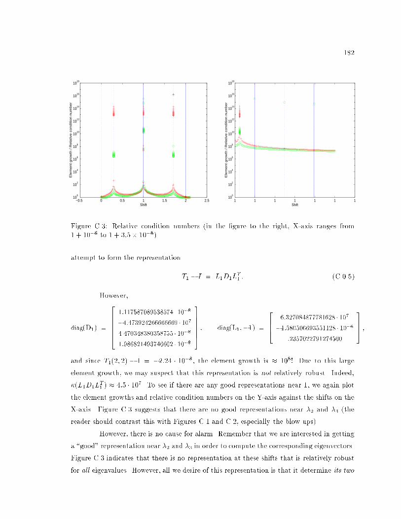
182
−0.5 0 0.5 1 1.5 2 2.510
0
102
104
106
108
1010
1012
1014
1016
1018
Shift
Ele
me
nt g
row
th / R
ela
tive
co
nd
itio
n n
um
be
r
1 1 1 1 1 1 110
0
102
104
106
108
1010
1012
1014
1016
1018
Shift
Ele
me
nt g
row
th / R
ela
tive
co
nd
itio
n n
um
be
rFigure C.3: Relative condition numbers (in the �gure to the right, X-axis ranges from
1 + 10�8 to 1 + 3:5� 10�8)
attempt to form the representation
T1 � I = L1D1LT1 : (C.0.5)
However,
diag(D1) =
2666664
1:117587089538574 � 10�8
�4:473924266666669 � 107
4:470348380358755 � 10�8
1:986821493746602 � 10�8
3777775 ; diag(L1;�1) =
2664
6:327084877781628 � 107
�1:580506693551128 � 10�8
:2357022791274500
3775 ;
and since T1(2; 2) � 1 = �2:24 � 10�8, the element growth is � 108! Due to this large
element growth, we may suspect that this representation is not relatively robust. Indeed,
�(L1D1LT1 ) � 4:5 � 107. To see if there are any good representations near 1, we again plot
the element growths and relative condition numbers on the Y-axis against the shifts on the
X-axis. Figure C.3 suggests that there are no good representations near �2 and �3 (the
reader should contrast this with Figures C.1 and C.2, especially the blow ups).
However, there is no cause for alarm. Remember that we are interested in getting
a \good" representation near �2 and �3 in order to compute the corresponding eigenvectors.
Figure C.3 indicates that there is no representation at these shifts that is relatively robust
for all eigenvalues. However, all we desire of this representation is that it determine its two
183
smallest eigenvalues to high relative accuracy. Indeed, we discover that despite the large
element growths, the relative condition numbers �rel(�2) and �rel(�3) for the representations
close to �2 and �3 are O(1), i.e., the representations near 1 do determine their two smallest
eigenvalues to high relative accuracy. Thus, just as before, we can compute v2 and v3 from
the representation based at 1, and get
v2 =
2666664
:4999999981373546
2:634178061370114 � 10�9
�:4999999981373549
:7071067838207259
3777775 ; v3 =
2666664
�:5000000018626457
�1:317089024797209 � 10�8
:5000000018626453
:7071067785523688
3777775 ; (C.0.6)
where jvT2 v3j < 3"!
We have observed numerical behavior similar to T0 and T1 in many larger matrices.
The more common case shows no element growth for shifts near the eigenvalues, whereas
large element growths, as in the case of T1, occur rarely. The study of relative condition
numbers of individual eigenvalues, especially the tiny ones, is pursued in Chapter 5.