Embed Size (px)
Citation preview
Copyright © by SIAM. Unauthorized reproduction of this article is prohibited.
SIAM J. MATRIX ANAL. APPL. c© 2007 Society for Industrial and Applied MathematicsVol. 29, No. 4, pp. 1120–1146
MATRIX NEARNESS PROBLEMS WITH BREGMANDIVERGENCES∗
INDERJIT S. DHILLON† AND JOEL A. TROPP‡
Abstract. This paper discusses a new class of matrix nearness problems that measure approx-imation error using a directed distance measure called a Bregman divergence. Bregman divergencesoffer an important generalization of the squared Frobenius norm and relative entropy, and they allshare fundamental geometric properties. In addition, these divergences are intimately connectedwith exponential families of probability distributions. Therefore, it is natural to study matrix ap-proximation problems with respect to Bregman divergences. This article proposes a framework forstudying these problems, discusses some specific matrix nearness problems, and provides algorithmsfor solving them numerically. These algorithms apply to many classical and novel problems, andthey admit a striking geometric interpretation.
Key words. matrix nearness problems, Bregman divergences, squared Euclidean distance,relative entropy, alternating projections
AMS subject classifications. 15A99, 65F30, 90C25
DOI. 10.1137/060649021
1. Introduction. A recurring problem in matrix theory is to find a structuredmatrix that best approximates a given matrix with respect to some distance measure.For example, it may be known a priori that a certain constraint ought to hold, andyet it fails on account of measurement errors or numerical roundoff. An attractiveremedy is to replace the tainted matrix by the nearest matrix that does satisfy theconstraint. Matrix approximation problems typically measure the distance betweenmatrices with a norm. The Frobenius and spectral norms are pervasive choices becausethey are so analytically tractable. Nevertheless, these norms are not always defensiblein applications, where it may be wiser to tailor the distance measure to the context.
In this paper, we discuss a new class of matrix nearness problems that use adirected distance measure called a Bregman divergence. Given a differentiable, strictlyconvex function ϕ that maps matrices to the extended real numbers, we define theBregman divergence of the matrix X from the matrix Y as
Dϕ(X;Y )def= ϕ(X) − ϕ(Y ) − 〈∇ϕ(Y ),X − Y 〉 ,
where the inner product 〈X,Y 〉 = Re TrXY ∗. The two principal examples of Breg-man divergences deserve immediate mention. When ϕ(X) = 1
2‖X‖2F , the associated
divergence is the squared Frobenius norm 12‖X − Y ‖2
F . When ϕ is the negativeShannon entropy, we obtain the Kullback–Leibler divergence, which is also known asrelative entropy. But these two cases are just the tip of the iceberg.
Bregman divergences are well suited for nearness problems because they sharemany geometric properties with the squared Frobenius norm. They also exhibit an
∗Received by the editors January 4, 2006; accepted for publication (in revised form) by N. J.Higham March 20, 2007; published electronically November 21, 2007.
http://www.siam.org/journals/simax/29-4/64902.html†Department of Computer Sciences, University of Texas, Austin, TX 78712-1188 (inderjit@
cs.utexas.edu). This author’s research was supported by NSF grant CCF-0431257, NSF career awardACI-0093404, and NSF-ITR award IIS-0325116.
‡Applied and Computational Mathematics, California Institute of Technology, Pasadena, CA91125-5000 ([email protected]). This author’s research was supported by an NSF graduatefellowship.
1120
Copyright © by SIAM. Unauthorized reproduction of this article is prohibited.
MATRIX NEARNESS WITH BREGMAN DIVERGENCES 1121
intimate relationship with exponential families of probability distributions, which rec-ommends them for solving problems that arise in the statistical analysis of data. Wewill elaborate on these connections in what follows.
Let us begin with a formal statement of the Bregman nearness problem. Supposethat Dϕ is a Bregman divergence, and suppose that {Ck} is a finite collection ofclosed, convex sets whose intersection is nonempty. Given an input matrix Y , ourgoal is to produce a matrix X in the intersection that diverges the least from Y , i.e.,to solve
(1.1) minX
Dϕ(X;Y ) subject to X ∈⋂
kCk.
Under mild conditions, the solution to (1.1) is unique, and it has a variational char-acterization analogous with the characterization of an orthogonal projection onto aconvex set [10]. Minimization with respect to the second argument of the divergenceenjoys rather less structure, so we refer the reader to [5] for more details. A majoradvantage of our problem formulation is that it admits a natural algorithm. If onepossesses a method for minimizing the divergence over each of the constraint sets,then it is possible to solve (1.1) by minimizing over each constraint in turn while in-troducing a series of simple corrections. Several classical algorithms from the matrixliterature fit into this geometric framework, but it also provides an approach to manynovel problems.
We view this paper as an expository work with two central goals. First, it in-troduces Bregman divergences to the matrix theory literature, and it argues thatthey provide an important and natural class of distance measures for matrix nearnessproblems. Moreover, the article unifies a large class of problems into a geometricalframework, and it shows that these problems can be solved with a set of classicalalgorithms. Second, the paper provides specific examples of nearness problems withrespect to Bregman divergences. One example is the familiar problem of producingthe nearest contingency table with fixed marginals. Novel examples include comput-ing matrix approximations using the minimum Bregman information (MBI) principle,identifying the metric graph nearest to an arbitrary graph, and determining the near-est correlation and kernel matrix with respect to matrix divergences, such as the vonNeumann divergence. These applications show how Bregman divergences can be usedto preserve and exploit additional structure that appears in a problem.
We must warn the reader that, in spite of the availability of some general purposealgorithms for working with Bregman divergences, they may require a substantialamount of computational effort. One basic reason is that nearness problems withrespect to the Frobenius norm usually remain within the domain of linear algebra,which is a developed technology. Bregman divergences, on the other hand, transportus to the world of convex optimization, which is a rougher frontier. As outlined insection 8, there remain many unresolved research issues on the computational aspectsof Bregman divergences.
Here is a brief outline of the article. Section 2 introduces Bregman divergences andBregman projections along with their connection to exponential families of probabilitydistributions. Matrix Bregman divergences that depend on the spectral propertiesof a matrix are covered in subsection 2.6. Section 3 discusses numerical methodsfor the basic problem of minimizing a Bregman divergence over a hyperplane. Insection 4, we develop the successive projection algorithm for solving the Bregmannearness problem subject to affine constraints. Section 5 gives several examples ofthese problems: finding the nearest contingency table with fixed marginals, computing
Copyright © by SIAM. Unauthorized reproduction of this article is prohibited.
1122 INDERJIT S. DHILLON AND JOEL A. TROPP
matrix approximations for data analysis, and determining the nearest correlationmatrix with respect to the von Neumann divergence. Section 6 presents the successiveprojection–correction algorithm for solving the Bregman nearness problem subject toa polyhedral constraint. In section 7 we discuss two matrix nearness problems withnonaffine constraints: finding the nearest metric graph and learning a kernel matrixfor data mining and machine learning applications.
2. Bregman divergences and Bregman projections. This section developsthe directed distance functions that were first studied by Bregman [8]. Our primarysource is the superb article of Bauschke and Borwein [4], which studies a subclassof Bregman divergences that exhibits many desirable properties in connection withnearness problems like (1.1).
2.1. Convex analysis. The literature on Bregman divergences involves a sig-nificant amount of convex analysis. Some standard references for this material are[35, 20]. We review some of these ideas in an effort to make this article accessible toreaders who are less familiar with this field.
We will work in a finite-dimensional, real inner-product space X . The real-linearinner product is denoted by 〈·, ·〉 and the induced norm by ‖·‖2. In general, theelements of X will be expressed with lowercase bold italic letters such as x and y.We will switch to capitals, such as X and Y , when it is important to view the elementsof X as matrices.
A convex set is a subset C of X that exhibits the property
sx + (1 − s)y ∈ C for all s ∈ (0, 1) and x,y ∈ C.
In words, the line segment connecting each pair of points in a convex set falls withinthe set. The relative interior of a convex set, abbreviated ri, is the interior of thatset considered as a subset of the lowest-dimensional affine space that contains it.
In convex analysis, functions are defined on all of X , and they take values in theextended real numbers, R ∪ {±∞}. The (effective) domain of a function f is the set
dom fdef= {x ∈ X : f(x) < +∞}.
A function f is convex if its domain is convex and it verifies the inequality
f(sx + (1 − s)y) ≤ s f(x) + (1 − s) f(y) for all s ∈ (0, 1) and x,y ∈ dom f .
If the inequality is strict, then f is strictly convex. In words, the chord connectingeach pair of points on the graph of a (strictly) convex function lies (strictly) above thegraph. A convex function is proper if it takes at least one finite value and never takesthe value −∞. A convex function f is closed if its lower level set {x : f(x) ≤ α} isclosed for each real α. In particular, a convex function is closed whenever its domainis closed (but not conversely).
For completeness, we also introduce some technical definitions that the casualreader may prefer to glide through. A proper convex function f is called essentiallysmooth if it is everywhere differentiable on the (nonempty) interior of its domain andif ‖∇f(xt)‖ tends to infinity for every sequence {xt} from ri(dom f) that converges toa point on the boundary of dom f . Roughly speaking, an essentially smooth functioncannot be extended to a convex function with a larger domain. The function f(x) =− log(x) with domain (0,+∞) is an example of an essentially smooth function. Inwhat follows, we will focus on convex functions of Legendre type. A Legendre function
Copyright © by SIAM. Unauthorized reproduction of this article is prohibited.
MATRIX NEARNESS WITH BREGMAN DIVERGENCES 1123
is a closed, proper, convex function that is essentially smooth and also strictly convexon the relative interior of its domain.
Every convex function has a dual representation in terms of its supporting hyper-planes. This idea is formalized in the Fenchel conjugate, which is defined as
f∗(θ)def= supx
{〈x,θ〉 − f(x)
}.
No confusion should arise from our usage of the symbol ∗ for complex-conjugatetransposition as well as Fenchel conjugation. The following facts are valuable. Theconjugate of a convex function is always closed and convex. If f is a closed, convexfunction, then (f∗)∗ = f . A convex function has Legendre type if and only if itsconjugate has Legendre type.
Finally, we say that a convex function f is cofinite when
limξ→∞
f(ξ x)/ξ = +∞ for all nonzero x in X .
This definition means that a cofinite function grows superlinearly in every direction.For example, the function ‖·‖2
2 is cofinite, but the function exp(·) is not. It can beshown that a closed, proper, convex function f is cofinite if and only if dom f∗ = X .
2.2. Divergences. Suppose that ϕ is a convex function of Legendre type. Fromevery such seed function, we may construct a Bregman divergence1
Dϕ : domϕ× ri(domϕ) → [0,+∞)
via the rule
Dϕ(x;y)def= ϕ(x) − ϕ(y) − 〈∇ϕ(y),x− y〉 .
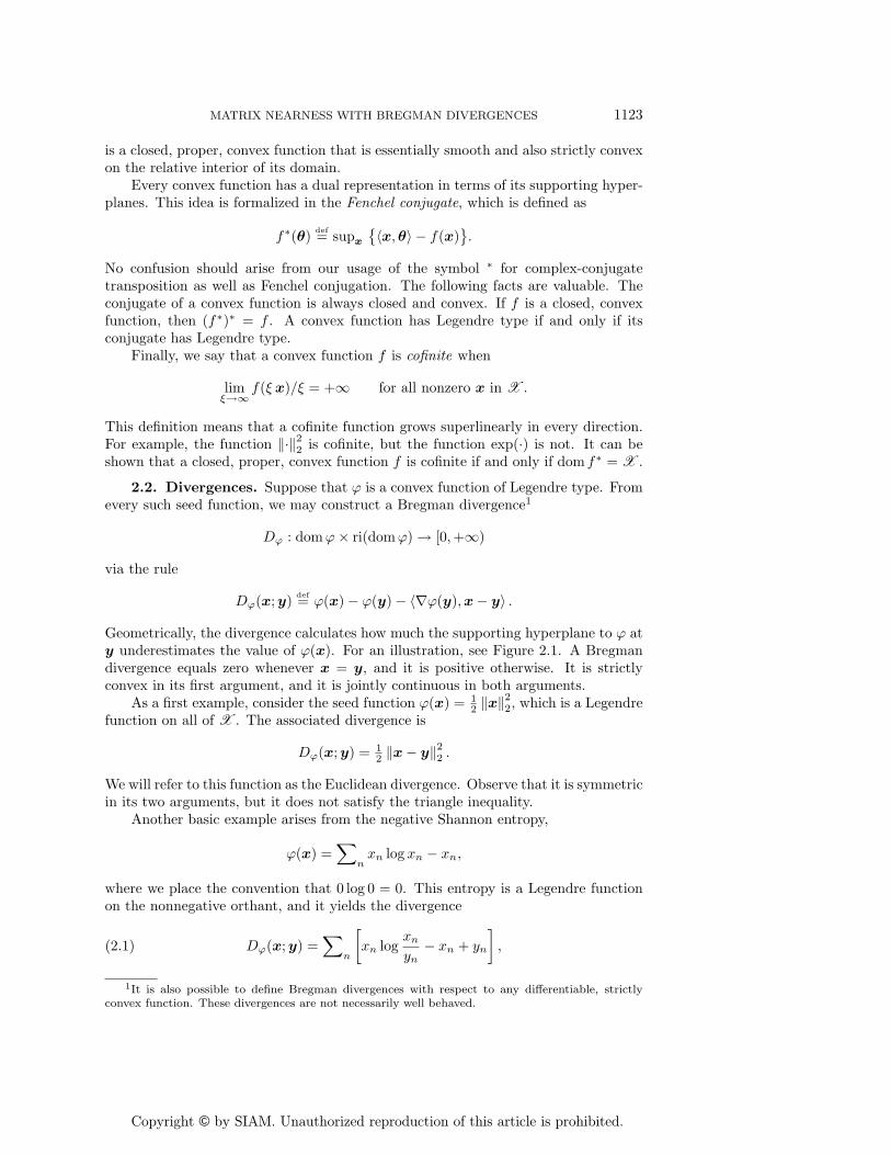
Geometrically, the divergence calculates how much the supporting hyperplane to ϕ aty underestimates the value of ϕ(x). For an illustration, see Figure 2.1. A Bregmandivergence equals zero whenever x = y, and it is positive otherwise. It is strictlyconvex in its first argument, and it is jointly continuous in both arguments.
As a first example, consider the seed function ϕ(x) = 12 ‖x‖
22, which is a Legendre
function on all of X . The associated divergence is
Dϕ(x;y) = 12 ‖x− y‖2
2 .
We will refer to this function as the Euclidean divergence. Observe that it is symmetricin its two arguments, but it does not satisfy the triangle inequality.
Another basic example arises from the negative Shannon entropy,
ϕ(x) =∑
nxn log xn − xn,
where we place the convention that 0 log 0 = 0. This entropy is a Legendre functionon the nonnegative orthant, and it yields the divergence
(2.1) Dϕ(x;y) =∑
n
[xn log
xn
yn− xn + yn
],
1It is also possible to define Bregman divergences with respect to any differentiable, strictlyconvex function. These divergences are not necessarily well behaved.
Copyright © by SIAM. Unauthorized reproduction of this article is prohibited.
1124 INDERJIT S. DHILLON AND JOEL A. TROPP
y x
ϕ(z)= 12 zT z
h(z)
Dϕ(x,y)= 12‖x−y‖2
Fig. 2.1. An example of a Bregman divergence is the squared Euclidean distance. The Bregmandivergence Dϕ(x; y) calculates how much the supporting hyperplane to ϕ at y underestimates thevalue of ϕ(x).
which is variously called the relative entropy, the information divergence, or the gen-eralized Kullback–Leibler divergence. This divergence is not symmetric, and it doesnot satisfy the triangle inequality.
Bregman divergences are often referred to as Bregman distances, but this termi-nology is misleading. A Bregman divergence should not be viewed as a generalizationof a metric but rather as a generalization of the preceding two examples. Like a met-ric, every Bregman divergence is positive except when its arguments coincide. On theother hand, divergences do not generally satisfy the triangle inequality, and they aresymmetric only when the seed function ϕ is quadratic. In compensation, divergencesexhibit other structural properties. For every three points in the interior of domϕ,we have the relation
Dϕ(x;z) = Dϕ(x;y) + Dϕ(y;z) − 〈∇ϕ(z) −∇ϕ(y),x− y〉 .
When Dϕ is the Euclidean divergence, one may identify this formula as the law ofcosines. Later, we will also encounter a Pythagorean theorem.
We also note another expression for the divergence, which emphasizes that it is asort of locally quadratic distance measure,
Dϕ(x;y) = (x− y)∗{∇2ϕ(ξ)
}(x− y),
where ξ is an unknown vector that depends on x and y. This formula can be obtainedfrom the Taylor expansion of the seed function with an exact remainder term.
2.3. Exponential families. Suppose that ψ is a Legendre function. A (full)regular exponential family is a parameterized family of probability distributions onX with density function (with respect to the Lebesgue measure on X ) of the form
pψ(x |θ) = exp{〈x,θ〉 − ψ(θ) − h(x)},
where the parameter θ is drawn from the open set domψ [3]. The function ψ is calledthe cumulant function of the exponential family, and it completely determines thefunction h. The expectation of the distribution pψ( · |θ) is the vector
μ(θ)def=
∫X
x pψ(x |θ) dx,
Copyright © by SIAM. Unauthorized reproduction of this article is prohibited.
MATRIX NEARNESS WITH BREGMAN DIVERGENCES 1125
where dx denotes the Lebesgue measure on X . Many common probability distribu-tions belong to exponential families. Prominent examples include Gaussian, Poisson,Bernoulli, and gamma distributions.
It has recently been established that there is a unique Bregman divergence thatcorresponds to every regular exponential family.
Theorem 1 (Banerjee et al. [2]). Suppose that ϕ and ψ are conjugate Legendrefunctions. Let Dϕ be the Bregman divergence associated with ϕ, and let pψ( · |θ) be amember of the regular exponential family with cumulant function ψ. Then
pψ(x |θ) = exp{−Dϕ(x;μ(θ))} gϕ(x),
where gϕ is a function uniquely determined by ϕ.The spherical Gaussian distribution provides an especially interesting example of
this relationship [2]. Suppose that μ is an arbitrary vector in X , and let σ2 be a fixedpositive number. The spherical Gaussian distributions with mean μ and varianceσ2 form an exponential family with parameter θ = μ/σ2 and cumulant function
ψ(θ) = σ2
2 ‖θ‖22. The Fenchel conjugate of the cumulant function is ϕ(x) = 1
2σ2 ‖x‖22,
and so the Bregman divergence that appears in the bijection theorem is
Dϕ(x;μ) =1
2σ2‖x− μ‖2
2 .
We see that the density of the distribution at a point x depends essentially on theBregman divergence of x from the mean vector μ. This observation reinforces the in-tuition that the squared Euclidean norm enjoys a profound relationship with Gaussianrandom variables.
2.4. Bregman projections. Suppose that ϕ is a convex function of Legendretype, and let C be a closed, convex set that intersects ri(domϕ). Given a point yfrom ri(domϕ), we may pose the minimization problem
(2.2) minx
Dϕ(x;y) subject to x ∈ C ∩ ri(domϕ).
Since Dϕ( · ;y) is strictly convex, it follows from a standard argument that there existsat most one minimizer. It can be shown that, when ϕ is a Legendre function, thereexists at least one minimizer [4, Theorem 3.12]. Therefore, the problem (2.2) has asingle solution, which is called the Bregman projection of y onto C with respect tothe divergence Dϕ. Denote this solution by PC(y), and observe that we have defineda map
PC : ri(domϕ) → C ∩ ri(domϕ).
It is evident that PC acts as the identity on C ∩ ri(domϕ), and it can be shown thatPC is continuous.
There is also a variational characterization of the Bregman projection of a pointy from ri(domϕ) onto the set C,
(2.3) Dϕ(x;y) ≥ Dϕ(x;PC(y)) + Dϕ(PC(y);y) for every x ∈ C ∩ domϕ.
Conversely, suppose we replace PC(y) with an arbitrary point z from C ∩ ri(domϕ)that verifies the inequality. Then z must indeed be the Bregman projection of y onto
Copyright © by SIAM. Unauthorized reproduction of this article is prohibited.
1126 INDERJIT S. DHILLON AND JOEL A. TROPP
C. When the constraint C is an affine space (i.e., a translated subspace), then theBregman projection of y onto C has a formally stronger characterization,
(2.4) Dϕ(x;y) = Dϕ(x;PC(y)) + Dϕ(PC(y);y) for every x ∈ C ∩ domϕ.
When the Bregman divergence is the Euclidean divergence, formula (2.3) reduces tothe criterion for identifying the orthogonal projection onto a convex set [14, Chap-ter 4], while formula (2.4) is usually referred to as the Pythagorean theorem. Thesefacts justify the assertion that Bregman projections generalize orthogonal projections.
When the constraint set C and the Bregman divergence are simple enough, it maybe possible to determine the Bregman projection onto C analytically. For example,let us define the hyperplane C = {x : 〈a,x〉 = α}. When ‖a‖2 = 1, the projection ofy onto C with respect to the Euclidean divergence is
(2.5) PC(y) = y − (〈a,y〉 − α)a.
As a second example, suppose that C contains a strictly positive vector and that y isstrictly positive. Using Lagrange multipliers, we check that the projection of y ontoC with respect to the relative entropy has components
(2.6) (PC(y))n = yn exp{ξ an}, where ξ is chosen so that PC(y) ∈ C.
In the case when all the components of a are identical (to one, without loss of gener-ality), then ξ = logα− log
∑n yn.
It is uncommon that a Bregman projection can be explicitly determined. In sec-tion 3, we describe numerical methods for computing the Bregman projection ontoa hyperplane, which is the foundation for producing Bregman projections onto morecomplicated sets. For another example of a projection that can be computed analyt-ically, turn to the end of subsection 3.3.
2.5. A cornucopia of divergences. In this subsection, we will present someimportant Bregman divergences. The separable divergences form the most fundamen-tal class. A separable divergence arises from a seed function of the form
ϕ(x) =∑
nwn ϕn(xn) for positive weights wn.
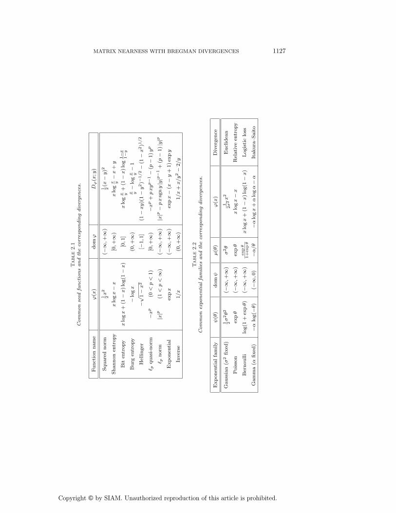
If each ϕn is Legendre, then the weighted sum is also Legendre. In the most commonsituation, the weights are constant and all the ϕn are identical. In Table 2.1 welist some important Legendre functions on R that may be used to build separabledivergences. These examples are adapted from [4] and [2]. Several of the divergencesin Table 2.1 have names. We have already discussed the Euclidean divergence andthe relative entropy. The bit entropy leads to a type of logistic loss, and the Burgentropy leads to the Itakura–Saito divergence.
Many of these univariate divergences are connected with well-known exponentialfamilies of probability distributions on R. See Table 2.2 for some key examples drawnfrom [2].
One fundamental divergence is genuinely multidimensional. Suppose that Q is apositive-definite operator that acts on X . We may construct a quadratic divergenceon X from the seed function ϕ(x) = 1
2 〈Qx,x〉, resulting in
Dϕ(x;y) = 12 〈Q (x− y),x− y〉 .
Copyright © by SIAM. Unauthorized reproduction of this article is prohibited.
MATRIX NEARNESS WITH BREGMAN DIVERGENCES 1127
Table
2.1
Com
mon
seed
funct
ions
and
the
corr
espo
ndin
gdiv
erge
nce
s.
Funct
ion
nam
eϕ(x
)dom
ϕD
ϕ(x
;y)
Square
dnorm
1 2x2
(−∞
,+∞
)1 2(x
−y)2
Shannon
entr
opy
xlo
gx−
x[0,+
∞)
xlo
gx y−
x+
y
Bit
entr
opy
xlo
gx
+(1
−x)lo
g(1
−x)
[0,1
]x
log
x y+
(1−
x)lo
g1−x
1−y
Burg
entr
opy
−lo
gx
(0,+
∞)
x y−
log
x y−
1
Hel
linger
−√
1−
x2
[−1,1
](1
−xy)(
1−
y2)−
1/2−
(1−
x2)1
/2
� pquasi
-norm
−xp
(0<
p<
1)
[0,+
∞)
−xp
+pxyp−
1−
(p−
1)yp
� pnorm
|x|p
(1<
p<
∞)
(−∞
,+∞
)|x|p
−px
sgny|y|p
−1
+(p
−1)|y|p
Exponen
tial
expx
(−∞
,+∞
)ex
px−
(x−
y+
1)ex
py
Inver
se1/x
(0,+
∞)
1/x
+x/y2−
2/y
Table
2.2
Com
mon
expo
nen
tialfa
milie
sand
the
corr
espo
ndin
gdiv
erge
nce
s.
Exponen
tialfa
mily
ψ(θ
)dom
ψμ(θ
)ϕ(x
)D
iver
gen
ce
Gauss
ian
(σ2
fixed
)1 2σ
2θ2
(−∞
,+∞
)σ
2θ
12σ2x2
Eucl
idea
n
Pois
son
expθ
(−∞
,+∞
)ex
pθ
xlo
gx−
xR
elative
entr
opy
Ber
noulli
log(1
+ex
pθ)
(−∞
,+∞
)expθ
1+
expθ
xlo
gx
+(1
−x)lo
g(1
−x)
Logis
tic
loss
Gam
ma
(αfixed
)−α
log(−
θ)
(−∞
,0)
−α/θ
−α
logx
+α
logα−
αIt
akura
–Saito
Copyright © by SIAM. Unauthorized reproduction of this article is prohibited.
1128 INDERJIT S. DHILLON AND JOEL A. TROPP
This divergence is connected to the exponential family of multivariate Gaussian dis-tributions with covariance matrix Q−1. In the latter context, the square root of thisdivergence is often referred to as the Mahalanobis distance in statistics [29]. Othermultidimensional examples arise when we compose the Euclidean norm with another
function. For instance, one might consider the convex function ϕ(x) = −√
1 − ‖x‖22
defined on the Euclidean unit ball. It yields the Hellinger-like divergence
Dϕ(x;y) =1 − 〈x,y〉√
1 − ‖y‖22
−√
1 − ‖x‖22.
2.6. Matrix divergences. Hermitian matrices admit a rich variety of diver-gences that were first studied in [4] using the methods of Lewis [27]. Let H bethe space of N × N Hermitian matrices equipped with the real-linear inner product〈X,Y 〉 = Re TrXY ∗. Define the function λ : H → R
N that maps a Hermitian ma-trix to the vector listing its eigenvalues in algebraically decreasing order. Let ϕ be aclosed, proper, convex function on R
N that is invariant under coordinate permutation.That is, ϕ(x) = ϕ(Px) for every permutation matrix P .
By composing ϕ with the eigenvalue map, we induce a real-valued function onHermitian matrices. As the following theorem elaborates, the induced map has thesame convexity properties as the function ϕ. Therefore, the induced map can beused as a seed function to define a Bregman divergence on the space of Hermitianmatrices.
Theorem 2 (Lewis [27, 26]). The induced map ϕ◦λ has the following properties:
1. If ϕ is closed and convex, then the induced map is closed and convex.2. The domain of ϕ ◦ λ is the inverse image under λ of domϕ.3. The conjugate of the induced map satisfies the relation (ϕ ◦ λ)∗ = ϕ∗ ◦ λ.4. The induced map is differentiable at X if and only if ϕ is differentiable at
λ(X). If X has eigenvalue decomposition U {diagλ(X)}U∗, then
∇(ϕ ◦ λ)(X) = U {diag∇ϕ(λ(X))}U∗.
In fact, this formula holds even if ϕ is not convex.5. The induced map is Legendre if and only if ϕ is Legendre.
Related results hold for the singular value map, provided that ϕ is also absolutelyinvariant. That is, ϕ(x) = ϕ(|x|) for all x in R
N , where |·| is the componentwiseabsolute value.
Unitarily invariant matrix norms provide the most basic examples of inducedmaps. Indeed, item 3 of the last theorem generalizes von Neumann’s famous resultabout dual norms of unitarily invariant prenorms [21, 438ff.].
An exquisite example of a matrix divergence arises from ϕ(x) = −∑
n log xn.The induced map is (ϕ ◦ λ)(X) = − log detX, whose domain is the positive-definitecone. Since ∇(ϕ ◦ λ)(X) = −X−1, the resulting divergence is
(2.7) D�d(X;Y ) =⟨X,Y −1
⟩− log detXY −1 −N.
Intriguingly, certain projections with respect to this divergence can be computedanalytically. See subsection 3.3 for details.
Copyright © by SIAM. Unauthorized reproduction of this article is prohibited.
MATRIX NEARNESS WITH BREGMAN DIVERGENCES 1129
Another important example arises from the negative Shannon entropy ϕ(x) =∑n xn log xn − xn. The induced map is (ϕ ◦ λ)(X) = Tr (X logX − X), whose
domain is the positive-semidefinite cone. This matrix function arises in quantummechanics, where it is referred to as the von Neumann entropy [31]. It yields thedivergence
(2.8) DvN(X;Y ) = Tr [X(logX − logY ) −X + Y ],
which we will call the von Neumann divergence. In the quantum mechanics literature,this divergence is referred to as the quantum relative entropy [31]. This formula doesnot literally hold if either matrix is singular, but a limit argument shows that thedivergence is finite precisely when the null space of X contains the null space of Y .
When the seed function ϕ is separable, matrix divergences can be expressed ina way that emphasizes the distinct roles of the eigenvalues and eigenvectors. Inparticular, take ϕ(x) =
∑n ϕ(xn) and assume that X has eigenpairs (um, μm) and
that Y has eigenpairs (vn, νn). Then
Dϕ◦λ(X;Y ) =∑
m,n|〈um,vn〉|2 [ϕ(μm) − ϕ(νn) − ϕ′(νn)(μm − νn)]
=∑
m,n|〈um,vn〉|2Dϕ(μm; νn).
In words, the matrix divergence adds up the scalar divergences between pairs ofeigenvalues, weighted by the squared cosine of the angle between the correspondingeigenvectors.
3. Computing Bregman projections. It is not straightforward to computethe Bregman projection onto a general convex set. Unless additional structure ispresent, the best approach may be to apply standard convex optimization techniques.In this section, we discuss how to develop numerical methods for the basic problemof projecting onto a hyperplane or a halfspace. As we will see in sections 4 and 6, theprojection onto an intersection of convex sets can be broken down into a sequence ofprojections onto the individual sets. Combining the two techniques, we can find theprojection onto any affine space or polyhedral convex set.
3.1. Projection onto a hyperplane. There is an efficient way to computethe Bregman projection onto a hyperplane. The key idea is to dualize the Bregmanprojection problem to obtain a nice one-dimensional problem. This approach can alsobe extended to produce the projection onto a halfspace because the convexity of thedivergence implies that the projection lies on the boundary whenever the initial pointis outside the halfspace.
We must solve the following convex program:
(3.1) minx
Dϕ(x;y) subject to 〈a,x〉 = α.
To ensure that this problem is well posed, we assume that ri(domϕ) contains a feasiblepoint. A necessary and sufficient condition on the solution x� of (3.1) is that theequation
∇xDϕ(x;y) = ξ∇x (〈a,x〉 − α)
hold for a (unique) Lagrange multiplier ξ ∈ R. The gradient of the divergence is∇ϕ(x) −∇ϕ(y), resulting in the equation
∇ϕ(x�) = ξa + ∇ϕ(y).
Copyright © by SIAM. Unauthorized reproduction of this article is prohibited.
1130 INDERJIT S. DHILLON AND JOEL A. TROPP
The gradient of a Legendre function ϕ is a bijection from domϕ to domϕ∗, and itsinverse is the gradient of the conjugate [35, Thm. 26.5]. Thus we obtain an explicitexpression for the Bregman projection as a function of the unknown multiplier:
(3.2) x� = ∇ϕ∗(ξa + ∇ϕ(y)).
Form the inner product with a and enforce the constraint to reach
(3.3) 〈∇ϕ∗(ξa + ∇ϕ(y)),a〉 − α = 0.
Now, the left-hand side of this equation is the derivative of the strictly convex, uni-variate function
(3.4) J(ξ) = ϕ∗(ξa + ∇ϕ(y)) − αξ.
There is an implicit constraint that the argument of ϕ∗ must lie within its domain. Inview of (3.3), it becomes clear that the Lagrange multiplier is the unique minimizerof J . That is,
ξ� = arg minξ J(ξ).
Once we have determined the Lagrange multiplier, we introduce it into (3.2) to obtainthe Bregman projection.
The best numerical method for minimizing J depends strongly on the choice ofthe seed function ϕ. In some cases, the derivative(s) of J may be difficult to evaluate.The second derivative may even fail to exist. To that end, we offer several observationsthat may be valuable.
1. The domain of J contains a neighborhood of zero since J(0) = 〈y,∇ϕ(y)〉 −ϕ(y).
2. Since ϕ∗ is a Legendre function, the first derivative of J always exists. Asshown in (3.3),
J ′(ξ) = 〈∇ϕ∗(ξa + ∇ϕ(y)),a〉 − α.
3. When the Hessian of ϕ∗ exists, we have
J ′′(ξ) = a∗ {∇2ϕ∗(ξa + ∇ϕ(y))}a.
4. When the seed function ϕ is separable, the Hessian ∇2ϕ∗ is diagonal.The next two subsections provide examples that illustrate some of the issues involvedin optimizing J .
3.2. Example: Relative entropy. Suppose that we wish to produce the Breg-man projection of a nonnegative vector y onto the hyperplane C = {x : 〈a,x〉 = α}with respect to the relative entropy. This divergence arises from the seed functionϕ(x) =
∑n xn log xn − xn, whose conjugate is ϕ∗(θ) =
∑n exp(θn). To identify the
Lagrange multiplier, we must minimize
J(ξ) =∑
nyn exp(ξan) − αξ,
whose derivatives are
J ′(ξ) =∑
nanyn exp(ξan) − α,
J ′′(ξ) =∑
na2nyn exp(ξan).
Copyright © by SIAM. Unauthorized reproduction of this article is prohibited.
MATRIX NEARNESS WITH BREGMAN DIVERGENCES 1131
These functions are all simple to evaluate, so it is best to use the Newton methodpreceded by a bracketing phase [32]. Once we have found the minimizer ξ�, theBregman projection is
PC(y) = y · exp(ξ�a),
where · represents the Hadamard product and the exponential is performed compo-nentwise.
3.3. Example: Log-determinant divergence. Here is a more sophisticatedexample that involves the log-determinant divergence. The divergence arises fromthe seed function ϕ(X) = − log det(X), whose domain is the positive-definite coneand whose gradient is ∇ϕ(X) = −X−1. The conjugate function ϕ∗(Θ) = N −log det(−Θ), whose domain is the negative-definite cone and whose gradient satisfies∇ϕ∗(Θ) = −Θ−1.
Suppose we need to project the positive-definite matrix Y onto the hyperplane
C = {X : 〈A,X〉 = α}, where A = A∗.
We must minimize
J(ξ) = N − log det(Y −1 − ξA) − αξ,
while ensuring that Y −1 − ξA is positive definite.Let Y = LL∗, and abbreviate W = L∗AL, which is singular whenever A is rank
deficient. Then the derivatives of J can be expressed as
J ′(ξ) = Tr (W (I − ξW )−1) − α,
J ′′(ξ) = Tr ((W (I − ξW )−1
)2).
In general, J and its derivatives are all costly. It appears that the most efficient wayto calculate them for multiple values of the scalar ξ is to preprocess W to extract itseigenvalues {λn}. It follows that
J ′(ξ) =
(∑n
λn
1 − λnξ
)− α,
J ′′(ξ) =∑
n
(λn
1 − λnξ
)2
.
It is worth cautioning that domJ = {ξ : ξ < 1/maxn λn} since the matrix I − ξWmust remain positive definite.
Once again, we see that a guarded or damped Newton method is the best way tooptimize J . Given the solution ξ�, the Bregman projection is
PC(Y ) = L(I − ξ�W )−1L∗.
We can reuse the eigenvalue decomposition to accelerate this final computation.As shown in [25], these calculations simplify massively when the constraint matrix
has rank one: A = aa∗. In this case, we can find the zero of J ′ analytically becausea∗Y a is the only nonzero eigenvalue of W . Then the Sherman–Morrison formuladelivers an explicit expression for the projection:
PC(Y ) = Y +a∗Y a− α
(a∗Y a)2(Y a)(Y a)∗.
The cost of performing the projection totals O(N2).
Copyright © by SIAM. Unauthorized reproduction of this article is prohibited.
1132 INDERJIT S. DHILLON AND JOEL A. TROPP
4. The successive projection algorithm for affine constraints. Now wedescribe an algorithm for solving (1.1) in the special case that the constraint sets areall affine spaces. In the next section, we will present some concrete problems to whichthis algorithm applies. The case of general convex constraint sets will be addressedafterward. We frame the following hypotheses.
Assumption A.1
The divergence: ϕ is a convex function of Legendre type
domϕ∗ is an open set
The constraints: C1, C2, . . . , CK are affine spaces with intersection C
Constraint qualification: C ∩ ri(domϕ) is nonempty
Note that, by the results of subsection 2.3, all Bregman divergences that arisefrom regular exponential families satisfy Assumption A.1.
Given an input y0 from ri(domϕ), we seek the Bregman projection of y0 ontothe intersection C of the affine constraints. In general, it may be difficult to producePC(y0). Nevertheless, if the basic sets C1, . . . , CK are chosen well, it may be relativelystraightforward to calculate the Bregman projection onto each basic set. This heuristicsuggests an algorithm: Project successively onto each basic set in the hope that thesequence of iterates will converge to the Bregman projection onto the intersection.To make this approach work in general, it is clear that we must choose every setan infinite number of times, so we add one more requirement to Assumption A.1 asfollows.
Assumption A.2
The control mapping: r : N → {1, . . . ,K} is a sequence that takes eachoutput value an infinite number of times
Together, Assumptions A.1 and A.2 will be referred to as Assumption A. Here is aformal statement of the algorithm.
Algorithm A (successive projection). Suppose that Assumption A is in force.Choose an input vector y0 from ri(domϕ), and form a sequence of iterates via suc-cessive Bregman projection:
yt = PCr(t)(yt−1).
Then the sequence of iterates {yt} converges in norm to PC(y0).We present a short proof that this algorithm is correct. We refer to the article [4]
for the argument that the sequence converges, and we extend the elegant proof from[12] to show that the limit of the sequence yields the Bregman projection.
Proof. Suppose that a is an arbitrary point in C ∩domϕ. Since the seed functionϕ is Legendre, Bregman projections with respect to the divergence fall in the relativeinterior of domϕ. In particular, each iterate yt belongs to ri(domϕ). Therefore, wemay apply the Pythagorean theorem (2.4) to see that
Dϕ(a;yt−1) = Dϕ(a;yt) + Dϕ(yt;yt−1).
Observe that this equation defines a recurrence, which we may solve to obtain
Dϕ(a;y0) = Dϕ(a;yt) +∑t
i=1D(yi;yi−1).
Copyright © by SIAM. Unauthorized reproduction of this article is prohibited.
MATRIX NEARNESS WITH BREGMAN DIVERGENCES 1133
Under Assumption A, Theorem 8.1 of [4] shows that the sequence of iterates generatedby Algorithm A converges to a point y in C ∩ ri(domϕ). Since the divergence iscontinuous in its second argument, we may take limits to reach
Dϕ(a;y0) = Dϕ(a;y) +∑∞
i=1Dϕ(yi;yi−1).
We chose a arbitrarily from C ∩ domϕ, so we may replace a by y to see that theinfinite sum equals Dϕ(y;y0). It follows that
Dϕ(a;y0) = Dϕ(a;y) + Dϕ(y;y0).
This equation holds for each point a in C ∩ domϕ, so we see that y meets thevariational characterization (2.4) of PC(y0). Therefore, y is the Bregman projectionof y0 onto C.
If the sets {Ck} are not affine, then Algorithm A will generally fail to produce theBregman projection of y0 onto the intersection C. In section 6, we will discuss a moresophisticated iterative algorithm for solving this problem. Nevertheless, for generalclosed, convex constraint sets, the sequence of iterates generated by the successiveprojection algorithm still converges to a point in C ∩ ri(domϕ) [4, Theorem 8.1].
To obtain the convergence guarantee for Algorithm A, it may be necessary towork in an affine subspace of the ambient inner-product space. This point becomesimportant when computing the projections of nonnegative (as opposed to positive)vectors with respect to the relative entropy. It arises again when studying projectionsof rank-deficient matrices with respect to the von Neumann divergence. We will touchon this issue in subsections 5.1 and 5.3.
5. Examples with affine constraints. This section presents three matrixnearness problems with affine constraints. The first requests the nearest contingencytable with fixed marginals. A special case is to produce the nearest doubly stochasticmatrix with respect to relative entropy. For this problem, the successive projectionalgorithm is identical to Kruithof’s famous diagonal scaling algorithm [24, 13].
The second problem centers on a matrix nearness problem from data analysis,namely, that of finding matrix approximations based on the MBI principle, which isa generalization of Jaynes’ maximum entropy principle [23].
The third problem shows how to construct the correlation matrix closest to a givenpositive-semidefinite matrix with respect to some matrix divergences. For reference,a correlation matrix is a positive-semidefinite matrix with a unit diagonal.
5.1. Contingency tables with fixed marginals. A contingency table is an ar-ray that exhibits the joint probability mass function of a collection of discrete randomvariables. A nonnegative rectangular matrix may be viewed as the contingency tablefor two discrete random variables. We will focus on this case since higher-dimensionalcontingency tables essentially are no more complicated.
Suppose that pAB is the joint probability mass function of two random variablesA and B with sample spaces {1, 2, . . . ,M} and {1, 2, . . . , N}. We use X to denotethe M ×N contingency table whose entries are
xmn = pAB(A = m and B = n).
A marginal of pAB is a linear function of X. The most important marginals ofpAB are the vector of row sums X e, which gives the distribution of A, and the vectorof column sums eT X, which gives the distribution of B. Here, e is a conformal vector
Copyright © by SIAM. Unauthorized reproduction of this article is prohibited.
1134 INDERJIT S. DHILLON AND JOEL A. TROPP
of ones. The distribution of A conditioned on B = n is given by the nth column ofX, and the distribution of B conditioned on A = m is given by the mth row of X.
However, we consider the more general case of arbitrary nonnegative matrices—wetreat X as a member of the collection of M×N real matrices equipped with the innerproduct 〈X,Y 〉 = TrXY T . Note that, for the above probabilistic interpretation, Xmust be scaled so that its entries sum to 1.
A common problem is to use an initial estimate to produce a contingency tablethat has fixed marginals. In this setting, nearness is typically measured with relativeentropy
D(X;Y ) =∑
m,n
[xmn log
xmn
ymn− xmn + ymn
].
An important special case is to find the doubly stochastic matrix nearest to a non-negative square matrix Y0. In this case, we have two constraint sets
C1 = {X : X e = e} and C2 = {X : eT X = eT }.
It is clear that the intersection C = C1 ∩ C2 contains the set of doubly stochasticmatrices. In fact, every nonnegative matrix in C is doubly stochastic. Using (2.6),it is easy to see that Bregman projection of a matrix onto C1 with respect to therelative entropy is accomplished by rescaling the rows so that each row sums to one.Likewise, Bregman projection of a matrix onto C2 is accomplished by rescaling thecolumns. Beginning with Y0, the successive projection algorithm alternately rescalesthe rows and columns. This procedure, of course, is the diagonal scaling algorithm ofKruithof [24, 13], sometimes called Sinkhorn’s algorithm [36]. Our approach yields ageometric interpretation of the algorithm as a method for solving a matrix nearnessproblem by alternating Bregman projections. It is interesting that the nonnegativityconstraint is implicitly enforced by the domain of the relative entropy. This viewpointcan be traced to the work of Ireland and Kullback [22].
There is still a subtlety that requires attention. Assumption A apparently requiresthat C contain a matrix with strictly positive entries and that the input matrix Y0 bestrictly positive. In fact, we may relax these premises. A nonnegative matrix whosezero pattern does not cover the zero pattern of Y0 has an infinite divergence fromY0. Therefore, we may as well restrict our attention to the linear space of matriceswhose zero pattern covers that of Y0. Now we see that the constraint qualification inAssumption A requires that C contain a matrix with exactly the same zero patternas Y0. If it does, the algorithm will still converge to the Bregman projection of Y0
onto the doubly stochastic matrices. Determining whether the constraint qualificationholds will generally involve a separate investigation [30].
It is also worth noting that Algorithm A encompasses other iterative methods forscaling to doubly stochastic form. At each step, for example, one might rescale onlythe row or column whose sum is most inaccurate. Parlett and Landis have consideredalgorithms of this sort [33]. The problem of scaling to have other row and columnsums also fits neatly into our framework, and it has the same geometric interpretation.
5.2. MBI and matrix approximation. This section discusses a novel matrixnearness problem that arises in data analysis. Given a collection of vectors X ={x1,x2, . . . ,xN} ⊂ domϕ, the Bregman information [2] of the collection is defined tobe
(5.1) Iϕ(X) =∑N
j=1wj Dϕ(xj ;μ),
Copyright © by SIAM. Unauthorized reproduction of this article is prohibited.
MATRIX NEARNESS WITH BREGMAN DIVERGENCES 1135
where w1, w2, . . . , wN are nonnegative weights that sum to one, and μ is the (weighted)arithmetic mean of the collection, i.e., μ =
∑j wj xj . Bregman information gener-
alizes the notion of the variance, σ2 = N−1∑
j ‖xj − μ‖22, of a Gaussian random
variable (where each wj = N−1). When Dϕ is the relative entropy, the Bregmaninformation that arises with an appropriate choice of weights is called mutual infor-mation, a fundamental quantity in information theory [11].
Bregman information exhibits an interesting connection with Jensen’s inequalityfor a convex function ϕ: ∑
jwj ϕ(xj) ≥ ϕ
(∑jwj xj
).
Substituting μ =∑
j wj xj , we see that the difference between the two sides of theforegoing relation satisfies∑
jwj ϕ(xj) − ϕ(μ) =
∑jwj ϕ(xj) − ϕ(μ) −
⟨∇ϕ(μ),
∑jwjxj − μ
⟩=∑
jwj
[ϕ(xj) − ϕ(μ) − 〈∇ϕ(μ),xj − μ〉
]= Iϕ(X).(5.2)
In words, the Bregman information is the disparity between the two sides of Jensen’sinequality. Equation (5.2) can also be viewed as a generalization of the relationshipbetween the variance and the arithmetic mean,
σ2 = N−1∑
j‖xj‖2
2 − ‖μ‖22 .
Let us describe an application of Bregman information in data analysis. In thisfield, matrix approximations play a central role. Unfortunately, many common ap-proximations destroy essential structure in the data matrix. For example, considerthe k-truncated singular value decomposition (TSVD), which provides the best rank-k Frobenius-norm approximation of a matrix. In information retrieval applications,however, the matrix that describes the co-occurrence of words and documents is bothsparse and nonnegative. The TSVD ruins both of these properties. In this setting,the Frobenius norm is meaningless; relative entropy is the correct divergence measureaccording to the unigram or multinomial language model.
We may also desire that the matrix approximation satisfy some additional con-straints. For instance, it may be valuable for the approximation to preserve marginals(i.e., linear functions) of the matrix entries. Let us formalize this idea. Suppose that
Y is an M×N data matrix. We seek an approximation X that satisfies the constraints
Ck = {X : 〈X,Ak〉 = 〈Y ,Ak〉} k = 1, . . . ,K,
where each Ak is a fixed constraint matrix. We will write C =⋂
k Ck. As an example,X can be required to preserve the row and/or column sums of Y .
Many different matrices, including the original matrix Y , may satisfy these con-straints. Clearly, a good matrix approximation should involve some reduction in thenumber of parameters used to represent the matrix. The key question is to decide howto produce the right approximation from C. One rational approach invokes the princi-ple of minimum Bregman information (MBI) [1], which states that the approximationshould be the (unique) solution of the problem
(5.3) minX∈C
Iϕ(X) = minX∈C
∑m,n
wmn Dϕ(xmn, μ),
Copyright © by SIAM. Unauthorized reproduction of this article is prohibited.
1136 INDERJIT S. DHILLON AND JOEL A. TROPP
where wmn are prespecified weights and μ =∑
m,n wmnxmn. If the weights wmn andthe matrix entries xmn are both sets of nonnegative numbers that sum to one, andif the Bregman divergence is the relative entropy, then the MBI principle reduces toJaynes’ maximum entropy principle [23]. Thus, the MBI principle tries to obtain asuniform an approximation as possible subject to the specified constraints. Note thatproblem (5.3) can be readily solved by the successive projection algorithm.
Next, we consider an important and natural source of constraints. Clustering isthe problem of partitioning a set of objects into clusters, where each cluster contains“similar” objects. Data matrices often capture the relationships between two sets ofobjects, such as word–document matrices in information retrieval and gene-expressionmatrices in bioinformatics. In such applications, it is often desirable to solve the co-clustering problem, i.e., to simultaneously cluster the rows and columns of a datamatrix. Formally, a co-clustering (ρ, γ) is a partition of the rows into I row clustersρ1, . . . , ρI and the columns into J column clusters γ1, . . . , γJ , i.e.,⋃I
i=1ρi = {1, 2, . . . ,M}, where ρi ∩ ρ� = ∅ for i �= �,
⋃J
j=1γj = {1, 2, . . . , N}, where γj ∩ γ� = ∅ for j �= �.
Given a coclustering, the rows belonging to row cluster ρ1 can be arranged first,followed by rows belonging to row cluster ρ2, etc. Similarly the columns can be re-ordered. This re-ordering has the effect of dividing the matrix into I · J subblocks,each of which is called a cocluster.
The coclustering problem is to search for the “best” possible row and columnclusters. One way to measure the quality of a coclustering is to associate it withits MBI matrix approximation. A natural constraint set C(ρ,γ) for the coclusteringproblem contains matrices that preserve marginals of all the I · J coclusters (localinformation) in addition to row and column marginals (global information). Withthis constraint set, a formal objective for the coclustering problem is to find (ρ, γ),which corresponds to the best possible MBI approximation:
(5.4) minρ,γ
Dϕ(Y ;X(ρ,γ)), where X(ρ,γ) = arg minX∈C(ρ,γ)
Iϕ(X).
This formulation yields an optimal coclustering as well as its associated MBI matrixapproximation. The quality of such matrix approximations is a topic for further study.Note that problem (5.4) requires a combinatorial search, and it is known to be NP-complete. The most familiar clustering formulation, namely, the k-means problem, isthe special case of (5.4) obtained from the Euclidean divergence, the choice J = N ,and the condition of preserving cocluster sums.
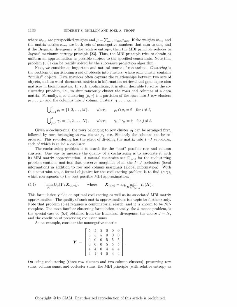
As an example, consider the nonnegative matrix
Y =
⎡⎢⎢⎢⎢⎢⎢⎣
5 5 5 0 0 05 5 5 0 0 00 0 0 5 5 50 0 0 5 5 54 4 0 4 4 44 4 4 0 4 4
⎤⎥⎥⎥⎥⎥⎥⎦.
On using coclustering (three row clusters and two column clusters), preserving rowsums, column sums, and cocluster sums, the MBI principle (with relative entropy as
Copyright © by SIAM. Unauthorized reproduction of this article is prohibited.
MATRIX NEARNESS WITH BREGMAN DIVERGENCES 1137
the Bregman divergence) yields the matrix approximation
X1 =
⎡⎢⎢⎢⎢⎢⎢⎣
5.4 5.4 4.2 0 0 05.4 5.4 4.2 0 0 0
0 0 0 4.2 5.4 5.40 0 0 4.2 5.4 5.4
3.6 3.6 2.8 2.8 3.6 3.63.6 3.6 2.8 2.8 3.6 3.6
⎤⎥⎥⎥⎥⎥⎥⎦.
Note that this approximation has rank two and preserves nonnegativity as well asmost of the nonzero structure of Y . It can be verified that all the cocluster sums,row sums, and column sums of X1 match those of Y . In contrast, the rank-two SVDapproximation
X2 =
⎡⎢⎢⎢⎢⎢⎢⎣
5.09 5.09 4.66 −0.69 0.29 0.295.09 5.09 4.66 −0.69 0.29 0.290.29 0.29 −0.69 4.66 5.09 5.090.29 0.29 −0.69 4.66 5.09 5.093.04 3.04 1.98 3.51 4.41 4.414.41 4.41 3.51 1.98 3.04 3.04
⎤⎥⎥⎥⎥⎥⎥⎦
preserves neither the nonnegativity, the nonzero structure, nor the marginals of Y .
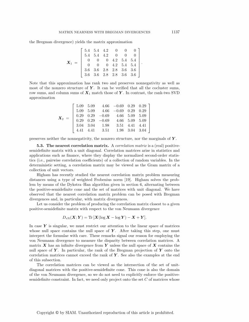
5.3. The nearest correlation matrix. A correlation matrix is a (real) positive-semidefinite matrix with a unit diagonal. Correlation matrices arise in statistics andapplications such as finance, where they display the normalized second-order statis-tics (i.e., pairwise correlation coefficients) of a collection of random variables. In thedeterministic setting, a correlation matrix may be viewed as the Gram matrix of acollection of unit vectors.
Higham has recently studied the nearest correlation matrix problem measuringdistances using a type of weighted Frobenius norm [19]. Higham solves the prob-lem by means of the Dykstra–Han algorithm given in section 6, alternating betweenthe positive-semidefinite cone and the set of matrices with unit diagonal. We haveobserved that the nearest correlation matrix problem can be posed with Bregmandivergences and, in particular, with matrix divergences.
Let us consider the problem of producing the correlation matrix closest to a givenpositive-semidefinite matrix with respect to the von Neumann divergence
DvN(X;Y ) = Tr [X(logX − logY ) −X + Y ].
In case Y is singular, we must restrict our attention to the linear space of matriceswhose null space contains the null space of Y . After taking this step, one mustinterpret the formulae with care. These remarks signal our reason for employing thevon Neumann divergence to measure the disparity between correlation matrices. Amatrix X has an infinite divergence from Y unless the null space of X contains thenull space of Y . In particular, the rank of the Bregman projection of Y onto thecorrelation matrices cannot exceed the rank of Y . See also the examples at the endof this subsection.
The correlation matrices can be viewed as the intersection of the set of unit-diagonal matrices with the positive-semidefinite cone. This cone is also the domainof the von Neumann divergence, so we do not need to explicitly enforce the positive-semidefinite constraint. In fact, we need only project onto the set C of matrices whose
Copyright © by SIAM. Unauthorized reproduction of this article is prohibited.
1138 INDERJIT S. DHILLON AND JOEL A. TROPP
diagonal entries all equal one. It is natural to view C as the intersection of the affineconstraint sets
Ck = {X : xkk = 1}.
There is no explicit formula for the projection of a matrix Y onto the set Ck, butthe discussion in section 3 shows that we can solve the problem by minimizing thefunction (3.4), which, in this example, reads
(5.5) J(ξ) = Tr exp{logY + ξ ekeTk } − ξ,
where ek is the kth canonical basis vector. Given the minimizer ξ�, the projection ofY onto Ck is
(5.6) PCk(Y ) = exp{logY + ξ� eke
Tk }.
Beware that one cannot read these formulae literally when Y is rank deficient! Inany case, the numerical calculations are not trivial to perform. In order to apply theNewton method, the second derivative of J is needed, which is more involved due tothe noncommutativity of matrix multiplication.
Unfortunately, treating these issues in detail is beyond the scope of this paper.
There is an interesting special case that can be treated without optimization:the von Neumann projection of a matrix with constant diagonal onto the correlationmatrices can always be obtained by rescaling. In particular, the projection preservesthe zero pattern of the matrix and the eigenvalue distribution. To verify this point,suppose the diagonal entries of Y equal α, and set X = α−1Y . According to theKarush–Kuhn–Tucker conditions, X is the Bregman projection of Y onto the set Cprovided that ∇XDvN(X;Y ) is diagonal. The latter gradient equals logX−logY +I,and a short calculation completes the argument. In contrast, the Frobenius normprojection of a matrix with constant diagonal does not preserve its nonzero structureor eigenvalue distribution. As an example, let Y be the 4 × 4 symmetric tridiagonalToeplitz matrix with 2’s on the diagonal and −1’s on the off-diagonal. The nearestcorrelation matrix to it, in the Frobenius norm, equals (to the figures shown)
⎡⎢⎢⎣
1.0000 −0.8084 0.1916 0.1068−0.8084 1.0000 −0.6562 0.1916
0.1916 −0.6562 1.0000 −0.80840.1068 0.1916 −0.8084 1.0000
⎤⎥⎥⎦ .
As a second example, draw a random orthogonal matrix Q and form the rank-deficient matrix Y = Q diag (1, 10−3, 10−6, 0)QT . For instance,
Y =
⎡⎢⎢⎣
.18335 −.15180 .08258 −.34620−.15180 .12606 −.06887 .28655.08258 −.06887 .03786 −.15582
−.34620 .28655 −.15582 .65373
⎤⎥⎥⎦ .
Copyright © by SIAM. Unauthorized reproduction of this article is prohibited.
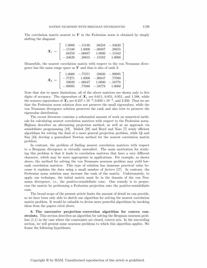
MATRIX NEARNESS WITH BREGMAN DIVERGENCES 1139
The correlation matrix nearest to Y in the Frobenius norm is obtained by simplyshifting the diagonal:
X1 =
⎡⎢⎢⎣
1.0000 −.15180 .08258 −.34620−.15180 1.0000 −.06887 .28655.08258 −.06887 1.0000 −.15582
−.34620 .28655 −.15582 1.0000
⎤⎥⎥⎦ .
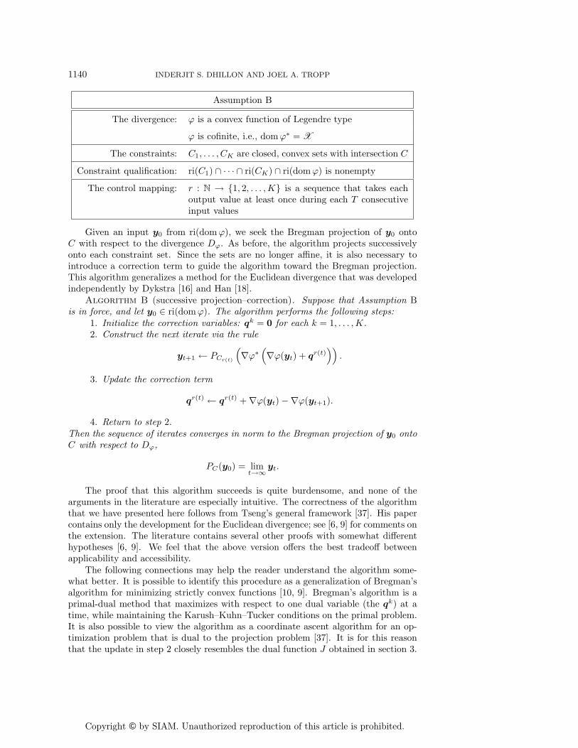
Meanwhile, the nearest correlation matrix with respect to the von Neumann diver-gence has the same range space as Y and thus is also of rank 3:
X2 =
⎡⎢⎢⎣
1.0000 −.77271 .59020 −.99995−.77271 1.0000 −.96847 .77080.59020 −.96847 1.0000 −.58778
−.99995 .77080 −.58778 1.0000
⎤⎥⎥⎦ .
Note that due to space limitations, all of the above matrices are shown only to fivedigits of accuracy. The eigenvalues of X1 are 0.611, 0.851, 0.951, and 1.588, whilethe nonzero eigenvalues of X2 are 0.457× 10⁻⁶, 0.650× 10⁻², and 3.350. Thus we seethat the Frobenius norm solution does not preserve the small eigenvalues, while thevon Neumann divergence solution preserves the rank and also tries to preserve theeigenvalue distribution.
The recent literature contains a substantial amount of work on numerical meth-ods for calculating nearest correlation matrices with respect to the Frobenius norm.Higham describes an alternating projection method, as well as an approach viasemidefinite programming [19]. Malick [28] and Boyd and Xiao [7] study efficientalgorithms for solving the dual of a more general projection problem, while Qi andSun [34] develop a generalized Newton method for the nearest correlation matrixproblem.
In contrast, the problem of finding nearest correlation matrices with respectto a Bregman divergence is virtually unstudied. The main motivation for study-ing this problem is that it leads to correlation matrices that have a very differentcharacter, which may be more appropriate in applications. For example, as shownabove, the method for solving the von Neumann nearness problem may yield low-rank correlation matrices. This type of solution has immense practical value be-cause it explains the data using a small number of factors [17]. In contrast, theFrobenius norm solution may increase the rank of the matrix. Unfortunately, toapply our technique, the initial matrix must lie in the domain of the von Neu-mann divergence, i.e., the positive-semidefinite cone. One remedy is to prepro-cess the matrix by performing a Frobenius projection onto the positive-semidefinitecone.
The broad scope of the present article limits the amount of detail we can provide,so we have been only able to sketch one algorithm for solving the nearest correlationmatrix problem. It would be valuable to devise more powerful algorithms by invokingideas from the papers cited above.
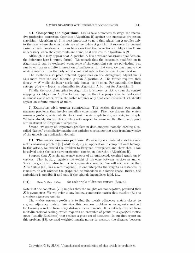
6. The successive projection–correction algorithm for convex con-straints. This section describes an algorithm for solving the Bregman nearness prob-lem (1.1) in the case where the constraints are closed, convex sets. In the succeedingsection, we will present some nearness problems to which this algorithm applies. Weframe the following hypotheses:
Copyright © by SIAM. Unauthorized reproduction of this article is prohibited.
1140 INDERJIT S. DHILLON AND JOEL A. TROPP
Assumption B
The divergence: ϕ is a convex function of Legendre type
ϕ is cofinite, i.e., domϕ∗ = X
The constraints: C1, . . . , CK are closed, convex sets with intersection C
Constraint qualification: ri(C1) ∩ · · · ∩ ri(CK) ∩ ri(domϕ) is nonempty
The control mapping: r : N → {1, 2, . . . ,K} is a sequence that takes eachoutput value at least once during each T consecutiveinput values
Given an input y0 from ri(domϕ), we seek the Bregman projection of y0 ontoC with respect to the divergence Dϕ. As before, the algorithm projects successivelyonto each constraint set. Since the sets are no longer affine, it is also necessary tointroduce a correction term to guide the algorithm toward the Bregman projection.This algorithm generalizes a method for the Euclidean divergence that was developedindependently by Dykstra [16] and Han [18].
Algorithm B (successive projection–correction). Suppose that Assumption Bis in force, and let y0 ∈ ri(domϕ). The algorithm performs the following steps:
1. Initialize the correction variables: qk = 0 for each k = 1, . . . ,K.2. Construct the next iterate via the rule
yt+1 ← PCr(t)
(∇ϕ∗
(∇ϕ(yt) + qr(t)
)).
3. Update the correction term
qr(t) ← qr(t) + ∇ϕ(yt) −∇ϕ(yt+1).
4. Return to step 2.Then the sequence of iterates converges in norm to the Bregman projection of y0 ontoC with respect to Dϕ,
PC(y0) = limt→∞
yt.
The proof that this algorithm succeeds is quite burdensome, and none of thearguments in the literature are especially intuitive. The correctness of the algorithmthat we have presented here follows from Tseng’s general framework [37]. His papercontains only the development for the Euclidean divergence; see [6, 9] for comments onthe extension. The literature contains several other proofs with somewhat differenthypotheses [6, 9]. We feel that the above version offers the best tradeoff betweenapplicability and accessibility.
The following connections may help the reader understand the algorithm some-what better. It is possible to identify this procedure as a generalization of Bregman’salgorithm for minimizing strictly convex functions [10, 9]. Bregman’s algorithm is aprimal-dual method that maximizes with respect to one dual variable (the qk) at atime, while maintaining the Karush–Kuhn–Tucker conditions on the primal problem.It is also possible to view the algorithm as a coordinate ascent algorithm for an op-timization problem that is dual to the projection problem [37]. It is for this reasonthat the update in step 2 closely resembles the dual function J obtained in section 3.
Copyright © by SIAM. Unauthorized reproduction of this article is prohibited.
MATRIX NEARNESS WITH BREGMAN DIVERGENCES 1141
6.1. Comparing the algorithms. Let us take a moment to weigh the succes-sive projection–correction algorithm (Algorithm B) against the successive projectionalgorithm (Algorithm A). It is most important to note that Algorithm A applies onlyto the case where the constraints are affine, while Algorithm B succeeds for generalclosed, convex constraints. It can be shown that the corrections in Algorithm B areunnecessary when the constraints are affine, so it reduces to Algorithm A [9].
Although it may appear that Algorithm A has a weaker constraint qualification,the difference here is purely formal. We remark that the constraint qualification inAlgorithm B can be weakened when some of the constraint sets are polyhedral, i.e.,can be written as a finite intersection of halfspaces. In that case, we may remove therelative interior from the polyhedral constraint sets in the constraint qualification.
The methods also place different hypotheses on the divergence; Algorithm Basks more from the seed function ϕ than Algorithm A. The former requires thatdomϕ∗ = X while the latter needs only domϕ∗ to be open. For example, the Burgentropy ϕ(x) = − log(x) is admissible for Algorithm A but not for Algorithm B.
Finally, the control mapping for Algorithm B is more restrictive than the controlmapping for Algorithm A. The former requires that the projections be performedin almost cyclic order, while the latter requires only that each constraint set shouldappear an infinite number of times.
7. Examples with convex constraints. This section discusses two matrixnearness problems that involve nonaffine constraints. First, we discuss the metricnearness problem, which elicits the closest metric graph to a given weighted graph.We have already studied this problem with respect to norms in [15]. Here, we expandour treatment to Bregman divergences.
Second, we study an important problem in data analysis, namely learning a so-called “kernel” or similarity matrix that satisfies constraints that arise from knowledgeof the underlying application domain.
7.1. The metric nearness problem. We recently encountered a striking newmatrix nearness problem [15] while studying an application in computational biology.In this article, we extend the problem to Bregman divergences and show that it canbe solved using the successive projection–correction algorithm (Algorithm B).
Suppose that X is the adjacency matrix of an undirected, weighted graph on Nvertices. That is, xmn registers the weight of the edge between vertices m and n.Since the graph is undirected, X is a symmetric matrix. We will also assume thatX is hollow (i.e., has a zero diagonal). If one interprets the weights as distances, itis natural to ask whether the graph can be embedded in a metric space. Indeed, theembedding is possible if and only if the triangle inequalities hold, i.e.,
(7.1) xmn ≤ xm� + x�n for each triple of distinct vertices (�,m, n).
Note that the condition (7.1) implies that the weights are nonnegative, provided thatX is symmetric. We will refer to any hollow, symmetric matrix that satisfies (7.1) asa metric adjacency matrix.
The metric nearness problem is to find the metric adjacency matrix closest toa given adjacency matrix. We view this nearness problem as an agnostic methodfor learning a metric from noisy distance measurements. It is entirely distinct frommultidimensional scaling, which requests an ensemble of points in a specified metricspace (usually Euclidean) that realizes a given set of distances. In our first report onthis problem [15], we used weighted matrix norms to measure the distance between
Copyright © by SIAM. Unauthorized reproduction of this article is prohibited.
1142 INDERJIT S. DHILLON AND JOEL A. TROPP
adjacency matrices. In this article, we will use Bregman divergences. Note that thedivergence is unrelated to the metric encoded in the entries of the adjacency matrix;the divergence is used to determine how much one adjacency matrix (i.e., graph)differs from another.
By this point, it should be clear how we propose to solve the metric nearnessproblem. We will work in the space of hollow, symmetric matrices. It is evidentthat the metric adjacency matrices from a closed, convex cone C. Clearly, C is theintersection of
(N3
)halfspaces:
C�mn = {X : xmn − xm� − x�n ≤ 0},
where �, m, and n index distinct vertices. Therefore, we may apply Algorithm B.To be concrete, we will consider Bregman projections with respect to the relative
entropy. For reference, the seed function is
ϕ(X) =∑
mn[xmn log xmn − xmn] ,
which has Fenchel conjugate
ϕ∗(Y ) =∑
mnexp ymn.
The divergence is
Dϕ(X;Y ) =∑
mn
[xmn log
xmn
ymn− xmn + ymn
].
This divergence has an interesting advantage over the Frobenius norm. If the originaladjacency matrix does not contain zero distances, then the projection on the metricadjacency matrices will not contain any zero distances. This fact ensures that thefinal matrix defines a genuine metric, rather than a pseudometric.
Algorithm B requires that we compute the Bregman projection of a matrix thathas the form X = ∇ϕ∗(∇ϕ(Yt) + Q�mn), where Q�mn is a dual variable. It is easyto check that this expression reduces to
X = Yt · exp ·(Q�mn),
where · is the Hadamard (i.e., componentwise) product and exp · is the Hadamardexponential. We will see that the dual variable Q�mn has at most six nonzero entries.Therefore, the matrix X differs from Yt in at most six places.
It is straightforward to calculate the Bregman projection Yt+1 of the matrix Xonto the constraint C�mn. If X already falls in the constraint set, then the projectionYt+1 = X. Otherwise, set δ =
√(xm� + x�n)/xmn. The entries of the projection
Yt+1 are identical to those of X except for the following six:
ymn = δ xmn ynm = ymn
ym� = xm�/δ y�m = ym�
y�n = x�n/δ yn� = y�n.
In words, the projection determines how much the triangle inequality is violated, andit distributes the deficit multiplicatively among the three edges.
Copyright © by SIAM. Unauthorized reproduction of this article is prohibited.
MATRIX NEARNESS WITH BREGMAN DIVERGENCES 1143
Finally, the algorithm updates the dual variable Q�mn associated with the con-straint using the formula
Q�mn ← Q�mn + log ·(Yt) − log ·(Yt+1)
where log · is the Hadamard logarithm. This update affects only six entries of Q�mn.In practice, we would store only the upper triangle of the adjacency matrices, so theupdate touches only three entries.
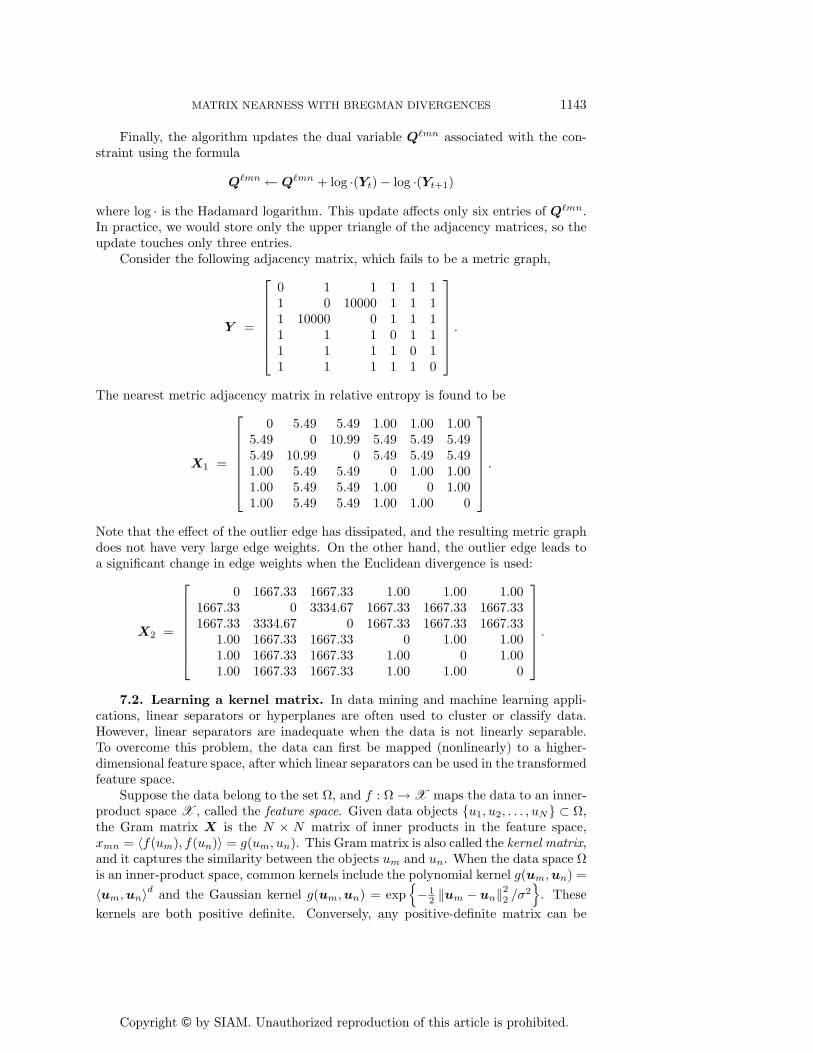
Consider the following adjacency matrix, which fails to be a metric graph,
Y =
⎡⎢⎢⎢⎢⎢⎢⎣
0 1 1 1 1 11 0 10000 1 1 11 10000 0 1 1 11 1 1 0 1 11 1 1 1 0 11 1 1 1 1 0
⎤⎥⎥⎥⎥⎥⎥⎦.
The nearest metric adjacency matrix in relative entropy is found to be
X1 =
⎡⎢⎢⎢⎢⎢⎢⎣
0 5.49 5.49 1.00 1.00 1.005.49 0 10.99 5.49 5.49 5.495.49 10.99 0 5.49 5.49 5.491.00 5.49 5.49 0 1.00 1.001.00 5.49 5.49 1.00 0 1.001.00 5.49 5.49 1.00 1.00 0
⎤⎥⎥⎥⎥⎥⎥⎦.
Note that the effect of the outlier edge has dissipated, and the resulting metric graphdoes not have very large edge weights. On the other hand, the outlier edge leads toa significant change in edge weights when the Euclidean divergence is used:
X2 =
⎡⎢⎢⎢⎢⎢⎢⎣
0 1667.33 1667.33 1.00 1.00 1.001667.33 0 3334.67 1667.33 1667.33 1667.331667.33 3334.67 0 1667.33 1667.33 1667.33
1.00 1667.33 1667.33 0 1.00 1.001.00 1667.33 1667.33 1.00 0 1.001.00 1667.33 1667.33 1.00 1.00 0
⎤⎥⎥⎥⎥⎥⎥⎦.
7.2. Learning a kernel matrix. In data mining and machine learning appli-cations, linear separators or hyperplanes are often used to cluster or classify data.However, linear separators are inadequate when the data is not linearly separable.To overcome this problem, the data can first be mapped (nonlinearly) to a higher-dimensional feature space, after which linear separators can be used in the transformedfeature space.
Suppose the data belong to the set Ω, and f : Ω → X maps the data to an inner-product space X , called the feature space. Given data objects {u1, u2, . . . , uN} ⊂ Ω,the Gram matrix X is the N × N matrix of inner products in the feature space,xmn = 〈f(um), f(un)〉 = g(um, un). This Gram matrix is also called the kernel matrix,and it captures the similarity between the objects um and un. When the data space Ωis an inner-product space, common kernels include the polynomial kernel g(um,un) =
〈um,un〉d and the Gaussian kernel g(um,un) = exp{− 1
2 ‖um − un‖22 /σ
2}
. These
kernels are both positive definite. Conversely, any positive-definite matrix can be
Copyright © by SIAM. Unauthorized reproduction of this article is prohibited.
1144 INDERJIT S. DHILLON AND JOEL A. TROPP
thought of as a kernel matrix [38]. In general, the set Ω can be arbitrary. Forexample, Ω might contain nucleotide sequences of varying lengths or phylogenetictrees or arbitrary graphs.
In many such situations, the choice of the kernel matrix is unclear. There is oftenan approximate kernel matrix Y0 that we wish to modify based on our informationabout the underlying data objects. This information may take various forms:
• known values for kernel entries (xmn = α),• known distances between objects in the feature space (xmm+xnn−2xmn = β),
or• known bounds on kernel entries (xmn ≤ xrs) or distances (xmm + xnn −
2xmn ≤ γ).Such constraints are typically obtained from the application domain, such as infor-mation about whether a pair of genes or proteins is functionally more similar thananother pair.
Suppose that we are given an approximate kernel matrix Y0. Our problem isto find the nearest positive-definite matrix to Y0 that satisfies linear equality andinequality constraints. The von Neumann divergence can be used as the nearnessmeasure:
DvN(X;Y ) = Tr [X(logX − logY ) −X + Y ].
Using the von Neumann divergence appears to be advantageous when the initial kernelmatrix Y0 is of low rank and it is desired that its null space be preserved [25]. Recallthat, in the low-rank case, the von Neumann divergence DvN(X;Y0) is finite onlywhen the null space of X contains the null space of Y0. Hence, both the null spaceconstraint and positive semidefiniteness are automatically enforced by the successiveprojection–correction algorithm.
8. Open problems and conclusions. The Bregman nearness problem is rel-atively unstudied, so it opens a rich vein of new questions. Here are some specificchallenges that deserve attention.
1. The matrix divergences described in subsection 2.6 offer an intriguing wayto compute distances between Hermitian matrices. It would be valuable tocharacterize different types of projections onto important sets of matrices,such as the positive-semidefinite cone, the nonnegative cone, or the set ofdiagonal matrices. This could lead to more efficient numerical methods forkey problems.
2. The algorithms described in this paper apply only to projections onto poly-hedral convex sets. Some important constraint sets—such as the positive-semidefinite cone—are not so simple. In this work, we avoided trouble by in-corporating the positive-semidefinite constraint into the divergence, but thisapproach is not always warranted. For more general problems, a differentapproach is necessary.
3. A more serious problem with the successive projection approach is that itoffers only linear convergence. For applications, it may be critical to developalgorithms with superlinear convergence.
4. The matrix functions that arise from the study of matrix divergences lead toanother challenge. We are not aware of a sophisticated approach to calcu-lating a function such as exp(logY + A) other than to work with the cor-responding eigendecompositions. Expressions of this form frequently arisein Bregman nearness problems, and we would like to have more robust,
Copyright © by SIAM. Unauthorized reproduction of this article is prohibited.
MATRIX NEARNESS WITH BREGMAN DIVERGENCES 1145
efficient techniques for their computation. Moreover, the numerical stabil-ity of various techniques needs to be studied.
5. In applications, it is most important to determine what divergence is appro-priate. This choice is likely to depend on domain expertise, coupled with anuanced understanding of the properties of different divergences.
6. One can also imagine the problem of learning a divergence from data. Thismethod would be the ultimate way to match the distance measure with theapplication. The connection between divergences and exponential familieseven provides a theoretical justification for this approach.
In conclusion, we have offered evidence that Bregman divergences provide a pow-erful way to measure the distance between matrices. They can react to structure inthe matrix in a way that the Frobenius norm does not. This property makes themextremely valuable for applications, although it may take some effort to determinewhat divergence is appropriate. Moreover, the numerical methods for computingBregman projections are still in their infancy. These challenges must be faced beforedivergences can occupy their potential role in data analysis.
Acknowledgments. We would like to thank Nick Higham and two anonymousreferees for a thorough reading and helpful suggestions.
REFERENCES
[1] A. Banerjee, I. S. Dhillon, J. Ghosh, S. Merugu, and D. S. Modha, A general-ized maximum entropy approach to Bregman co-clustering and matrix approximation, J.Mach. Learn. Res., 8 (2007), pp. 1919–1986. Available online at http://jmlr.csail.mit.edu/papers/volume8/banerjee07a/banerjee07a.pdf.
[2] A. Banerjee, S. Merugu, I. Dhillon, and J. Ghosh, Clustering with Bregman divergences,J. Mach. Learn. Res., 6 (2005), pp. 1705–1749.
[3] O. Barndorff-Nielsen, Information and Exponential Families in Statistical Theory, JohnWiley, New York, 1978.
[4] H. H. Bauschke and J. M. Borwein, Legendre functions and the method of random Bregmanprojections, J. Convex Anal., 4 (1997), pp. 27–67.
[5] H. H. Bauschke and P. L. Combettes, Iterating Bregman retractions, SIAM J. Optim., 13(2003), pp. 1159–1173.
[6] H. H. Bauschke and A. S. Lewis, Dykstra’s algorithm with Bregman projections: A conver-gence proof, Optimization, 48 (2000), pp. 409–427.
[7] S. Boyd and L. Xiao, Least-squares covariance matrix adjustment, SIAM J. Matrix Anal.Appl., 27 (2005), pp. 532–546.
[8] L. M. Bregman, The relaxation method of finding the common point of convex sets and itsapplication to the solution of problems in convex programming, USSR Comput. Math.Math. Phys., 7 (1967), pp. 200–217.
[9] L. M. Bregman, Y. Censor, and S. Reich, Dykstra’s algorithm as the nonlinear extensionof Bregman’s optimization method, J. Convex Anal., 6 (1999), pp. 319–333.
[10] Y. Censor and S. A. Zenios, Parallel Optimization: Theory, Algorithms, and Applications,Numer. Math. Sci. Comput., Oxford University Press, Oxford, UK, 1997.
[11] T. Cover and J. Thomas, Elements of Information Theory, John Wiley, New York, 1991.[12] I. Csiszar, I-divergence geometry of probability distributions and minimization problems, Ann.
Probab., 3 (1975), pp. 146–158.[13] W. E. Deming and F. F. Stephan, On a least squares adjustment of a sampled frequency table
when the expected marginal totals are known, Ann. Math. Statist., 11 (1943), pp. 427–444.[14] F. Deutsch, Best Approximation in Inner Product Spaces, Springer-Verlag, New York, 2001.[15] I. S. Dhillon, S. Sra, and J. A. Tropp, Triangle fixing algorithms for the metric near-
ness problem, in Proceedings of the Eighteenth Annual Conference on Neural InformationProcessing Systems (NIPS), MIT Press, Cambridge, MA, 2005, pp. 361–368.
[16] R. L. Dykstra, An algorithm for restricted least squares regression, J. Amer. Statist. Assoc.,78 (1983), pp. 837–842.
Copyright © by SIAM. Unauthorized reproduction of this article is prohibited.
1146 INDERJIT S. DHILLON AND JOEL A. TROPP
[17] I. Grubisic and R. Pietersz, Efficient rank reduction of correlation matrices, Linear AlgebraAppl., 422 (2007), pp. 629–653.
[18] S.-P. Han, A successive projection method, Math. Programming, 40 (1988), pp. 1–14.[19] N. J. Higham, Computing the nearest correlation matrix—a problem from finance, IMA J.
Numer. Anal., 22 (2002), pp. 329–343.[20] J.-B. Hiriart-Urruty and C. Lemarechal, Fundamentals of Convex Analysis, Springer,
Berlin, 2001.[21] R. A. Horn and C. R. Johnson, Matrix Analysis, Cambridge University Press, Cambridge,
UK, 1985.[22] C. T. Ireland and S. Kullback, Contingency tables with given marginals, Biometrika, 55
(1968), pp. 179–188.[23] E. T. Jaynes, Information theory and statistical mechanics, Phys. Rev., 106 (1957), pp. 620–
630.[24] R. Kruithof, Telefoonverkeersrekening, De Ingenieur, 52 (1937), pp. E15–E25.[25] B. Kulis, M. Sustik, and I. S. Dhillon, Learning low-rank kernel matrices, in Proceed-
ings of the Twenty-Third International Conference on Machine Learning (ICML), MorganKaufmann, San Francisco, 2006, pp. 505–512.
[26] A. S. Lewis, The convex analysis of unitarily invariant matrix functions, J. Convex Anal., 2(1995), pp. 173–183.
[27] A. S. Lewis, Convex analysis on the Hermitian matrices, SIAM J. Optim., 6 (1996), pp. 164–177.
[28] J. Malick, A dual approach to semidefinite least-squares problems, SIAM J. Matrix Anal.Appl., 26 (2004), pp. 272–284.
[29] K. V. Mardia, J. T. Kent, and J. M. Bibby, Multivariate Analysis, Academic Press, London,1979.
[30] M. V. Menon, Reduction of a matrix with positive elements to a doubly stochastic matrix,Proc. Amer. Math. Soc., (1967), pp. 244–247.
[31] M. A. Nielsen and I. L. Chuang, Quantum Computation and Quantum Information, Cam-bridge University Press, Cambridge, UK, 2000.
[32] J. Nocedal and S. J. Wright, Numerical Optimization, 2nd ed., Springer, New York, 2006.[33] B. N. Parlett and T. L. Landis, Methods for scaling to doubly stochastic form, Linear Algebra
Appl., 48 (1982), pp. 53–79.[34] H. Qi and D. Sun, A quadratically convergent Newton method for computing the nearest
correlation matrix, SIAM J. Matrix Anal. Appl., 28 (2006), pp. 360–385.[35] R. T. Rockafellar, Convex Analysis, Princeton University Press, Princeton, NJ, 1970.[36] R. Sinkhorn, A relationship between arbitrary positive matrices and doubly stochastic matrices,
Ann. Math. Statist, 35 (1964), pp. 876–879.[37] P. Tseng, Dual coordinate ascent methods for non-strictly convex minimization, Math. Pro-
gramming, 59 (1993), pp. 231–247.[38] V. N. Vapnik, Statistical Learning Theory, John Wiley, New York, 1998.