P11342 Detailed Design Review

Dan PulitoJason Blackman

RF Test Fixture

Where We Are Now

• Without RF absorbent foam lining our chamber, we basically have an aluminum box. The isolation test setup is in place so that when the foam is added, a consistent approach to measuring isolation can be used and there will be Before and After measurements to view progress.

Test Procedure for Measuring Isolation

• Two methods of measuring isolation are used that were discussed in the system-level design review: Atheros Wi-Fi radio paired with a spectrum analyzer and patch antenna, and a Crossbow zigbee wireless sensing network

• A Ramsey shielded chamber rated at 90dB of isolation is used for comparison

Crossbow WSN

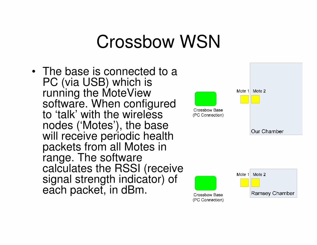
• The base is connected to a PC (via USB) which is running the MoteView software. When configured to ‘talk’ with the wireless nodes (‘Motes’), the base will receive periodic health packets from all Motes in range. The software calculates the RSSI (receive signal strength indicator) of each packet, in dBm.

Crossbow WSN

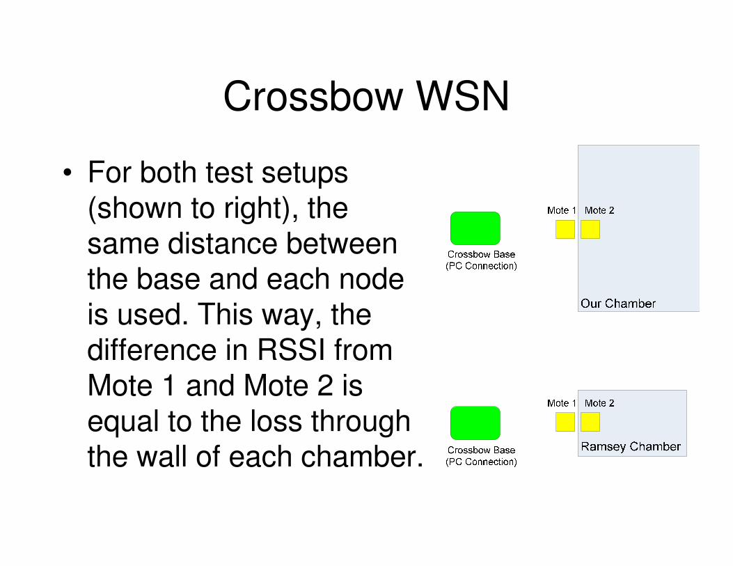
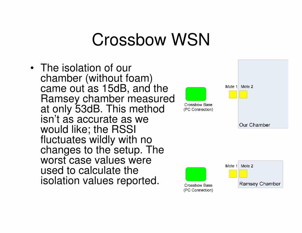
• For both test setups (shown to right), the same distance between the base and each node is used. This way, the difference in RSSI from Mote 1 and Mote 2 is equal to the loss through the wall of each chamber.

Crossbow WSN

• The isolation of our chamber (without foam) came out as 15dB, and the Ramsey chamber measured at only 53dB. This method isn’t as accurate as we would like; the RSSI fluctuates wildly with no changes to the setup. The worst case values were used to calculate the isolation values reported.

Atheros Wi-Fi Module

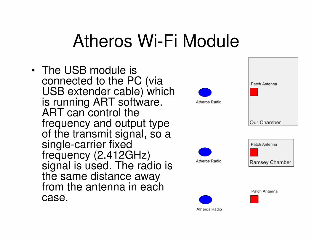
• The USB module is connected to the PC (via USB extender cable) which is running ART software. ART can control the frequency and output type of the transmit signal, so a single-carrier fixed frequency (2.412GHz) signal is used. The radio is the same distance away from the antenna in each case.

Atheros Wi-Fi Module

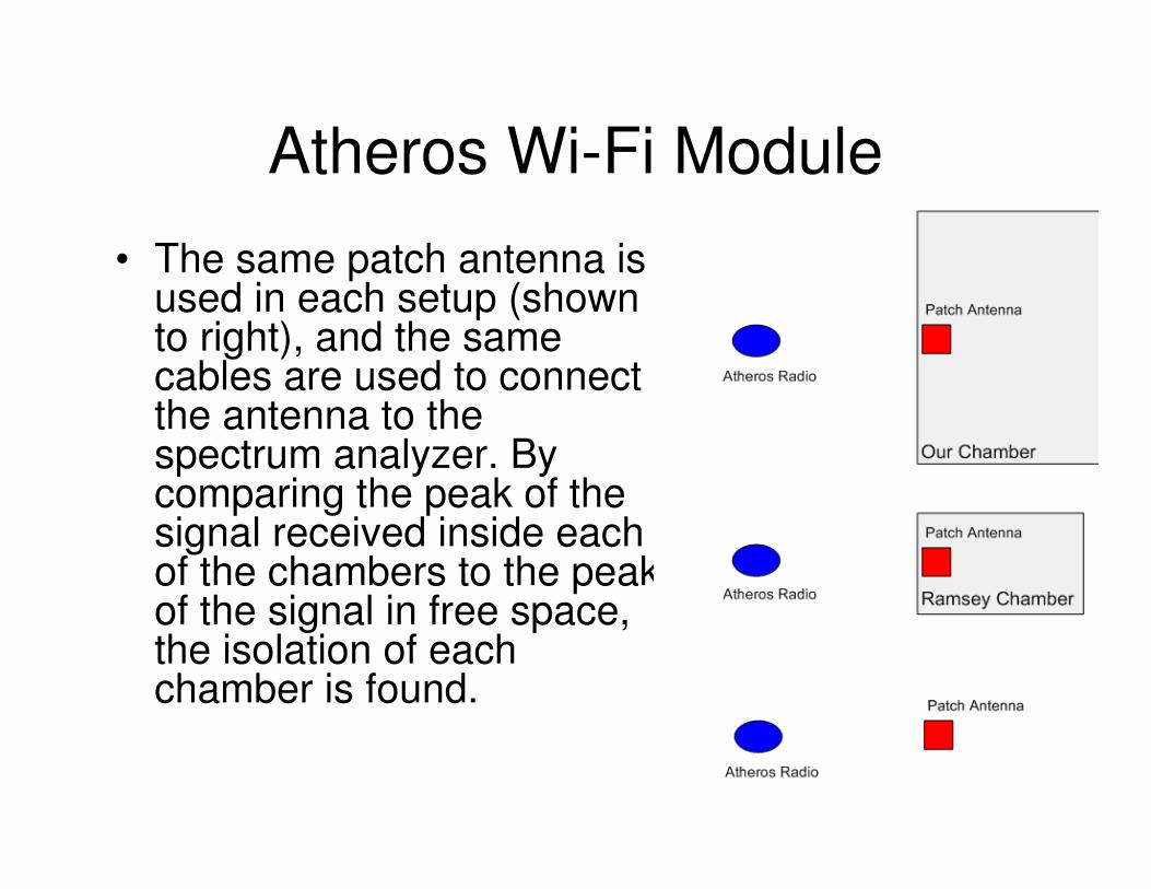
• The same patch antenna is used in each setup (shown to right), and the same cables are used to connect the antenna to the spectrum analyzer. By comparing the peak of the signal received inside each of the chambers to the peak of the signal in free space, the isolation of each chamber is found.

Atheros Wi-Fi Module

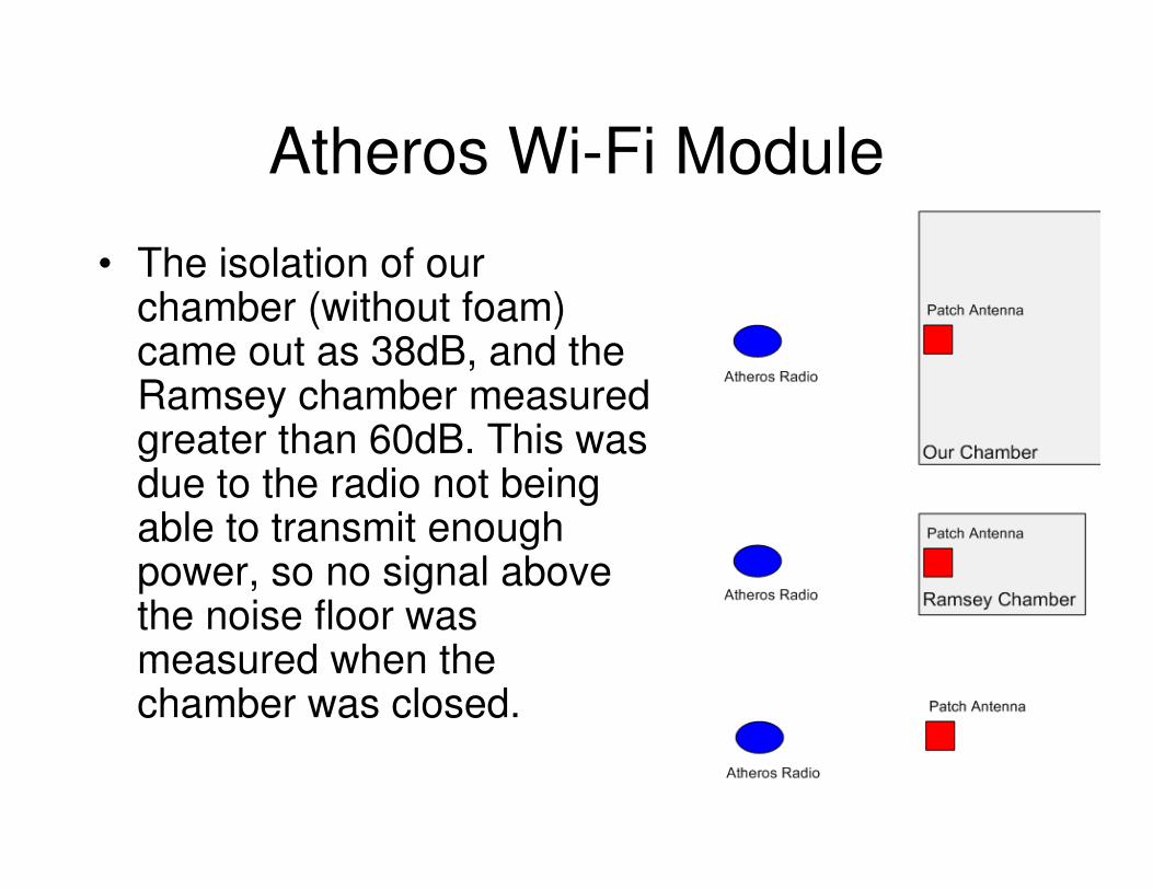
• The isolation of our chamber (without foam) came out as 38dB, and the Ramsey chamber measured greater than 60dB. This was due to the radio not being able to transmit enough power, so no signal above the noise floor was measured when the chamber was closed.

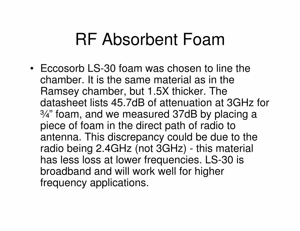
RF Absorbent Foam

• Eccosorb LS-30 foam was chosen to line the chamber. It is the same material as in the Ramsey chamber, but 1.5X thicker. The datasheet lists 45.7dB of attenuation at 3GHz for ¾” foam, and we measured 37dB by placing a piece of foam in the direct path of radio to antenna. This discrepancy could be due to the radio being 2.4GHz (not 3GHz) - this material has less loss at lower frequencies. LS-30 is broadband and will work well for higher frequency applications.

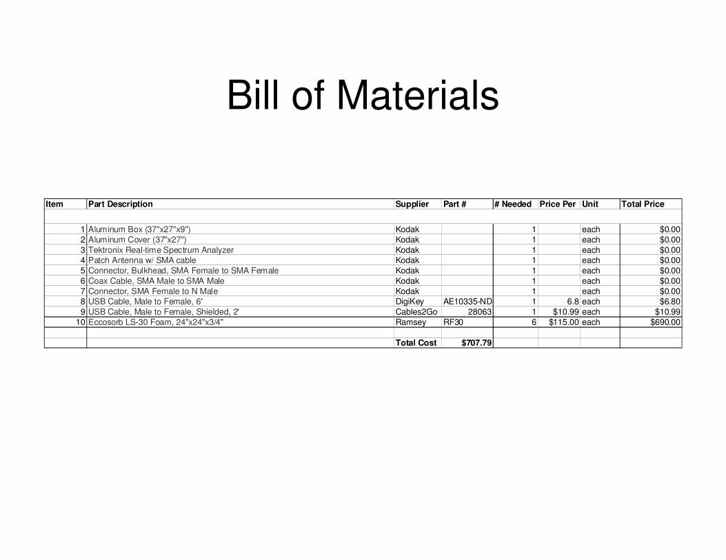
Bill of Materials

Item Part Description Supplier Part # # Needed Price Per Unit Total Price

1 Aluminum Box (37"x27"x9") Kodak 1 each $0.002 Aluminum Cover (37"x27") Kodak 1 each $0.003 Tektronix Real-time Spectrum Analyzer Kodak 1 each $0.004 Patch Antenna w/ SMA cable Kodak 1 each $0.005 Connector, Bulkhead, SMA Female to SMA Female Kodak 1 each $0.006 Coax Cable, SMA Male to SMA Male Kodak 1 each $0.007 Connector, SMA Female to N Male Kodak 1 each $0.008 USB Cable, Male to Female, 6' DigiKey AE10335-ND 1 6.8 each $6.809 USB Cable, Male to Female, Shielded, 2' Cables2Go 28063 1 $10.99 each $10.99

10 Eccosorb LS-30 Foam, 24"x24"x3/4" Ramsey RF30 6 $115.00 each $690.00

Total Cost $707.79

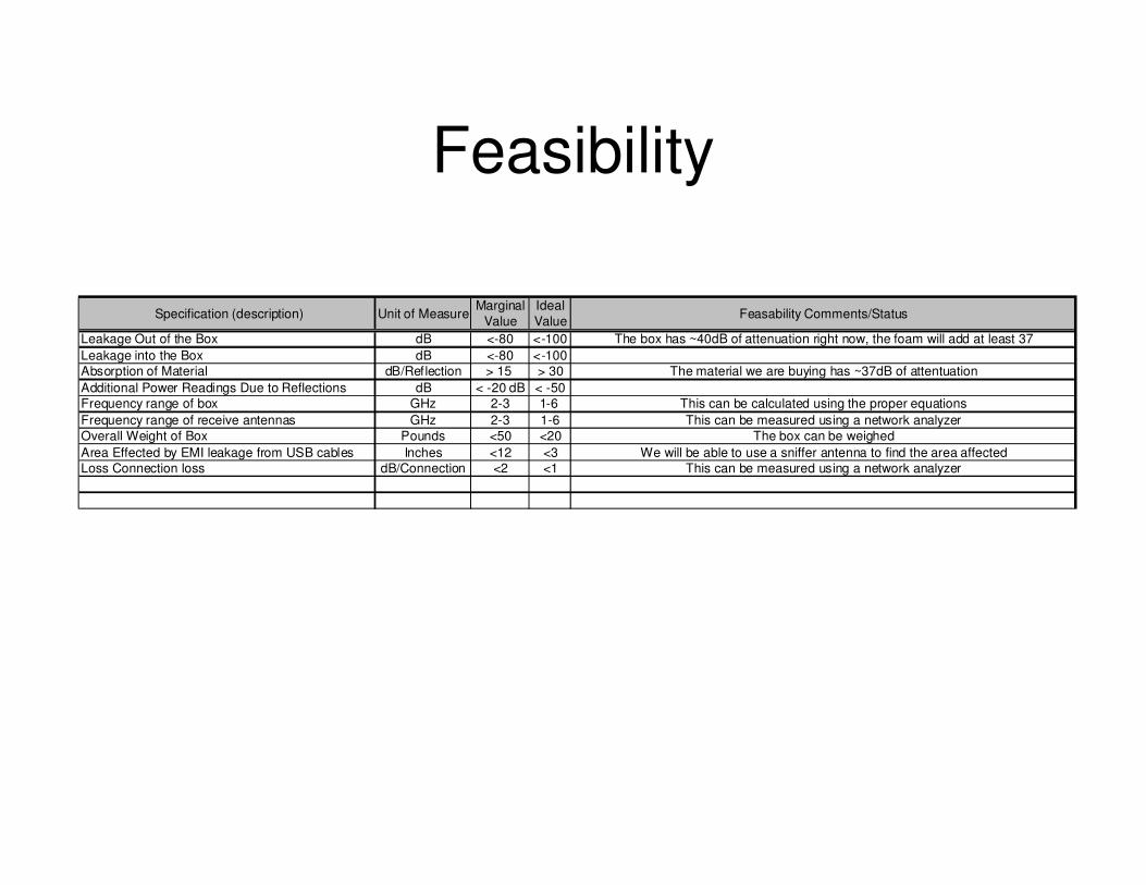
Feasibility

Specification (description) Unit of MeasureMarginal

ValueIdeal Value Feasability Comments/Status

Leakage Out of the Box dB <-80 <-100 The box has ~40dB of attenuation right now, the foam will add at least 37Leakage into the Box dB <-80 <-100Absorption of Material dB/Reflection > 15 > 30 The material we are buying has ~37dB of attentuationAdditional Power Readings Due to Reflections dB < -20 dB < -50Frequency range of box GHz 2-3 1-6 This can be calculated using the proper equationsFrequency range of receive antennas GHz 2-3 1-6 This can be measured using a network analyzerOverall Weight of Box Pounds <50 <20 The box can be weighedArea Effected by EMI leakage from USB cables Inches <12 <3 We will be able to use a sniffer antenna to find the area affectedLoss Connection loss dB/Connection <2 <1 This can be measured using a network analyzer

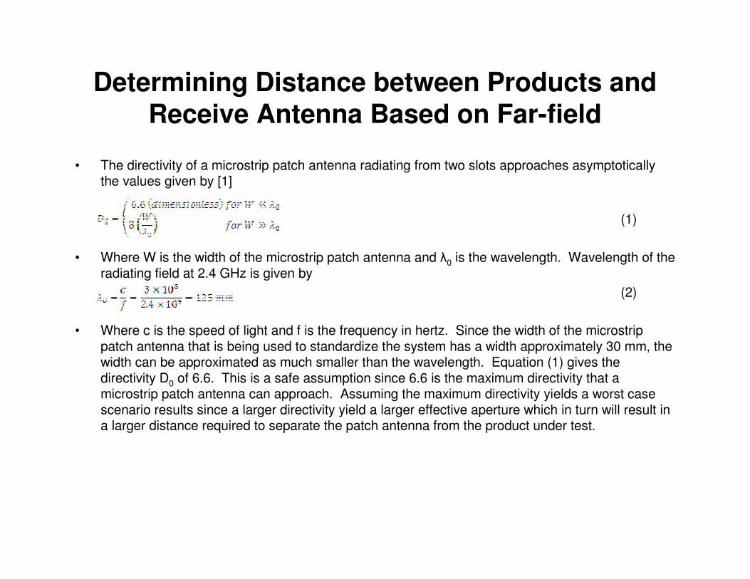
Determining Distance between Products and Receive Antenna Based on Far-field

• The directivity of a microstrip patch antenna radiating from two slots approaches asymptotically the values given by [1]

(1)

• Where W is the width of the microstrip patch antenna and �0 is the wavelength. Wavelength of the radiating field at 2.4 GHz is given by

(2)

• Where c is the speed of light and f is the frequency in hertz. Since the width of the microstrip patch antenna that is being used to standardize the system has a width approximately 30 mm, the width can be approximated as much smaller than the wavelength. Equation (1) gives the directivity D0 of 6.6. This is a safe assumption since 6.6 is the maximum directivity that a microstrip patch antenna can approach. Assuming the maximum directivity yields a worst case scenario results since a larger directivity yield a larger effective aperture which in turn will result in a larger distance required to separate the patch antenna from the product under test.

Determining Distance between Products and Receive Antenna Based on Far-field (cont.)

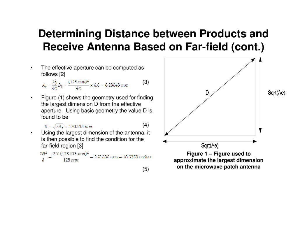
• The effective aperture can be computed as follows [2]

(3)

• Figure (1) shows the geometry used for finding the largest dimension D from the effective aperture. Using basic geometry the value D is found to be

(4)• Using the largest dimension of the antenna, it

is then possible to find the condition for the far-field region [3]

(5)

Figure 1 – Figure used to approximate the largest dimension on the microwave patch antenna

Determining Distance between Products and Receive Antenna Based on Far-field (cont.)

• It is also fairly simple to find the far-field region for a dipole antenna. The equation is given by [4](6)

• Since most of the products that the chamber will be used to test will have an antenna with dimensions between that of a microstrip and that of a dipole antenna, it can be assumed that the antennas with the largest condition for far-field will be patch antennas. Doubling the far-field of the patch antenna gives a distance of approximately 21 inches. This will be the distance used to separate the two antennas. Although it is possible to move the antennas a larger distance away from each other since the chamber is in fact 37 inches in length, another condition prevents this possibility as will be shown in the next section.

• The equations shown and derived here were done assuming that the frequency of test is 2.4 GHz. The goal of the project was to possibly expand the frequency range of 1-6 GHz. For frequencies above 2.4 GHz, a distance of 21 inches should suffice, however, for frequencies below 2.4 GHz, an attenuator should be used to simulate the far-field region as discussed in earlier talks about additions to the project.

Condition for Preventing Skipping Waves

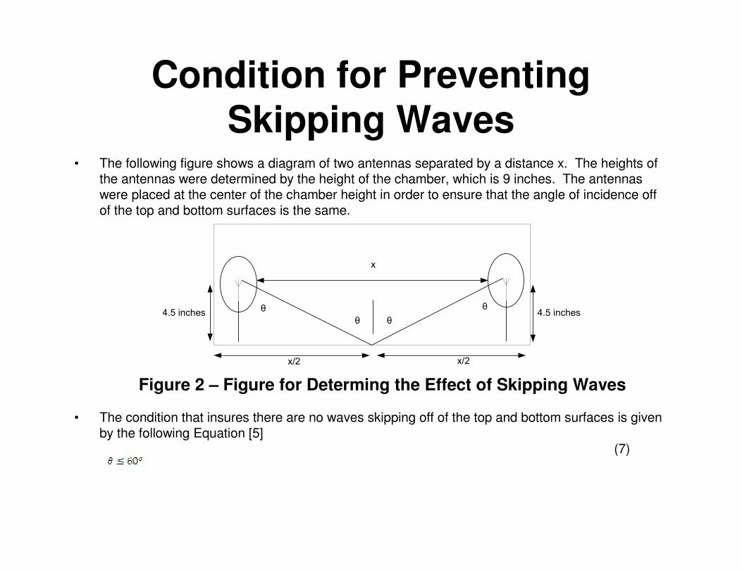
• The following figure shows a diagram of two antennas separated by a distance x. The heights of the antennas were determined by the height of the chamber, which is 9 inches. The antennas were placed at the center of the chamber height in order to ensure that the angle of incidence off of the top and bottom surfaces is the same.

• The condition that insures there are no waves skipping off of the top and bottom surfaces is given by the following Equation [5]

(7)

�

�������� ��������

������

Figure 2 – Figure for Determing the Effect of Skipping Waves

Condition for Preventing Skipping Waves (Cont.)

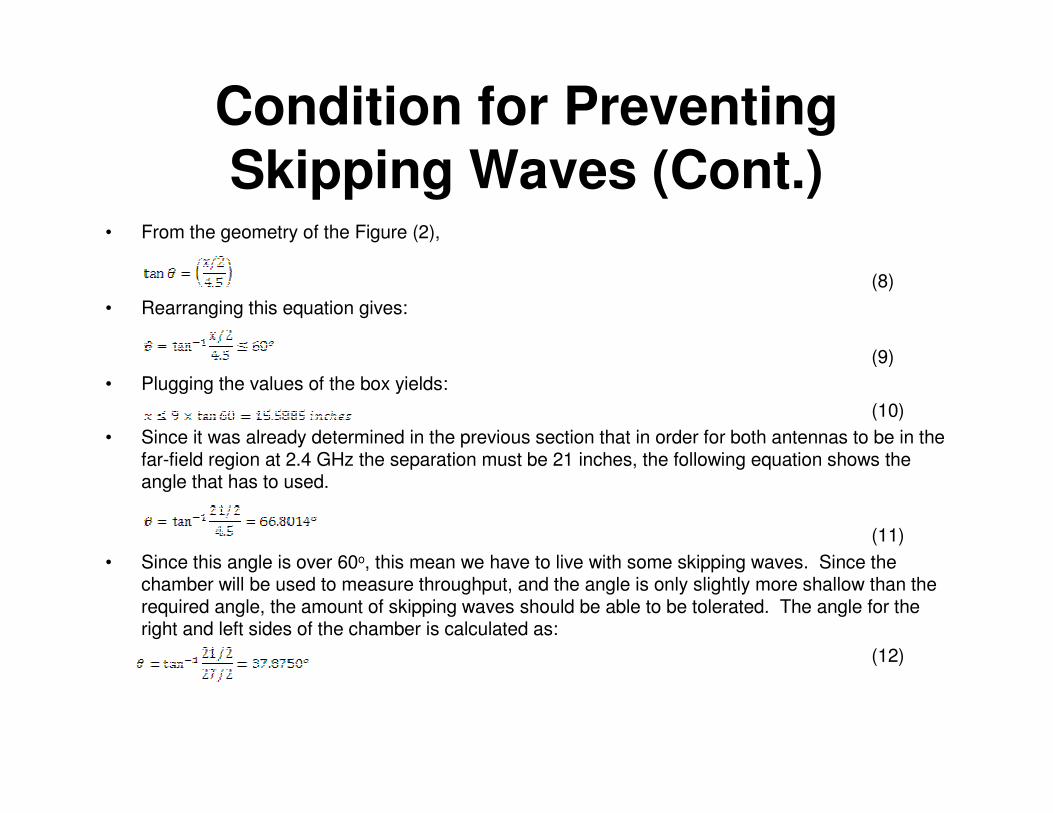
• From the geometry of the Figure (2),

(8)• Rearranging this equation gives:

(9)• Plugging the values of the box yields:

(10)• Since it was already determined in the previous section that in order for both antennas to be in the

far-field region at 2.4 GHz the separation must be 21 inches, the following equation shows the angle that has to used.

(11)• Since this angle is over 60o, this mean we have to live with some skipping waves. Since the

chamber will be used to measure throughput, and the angle is only slightly more shallow than the required angle, the amount of skipping waves should be able to be tolerated. The angle for the right and left sides of the chamber is calculated as:

(12)

Derivation of Specular Regions

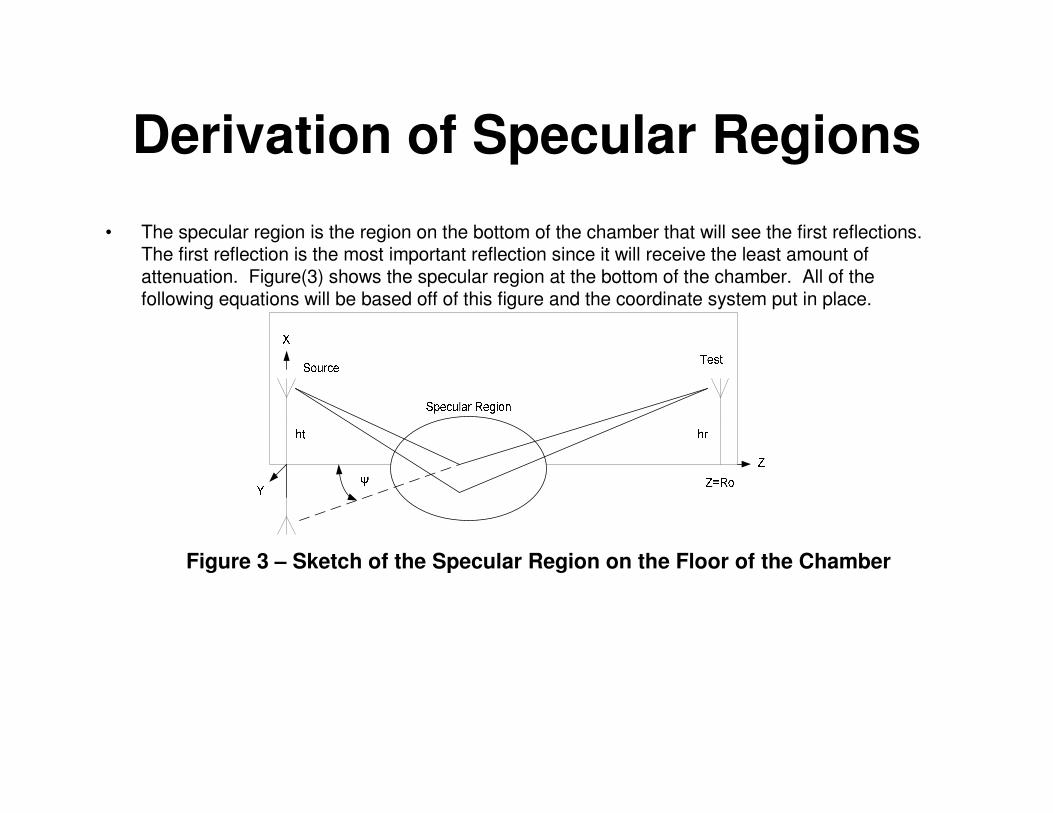
• The specular region is the region on the bottom of the chamber that will see the first reflections. The first reflection is the most important reflection since it will receive the least amount of attenuation. Figure(3) shows the specular region at the bottom of the chamber. All of the following equations will be based off of this figure and the coordinate system put in place.

Figure 3 – Sketch of the Specular Region on the Floor of the Chamber

Derivation of Specular Regions (Cont.)

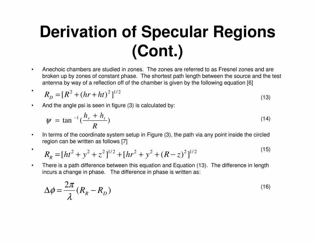
• Anechoic chambers are studied in zones. The zones are referred to as Fresnel zones and are broken up by zones of constant phase. The shortest path length between the source and the test antenna by way of a reflection off of the chamber is given by the following equation [6]

•(13)

• And the angle psi is seen in figure (3) is calculated by:

(14)

• In terms of the coordinate system setup in Figure (3), the path via any point inside the circled region can be written as follows [7]

• (15)

• There is a path difference between this equation and Equation (13). The difference in length incurs a change in phase. The difference in phase is written as:

(16)

2/122 ])([ hthrRRD ++=

)(tan 1

Rhh tr += −ψ

2/12222/1222 ])([][ zRyhrzyhtRR −+++++=

)(2

DR RR −=∆λπφ

Derivation of Specular Regions (Cont.)

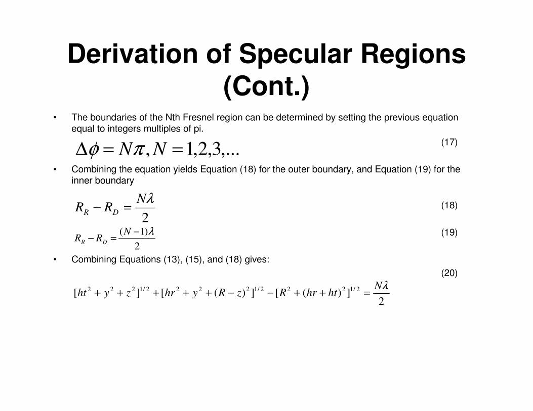
• The boundaries of the Nth Fresnel region can be determined by setting the previous equation equal to integers multiples of pi.

(17)

• Combining the equation yields Equation (18) for the outer boundary, and Equation (19) for the inner boundary

(18)

(19)

• Combining Equations (13), (15), and (18) gives:(20)

,...3,2,1, ==∆ NNπφ

2λN

RR DR =−

2)1( λ−=− N

RR DR

2])([])([][ 2/1222/12222/1222 λN

hthrRzRyhrzyht =++−−+++++

Derivation of Specular Regions (Cont.)

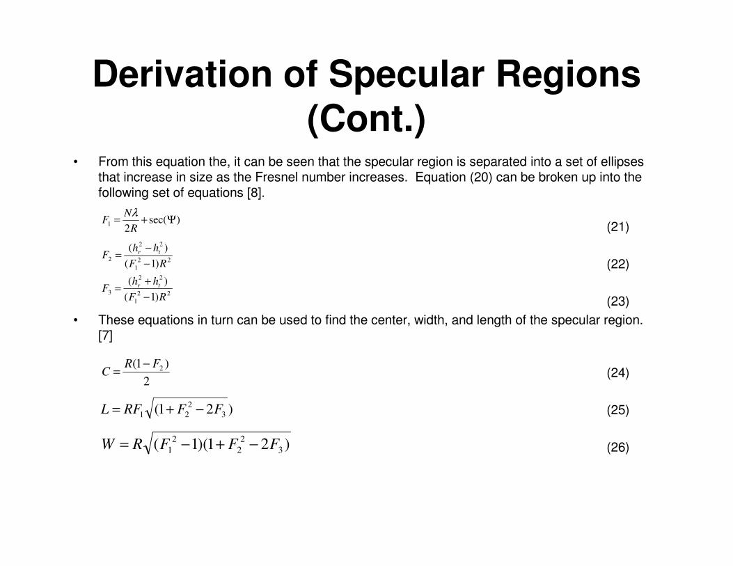
• From this equation the, it can be seen that the specular region is separated into a set of ellipses that increase in size as the Fresnel number increases. Equation (20) can be broken up into the following set of equations [8].

(21)

(22)

(23)• These equations in turn can be used to find the center, width, and length of the specular region.

[7]

(24)

(25)

(26)

)sec(21 Ψ+=

RN

Fλ

221

22

2 )1()(

RFhh

F tr

−−=

221

22

3 )1()(

RFhh

F tr

−+=

2)1( 2FR

C−=

)21( 32

21 FFRFL −+=

)21)(1( 32

22

1 FFFRW −+−=

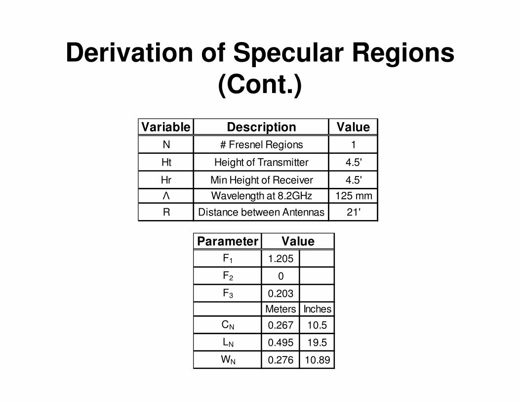
Derivation of Specular Regions (Cont.)

Variable Description ValueN # Fresnel Regions 1

Ht Height of Transmitter 4.5'

Hr Min Height of Receiver 4.5'� Wavelength at 8.2GHz 125 mm

R Distance between Antennas 21'

ParameterF1 1.205

F2 0

F3 0.203Meters Inches

CN 0.267 10.5

LN 0.495 19.5

WN 0.276 10.89

Value

Derivation of Specular Regions (Cont.)

• These equations were derived using ray tracing techniques which are known to only approximate the behavior in the frequency range used here, however, these equations useful for their guidance when considering the reflections in the specular region.

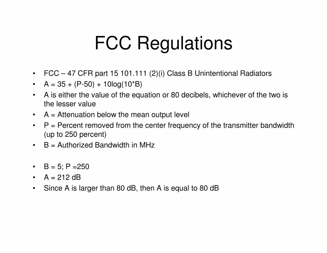
FCC Regulations• FCC – 47 CFR part 15 101.111 (2)(i) Class B Unintentional Radiators• A = 35 + (P-50) + 10log(10*B)• A is either the value of the equation or 80 decibels, whichever of the two is

the lesser value• A = Attenuation below the mean output level• P = Percent removed from the center frequency of the transmitter bandwidth

(up to 250 percent)• B = Authorized Bandwidth in MHz

• B = 5; P =250• A = 212 dB• Since A is larger than 80 dB, then A is equal to 80 dB

References• [1] Constantine A. Balanis, Antenna Theory Third Edition, Hoboken, NJ: John Wiley & Sons,

2005. P.842• [2] Constantine A. Balanis, Antenna Theory Third Edition, Hoboken, NJ: John Wiley & Sons,

2005. P.93• [3] Constantine A. Balanis, Antenna Theory Third Edition, Hoboken, NJ: John Wiley & Sons,

2005. P.170• [4] David M. Pozar, Microwave Engineering Third Edition, Hoboken, NJ: John Wiley & Sons,

2005. p. 636• [5] Leland H. Hemming. Electromagnetic Anechoic Chambers A Fundamental Design and

Specification Guide. Piscataway, NJ: IEEE Press, 2002. p. 74.• [6] Leland H. Hemming. Electromagnetic Anechoic Chambers A Fundamental Design and

Specification Guide. Piscataway, NJ: IEEE Press, 2002. p. 181• [7] Leland H. Hemming. Electromagnetic Anechoic Chambers A Fundamental Design and

Specification Guide. Piscataway, NJ: IEEE Press, 2002. p. 182• [8] Leland H. Hemming. Electromagnetic Anechoic Chambers A Fundamental Design and

Specification Guide. Piscataway, NJ: IEEE Press, 2002. p. 183