Embed Size (px)
Citation preview
Revision Lecture 3:Frequency Responses
Revision Lecture 3:FrequencyResponses
• Frequency Responses
• Plotting FrequencyResponses
• LF and HF Asymptotes
• Corner frequencies (linearfactors)
• Sketching MagnitudeResponses (linear factors)
• Sketching Phase response
• Phase Response Example
• Filters
• Resonance
E1.1 Analysis of Circuits (2015-6186) Revision Lecture 3 – 1 / 10

Frequency Responses
Revision Lecture 3:FrequencyResponses
• Frequency Responses
• Plotting FrequencyResponses
• LF and HF Asymptotes
• Corner frequencies (linearfactors)
• Sketching MagnitudeResponses (linear factors)
• Sketching Phase response
• Phase Response Example
• Filters
• Resonance
E1.1 Analysis of Circuits (2015-6186) Revision Lecture 3 – 2 / 10
• Frequency response is the ratio of two voltage/current phasors in acircuit: output phasor ÷ input phasor.
◦ It is a complex number that depends on frequency.
◦ Calculate using nodal analysis.
• For a linear circuit, the frequency response is always a ratio of twopolynomials in jω having real coefficients that depend on thecomponent values.
YX = R+1/jωC
4R+1/jωC= jωRC+1
jω4RC+1

Plotting Frequency Responses
Revision Lecture 3:FrequencyResponses
• Frequency Responses
• Plotting FrequencyResponses
• LF and HF Asymptotes
• Corner frequencies (linearfactors)
• Sketching MagnitudeResponses (linear factors)
• Sketching Phase response
• Phase Response Example
• Filters
• Resonance
E1.1 Analysis of Circuits (2015-6186) Revision Lecture 3 – 3 / 10
• Plot the magnitude response and phase response as separate graphs.Use log scale for frequency and magnitude and linear scale for phase:this gives graphs that can be approximated by straight line segments.
• If V2
V1
= A (jω)k = A× jk × ωk
◦ magnitude is a straight line with gradient k:
log∣
∣
∣
V2
V1
∣
∣
∣= log |A|+ k logω
◦ phase is a constant k × π2 (+π if A < 0):
∠
(
V2
V1
)
= ∠A+ k∠j = ∠A+ k π2
• Measure magnitude using decibels = 20 log10|V2||V1| .
A gradient of k on log axes is the same as a gradient of 20k dB/decade(×10 in frequency) or 6k dB/octave ( ×2 in frequency).
YX =
1
jωC
R+ 1
jωC
= 1jωRC+1

Plotting Frequency Responses
Revision Lecture 3:FrequencyResponses
• Frequency Responses
• Plotting FrequencyResponses
• LF and HF Asymptotes
• Corner frequencies (linearfactors)
• Sketching MagnitudeResponses (linear factors)
• Sketching Phase response
• Phase Response Example
• Filters
• Resonance
E1.1 Analysis of Circuits (2015-6186) Revision Lecture 3 – 3 / 10
• Plot the magnitude response and phase response as separate graphs.Use log scale for frequency and magnitude and linear scale for phase:this gives graphs that can be approximated by straight line segments.
• If V2
V1
= A (jω)k = A× jk × ωk
◦ magnitude is a straight line with gradient k:
log∣
∣
∣
V2
V1
∣
∣
∣= log |A|+ k logω
◦ phase is a constant k × π2 (+π if A < 0):
∠
(
V2
V1
)
= ∠A+ k∠j = ∠A+ k π2
• Measure magnitude using decibels = 20 log10|V2||V1| .
A gradient of k on log axes is the same as a gradient of 20k dB/decade(×10 in frequency) or 6k dB/octave ( ×2 in frequency).
0.1/RC 1/RC 10/RC-30
-20
-10
0
ω (rad/s)
|Gai
n| (
dB)
0.1/RC 1/RC 10/RC
-0.4
-0.2
0
ω (rad/s)
Pha
se/π
YX =
1
jωC
R+ 1
jωC
= 1jωRC+1=
1jωωc
+1where ωc =
1RC

LF and HF Asymptotes
Revision Lecture 3:FrequencyResponses
• Frequency Responses
• Plotting FrequencyResponses
• LF and HF Asymptotes
• Corner frequencies (linearfactors)
• Sketching MagnitudeResponses (linear factors)
• Sketching Phase response
• Phase Response Example
• Filters
• Resonance
E1.1 Analysis of Circuits (2015-6186) Revision Lecture 3 – 4 / 10
• Frequency response is always a ratio of two polynomials in jω withreal coefficients that depend on the component values.
◦ The terms with the lowest power of jω on top and bottom givesthe low-frequency asymptote
◦ The terms with the highest power of jω on top and bottomgives the high-frequency asymptote.
Example: H(jω) = 60(jω)2+720(jω)
3(jω)3+165(jω)2+762(jω)+600
0.1 1 10 100 1000
-40
-20
0
ω (rad/s)0.1 1 10 100 1000
-0.5
0
0.5
ω (rad/s)
π

LF and HF Asymptotes
Revision Lecture 3:FrequencyResponses
• Frequency Responses
• Plotting FrequencyResponses
• LF and HF Asymptotes
• Corner frequencies (linearfactors)
• Sketching MagnitudeResponses (linear factors)
• Sketching Phase response
• Phase Response Example
• Filters
• Resonance
E1.1 Analysis of Circuits (2015-6186) Revision Lecture 3 – 4 / 10
• Frequency response is always a ratio of two polynomials in jω withreal coefficients that depend on the component values.
◦ The terms with the lowest power of jω on top and bottom givesthe low-frequency asymptote
◦ The terms with the highest power of jω on top and bottomgives the high-frequency asymptote.
Example: H(jω) = 60(jω)2+720(jω)
3(jω)3+165(jω)2+762(jω)+600
0.1 1 10 100 1000
-40
-20
0
ω (rad/s)0.1 1 10 100 1000
-0.5
0
0.5
ω (rad/s)
πLF: H(jω) ≃ 1.2jω
HF: H(jω) ≃ 20 (jω)−1

Corner frequencies (linear factors)
Revision Lecture 3:FrequencyResponses
• Frequency Responses
• Plotting FrequencyResponses
• LF and HF Asymptotes
• Corner frequencies (linearfactors)
• Sketching MagnitudeResponses (linear factors)
• Sketching Phase response
• Phase Response Example
• Filters
• Resonance
E1.1 Analysis of Circuits (2015-6186) Revision Lecture 3 – 5 / 10
• We can factorize the numerator and denominator into linear terms of
the form (ajω + b) ≃
{
b ω <∣
∣
ba
∣
∣
ajω ω >∣
∣
ba
∣
∣
.
• At the corner frequency, ωc =∣
∣
ba
∣
∣ the slope of the magnituderesponse changes by ±1 ( ≡ ±20 dB/decade) because the linearterm introduces another factor of ω into the numerator ordenominator for ω > ωc.
• The phase changes by ±π2 because the linear term introduces
another factor of j into the numerator or denominator for ω > ωc.
◦ The phase change is gradual and takes place over the range0.1ωc to 10ωc (±π
2 spread over two decades in ω).
• When a and b are real and positive, it is often convenient to write
(ajω + b) = b(
jωωc
+ 1)
.
• The corner frequencies are the absolute values of the roots (valuesof jω) of the numerator and denominator polynomials.

Sketching Magnitude Responses (linear factors)
Revision Lecture 3:FrequencyResponses
• Frequency Responses
• Plotting FrequencyResponses
• LF and HF Asymptotes
• Corner frequencies (linearfactors)
• Sketching MagnitudeResponses (linear factors)
• Sketching Phase response
• Phase Response Example
• Filters
• Resonance
E1.1 Analysis of Circuits (2015-6186) Revision Lecture 3 – 6 / 10
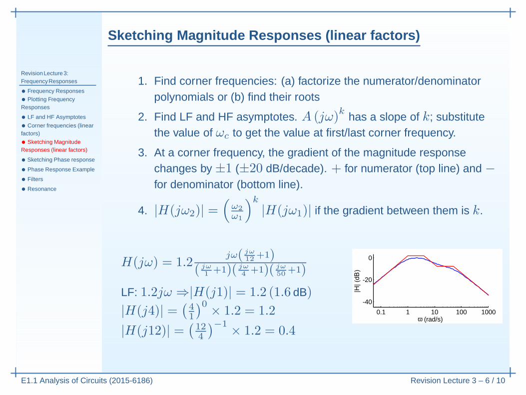
1. Find corner frequencies: (a) factorize the numerator/denominatorpolynomials or (b) find their roots
2. Find LF and HF asymptotes. A (jω)k
has a slope of k; substitutethe value of ωc to get the value at first/last corner frequency.
3. At a corner frequency, the gradient of the magnitude responsechanges by ±1 (±20 dB/decade). + for numerator (top line) and −for denominator (bottom line).
4. |H(jω2)| =(
ω2
ω1
)k
|H(jω1)| if the gradient between them is k.

Sketching Magnitude Responses (linear factors)
Revision Lecture 3:FrequencyResponses
• Frequency Responses
• Plotting FrequencyResponses
• LF and HF Asymptotes
• Corner frequencies (linearfactors)
• Sketching MagnitudeResponses (linear factors)
• Sketching Phase response
• Phase Response Example
• Filters
• Resonance
E1.1 Analysis of Circuits (2015-6186) Revision Lecture 3 – 6 / 10
1. Find corner frequencies: (a) factorize the numerator/denominatorpolynomials or (b) find their roots
2. Find LF and HF asymptotes. A (jω)k
has a slope of k; substitutethe value of ωc to get the value at first/last corner frequency.
3. At a corner frequency, the gradient of the magnitude responsechanges by ±1 (±20 dB/decade). + for numerator (top line) and −for denominator (bottom line).
4. |H(jω2)| =(
ω2
ω1
)k
|H(jω1)| if the gradient between them is k.
H(jω) = 1.2jω( jω
12+1)
( jω1+1)( jω
4+1)( jω
50+1)
0.1 1 10 100 1000
-40
-20
0
ω (rad/s)

Sketching Magnitude Responses (linear factors)
Revision Lecture 3:FrequencyResponses
• Frequency Responses
• Plotting FrequencyResponses
• LF and HF Asymptotes
• Corner frequencies (linearfactors)
• Sketching MagnitudeResponses (linear factors)
• Sketching Phase response
• Phase Response Example
• Filters
• Resonance
E1.1 Analysis of Circuits (2015-6186) Revision Lecture 3 – 6 / 10
1. Find corner frequencies: (a) factorize the numerator/denominatorpolynomials or (b) find their roots
2. Find LF and HF asymptotes. A (jω)k
has a slope of k; substitutethe value of ωc to get the value at first/last corner frequency.
3. At a corner frequency, the gradient of the magnitude responsechanges by ±1 (±20 dB/decade). + for numerator (top line) and −for denominator (bottom line).
4. |H(jω2)| =(
ω2
ω1
)k
|H(jω1)| if the gradient between them is k.
H(jω) = 1.2jω( jω
12+1)
( jω1+1)( jω
4+1)( jω
50+1)
LF: 1.2jω ⇒|H(j1)| = 1.2 (1.6 dB)
|H(j4)| =(
41
)0× 1.2 = 1.2 0.1 1 10 100 1000
-40
-20
0
ω (rad/s)
Sketching Magnitude Responses (linear factors)
Revision Lecture 3:FrequencyResponses
• Frequency Responses
• Plotting FrequencyResponses
• LF and HF Asymptotes
• Corner frequencies (linearfactors)
• Sketching MagnitudeResponses (linear factors)
• Sketching Phase response
• Phase Response Example
• Filters
• Resonance
E1.1 Analysis of Circuits (2015-6186) Revision Lecture 3 – 6 / 10
1. Find corner frequencies: (a) factorize the numerator/denominatorpolynomials or (b) find their roots
2. Find LF and HF asymptotes. A (jω)k
has a slope of k; substitutethe value of ωc to get the value at first/last corner frequency.
3. At a corner frequency, the gradient of the magnitude responsechanges by ±1 (±20 dB/decade). + for numerator (top line) and −for denominator (bottom line).
4. |H(jω2)| =(
ω2
ω1
)k
|H(jω1)| if the gradient between them is k.
H(jω) = 1.2jω( jω
12+1)
( jω1+1)( jω
4+1)( jω
50+1)
LF: 1.2jω ⇒|H(j1)| = 1.2 (1.6 dB)
|H(j4)| =(
41
)0× 1.2 = 1.2
|H(j12)| =(
124
)−1× 1.2 = 0.4
0.1 1 10 100 1000
-40
-20
0
ω (rad/s)

Sketching Magnitude Responses (linear factors)
Revision Lecture 3:FrequencyResponses
• Frequency Responses
• Plotting FrequencyResponses
• LF and HF Asymptotes
• Corner frequencies (linearfactors)
• Sketching MagnitudeResponses (linear factors)
• Sketching Phase response
• Phase Response Example
• Filters
• Resonance
E1.1 Analysis of Circuits (2015-6186) Revision Lecture 3 – 6 / 10
1. Find corner frequencies: (a) factorize the numerator/denominatorpolynomials or (b) find their roots
2. Find LF and HF asymptotes. A (jω)k
has a slope of k; substitutethe value of ωc to get the value at first/last corner frequency.
3. At a corner frequency, the gradient of the magnitude responsechanges by ±1 (±20 dB/decade). + for numerator (top line) and −for denominator (bottom line).
4. |H(jω2)| =(
ω2
ω1
)k
|H(jω1)| if the gradient between them is k.
H(jω) = 1.2jω( jω
12+1)
( jω1+1)( jω
4+1)( jω
50+1)
LF: 1.2jω ⇒|H(j1)| = 1.2 (1.6 dB)
|H(j4)| =(
41
)0× 1.2 = 1.2
|H(j12)| =(
124
)−1× 1.2 = 0.4
0.1 1 10 100 1000
-40
-20
0
ω (rad/s)
|H(j50)| =(
5012
)0× 0.4 = 0.4 (−8 dB).

Sketching Magnitude Responses (linear factors)
Revision Lecture 3:FrequencyResponses
• Frequency Responses
• Plotting FrequencyResponses
• LF and HF Asymptotes
• Corner frequencies (linearfactors)
• Sketching MagnitudeResponses (linear factors)
• Sketching Phase response
• Phase Response Example
• Filters
• Resonance
E1.1 Analysis of Circuits (2015-6186) Revision Lecture 3 – 6 / 10
1. Find corner frequencies: (a) factorize the numerator/denominatorpolynomials or (b) find their roots
2. Find LF and HF asymptotes. A (jω)k
has a slope of k; substitutethe value of ωc to get the value at first/last corner frequency.
3. At a corner frequency, the gradient of the magnitude responsechanges by ±1 (±20 dB/decade). + for numerator (top line) and −for denominator (bottom line).
4. |H(jω2)| =(
ω2
ω1
)k
|H(jω1)| if the gradient between them is k.
H(jω) = 1.2jω( jω
12+1)
( jω1+1)( jω
4+1)( jω
50+1)
LF: 1.2jω ⇒|H(j1)| = 1.2 (1.6 dB)
|H(j4)| =(
41
)0× 1.2 = 1.2
|H(j12)| =(
124
)−1× 1.2 = 0.4
0.1 1 10 100 1000
-40
-20
0
ω (rad/s)
|H(j50)| =(
5012
)0× 0.4 = 0.4 (−8 dB). As a check: HF: 20 (jω)−1

Sketching Phase response
Revision Lecture 3:FrequencyResponses
• Frequency Responses
• Plotting FrequencyResponses
• LF and HF Asymptotes
• Corner frequencies (linearfactors)
• Sketching MagnitudeResponses (linear factors)
• Sketching Phase response
• Phase Response Example
• Filters
• Resonance
E1.1 Analysis of Circuits (2015-6186) Revision Lecture 3 – 7 / 10
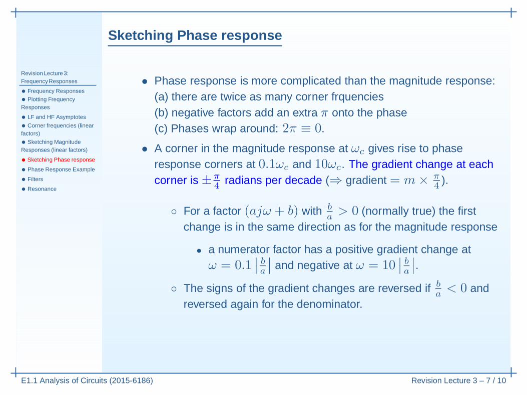
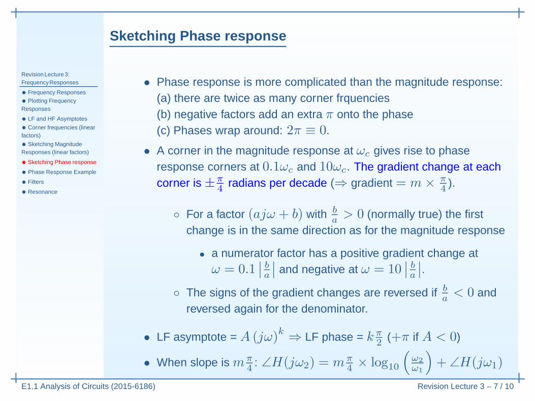
• Phase response is more complicated than the magnitude response:(a) there are twice as many corner frquencies(b) negative factors add an extra π onto the phase(c) Phases wrap around: 2π ≡ 0.

Sketching Phase response
Revision Lecture 3:FrequencyResponses
• Frequency Responses
• Plotting FrequencyResponses
• LF and HF Asymptotes
• Corner frequencies (linearfactors)
• Sketching MagnitudeResponses (linear factors)
• Sketching Phase response
• Phase Response Example
• Filters
• Resonance
E1.1 Analysis of Circuits (2015-6186) Revision Lecture 3 – 7 / 10
• Phase response is more complicated than the magnitude response:(a) there are twice as many corner frquencies(b) negative factors add an extra π onto the phase(c) Phases wrap around: 2π ≡ 0.
• A corner in the magnitude response at ωc gives rise to phaseresponse corners at 0.1ωc and 10ωc. The gradient change at eachcorner is ±π
4 radians per decade (⇒ gradient = m× π4 ).
◦ For a factor (ajω + b) with ba > 0 (normally true) the first
change is in the same direction as for the magnitude response
• a numerator factor has a positive gradient change atω = 0.1
∣
∣
ba
∣
∣ and negative at ω = 10∣
∣
ba
∣
∣.
◦ The signs of the gradient changes are reversed if ba < 0 and
reversed again for the denominator.
• LF asymptote = A (jω)k ⇒ LF phase = k π2 (+π if A < 0)
• When slope is mπ4 : ∠H(jω2) = mπ
4 × log10
(
ω2
ω1
)
+ ∠H(jω1)
Phase Response Example
Revision Lecture 3:FrequencyResponses
• Frequency Responses
• Plotting FrequencyResponses
• LF and HF Asymptotes
• Corner frequencies (linearfactors)
• Sketching MagnitudeResponses (linear factors)
• Sketching Phase response
• Phase Response Example
• Filters
• Resonance
E1.1 Analysis of Circuits (2015-6186) Revision Lecture 3 – 8 / 10
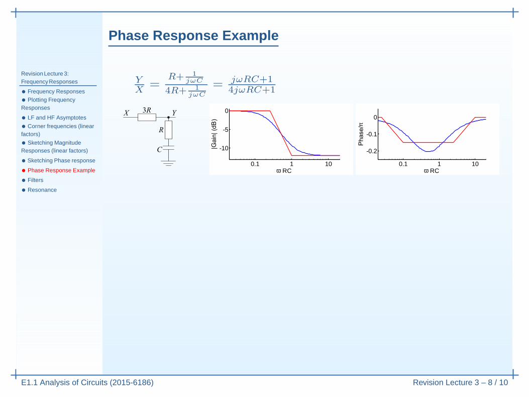
YX =
R+ 1
jωC
4R+ 1
jωC
= jωRC+14jωRC+1
0.1 1 10
-10
-5
0
ω RC0.1 1 10
-0.2
-0.1
0
ω RC
π

Phase Response Example
Revision Lecture 3:FrequencyResponses
• Frequency Responses
• Plotting FrequencyResponses
• LF and HF Asymptotes
• Corner frequencies (linearfactors)
• Sketching MagnitudeResponses (linear factors)
• Sketching Phase response
• Phase Response Example
• Filters
• Resonance
E1.1 Analysis of Circuits (2015-6186) Revision Lecture 3 – 8 / 10
YX =
R+ 1
jωC
4R+ 1
jωC
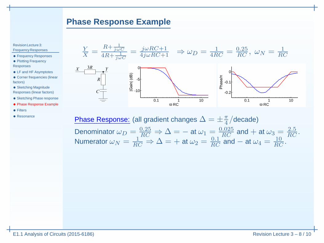
= jωRC+14jωRC+1 ⇒ ωD = 1
4RC = 0.25RC
0.1 1 10
-10
-5
0
ω RC0.1 1 10
-0.2
-0.1
0
ω RC
π
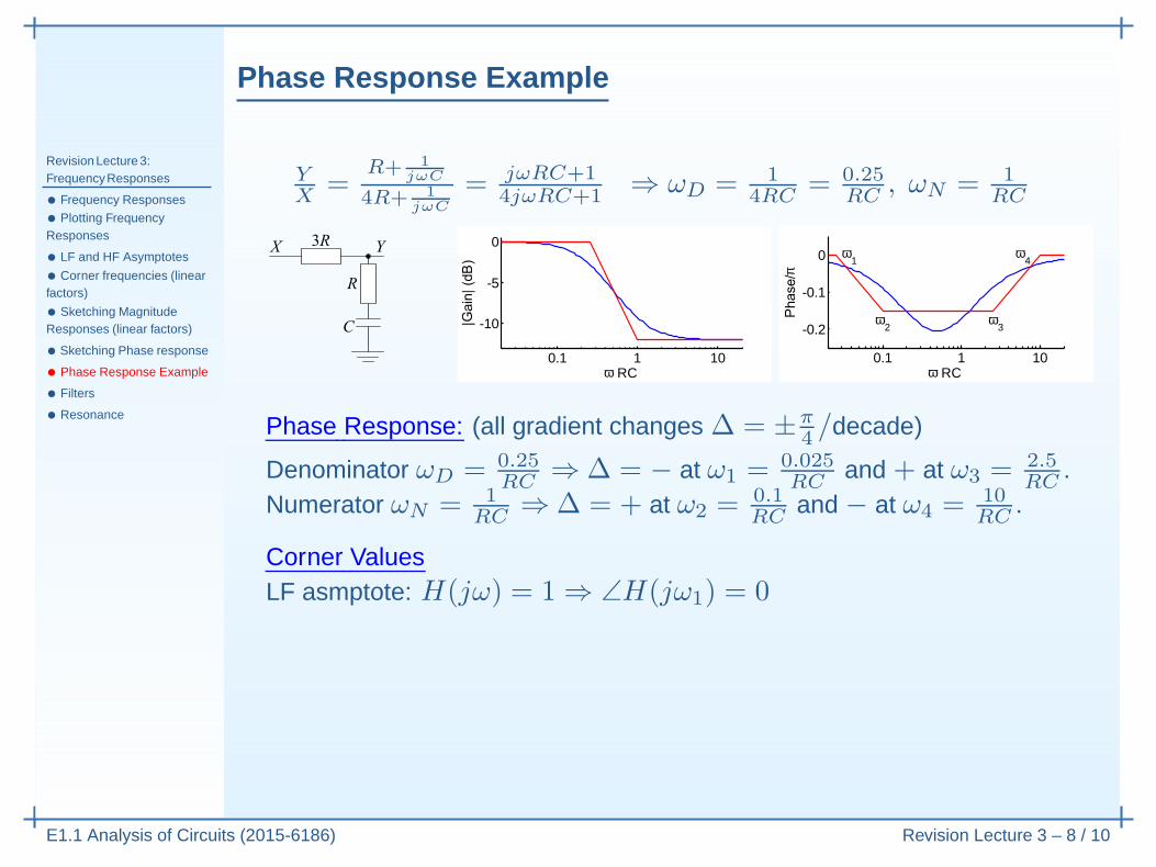
Phase Response: (all gradient changes ∆ = ±π4 /decade)
Denominator ωD = 0.25RC ⇒∆ = − at ω1 = 0.025
RC and + at ω3 = 2.5RC .
Phase Response Example
Revision Lecture 3:FrequencyResponses
• Frequency Responses
• Plotting FrequencyResponses
• LF and HF Asymptotes
• Corner frequencies (linearfactors)
• Sketching MagnitudeResponses (linear factors)
• Sketching Phase response
• Phase Response Example
• Filters
• Resonance
E1.1 Analysis of Circuits (2015-6186) Revision Lecture 3 – 8 / 10
YX =
R+ 1
jωC
4R+ 1
jωC
= jωRC+14jωRC+1 ⇒ ωD = 1
4RC = 0.25RC , ωN = 1
RC
0.1 1 10
-10
-5
0
ω RC0.1 1 10
-0.2
-0.1
0
ω RC
π
Phase Response: (all gradient changes ∆ = ±π4 /decade)
Denominator ωD = 0.25RC ⇒∆ = − at ω1 = 0.025
RC and + at ω3 = 2.5RC .
Numerator ωN = 1RC ⇒∆ = + at ω2 = 0.1
RC and − at ω4 = 10RC .

Phase Response Example
Revision Lecture 3:FrequencyResponses
• Frequency Responses
• Plotting FrequencyResponses
• LF and HF Asymptotes
• Corner frequencies (linearfactors)
• Sketching MagnitudeResponses (linear factors)
• Sketching Phase response
• Phase Response Example
• Filters
• Resonance
E1.1 Analysis of Circuits (2015-6186) Revision Lecture 3 – 8 / 10
YX =
R+ 1
jωC
4R+ 1
jωC
= jωRC+14jωRC+1 ⇒ ωD = 1
4RC = 0.25RC , ωN = 1
RC
0.1 1 10
-10
-5
0
ω RC0.1 1 10
-0.2
-0.1
0
ω RC
π
ω1
ω2
ω3
ω4
Phase Response: (all gradient changes ∆ = ±π4 /decade)
Denominator ωD = 0.25RC ⇒∆ = − at ω1 = 0.025
RC and + at ω3 = 2.5RC .
Numerator ωN = 1RC ⇒∆ = + at ω2 = 0.1
RC and − at ω4 = 10RC .
Corner ValuesLF asmptote: H(jω) = 1 ⇒ ∠H(jω1) = 0
∠H(jω2) = ∠H(jω1)−π4 log10
(
ω2
ω1
)
= −π4 log10 (4) = −0.151π
∠H(jω3) = ∠H(jω2)− 0× log10
(
ω3
ω2
)
= −0.151π
∠H(jω4) = ∠H(jω3) +π4 log10
(
ω4
ω3
)
= −0.151π + π4 log10 (4) = 0

Filters
Revision Lecture 3:FrequencyResponses
• Frequency Responses
• Plotting FrequencyResponses
• LF and HF Asymptotes
• Corner frequencies (linearfactors)
• Sketching MagnitudeResponses (linear factors)
• Sketching Phase response
• Phase Response Example
• Filters
• Resonance
E1.1 Analysis of Circuits (2015-6186) Revision Lecture 3 – 9 / 10
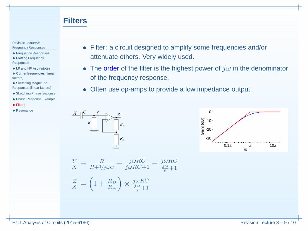
• Filter: a circuit designed to amplify some frequencies and/orattenuate others. Very widely used.
• The order of the filter is the highest power of jω in the denominatorof the frequency response.
• Often use op-amps to provide a low impedance output.

Filters
Revision Lecture 3:FrequencyResponses
• Frequency Responses
• Plotting FrequencyResponses
• LF and HF Asymptotes
• Corner frequencies (linearfactors)
• Sketching MagnitudeResponses (linear factors)
• Sketching Phase response
• Phase Response Example
• Filters
• Resonance
E1.1 Analysis of Circuits (2015-6186) Revision Lecture 3 – 9 / 10
• Filter: a circuit designed to amplify some frequencies and/orattenuate others. Very widely used.
• The order of the filter is the highest power of jω in the denominatorof the frequency response.
• Often use op-amps to provide a low impedance output.
YX = R
R+1/jωC

Filters
Revision Lecture 3:FrequencyResponses
• Frequency Responses
• Plotting FrequencyResponses
• LF and HF Asymptotes
• Corner frequencies (linearfactors)
• Sketching MagnitudeResponses (linear factors)
• Sketching Phase response
• Phase Response Example
• Filters
• Resonance
E1.1 Analysis of Circuits (2015-6186) Revision Lecture 3 – 9 / 10
• Filter: a circuit designed to amplify some frequencies and/orattenuate others. Very widely used.
• The order of the filter is the highest power of jω in the denominatorof the frequency response.
• Often use op-amps to provide a low impedance output.
YX = R
R+1/jωC= jωRC
jωRC+1

Filters
Revision Lecture 3:FrequencyResponses
• Frequency Responses
• Plotting FrequencyResponses
• LF and HF Asymptotes
• Corner frequencies (linearfactors)
• Sketching MagnitudeResponses (linear factors)
• Sketching Phase response
• Phase Response Example
• Filters
• Resonance
E1.1 Analysis of Circuits (2015-6186) Revision Lecture 3 – 9 / 10
• Filter: a circuit designed to amplify some frequencies and/orattenuate others. Very widely used.
• The order of the filter is the highest power of jω in the denominatorof the frequency response.
• Often use op-amps to provide a low impedance output.
YX = R
R+1/jωC= jωRC
jωRC+1 =jωRCjωa
+1

Filters
Revision Lecture 3:FrequencyResponses
• Frequency Responses
• Plotting FrequencyResponses
• LF and HF Asymptotes
• Corner frequencies (linearfactors)
• Sketching MagnitudeResponses (linear factors)
• Sketching Phase response
• Phase Response Example
• Filters
• Resonance
E1.1 Analysis of Circuits (2015-6186) Revision Lecture 3 – 9 / 10
• Filter: a circuit designed to amplify some frequencies and/orattenuate others. Very widely used.
• The order of the filter is the highest power of jω in the denominatorof the frequency response.
• Often use op-amps to provide a low impedance output.
0.1a a 10a
-30
-20
-10
0
ω
YX = R
R+1/jωC= jωRC
jωRC+1 =jωRCjωa
+1
ZX =
(
1 + RB
RA
)
× jωRCjωa
+1
Resonance
E1.1 Analysis of Circuits (2015-6186) Revision Lecture 3 – 10 / 10
• Resonant circuits have quadratic factors that cannot be factorized
◦ H(jω) = a (jω)2 + bjω + c = c
(
(
jωω0
)2
+ 2ζ(
jωω0
)
+ 1
)

Resonance
E1.1 Analysis of Circuits (2015-6186) Revision Lecture 3 – 10 / 10
• Resonant circuits have quadratic factors that cannot be factorized
◦ H(jω) = a (jω)2 + bjω + c = c
(
(
jωω0
)2
+ 2ζ(
jωω0
)
+ 1
)
◦ Resonant frequency: ω0 =√
ca determines the horizontal position
◦ Damping Factor: ζ = bω0
2c = b√4ac
determines the response shape
◦ Equivalently Quality Factor: Q ,ω×Stored EnergyPower Dissipation ≈ 1
2ζ = cbω0
• At ω = ω0, outer terms cancel (a (jω)2= −c): ⇒ H(jω) = jbω0 = 2jcζ
◦ |H(jω0)| = 2ζ times the straight line approximation at ω0.
XU =
1
jωC
R+jωL+ 1
jωC
= 1(jω)2LC+jωRC+1
ω0 =√
1LC , ζ = R
2
√
CL , Q = ω0L
R = 12ζ

Resonance
E1.1 Analysis of Circuits (2015-6186) Revision Lecture 3 – 10 / 10
• Resonant circuits have quadratic factors that cannot be factorized
◦ H(jω) = a (jω)2 + bjω + c = c
(
(
jωω0
)2
+ 2ζ(
jωω0
)
+ 1
)
◦ Resonant frequency: ω0 =√
ca determines the horizontal position
◦ Damping Factor: ζ = bω0
2c = b√4ac
determines the response shape
◦ Equivalently Quality Factor: Q ,ω×Stored EnergyPower Dissipation ≈ 1
2ζ = cbω0
• At ω = ω0, outer terms cancel (a (jω)2= −c): ⇒ H(jω) = jbω0 = 2jcζ
◦ |H(jω0)| = 2ζ times the straight line approximation at ω0.
R = 5, 20, 60, 120
ζ = 140 ,
110 ,
310 ,
610
100 1k 10k-40
-20
0
20
ω (rad/s)
R=5
R=120
XU =
1
jωC
R+jωL+ 1
jωC
= 1(jω)2LC+jωRC+1
ω0 =√
1LC , ζ = R
2
√
CL , Q = ω0L
R = 12ζ

Resonance
E1.1 Analysis of Circuits (2015-6186) Revision Lecture 3 – 10 / 10
• Resonant circuits have quadratic factors that cannot be factorized
◦ H(jω) = a (jω)2 + bjω + c = c
(
(
jωω0
)2
+ 2ζ(
jωω0
)
+ 1
)
◦ Resonant frequency: ω0 =√
ca determines the horizontal position
◦ Damping Factor: ζ = bω0
2c = b√4ac
determines the response shape
◦ Equivalently Quality Factor: Q ,ω×Stored EnergyPower Dissipation ≈ 1
2ζ = cbω0
• At ω = ω0, outer terms cancel (a (jω)2= −c): ⇒ H(jω) = jbω0 = 2jcζ
◦ |H(jω0)| = 2ζ times the straight line approximation at ω0.
R = 5, 20, 60, 120
ζ = 140 ,
110 ,
310 ,
610
Q = |ZC(ω0) or ZL(ω0)|R = 20, 5, 53 ,
56
PeakGainCornerGain = 1
2ζ ≈ Q
100 1k 10k-40
-20
0
20
ω (rad/s)
R=5
R=120
XU =
1
jωC
R+jωL+ 1
jωC
= 1(jω)2LC+jωRC+1
ω0 =√
1LC , ζ = R
2
√
CL , Q = ω0L
R = 12ζ

Resonance
E1.1 Analysis of Circuits (2015-6186) Revision Lecture 3 – 10 / 10
• Resonant circuits have quadratic factors that cannot be factorized
◦ H(jω) = a (jω)2 + bjω + c = c
(
(
jωω0
)2
+ 2ζ(
jωω0
)
+ 1
)
◦ Resonant frequency: ω0 =√
ca determines the horizontal position
◦ Damping Factor: ζ = bω0
2c = b√4ac
determines the response shape
◦ Equivalently Quality Factor: Q ,ω×Stored EnergyPower Dissipation ≈ 1
2ζ = cbω0
• At ω = ω0, outer terms cancel (a (jω)2= −c): ⇒ H(jω) = jbω0 = 2jcζ
◦ |H(jω0)| = 2ζ times the straight line approximation at ω0.◦ 3 dB bandwidth of peak ≃ 2ζω0 ≈ ω0
Q .
R = 5, 20, 60, 120
ζ = 140 ,
110 ,
310 ,
610
Q = |ZC(ω0) or ZL(ω0)|R = 20, 5, 53 ,
56
PeakGainCornerGain = 1
2ζ ≈ Q
100 1k 10k-40
-20
0
20
ω (rad/s)
R=5
R=120
XU =
1
jωC
R+jωL+ 1
jωC
= 1(jω)2LC+jωRC+1
ω0 =√
1LC , ζ = R
2
√
CL , Q = ω0L
R = 12ζ

Resonance
E1.1 Analysis of Circuits (2015-6186) Revision Lecture 3 – 10 / 10
• Resonant circuits have quadratic factors that cannot be factorized
◦ H(jω) = a (jω)2 + bjω + c = c
(
(
jωω0
)2
+ 2ζ(
jωω0
)
+ 1
)
◦ Resonant frequency: ω0 =√
ca determines the horizontal position
◦ Damping Factor: ζ = bω0
2c = b√4ac
determines the response shape
◦ Equivalently Quality Factor: Q ,ω×Stored EnergyPower Dissipation ≈ 1
2ζ = cbω0
• At ω = ω0, outer terms cancel (a (jω)2= −c): ⇒ H(jω) = jbω0 = 2jcζ
◦ |H(jω0)| = 2ζ times the straight line approximation at ω0.◦ 3 dB bandwidth of peak ≃ 2ζω0 ≈ ω0
Q . ∆phase = ±π over 2ζ decades
R = 5, 20, 60, 120
ζ = 140 ,
110 ,
310 ,
610
Q = |ZC(ω0) or ZL(ω0)|R = 20, 5, 53 ,
56
PeakGainCornerGain = 1
2ζ ≈ Q
100 1k 10k-40
-20
0
20
ω (rad/s)
R=5
R=120
XU =
1
jωC
R+jωL+ 1
jωC
= 1(jω)2LC+jωRC+1
ω0 =√
1LC , ζ = R
2
√
CL , Q = ω0L
R = 12ζ