A Text book of

ENGINEERINGMATHEMATICS-I

Manav Rachna Publishing House Pvt. Ltd.Delhi 110019

by

Prof. R.S. Goel Dr. Y.K. SharmaEx. Principal, Aggarwal College, Ballabhgarh Assistant Professor in Mathematics

Senior Faculty of Mathematics Career Institute of Technology and Management,Career Institute of Technology and Management, Faridabad

Faridabad

Laser Type SettingPlus Computers, Delhi

Printed bySagar Printers, Delhi

Published by :Manav Rachna Publishing House Pvt. Ltd.1172-F, Chitranjan Park,Delhi-110019

Administrative Office:5E/1-A, N.I.T. FaridabadPh.: 95-0129-4198600;Fax: 4198666

© ALL RIGHTS STRICTLY RESERVED

No matter in full or part may be reproduced (except for review or criticism)without the written permission of the Author

IMPORTANTAuthor and Publishers would welcome constructive suggestions from thereaders for the improvement of the book and pointing out the errors and

printing mistakes, if any

First Edition: July, 2008Second Edition: July, 2009

Price : Rs. 300/-

Preface to the First Edition

The present book on Mathematics has been written for the benefit of the students pursuing studiesof first semester B.E./B.Tech in various Engineering Colleges and Universities. The aim of publishingthe book is to provide easy and better understanding of the subjects to all concerned.

The subject matter has been dealt with comprehensively and discussed lucidly for the easyunderstanding of the students. The distinguishing feature of the book is that a large number of typicalproblems selected from recent question papers of various Universities and Engineering Colleges havebeen solved to make the students familiar with the recent style of the papers set in the UniversityExaminations.

We are grateful to our friends, faculty members and well wishers for encourangement, help andco-operation given for the publication of this book. We are specially indebted to our most respectedDr. O.P. Bhalla, the Hon’ble President of MREI, Faridabad for all his elderly graces and blessingsfor writing the present book. The authors take this opportunity to express their deep sense of gratitudeto Dr. D.S. Kumar, Executive Director, MREI for his able guidance and invaluable suggestions forthe publication of the book.

The authors are also grateful to the members of M/s Manav Rachna Publishing House Pvt. Ltd.,Delhi for the efforts they have put in to bring out the book in a short time.

All efforts have been made to make the book useful to the students and keep the book free fromerrors, even then we shall be grateful if you bring to our notice any mistake you come across.

All suggestions regarding the improvement of the book will be highly appreciated and gratefullyacknowledged.

Authors

Dedicatedto

Our Parents

Contents

1. Partial Differentiation 1–59

1.1 Dependent and independent variables 11.2 Partial derivatives 11.3 Which variable is to be treated as constant? 121.4 Homogeneous functions 161.5 Euler’s theorem on homogeneous function of two variables 161.6 Total derivatives 321.7 Composite functions 321.8 Differentiation of composite functions 331.9 Differentiation of implicit function 341.10 Concept of Jacobian 491.11 Properties of Jacobians 50

2. Expansions of Functions 60–93

2.1 Finite and infinite series 602.2 Taylor’s infinite series 602.3 Working method for application of Taylor’s infinite series 612.4 Failure of Taylor’s series 612.5 Maclaurin’s infinite series 702.6 Working method of expansion as Maclaurin’s series 702.7 Failure of Maclaurin’s series 702.8 Some useful expansions 752.9 Successive differentiation 802.10 Leibnitz’s rule 802.11 Taylor’s series for a function of two variables 86

3. Maxima and Minima 94–140

3.1 Concept of maxima and minima 943.2 Stationary and extreme points 943.3 Necessary conditions for existence of a maxima or minima of a function 943.4 Sufficient condition for maxima or minima 953.5 Working rule for maxima and minima 963.6 Lagrange’s method of undetermined multipliers 1103.7 Differentiation under the integral sign 1243.8 Leibnitz’s rule of differentiation under the integral sign 124

4. Asymptotes and Curvature 141–201

4.1 Branch of a curve 1414.2 Asymptotes 1414.3 Asymptotes parallel to coordinate axis 1414.4 Asymptotes parallel to coordinate axis for f (x, y) = 0, i.e, algebraic curve 1424.5 Oblique asymptotes 1444.6 To find the oblique asymptotes of the general algebraic curve 1454.7 Working rule for finding oblique asymptote of an algebraic curve of nth degree 1474.8 Intersection of a curve and its asymptotes 1534.9 Asymptotes in polar coordinates 1574.10 Working method for finding polar asymptotes 1594.11 Mathematical definition of a curvature 1644.12 Curvature of a circle 1644.13 Radius of curvature of cartesian curve 1664.14 Radius of curvature of polar curve 1814.15 Radius of curvature of pedal equation 1834.16 Radius of curvature at the origin 1894.17 Centre of curvature, circle of curvature and evolute 195

5. Infinite Series 202–276

5.1 Sequence 2025.2 Limit 2025.3 Real sequence 2025.4 Range of sequence 2025.5 Constant sequence 2035.6 Bounded and unbounded sequence 2035.7 Convergent, divergent and oscillatory sequence 2035.8 Monotonic sequence 2045.9 Some standard limits 2065.10 Series 2075.11 Convergent, divergent and oscillatory series 2075.12 Properties of infinite series 2075.13 Partial sums 2085.14 Geometric series 2105.15 Positive term series 2125.16 Necessary condition for convergent series 2125.17 Cauchy’s fundamental test for divergence 2135.18 Hyper harmonic series test, p-series test 2145.19 Comparison test 2165.20 ‘D’-Alembert’s ratio test 2235.21 Raabe’s test (higher ratio test) 230

5.22 Logarithmic test 2395.23 Gauss’s test 2485.24 Cauchy’s root test 2525.25 Integral test 2585.26 Alternating series 2625.27 Alternating convergent series 269

6. Curve Tracing 277–302

6.1 Curve and its forms 2776.2 Procedure of curve tracing for cartesian curves 2776.3 Procedure of curve tracing for polar curves 2876.4 Procedure of curve tracing for parametric curves 294

7. Integral Calculus-I 302–341

7.1 Solid of revolution and surface of revolution 3027.2 (A) Volume of solid of revolution (for cartesian curves) 302

(B) Volume of solid of revolution (for parametric curves) 303(C) Volume of solid of revolution (for the polar curves) 303(D) Surface area of solid of revolution 303

7.3 Multiple integrals and their applications 3127.4 Evaluation of double integrals 3127.5 Double integration in polar co-ordinates 3217.6 Change of order of integration 3247.7 Volume as a double integral 336

8. Integral Calculus-II 342–370

8.1 Triple integral 3428.2 Change of variables 3468.3 Volume as triple integral 3478.4 Gamma function 3538.5 Reduction formula for (n) 3538.6 Beta function 3548.7 Some important deductions 355

9. Vector Calculus 371–440

9.1 Scalar and vector quantities 3719.2 Scalar and vector product, angular velocities 3719.3 Differentiation of vectors 3729.4 Formulae of differentiation 3729.5 Scalar and vector point function 3739.6 Vector differential operator 373

9.7 Geometrical interpretation of gradient 3739.8 Directional derivative of ‘ ’ in the direction of

—PQ 374

9.9 Del applied to vector point functions 3809.10 Physical interpretation of divergence 3809.11 Physical interpretation of curl 3819.12 Repeated operation by 3829.13 Properties of divergence and curl 3849.14 Some basic concepts 3939.15 A line integral 3939.16 Surface integral 4009.17 Volume integral 4019.18 Green’s theorem 4119.19 Stoke’s theorem (relation between line and surface integral) 4169.20 Gauss’s divergence theorem 427

10. Ordinary and Linear Differential Equations 441–518

10.1 Exact differential equations 44110.2 Equations reducible to exact differential equation 44910.3 Linear differential equation 46110.4 The operator 46110.5 Theorems 46210.6 Auxiliary equation (A.E.) 46210.7 Rules for finding the complementary function 463

10.7 The inverse operator 1( )f D

468

10.8 Rules for finding the particular integral 47010.9 Working procedure to solve the equation 47310.10 Method of variation of parameters to find particular integral 48910.11 Cauchy’s homogeneous linear equation 49410.12 Legender’s Linear equation 49510.13 Simultaneous Linear Equation with constant Coefficients 507

Index 519–521

1.1 DEPENDENT AND INDEPENDENT VARIABLESThe area of a rectangle depends upon its length and breadth and accordingly it may be stated that area isthe function of two variables, i.e., length and breadth.

If z be the area of rectangle and x and y be the length and breadth respectively, then z is called afunction of two variables x and y. Symbolically, it is written as

z = f (x, y)The variables x and y are called independent variables, while z is called the dependent variable.

Similarly, z can be defined as a function of more than two variables.

1.2 PARTIAL DERIVATIVES

Let z = f (x, y) be a function of two independent variables x and y. If y is taken as constant and x changes,then z becomes a function of x only. The derivative of z with respect to x taking y as constant is calledpartial derivative of z with respect to x and is denoted by

or or ( , )xz f f x yx x

andzx =

0

( , ) ( , )limx

f x x y f x yx

Similarly if x is kept constant and y changes, then z becomes a function of y only. The derivative ofz with respect to y taking x as constant is called partial derivative of z with respect to y and is denoted by

or or ( , )yz f f x yy y

andzy = 0

( , ) ( , )limy

f x y y f x yy

Chapter—1

Partial Differentiation

This chapter deals with partial derivatives, homogeneous functions, Euler’s theorem for homogeneousfunctions, composite functions, total derivatives, Jacobians and it’s properties.

1

2 Engineering Mathematics

In general,zx or fx(x, y) and

zy or fy(x, y) are also functions of x and y and so these can be

differentiated again partially with respect to x and y. That is

zx x =

2 2

2 2or or ( , )xxz f f x y

x xz

y y =2 2

2 2or or ( , )yyz f f x y

y y

zx y =

2 2or or ( , )xy

z f f x yx y x y

zy x =

2 2or or ( , )yx

z f f x yy x y x

Corrollary : In general2z

y x=

2zx y

Taking an example : z = ax2 + 2hxy + by2 and differentiating it partially with respect to x and y, oneobtains

zx = 2ax + 2hy ...(i)

andzy = 2hx + 2by ...(ii)

Again differentiating (i) with respect to y and (ii) with respect to x, we get

zy x =

22 or zh

y x = 2h ...(A)

andz

x y =2

2 or zhx y

= 2h ...(B)

From (A) and (B), it is observed that2z

y x=

2zx y

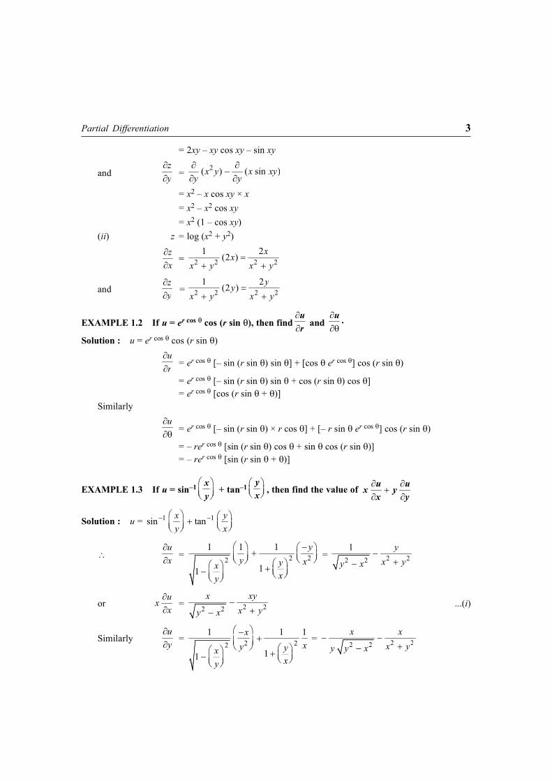
EXAMPLE 1.1 Evaluatezx and

zy , if

(i) z = x2y – x sin xy (ii) z = log (x2 + y2)Solution: (i) z = x2y – x sin xy

zx = 2xy – x x (sin xy) – sin xy × x (x)

= 2xy – x cos xy × y – sin xy × 1

Partial Differentiation 3

= 2xy – xy cos xy – sin xy

andzy = 2( ) ( sin )x y x xy

y y= x2 – x cos xy × x= x2 – x2 cos xy= x2 (1 – cos xy)

(ii) z = log (x2 + y2)

zx

= 2 2 2 21 2(2 ) xx

x y x y

andzy

= 2 2 2 21 2(2 ) yy

x y x y

EXAMPLE 1.2 If u = er cos cos (r sin ), then findur and

u·

Solution : u = er cos cos (r sin )ur = er cos [– sin (r sin ) sin ] + [cos er cos ] cos (r sin )

= er cos [– sin (r sin ) sin + cos (r sin ) cos ]= er cos [cos (r sin + )]

Similarlyu

= er cos [– sin (r sin ) × r cos ] + [– r sin er cos ] cos (r sin )

= – rer cos [sin (r sin ) cos + sin cos (r sin )]= – rer cos [sin (r sin + )]

EXAMPLE 1.3 If u = sin–1 xy

+ tan–1 yx , then find the value of u ux y

x y

Solution : u = 1 1sin tanx yy x

ux = 2 22

1 1 1

11

yy xyx

xy

= 2 22 2

1 yx yy x

oruxx

= 2 22 2

x xyx yy x

...(i)

Similarlyuy

= 2 22

1 1 1

11

xxy yx

xy

= 2 22 2

x xx yy y x

4 Engineering Mathematics

oruyy

= 2 22 2

x xyx yy x

...(ii)

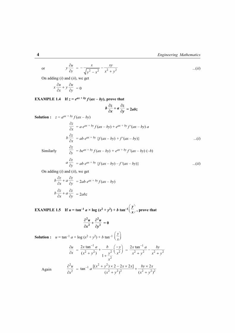
On adding (i) and (ii), we getu ux yx y = 0

EXAMPLE 1.4 If z = eax + by f (ax – by), prove thatz zb ax y = 2abz

Solution : z = aax + by f (ax – by)zx = a eax + by f (ax – by) + eax + by f (ax – by) a

zbx = ab eax + by {f (ax – by) + f (ax – by)} ...(i)

Similarlyzy = beax + by f (ax – by) + eax + by f (ax – by) (–b)

zay = ab eax + by {f (ax – by) – f (ax – by)} ...(ii)

On adding (i) and (ii), we getz zb ax y = 2ab eax + by f (ax – by)

z zb ax y = 2abz

EXAMPLE 1.5 If u = tan–1 a × log (x2 + y2) + b tan–1yx , prove that

u ux y

2 2

2 2 = 0

Solution : u = tan–1 a × log (x2 + y2) + b tan–1yx

ux =

1

2 2 2 2

2

2 tan( ) 1

x a b yx y y x

x

= 1

2 2 2 22 tanx a by

x y x y

Again2

2u

x=

2 21

2 2 2 2 2 2[( ) 2 2 2 ] 2tan

( ) ( )x y x x by xa

x y x y

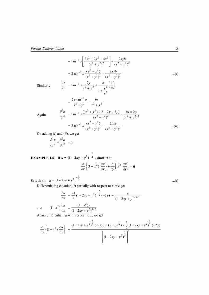
Partial Differentiation 5

=2 2 2

12 2 2 2 2 2

2 2 4 2tan( ) ( )

x y x xybax y x y

=2 2

12 2 2 2 2 2

( ) 22 tan

( ) ( )y x xyba

x y x y...(i)

Similarlyuy = 1

2 2 2

2

2 1tan1

y baxx y y

x

=1

2 2 2 22 tany a bx

x y x y

Again2

2u

y =2 2

12 2 2 2 2 2

[( ) 2 2 2 ] 2tan( ) ( )

x y y y bx yax y x y

=2 2

12 2 2 2 2 2

( ) 22 tan( ) ( )

x y bxyax y x y

...(ii)

On adding (i) and (ii), we get2 2

2 2x u

x y = 0

EXAMPLE 1.6 If u = xy y1

2 2(1 2 ) , show that

u ux yx x y y

2 2(1 ) = 0

Solution : u = 1

2 2(1 2 )xy y ...(i)Differentiating equation (i) partially with respect to x, we get

ux =

32 21 (1 2 ) ( 2 )

2xy y y = 2 3 / 2(1 2 )

yxy y

and 2(1 ) uxx =

2

2 3/ 2(1 )

(1 2 )x y

xy yAgain differentiating with respect to x, we get

2(1 )ux

x x =

3 12 2 22 2

232 2

3(1 2 ) ( 2 ) ( ) (1 2 ) ( 2 )2

(1 2 )

xy y xy y yx xy y y

xy y

6 Engineering Mathematics

=

12 2 2 2 22

2 3

(1 2 ) (1 2 ) ( 2 ) 3( )

(1 2 )

xy y xy y xy y x y

xy y

=2 2 3 2

2 5 / 22 2 3

(1 2 )x y xy xy y

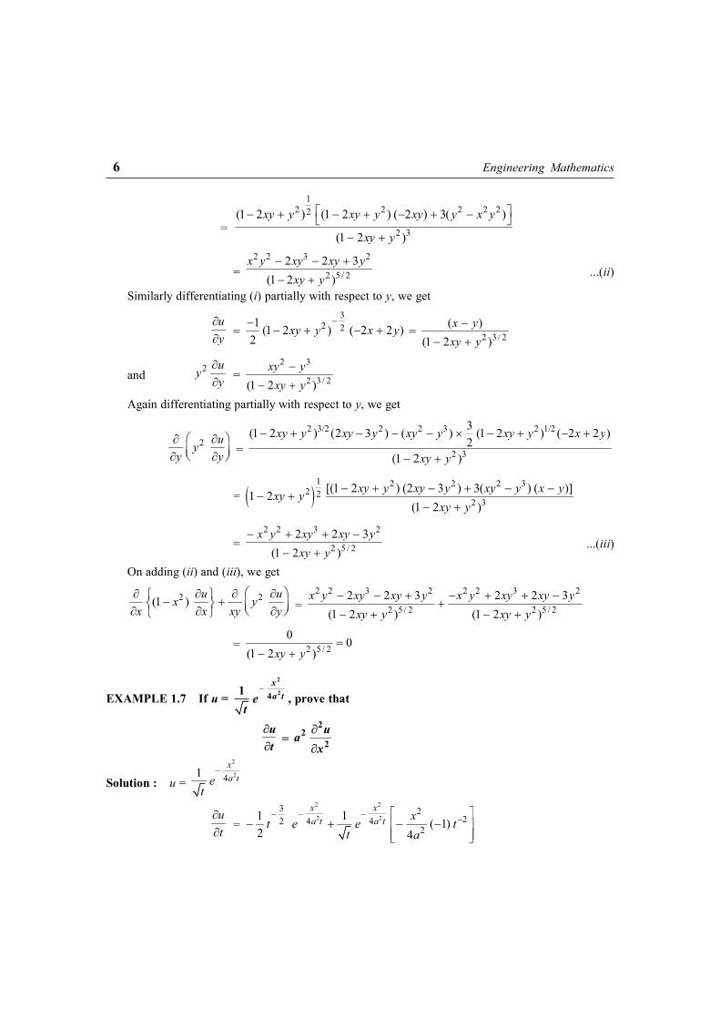
xy y ...(ii)

Similarly differentiating (i) partially with respect to y, we get

uy =

32 21 (1 2 ) ( 2 2 )

2xy y x y = 2 3 / 2

( )(1 2 )

x yxy y

and 2 uyy =

2 3

2 3 / 2(1 2 )xy y

xy yAgain differentiating partially with respect to y, we get

2 uyy y =

2 3/2 2 2 3 2 1/2

2 3

3(1 2 ) (2 3 ) ( ) (1 2 ) ( 2 2 )2

(1 2 )

xy y xy y xy y xy y x y

xy y

=1 2 2 2 3

2 22 3

[(1 2 ) (2 3 ) 3( ) ( )]1 2(1 2 )

xy y xy y xy y x yxy yxy y

=2 2 3 2

2 5 / 22 2 3

(1 2 )x y xy xy y

xy y...(iii)

On adding (ii) and (iii), we get

2 2(1 ) u ux yx x xy y =

2 2 3 2 2 2 3 2

2 5 / 2 2 5 / 22 2 3 2 2 3

(1 2 ) (1 2 )x y xy xy y x y xy xy y

xy y xy y

= 2 5 / 20 0

(1 2 )xy y

EXAMPLE 1.7 If u = xa te

t

2

241 , prove that

ut =

uax

22

2

Solution : u =

2

241xa te

t

ut =

2 2

2 23 2

24 422

1 1 ( 1)2 4

x xa t a t xt e e t

t a

A Textbook of Engineering Mathematics-I

Publisher : Manav RachnaPublishing House Pvt Ltd

Author : R S Goel and Y KSharma

Type the URL : http://www.kopykitab.com/product/1470

Get this eBook