Embed Size (px)
Citation preview

An Agent-based Model for Financial Vulnerability
Rick Bookstaber Office of Financial Research [email protected] Mark Paddrik Office of Financial Research [email protected] Brian Tivnan MITRE Corporation [email protected]
The Office of Financial Research (OFR) Working Paper Series allows members of the OFR staff
and their coauthors to disseminate preliminary research findings in a format intended to generate
discussion and critical comments. Papers in the OFR Working Paper Series are works in progress
and subject to revision.
Views and opinions expressed are those of the authors and do not necessarily represent official
positions or policy of the OFR, Treasury, or MITRE. Comments and suggestions for improvements
are welcome and should be directed to the authors. OFR Working Papers may be quoted without
additional permission.
14-05 | July 29, 2014Revised Sept. 2014

1
An Agent-based Model for Financial Vulnerability
Rick Bookstaber1
Mark Paddrik2
Brian Tivnan3
September 10, 2014
Brian Tivnan contributed by directing a team from MITRE to support many aspects of the paper. We wish to thank the members of that team: Zoe Henscheid and David Slater on visualizations and results analysis, Matt Koehler and Tony Bigbee on programming, and Matt McMahon and Christine Harvey on the design of experiments and related simulations. We also would like to thank Nathan Palmer for his work on the agent-based modeling, as well as Charlie Brummitt, Paul Glasserman, Benjamin Kay, Blake LeBaron, and Eric Schaanning for their valuable comments.
Views and opinions expressed are those of the authors and do not necessarily represent official positions or policy of the OFR, the U.S. Department of the Treasury, or MITRE. Comments are welcome, as are suggestions for improvements, and should be directed to the authors.
1 Office of Financial Research 2 Office of Financial Research 3 MITRE Corporation

2
Abstract
This paper describes an agent-based model for analyzing the vulnerability of the financial system to asset- and funding-based fire sales. The model views the dynamic interactions of agents in the financial system extending from the suppliers of funding through the intermediation and transformation functions of the bank/dealer to the financial institutions that use the funds to trade in the asset markets, and that pass collateral in the opposite direction. The model focuses on the intermediation functions of the bank/dealers in order to trace the path of shocks that come from sudden price declines, as well as shocks that come from the various agents, namely funding restrictions imposed by the cash providers, erosion of the credit of the bank/dealers, and investor redemptions by the buy-side financial institutions. The model demonstrates that it is the reaction to initial losses rather than the losses themselves that determine the extent of a crisis. By building on a detailed mapping of the transformations and dynamics of the financial system, the agent-based model provides an avenue toward risk management that can illuminate the pathways for the propagation of key crisis dynamics such as fire sales and funding runs.

3
1. Introduction We have a critical and unmet need to develop risk management methods that deal with the structure and dynamics of the financial system during financial crises. Risk management methods, most notably Value-at-Risk (VaR), are based on historical data and are simply not designed to work in a financial crisis. They cannot assess crisis events such as the progressive failure of the market for collateralized debt obligations, the successive failures of Bear Stearns, Fannie Mae, Freddie Mac, and Lehman, the path of counterparty exposures laid bare by the near-bankruptcy of AIG, or the more recent exposure of European banks to the risk of sovereign default. This is because a crisis is not similar to the past; it is not just a bad draw from the day-to-day workings of the financial system, and it is not a repeat of previous crises. Rather, it comes from the unleashing of a new dynamic, where shocks to markets and funding lead to a cycle of forced selling and to a reduction in liquidity that both magnifies the initial shocks and spreads the crisis to other markets and institutions. Each crisis is different, emanating from different shocks, affecting institutions that have different exposures to markets and to funding, often with financial instruments and sources of funding that did not even exist the last time around. There are a host of other measures that have come along to shore up the evident weaknesses of VaR, but by and large these all share the same core weakness: they depend on history, and are useful only insofar as the future looks like the past.4 We can think of these measures as “Risk Management Version 1.0.”
Recognizing the limitations of VaR-related risk measures, we have moved to “Risk Management Version 2.0” — stress testing. Stress testing can be used to pose scenarios, often encompassing movements in a wide variety of markets, that have not occurred in the past. Stress testing has become the focus of risk assessment in regulatory channels. However, it does not have a sterling record when it comes to large-scale financial crises.5 After the 2008 crisis, stress tests were buttressed by adding more severe scenarios and using more detailed data. Although stress tests take a step in the right direction by untethering the assessment of future crises from a rear view mirror view of historical data, they still fail in a critical respect. Stress testing does not incorporate the dynamics, feedback, and related complexities faced in a financial crisis.
For this, we require a “Version 3.0” of risk management, one that takes stress testing beyond the first-round effects of a shock to the individual financial institutions to ask: After the various institutions face the stress-induced losses, then what? How does that in turn alter the behavior of the banks and other market participants? How does the stress event play out and then affect other parts of the financial system? Answering these questions requires a rethinking of the models in
4 Bisias et al. (2012) enumerate risk measures based on analyzing historical risk. Battiston et al. (2012) and Greenwood et al. (2012) present models and related metrics designed to deal with the risk of a crisis, focusing on historical leverage levels. 5 For example, stress testing has been used since 2001 as a key component of the International Monetary Fund’s (IMF) Financial Sector Assessment Programs, but the IMF did not detect the structural weaknesses building up pre-crisis. One widely cited example is that of Iceland in International Monetary Fund (2008), critiqued by Alfaro and Drehmann (2009).

4
order to encompass the internal workings of the financial system, such as crowded trades, asymmetric information, liquidity shortages, and interconnectedness.
Discovering vulnerability to crisis requires a specification of system dynamics and behavior. Even if we are willing to make the leap of asserting that any one financial institution is not large enough for a stress to affect other parts of the financial system, if banks share similar exposures and thus are affected similarly by the stress, the aggregate effect will not be likely to reside in a ceteris paribus world. Furthermore, in the highly interrelated financial system, the aggregate effect will feed into yet other institutions and create adverse feedback and contagion.
Risks can build within the financial system as declines in prices and funding lead to forced liquidations in the face of reduced liquidity, which may create further pressure and cause a cascade and contagion among financial entities. For example, during booms, easy leverage and liquidity can breed market excesses. When market confidence turns, prices can rapidly readjust, leading to runs that put pressure on key funding sources for financial institutions. The drop in confidence also can lead to margin calls that force market participants to sell assets as a set of similarly challenged market participants rush to sell at the same time, which creates further pressure on market prices. The paths for this dynamic are generally characterized as asset-based and funding-based fire sales.6
Asset-based fire sales focus on the interaction between institutional investors, particularly leveraged investment firms such as hedge funds; their funding sources, notably the bank/dealer’s prime broker; and the asset markets where the forced sales occur. The fire sale occurs when there is a disruption to the system that forces a fund to sell positions. This disruption can occur through various channels: a price drop and resulting drop in asset value, a drop in funding or an increase in the margin rate from the prime broker, or a flow of investor redemptions. In any of these events, the fund reduces its assets, causing asset prices to drop, leading to further rounds of forced selling.
Funding-based fire sales focus on the interaction of the bank/dealer with its cash providers. It is triggered by a disruption in funding flows as might happen if there is a decline in the value of collateral or an erosion of confidence. This reduces the funding available to the trading desk, and its reduction in inventory again leads to a further price drop, so a funding-based and an asset-based fire sale can feed on one another. For example, the drop in collateral value can affect the finance desk directly. And a funding-based fire sale might precipitate an asset-based fire sale (the funding restrictions for the bank/dealer can reduce the funding available to the hedge fund through the prime broker, leading to asset liquidations) and vice versa.
To understand these critical aspects of the financial system, we need to be able to trace the path a shock follows as it propagates through the financial system, which requires us to understand the conduits for the transmission of information and financial flows and the rules employed by the 6 Models of these dynamics are discussed variously as fire sales, funding runs, liquidity spirals, leverage cycles, and panics (Shleifer and Vishny, 2011, Brunnermeier and Pedersen, 2009), leverage cycles (Adrian and Shin, 2013, Fostel and Geanakoplos, 2008), and panics (Gorton, 2010).

5
various financial entities based on their observations of the changing financial environment. Complicating this is the fact that the nature of the feedback tends to be scale-dependent. For example, a small change in price, funding, or a bank’s financial condition might be absorbed, but a large shock might trigger a destabilizing cascade. Currently, stress tests implicitly assume that banks are atomistic with respect to the financial markets; there is no mechanism to deal with the fact that banks are large enough for the effect of shocks on their balance sheet to then pass through to affect other market entities. A static representation may be adequate for some tasks, such as piercing balance-sheet opacity, but others, such as understanding the propagation of shocks through the financial system, require a dynamic approach.
Agent-based models are well suited to deal with the issues of crisis dynamics and feedback. Agent-based models follow the dynamics of agents, assessing their reaction to events period-by-period, and updating the system variables accordingly. An agent-based model incorporates heterogeneity and allows for the agents to use idiosyncratic and perhaps less-than-optimal rules for how financial institutions operate. The potential for agent-based models in this application is suggested by their application in other fields, such as tracing contagion in epidemiology, assessing points of congestion in traffic flows, and modeling crowd behavior and panics in building evacuations and in crowd stampedes.7
This paper develops the structure for an agent-based model to provide a system-wide view of the transformations and dynamic interactions of agents in the financial system extending from the suppliers of funding such as money market funds through the channels of the bank/dealer to the financial institutions that use the funds, as well as the collateral that passes in the opposite direction. In doing so, the paper provides an avenue toward risk management Version 3.0.8 The model focuses on the intermediation function of bank/dealers, such as their role in maturity, liquidity, credit, and collateral transformation. The paper also provides the mechanism to induce and trace the path of shocks that come from sudden price declines and from the various agents, namely funding restrictions imposed by the cash providers, erosion of credit of the bank/dealer, and investor redemptions by the buy-side financial institutions.
Model development is an engineering exercise in the sense that it is taking the characteristics of the market and established modeling tools to develop a practical assessment mechanism for vulnerabilities and supporting policy decision making. That is, with the underlying data and calibration in place, the model is intended to be applied as a risk tool.
7 The use of agent-based modeling for assessing financial vulnerabilities is discussed in Bookstaber (2012). A discussion of the value of agent-based modeling in juxtaposition to standard equilibrium economic models is presented in Farmer and Geanakoplos (2009), and a proposal for a program to apply agent-based modeling to the broad-scale task of financial and economic analysis is presented in Farmer et al. (2012). 8 The discussion of VaR, stress testing, and agent-based models as versions 1.0, 2.0, and 3.0 of risk management is introduced in Bookstaber et al. (2013).

6
2. Background
The Financial System
To evaluate the possible effects of fire-sale events, we need to consider the entire landscape of participants and the different roles they play in the financial system. Figure 1 is a schematic of this system showing the components of the bank/dealer, and its links to borrowers and to lenders.9 Figure 1 provides a view of the business activities performed by financial market participants with a directional display of the exchange of cash or securities.10 In the case of secured funding, the pathways are two-way streets; when there is funding in one direction, there is a flow of collateral in the other.
Figure 1: Financial System Funding Flows
Figure 1 is a diagram of the plumbing of critical components of the financial system. As funding, collateral and securities flow through the system, they are not simply shuffled from one institution to another. The institutions take the flows and transform them in various ways. The flows going from depositors to the long-term borrowers are subject to a maturity transformation, the standard banking function of taking in short term deposits and making longer-maturity loans.
9 This figure and related discussion is adapted from Aguiar et al. (2014). 10 Montagna and Kok (2013) present a network model that reflects several of these channels through which bank/dealers interact, namely lending, market-making and liquidity provisioning, and common portfolio exposures.

7
The flows of funding from the cash providers through secured funding and prime brokers to hedge funds are subject to a credit transformation; the less creditworthy hedge funds receive funding from lenders who demand very high credit risk. The flows between the financial institutions on either side of the bank/dealer’s trading desk are subject to a liquidity transformation, where less liquid assets, such as mortgages, are structured into debt instruments with liquid tranches, and where market making provides liquidity. And the participants in the derivatives area are subject to risk transformations, where the return distribution of assets is changed, such as by issuing options.
We are interested in understanding the function of the various components play in producing shocks and their role, given a shock, in the subsequent dynamics as the effects of the shock propagate through this system. To do so we need to know not only how the agents are connected, but also what transformations are occurring. This can be served by the agent-based modeling approach. The rest of this section will walk through the various parts of this diagram and explain the basic functions they perform in an agent-based context. As Figure 1 suggests, we are focused only on a microcosm of the broader financial system, one centered on the flow of funding and securities that are central to asset- and funding-based fire sales. We thus leave much of the landscape — depositors, structured products, corporate loans — unexplored.
Lenders: The Cash Provider
The cash providers include asset managers, pension funds, insurance companies, and security lenders, but most centrally, money market funds. Money market funds are not a source of durable funding because under regulation 2a-7 they are limited to provide only short-term secured funding. Also, during a stress event, money market fund investors may redeem their shares, requiring the money market fund to liquidate its investments.
Bank/Dealers
The bank/dealer acts as an intermediary between buyers and sellers of securities, and between lenders and borrowers of funding. Figure 1 separates the functional units and the related flows, allowing us to better distinguish the transformations they present. Each of the following desks acts as an agent in either perform this transformation or as a self-governing mechanism to insure the bank/dealer is secure of the risks it takes on.
Prime Broker
The prime broker provides financial services to hedge funds, including leverage through margin loans and securities for short activity. A hedge fund looking for securities to cover their short will provide cash to the prime broker to source these securities. The prime broker is an intermediary between two functions of the hedge fund, its need for financing to lever its long positions, and its need for borrowing securities for its short positions (and in the process providing cash to the prime broker). A hedge fund looking for leverage provides securities to the

8
prime broker in order to borrow cash on margin. The bank/dealer can finance margin loans by hypothecating these securities.
Finance Desk
The bank/dealer's financing operations include secured funding, where the financing desk borrows cash with securities used as collateral. Secured financing is used to fund securities owned by the bank/dealer as well as rehypothecatable securities received as collateral from clients. The financing desk also takes an intermediary role in providing clients financing by reversing in collateral from clients and sourcing funding through the repo market. These client financing transactions are typically referred to as “matched book.” Through this function, the bank/dealer uses its access to secured funding to provide leverage to clients primarily for fixed income products, filling the role the prime broker does for equities.
Trading Desk
The bank/dealer manages inventory in its market making activities, the bulk of which is financed through secured funding. The trading desk’s inventories includes long exposure from clients selling securities, and short positions to facilitate client purchases. Shorts are covered by borrowing securities from securities lenders or through the central counterparties (such as other dealers). Though not treated in this model, trading activity also includes the repackaging of inventory as securitized products.
Derivatives Desk
The bank/dealer executes derivative transactions for itself and for clients, with the primary motivation being to hedge or reduce risk in the underlying position. Derivatives include products such as futures, forwards, swaps, and options. Derivatives can be cleared through exchanges or executed bilaterally, and bilateral derivative trades can be collateralized or uncollateralized. We will focus on counterparty risk in the derivatives desk, and any market risk will be subsumed by the trading desk.
Treasury
The bank/dealer’s treasury function raises longer term unsecured financing for the firm through equity and debt issuances, which can include short term debt, such as commercial paper. The equity provides the capital base for all funding operations, and the equity and unsecured debt is used to fund assets which are difficult to fund by secured funding sources.
Intermediaries
Figure 1 also depicts key funding intermediaries such as triparty agents, central counterparties, and clearing exchanges. These are important potential means for the transmission of shocks, but will not be treated in the current model.

9
Borrowers: Hedge Funds
Hedge funds use the prime broker to obtain financing for leveraged long positions and to borrow securities for short positions. For the former they provide collateral, and for the latter they provide cash. The hedge funds represent the far broader universe of asset managers and other institutional investors, but unlike many others in that space, hedge funds can take on leverage, a critical component of asset-based fire sales. A standard asset manager can be introduced into the model as a hedge fund that cannot short and cannot employ leverage.
3. Objectives
Before getting into the details of the model, which we will do in Section 4, we will illustrate the objectives of the model by showing how the model can trace a shock as it reverberates through the system. Although the model can be applied to a system with many agents, here we will apply the model for a tractable network of three assets, two hedge funds, two bank/dealers, and a single cash provider that treats each bank/dealer separately. Figure 2 gives a general description of how the various agents in the model relate. In this figure, the Bank/Dealer 1 (BD1) and Hedge Fund 1 (HF1) hold equal weights in Asset 1 (A1) and Asset 2 (A2), and Bank/Dealer 2 (BD2) and Hedge Fund 2 (HF2) hold equal weights in Asset 2 (A2) and Asset 3 (A3). The Cash Provider (CP1) supplies funding to the bank/dealers, which in turn supply funding to the hedge funds.
Figure 2: Diagram of Simulated Financial System Network of 3x2x2x1 Model
Even in this simple specification of the model, the interactions of the agents and how those interactions are affected by changes in the parameters remain complex.
Model Dynamics and the Propagation of Shocks
There has been a surge in network-related research of the financial system in response to the role of interconnections in the 2008 crisis. The networks depicted for the financial system are often impressive in terms of their complexity, with dozens of nodes representing the various

10
institutional entities, and often hundreds of links between the nodes.11 Although the network depictions can give a startling visualization of the magnitude of interrelationships, to date they have not provided much insight into the risks arising from the complexity and the interrelationships. A difficulty facing the network approach is that in isolation a network representation does not depict how the nodes transform the flows, nor how the flows carry risk from one node to another. Figure 2 illustrates the point that the edges between agents can tie to any of several functional units; for example, a bank/dealer might link to another bank/dealer as a derivative counterparty or as a security lender. In the first case, they would be subject to credit shocks, while in the second, they would be subject to funding shocks. Applying a network approach requires revealing the processes within the institutions that produce the various financial transformations and then delivering the transformed flows to other institutions. Absent this, it gives a snap shot at a particular time rather than tracking the dynamics of the process.
11 Network research has spanned areas including systemic failures due to contagion of counterparty risk and credit relationship (Acemoglu et al., 2013) and the related central counterparty clearing networks (Song et al., 2014); networks of exposures of banks through the interbank and repo markets (Allen, and Babus, 2009); and of the distribution of liquidity throughout the financial system through the federal funds market (Bech et al., 2008), ]. In addition, network analysis is being applied to understand the financial systems within specific countries. For example, research on the network for interbank market and overnight funding and its implications for the contagion of financial shocks and liquidity has been analyzed for the financial systems of Belgium (Degryse, et al., 2007), England (Becher et al. 2008), Italy (Iori et al. 2008), Germany (Upper and Worms, 2004), and Brazil (Cont et al., 2012).
11
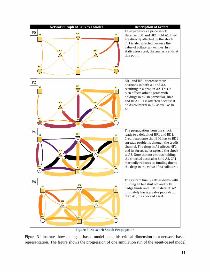
Network Graph of 3x2x2x1 Model Description of Events
A1 experiences a price shock. Because BD1 and HF1 hold A1, they are directly affected by the shock. CP1 is also affected because the value of collateral declines. In a static stress test, the analysis ends at this point.
BD1 and HF1 decrease their positions in both A1 and A2, resulting in a drop in A2. This in turn affects other agents with holdings in A2, in particular, BD2 and HF2. CP1 is affected because it holds collateral in A2 as well as in A1.
The propagation from the shock leads to a default of HF1 and BD1. Credit exposure that BD2 has to BD1 spreads problems through the credit channel. The drop in A2 affects HF2, and its forced sales spread the shock to A3. Note that no entities holding the shocked asset also hold A3. CP1 markedly reduces its funding due to the drop in the value of its collateral.
The system finally settles down with funding all but shut off, and both hedge funds and BD1 in default. A2 ultimately has a greater price drop than A1, the shocked asset.
Figure 3: Network Shock Propagation
Figure 3 illustrates how the agent-based model adds this critical dimension to a network-based representation. The figure shows the progression of one simulation run of the agent-based model
P2
P0
P4
P6

12
for the parameter set we are employing in this section. Each period in the progression is depicted by a network showing which agents (nodes) influence other agents. The networks are depicted as an output of the model, and the network structure changes period-by-period as the environment changes due to the agents' actions and as the agents adapt accordingly.
In this figure, the dark outline for the nodes shows the agents’ initial size (in this case we assume all of the agents have the same starting capital and all initial prices are identical), and the shrinking of the colored area within the node is proportional to the decline in capital in the case of the hedge funds and bank/dealers, the reduction in funding in the case of the cash provider, and the drop in prices in the case of the assets. If the color within the node disappears, then that agent has defaulted.
Each edge in the network denotes the relational impact of one node, 𝑖, on another, 𝑗, based on the relationship that exists in the agent-based model, normalized by running the simulation a number of times with variations on each variable. As described in equations (1) and (2), the width of the edge shows the cumulative effect of the transmission with respect to 𝑡 periods and the 𝑛 runs of the simulation, and the color of the edge in the figure shows the intensity of the interaction in the current period — a darker color means greater intensity or change in the system relative to other runs and periods observed.
∑ �𝐸𝐸𝐸𝐸𝑡𝑖𝑖�𝑇
1
max𝑛
∑ �𝐸𝐸𝐸𝐸𝑡𝑖𝑖�𝑇
1 (1)
∑ �𝐸𝐸𝐸𝐸𝑡𝑖𝑗�𝑇
1 − min𝑛∑ �𝐸𝐸𝐸𝐸𝑡
𝑖𝑗�𝑇1
�max𝑛∑ �𝐸𝐸𝐸𝐸𝑡
𝑖𝑗�𝑇1 − min
𝑛∑ �𝐸𝐸𝐸𝐸𝑡
𝑖𝑗�𝑇1 �
(2)
Cumulative Edge Width Intensity of Interaction
For this example the shock does not have far to go before it embroils the system; it reverberates through the system and runs its course in six periods. Although not shown here, we could present a network dynamic that combines these shocks to occur in sequence. For example, in addition to the asset shock, we could insert an exogenous funding or credit shock in one of the periods. In such cases the progress of the dynamic will generally be extended.
Sources of Shocks to the Financial System: Prices, Funding, Credit, and Redemption Shocks
The propagation analysis of liquidity, leverage, and allocations presented are based on a price shock as the triggering event. The model also allows for shocks based on a reduction in funding by the cash provider, a drop in credit worthiness of the bank/dealers, and a redemption shock to the hedge funds. Figure 4 illustrates each of these sources of an initial shock in the network diagram, demonstrating how they have notably different origins.

13
Price Shock Funding Shock
Credit Shock Redemption Shock
Figure 4: Network View of Initial Shock Propogation
We can look at the spread of the shock from each of these sources as the triggering event propagates, illustrated in Figure 5, which shows sequential heat maps for the timing of events after the initial shock. Rather than looking at the effects on capital and prices as we have in the previous results, here we look at the actions of the agents, specifically at their forced liquidations. Figure 5 shows the propagation of the shock, but rather than tracing its path during one simulation run, here we show the results over many simulations. The heat maps have the initial shock in period 0, and then are shaded according to the frequency of the various events in the subsequent periods.
The severity and extent of the propagation depends on the parameters used in the simulation, such as the leverage and allocations of the agents, and liquidity of the markets. However, the shocks themselves can have unique impact paths to the firms in the system such that we can see events in parallel or series to one another depending on where it starts and how quickly a shock can makes its way through the system. Figure 5-A shows the price shock in A1 principally affects HF1, and extends out to affect the other agents only when the forced selling is severe enough to create contagion to A2. Similarly, Figure 5-B shows a redemption shock for HF1 moves out to first affect BD1, which shares both assets held by HF1, and then affecting HF2 and BD2. By contrast, the funding shock, a reduction in the funding provided by the cash provider, CP1, to both of the bank/dealers shown in Figure 5-C, rapidly affects all of the agents.

14
Figure 5: Heat Map of Shock Propogation over Multiple Periods
4. The Agent-based Model The objective of the agent-based model is to take the relationships and functions of the various participants important for the propagation of financial crises and do so in a way that can be populated with available data.
The model we have built focuses on three types of agents operating in an asset and a funding market: (a) The hedge fund (HF) that participates in asset markets and require funding; (b) the cash provider (CP) that acts as funding sources by pooling investors assets; (c) and the bank/dealer (BD) that has several subagents that allows the bank/dealer to participate in asset markets, provide funding to hedge funds and other bank dealers, and lastly require funding from the cash provider. These agents and the flows between them are discussed in Section 2. Here we add further detail in order to show how each agent functions within the model in making decisions.

15
Asset Market
Asset markets in this model are meant to represent any number of different markets, equities, futures, commodities, mortgage backed securities, etc. There is an extensive literature applying agent-based models to market microstructure.12 However, because the focus here is on periods of market dislocation, we will apply a simple assumption for the day-to-day movement of prices. In particular, for the purposes of the development of this model we assume that absent event-driven selling all markets, 𝑀, follow a standard mechanism in which assets are priced, 𝑃𝑚, from one period to the next based on a random movement depicted by 𝑃𝑅𝑚𝑅 , which is 𝑁(0,𝜎𝑚). In the case of event-driven selling, the total quantity sold in market m during period t is denoted by 𝐸𝐷𝑆 𝑚
𝑇𝑇𝑡𝑇𝑇(𝑡); this is the net quantity of shares of 𝑁 hedge funds, 𝐸𝐷𝑆𝑚,𝑛𝐻𝐹 , and of 𝐾 trading desks
from the bank/dealers, 𝐸𝐷𝑆𝑚,𝑘𝐵𝐷 , need to sell in response to an extraordinary event; and (c) the
price elasticity of demand, 𝐵𝑚.
𝐸𝐷𝑆𝑚𝑇𝑇𝑡𝑇𝑇(𝑡) = �𝐸𝐷𝑆𝑚,𝑖
𝐻𝐹(𝑡)𝑁
𝑖=1
+ �𝐸𝐷𝑆𝑚,𝑖𝐵𝐷(𝑡)
𝐾
𝑖=1
(3)
𝑃𝑅𝑚(𝑡) = 𝐵𝑚𝐸𝐷𝑆𝑚𝑇𝑇𝑡𝑇𝑇(𝑡) + 𝑃𝑅𝑚𝑅 (t) (4)
𝑃𝑚(𝑡 + 1) = max(0,𝑃𝑚(𝑡)�1 + 𝑃𝑅𝑚(𝑡)�) (5)
The agents are considered atomistic with respect to the market except during times of forced liquidation, and absent such forced sales the day-to-day movement in prices takes on a simple random process. That is, the firms are assumed to execute their buying and selling by placing orders, 𝑂𝑖(𝑡), which typically do not impact the price of assets. This is what would be expected during normal times, because the agents have the option of spacing out their trades to minimize the market impact. What does matter and is the focus of the model are the occasions where a shock leads a bank/dealer or hedge fund into fire sale mode; that is, where an agent is forced to liquidate without regard to market implications. In those cases, we assume that their executed orders can have a price impact, denoted by 𝐸𝐷𝑆𝑖
𝐻𝐹,𝐵𝐷(𝑡).
Note that using the product of 𝐵𝑚 and the quantity of forced sales will lead to a larger and larger impact from forced selling as prices drop, because for a lower price there will need to be higher
12 The development of agent-based models of financial markets is surveyed in LeBaron (2006). Agent-based market models address two issues identified in LeBaron (2001a): the representation of the agents and the representation of the trading mechanism. For the evolution of agents, models began in the early 1990s with the Santa Fe Institute Artificial Stock Market model. Following this model, Lux et al. (1999) and LeBaron (2001b) introduced models with market orders, and Ghoulmie et al. (2005) then developed a model with traders that have heterogeneous trading thresholds that adapt based upon performance feedback. Models focused on trading mechanisms began with Maslov (2000) and then were extended by Darley et al (2001) and Farmer et al (2005). The Farmer model, later extended by Preis et al. (2006), builds a model of zero-intelligence traders active within the structure of a continuous, double auction placing market and limit orders.

16
quantity sold to sell the same dollar amount. This means that we are assuming liquidity drops proportionately with price; that is, liquidity is based on the total market value or float available to sell. An alternative is to have forced selling be based on a dollar amount rather than a quantity. This, of course, will change the units and size of 𝐵𝑚,13 or we can add a further term to the determination of 𝐵𝑚 to allow it to increase as the fire sale evolves. For example, the beta can increase as a function of the forced selling that enters the market.14
Cash Provider
The cash provider, 𝑐, lends to the finance desk based on the dollar value of the collateral it receives and a haircut it sets for bank/dealer, 𝑘, 𝐻𝐶𝑐,𝑘. The haircut is based on the perceived creditworthiness of a borrower that will be used to cut the value of the asset used as collateral, 𝐶𝐴𝑘(t), a percent of its current market value. The target amount that will be lent based on the haircut, which can be modeled to vary based on the cash provider’s decision rule, is:
𝐿𝑐,𝑘𝑇𝑇𝑅𝑅𝑅𝑡(t) = 𝐶𝐴𝑘(t)�1 − 𝐻𝐶𝑐,𝑘(t)� (6)
The loan is checked to ensure it does not go over a maximum dollar amount the cash provider is willing to lend independent of any collateral or haircut, 𝐿𝑐,𝑘
𝑀𝑇𝑀:
𝐿𝑐,𝑘(t) = min�𝐿𝑐,𝑘𝑀𝑇𝑀(t), 𝐿𝑐,𝑘
𝑇𝑇𝑅𝑅𝑅𝑡(t)� (7)
This last part of its decision rule reflects the fact that many cash providers are extremely risk averse and have limits in their ability to hold and liquidate collateral, so they will not lend more than a given amount, no matter what the size and nature of the collateral. If 𝑳𝑨,𝒌
𝑴𝑨𝑴(𝐭) is hit the 𝑪𝑨𝒌(𝐭) is revised to reflect the amount of collateral it will submit.
Hedge Funds
Hedge funds represent the broader range of the institutional investment space. We focus on hedge funds because leverage is the critical feature that creates asset-based fire sales. The hedge fund uses its capital and cash borrowed from the prime broker of a bank/dealer to finance its buying of assets. The broader universe of asset managers can be considered as unleveraged hedge funds in this model. As a practical matter, many apparently unleveraged asset managers have leverage gained through secured lending transactions and derivative exposure. Also, other
13 Market impact may increase with ongoing forced selling for two reasons. First, investors may be slow to provide liquidity because they are inattentive to the demand for immediacy of those facing forced sales as noted in Duffie (2010), and beyond inattentiveness (which will become less of an issue as the market dynamics dominate the investment new cycle), liquidity supply will be slower to come than the liquidity demand because of heterogeneous decision cycles; many investors, particularly the long-term investors are not set up structurally to make quick decisions, as noted in the model of market dynamics in the face of heterogeneous decision cycles in Bookstaber et al. (2014). Second, if some traders are forced to liquidate, and this becomes known to other traders, market impact will increase due to predatory pricing, as noted by Brunnermeier and Pedersen (2005). Rather than increasing, liquidity supply may reduce as prices and indeed the price drop can be precipitated in part from the strategic selling. 14𝛣𝑚 = 𝛽𝑚 + 𝜆𝑚 ∗ ∑ 𝐸𝐷𝑆𝑚𝑇𝑇𝑡𝑇𝑇(𝑖𝑡−𝑛
𝑖=𝑡 ), where 𝛽𝑚is the baseline 𝛣𝑚value and 𝜆𝑚is the constant that is a multiple based on the sum of total 𝐸𝐷𝑆𝑚𝑇𝑇𝑡𝑇𝑇from period 𝑡 to 𝑡 – 𝑛 periods in the past.

17
parts of the institutional investor space face redemption risk, which we will include in the model, and which make them susceptible to forced sale dynamics similar to those that leverage creates for the hedge funds.
The hedge funds use three leverage constraints:
1. Leverage Maximum, 𝐿𝐸𝐿𝑛𝑀𝑇𝑀(𝑡) which is set by the prime broker of the bank/dealer, 𝑘, which the hedge fund is using for financing15.
𝐿𝐸𝐿𝑛𝑀𝑇𝑀(𝑡) =1
�𝐻𝐶𝑐,𝑘(t)� (8)
2. Leverage Buffer, 𝐿𝐸𝐿𝑛𝐵𝑢𝑓𝑓𝐸𝑟(𝑡), that is some percent of 𝐿𝐸𝐿𝑛𝑀𝑇𝑀(𝑡) which the hedge fund will try not to exceed.
𝐿𝐸𝐿𝑛𝐵𝐵𝐵𝐵𝑅𝑅(𝑡) = 𝐿𝐸𝐿𝑛𝑀𝐶𝑥(𝑡)𝐿𝐸𝐿𝑛𝐵𝑢𝑓𝑓𝐸𝑟 𝑅𝐶𝑡𝐸 (9)
3. Leverage Target, 𝐿𝐸𝐿𝑛𝑇𝑇𝑅𝑅𝑅𝑡(𝑡), a leverage target which is some percent of
𝐿𝐸𝐿𝑛𝐵𝑢𝑓𝑓𝐸𝑟(𝑡).16
𝐿𝐸𝐿𝑛𝑇𝑇𝑅𝑅𝑅𝑡(𝑡) = 𝐿𝐸𝐿𝑛
𝐵𝐵𝐵𝐵𝑅𝑅(𝑡)𝐿𝐸𝐿𝑛𝑇𝑇𝑅𝑅𝑅𝑡 𝑅𝑇𝑡𝑅 (10)
Both 𝐿𝐸𝐿𝑛𝐵𝐵𝐵𝐵𝑅𝑅𝑅𝑇𝑡𝑅and 𝐿𝐸𝐿𝑛
𝑇𝑇𝑅𝑅𝑅𝑡𝑅𝑇𝑡𝑅are variables set by the hedge fund to govern the percentage it wants to be away from 𝐿𝐸𝐿𝑛𝑀𝑇𝑀(𝑡).17 Additionally, the hedge fund has two other parameters, an initial capital, 𝐶𝐶𝐶𝑛(0), which it uses to fund all of its initial activities; and an asset allocation vector, 𝐴𝑛𝐴𝑇𝑇𝑇𝑐𝑇𝑡𝑖𝑇𝑛, which is used to determine how it should allocate its capital between the 𝑀 assets.18
15 In this specification, the 𝐻𝐶𝑐,𝑘(t) is simply the inverse of the 𝐿𝐸𝐿𝑛𝑀𝑇𝑀(𝑡). 16 Note that 𝐿𝐸𝐿𝑛𝑀𝑇𝑀(𝑡) ≥ 𝐿𝐸𝐿𝑛
𝐵𝐵𝐵𝐵𝑅𝑅(𝑡) ≥ 𝐿𝐸𝐿𝑛𝑇𝑇𝑅𝑅𝑅𝑡(𝑡)
17 A theme in the academic literature is that there is an inverse relationship between the level of risk in the market — usually represented as the volatility of asset prices or the Value-at-Risk for institutions — and the amount of leverage taken. The mechanism for this is readily apparent; should bank/dealers seek to maintain a constant value for VaR/equity, as suggested by Adrian and Shin (2013), then if volatility is two-thirds its previous level, why not lever one and a half times as much? Brunnermeier and Sannikov (2012) discuss the interactions of low volatility, leverage, and low risk premium. The model can readily make leverage adjustments based on VaR, but we do not have the reduction of leverage in the face of increased risk in the post-shock period come through the VaR/equity mechanism because over the short time period of the types of crises we are considering the conventional computation of VaR, which uses six months-to-two years of history, will not have a demonstrable change. Rather, the post-shock relationship between risk and leverage exists in our model through the funding channel. In particular, the cash provider changes its funding based on the liquidity ratio of the bank/dealer, which it monitors on a daily basis during periods of crisis, as well as on the value of its collateral. A drop in the liquidity ratio will increase the risk of the bank/dealer, leading to a drop in leverage. 18 The asset allocation is held constant throughout the model.

18
For every period t, the hedge fund has the following set of variables and actions it must maintain in order to appropriately manage its asset portfolio. Its goal for every period is to determine the appropriate amount of shares of asset m, 𝑄𝑛,𝑚.19
i. It determines the current value of assets, 𝐴𝑛(𝑡), it has under management
𝐴𝑛(𝑡) = �𝑄𝑛,𝑖(𝑡 − 1)𝑃𝑖(𝑡 − 1)
𝑀
𝑖=1
(11)
so that it can appropriately distribute its capital based on the dollar assets held at the start of period t, using prices from the previous period because prices are determined at the end of the period.20
ii. The hedge fund receives a haircut, 𝐻𝐶𝑐,𝑘, from the prime broker, and computes its leverage value of 𝐿𝐸𝐿𝑛𝑀𝑇𝑀(𝑡), 𝐿𝐸𝐿𝑛
𝐵𝐵𝐵𝐵𝑅𝑅(𝑡), and 𝐿𝐸𝐿𝑛𝑇𝑇𝑅𝑅𝑅𝑡(𝑡).
iii. The hedge fund evaluates the trading price profit or loss, 𝑃𝐿𝑛, it had due to selling or buying assets at the end of previous period, 𝑡 − 1, this accounts for the previous periods trades price due to the models daily sequence of actions.
𝑃𝐿𝑛(𝑡) = ��𝑂𝑛,𝑖(𝑡) + 𝐸𝐷𝑆𝑛,𝑖
𝐻𝐹�(𝑃𝑖(𝑡 − 1) − 𝑃𝑖(𝑡 − 2))𝑀
𝑖=1
(12)
iv. The hedge fund computes the value of its capital, where 𝐹𝑛𝐻𝐹(𝑡 − 1) is the cash borrowed from the finance desk at the end of period t-1. This is the funding that is available for period t decision-making.
𝐶𝐶𝐶𝑛(𝑡) = 𝐴𝑛(𝑡) − 𝐹𝑛𝐻𝐹(𝑡 − 1) − 𝑃𝐿𝑛(𝑡) (13)
v. The hedge fund can now determine how well it has been able to both meet the constraint and target leverage by calculating the current leverage it has after the previous price movements.
𝐿𝐸𝐿𝑛𝐶𝐵𝑅𝑅𝑅𝑛𝑡(𝑡) = 𝐴𝑛(𝑡) /𝐶𝐶𝐶𝑛(𝑡) (14)
vi. Given its new capital level, the hedge fund computes its target asset level; the dollar assets that the hedge fund would own at its target leverage.
𝐴𝑛𝑇𝑇𝑅𝑅𝑅𝑡(t) = 𝐶𝐶𝐶𝑛(𝑡)𝐿𝐸𝐿𝑛
𝑇𝑇𝑅𝑅𝑅𝑡(𝑡) (15)
19 Where 𝑄𝑚(𝑡) ≥ 0, since we do not considering short positions in this model. They can be readily added, but for crises of potential systemic importance it is drops in prices, not increases that are the issue. Short positions also can be important sources of financing, but that will be subsumed in the general cash provider. 20 The hedge fund essentially enters market orders. Since we are concerned with large funds here, this is a reasonable representation of the execution of their trading programs, especially during times of stress, where time matters more than price.

19
vii. This assessment of total amount of assets it wants to have under management and the change in prices over the previous period it will use this to determine whether it will need to buy or sell each asset.
a. If 𝐿𝐸𝐿𝑛𝐶𝐵𝑅𝑅𝑅𝑛𝑡(𝑡) ≥ 𝐿𝐸𝐿𝑛𝑀𝑇𝑀(𝑡), the hedge fund receives a forced margin call and therefore must reduce its assets, liquidating enough shares, that is generating a 𝐸𝐷𝑆𝑛𝐻𝐹 , to get back to the 𝐿𝐸𝐿𝑛
𝐵𝐵𝐵𝐵𝑅𝑅(𝑡). Stated another way, the difference between 𝐿𝐸𝐿𝑛𝑀𝑇𝑀(𝑡) and 𝐿𝐸𝐿𝑛
𝐵𝐵𝐵𝐵𝑅𝑅(𝑡) can be considered the maintenance margin. Therefore, 𝐸𝐷𝑆𝑛𝐻𝐹(𝑡), the number of shares that will be sold is:
𝐸𝐷𝑆𝑛𝐻𝐹(𝑡) = �min�0,
−�𝐴𝑛,𝑖(𝑡) − 𝐿𝐸𝐿𝑛𝐵𝐵𝐵𝐵𝑅𝑅(𝑡)𝐶𝐶𝐶𝑛(𝑡)� 𝐴𝑖𝐴𝑇𝑇𝑇𝑐𝑇𝑡𝑖𝑇𝑛(t)
𝑃𝑖(𝑡 − 1) �𝑀
𝑖=1
(16)
b. If 𝐿𝐸𝐿𝑛𝐶𝐵𝑅𝑅𝑅𝑛𝑡(𝑡) < 𝐿𝐸𝐿𝑛𝑀𝑇𝑀(𝑡), the hedge fund moves toward its target assets, 𝐴𝑛𝑇𝑇𝑅𝑅𝑅𝑡 dictated by its 𝐿𝐸𝐿𝑛
𝑇𝑇𝑅𝑅𝑅𝑡(𝑡). This tendency reflects its day-to-day position adjustments that do not impact price and so do not pass through to the pricing function. The number of shares, 𝑂𝑛,𝑚(𝑡), of asset m that will be bought or sold by the hedge fund n:
𝑂𝑛,𝑚(𝑡) =
�𝐴𝑛,𝑚𝑇𝑎𝑟𝑔𝑒𝑡(t)−𝐴𝑛,𝑚(𝑡)�
𝑃𝑚(𝑡−1) 𝐴𝑛,𝑚𝐴𝑇𝑇𝑇𝑐𝑇𝑡𝑖𝑇𝑛(𝑡) (17)
viii. This updates the quantity of share held by the hedge fund to 𝑄𝑛(𝑡) based on the trading decisions made as a result of 𝐸𝐷𝑆𝑛𝐻𝐹(𝑡) or 𝑂𝑛(𝑡).21 This then allows the hedge fund to determine how much funding, 𝐹𝑛𝐻𝐹(𝑡), it will need achieve 𝑄𝑛,𝑚(𝑡) based on its current capital.
𝑄𝑛,𝑚(𝑡) = 𝑄𝑛,𝑚(𝑡 − 1) + 𝑂𝑛,𝑚(𝑡) + 𝐸𝐷𝑆𝑛,𝑚𝐻𝐹 (𝑡) (18)
𝐹𝑛𝐻𝐹(𝑡) = 𝐴𝑛(𝑡) − 𝐶𝐶𝐶𝑛(𝑡) = �𝑄𝑛,𝑖(𝑡 − 1)𝑃𝑖(𝑡 − 1)
𝑀
𝑖=1
− 𝐶𝐶𝐶𝑛(𝑡) (19)
21 EDS < 0 and O_n(t) < 0 corresponds to selling, whereas O_n(t) > 0 corresponds to buying.

20
This completes the “day-in-the-life” sequential process that each hedge fund must go through in determining its portfolio management. If at the end of any period the hedge fund’s 𝑪𝑨𝑪𝒌 is ≤ 𝟎, it will suffer a default that will cause it to sell all it assets during the next period, 𝑨 + 𝟏, and will no longer allow it to participate within the financial system throughout the rest of the model’s run. Although for a given shock, it is unlikely that all hedge funds will become embroiled in a forced sale, and those that do will not always die.
Just as detailed for hedge fund here, the bank/dealer and indeed each of the other types of agents follow a “day-in-the-life” sequence of decisions based on their observations of the results from the previous period.
Bank/Dealer
The bank/dealer acts as an intermediary between buyers and sellers of securities and between lenders and borrowers of funding. As we previously outlined, it employs a number of subagents to do the various tasks. Just as the hedge fund can be modeled to represent a wider set of institutions, so the bank/dealer can be modeled to represent agents that only have a subset of these functions. For example, there might be an intermediary that only provides the market making function of the trading desk, or that does not have a derivatives function. Thus, the bank/dealer category encompasses more than the major bank/dealer institutions that provide all these functions.
Prime Broker
The prime broker acts as the agent that interacts with all the hedge funds that bank/dealer 𝑘 does business with (a subset 𝑁𝑘 of all 𝑁 hedge funds). The prime broker’s job is to gather the collateral of the hedge funds, 𝐶𝐴𝑘𝑃𝐵, so that it can then look for funding, 𝐹𝑘𝑃𝐵, from the cash providers for any loans that hedge funds need to cover their leveraged positions.
𝐶𝐴𝑘𝑃𝐵(𝑡) = �
𝐴𝑖(𝑡) − 𝐶𝐶𝐶𝑖(𝑡)�1 − 𝐻𝐶𝑐,𝑘(t)�
𝑁𝑘
𝑖=1
𝑓𝑜𝑟 i ∈ 𝑁𝑘 (20)
As stated earlier, we make the simplifying assumption that the prime broker passes the funding from the finance desk through with no further haircuts, so the collateral of the prime broker is equal to that of the sum of the hedge funds it services. Once the funding desk receives the capital from the cash provider it distributes it to the prime brokers, which then passes the funding to the hedge funds.
𝐹𝑘𝑃𝐵(𝑡) = �𝐹𝑖(𝑡)
𝑁𝑘
𝑖=1
= �𝐴𝑖(𝑡) − 𝐶𝐶𝐶𝑖(𝑡)𝑁𝑘
𝑖=1
𝑓𝑜𝑟 i ∈ 𝑁𝑘
(21)
To simplify the model we have allowed the prime broker to pass along the same haircut as that of the cash provider .

21
Finance Desk
The finance desk is responsible for the financing of the entire bank/dealer’s activities, which include the trading desk and prime brokers funding needs. As the prime broker does for the hedge fund, the finance desk also gathers the collateral, 𝐶𝐴𝑇𝐷(𝑡), of the trading desk it will need to obtain the funding, 𝐹𝑘𝑇𝐷(𝑡), for the assets it holds above the value of its capital.
𝐹𝑘𝑇𝐷(𝑡) = 𝐴𝑘(𝑡) − 𝐶𝐶𝐶𝑘(𝑡) (22)
𝐶𝐴𝑘𝑇𝐷(𝑡) =
𝐴𝑘(𝑡) − 𝐶𝐶𝐶𝑘(𝑡)�1 − 𝐻𝐶𝑐,𝑘�
(23)
The finance desk takes in the securities posted by the prime broker and by the trading desk, and these form the basis for the collateral it gives the cash provider. The assets used as collateral are a portion of the total assets the prime broker and trading desk have.
𝐶𝐴𝑘𝐹𝐷(𝑡) = 𝐶𝐴𝑘𝑃𝐵(𝑡) + 𝐶𝐴𝑘𝑇𝐷(𝑡) (24)
In any period, the total funding by the finance desk is:
𝐹𝑘𝐹𝐷(𝑡) = 𝐹𝑘𝑃𝐵(𝑡) + 𝐹𝑘𝑇𝐷(𝑡) (25)
The maximum funding to the hedge fund through the prime broker and to the trading desk is constrained by a securitized lending limit, denoted by 𝐿𝐸𝐿𝑛𝑀𝑇𝑀(𝑡) and 𝐿𝐸𝐿𝑘𝑀𝑇𝑀(𝑡). If the leverage by either the hedge fund or trading desk exceeds this limit, the hedge fund or the trading desk will be forced to liquidate to get back to or below this maximum. The maximum leverage will be related to the haircut required by the cash provider, because the amount the finance desk can lend is constrained by 𝐹𝐹𝐷(𝑡)/ 𝐶𝐴𝐹𝐷(𝑡), which, if the cash provider is at its loan target, 𝐿𝑐,𝑘
𝑇𝑇𝑅𝑅𝑅𝑡, it will lend at a rate of �1 − 𝐻𝐶𝑐,𝑘� .
𝐹𝑃𝐵(𝑡) = �𝐹𝑛(𝑡) ≤�𝐶𝐶𝐶𝑛(𝑡)(𝐿𝐸𝐿𝑛𝑀𝑇𝑀(𝑡) − 1) (26)
𝐹𝑇𝐷(𝑡) ≤ 𝐶𝐶𝐶𝑘(𝑡)(𝐿𝐸𝐿𝑘𝑀𝑇𝑀(𝑡) − 1) (27)
Trading Desk
The trading desk acts in a similar fashion to that of hedge funds, and for a great majority of the time can be treated as having the same sets of constraints and objectives as we discussed in the hedge fund section earlier. However, the trading desk also acts as market maker for customers who are looking for liquidity in markets. As a result, the trading desk can suffer from limited liquidity because it sources this transformation process as part of its business. We introduce the maximum liquidation threshold, 𝑄𝑘𝑀𝑇𝑀, which is the maximum dollar value of assets that can be sold in any period. It is reflective of limitations on liquidity, or more generally, on a bank/dealer's inability to get out of arrangements.

22
𝑄𝑘𝑀𝑇𝑀 ≥��𝑂𝑘,𝑖(𝑡) + 𝐸𝐷𝑆𝑘,𝑖
𝑇𝐷(𝑡)� 𝑃𝑖(𝑡)𝑀
𝑖=1
(28)
The manner in which the bank/dealer deals with events where the trading desk faces a drop in funding greater than the amount of its inventory it can immediately liquidate is through its liquidity reserve, which is discussed in the next section.
Derivatives Desk
The derivatives desk activities are represented by the counterparty credit exposure each bank/dealer has to other bank/dealers. The total credit exposures, 𝐶𝐸𝑘𝑇𝑇𝑡𝑇𝑇, is calculated as a dollar quantity of exposure to all other counter parties, 𝐶𝐸𝐾−1 , and individual creditworthiness, 𝐶𝐶𝑘:
𝐶𝐸𝑘
𝑇𝑜𝑡𝐶𝑙(𝑡) = �𝐶𝐸𝑖(𝑡) (100 − 𝐶𝐶𝑖(𝑡))𝐾−1
𝑖=1
(29)
Each bank/dealer has a percent of their initial capital exposed to other agents (similar to writing a credit default swap on another agent). At the close of day, the credit rating of agents is calculated based on the liquidity ratio of the agent. If an agent to whom the bank/dealer is exposed drops in its creditworthiness, 𝐶𝐶𝑘, there is a market-to-market effect represented by a drop in the value of the exposed capital, 𝐶𝐶𝐶𝑘. The creditworthiness and its determination of the capital value exposed are detailed in the next section. The sum of market-to-market is the total credit exposure, 𝐶𝐸𝑘𝑇𝑇𝑡𝑇𝑇.
22
𝐶𝐶𝐶𝑘(𝑡) = 𝐴𝑘(𝑡) − 𝐹𝑘(𝑡 − 1) − 𝑃𝐿𝑘(𝑡) − 𝐶𝐸𝑘𝑇𝑜𝑡𝐶𝑙(𝑡)
(30)
Treasury
The bank/dealer’s treasury function acts as a maintenance agent for the bank/dealer, ensuring the subagents financing and credit risks do not negatively impact the bank/dealer as a whole. The treasury achieves this through maintaining the bank/dealer’s liquidity reserve and creditworthiness.
Liquidity Reserve
Because of the banking regulations and the risks that leveraged institutions face, bank/dealers are typically required to hold a liquidity reserve in case of transactions stresses. The liquidity reserve, 𝐿𝑖𝐿𝑘𝑅, is a proportion of the bank/dealer’s capital not used to buy assets. The liquidity reserve is held as a buffer if the bank/dealer’s funding drops and it cannot reduce its assets an equal amount due to illiquidity. The amount held is determined based on the liquidity reserve
22 Some credit exposure is carried off balance sheet, but from the treasurer’s perspective and bank/dealer survival, these accounting distinctions are less relevant.

23
rate, 𝐿𝑖𝐿𝑘𝑅𝑇𝑡𝑅, a parameter solved for as a result of the liquidity ratio target, 𝐿𝑖𝐿𝑘𝑅𝑇𝑡𝑖𝑇𝑇𝑇𝑅𝑅𝑅𝑡, which
is discussed in the following section.
𝐿𝑖𝐿𝑘𝑅(𝑡) = 𝐿𝑖𝐿𝑘𝑅𝑇𝑡𝑅𝐶𝐶𝐶𝑘(𝑡) (31)
If the quantity of shares it is trying to sell is above a liquidation threshold 𝑄𝑘𝑀𝑇𝑀, the rest of the shares it needs continue to hold will have to be funded using the liquidity reserve by debited 𝐿𝑖𝐿𝑘𝐷𝑅𝐷𝑖𝑡 up to the limit of 𝐿𝑖𝐿𝑘𝑅 . The treasury tries to keep 𝐿𝑖𝐿𝑘𝐷𝑅𝐷𝑖𝑡 at zero due to creditworthiness (explained in the following section), so the treasury will try to sell the shares in the following periods assuming the following condition is met:
𝑄𝑘𝑀𝑇𝑀 ≥ ∑ �𝑂𝑘,𝑖(𝑡) + 𝐸𝐷𝑆𝑘,𝑖𝑇𝐷(𝑡)�𝑃𝑖(𝑡)𝑀
𝑖=1 + 𝐿𝑖𝐿𝑘𝐷𝑅𝐷𝑖𝑡(𝑡) (32)
The liquidity reserve variables are also part of the difference in the capital calculation of the bank/dealer.
𝐶𝐶𝐶𝑘(𝑡) = 𝐴𝑘(𝑡) − 𝐹𝑘(𝑡 − 1) − 𝑃𝐿𝑘(𝑡) − 𝐶𝐸𝑘𝑇𝑇𝑡𝑇𝑇(𝑡) + 𝐿𝑖𝐿𝑘𝑅(𝑡 − 1) − 𝐿𝑖𝐿𝑘
𝐷𝐸𝑏𝑖𝑡(𝑡 − 1) (33)
If the bank/dealer has 𝐿𝑖𝐿𝑘𝐷𝑅𝐷𝑖𝑡(𝑡) ≥ 𝐿𝑖𝐿𝑘𝑅(𝑡), it will suffer a liquidity default. This differs from a default due to its equity dropping to zero, because it still may have 𝐶𝐶𝐶𝑘(𝑡) ≥ 0, but it can no longer meet its short-term obligations because of liquidity constraints. In this case, its assets go into receivership and no longer enter the market as forced sales.
Creditworthiness
Both cash providers and bank/dealers that hold exposure to other banks look at creditworthiness of bank/dealers using a creditworthiness rating, 𝐶𝐶𝑘. For the former, it determines the haircut and how much funding is provided to the bank/dealer. For the latter, it determines the value of capital exposure one bank has to another through market–to-market based on the 𝐶𝐶𝑘. Both leverage and the liquidity ratio are measures that can be used to reflect creditworthiness. To reflect the functions of the funding map, the treasury determines the leverage measures and the liquidity reserve.
The key measure for creditworthiness is the liquidity ratio, 23 𝐿𝑖𝐿𝑅𝑇𝑡𝑖𝑇, determined by:
𝐿𝑖𝐿𝑘𝑅𝑇𝑡𝑖𝑇(t) = �𝐿𝑖𝑞𝑘𝑅(𝑡) − 𝐿𝑖𝑞𝑘
𝐷𝑒𝑏𝑖𝑡(𝑡)�𝐹𝑘𝑇𝐷(𝑡)
(34)
The 𝐿𝑖𝐿𝑘𝑅𝑇𝑡𝑖𝑇 is significant in representing the bank/dealer’s ability to meet obligations (as seen in equation 34), the bank/dealer works to target a liquidity ratio, 𝐿𝑖𝐿𝑘
𝑅𝑇𝑡𝑖𝑇𝑇𝑇𝑅𝑅𝑅𝑡, so it can continue to have a good credit rating in the future.
23 Note that a higher ratio is better.

24
𝐿𝑖𝐿𝑘𝑅𝑇𝑡𝑖𝑇𝑇𝑇𝑅𝑅𝑅𝑡(t) = 𝐿𝑖𝑞𝑘
𝑅(𝑡)𝐹𝑘𝑇𝐷(𝑡)
(35)
If the liquidity ratio goes below a minimum liquidity ratio, 𝐿𝑖𝐿𝑘𝑅𝑇𝑡𝑖𝑇𝑀𝑖𝑛, the bank/dealer’s creditworthiness begins to decrease, and the haircuts placed by the cash provider will increase. This will cause forced sales by the bank/dealer and potentially cause forced sales for others that may have credit exposure to them.
𝐶𝐶𝑘(𝑡 + 1) = 100 − 𝜑𝐶𝑊(𝐿𝑖𝐿𝑘𝑅𝑇𝑡𝑖𝑇𝑀𝑖𝑛(t) − 𝐿𝑖𝐿𝑘𝑅𝑇𝑡𝑖𝑇(t)) (36)
𝐻𝐶𝑐,𝑘(𝑡 + 1) = 𝐻𝐶𝑐,𝑘(t) + 𝜑𝐻𝐶(𝐿𝑖𝐿𝑘𝑅𝑇𝑡𝑖𝑇𝑀𝑖𝑛(t) − 𝐿𝑖𝐿𝑘𝑅𝑇𝑡𝑖𝑇(t))
(Where 𝜑𝐶𝑊and 𝜑𝐻𝐶are two global parameters set at the beginning of the simulation to govern the functions of 𝐶𝐶𝑘(𝑡 + 1) and 𝐻𝐶𝑐,𝑘(𝑡 + 1) for all bank/dealers.)
(37)
The Central Bank
The model presented here does not include the central bank as an agent. Adding the central bank as an agent would enhance the model from the perspective of policy analysis. However, we can impose the policy levers of the central bank into the model exogenously. For example, the central bank’s injection of liquidity into the asset market can be represented by an exogenous drop in the price beta. An injection of funding liquidity can be represented by an exogenous increase in the funding lines for the hedge fund and bank/dealer. Support for the bank/dealer, either overall or in the specific, can be represented by increasing the value of the bonds that reflect counterparty exposure. Insofar as the central bank has discernable rules, these exogenous policy effects can be replaced by including the central bank explicitly.
5. Results
In this section, we look at the implications of the model for variations in leverage, liquidity, and asset allocation, demonstrating the effect of shocks on contagion and cascades typical of the fire sales that this model seeks to address. For tractability, here as in Section 2 we analyze the model for the case of two hedge funds, two bank/dealers, three assets, and one cash provider. The model presented in Section 3 can be used to construct a system of assets, hedge funds, bank/dealers, and cash providers of arbitrary size. We have already implemented the model with 20 assets, 20 hedge funds, and 6 bank/dealers with one cash provider for each. We will provide a more extensive analysis of the effect of the parameters in the mode of a design of experiment in a forthcoming supplement.
VaR in a Dynamic Setting
An immediate application of the agent-based model is to produce a Value-at-Risk-like view of
25
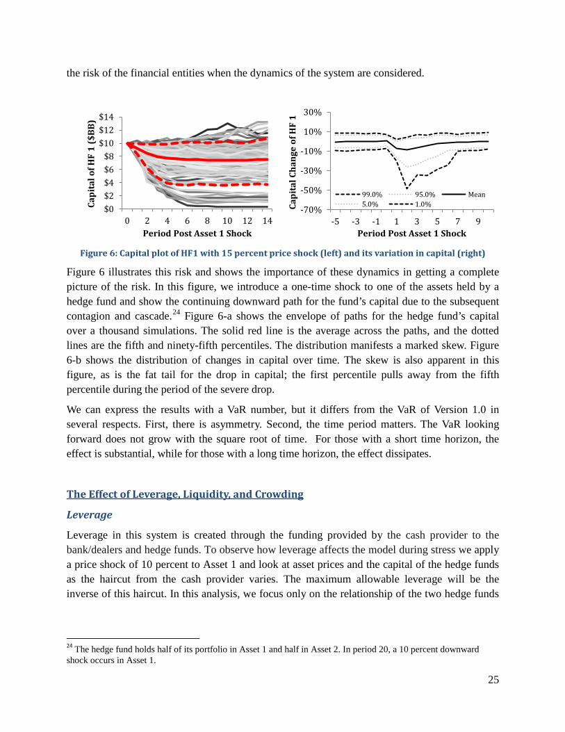
the risk of the financial entities when the dynamics of the system are considered.
Figure 6: Capital plot of HF1 with 15 percent price shock (left) and its variation in capital (right)
Figure 6 illustrates this risk and shows the importance of these dynamics in getting a complete picture of the risk. In this figure, we introduce a one-time shock to one of the assets held by a hedge fund and show the continuing downward path for the fund’s capital due to the subsequent contagion and cascade.24 Figure 6-a shows the envelope of paths for the hedge fund’s capital over a thousand simulations. The solid red line is the average across the paths, and the dotted lines are the fifth and ninety-fifth percentiles. The distribution manifests a marked skew. Figure 6-b shows the distribution of changes in capital over time. The skew is also apparent in this figure, as is the fat tail for the drop in capital; the first percentile pulls away from the fifth percentile during the period of the severe drop.
We can express the results with a VaR number, but it differs from the VaR of Version 1.0 in several respects. First, there is asymmetry. Second, the time period matters. The VaR looking forward does not grow with the square root of time. For those with a short time horizon, the effect is substantial, while for those with a long time horizon, the effect dissipates.
The Effect of Leverage, Liquidity, and Crowding
Leverage
Leverage in this system is created through the funding provided by the cash provider to the bank/dealers and hedge funds. To observe how leverage affects the model during stress we apply a price shock of 10 percent to Asset 1 and look at asset prices and the capital of the hedge funds as the haircut from the cash provider varies. The maximum allowable leverage will be the inverse of this haircut. In this analysis, we focus only on the relationship of the two hedge funds
24 The hedge fund holds half of its portfolio in Asset 1 and half in Asset 2. In period 20, a 10 percent downward shock occurs in Asset 1.
$0$2$4$6$8
$10$12$14
0 2 4 6 8 10 12 14
Capi
tal o
f HF
1 ($
BB)
Period Post Asset 1 Shock
-70%
-50%
-30%
-10%
10%
30%
-5 -3 -1 1 3 5 7 9
Capi
tal C
hang
e of
HF
1
Period Post Asset 1 Shock
99.0% 95.0% Mean5.0% 1.0%
26
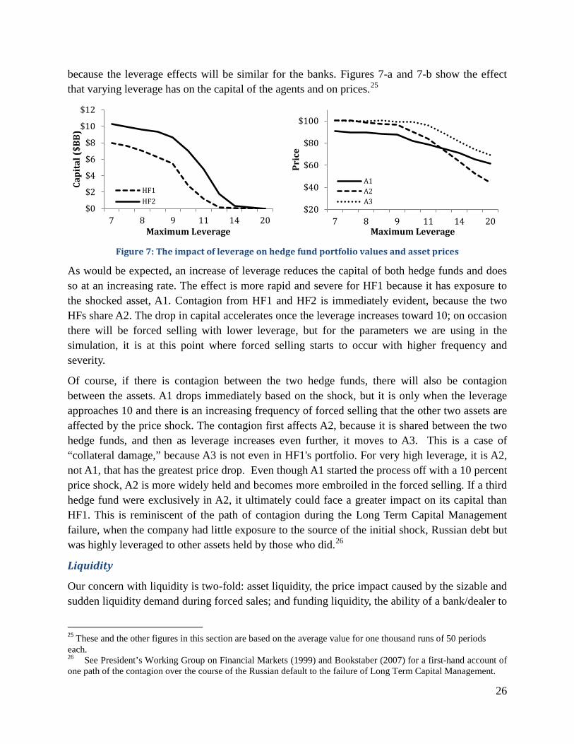
because the leverage effects will be similar for the banks. Figures 7-a and 7-b show the effect that varying leverage has on the capital of the agents and on prices.25
Figure 7: The impact of leverage on hedge fund portfolio values and asset prices
As would be expected, an increase of leverage reduces the capital of both hedge funds and does so at an increasing rate. The effect is more rapid and severe for HF1 because it has exposure to the shocked asset, A1. Contagion from HF1 and HF2 is immediately evident, because the two HFs share A2. The drop in capital accelerates once the leverage increases toward 10; on occasion there will be forced selling with lower leverage, but for the parameters we are using in the simulation, it is at this point where forced selling starts to occur with higher frequency and severity.
Of course, if there is contagion between the two hedge funds, there will also be contagion between the assets. A1 drops immediately based on the shock, but it is only when the leverage approaches 10 and there is an increasing frequency of forced selling that the other two assets are affected by the price shock. The contagion first affects A2, because it is shared between the two hedge funds, and then as leverage increases even further, it moves to A3. This is a case of “collateral damage,” because A3 is not even in HF1's portfolio. For very high leverage, it is A2, not A1, that has the greatest price drop. Even though A1 started the process off with a 10 percent price shock, A2 is more widely held and becomes more embroiled in the forced selling. If a third hedge fund were exclusively in A2, it ultimately could face a greater impact on its capital than HF1. This is reminiscent of the path of contagion during the Long Term Capital Management failure, when the company had little exposure to the source of the initial shock, Russian debt but was highly leveraged to other assets held by those who did.26
Liquidity
Our concern with liquidity is two-fold: asset liquidity, the price impact caused by the sizable and sudden liquidity demand during forced sales; and funding liquidity, the ability of a bank/dealer to
25 These and the other figures in this section are based on the average value for one thousand runs of 50 periods each. 26 See President’s Working Group on Financial Markets (1999) and Bookstaber (2007) for a first-hand account of one path of the contagion over the course of the Russian default to the failure of Long Term Capital Management.
$0
$2
$4
$6
$8
$10
$12
7 8 9 11 14 20
Capi
tal (
$BB)
Maximum Leverage
HF1HF2
$20
$40
$60
$80
$100
7 8 9 11 14 20
Pric
e
Maximum Leverage
A1A2A3

27
replace external funding with cash-equivalents in the event of a drop in funding. We model asset liquidity through beta-price, which measures the market impact of forced sale events. We model the funding liquidity by the liquidity ratio, which is the ratio of liquid (cash-equivalent) assets to short-term, nondurable funding.
Figure 8: The cross market impact of asset liquidity on hedge fund portfolio values and asset price
In Figure 8, we show the effect of variations in asset liquidity on capital and prices in the face of a 10 percent shock to A1. Lower liquidity has the same effect as higher leverage. The shock has a larger impact on the capital of both hedge funds, as well as on the average decline of prices, even showing that the impact of A2 is the greatest when there is large erosion in liquidity.
In Figure 8, all assets are assumed to have the same liquidity. The model allows the liquidity of each asset to be specified separately, and so a more complete analysis requires us to look at the joint affects across the various combinations of liquidity.
For the analysis of funding liquidity, the liquidity ratio has a role similar to the leverage ratio in the sense that there is a threshold for the liquidity ratio where a bank/dealer is forced to liquidate its inventory of assets; though there is a maximum leverage, there is a minimum liquidity ratio. Lower liquidity is bad; the creditworthiness of a bank/dealer is affected when the liquidity ratio drops below the minimum threshold.
The bank/dealer’s liquidity ratio can drop below the targeted value when it uses some reserves to finance assets it cannot liquidate as a result of the max-liquidation constraint. Beyond that, the bank/dealer uses its liquidity reserves to finance assets until it can liquidate them in the following periods.
Figure 9 presents results for the effect of variations in the liquidity ratio, where the liquidity ratio is assumed to be the same for both bank/dealers. The cells of each matrix to the left shows the capital of BD1 and the matrix to the right shows the price of A1 for various values of its liquidity ratio and its max-liquidation constraint.
$0
$2
$4
$6
$8
$10
$12
0 0.5 1 1.5 2
Capi
tal (
$BB)
Price Impact Factor
HF1HF2
$20
$40
$60
$80
$100
0 0.5 1 1.5 2
Pric
e
Price Impact Factor
A1A2A3

28
Figure 9:The impact of market liquidity constraints and liquidity ratios on prices and bank/dealer
portfolios
As would be expected, both a lower max-liquidation quantity and a lower liquidity ratio adversely affect the capital. The increased forced selling then results in a decrease in asset prices. It is interesting to note that for low levels of max-liquidity, the relationship between the liquidity ratio and capital is convex, and for high levels it is concave.
Crowding
The results shown above for leverage and liquidity are based on an equal allocation between A1 and A2 for HF1. We can see in Figure 10 the effect of crowded trades by varying the asset allocation from this benchmark for a given pricing shock. We do this by having HF2 hold 50 percent of its allocation in A2 and then see the effect of varying the proportion of the remaining 50 percent allocation held in A1 versus A3. In this analysis, we have A2 suffer the shock. As would be expected, a high allocation in A1 versus A3 leads to a larger price effect for A1 and A2, and a larger drop in capital for HF1 and HF2. However, as HF2 transfers its allocation from A3 to A1, the sensitivity to the allocations of HF2 affects both firms, though by different amounts.
Figure 10: : The effect of crowded trades due to varying asset allocations during a pricing shock
The greater the overall concentration in the shocked asset, the greater the effect will be to those
0 0.15
0.3 $-
$3
$5
$8
$10
0.5 1.5 2.5 3.5 4.5Max-Liquidity ($BB)
BD1 Capital ($BB)
0 0.15
0.3 $50
$60 $70 $80 $90
$100
0.5 1.5 2.5 3.5 4.5Max-Liquidity ($BB)
Asset 1 Price
$-
$2
$4
$6
$8
$10
0% 10% 20% 30% 40% 50%
Capt
ial (
$MM
)
Allocation of HF2 in A1
HF1HF2
$50
$60
$70
$80
$90
$100
0 0.1 0.2 0.3 0.4 0.5
Pric
e
Allocation of HF2 in A1
A1A2

29
who are holding that asset. A high allocation in A1 versus A2 leads to a larger price effect for A1 and a large drop in capital for HF1.
We can also look at crowded trades in non-shocked assets. We do this by varying the asset allocation of A2 when a shock occurs to A1. Figure 11 shows that the contagion effect to HF2 is larger when HF1 holds a large allocation in A1, while HF2 holds a large allocation in A2. This occurs because HF1 only starts to affect A2 as it moves into forced sale mode, and that only happens if it is highly exposed to A1 when the shock in A1 occurs. The same effect is true for A2; its price decline is greater the greater the allocation of HF1 in A1 and of HF2 in A2. Put another way, as the figure shows, the contagion effect is low when HF1 has little exposure to A1 and when HF2 has little exposure to A2.
Figure 11: The contagion effect to HF2 is larger when HF1 holds a large allocation in A1 while HF2
holds a large allocation in A2
5. Conclusion
This paper develops an agent-based model that gives a broad view of the transformations and dynamic interactions in the financial system, and in doing so, provides an avenue toward risk management Version 3.0, highlighting and monitoring key crisis dynamics, such as fire sales and funding runs. The model treats explicitly the various agents and their behavior rules during periods of crisis. Using a map of funding and collateral flows, it treats the link between the asset market and these essential elements of a crisis, modeling in detail the effect of the agents’ actions on each.
The model can be put to task in a number of areas:
Assess vulnerabilities in the financial system. The most immediate application of this model is along the evolutionary path from conventional stress tests, assessing the effect of shocks and detecting vulnerabilities, but now doing so as the shocks run their course through the system,
10%
50%
90%
$6
$7
$8
$9
$10
10% 30% 50% 70% 90%HF1 Allocationf of A1
HF2 Capital ($BB)

30
understanding the dynamic, knock-on effects.
Provide a “weather service.” Another task for the model, as events gather steam, is to assess what areas of the financial system are on the hurricane’s path; how bad the storm will be, and how long it will last.
Policy analysis. For policy planning, a goal of the model is to animate the path of various policy actions through the financial system, helping to determine the most effective points to place the emergency shut-off valves.
Assess data needs. The agent-based model also may find a role in demonstrating the value of new data sources and motivating data acquisitions. For example, the model can be run with constructed data and subsets of the data removed to see the degradation in its results.
Encourage liquidity providers. On a more tactical level, a possible application for the model is to help investors assess investment opportunities that are available as a liquidity provider in the face of a fire sale event. Taking the other side of the forced sale not only presents a profit opportunity; by stemming the spread of a crisis it might do so while providing great social value.
This paper presents a first step toward creating an operational model. Remaining tasks include identifying the important agents in the financial system and refining the decision rules for those agents; amassing the necessary data; and calibrating the model. The biggest challenge is in amassing the data to make an agent-based model operational. For practical application, an agent-based model can be made increasingly detailed based on how refined the data are. For example, there are agent-based models for traffic analysis that model each of hundreds of thousands of vehicles. In finance, there are models that treat each of thousands of mortgage holders as distinct agents, tracking not only the characteristics of their mortgages, but demographic data and income characteristics based on the zip codes where they are located.27 The model represented here is far from that level of refinement, and the immediate data challenges are more along the lines of data accessibility than data management. In terms of data requirements, the three key areas are exposures, especially for dominant investment themes that might relate to areas of crowding, as well as credit exposures; funding size, sources, durability and collateral; and “big trade” market liquidity, that is liquidity when outsized demand hits the market. The exposure and funding behind fire-sale events builds and changes slowly, so real time data is not necessary. Furthermore, a shock and resulting dynamic of systemic import is not going to occur in a subtle way; the exposures and related funding are likely to be large and broadly held.
27 See Geanakoplos et. al (2012).

31
Appendix I Equation Glossary
𝝋𝑪𝑪 Global parameter that governs the impact of Bank/Dealer 𝑘 going below 𝐿𝑖𝐿𝑅𝑇𝑡𝑖𝑇 𝑀𝑖𝑛 on its 𝐶𝐶𝑘
𝝋𝑯𝑪 Global parameter that governs the impact of Bank/Dealer 𝑘 going below 𝐿𝑖𝐿𝑅𝑇𝑡𝑖𝑇 𝑀𝑖𝑛 on its 𝐻𝐶𝑐,𝑘
𝑨𝒏 Assets held by Bank/Dealer or Hedge Fund 𝑛
𝑨𝒏𝑨𝑨𝑨𝑨𝑨𝑨𝑨𝑨𝑨𝒏 Vector of % of assets 𝑚 allocation for Bank/Dealer 𝑘 or Hedge Fund 𝑛
𝑨𝒏𝑻𝑨𝑻𝑻𝑻𝑨 Target quantity of assets held by Bank/Dealer 𝑘 or Hedge Fund 𝑛
𝜷𝒎 Price elasticity of demand for asset 𝑚
𝑪 The number of Cash Provider in the model
𝑪𝑨𝒌,𝑪𝑨𝒏 Collateral of Bank/Dealer 𝑘 or Hedge Fund 𝑛
𝑪𝑨𝒌𝑯𝑯 Collateral of Hedge Funds using Bank/Dealer 𝑘
𝑪𝑨𝒌𝑷𝑷 Collateral of Prime Broker of Bank/Dealer 𝑘
𝑪𝑨𝒌𝑻𝑻 Collateral of Trading Desk of Bank/Dealer 𝑘
𝑪𝑨𝑪𝒏 Capital of Bank/Dealer 𝑘 or Hedge Fund 𝑛
𝑪𝑪𝑲−𝟏 Credit exposure of Bank/Dealer 𝑘 to another Bank/Dealer 𝐾 − 1
𝑪𝑪𝒌𝑻𝑨𝑨𝑨𝑨 Credit exposure of Bank/Dealer 𝑘 to all the other Bank/Dealers
𝑪𝑪𝒌 Creditworthiness of Bank/Dealer 𝑘
𝑪𝑻𝑬𝒏 Funding driven sales of Bank/Dealer 𝑘 or Hedge Fund 𝑛
𝑯𝒏 Funding to Bank/Dealer 𝑘 or Hedge Fund 𝑛
𝑯𝒌𝑷𝑷 Funding to Prime Broker of Bank/Dealer 𝑘
𝑯𝒌𝑻𝑻 Funding to Trading Desk of Bank/Dealer 𝑘
𝑯𝑪𝑨,𝒌 The haircut Cash Provider 𝑐 give to Bank/Dealer 𝑘
𝑲 The number of Bank/Dealers in the model
𝑳𝑨,𝒌 Loan Cash Provider 𝑐 gives to Bank/Dealer 𝑘
𝑳𝑨,𝒌𝑴𝑨𝑴 Loan maximum of Cash Provider 𝑐 for Bank/Dealer 𝑘
𝑳𝑨,𝒌𝑻𝑨𝑻𝑻𝑻𝑨 Loan target of Cash Provider 𝑐 for Bank/Dealer 𝑘
𝑳𝑻𝑳𝒏𝑷𝑩𝑩𝑩𝑻𝑻 Leverage buffer of Bank/Dealer 𝑘 or Hedge Fund 𝑛
𝑳𝑻𝑳𝒏𝑪𝑩𝑻𝑻𝑻𝒏𝑨 Current leverage of Bank/Dealer 𝑘 or Hedge Fund 𝑛
𝑳𝑻𝑳𝒏𝑴𝑨𝑴 Leverage maximum of Bank/Dealer 𝑘 or Hedge Fund 𝑛
𝑳𝑻𝑳𝒏𝑻𝑨𝑻𝑻𝑻𝑨 Leverage target of Bank/Dealer 𝑘 or Hedge Fund 𝑛
𝑳𝑻𝑳𝒏𝑷𝑩𝑩𝑩𝑻𝑻 𝑹𝑨𝑨𝑻 Percent of 𝐿𝐸𝐿𝑛𝑀𝑇𝑀 that Bank/Dealer or Hedge Fund 𝑛 sets 𝐿𝐸𝐿𝑛
𝐵𝐵𝐵𝐵𝑅𝑅 to

32
𝑳𝑻𝑳𝒏𝑻𝑨𝑻𝑻𝑻𝑨 𝑹𝑨𝑨𝑻 Percent of 𝐿𝐸𝐿𝑛
𝐵𝐵𝐵𝐵𝑅𝑅 that Bank/Dealer or Hedge Fund 𝑛 sets 𝐿𝐸𝐿𝑛𝑇𝑇𝑅𝑅𝑅𝑡
to
𝑳𝑨𝑳𝒅𝑻𝒅𝑨𝑨 Liquidity reserve debit
𝑳𝑨𝑳𝒌𝑹 Liquidity reserve of Bank/Dealer 𝑘
𝑳𝑨𝑳𝒌𝑹𝑨𝑨𝑻 Liquidity reserve rate of Bank/Dealer 𝑘
𝑳𝑨𝑳𝒌𝑹𝑨𝑨𝑨𝑨 Liquidity ratio of Bank/Dealer 𝑘
𝑳𝑨𝑳𝒌𝑹𝑨𝑨𝑨𝑨𝑴𝑨𝒏 Liquidity ratio minimum of Bank/Dealer 𝑘
𝑳𝑨𝑳𝒌𝑹𝑨𝑨𝑨𝑨𝑻𝑨𝑻𝑻𝑻𝑨 Liquidity target of Bank/Dealer 𝑘
𝑴 The number of assets in the model
𝑵 The number of Hedge Funds in the model
𝑵𝒌 The subset of 𝑁 Hedge Funds that Prime Broker of Bank/Dealer 𝑘 works with
𝑶𝒏,𝒎(𝑨) Sum of all normal orders for buying or selling assets by Bank/Dealer 𝑘 or Hedge Fund 𝑛
𝑷𝒎 Price of asset 𝑚
𝑷𝑳𝒎 Previous day’s trading profit/loss accounting
𝑷𝑹𝒎 Price return for asset 𝑚
𝑷𝑹𝒎𝑹 Random price movement which is 𝑁(0,𝜎𝑚)
𝑸𝒏,𝒎 Quantity of asset 𝑚 held by Bank/Dealer 𝑘 or Hedge Fund 𝑛
𝑸𝒌𝑴𝑨𝑴 Quantity of assets that a Bank/Dealer 𝑘 can sell in a single period
𝑨 The period in which the model is currently in

33
References
Acemoglu, D., Ozdaglar, A., and Tahbaz-Salehi, A. (2013). Systemic Risk and Stability in Financial Networks, Working Paper 18727, National Bureau of Economic Research, Cambridge, Massachusetts.
Adrian, Tobias and Hyun Song Shin (2010). Liquidity and Leverage, Journal of Financial Intermediation, 19 (3), pp. 418-437
Adrian, Tobias and Hyun Song Shin (2014). Procyclical Leverage and Value-at-Risk, Review of Financial Studies, 27 (2), pp. 373-403.
Aguiar, Andrea, Richard Bookstaber, and Thomas Wipf (2014). A Map of Funding Durability and Risk, Office of Financial Research Working Paper No. 14-03.
Alfaro, Rodrigo, and Mathian Drehmann (2009). Macro Stress Tests and Crises: What Can We Learn? BIS Quarterly review, pp. 29-41.
Allen, F., and Babus, A. (2009). Networks in Finance. In The Network Challenge: Strategy, Profit, and Risk in an Interlinked World (eds. P. Kleindorfer, Y. Wind & R. Gunther), Wharton School Publishing, Upper Saddle River, New Jersey.
Battiston, S., Puliga, M., Kaushik, R., Tasca, P., and Caldarelli, G. (2012). Debtrank: Too entral to Fail? Financial Networks, the Fed and Systemic Risk. Scientific Reports 2, No. 541.
Bech, Morten L. and Enghin, Atalay (2008). The Topology of the Federal Funds Market, FRBNY Staff Report No. 354
Becher, Christopher, Millard, Stephen and Soramäki, Kimmo (2008), The Network Topology of CHAPS Sterling, Bank of England Working Paper No. 355.
Bisias, Dimitrios, Mark Flood, Andrew W. Lo, and Stavros Valavanis (2012). A Survey of Systemic Risk Analysis, Office of Financial Research Working Paper No. 1.
Bookstaber, Richard (2007). A Demon of Our Own Design, Wiley, New York.
Bookstaber, Richard (2012). Using Agent-Based Models for Analyzing Threats to Financial Stability, Office of Financial Research Working Paper No. 3.
Bookstaber R., Cetina, J., Feldberg, G., Flood, M., and Glasserman, P. (2014). Stress Tests to Promote Financial Stability: Assessing Progress and Looking to the Future, Office of Financial Research Working Paper No. 10.
34
Brunnermeier, Marcus and Lasse Pedersen (2005). Predatory Trading, Journal of Finance 60 (4), pp. 1825 - 1863.
Brunnermeier, Markus and Lasse Pedersen (2009). Market Liquidity and Funding Liquidity,i Review of Financial Studies, 22, pp. 2201-2238.
Brunnermeier, Markus and Yuliy Sannikov (2012). A Macroeconomic Model with a Financial Sector, National Bank of Belgium Working Paper No. 236.
Cont, Rama, Amal Moussa, and Edson B. Santos April (2013). Network Structure and Systemic Risk in Banking Systems, in: JP Fouque & J Langsam (eds.): Handbook of Systemic Risk, Cambridge University Press, pp. 327-368.
Degryse, H. and Nguyen, G. (2007). Interbank exposures: An Empirical Examination of Contagion Risk in the Belgian Banking System, International Journal of Central Banking, pp. 123-171.
Duffie, Darrell (2010). Presidential Address: Asset Price dynamics with Slow-Moving Capital, Journal of Finance 65 (4) pp. 1237 - 1267.
Farmer, D., M. Gallegati, C. Hommes, A. Kirman, P. Ormerod , S. Cincotti6, A. Sanchez, and D. Helbing. (2012). A Complex Systems Approach to Constructing Better Models for Managing Financial Markets and the Economy. The European Physical Journal Special Topics, 214, pp. 295-324.
Farmer, J. Doyne, and John Geanakoplos (2009). The Virtues and Vices of Equilibrium and the Future of Financial Economics, Complexity 14, pp. 11-38
Farmer, D., P. Patelli, and I. I. Zovko, (2005). The Predictive Power of Zero Intelligence in Financial Markets. Proceedings of the National Academy of Science, vol. 102, pp. 2254-2259, (2005).
Fostel, Anna and John Geanakoplos (2008). Leverage Cycles and The Anxious Economy, American Economic Review 98:4, pp. 1211-1244.
Freixas, X., Parigi, M., and Rochet, J. (2000). Systemic Risk, Interbank Relations and Liquidity Provision by the Central Bank, Journal of Money Credit and Banking, 32(3), pp. 611-638.
Geanakoplos, John, Robert Axtell, J. Doyne Farmer, Peter Howitt, Benjamin Conlee, Jonathan Goldstein, Matthew Hendrey, Nathan M. Palmer, and Chun-Yi Yang, (2012). Getting at Systemic Risk via an Agent-Based Model of the Housing Market. American Economic Review 102:3, pp. 53-58.

35
Ghoulmie, F., R. Cont, and J-P Nadal, (2005). "Heterogeneity and Feedback in an Agent-based Market Model," Journal of Physics: Condensed Matter, Vol. 17, pp. 1259-1268.
Gorton, G. (2010). Slapped in the Face by the Invisible Hand, Oxford University Press.
Greenwood, R., Augustin Landier, and David Thesmar (2012). Vulnerable Banks. NBER Working Paper No. 18537.
International Monetary Fund (2008). Iceland: Financial System Stability Assessment Update. IMF Country Report No. 08/368. Washington: IMF.
Iori, Giulia, de Masi, Giulia, Precup, Ovidiu, Gabbi, Giampaolo and Caldarelli, Guido (2008). A Network Analysis of the Itaian Overnight Money Market, Journal of Economic Dynamics and Control, Vol. 32(1), pp. 259‐ 278.
LeBaron, B. A Builders Guide To Agent-Based Financial Markets, Quantitative Finance, 1, pp:254261 (2001a)
LeBaron, B. "Evolution of Time Horizons in an Agent-Based Stock Market," Macroeconomic Dynamics, 5, pp. 225-254. (2001b)
LeBaron, Blake. "Agent-based Computational Finance." Handbook of Computational Economics. vol. 2 Ed. Tesfatsion and Judd. North-Holland, 2006. 1187-1232.
Lux, T. and M. Marchesi. "Scaling and Criticality in a Stochastic, Multi-Agent Model of a Financial Market." Nature 397: 498-500. (1999)
Maslov, S. Simple Model Of A Limit Order-Driven Market, Physica A, 278, pp: 571-578. (2000)
Montagna, M. and Kok, C. (2013) Multi-layered Interbank Model for Assessing Systemic Risk, Kiel Institute Working Paper No. 1873.
Palmer, R.G., W. Brian Arthur, John H. Holland, Blake LeBaron, Paul Tayler.(1994). Artificial Economic Life: A Simple Model Of A Stock Market, Physica D, 75, pp: 264-274.
Preis, T., S. Golke, W. Paul and J. J. Schneider. (2006). Multi-Agent Based Order Book Model of Financial Markets, Europhysics Letters, 75 (3), pp. 510-516.
The Report of the President’s Working Group on Financial Markets (1999).
Shleifer, A., and Vishny, R. (2011). Fire Sales in Finance and Economics, Journal of Economic Perspectives, pp. 25, 29–48.

36
Song, Rui, Sowers, Richard and Jones, Jonathan (2014). The Topology of Central Counterparty Clearing Networks and Network Stability, Stochastic Models, 30 (1), pp. 16-47.
Soramäki, Kimmo, Bech, Morten, Jeffrey, Arnold, Glass, Robert J. and Beyeler, Walter E. (2007). The Topology of Interbank Payment Flows, Physica A, 379, pp. 317‐ 333.
Upper, C. and Worms, A. (2004). Estimating bilateral exposures in the German interbank market: Is there a danger of contagion?, European Economic Review, 48(4), pp.:827-849.
von Peter, G (2007). International Banking Centres: a Network Perspective, BIS Quarterly Review, December, pp. 33-45.
Wetherilt, Anne, Zimmerman, Peter and Soramäki, Kimmo (2010). The Sterling Unsecured Loan Market During 2006-08: Insights from Network Theory, Bank of England Working Paper No. 398.


![Revised Financial Results for Sept 30, 2015 (Standalone) [Result]](https://img.pdfslide.us/doc/110x75/577ca6a51a28abea748bf62b/revised-financial-results-for-sept-30-2015-standalone-result.jpg)


![Revised Financial Results for Sept 30, 2015 [Result]](https://img.pdfslide.us/doc/110x75/577c78451a28abe0548f5a8d/revised-financial-results-for-sept-30-2015-result.jpg)