CCB 3033 ADVANCED TRANSPORT PROCESSES CBB 3033 TRANSPORT PHENOMENA

COMPUTATIONAL FLUID

DYNAMICS (CFD) LABORATORY

Instruction Manual

Energy Transport

2

COMSOL TUTORIAL 2a: HEAT TRANSFER (1 hour) Consider a cylindrical heating rod which is sheathed by a concentric tube of thickness 0.05

m. The entire assembly is immersed in a fluid and the system is at steady-state, as shown

below. We wish to determine the temperature distribution within the sheath. The temperature

of the heater is constant at 400K. The temperature at R1 is the same as the temperature of the

heater, 400K. The fluid temperature is constant at 300K surrounding sheath at R2. Length of

R2 = 2R1

The geometry of the solid sheath illustrated in 3D is shown below

400oK

300oK

Copper

3

>> Open the COMSOL 4.0 software

MODEL WIZARD

1) In the Space Dimension, select the 3D coordinate system given for the geometry. Click the next button

2) In the Add Physics, choose Heat Transfer> Heat Transfer in Solids(ht). Click the plus button to add. Then, click next button

1

2

2

1

3

4

3) In the Select Study Type, we click on stationary study, then click the finish button

GEOMETRY

Build Cylinder 1

1) In Model Builder, right click on geometry tab and choose the cylinder

1

2

5

2) Let us specify the dimension of the Cylinder 1, then click on build selected

Build Cylinder 2

3) Repeat step 1 and 2, then specify the dimension of the Cylinder 2 as the following figure below

1

2

3

1

2

3

6

Boolean Operation : Difference

4) Under Model Builder> Untitle.mph> Model> Geometry 1 tab, right click on Geometry 1 and select Boolean Operations> Difference

5) Under Settings> Difference> Objects to add, select the Cylinder 1 and click plus button to add the object

1

2 3

7

6) Under Settings> Difference> Objects to subtract, click activate selection button

7) Then, select the Cylinder 2, click plus button to add the object and click build selected button

The completed geometry is according to the following figure

1

2 3

8

MATERIAL

1) In Model Builder, right click and choose Open Material Browser

2) In Material Browser> Materials> Built-in, select Copper, right click on it and select Add Material to Model

3) Select Body 1 (whole body) for geometry scope. Make sure density, heat capacity and thermal conductivity in material content have been filled automatically

9

PHYSICS

1) Under Model Builder> Untitle.mph> Model> Heat Transfer tab, right click on Heat Transfer tab and select Temperature to assign the Temperature 1

Temperature 1 Boundaries : 400o K

2) Select boundary 4, 5, 7, and 8(whole face inside). After selection, we specify temperature as following figure

1

2 3

4

10

Temperature 2 Boundaries : 300o K

3) Repeat step 1 to assign the Temperature 2. Select boundary 1, 2, 3, 6, 9, and 10. Then, define temperature as in following figure

MESH

1) Find Mesh 1> size then click. We specify the element size as figure below

1

2 3

4

11

2) 2) Right click on Mesh 1 tab and click Free Triangular. Then, we click build selected button

Therefore, the mesh of the model is defined by the following figure

12

COMPUTE AND DATA PLOT

1) Under Model Builder> Untitle.mph> Study 1 tab, right click on it and select compute. Thus, the contour of the model is defined by the following figure

3D plot group 1 : Surface Temperature Contour in 3D Isometric View

3D plot group 2 : Slice Contour of Temperature

13

Arrow Vector

1) Under Model Builder> Untitle.mph> Results tab, right click on 3D Plot Group 2 and select Arrow Volume

2) Under Settings> Expression click right click on 3D Plot Group 2. Then, find and click replace expression button, select Heat Transfer> Total heat flux

1

2

3

14

3) Under Settings> Coloring and Style, we fill the scale factor and the color as below. Then, click plot button

Therefore, the arrow of heat direction is define by following figure

Slice Contour of Temperature with Arrow Vectors

1

2

15

Line Graph : Radial Temperature Distribution in z-direction

1) To make vertical line in z-direction in the middle of model (x=0.15m), right click on the Results>Data Sets tab and choose Cut Line 3D. Then, specify the x-axis, y-axis, and z-axis coordinate as below

2) To make a line plot, right click on Results and choose 1D Plot Group. Then, right click on Results>1D Plot Group 3 and choose Line Graph

3) Find the Data set and choose Cut Line 3D 1

4) Change X-Axis to Z-Coordinate

Thus, line graph of Z-Coordinate vs Temperature is given by following figure

16

Line Graph : Horizontal Temperature Distribution in x-direction

1) To make horizontal line in the middle of model (y=0.075m), repeat the steps for Line graph for Vertical line. Right click on the Results>Data Sets tab and choose Cut Line 3D. Then, specify the x-axis, y-axis, and z-axis coordinate as below

2) To make a line plot, right click on Results and choose 1D Plot Group. Then, right click on Results>1D Plot Group 3 and choose Line Graph

3) Find the Data set and choose Cut Line 3D 2

4) Change X-Axis to X-Coordinate

Thus, line graph of X-Coordinate vs Temperature is given by following figure

17

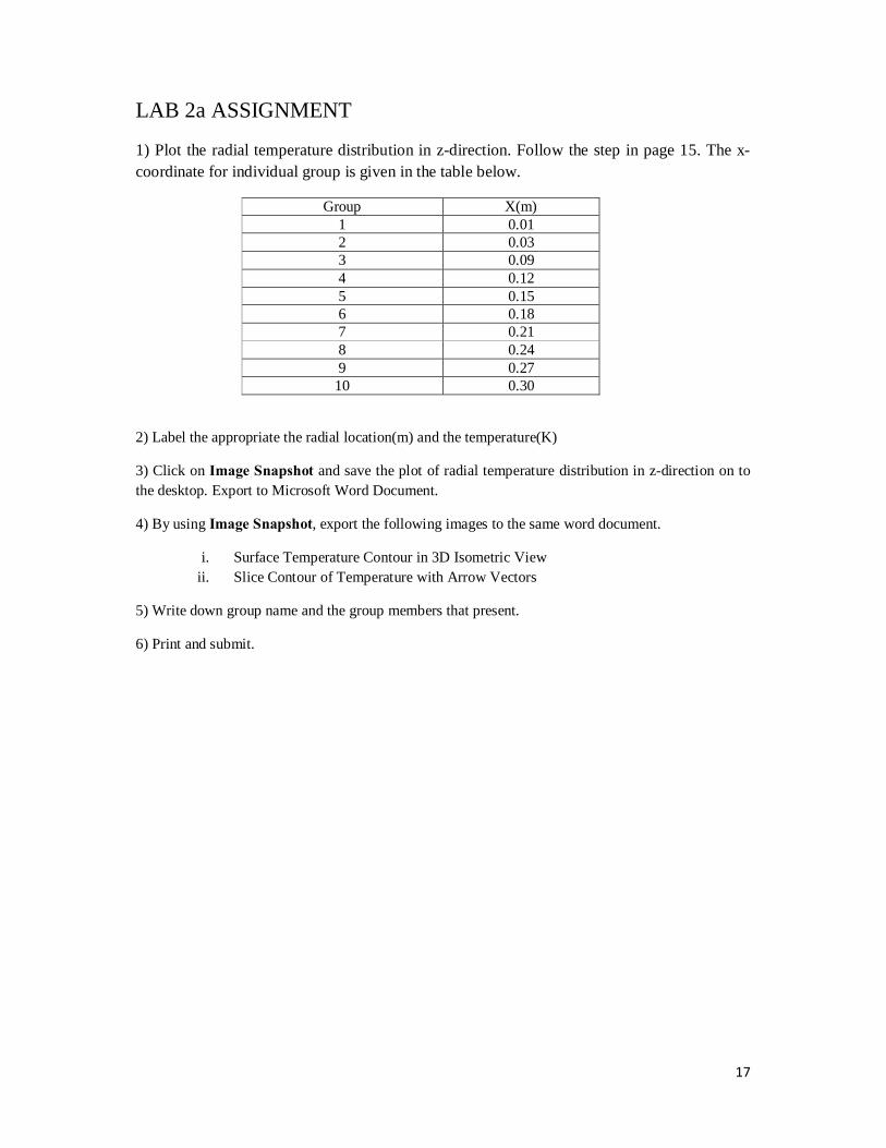
LAB 2a ASSIGNMENT

1) Plot the radial temperature distribution in z-direction. Follow the step in page 15. The x-coordinate for individual group is given in the table below.

Group X(m) 1 0.01 2 0.03 3 0.09 4 0.12 5 0.15 6 0.18 7 0.21 8 0.24 9 0.27

10 0.30

2) Label the appropriate the radial location(m) and the temperature(K)

3) Click on Image Snapshot and save the plot of radial temperature distribution in z-direction on to the desktop. Export to Microsoft Word Document.

4) By using Image Snapshot, export the following images to the same word document.

i. Surface Temperature Contour in 3D Isometric View ii. Slice Contour of Temperature with Arrow Vectors

5) Write down group name and the group members that present.

6) Print and submit.

18

COMSOL TUTORIAL 2b: HEAT TRANSFER (1 hour) Consider an air flows through the cylindrical hollow heating rod which is Q = 1,000 W/m3.

The air has velocity 0.1 m/s and the temperature of air is constant at 300K. Please model and

predict the temperature of air after passing 0.25 m the cylindrical rod.

The geometry of the solid sheath illustrated in 3D is shown below

Air

Copper Rod

19

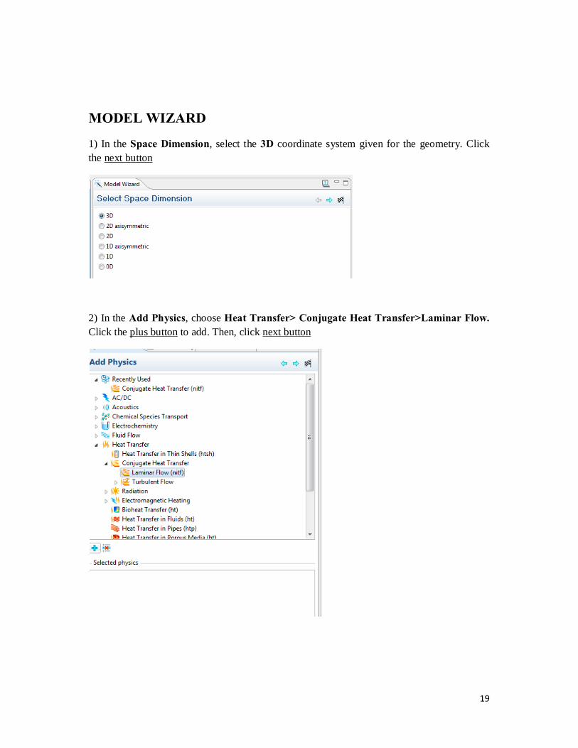
MODEL WIZARD

1) In the Space Dimension, select the 3D coordinate system given for the geometry. Click the next button

2) In the Add Physics, choose Heat Transfer> Conjugate Heat Transfer>Laminar Flow. Click the plus button to add. Then, click next button

20

3) In the Select Study Type, we click on stationary study, then click the finish button

GEOMETRY

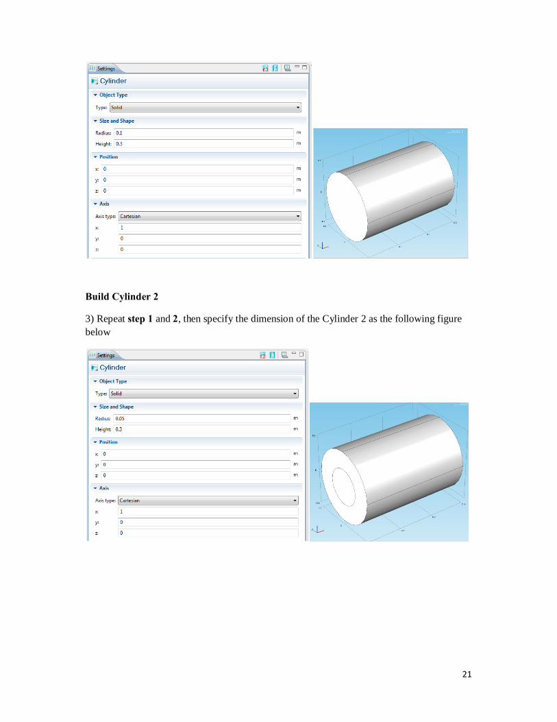
Build Cylinder 1

1) In Model Builder, right click on geometry tab and choose the cylinder

2) Let us specify the dimension of the Cylinder 1, then click on build selected

21

Build Cylinder 2

3) Repeat step 1 and 2, then specify the dimension of the Cylinder 2 as the following figure below

22

Build Block 1

4) In Model Builder, right click on geometry tab and choose the block

5) Let us specify the dimension of the Block 1, then click on build selected

23

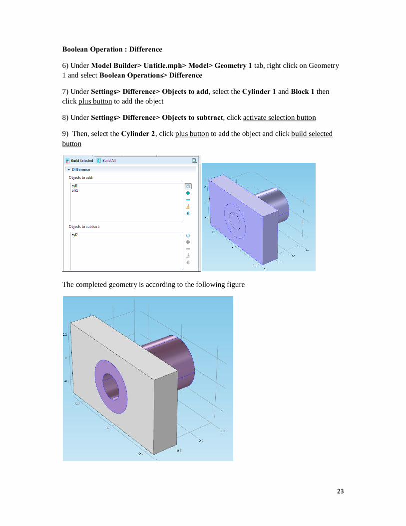
Boolean Operation : Difference

6) Under Model Builder> Untitle.mph> Model> Geometry 1 tab, right click on Geometry 1 and select Boolean Operations> Difference

7) Under Settings> Difference> Objects to add, select the Cylinder 1 and Block 1 then click plus button to add the object

8) Under Settings> Difference> Objects to subtract, click activate selection button

9) Then, select the Cylinder 2, click plus button to add the object and click build selected button

The completed geometry is according to the following figure

24

MATERIAL

Copper selection

1) In Model Builder, right click and choose Open Material Browser

2) In Material Browser> Materials> Built-in, select Copper, right click on it and select Add Material to Model

3) Select rod cylinder for geometry scope. Material content have been filled automatically

25

Air Selection

4) Follow step no.1

5) In Material Browser> Materials> Built-in, select Air, right click on it and select Add Material to Model

6) Select Block for geometry scope. Material content have been filled automatically

26

PHYSICS

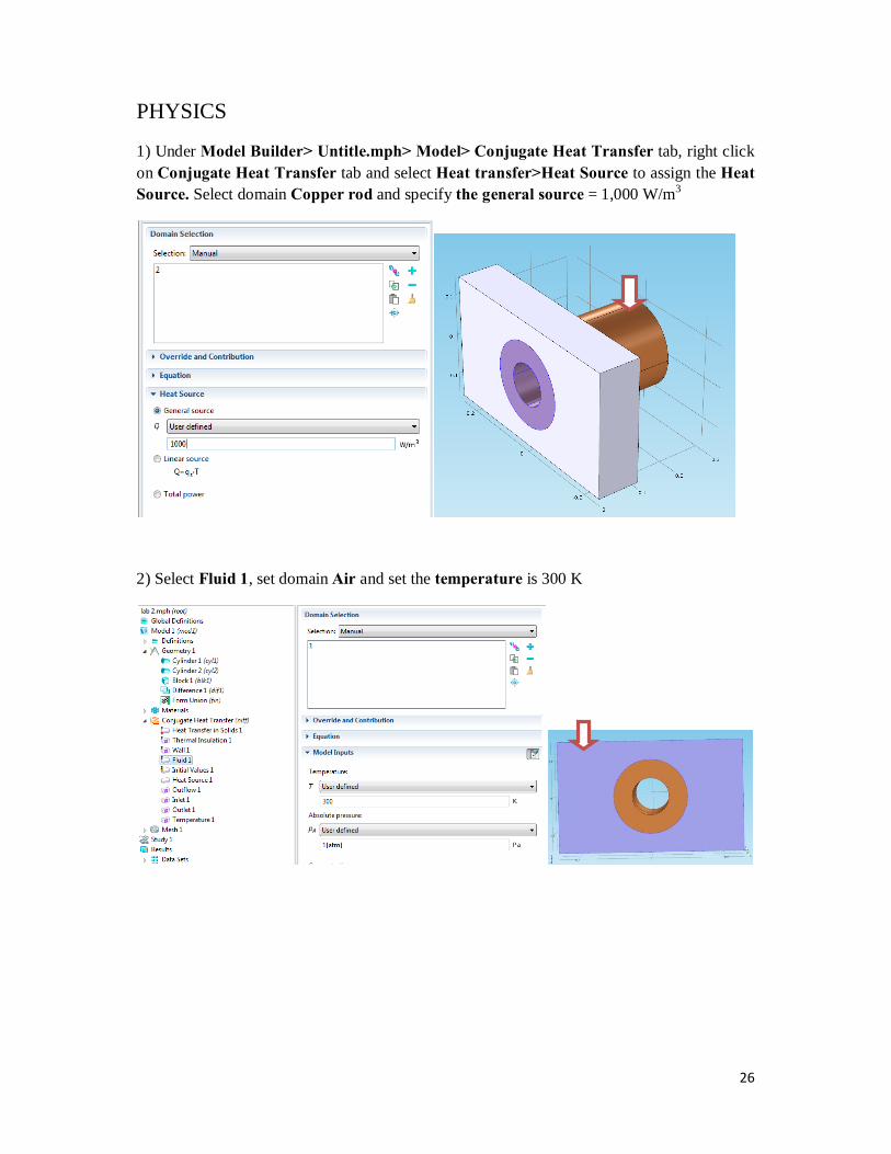
1) Under Model Builder> Untitle.mph> Model> Conjugate Heat Transfer tab, right click on Conjugate Heat Transfer tab and select Heat transfer>Heat Source to assign the Heat Source. Select domain Copper rod and specify the general source = 1,000 W/m3

2) Select Fluid 1, set domain Air and set the temperature is 300 K

27

3) Right click on Conjugate Heat Transfer tab and select Heat transfer>Outflow to assign the Outflow. Select boundary : surface number 2

4) Right click on Conjugate Heat Transfer tab and select Laminar Flow>Outlet to assign the Outlet. Select boundary : surface number 2 and set pressure is 0

28

5) Right click on Conjugate Heat Transfer tab and select Laminar flow>Inlet to assign the Inlet. Select boundary : surface number 14 and specify velocity is 0.1 m/s

6) Right click on Conjugate Heat Transfer tab and select Heat Transfer>Temperature to assign the Temperature of air from inlet. Select boundary : surface number 14 and specify temperature is 300 K

29

MESH

1) Find Mesh 1> size then click. We specify the element size as figure below

2) Right click on Mesh 1 tab and click Free Triangular. Then, we click build selected button

Therefore, the mesh of the model is defined by the following figure

30

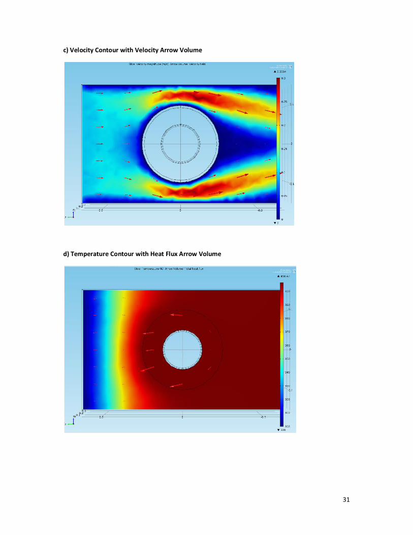
COMPUTE & RESULT

1) Under Model Builder> Untitle.mph> Study 1 tab, right click on it and select compute. Thus, the contour of the model is defined by the following figure

a) Velocity magnitude contour

b) Temperature Contour

31

c) Velocity Contour with Velocity Arrow Volume

d) Temperature Contour with Heat Flux Arrow Volume

32

LAB ASSIGNMENT 2b 1) Please Change the value of Heat Source

Group Q (W/m3) 1 10 2 50 3 100 4 200 5 500 6 800 7 1200 8 1500 9 2000

10 2500

2) Click on Image Snapshot a, b, c, d

4) Predict the temperature in the outlet and give conclusion

5) Write down group name and the group members that present.

6) Print and submit.