INSTREAM WOOD TRANSPORT, AND EFFECTS OF FOREST HARVEST ON

GEOMORPHOLOGY AND FISH, IN NORTHERN MINNESOTA STREAMS

A DISSERTATION SUBMITTED TO THE FACULTY OF THE GRADUATE SCHOOL

OF THE UNIVERSITY OF MINNESOTA BY

ERIC CHRISTOPHER MERTEN

IN PARTIAL FULFILLMENT OF THE REQUIREMENTS FOR THE DEGREE OF

DOCTOR OF PHILOSOPHY

JACQUES FINLAY AND HEINZ STEFAN, ADVISERS

JUNE 2009

© Eric Christopher Merten 2009

i

ACKNOWLEDGEMENTS

First and foremost, I thank my family for keeping me both grounded and motivated. I

couldn’t have asked for better officemates.

Jacques Finlay and Heinz Stefan have been excellent advisers, helping me with the wood

project and with all aspects of my PhD. My committee was very involved throughout the

process; Lucinda Johnson, Ray Newman, and Bruce Vondracek provided my initial

funding and got my projects rolling.

Many other people helped with my projects; they are acknowledged or coauthors in the

chapters that follow. I had the opportunity to work with colleagues both new and old

during my PhD, and I look forward to ongoing collaboration. Financial support is

acknowledged in each chapter; I benefitted from two teaching assistantships as well.

I am grateful to all.

ii

ABSTRACT

Trees provide critical functions to the ecology of streams. Trees affect hydrology,

mitigate sediment inputs, and buffer water temperatures by providing shade. Watersheds

with a higher proportion of mature forest tend to have less variable hydrographs, and

older trees provide larger pieces of wood to streams. Instream wood itself affects nearly

every process in stream ecology.

Despite their ecological importance, trees and instream wood have been greatly

modified by humans. The studies described in this dissertation advance current

knowledge as follows:

We demonstrate that headwater streams in northern forests can require ten years

to recover from a large input of fine sediment, depending on the occurrence of

stormflows.

Our analyses suggest that, at the basin scale, warmer air temperatures in summer

are more important to the abundances of some headwater fish species than instream

habitat or spring precipitation. The analyses also lend support to previous findings that

riparian forest harvest can cause local stream warming.

Wood transport in streams is a dynamic process. Forty-one percent of over 800

wood pieces were mobilized (at least 10m) during a study period by a single high flow

event. Thirty-two percent of the mobilized pieces became entrapped again before leaving

their study reach.

Mobilization of wood in streams is a complex function of both mechanical and

hydraulic factors. Eleven potential predictor variables were studied, and seven were

iii

identified as significant to wood mobilization using multiple logistic regression. The

seven predictors were burial, effective depth, length ratio, bracing, rootwad presence,

downstream force ratio, and draft ratio.

Entrapment of wood in streams is related primarily to the length ratio and weight

of the wood pieces. The mechanisms for entrapment are not always clear; wood pieces

may simply be entrapped wherever they are located when high water recedes.

Together, this dissertation suggests that forest harvest should avoid excess

sediment inputs (due to persistence) and stream warming (due to effects on fish). It also

develops models that can be used for more informed management of instream wood.

Stream managers and restorers can apply the results presented to reverse the impacts of

historic logging and wood removal on streams.

iv

TABLE OF CONTENTS

ACKNOWLEDGEMENTS……………………………………………………….……….i

ABSTRACT…………………………………………………………………………..…..ii

TABLE OF CONTENTS……………………………………………………….…….......iv

LIST OF TABLES……………………………………………..…………………..…….vii

LIST OF FIGURES………………………………………….………..…………….........ix

OVERVIEW AND SUMMARY OF RESULTS………...…………………….…………1

CHAPTER 1: Relationship of sediment dynamics in moraine, headwater streams in

northern Minnesota to forest harvest..……………………………….……………6

Summary..…………………………………………………………………………………8

Introduction………………….…………………………………………………………….9

Study area…………………...……………………………………………………………11

Methods…………………...……………………………………………………………...12

Results ………………………………………………………………………………...….16

Discussion………………………………………………………………………..………17

Conclusion………………………………………………………………………...……..20

Acknowledgements……………………………………………………………...……….21

Tables and figures………………………………………………………………..………23

CHAPTER 2: Relations between fish abundances, summer temperatures, and forest

harvest in a northern Minnesota stream system from 1997 to 2007…………......30

Summary..…………………………………………………………………………….….32

Introduction……………………………………………………………………….…..….33

v

Methods…………………………………………………………………………………..37

Results ……………………………………………………………………………………41

Discussion………………………………………………………………………………..43

Conclusion……………………………………………………………………………….48

Acknowledgements………………………………………………………………………48

Tables and figures…………………………………………………………………..……50

CHAPTER 3: Factors influencing wood mobilization in Minnesota streams…………..58

Summary..………………………………………………………………...……………...60

Introduction…………………………………………………………………...………….61

Forces acting on wood pieces in a stream and potential mobilization predictors………..64

Methods…………………………………………………………………………...……...73

Results …………………………………………………………………………...……….84

Discussion……………………………………..…………………………………….…...92

Conclusion……………………………………………………………………………….98

Acknowledgements……………………………..………………………….…………….99

CHAPTER 4: Entrapment of wood in Minnesota streams determined by a length ratio

and weight………………………………………………………………...…….100

Summary..…………………………………………..………………………………..…102

Introduction and background………………………..…………………………...……..103

Mechanisms for entrapment…………………………………………………………….107

Field data collection…………………………………………………………………….112

Data analysis methods………………………………………………………….……….119

vi

Results …………………………………………………………………….…………….120

Discussion………………………………………………………………………………127

Conclusion……………………………………………………………………...………131

Acknowledgements……………….…………………………………………………….132

BIBLIOGRAPHY………………………………………………………………………133

APPENDIX A: List of symbols …….…………………………………………………162

APPENDIX B: Calculating submerged volume and area normal to flow…..…………163

APPENDIX C: Histograms of data from 858 pieces of wood evaluated in this study...170

APPENDIX D: Histograms of data from 344 pieces of wood evaluated in this study..175

vii

LIST OF TABLES

Table 1-1. Watershed area for each study stream, open or young forest area, and the area

of harvested plots……………………..………………………………….………23

Table 1-2. Channel characteristics (slope, width, mean depth), sediment particle sizes,

and tree basal area in the riparian management zone one year after forest

harvest……………………………………………………………………....……24

Table 1-3. Basin-scale year effects for canopy cover, unstable banks, embeddedness, and

surficial fine substrates in streams from 1997 (pre-harvest) to 2007 (ten years

post-harvest) using repeated measures ANOVAs………………………..………25

Table 2-1. Yearly average IBI score, total fish abundance, and mean number of fish by

species per 50-m reach, based on calculated abundance estimates…………...…50

Table 2-2. Yearly average values for all reaches for the proportion of fine substrates,

large wood, estimated summer water temperature, and total spring

precipitation……………………………………………………………………...51

Table 2-3. Coefficients of determination (r2) for IBI scores and fish abundances in

relation to the proportion of fine substrates, large wood, summer air temperature,

or total spring precipitation at the basin scale……………………………………52

Table 3-1. Variables measured or calculated for each piece of wood…………………...78

Table 3-2. Mean and standard deviation for wood piece characteristics in summer 2007,

and geomorphic and hydraulic stream characteristics during peak discharges in

fall 2007…………………………………………………………………….……85

viii

Table 3-3. Mean and standard deviation for geomorphic and hydraulic characteristics for

each study site during the peak discharges in fall 2007………………………….86

Table 3-4. Variables retained in the final model for mobilization……………………….87

Table 4-1. Variables measured or calculated……………………………………..…….116

Table 4-2. Mean and standard deviation for characteristics of wood pieces and 10-m

stream sections at the nine study reaches……………………………....……….122

Table 4-3. Mean and standard deviation for hydraulic and geomorphic characteristics for

each study site during peak discharges in fall 2007……………………...……..122

Table 4-4. Variables retained in the final model for entrapment…………………….....123

ix

LIST OF FIGURES

Figure 1-1. Pokegama Creek system showing riparian plots (numbered), stream channels

and tributaries, roads, and beaver impoundments…………………………….….26

Figure 1-2. (A) Canopy cover remained high in 1998 the year after harvest, declined in

1999 and 2000 from windthrow, and recovered in 2006. (B) Unstable banks

increased in the 3 years after harvest but recovered by 2006. (C) Embeddedness

increased after harvest and remained high, (D) as did the proportion of surficial

fine substrates………………………………………………………………...…..27

Figure 1-3. (A) Residual pool depth was reduced by sand deposits after the pre-harvest

1997 measurement, (B) depth of refusal increased through all sampling periods

until after a large storm in November 2007……………………………...………28

Figure 1-4. Comparison from 2007 for Pfankuch Channel Stability Ratings against (A)

proportion of surficial fine substrates, (B) embeddedness, (C) residual pool depth,

and (D) depth of refusal………………………………………………...…….….29

Figure 2-1. Study sites located near Grand Rapids, Minnesota, USA………...…………53

Figure 2-2. Rank abundance curves for fish species across all sites………………….....54

Figure 2-3. Mean summer air temperatures for June through August 1997 through

2007………………………………………………………………………………55

Figure 2-4. The relationship between mean summer air temperature from June through

August and the IBI scores and abundance (annual mean for all 50-m reaches in

the basin) of brook trout, northern redbelly dace, and brook stickleback……..…56

x

Figure 2-5. Mean August temperature just downstream of each site minus the mean

August temperature just upstream of each site (i.e., stream warming) by harvest

treatment and year………………………………………………………..………57

Figure 3-1. Draft of a floating piece of wood, shown in cross-section…………..………66

Figure 3-2. Plan view of channel with pieces of wood oriented perpendicular to the flow

and parallel to the flow……………………………………………………..……68

Figure 3-3. Side view of channel illustrating pieces of wood pitched parallel to the stream

bed and at 45° to the stream bed………………………………………………....69

Figure 3-4. Study sites (stars with arrows) along the north shore of Lake Superior in

Minnesota………………………………………………………………...………74

Figure 3-5. Number of stream bed transects by dominant substrate for the nine

streams………………………………………………………………………..….75

Figure 3-6. Hydrograph for the Poplar River from June to November 2007…………....76

Figure 3-7. Plan view of stream channel illustrating lateral positions of trees (open

circles) large enough to brace a floating piece of wood…………………………80

Figure 3-8. Side view of stream channel illustrating a piece of wood suspended above the

water surface……………………………………………………………………..82

Figure 3-9. Expected probability of mobilization as a function of the effective depth,

length ratio, downstream force ratio, or draft ratio…………………………...….90

Figure 3-10. Frequency of bracing of wood pieces in relation to the object on which the

piece was braced in summer 2007…………………………………………….....92

Figure 4-1. Draft of a floating piece of wood in a stream cross-section………………..105

xi

Figure 4-2. Study sites (stars with arrows) along the north shore of Lake Superior in

Minnesota………………………………………………………………….……113

Figure 4-3. Number of stream bed transects by dominant substrate, for the nine streams

sampled…………………………………………………………………………114

Figure 4-4. Hydrograph for the Poplar River during the study period from June to

November 2007…………………………………………………………………114

Figure 4-5. Plan view of channel illustrating lateral positions of trees (open circles) large

enough to brace a floating piece of wood………………………………………118

Figure 4-6. Expected probability of entrapment as a function of the length ratio, weight,

or branching complexity………………………………………………………..126

Figure 4-7. Numbers of new pieces found in 2008 in three stream reaches, according to

location or manner in which pieces were braced……………………………….127

1

OVERVIEW AND SUMMARY OF RESULTS

Streams have been modified worldwide by logging and wood removal. The

relationship between trees, dead wood and stream ecology is very strong, and many

adverse effects of logging and wood removal have been observed. As described below,

this dissertation addresses gaps in the current knowledge of the relationship between

trees, wood and streams to further aid in stream protection and restoration.

The first two chapters of this dissertation examine effects of riparian forest

harvest on streams in the Pokegama Creek system near Grand Rapids, Minnesota, over an

11-year study period. Previous studies in other watersheds have related forest harvest to

increased stream discharge, increased inputs of fine sediment, decreased inputs of leaf

litter and wood, community shifts in aquatic biota, and warmer stream temperatures in

summer. We examined effects of experimental forest harvest (2 to 11% of the

watersheds) using existing data from 1997 (pre-harvest) to 2000 (four years post-harvest)

and new data from 2006 and 2007. Most of our analyses were at the basin scale; we

pooled data from 33 50-m sample stream reaches for each of the six years studied.

The last two chapters examine natural wood transport in streams along the north

shore of Lake Superior in Minnesota using an extensive field dataset collected over a

two-year period. Natural pieces of wood provide a variety of ecosystem functions in

streams, including high quality habitat, organic matter retention, increased hyporheic

exchange flow and transient storage, and enhanced hydraulic and geomorphic

heterogeneity. Given the strong role that wood plays in streams, factors that influence

wood transport are therefore critical to the understanding of stream ecology. In previous

2

studies of wood transport the scope was typically constrained to a small number of

variables, or laboratory flumes were used, and wood was represented by dowels or

flumes. We tracked natural wood pieces in nine streams over distances up to 800m with a

resolution of 10m. Seven wood piece characteristics were measured and the location of

each piece was documented twice, and related to the hydraulic stream characteristics.

In the first chapter of the dissertation I examine the dynamics of fine sediment in

the Pokegama Creek system. Fine sediment can enter a stream channel by aeolian

deposition, overland flow, bank erosion or even landslides, or by delivery from roads, or

the disturbances created by forest harvest equipment. In a previous study a large input of

fine sediment to the Pokegama Creek system within the first year after experimental

forest harvest had been documented. We sought to extend the previous study using new

data (2006 to 2007) and unpublished historic data to examine the dynamics of fine

sediment over a longer time frame. Canopy cover, proportion of unstable banks, surficial

fine substrates, residual pool depth, and streambed depth of refusal were used as response

variables in repeated measured ANOVAs to test for basin-scale year effects. All response

variables showed significant basin-scale year effects, indicating differences between

years when considering all sites throughout the basin. The proportion of unstable banks

increased for several years post-harvest, coinciding with an increase in fine sediment in

the streams. An increase in unstable banks may have been caused by forest harvest

equipment, increased windthrow and exposure of rootwads, or increased discharge and

bank scour. Fine sediment in the channels had not recovered by summer 2007 (ten years

post-harvest), even though canopy cover and unstable banks had returned to 1997 levels.

3

After several storm events in fall 2007, fine sediment was flushed from the channels and

remaining sediment deposits returned to 1997 levels. Although our study design did not

discern the source of the initial sediment inputs (e.g., forest harvest, road crossings, other

natural causes), we could demonstrate that moraine, headwater streams can require high

stormflows to recover from large inputs of fine sediment.

In the second chapter of the dissertation I examine changes of the fish community

in the Pokegama Creek system. Pooling data from the study area for each year,

significant decreases in the index of biotic integrity and the abundance of brook trout and

northern redbelly dace over the study period were demonstrated. Abundance of brook

sticklebacks also decreased over time while creek chub abundance increased, although

neither trend was significant. We next related fish abundances between 1997 and 2007 to

instream habitat (fine substrates and large wood) and environmental conditions (summer

air temperature and spring precipitation) at the basin scale. It was determined that lower

“index of biotic integrity” scores were significantly related to warmer air temperatures, as

were lower abundances for brook trout, northern redbelly dace, and brook sticklebacks.

Fish variables were not significantly related to fine substrates in the streambed, large

wood, or total spring precipitation at the basin scale. Air temperatures increased only

~0.06° C/yr during the study period (consistent with regional estimates of climate

change), but water temperatures near harvest plots with thinned riparian tree cover were

warmer than those near plots with riparian buffers (based on an ANOVA using stream

temperatures measured in 2006 and 2007). We suggest that summer temperatures may

influence fish communities more than fine sediment, large wood, or spring precipitation

4

in forested headwater streams based on the basin-scale relationships from this study. The

removal of riparian vegetation exacerbates warming of streams by reduced shading.

The third chapter of the dissertation is an examination of mobilization of natural

wood pieces. Mobilization was defined as the displacement of a stationary piece of wood

by at least 10m. The characteristics and locations of 865 undisturbed wood pieces

(usually > 0.1 m in diameter for a portion > 1 m in length) were documented in summer

2007 in nine streams, each with a study reach 250 to 800 m long (4,190 m total). The

locations of the pieces were determined again in fall 2007 after an overbank stormflow

event. Hydraulic conditions in the streams during the entire study period were determined

using calibrated flow simulation (HEC-RAS) models. Eleven potential predictor variables

were studied, and seven were identified as significant to wood mobilization using

multiple logistic regression. The composition of the final model indicates that wood

mobilization under natural conditions is a complex function of both mechanical factors

(burial, length ratio, bracing, rootwad presence, draft ratio) and hydraulic factors

(effective depth, downstream force ratio). Although the study included only one

stormflow event, the nine streams exhibited a wide range of geomorphic and hydraulic

conditions. The model should be applicable to at least a similarly wide range of

conditions in other watersheds. The mobilization model can provide guidance to stream

management and stream restoration. For example, if stable pieces are a goal for stream

management then features such as partial burial, low effective depth, high length relative

to channel width, bracing against other objects (i.e., stream banks, trees, rocks, or larger

wood pieces), and rootwads are desirable.

5

The fourth chapter of my dissertation was an examination of wood piece

entrapment in a stream. Entrapment was defined to occur when a piece of wood comes to

rest after being transported at least 10 m. A total of 344 pieces met met the criterion for

entrapment, based on changes in locations before and after the fall 2007 overbank

stormflow event. The ratio of wood piece length to effective stream width was the most

important independent variable for entrapment; longer pieces are more likely to be

entrapped. Multiple logistic regression also showed that piece weight was the second-

most important variable for entrapment; heavier pieces are more likely entrapped.

The scaled resolution for the wood transport study was similar to that of flume

studies, and a wide natural range of wood piece and stream characteristics was examined.

The results can provide guidance to stream modifications where wood entrapment is

undesirable (e.g., at road crossings or other infrastructure); the effective stream width

required to pass particular wood pieces can be determined by the model. Conversely, the

results can be used to determine conditions that enhance entrapment where wood pieces

are valued for ecological functions. Entrapment remains difficult to predict in natural

streams, and often may simply occur wherever wood pieces are located when high water

recedes.

Stream managers and restorers can, if they so choose, apply the results from this

dissertation toward reversing the impacts of logging and wood removal on streams.

6

CHAPTER 1: Relationship of sediment dynamics in moraine,

headwater streams in northern Minnesota to forest harvest

Eric C. Merten

Department of Fisheries, Wildlife, and Conservation Biology and the Water Resources

Science Graduate Program, University of Minnesota, 1980 Folwell Ave, St. Paul,

Minnesota, 55108

Nathaniel A. Hemstad

Department of Biology, Inver Hills Community College, 2500 East 80th St, Inver Grove

Heights, Minnesota, 55076

Randall K. Kolka

USDA Forest Service, Northern Research Station, 1831 Hwy 169 East, Grand Rapids,

Minnesota, 55744

Raymond M. Newman

Department of Fisheries, Wildlife, and Conservation Biology, University of Minnesota,

1980 Folwell Ave, St. Paul, MN, 55108

7

Elon S. Verry

Ellen River Partners, Inc.

Grand Rapids, Minnesota, 55744

Bruce Vondracek1

USGS, Minnesota Cooperative Fish and Wildlife Research Unit1, University of

Minnesota, 1980 Folwell Ave, St. Paul, MN, 55108

Corresponding author: Eric C. Merten, 1-651-345-2867, 1-612-625-1263 (fax),

mert0042@umn.edu

Correspondence address: Eric C. Merten, Department of Fisheries, Wildlife, and

Conservation Biology, University of Minnesota, 1980 Folwell Ave, St. Paul, Minnesota,

55108

1 The Unit is jointly sponsored by the U. S. Geological Survey, the University of

Minnesota, the Minnesota Department of Natural Resources, and the Wildlife Management Institute

8

SUMMARY

Fine sediment can enter stream channels through a variety of mechanisms,

including aeolian processes, landslides, overland flow, bank erosion, delivery from roads,

or forest harvest. The persistence of fine sediment in streams, however, is less well

known. This study investigated the dynamics of fine sediment in four moraine, headwater

streams in north central Minnesota in relation to forest harvest. We examined the

dynamics of fine sediment from 1997 (pre-harvest) to 2007 (ten years post-harvest) at

study plots with upland clear felling and riparian thinning, using canopy cover,

proportion of unstable banks, surficial fine substrates, residual pool depth, and streambed

depth of refusal as response variables. Basin-scale year effects were significant (P <

0.001) for all response variables when evaluated by repeated measures ANOVAs.

Throughout the study area, the proportion of unstable banks increased for several years

post-harvest, coinciding with an increase in fine sediment. Increased unstable banks may

have been caused by forest harvest equipment, increased windthrow and exposure of

rootwads, or increased discharge and bank scour. Fine sediment in the channels did not

recover by summer 2007, even though canopy cover and unstable banks had returned to

1997 levels. After several storm events in fall 2007, ten years after the initial sediment

input, fine sediment was flushed from the channels and returned to 1997 levels. Although

our study design did not discern the source of the initial sediment inputs (e.g., forest

harvest, road crossings, other natural causes), we have demonstrated that moraine,

headwater streams can require an enabling event (e.g., high stormflows) in order to

recover from large inputs of fine sediment.

9

INTRODUCTION

The effects of fine sediment on stream ecosystems have been well documented,

and can include increased turbidity, reduced ability of aquatic organisms to feed, clogged

gills of fish and macroinvertebrates, smothered eggs and larvae, and homogenization of

habitats (Waters 1995, Sweka and Hartman 2001). Fine sediment can enter streams

through a variety of mechanisms, including aeolian processes, landslides, overland flow,

bank erosion, or delivery from roads (Chamberlin et al. 1991, Wondzell 2001,

Broadmeadow and Nisbet 2004). However, sediment inputs from aeolian processes are

minor in temperate forests (Steedman and France 2000), and landslides are uncommon in

streams with hillslopes under 35˚ (Johnson et al. 2007).

Forest harvest can also contribute excess sediment to streams; excess sediment

can manifest as increases in total suspended sediment (Gomi et al. 2005), streambed

aggradation (Keim and Schoenholtz 1999), or the proportion of surficial fine substrates

(Davies and Nelson 1994, Thompson et al. 2009). For example, suspended sediment

during stormflow events increased significantly in a Fiji catchment after salvage logging

and slash burning; much of the sediment was mobilized from new logging roads and

landing areas (Waterloo et al. 2007). Similarly, thinning only 11% of the standing timber

volume with horse skidding produced a significant increase in suspended sediment to a

stream in Turkey (Serengil et al. 2007a). Hydrographs also indicated significantly more

stormflow in both study areas (Waterloo et al. 2007, Serengil et al. 2007b).

An altered stream hydrograph can lead to increased bank erosion (Brooks et al.

1997), and may take decades to recover after forest harvest (Moore and Wondzell 2005).

10

In a forest harvest study in British Colombia, peak snowmelt discharge remained above

pre-harvest levels for the five-year duration of the study (Macdonald et al. 2003). Verry

(2004) noted that channel-forming flows double or triple after 60% of a catchment is

converted from forest to non-forest conditions in the upper Midwest; however, little work

has been done on the effect of elevated flows on sediment inputs.

Input processes aside, few studies have examined recovery of streams after large

inputs of sediment (Gomi et al. 2005). In one case, the bedload of fine sediment required

more than two years to return to natural levels after road-improvement activities

(Kreutzweiser and Capell 2001), and in another case sediment eroded from logging roads

and skid trails and was stored in stream channels for 3.4 years (Gomi et al. 2006). In a

review of available studies, Gomi et al. (2005) noted that sediment yield usually recovers

within one to six years post-harvest, barring landslides. Previous research in Minnesota

(Merten 1999, Hemstad and Newman 2006, Hemstad et al. 2008) suggests that levels of

fine sediment can increase significantly after forest harvest. However, more research is

needed to determine how long fine sediment will persist in channels.

Our objective was to evaluate changes in fine sediment in four headwater streams

following timber harvesting in riparian areas in the Sugar Hills moraine of north central

Minnesota. We predicted that fine sediment loading would increase after forest harvest,

but that sediment levels would return to pre-harvest conditions within 10 years. Hemstad

et al. (2008) suggested that basin-scale factors were more important than plot-level

factors to sediment in our study area. Although our study did not discern between

11

changes due to forest harvest, road crossings, or natural causes, it did evaluate recovery at

the basin scale after a large input of fine sediment.

STUDY AREA

Twelve study plots were located in the Pokegama Creek system in north-central

Minnesota (47º 8.039´N, 93º 37.405´W); the basin included four small, forested basins

with moraine hills rising five to seven meters above the valley floor and hillslopes of 1 to

30% (Fig. 1). One plot was on an intermittent tributary and was omitted from analyses.

Soils and parent material in the Sugar Hills moraine were loamy sands with gravel lenses

and cobble/boulder inclusions (Nyberg 1987). The upland soils were fertile and well-

drained, supporting late successional forests of sugar maple (Acer saccharum Marsh) and

basswood (Tilia americana Linnaeus). Early successional forests following clearcut

logging included: paper birch (Betula papyrifera Marsh), aspen (Populus tremuloides and

P. grandidenta) and balsam fir (Abies balsamea [Linnaeus] Miller). Riparian forests at

the floodplain elevation included black ash (Fraxinus nigra Marsh), along with sugar

maple and basswood and remnant early succession species (about 10% of basal area).

Riparian forests in 1997 averaged 30 m2/ha of basal area (Palik et al. 2003).

The drainage basins of the four study streams varied in size from 129 to 281 ha

(Table 1). Harvested study plots accounted for 2 to 11% of their respective basins,

whereas open areas or young forest (<16 years) in the catchment accounted for 25 to 49%

of their respective basin. The slope, width, and mean depth of the study streams were

measured at each plot location and reaches immediately upstream, along with tree basal

12

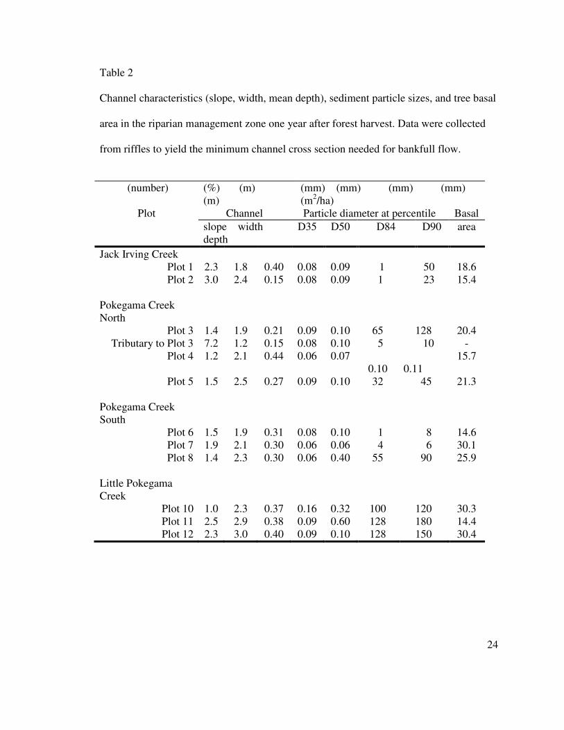
area in and above the plots (Table 2). Channel gradients were relatively steep (0.7 to

3.5%, one tributary was 7.2%) because they drained glacial moraine hills. Sediment in

the streams was predominately fine sand, as evidenced by the diameter of the 50th

percentile of all particles (D50). The substrate contained gravel and cobble sizes at the 84th

percentile (D84) where channels had a steeper gradient. Cobble and small boulders were

concentrated in the glacial drift of Little Pokegama Creek (Table 2). A paved road ran

approximately 250 m to the north and parallel to one stream (Pokegama Creek North),

and an existing gravel road with culverts crossed two of the streams (Pokegama Creek

North and Pokegama Creek South) just upstream from the study plots. Two additional

culvert crossings were farther upstream on Pokegama Creek North (Fig. 1). Beaver dams

and impoundments were present below the confluence of Pokegama Creek North and

Pokegama Creek South, and well upstream of plots 1 and 2 on Jack Irving Creek.

METHODS

Harvested study plots

Harvest treatments were replicated throughout the four basins. Harvest treatments

spanned the stream at each plot (4.9 ha, with 2.45 ha on each side of the stream) and

included: unharvested controls (N = 2), 30-m unharvested riparian buffer with the upland

clearcut (N = 3), or thinned to 12.3 m2/ha within a 30-m riparian strip with the upland

clearcut (N = 6). Trees were harvested in fall 1997 using either a cut-to-length harvester

paired with a forwarder or a feller-buncher paired with a grapple skidder (Palik et al.

2003). Pre-harvest data were collected in 1997 and post-harvest data were collected in

13

1998-2000 and 2006-2007. Each plot included 150 to 200 m of stream length, and plots

were ~200 m apart. Three reaches were sampled at each plot: 50 m immediately upstream

of the treatment, 50 m immediately downstream of the treatment, and within the

downstream 50 m of the plot (Fig. 1). Study plots were established collaboratively

(Merten 1999, Fox 2000, Fredrick 2003, Hanowski et al. 2003, Palik et al. 2003,

Hanowski et al. 2007, Hemstad et al. 2008).

Examination of year effects at study plots

A variety of data were collected at the study plots for examination of basin-scale

year effects (i.e., overall differences between years when considering all sites). Six

variables were measured to characterize stream bank and channel conditions: proportion

of unstable banks, canopy cover, surficial fine substrates, embeddedness, streambed

depth of refusal, and residual pool depth (Lisle 1987). Visual estimates of the proportion

of bank area that was unstable (not covered by vegetation, roots, or rocks) were made in

the three 50-m reaches at each plot (Merten 1999, Hemstad et al. 2008). The value for

each 50-m reach was the mean of three 17-m sections. Canopy cover was also determined

at the center of each 17-m section using a spherical concave forest densiometer in all four

directions (Lemmon 1957). Unstable banks and canopy cover were assessed in July

1997-2000 and 2006-2007.

Surficial substrates were examined in the three reaches at each of the 11 study

plots. Each 50-m reach at each plot was divided into five 10-m subreaches, to avoid

sampling substrates exclusively at the upstream or downstream end of a 50-m reach.

14

Seven circular quadrats (28 cm in diameter) were placed in random locations in each 10-

m subreach to visually estimate the percentage of sand, silt, or clay (i.e., fine substrates)

on the streambed surface (for a total of 1,155 quadrats per year). Embeddedness was

estimated in each quadrat as the degree to which larger substrates were buried in fine

substrates (e,g., a quadrat with cobbles half-buried in sand was 50% embedded, whereas

a quadrat with only fine substrates visible was 100% embedded). Surficial substrates

were examined in July 1997-2000 and 2006-2007.

Sediment storage in the channel was evaluated using depth of refusal and residual

pool depth. At each of the 11 study plots, the ten riffles with the largest substrates and the

ten deepest pools were sampled. Depth of refusal was determined at each riffle and pool

by probing with a rod to determine the thickness of the fine sediment layer (i.e., sand or

silt) in the stream channel. A tapered aluminum rod was used to probe the sediment. The

depth of refusal for each plot was the mean of the ten riffles and ten pools. Depth of

refusal was measured in summer 1997, 1998, 2006, and 2007. Residual pool depth (i.e.,

pool depths minus riffle depths) was determined for each plot in summer 1997, 2006, and

2007 with a laser level following Lisle (1987).

In fall 2007, rain events that totaled 112 mm above the August/September mean

for the study period caused high flows throughout the study area (Minnesota State

Climatology Office). Depth of refusal data were collected at all plots in November 2007

to investigate whether sediment had been flushed from the streams by these high flows.

Previous work documented short-term effects of forest harvest on sediment in the

Pokegama Creek system, and suggested that basin-scale effects were more important than

15

local-scale effects or harvesting technique (Hemstad et al. 2008). Therefore, year effects

were evaluated at all study plots, regardless of harvest treatment, using repeated measures

ANOVAs that included our new data from 2006-2007. Two factors were included in each

analysis: a factor for year and a blocking factor for the four streams. The blocking factor

was necessary to address a lack of independence between sampling units on the same

stream. Variables were transformed as needed to reduce heteroscadasticity and improve

normality. A repeated measures ANOVA was examined separately for canopy coverage,

unstable banks, embeddedness, and surficial fine substrates. In addition, repeated

measures ANOVAs were used to evaluate year effects on depth of refusal and residual

pool depth, using a year factor but no blocking factor (due to greater separation between

sampling units and lower replication). When ANOVAs were significant (P < 0.05),

Tukey’s HSD comparison was used to compare differences in mean values for the

response variable between years. The statistical software R was used for all analyses

(Ihaka and Gentleman 1996).

Comparisons with Pfankuch Channel Stability Rating

We compared our methods for assessing fine sediment to the Pfankuch Channel

Stability Rating (Pfankuch 1975), an established method for assessing geomorphic

stability. The rating uses qualitative categories for 15 metrics to describe conditions of

stream banks and channels, and sums the values into a score from 38 (the most stable

condition) to 152 (the most disturbed condition). In 2007 the Pfankuch Channel Stability

Rating was determined at each of the 12 study plots, and was compared with simple

16

regressions against our measures of surficial fine substrates, embeddedness, depth of

refusal, and residual pool depth (combining data from all three reaches at each plot).

RESULTS

Year effects at study plots

Canopy cover, unstable banks, embeddedness, and surficial fine substrates were

significantly different across years during the study period (Table 3). Although canopy

cover was unaffected by harvest itself (i.e., 1997 and 1998 were not significantly

different), canopy cover declined as a result of windthrow by 2000 and had recovered to

pre-harvest levels by 2006 (Fig. 2A). The proportion of unstable banks increased between

1997 and 2000, but had recovered by 2007 (Fig. 2B). Embeddedness increased from 1997

to 1998 and remained above pre-harvest levels through 2007 (Fig. 2C). Surficial fine

substrates also increased from 1997 to 1998, but partially recovered in 1999 after a heavy

summer storm (Fig. 2D). The proportion of surficial fine substrates again increased

significantly relative to pre-harvest levels in 2000 and 2006, but recovered in 2007.

Sediment storage was also significantly different across years during the study

period. Residual pool depths were shallower than pre-harvest conditions in both 2006 and

2007 (Fig. 3A). Depth of refusal was not significantly different between 1997 and 1998

but increased significantly between 1998 and 2006, and remained significantly greater

than pre-harvest levels in summer of 2007 (Fig. 3B). However, following heavy rains in

fall 2007 large amounts of freshly deposited sand were noted on the floodplains and

17

depth of refusal in November was no longer significantly different from pre-harvest

levels (Fig. 3B).

Comparisons with Pfankuch Channel Stability Rating

The Pfankuch Channel Stability Rating was correlated highly and positively with

the proportion of surficial fine substrates (R2 = 0.78, Fig. 4). The correlations with other

variables were weaker; the R2 for embeddedness, residual pool depth, and depth of

refusal were 0.4, 0.31, and 0.28.

DISCUSSION

Our study demonstrated that headwater streams in moraine landscapes may

require ten years to recover after a large input of fine sediment, depending on the rate of

stream bank revegetation and the frequency of large storm events. Our fine sediment

variables relate to overall channel stability; the proportion of surficial fine substrates

correlated particularly well with the Pfankuch Stream Channel Stability Rating, which

includes visual assessments of surficial conditions. Correlations were weaker for

embeddedness, depth of refusal, and residual pool depth, all of which assess the thickness

of the layer of fine sediment rather than surficial coverage. Embeddedness, depth of

refusal, and residual pool depth values remained significantly changed ten years after the

input of sediment between 1997 and 1998. The year effects we documented may be

related to changes in bank scour, windthrow, storm events, and damage from forest

harvest equipment.

18

Bank scour throughout the study area may have contributed fine sediment through

at least 2000, as evidenced by higher proportions of unstable banks. Banks were fully

revegetated by 2007, by which time bank scour was presumably reduced. Excess

sediment (i.e., embeddedness, depth of refusal, and residual pool depth) remained in the

streams through summer 2007. Storm events in fall 2007 led to high streamflows that

flushed enough sediment onto the floodplain to return depth of refusal values to 1997

conditions.

Local weather patterns can influence windthrow, sediment storage, and sediment

transport (Brooks et al. 1997). Storm events occurred during 1998 and 1999 (Minnesota

State Climatology Office), followed by a period through 2001 with no storm events when

sediment likely stayed in the channel. Heavy rainfall events occurred again in 2001-2005,

many caused by summer storms with high winds that may have caused windthrow and

inputs of associated sediment (Grizzel and Wolff 1998). Another period followed from

2006 through mid-2007 when sediment likely remained in the channel, until the storms of

fall 2007 led to sediment deposition onto the floodplains. The analysis of decade-long

studies should be interpreted in the context of such weather cycles.

Windthrow along the channel banks (Hemstad et al. 2008) may also have led to

increases in unstable banks and channel sediment (Grizzel and Wolff 1998). Rootwads

exposed by windthrow influenced channel morphology in places by adding associated

sediment, partially blocking the channel, and inducing bank cutting around the rootwad.

Studies of windthrow in riparian buffers in the upper Midwest are rare (Heinselman 1955,

Heinselman 1957, Elling and Verry 1978) but suggest that windthrow rates are greatest

19

near the edge of buffers (sensu Martin and Grotefendt [2007]), thus wider buffers protect

streamside trees from windthrow.

High discharge may also have contributed to the increases in unstable banks and

channel sediment. The streams in the Pokegama Creek system may have experienced

increases in bankfull discharge due to increases in water yield from harvested areas

(Verry 2004, Brooks et al. 1997, Macdonald et al. 2003, Detenbeck et al. 2005, Moore

and Wondzell 2005, Waterloo et al. 2007). Although the harvested percentages of the

four basins were only 2 to 11%, Serengil et al. (2007b) found hydrologic effects after

11% of a basin was harvested. Lower thresholds may simply be precluded by the

accuracy of hydrologic measurements (Verry 1986). Hemstad et al. (2008) found few

plot-level effects of forest harvest in the Pokegama Creek system from 1997-2000, but

suggested that basin-scale changes may have masked impacts at the plot level. Hemstad

and Newman (2006) also found few plot-level effects in the Knife River basin in

northeast Minnesota, but observed basin-scale increases in unstable banks and surficial

fine substrates 0-2 years after forest harvest. It is noteworthy that the greatest changes in

surficial fine substrates and embeddedness during the study period occurred immediately

after forest harvest, indicating a possible response to altered hydrology or soil disturbance

from harvesting equipment.

Small tributary channels, if impacted by harvesting equipment, can also contribute

to sediment loading in mainstem channels. Study plot 3 contained a small, yet steep

(7.2%) intermittent tributary 1.2 m wide and 15 cm deep that was crossed repeatedly with

harvesting equipment (sensu unrestricted harvest treatment of Keim and Schoenholtz

20

[1999]). The machine traffic broke down the banks and razed the intermittent channel. In

subsequent years the channel was reformed by bankfull discharges, delivering large

amounts of fine sand into the mainstem of Pokegama Creek North. The pool in

Pokegama Creek North just below the confluence of the tributary was nearly filled with

sediment (89% loss of cross sectional area) and mean depth was reduced by 82% (E.

Verry, unpubl. data). Use of a temporary bridge at a designated crossing site on the

intermittent tributary would likely have preserved channel dimensions and prevented

sediment delivery to the mainstem channel. Minnesota’s voluntary guidelines for forest

harvest now recommend such crossings for intermittent channels as well as perennial

channels (MFRC 2005).

CONCLUSION

Previous research has shown that headwater streams can be negatively impacted

by fine sediment following riparian logging and concomitant changes in land use in the

catchment (Kreutzweiser and Capell 2001, Gomi et al. 2005, Hemstad et al. 2008).

Although our study did not discern between changes due to forest harvest, road crossings,

or natural causes, we evaluated recovery after a large input of fine sediment. Our study

demonstrated that moraine, headwater streams can require an enabling event (e.g., high

stormflows) in order to recover from large inputs of fine sediment. Although study plots

were relatively small (4.9 ha) and retained some riparian trees, we observed basin-scale

year effects for fine sediment in the stream channels that are consistent with forest

harvest effects documented elsewhere (Gomi et al. 2005).

21

Some recommendations may help mitigate loading of fine sediment following

forest harvest. First, we concur with others (e.g., Brooks et al. 1997, Verry 2004,

Detenbeck et al. 2005) that it is wise to minimize alterations to hydrology and bank scour

by reducing the percentage of the basin that is harvested. Second, impacts of roads and

crossings should be minimized, such as by preventing machine traffic within a riparian

buffer (Keim and Schoenholtz 1999, Lacey 2000). When crossings are necessary, erosion

control measures should be taken and bridge spans or culverts should be large enough to

accommodate stormflows without causing backwater effects or hydraulic contraction

(Johnson 2002). Similarly, harvesting and forwarding around and across intermittent

stream channels should use temporary bridges at designated crossing points to protect the

stream banks (MFRC 2005). Our third recommendation is to manage riparian areas for

sustainable stocks, where the annual growth increment exceeds the losses due to

windthrow. Forests, and streams, can provide a variety of products and ecological

services (Neuman 2007). Continued research on the linkages between forest harvesting

and sedimentation can allow more informed decisions about forest management.

ACKNOWLEDGMENTS

This work was funded by the Minnesota Department of Natural Resources

Division of Fisheries, the Minnesota Forest Resources Council, the National Council for

Air and Stream Improvement, the U.S. Forest Service, the Minnesota Environment and

Natural Resources Trust Fund, and Minnesota Trout Unlimited. Charlie Blinn and Brian

Palik selected the study plots and supervised the manipulations. John Hansen and Jim

22

Marshall of UPM-Kymenne Corporation Blandin provided access to the study plots.

Forest harvest was completed by Rieger Logging. We sincerely thank the following for

assistance with data collection: Andy Arola, Brenda Asmus, Jason Bronk, Rebecca

Bronk, Ryan Carlson, Bill Coates, Jacquelyn Conner, Carrie Dorrance, Art Elling,

MaryKay Fox, Jo Fritz, Sarah Harnden, Deacon Kyllander, Marty Melchior, Steffen

Merten, Mateya Miltich, Brittany Mitchell, Erik Mundahl, Elliot Nitzkowski, Ian Phelps,

Lisa Pugh, Jeff Rice, David Schroeder, Jeremy Steil, Dustin Wilman, and Jason

Zwonitzer. The Statistical Consulting Service at the University of Minnesota provided R

code for analysis. Comments from Jacques Finlay, Heinz Stefan, and two anonymous

reviewers improved the quality of the manuscript.

23

TABLES AND FIGURES

Table 1

Watershed areas for each study stream, open or young forest area, and the area of

harvested plots. Areas are based on 1977 and 2003 air photos with on-site reconnaissance

in 1997. Open areas include road rights of way, harvested riparian plots, and other

harvest areas with trees less than 16 years old in the watershed.

(ha) (ha) (ha) (%) (ha) (%)

Total 1977 open

2003 open

2003 open

Study plots

Harvest plots

Harvest plots

Jack Irving 281 99.8 138.5 49 1, 2 4.8 2 Pokegama North 168 23.7 42.8 25 3, 4, 5 11.7 7 Pokegama South 135 52.6 62.8 47 6, 7, 8 7.9 6 Little Pokegama 129 14.8 23.8 18 9, 10,11,

12 13.7 11

24

Table 2

Channel characteristics (slope, width, mean depth), sediment particle sizes, and tree basal

area in the riparian management zone one year after forest harvest. Data were collected

from riffles to yield the minimum channel cross section needed for bankfull flow.

(number) (%) (m) (m)

(mm) (mm) (mm) (mm) (m2/ha)

Plot Channel Particle diameter at percentile Basal

slope width depth

D35 D50 D84 D90 area

Jack Irving Creek

Plot 1 2.3 1.8 0.40 0.08 0.09 1 50 18.6 Plot 2 3.0 2.4 0.15 0.08 0.09 1 23 15.4

Pokegama Creek North

Plot 3 1.4 1.9 0.21 0.09 0.10 65 128 20.4 Tributary to Plot 3 7.2 1.2 0.15 0.08 0.10 5 10 -

Plot 4 1.2 2.1 0.44 0.06 0.07 0.10

0.11

15.7

Plot 5 1.5 2.5 0.27 0.09 0.10 32 45 21.3 Pokegama Creek South

Plot 6 1.5 1.9 0.31 0.08 0.10 1 8 14.6 Plot 7 1.9 2.1 0.30 0.06 0.06 4 6 30.1 Plot 8 1.4 2.3 0.30 0.06 0.40 55 90 25.9

Little Pokegama Creek

Plot 10 1.0 2.3 0.37 0.16 0.32 100 120 30.3 Plot 11 2.5 2.9 0.38 0.09 0.60 128 180 14.4 Plot 12 2.3 3.0 0.40 0.09 0.10 128 150 30.4

25

Table 3

Basin-scale year effects for canopy cover, unstable banks, embeddedness, and surficial

fine substrates from 1997 (pre-harvest) to 2007 (ten years post-harvest) using repeated

measures ANOVAs. The significance of the year factor is shown for each response;

blocking factors are not shown.

Df Sum Sq F value p

Canopy cover 5 450.98 13.0034 <0.001 Residual error 152 1054.33 Unstable banks 5 5111.7 14.3824 <0.001 Residual error 152 10804.5 Embeddedness 5 11958.2 30.8455 <0.001 Residual error 152 11785.5 Surficial fines 5 5325 13.5825 <0.001 Residual error 152 11919

26

Figure 1. Pokegama Creek system showing riparian plots (numbered), stream channels

and tributaries, roads, and beaver impoundments.

27

50

60

70

80

90

1997

1998

1999

2000

2001

2002

2003

2004

2005

2006

2007

Year

Em

be

dd

ed

ne

ss

(%

)

BB

BC

CBC

A

50

60

70

80

90

1997

1998

1999

2000

2001

2002

2003

2004

2005

2006

2007

Year

Em

be

dd

ed

ne

ss

(%

)

BB

BC

CBC

A

45

50

55

60

65

70

75

1997

1998

1999

2000

2001

2002

2003

2004

2005

2006

2007

Year

Su

rfic

ial

Fin

e S

ub

str

ate

s (

%)

B

ABB

B

AB

A

45

50

55

60

65

70

75

1997

1998

1999

2000

2001

2002

2003

2004

2005

2006

2007

Year

Su

rfic

ial

Fin

e S

ub

str

ate

s (

%)

B

ABB

B

AB

A

Figure 2. (A) Canopy cover remained high in 1998 the year after harvest, declined in

1999 and 2000 from windthrow, and recovered by 2006. (B) Unstable banks increased in

the 3 years after harvest but recovered by 2006. (C) Embeddedness increased after

harvest and remained high, (D) as did the proportion of surficial fine substrates. For all

graphs, error bars are 1 s.e., columns with a letter in common are not significantly

different (P < 0.05, Tukey’s HSD).

(A) (B)

(C) (D)

28

Figure 3. (A) Residual pool depth reflected filling with sand after the pre-harvest 1997

measurement, (B) depth of refusal increased through all sample periods until after a large

storm in November 2007. For all graphs, error bars are 1 s.e.; columns with a letter in

common are not significantly different (P > 0.05, Tukey’s HSD).

(A)

(B)

29

Figure 4. Comparison from 2007 for Pfankuch Channel Stability Ratings against (A)

proportion of surficial fine substrates, (B) embeddedness, (C) residual pool depth, and

(D) depth of refusal.

(A)

(B)

(C) (D)

30

CHAPTER 2: Relations between fish abundances, summer

temperatures, and forest harvest in a northern Minnesota stream

system from 1997 to 2007

Eric C. Merten

Department of Fisheries, Wildlife, and Conservation Biology and the Water Resources

Science Graduate Program, University of Minnesota, 1980 Folwell Ave, St. Paul,

Minnesota, 55108

Nathaniel A. Hemstad

Department of Biology, Inver Hills Community College, 2500 East 80th St, Inver Grove

Heights, Minnesota, 55076

Sue L. Eggert

USDA Forest Service, Northern Research Station, 1831 Hwy 169 East, Grand Rapids,

Minnesota, 55744

Lucinda B. Johnson

Natural Resources Research Institute, University of Minnesota Duluth, 5013 Miller

Trunk Highway, Duluth, MN 55811

31

Randall K. Kolka

USDA Forest Service, Northern Research Station, 1831 Hwy 169 East, Grand Rapids,

Minnesota, 55744

Raymond M. Newman

Department of Fisheries, Wildlife, and Conservation Biology, University of Minnesota,

1980 Folwell Ave, St. Paul, MN, 55108

Bruce Vondracek

USGS, Minnesota Cooperative Fish and Wildlife Research Unit2, University of

Minnesota, 1980 Folwell Ave, St. Paul, MN, 55108

Corresponding author: Eric C. Merten, 1-651-345-2867, 1-612-625-1263 (fax),

mert0042@umn.edu

Correspondence address: Eric C. Merten, Department of Fisheries, Wildlife, and

Conservation Biology, University of Minnesota, 1980 Folwell Ave, St. Paul, Minnesota,

55108

2 The Unit is jointly sponsored by the U. S. Geological Survey, the University of Minnesota, the Minnesota

Department of Natural Resources, the Wildlife Management Institute, and the U.S. Fish and Wildlife

Service.

32

SUMMARY

We examined fish abundances and instream habitat in four headwater streams

between 1997 and 2007 in a basin in a northern hardwood forest. The streams were

subjected to experimental riparian forest harvest (2-11% of the watersheds) in fall 1997,

including upland clearcuts with 30-m unharvested buffers and upland clearcuts with 30-m

riparian strips thinned to 12.3 m2/ha basal area. Unharvested control sites were also

sampled in the basin. We related fish abundances between 1997 and 2007 to instream

habitat (fine substrates and large wood) and environmental conditions (summer air

temperature and spring precipitation) at the basin scale.

Fine sediment increased in the streambed throughout the basin by summer 1998.

We also noted a significant decrease for fish index of biotic integrity (r = -0.91), and

abundance of brook trout (r = -0.99) and northern redbelly dace (r = -0.86) over the study

period. Abundance of brook stickleback also decreased over time (r = -0.70) while creek

chub abundance increased (r = 0.79), although neither trend was significant.

Summer air temperatures increased during the study period. Across the basin,

abundances of most species were negatively related to mean summer air temperature.

Lower index of biotic integrity scores were significantly related to warmer temperatures

(r2 = 0.56), as were lower abundances for brook trout (r2 = 0.53), northern redbelly dace

(r2 = 0.85), and brook sticklebacks (r2 = 0.62). Fish variables were not significantly

related to fine substrates in the streambed, large wood, or total spring precipitation at the

basin scale.

33

Based on stream temperatures measured at the end of the study period, thinned

riparian treatments caused the stream to warm significantly more than riparian buffer

treatments. However, stream warming in unharvested control treatments was not

significantly different from other treatments (i.e., riparian buffer or thinned riparian).

We suggest that summer air temperatures may influence fish communities more

than fine sediment, large wood, or spring precipitation in forested headwater streams

based on the basin-scale relationships from this study. Removal of riparian vegetation

may exacerbate effects of climate warming by reducing shade.

INTRODUCTION

Forest harvest can affect fish populations in streams through a variety of

mechanisms. Forest harvest has been related to increased stream discharge, increased

inputs of fine sediment, decreased inputs of leaf litter and wood, and community shifts in

invertebrates and other biota (Salo & Cundy 1987, Chamberlin, Harr & Everest 1991,

Palik, Zasada & Hedman 2000). Forest harvest can also cause warmer stream

temperatures in summer (Brown 1970, Beschta et al. 1987, DeGroot, Hinch &

Richardson 2007). Warmer temperatures can lead to changes in growth rates for fish and

invertebrates (Weatherley & Ormerod 1990) and alter the competitive balance between

species (Baltz, Moyle & Knight 1982, Reeves 1985). Although warming effects from

forest harvest may be masked by variability in air temperatures (Eaton & Scheller 1996,

Pilgrim, Fang & Stefan 1998), warming from any cause is of obvious importance to

34

aquatic ectotherms, particularly in light of ongoing climate change (Austin & Colman

2008, Rosenzweig et al. 2008).

The effects of forest harvest may be detected most readily at the basin scale

(Hemstad & Newman 2006, Martel, Rodriguez & Berube 2007), particularly in basins

that correspond to the spatial scale of fish life cycles (Fausch et al. 2002). Although many

studies have examined site-level effects of forest harvest (Broadmeadow & Nisbet 2004),

few have examined multiple streams across multiple years (DeGroot et al. 2007).

Williams et al. (2002) determined in the Ouachita Mountains that instream habitat varied

by basin, year, logging treatment, and basin/treatment interaction; macroinvertebrates

varied by year and basin, but basin was the only significant factor for fish. By filtering

out natural spatial variability, Martel et al. (2007) detected reductions in long-lived, large

invertebrates when < 1% of the area of basins were clearcut in Quebec, Canada.

However, temporal replication for both studies was limited to two or three years of

sampling (Williams et al. 2002, Martel et al. 2007).

When examined at the basin scale, stream hydrology may be strongly affected by

forest harvest (Salo & Cundy 1987, Chamberlin et al. 1991). For example, peak

snowmelt discharge increased relative to unharvested watersheds for at least five years

post-harvest in British Columbia, Canada (Macdonald et al. 2003). Increases in snowmelt

discharge may persist for 15 years post-harvest in hardwood forests of the north-central

USA (Verry 1986). Moore & Wondzell (2005) provide a review of effects of forest

harvest on hydrology, confirming that recovery takes place on a decadal time scale. A

more flashy hydrograph following forest harvesting can have direct effects on fish

35

assemblages by favoring some species over others (Poff & Allen 1995), and can also

increase turbidity and sediment loading in streams. Serengil et al. (2007a) noted that

thinning only 11% of the standing timber volume with horse skidding produced a

detectable increase in streamflow during the rainy season in Turkey, as well as a

significant increase in suspended sediment (Serengil et al. 2007b). Forested land cover

can affect not only turbidity, but also bedload, embeddedness, and channel stability

(Sutherland, Meyer & Gardiner 2002).

Sediment in streams can have deleterious effects on stream invertebrates and fish

(Waters 1995). Matthaei et al. (2006) added sediment directly to agricultural streams that

were degraded from past land use, and found reduced densities for some common

macroinvertebrate taxa. Their experimental approach was reminiscent of Alexander &

Hansen (1986), who conducted experimental sediment additions and documented lower

trout numbers due to reduced egg-to-fingerling survival. Juvenile salmon prefer

interstitial spaces that are relatively free of sediment (Finstad et al. 2007).

Forest harvest can also affect supplies of wood and leaf litter to streams. Wood

inputs may exhibit a long-term reduction after forest harvest (Murphy & Koski 1989),

which may reduce available habitat for macroinvertebrates (Johnson, Breneman &

Richards 2003) and fish (Crook & Robertson 1999). Natural levels of large wood have

tremendous ecological value as providers of habitat and shapers of geomorphology

(Angermeier & Karr 1984, Beechie & Sibley 1997, Quist & Guy 2001, Johnson et al.

2003, Borg, Rutherford & Stewardson 2007). Large wood also increases retention of leaf

litter (Ehrman & Lamberti 1992, Larranaga et al. 2003, Quinn, Phillips & Parkyn 2007);

36

even if large wood is unchanged forest harvest can directly reduce leaf litter inputs

(Oelbermann & Gordon 2000, Kreutzweiser, Capell & Good 2004). In the Pokegama

Creek system in north-central USA, litter inputs were significantly reduced after riparian

harvest, despite a 30-m riparian buffer (Palik et al. 2000). In addition, forest harvest can

lead to increases in light levels, periphyton, and macrophytes (Kedzierski & Smock 2001,

Kiffney et al. 2003, Davies et al. 2005), and may induce changes in fish communities

(Bojsen & Barriga 2002, Nislow & Lowe 2006).

The objective of the current study was to examine changes in fish abundances in

the Pokegama Creek system, Minnesota, USA over an 11-year time frame in light of

experimental forest harvest, habitat conditions, and variation in local climate. Previous

studies in the Pokegama Creek system examined effects for three years post-harvest on

fish and habitat (Hemstad, Merten & Newman 2008) and leaf litter inputs (Palik et al.

2000). Although few significant treatment effects were observed at the site level in the

first few years after harvest (Hemstad et al. 2008), a longer temporal scale and broader

spatial scale may be more appropriate (Fausch et al. 2002). We collected new data nine

and ten years post-harvest and used basin-scale analyses to test our prediction that

sensitive fish species would decline in abundance after harvest (Salo & Cundy 1987,

Chamberlin et al. 1991) but then recover due to canopy closure. We also sought to use

local weather data to determine the influence of summer air temperature and amount of

spring precipitation on fish abundances.

37

METHODS

Study area and sites

The study was conducted on four headwater streams in the Pokegama Creek

system, south of Grand Rapids in north-central Minnesota (Fig 1). The streams flow into

Pokegama Lake. The basin was forested and dominated by northern hardwoods (Palik,

Ceases & Egeland 2003). Prior to the study the mean basal area of forest stands was 30

m2/ha (Palik et al. 2003). Topography included moraine hills rising ~5 m above the valley

floor, with hillslopes of 1-30% (E. Verry, unpubl. data). Bankfull widths at the study sites

were ~2 m and stream slopes were 0.7 to 3.5%. Soils were generally fertile with well-

drained loamy sands (Palik et al. 2003), including occasional gravel lenses and

cobble/boulder inclusions.

In 1997, twelve study sites were established along the four headwater streams,

although one site on an intermittent tributary was excluded from all following analyses

(Fig 1). The eleven remaining sites were each about 4.9 ha, with 2.45 ha on each side of

the stream; sites were generally ~200 m apart. Each site included 150-200 m of stream

length. Harvest treatments at each site were either unharvested control (N = 2), upland

clearcut with 30-m unharvested buffers (riparian buffer, N = 3), or upland clearcut with

30-m riparian strips thinned to 12.3 m2/ha basal area (thinned riparian, N = 6). All forest

harvest was conducted in fall and winter of 1997. The total harvested areas represented 2

to 11% of the four catchments, which is near the lower threshold for harvest effects in

prior studies (Martel et al. 2007, Serengil et al. 2007a, Serengil et al. 2007b). As

suggested by analyses using data from 1997 to 2000 (Hemstad et al. 2008), the current

38

study investigated changes and relationships at the basin scale. Thus, the following

analyses did not differentiate between harvest treatments at the site scale, with the

exception of the site-level analysis of stream warming.

Data collection

Fish were sampled during August in 1997 (pre-harvest), 1998-2000, and 2006-

2007. Fish were sampled in three 50-m reaches at each site; 50 m immediately upstream

of the site, the lowermost 50 m of the site, and 50 m immediately downstream of the site

(Fig 1). All sampling was conducted with a Wisconsin AbP-3 backpack electrofisher

(Engineering Technical Services, University of Wisconsin, Madison, Wisconsin). A

coldwater fish index of biotic integrity (IBI) value was calculated for each 50-m reach

(Mundahl & Simon 1999). The IBI increases with the proportion of species that are

ranked as intolerant, top carnivores, and coldwater obligates (e.g., brook trout [Salvelinus

fontinalis]) and decreases with the proportion of tolerant species (e.g., central

mudminnow [Umbra limi, Kirtland] or creek chub [Semotilus atromaculatus, Mitchill]).

The southern stream (Fig 1) contained > 99% brook trout, thus brook trout analyses only

used data from that stream, analyses for other individual species only used data from the

three northern streams, and the IBI analyses used data from all four streams. The nearest

coldwater stream outside the study area was 5 km away.

Abundance estimates were calculated for each species in each 50-m reach. During

the first pass, fish were electrofished from the 50-m reach, identified to species, and

marked with a caudal fin clip. The fish were then redistributed throughout the reach.

Approximately an hour after the first pass, a second electrofishing pass was completed

39

through the reach. Fish captured during the second pass were identified to species, and

checked for a fin clip. This method allowed calculation of an abundance estimate for each

species using both a depletion method and a mark-recapture method (PopPro; Kwak

1992). If catchability (Kwak 1992) for a species was ≥ 0.8, the depletion method was

used. If catchability was < 0.8, but the ratio of recaptured fish to total second-pass fish

(r/c ratio) was > 0.2, the mark-recapture method was used. If catchability was 0.5-0.8 or

the r/c ratio was 0.15-0.2, the method toward the higher end of its range was used. When

catchability was < 0.5 and the r/c ratio was < 0.15, the sum of captures for the first and

second pass was used; the sum never exceeded ten fish in such cases.

Large wood was assessed in July 1997-2000 and 2006-2007 as an indicator of fish

habitat. Large wood was assessed at five evenly-spaced transects in each 50-m reach. The

total length was recorded for each piece of large wood that intersected a transect and that

met the following criteria: the piece had to include a portion within the bankfull channel

that was at least 0.05 m in diameter for at least 1 m of length. Large wood measurements

were summarized as total length density (m/m2), which is the length of pieces per unit

area of stream bed (Johnson et al. 2006).

Surficial fine substrates were examined in July 1997-2000 and 2006-2007 as an

indicator of habitat quality. Each 50-m reach was divided into five equal subreaches, to

avoid sampling exclusively at the upstream or downstream end of a 50-m reach. Seven

circular quadrats (28 cm in diameter) were assessed in random locations in each 10-m

subreach to visually estimate the areal percentage of the substrate that was sand, silt, or

40

clay (i.e., fine substrates). Thus, we sampled 7 quadrats x 165 subreaches to equal 1,155

quadrats per year.

Basin-scale trends in fish or habitat variables were examined using the mean from

all sites in the Pokegama Creek system each year. Univariate regressions were used to

investigate temporal trends for the basin means for fish index of biotic integrity and

abundances, and to investigate relationships between fish and habitat variables (i.e., large

wood and fine substrates) at the basin scale. Univariate regressions were also used to

examine the relationships between fish variables and two climate variables. The first

climate variable was summer air temperature, using the mean air temperature from June

through August of each year at the nearest monitoring station 10 km to the north

(Minnesota State Climatology Office). The second climate variable was total spring

precipitation, the cumulative precipitation from April 1 through July 12 (prior to field

sampling) of each year. The proportion that each fish species contributed to total fish

abundance was also examined with a rank abundance curve for each year sampled.

Site-level effects on stream temperature were examined in 2006 and 2007 during

August (the warmest month). An Onset® Pro v2 temperature recorder was placed 0-50 m

upstream and another was placed 0-50 m downstream of each site. Each recorder was

cabled to a brick in the deepest pool available and was set to measure water temperature

every 15 minutes. The response variable examined for water temperature was the mean

temperature in August for the downstream recorder minus the mean temperature in

August for the upstream recorder (i.e., site-level warming). Of the 24 recorders set each

year, two became exposed to air due to low water levels, one was buried by bedload, and

41

one was vandalized; the corresponding sites were omitted from the site-level analysis. A

two-factor ANOVA was used to evaluate site-level warming, using the software R (Ihaka

& Gentleman 1996). The first factor for the ANOVA was year (2006 versus 2007) and

the second factor was treatment (unharvested control, riparian buffer, or thinned riparian).

No transformations were necessary; Tukey’s HSD was used to compare mean values.

Water temperatures for June through August (the summer months preceding fish

sampling) were also estimated throughout the study period at each 50-m reach. A

univariate regression was used to determine the relationship between mean daily air

temperature (Minnesota State Climatology Office) and mean daily water temperature at

each temperature recorder for June through August 2007 (Erickson & Stefan 2000). The

air-water temperature relationships from 2007 were used along with historical air

temperatures to estimate the mean June-August water temperature at each 50-m reach

during the study period (using the air-water relationship from the nearest temperature

recorder). The estimates of historical water temperatures did not account for changes in

canopy cover, and are therefore only an approximation of past thermal conditions.

RESULTS

The IBI scores and fish abundances generally indicated trends over the study

period (Table 1). IBI scores decreased significantly over time (Table 1), as did mean

abundance for brook trout and northern redbelly dace (Phoxinus eos, Cope, Table 1).

Mean abundance of brook stickleback (Culaea inconstans, Kirtland) also decreased over

time while creek chubs increased, although neither trend was significant (r = -0.70 and

42

0.79, P = 0.12 and 0.06). Central mudminnow and finesecale dace (Phoxinus neogaeus,

Cope) showed no trend. Other species (i.e., emerald shiner [Notropis atherinoides,

Rafinesque], fathead minnow [Pimephales promelas, Rafinesque], Iowa darter

[Etheostoma exile, Girard], and northern pike [Esox lucius, Linnaeus]) were uncommon

(Table 1) and were not included in species-level analyses. In terms of relative

abundances, brook trout were the most abundant species from 1997 through 1999 but

declined to fourth and third most abundant by 2006 and 2007. Central mudminnows were

fourth or fifth most abundant from 1997 through 2000 and became the most abundant

species in 2006 and 2007 (Fig 2).

Some changes occurred with instream habitat and local weather. Fine substrates

increased after 1997, large wood decreased, and total spring precipitation increased

through 1999 and subsequently decreased (Table 2). On average, summer air

temperatures increased over the study period by 0.062 °C/year at the nearest weather

station (Fig 3), which is comparable to the regional trend of 0.06 °C/year (Austin &

Colman 2008).

Fish index of biotic integrity and abundances were not significantly related to

habitat variables or spring precipitation at the basin scale (Table 3). However, some fish

variables were significantly related (P ≤ 0.05) to estimated summer air temperatures. IBI

scores and abundances for brook trout, northern redbelly dace, and brook stickleback (Fig

4) as well as finescale dace (r2 = 0.49, not shown) were negatively related to warmer

summer air temperatures. Abundances of creek chub or central mudminnow were not

significantly related to any variables. For the relationships between mean daily air

43

temperature and mean daily water temperature at the temperature recorders the

coefficient of determination (r2) ranged from 0.36 to 0.77 (the average r2 was 0.66).

There were significant site-level treatment effects on stream warming (i.e.,

downstream-upstream differences in water temperature, Fig 5). The ANOVA for site-

level warming showed that the year factor was not significant (P = 0.65), but the

treatment factor was significant (P = 0.02). Tukey’s HSD comparison indicated that

warming was significantly greater (P = 0.01) in thinned riparian sites compared to

riparian buffer sites. However, warming at the unharvested control sites was not

significantly different from the riparian buffer sites or the thinned riparian sites (P >

0.17).

DISCUSSION

We found that IBI scores and the abundances of brook trout, northern redbelly

dace, and brook stickleback were significantly related to mean summer air temperatures

at the basin scale, but not to fine substrates, large wood, or total spring precipitation.

Below we discuss overall changes in the fish community, followed by discussion of

changes in abundance for common species.

Although the four headwater streams in this study were all within a single basin,

the spatial scale matched well with the life cycles of the fish species (Fausch et al. 2002).

Brook trout were apparently isolated in one of the streams, and the other small-bodied

species likely spent their entire life cycles within the stream system. IBI scores showed a

significant negative trend over the study period, and abundances of more sensitive

44

species (i.e., brook trout, northern redbelly dace [Stasiak 1972], and brook stickleback

[Winn 1960]) also appeared to decline. Meanwhile, the abundance of tolerant creek chubs

increased.

Overall fish numbers were markedly lower in 2006 and 2007; there are several

possible explanations for the decline. First, diminished leaf litter inputs after forest

harvest (Palik et al. 2000) may have led to bottom-up trophic effects, as could decreased

retention of leaf litter due to less large wood in the channels (Ehrman & Lamberti 1992,

Larranaga et al. 2003, Quinn, Phillips & Parkyn 2007) or reduced nutritional quality of

leaf litter from increasing CO2 (Tuchman et al. 2002). Second, another study in the

Pokegama Creek basin documented a decrease in macroinvertebrate diversity from 1997

through 2000, driven largely by increasing proportions of Chironomids (Chizinski et al.

In Review). Chironomids may be less available as prey for the fish species in the

Pokegama Creek system, which could potentially lead to increased mortality over time

through chronic undernourishment. Third, total spring precipitation in 2006 and 2007 was

the lowest of the study period, thus low water levels (Lake 2003) are another possible

explanation for reduced fish numbers.

The fish community in the Pokegama Creek system appears to have responded to

different environmental conditions over the study period. Prior research in the Pokegama

Creek system showed a negative relationship between IBI scores and fine substrates from

1997-2000 (Hemstad et al. 2008). However, our analyses showed no relationship between

IBI scores and fine substrates at the basin scale. Our analyses indicate a strong

connection between summer air temperatures and the fish community; warmer

45

temperatures may favor some species (e.g., creek chub) at the expense of others (e.g.,

brook trout).

Brook trout: The abundance of brook trout declined consistently during the study

period. Based on previous research with salmonids (Alexander & Hansen 1986, Waters

1995, Finstad et al. 2007) a chronic response to elevated levels of fine sediment was

feasible. While low levels of large wood provide little habitat for epidendritic

macroinvertebrates (Johnson et al. 2003), we found no relation between brook trout

abundance and large wood. Our study design could not rule out bottom-up trophic effects

or reduced availability of macroinvertebrate prey as explanations for the chronic

reduction in brook trout abundance, although the study basin was free from confounding

effects of agriculture (Durance & Ormerod 2009). Overall, the most compelling

explanation for the brook trout decline is that warming temperatures over the study

period caused mortality (or emigration to the nearest coldwater stream 5 km south).

Although the highest seven-day mean water temperatures we observed (17.9° C in 2006

and 17.4° C in 2007) did not reach the critical thermal maximum of 22.3° C for brook

trout (Eaton et al. 1995), sublethal thermal effects on fish can be subtle (Boughton et al.

2007). Invertebrate production may have been limited by high levels of fine sediment

(Waters 1995, Matthaei et al. 2006) or warming temperatures (Durance & Ormerod

2007), and thus precluded fish from consuming sufficient quantities of invertebrates

during warmer temperatures (Ries & Perry 1995).

Northern redbelly dace: Abundance of northern redbelly dace decreased

significantly over time. At the basin scale, northern redbelly dace abundance had a

46

negative relation to warmer air temperatures in summer. Stasiak (1972) noted that

northern redbelly dace prefer streams with a constant flow of cool groundwater; warmer

summer temperatures in our study may have caused direct mortality or emigration.

Brook stickleback: Abundance of brook sticklebacks decreased over time,

although not significantly. As for northern redbelly dace, brook stickleback abundance at

the basin scale was negatively related to warmer air temperatures in summer. Brook

sticklebacks require cool water (Winn 1960), but they are also sensitive to environmental

degradation (Lyons 2006). Although increased fine sediment after forest harvest

(Hemstad et al. 2008) could have reduced invertebrate prey numbers (Waters 1995,

Matthaei et al. 2006), there was no significant relationship between fine substrates and

brook stickleback abundance.

Creek chub: The creek chub was the only species that increased significantly over

time. Contrary to previous studies, creek chub abundance was not significantly related to

large wood (Quist & Guy 2001) or spring precipitation (Franssen et al. 2006) at the basin

scale. The increasing temporal trend for creek chubs is not surprising, as previous studies

have also documented increases in creek chub numbers after forest harvest (Jones et al.

1999, Sutherland et al. 2002). Creek chub abundance may have increased due to less

predation on their eggs and fry from other species (i.e., northern redbelly dace and brook

stickleback), or less competition for invertebrate prey. Creek chubs may also have gained

a competitive advantage from warmer water temperatures, as has been documented with

other pairs of species (Baltz, Moyle & Knight 1982, Reeves 1985). Finally, creek chubs

build a clean gravel nest by exporting mouthfuls of sand and importing gravel (Ross

47

1977), which may have made their reproductive success more resistant to increased levels

of fine sediment.

Central mudminnow: The abundance of central mudminnows was fairly stable for

the duration of the study, and was not related to temperature or habitat variables at the

basin scale. Central mudminnows are eurythermal (Klinger, Magnuson & Gallepp 1982),

generalist feeders (Paszkowski 1984) and can use fine sediment as habitat by burrowing

into the substrate (Peckham & Dineen 1957). Central mudminnows appear to have

become the most abundant species in 2006 and 2007 by default, as most species had

declined in abundance and creek chubs, though on the rise, remained relatively

uncommon.

Warming due to forest harvest: Stream warming was significantly greater in

thinned riparian sites relative to riparian buffer sites, possibly due to patches of open

canopy (Hemstad et al. 2008). Although stream warming associated with narrowed

buffers has been documented in the past (Beschta et al. 1987), the current study is

unusual in that we have documented warming ten years post-harvest. Removal of riparian

vegetation may exacerbate the effects of warmer air temperatures by reducing shade.

However, the sample size was limited for testing site-scale warming, and it is not clear

why warming at unharvested control sites was not significantly different from other

treatments.

48

CONCLUSION

In summary, this study demonstrated relationships between temperature and

abundance of sensitive fish species. Ongoing climate change (Rosenzweig et al. 2008)

can be more important to fish communities than direct anthropogenic effects (Daufresne

& Boet 2007), highlighting a pressing need to protect cool water temperatures (Eaton &

Scheller 1996, Pilgrim et al. 1998, Stefan, Fang & Eaton 2001, Chu et al. 2008). The

effects of warmer temperatures on fish may be exacerbated in streams where degraded

habitat prevents prey production from keeping pace with increased metabolic demands

(Ries & Perry 1995). Forest management can preserve cool water temperatures by

maintaining or restoring wide forested buffers with sufficient overstory to fully shade the

stream (Beschta et al. 1987). Based on previous literature (Salo & Cundy 1987,

Chamberlin et al. 1991), a conservative approach would be to maintain pre-harvest levels

of leaf litter inputs, hydrologic fluctuations, large wood inputs, and fine sediment loading.

In addition, practitioners restoring harvested sites should consider mitigation of warming

temperatures (e.g., restoring full shade) along with other ecological processes (Muotka &

Syrjanen 2007).

ACKNOWLEDGMENTS

This work was funded by the Minnesota Department of Natural Resources

Section of Fisheries, the Minnesota Forest Resources Council, the National Council for

Air and Stream Improvement, the U.S. Forest Service, Minnesota Trout Unlimited, and

the Minnesota Environment and Natural Resources Trust Fund as recommended by the

49

Legislative Citizen Commission on Minnesota Resources. Charlie Blinn and Brian Palik

selected the study sites and supervised the manipulations. John Hansen and Jim Marshall

of UPM-Kymenne Corporation Blandin provided access to the study sites. Forest harvest

was completed by Rieger Logging. Field assistance was provided by Andy Arola, Brenda

Asmus, Jason Bronk, Rebecca Bronk, Ryan Carlson, Bill Coates, Jacquelyn Conner,

MaryKay Fox, Jo Fritz, Sarah Harnden, Marty Melchior, Steffen Merten, Mateya Miltich,

Brittany Mitchell, Erik Mundahl, Elliot Nitzkowski, Ian Phelps, Lisa Pugh, Jeff Rice,

David Schroeder, Jeremy Steil, Kevin Stroom, Dustin Wilman, and Jason Zwonitzer. The

Statistical Consulting Service at the University of Minnesota provided R code for

analysis. Comments from Jacques Finlay, Heinz Stefan, and two anonymous reviewers

improved the quality of the manuscript.

50

TABLES AND FIGURES

Table 1. Yearly average IBI score, total fish abundance, and mean number of fish by

species per 50-m reach, based on calculated abundance estimates. Standard errors of the

mean are in italics. The Pearson correlation coefficient (r) and p-value (p) are for the

regression with year. *species was too rare

1997 1998 1999 2000 2006 2007 r p

IBI score 57.78 5.84

55.56 5.54

62.92 5.19

59.86 5.71

39.44 5.16

39.31 6.24

-0.91 0.01

Brook trout 13.34 5.29

12.77 4.16

10.16 3.57

8.84 2.31

1.03 0.55

1.83 0.79

-0.99 0.00

Northern redbelly dace 4.8 2.15

3.85 2.21

2.41 0.84

5.23 2.32

0.89 0.37

0.36 0.19

-0.86 0.03

Brook stickleback 10.69 4.93

11.35 2.86

1.92 0.6

8.78 2.87

2.19 0.81

3.19 1.88

-0.70 0.12

Creek chub 0.06 0.06

0.71 0.33

0.14 0.09

1.02 0.39

0.86 0.29

1.83 0.94

0.79 0.06

Central mudminnow 4.74 1.26

7.57 1.44

1.75 0.55

3.74 0.87

5.39 1.35

3.42 1.22

-0.14 0.79

Finescale dace 0.16 0.16

5.57 2.01

2.09 0.79

19.11 8.38

1.83 0.78

1.22 0.44

-0.19 0.72

Fathead minnow 0 0

11.34 4.04

1.01 0.45

0.53 0.51

0 0

0 0

* *

Iowa darter 0 0

0 0

0.03 0.03

0 0

0 0

0 0

* *

Northern pike 0 0

0 0

0 0

0 0

0 0

0.03 0.03

* *

Emerald shiner 0 0

0 0

0.03 0.03

0 0

0 0

0 0

* *

51

Table 2. Yearly average values for all reaches for the proportion of fine substrates, large

wood, estimated summer water temperature, and total spring precipitation. Standard

errors are in italics.

1997 1998 1999 2000 2006 2007

Fine substrates (%)

53.6 3.4

69.2 1.9

60.9 2.9

62.6 2.6

67.2 4.1

60.8 3.1

Large wood (m/m2)

0.03 0.006

0.021 0.003

0.016 0.003

0.017 0.004

0.017 0.003

0.015 0.002

Estimated summer water temperature (°C)

15.31 15.33 15.57 15.03 15.95 15.70

Total spring precipitation (mm)

274 388 404 260 247 231

52

Table 3. Coefficients of determination (r2) for IBI scores and fish abundances in relation

to the proportion of fine substrates, large wood, summer air temperature, or total spring

precipitation at the basin scale. P-values are in italics.

Fine substrates (%)

Large wood (m/m2)

Summer air temperature (°C)

Total spring precipitation (mm)

Index of Biotic Integrity 0.08 0.59 0.10 0.54 0.56 0.05 0.41 0.17 Brook trout 0.07 0.61 0.41 0.17 0.53 0.05 0.40 0.18 Northern redbelly dace 0.07 0.62 0.34 0.23 0.85 0.01 0.05 0.67 Brook stickleback 0.01 0.86 0.48 0.13 0.62 0.03 0.02 0.81 Creek chub 0.10 0.55 0.37 0.20 0.05 0.35 0.32 0.23 Central mudminnow 0.28 0.28 0.14 0.46 0.01 0.45 0.01 0.92 Finescale dace 0.05 0.67 0.07 0.61 0.49 0.07 0.01 0.85

53

Fig 1. Study sites located near Grand Rapids, Minnesota, USA. Each site is 4.9 ha.

Sampling reaches are shown at two hypothetical sites at bottom (not to scale). RMZ =

30m wide riparian management zone.

54

20

40

601997 1998

20

40

60

1999 2000

108642

20

40

602006

108642

2007

BKT

BKT

BKT

BKT

BKT

BKT

BST

BST

BST

BST

BST

BST

NRDNRD

NRDNRD

NRDNRD

CNM CNM

CNM CNM

CNM

CNM

FNDFND

FND

FND

FNDFND

CRC CRC

FHM

CRC CRC

CRC

CRC

00

Ab

un

da

nc

e (

%)

Species rank

Fig 2. Rank abundance curves for fish species across all sites. BKT = brook trout, BST =

brook stickleback, NRD = northern redbelly dace, CNM = central mudminnow, FND =

finescale dace, CRC = creek chub, FHM = fathead minnow.

55

y = 0.0616x - 104.12

r2 = 0.039

16

18

20

22

1996 1998 2000 2002 2004 2006 2008

Year

Su

mm

er

Air

Te

mp

era

ture

°C

Fig 3. Mean summer air temperatures for June through August 1997 through 2007.

56

Index of biotic integrity

y = -10.51x + 254.44

r2 = 0.56 p = 0.05

30

40

50

60

70

18 18.5 19 19.5 20 20.5

Summer air temperature °C

Ind

ex o

f b

ioti

c in

teg

rity

Brook trout

y = -5.2985x + 109.8

r2 = 0.53 p = 0.05

0

4

8

12

16

18 18.5 19 19.5 20 20.5

Summer air temperature °C

Ab

un

da

nce p

er

50-m

reac

h

Northern redbelly dace

y = -2.5294x + 51.528

r2 = 0.85 p < 0.01

0

2

4

6

18 18.5 19 19.5 20 20.5

Summer air temperature °C

Ab

un

da

nce p

er

50

-m r

ea

ch

Brook stickleback

y = -4.6683x + 96.059

r2 = 0.62 p = 0.03

0

3

6

9

12

18 18.5 19 19.5 20 20.5

Summer air temperature °C

Ab

un

dan

ce p

er

50-m

reach

Fig 4. The relationship between mean summer air temperature from June through August

and the IBI scores and abundance (annual mean for all 50-m reaches in the basin) of

brook trout, northern redbelly dace, and brook stickleback.

57

Fig 5. Mean August temperature just downstream of each site minus the mean August

temperature just upstream of each site (i.e., stream warming) by harvest treatment and

year. Error bars are the standard error of the mean.

58

CHAPTER 3: Factors influencing wood mobilization

in Minnesota streams

Eric Merten3

Department of Fisheries, Wildlife and Conservation Biology

University of Minnesota

1980 Folwell Ave.

St. Paul, MN, 55108

Jacques Finlay

Department of Ecology, Evolution, and Behavior

University of Minnesota

1987 Upper Buford Circle

St. Paul, MN, 55108

Lucinda Johnson

Natural Resources Research Institute

5013 Miller Trunk Hwy.

Duluth, MN, 55811

3 Corresponding author (e-mail: mert0042@umn.edu)

59

Raymond Newman

Department of Fisheries, Wildlife and Conservation Biology

University of Minnesota

1980 Folwell Ave.

St. Paul, MN, 55108

Heinz Stefan

Department of Civil Engineering

University of Minnesota

2 3rd

Ave. SE

Minneapolis, MN, 55455

Bruce Vondracek

USGS, Minnesota Cooperative Fish and Wildlife Research Unit4

University of Minnesota

1980 Folwell Ave.

St. Paul, MN, 55108

4 The unit is jointly sponsored by the U.S. Geological Survey, the University of Minnesota, the Minnesota Department of Natural Resources, the Wildlife Management Institute, and the U.S. Fish and Wildlife Service

60

SUMMARY

Natural pieces of wood provide a variety of ecosystem functions in streams,

including high quality habitat, organic matter retention, increased hyporheic exchange

flow and transient storage, and enhanced hydraulic and geomorphic heterogeneity. The

amount and longevity of wood in streams is influenced by a variety of processes,

including recruitment, fluvial entrapment, burial, and decay. Wood mobilization (when a

stationary piece of wood is displaced by at least 10 m) is also a critical process in

determining the residence time of wood in a specific location. The characteristics and

locations of 865 undisturbed wood pieces ( > 0.05 m in diameter for a portion > 1 m in

length) were documented in nine streams along the north shore of Lake Superior in

Minnesota in summer 2007. The locations of the pieces were determined again in fall

2007 after an overbank stormflow event to determine the factors that influence

mobilization of stationary wood pieces in natural streams. Hydraulic conditions in the

streams during the entire study period were determined using calibrated hydraulic

simulation models. Seven of 11 potential predictor variables were identified with multiple

logistic regression as significant to mobilization: burial, effective depth, ratio of piece

length to effective stream width (length ratio), bracing, rootwad presence, downstream

force ratio, and draft ratio (p < 0.001, r2 = 0.39). Overall, the composition of the final

model indicated that wood mobilization under natural conditions is a complex function of

both mechanical factors (burial, length ratio, bracing, rootwad presence, draft ratio) and

hydraulic factors (effective depth, downstream force ratio). Although our study only

61

included one stormflow event, the nine streams exhibited a wide range of geomorphic

and hydraulic conditions, thus our model should be applicable to at least a similarly wide

range of conditions in other watersheds. The model can provide guidance to stream

management and restoration. For example, if stable pieces are a goal for stream

management then features such as partial burial, low effective depth, high length relative

to channel width, bracing against other objects (e.g., stream banks, trees, rocks, or larger

wood pieces), and rootwads are desirable. Using the model equation from this study,

stewards of natural resources can better manage instream wood for the benefit of stream

ecosystems.

INTRODUCTION

Natural pieces of wood enhance habitat conditions and promote key ecosystem

functions in streams. Wood pieces provide stable substrate for invertebrates and biofilms,

entrap leaves and other organic matter, afford overhead cover for fish, promote hyporheic

exchange flow and transient storage, enhance hydraulic heterogeneity, and encourage

pool formation and channel meandering (Angermeier and Karr 1984, Beechie and Sibley

1997, Gregory et al. 2003, Johnson et al. 2003, Mutz and Rohde 2003, Eggert and

Wallace 2007, Stofleth et al. 2008). The frequency and character of wood inputs varies in

space and time (Latterell and Naiman 2007, Golladay et al. 2007), and is strongly

affected by riparian management (Flebbe and Dolloff 1995, Kreutzweiser et al. 2005,

Czarnomski et al. 2008).

62

Many mechanisms control the transport of wood in streams. For example, wood

may be mobilized and carried downstream by fluvial entrainment, entrapped in narrow or

shallow sections of a stream, or ejected onto the floodplain. Wood may also be gradually

removed by decay processes, or become buried only to be exposed later by stream

meandering (Latterell and Naiman 2007). In this paper we analyze wood mobilization,

the process of a stationary piece of wood being set into motion in a stream.

Wood mobilization is important for several reasons. From an ecological

perspective, wood mobilization changes local stream functions. Traditionally, wood was

considered “debris” and removed from many streams to increase hydraulic conveyance

capacity and reduce flooding (Walter and Merritts 2008). From a stream restoration

perspective, it is valuable to know whether newly-installed woody habitat will remain in

place. Wood mobilization is analogous to incipient motion of sediment particles; both

processes are also difficult to predict (Braudrick and Grant 2000).

Wood mobilization has been investigated in a number of field studies (Bilby

1984, Lienkaemper and Swanson 1987, Berg et al. 1998, Jacobsen et al. 1999, Warren

and Kraft 2008, Wohl and Goode 2008). The most frequently cited predictor of

mobilization that has emerged from these studies is the ratio of the length of a wood piece

to the bankfull width of the stream channel (Gurnell et al. 2002, Hassan et al. 2005). This

length ratio is related to the probability that the piece of wood becomes braced against

stream banks, rocks, or riparian trees before traveling an appreciable distance.

Wood mobilization has also been investigated in laboratory flumes, where

experimental conditions can be controlled and standardized. In a pioneering flume study,

63

the most important factors for mobilization were the orientation of the piece of wood

relative to flow (from parallel to perpendicular to flow) and the presence of rootwads

(Braudrick and Grant 2000). In contrast to field studies, piece length did not influence

mobilization (Braudrick and Grant 2000). Two reasons were suggested for the contrast

with mobilization observed in natural channels. First, all pieces investigated were shorter

than the channel width, making it impossible for a piece to resist mobilization by bracing

against both banks. Second, the laboratory channel was of uniform depth and width and

void of obstructions. A later flume experiment improved prediction of mobilization by

including greater detail on the hydraulic conditions immediately surrounding each wood

piece (Bocchiola et al. 2006).

Another study attempted to combine the detailed hydraulic predictions of flume

studies with the realism of a field study, and determined that mobilization was influenced

by the ratio of piece diameter to water depth (Haga et al. 2002). However, that study had

two major limitations. The 63 wood pieces were artificially introduced and were not

representative of those found in natural streams; the pieces were cut shorter than the

channel width, were similar in size, and had branches removed. Further, the hydraulic

data were of low resolution; the 5.5-km study reach was divided into 24 sections and

hydraulic conditions were averaged for each section.

In this paper we describe the conduct and results of a study in nine streams to

determine the factors most influential on wood mobilization. The diversity of wood piece

characteristics representative of natural streams, a variety of geomorphic stream

conditions, and a fine resolution of hydraulic information were used in the study. In the

64

analysis, we relate mobilization potential to mechanical factors and forces, which in turn

are linked to geometry and density of the wood pieces, their position in the stream, and

hydraulic stream parameters such as water velocity, depth and width. We acquired an

extensive field dataset on 865 wood pieces and measured stream levels and discharge on

a 15-minute time scale. We also simulated water surface profiles and stream depths at

cross-sections every 10 m. Actual observations of wood mobilization were statistically

tested against predictor variables to develop a predictive model of wood mobilization.

We selected initial predictor variables based on a literature review of the forces acting on

wood pieces in natural streams.

FORCES ACTING ON WOOD PIECES IN A STREAM

AND POTENTIAL MOBILIZATION PREDICTORS

Any object in a stream will be mobilized when the total forces acting on it in the

downstream direction exceed those in the upstream direction. The difficulty in predicting

mobilization lies in identifying and quantifying all the forces acting on a given piece of

wood, particularly in a field setting. Below we describe selected forces acting on single

pieces of wood in natural streams.

Floatation

The simplest case of wood mobilization is an individual piece lying on a stream

bed and not interacting with other objects (e.g., stream banks, live vegetation, boulders,

or other pieces of wood). Such a piece is held in place solely by gravity and friction with

65

the stream bed. In a natural setting where flows are temporally dynamic, one must first

determine whether movement is caused by floatation, when friction with the stream bed

is eliminated. Floatation occurs when buoyancy (FB)5 exceeds the weight (FW). Buoyancy

and weight are expressed by the relationships (1) and (2)

FB = g ρw Vsub (1)

and

FW = g ρlog Vlog (2)

where g is gravity, ρw is the density of water, Vsub is the submerged volume of the piece,

ρlog is the density of the piece, and Vlog is the total volume of the piece. Calculating Vsub

requires information on the size, submerged depth, and spatial position of the piece

(Appendix B, Erdmann and Merten In Review).

When buoyancy exceeds weight for a piece of wood, the draft (Figure 1) is less

than the water depth. The formula to determine the draft (D) of a cylindrical piece with

radius (r) can be estimated from Braudrick and Grant (1997) as

D = 2r (0.05 + 0.9 (ρlog /ρw)) (3)

5 A list of all variables and symbols used in this study is given in Appendix A.

66

Figure 1. Draft of a floating piece of wood, shown in cross-section. Draft (D) is a function of the density of the piece (ρlog) and the water (ρw), and the radius of the piece (r).

Interactions with the stream bed

If floatation does not occur, a piece may still move by sliding along the stream

bed if the force of friction (FF) is insufficient to hold the piece in place. Friction is

FF = (FW – FB) fbed cos α (4)

where fbed is the coefficient of friction on the stream bed and α is the stream slope or

gradient. Besides sliding, a piece may also move by rolling, but the moment forces

involved are beyond the scope of this study.

Pieces of wood may be partially buried in the stream bed; some studies suggest

that burial is the most important determinant of mobilization (Berg et al. 1998, Wohl and

Goode 2008). A partially-buried piece requires a greater force to mobilize it compared to

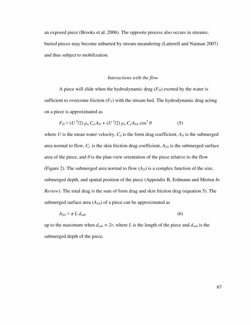
67

an exposed piece (Brooks et al. 2006). The opposite process also occurs in streams;

buried pieces may become unburied by stream meandering (Latterell and Naiman 2007)

and thus subject to mobilization.

Interactions with the flow

A piece will slide when the hydrodynamic drag (FD) exerted by the water is

sufficient to overcome friction (FF) with the stream bed. The hydrodynamic drag acting

on a piece is approximated as

FD ≈ (U 2/2) ρw Cd AN + (U

2/2) ρw Cf ASA cos3 θ (5)

where U is the mean water velocity, Cd is the form drag coefficient, AN is the submerged

area normal to flow, Cf is the skin friction drag coefficient, ASA is the submerged surface

area of the piece, and θ is the plan-view orientation of the piece relative to the flow

(Figure 2). The submerged area normal to flow (AN) is a complex function of the size,

submerged depth, and spatial position of the piece (Appendix B, Erdmann and Merten In

Review). The total drag is the sum of form drag and skin friction drag (equation 5). The

submerged surface area (ASA) of a piece can be approximated as

ASA ≈ π L dsub (6)

up to the maximum when dsub = 2r, where L is the length of the piece and dsub is the

submerged depth of the piece.

68

Figure 2. Plan view of channel with pieces of wood oriented perpendicular to the flow (θ = π/2 radians) and parallel to the flow (θ = 0 radians).

Form drag coefficients (Cd) are a function of the shape of the object, its position

in the stream, and a Reynolds number defined as

Re = 2r U/ ν (7)

where ν is the kinematic viscosity. In a simple case where the stream bed, stream banks,

and water surface are far away from the piece, they will have little effect on the drag

coefficients. For that case (approximating an infinite fluid), drag coefficients on many

different shapes of bodies have been studied extensively, and can be found in the

published literature (e.g. Hoerner 1965). Brooks et al. (2006) reviewed the literature and

selected a drag coefficient of 1.2 for wood in streams, whereas Bocchiola et al. (2006)

used dowels in flumes to obtain a drag coefficient of 1.41. Natural pieces of wood may

have greater drag due to skin friction than the smooth dowels used by Bocchiola et al.

(2006), thus we have included the skin friction component of equation (5) with a skin

friction drag coefficient Cf = 0.005 (Olson 1961).

69

The flow around a piece may also produce differences in pressure that result in a

vertical lift force. In an infinite fluid, the lift force (FL) acting on a piece can be estimated

as

FL ≈ U 2/2 Clp AN cos θ + U

2/2 Clg AN sin θ (8)

where Clp and Clg are the lift coefficients for pitch and gap lift. Pitch lift can be positive

(upwards) or negative (downwards) depending on the pitch of the piece relative to the

stream bed (γ, Figure 3); a piece with positive pitch has positive lift and a piece with

negative pitch has negative lift. Pitch lift coefficients (Clp) for objects of various shapes

are given by Hoerner (1985). The pitch lift coefficient for a cylinder is insensitive to the

fineness ratio (i.e., diameter/length, Hoerner 1985), making a javelin a suitable surrogate

for a piece of wood in terms of pitch lift. Pitch lift is greatest for pieces oriented parallel

to the direction of flow (θ = 0). For a javelin the pitch lift coefficient can be estimated as

Clp = sin2 γ cos γ (9)

Figure 3. Side view of channel illustrating pieces of wood pitched parallel to the stream bed (γ = 0 radians) and at 45° to the stream bed (γ = π/4 radians).

70

Unlike pitch lift, gap lift (Clg) is greatest for pieces oriented perpendicular to the

flow (θ = π/2), and always acts in a downward direction. Gap lift is a function of piece

diameter and the gap between the piece and the stream bed, and is caused by the

Bernoulli effect (Lei et al. 1999). When water must pass through a constricted opening

(the gap) the velocity increases and the pressure decreases; the decreased pressure under

the piece causes a downward force. Gap lift coefficients can be estimated from Lei et al.

(1999) as

Clg ≈ 0.0916 (G/2r)-0.5911 (10)

with a maximum value of Clg = 0.55.

Role of hydrology

Stream hydrology is a major determinant of wood transport. Any piece of wood

will be mobilized at a sufficient discharge, just as the largest boulders are mobilized

during extreme floods (Gordon et al. 2004). Discharge depends on hydrologic factors

including climate (mainly precipitation) and watershed characteristics such as

topography, geology, soils, vegetation, and artificial or natural storage (Gordon et al.

2004). Under uniform flow conditions, the water level and mean velocity at a channel

cross-section can be related using Manning’s equation (Olson 1961)

U = Q/Awet = n -1

R 2/3

α 1/2 (11)

where U is mean stream velocity, Q is the discharge rate, Awet is the wetted area, n is

Manning’s roughness coefficient for the channel, and R is the hydraulic radius

(approximated by the water depth in a wide channel). Manning’s roughness coefficient

71

(n) is a function of the substrate, shape, and vegetation of a channel (Arcement and

Schneider 1989). Channel roughness is also influenced by obstructions, generally rocks

and wood, which can have more direct effects on mobilization.

Interactions with obstructions

In natural streams, pieces of wood are often braced against obstructions in the

channel. Rocks, islands, or fallen trees can provide support and prevent the mobilization

of a wood piece. To become mobilized, a braced piece must rise up and over a bracing

object, requiring a net upward force. As with floatation of an unbraced piece, buoyancy

plus hydrodynamic lift must be greater than the weight of the piece, but vertical friction

(FV) must also be overcome. Vertical friction acts between a braced piece and the bracing

object and is related to the hydrodynamic drag (FD), where

FV = FD fbrace cos ψ (12)

and fbrace is the coefficient of friction of the bracing object and ψ is the angle of the

upstream face of the bracing object.

Wood pieces may also be braced against stream banks and live vegetation.

Particularly during overbank flows, a piece may become braced against trees at the edge

of the floodplain; a piece braced against trees is unlikely to be lifted over them. A piece

may also become wedged between stream banks and require a substantial force to be

mobilized. Moment forces may cause a piece to pivot off a bracing obstruction, but this

type of motion is beyond the scope of this study.

72

Theoretical predictors of wood mobilization

Based on the preceding discussion, a number of theoretical variables emerge for

predicting wood mobilization. Some relevant forces have been described above,

specifically FB, FW, FF, FD, FL, and FV. These forces can be combined into ratios that are

most likely to promote or resist mobilization. Examples are a vertical force ratio (RV,

equation 13) and a downstream force ratio (RD, equation 14)

RV = (FW + FV)/(FB + FL) (13)

RD = FF/FD (14)

The vertical force ratio (RV) thus describes the relative force acting in a downward

direction, whereas the downstream force ratio (RD) describes the relative force acting in

an upstream direction. If either ratio is < 1 then mobilization is theoretically possible, and

ratios closer to zero imply a greater likelihood of mobilization. Thus, we expect that

mobilization is most likely for pieces where the buoyancy, lift, and hydrodynamic forces

are high and the weight, vertical friction, and horizontal friction forces are low.

Additional forces that can be expected to influence wood mobilization include the

resisting force due to burial in the stream bed and the normal force exerted by bracing

objects. Neither force could be quantified under our experimental conditions; we thus

considered these forces to be either present or absent (i.e., buried/unburied,

braced/unbraced).

Aside from forces, the probability of mobilization may also be related to other

physical and positional attributes of a wood piece. These attributes make a piece more or

less likely to be in contact with the stream bed, banks, or other obstructions. We

73

identified five physical attributes likely to influence mobilization: the length ratio (L*,

ratio of piece length to the effective stream width), draft ratio (D*, ratio of piece draft to

mean depth in the channel), branching complexity, rootwad presence, and blockage (the

percentage of the wetted channel cross-sectional area occupied by the piece). We also

expected two positional attributes to influence mobilization. The lateral distance of the

wood piece from the stream bank is important because pieces in the channel are more

likely to be mobilized than those among floodplain trees, and effective depth is important

because pieces on the channel bottom are more likely to be mobilized than those

suspended above it. We next designed a field study, described below, to test our

predictions.

METHODS

Study area and streams

The study area was in forested watersheds along the north shore of Lake Superior

in Minnesota. High flows occur in area streams after spring snowmelt, but overbank

stormflows are also common in summer or fall. Nine streams with continuous discharge

data available (15-minute intervals) were selected for study (Figure 4). The study streams

were the Beaver River, French River, Knife River, Little East Knife River, Little West

Knife River, Sucker River, Talmadge Creek, Upper Knife River and West Split Rock

River. These nine streams represented a wide range of geomorphic conditions; stream

beds were dominated by cobble and gravel (Figure 5) and mean bankfull widths ranged

from 3.4 to 24.4 m.

74

A single study reach 250 to 800 m in length was established in each stream, for a

total of 4,190 m. Each study reach was divided into 10-m sections marked with wire

flags, flagging tape, and GPS. In all instances, the particular 10-m section from which

data were collected was noted. Data were collected from June to November 2007. During

the peak discharges in October 2007 wetted widths in the nine streams ranged from 3.4 to

90.7 m and mean cross-sectional water depths from 0.3 to 3.1 m.

Figure 4. Study sites (stars with arrows) along the north shore of Lake Superior in Minnesota. Duluth, Minnesota is in the southwest corner and Silver Bay, Minnesota is in the northeast corner.

75

0

50

100

150

200

250

Clay Silt Sand Gravel Cobble Boulder Bedrock

Category of dominant substrate

Nu

mb

er

of

tra

ns

ec

ts

Figure 5. Number of stream bed transects by dominant substrate for the nine streams.

Water levels in summer 2007 were low (Figure 6) due to extreme drought

conditions (USDA Drought Monitor, 8/14/07). However, storms from mid-September

through mid-October produced heavy rainfall in the study area. Rainfall observers within

10 km of Lake Superior from Duluth to Silver Bay recorded a mean of 25.3 cm of rainfall

(s.d. = 2.3) from 9/15/07 to 10/15/07, compared to 19.6 cm for the entire period from

6/15/07 to 9/15/07 (Minnesota State Climatology Office). The rainfall caused a

stormflow with a recurrence interval of 1.1 years at the only study stream with a long-

term hydrologic record (Knife River, per the St. Louis County Soil and Water

Conservation District). Although the hydrologic records were insufficient to estimate the

recurrence intervals at other study streams, the relatively uniform rainfall in the study

area suggests that the recurrence interval at other study streams was comparable to the

Knife River. Overbank flows were observed at all nine study streams during the

stormflow event.

76

Figure 6. Hydrograph for the Poplar River from June to November 2007. Hydrographs for other study streams were similar. Data from Minnesota Pollution Control Agency.

Wood data collection

In June through August of 2007, all preexisting natural pieces of wood (> 0.1 m in

diameter for a portion > 1 m in length) in the study reaches were located and marked. A

subset (n ≈ 20) of smaller pieces (> 0.05 m in diameter for a portion > 1 m in length)

were also located and marked in each study reach, for a total of 963 pieces. All pieces

that lay within the channel or that had a portion over 0.05 m in diameter extending into

the bankfull channel were assessed. Pieces were included if they were entirely dead but

still rooted, or still alive but entirely uprooted. Each piece was marked with flagging tape

and one (n=334) or three (n=629) individually numbered tags. Measurements were taken

on each piece as described below to obtain the parameters listed in Table 1. All marked

pieces in the study reaches were located again in mid-October through November 2007

after floodwaters from the early October storm had receded.

77

Total length (for the portion over 0.01 m in diameter) and diameter of each piece

were measured using a tree calipers at the ends and middle. Each piece was treated as a

cylinder for estimation of total volume, using the total length and mean diameter (i.e., the

sum of both end diameters and twice the middle diameter all divided by four). The

presence of rootwads was noted. The orientation of each piece was estimated as the

horizontal angle relative to the flow (θ, Figure 2) using categories of 0, π/6, π/3, and π/2

radians. The pitch of each piece relative to the stream bed (γ, Figure 3) was visually

estimated using categories of 0, π/6, π/4, π/3, and π/2 radians; pitch was also measured on

a subset of pieces (n = 374) using a clinometer. Pieces where a clinometer was employed

used the clinometer measurement; the remainder of the pieces used a corrected

clinometer measurement based on the relationship between visual estimates and

clinometer measurements (r2 = 0.73).

The branching complexity was assessed for each piece as described by Newbrey

et al. (2005), where higher branching complexity corresponds to a greater number of

branches and twigs. The density of each piece was also determined using a sample

obtained with an increment borer. It was noted if a piece was braced against other pieces,

live trees, rocks, or the stream channel (including pieces that had a portion above the

stream bed pinned under other pieces or rocks) or was buried. A piece of wood was

considered buried if > 5% of its cross-sectional area was embedded into the substrate or if

either end was buried in the substrate (including pieces that were entirely dead but still

rooted).

78

The location of the midpoint of each piece was noted by measuring its

longitudinal location within its 10-m section, the elevation relative to the existing water

level, and the lateral distance from the nearest bank. The elevation of the midpoint of the

piece relative to the existing water level was used in conjunction with continuous

discharge data and the hydraulics models described below to determine the absolute

elevation of each piece.

Forces acting on each piece were estimated based on characteristics of the piece

and local hydraulic conditions. The buoyancy (FB), weight (FW), and friction against the

stream bed (FF) were calculated using equations (1), (2), and (4). The hydrodynamic drag

(FD), lift force (FL), and frictional force against braces (FV) were calculated using

equations (5), (8), and (12). A bed coefficient of friction fbed = 0.2 was used, the mean of

values for sliding and rolling on gravel determined by Bocchiola et al. (2006). The

vertical coefficient of friction fbrace = 0.2 and ψ = π/2 radians were also used.

Table 1. Variables measured or calculated for each piece of wood.

Measured variables

Length > 0.1m in diameter Branching complexity Density ρlog

Total length L Bracing Orientation to flow θ

Mean diameter 2r Lateral distance from bankfull Pitch from streambed γ

Elevation Burial Rootwad presence

Calculated variables

Volume Vlog Draft D Effective depth

Weight FW Buoyancy FB Vertical force ratio RV

Submerged volume Vsub Hydrodynamic drag FD Downstream force ratio RD

Area normal to flow AN Friction force on bed FF Length ratio L*

Surface area ASA Blockage Draft ratio D*

79

Wood mobilization response data

Changes in the locations of wood pieces were determined in fall 2007; the

locations of all tagged pieces that were initially marked in summer 2007 and had

remained in each study reach were again determined in October-November. Each piece

generated a logistic data point: 0 if the piece remained within 10 m of its original

longitudinal position or 1 if it moved downstream at least 10 m. By this definition, the

response variable for mobilization addressed at the 10-m scale whether pieces initially at

rest remained at rest over the time frame of this study. Although pieces were not

remeasured, only nine pieces were known to have broken (based on the position of the

tags; the shorter portion of the piece was disregarded).

Geomorphic data

Data on stream geomorphology were collected in all study reaches in summer

2007. A survey laser and measuring tape was used to survey cross-sections every 10 m,

except at the two largest streams where 40 of 80 (Beaver River) or 12 of 50 (Knife River)

10-m sections were surveyed. Cross-sections were referenced to one another using

frequent turning points (Harrelson et al. 1994). Elevations were recorded near inflection

points along the cross-section. The bed slope was calculated for each reach as the slope

between the lowermost points at the upstream and downstream ends of the reach. The

innermost lateral location of bank vegetation > 0.02 m in stem diameter was noted on

both sides of each cross-section and used to estimate the effective stream width (Figure 7)

available to transport wood. Estimates of Manning’s roughness coefficient were made by

80

the methods of Arcement and Schneider (1989), using separate estimates for the stream

channel and floodplain of each study reach.

Figure 7. Plan view of stream channel illustrating lateral positions of trees (open circles) large enough to brace a floating piece of wood. Effective stream width was the lateral distance between the innermost trees (closed circles) for each 10-m section of stream or the actual wetted width, whichever was shorter.

Hydraulic analysis

The computer simulation model HEC-RAS 4.0 (available online)6 was used to

calculate hydraulic characteristics at each 10-m section during overbank stormflows in

fall 2007; HEC-RAS is appropriate for studying stream characteristics at a 10-m

resolution (Brooks et al. 2006). Based on the geomorphic survey data, HEC-RAS was

used to estimate unit stream power, stage, mean water velocity, and energy grade slope

(Gordon et al. 2004) at each 10-m section at the peak discharge in fall 2007. The velocity

estimates from the HEC-RAS models represent a cross-sectional average.

6 (http://www.hec.usace.army.mil/software/hec-ras/)

81

To calibrate the hydraulic model for each study reach, the initial value for channel

roughness was varied (between 0.02 and 0.07) to obtain the best fit between predicted

water stages and observed stages during summer 2007. The r2 values between predicted

and observed water stages for the summer 2007 discharges ranged from 0.77 to 1.00,

indicating good prediction of hydraulic characteristics.

Calculation of wood piece variables using hydraulic variables

The peak discharge during overbank flows in fall 2007 was used to determine the

hydraulic variables in Table 1. The effective channel width was defined as the wetted

width that was available to transport wood, taken as either the lateral distance between

the innermost trees (Figure 7) or the modeled wetted width, whichever was less. The

length ratio (L*) was calculated for each piece as the piece length divided by the effective

channel width in the initial 10-m section where the piece was located. The absolute

elevation of each piece was determined by applying the measured difference between the

piece elevation and the existing water level to the modeled stage (Figure 8). Using the

absolute elevation for each piece, the distance between the lowermost point on each piece

and the water surface (i.e., the effective depth) was determined for the fall overbank

flows. The draft ratio (D*) for each piece was calculated as the draft divided by the mean

depth in the channel in the initial 10-m section. Blockage by each piece was estimated as

AN/Awet using the original orientation and pitch of the piece. The hydrodynamic drag

acting upon each piece was calculated using equation (5). The form drag coefficient Cd

used was 1.41 (Bocchiola et al. 2006) and the skin friction drag coefficient Cf used was

82

0.005 (Olson 1961). The vertical force ratio (RV) and downstream force ratio (RD) were

calculated for each piece using equations (13) and (14). Based on the observed

distributions of RV and RD, the maximum value for RV was set to 100 and the maximum

RD was set to 10, including cases where the denominator was zero (i.e., the piece was

above the water level, Figure 8). The predictor variables did not account for flexing or

breakage of pieces, mobilization by jarring contact from other pieces or sediment in

transit, flexing or movement of bracing obstructions themselves, mobilization via rolling

or pivoting (as opposed to floatation or sliding), or human intervention.

Figure 8. Side view of stream channel illustrating a piece of wood suspended above the water surface. The measured difference between the water surface and the center of the piece was applied to the modeled stage to estimate the absolute elevation of the piece.

Data analysis

Multiple logistic regression (Weisberg 1985) was used to model the mobilization

response. Unlike multiple linear regression or discriminant function analysis, logistic

83

regression analysis does not require normally distributed response variables, nor does it

assume homogeneous variances for the response variable (Weisberg 1985). The binomial

response variable for this study (mobilization) is well-suited for logistic regression but

not for multiple linear regression. In addition, the sample size of 963 pieces provided a

suitable representation of possible cases. A multiple logistic regression model was

developed using the logistic mobilization data as the response variable. Each tagged piece

represented one data point. The predictor variables for the full model were selected to

account for known mechanisms of wood transport: vertical force ratio (RV), downstream

force ratio (RD), burial, bracing, ratio of piece length to effective channel width (length

ratio, L*), ratio of piece draft to mean depth in the channel (the draft ratio, D*), branching

complexity, rootwad presence, blockage, lateral distance from bankfull, and effective

depth of the piece. The final model was chosen using the stepAIC function of the

statistical software R (available online)7 to determine the model with the fewest

predictors that would each make a significant improvement to the AIC (Weisberg 1985).

The Variance Inflation Factor (VIF) was examined for all predictor variables in the final

model to evaluate collinearity; predictors with VIF > 2 were culled. The final model

produced a probability of mobilization for pieces under specific conditions; the goodness

of fit was evaluated using Nagelkerke’s r2 (Nagelkerke 1991) and variables were ranked

by importance according to the absolute value of their Wald Z Score.

7 (http://www.r-project.org/)

84

RESULTS

Range of variables

A total of 963 pieces of wood were tagged and measured, but some were excluded

from analyses. Two spanning logjams were present at the study reaches; wood pieces that

were in either logjam (n = 98) were omitted from analyses. Pieces in a logjam move via

congested flow (Braudrick et al. 1997), whereas this study focused on uncongested flow

where mobilization of a piece is independent of other pieces.

Wood pieces that were not in logjams (n = 865) exhibited a range of

characteristics (Table 2). For example, the mean piece length was 3.8 m with a standard

deviation (s.d.) of 3.0 m, mean diameter was 0.18 m (0.13 m), and mean wood density

was 0.75 g/cm3 (0.31 g/cm3). Many characteristics appeared to follow a chi-square

distribution (Appendix C), which is acceptable because multiple logistic regression

makes no assumptions about the distributions of predictor variables (Weisberg 1985).

85

Table 2. Mean and standard deviation for wood piece characteristics in summer 2007,

and geomorphic and hydraulic stream characteristics during peak discharges in fall 2007.

Units Mean

Buoyancy (FB) N 12 30

Weight (FW) N 13 30

Wood density (ρlog) g/cm3 0.75 0.31

Piece length (L) m 3.8 3.0

Diameter (2r) m 0.18 0.13

Volume (Vlog) m3 0.18 0.49

Pitch from stream bed (γ) rad 0.18 0.17

Effective depth m 1.06 0.76

Submerged volume (Vsub) m3 0.12 0.30

Draft (D) m 0.12 0.10

Friction on stream bed (FF) N 0.7 2.8

Piece surface area (ASA) m2 2.2 3.0

Hydrodynamic drag (FD) N 573 963

Orientation to flow direction (θ) rad 0.73 0.49

Area normal to flow (AN) m2 0.34 0.47

Lift (FL) N 0.003 0.025

Water velocity (U) m/s 1.5 0.5

Vertical force ratio (RV) - 17 49

Downstream force ratio (RD) - 1.1 3.2

Length ratio (L*) - 0.47 0.50

Draft ratio (D*) - 0.14 0.16

Branching complexity - 12 39

Blockage - 0.06 0.12

Lateral distance from bankfull m 6.7 15.6

Wetted width m 23 17

Effective stream width m 12.2 8.0

Energy grade slope m/m 0.011 0.011

Unit stream power N/m s 138 137

Mean depth in channel m 1.13 0.59

Geomorphic and hydraulic conditions also covered a wide range during peak

flows in fall 2007, whether all data were combined (Table 2) or examined by stream

(Table 3). The mean wetted width was 23 m (17 m), and the mean water depth in the

86

channels was 1.13 m (0.59 m). The mean water velocity in the channels was 1.5 m/s (0.5

m/s), and unit stream power in the channels had a mean of 138 N/m s (137 N/m s).

Table 3. Mean and standard deviation for geomorphic and hydraulic stream characteristics for each study site during peak discharges in fall 2007. Depth, velocity, and power values do not include water in the floodplain.

Stream Mean depth (m)

Water velocity (m/s)

Power (N/m s)

Bed slope (m/m)

Bankfull width (m)

Peak flow (m3/s)

Beaver River 1.66 0.30 0.86 0.32 15 35 0.001 16.0 3.0 21.7 French River 0.74 0.17 1.53 0.34 119 84 0.020 11.3 2.5 12.0

Knife River 1.51 0.29 1.44 0.22 137 57 0.006 24.4 5.3 54.7

Lt. East Knife 1.48 0.22 1.17 0.42 78 135 0.004 3.4 0.9 7

Lt. West Knife 0.53 0.15 1.15 0.33 40 36 0.012 3.7 0.8 2.1

Sucker River 0.98 0.13 1.84 0.33 252 169 0.016 9.9 2.2 17.5

Talmadge Cr. 0.78 0.14 1.62 0.25 247 135 0.025 5.3 1.6 7.0

Upper Knife 0.84 0.08 1.48 0.25 93 46 0.009 6.6 1.1 8.3

W Split Rock 2.48 0.28 1.92 0.45 153 108 0.007 6.9 0.9 54.4

Of the 865 wood pieces used in this study, 356 (41%) were mobilized during the

study period. The mean length and diameter for mobilized pieces was 2.84 and 0.15 m

whereas the mean length and diameter for stable pieces was 4.53 and 0.19 m. Mean wood

density was 0.75 and 0.76 g/cm3 for mobilized and stable pieces.

Mobilization model

The final model for mobilization was highly significant (p < 0.001) and had seven

predictor variables (Table 4). An additional variable (blockage) was present in the final

model but was culled due to a high VIF (2.656). The seven remaining predictor variables

were burial, effective depth, length ratio (L*), bracing, rootwad presence, downstream

force ratio (RD), and draft ratio (D*). Each predictor had a p-value < 0.05 and a VIF < 2,

87

indicating that the variables were not collinear. Nagelkerke’s r2 for the final model was

0.39, corresponding to a Goodman-Kruskal gamma of 0.67 and Kendall’s tau-a of 0.32.

Table 4. Variables retained in the final model for mobilization; n = 865 pieces of wood. Overall model p < 0.001 and Nagelkerke’s r2 = 0.39.

Coefficient S.E. Wald Z p-value VIF

Intercept 0.385 0.233 1.65 0.098 Burial -2.643 0.345 -7.67 <0.001 1.088

Effective depth 0.858 0.137 6.27 <0.001 1.266

Length ratio -1.517 0.261 -5.80 <0.001 1.178

Bracing -0.774 0.171 -4.54 <0.001 1.055

Rootwad presence -0.799 0.261 -3.06 0.002 1.021

Downstream force ratio -0.091 0.035 -2.59 0.010 1.115

Draft ratio -1.592 0.741 -2.15 0.032 1.183

Model sensitivity to changes in individual predictors

The probability of a positive response (i.e., mobilization) can be expressed for

individual predictors using a logistic equation as

P = exp(β0 + β1 x1)/(1 + exp(β0 + β1 x1)) (15)

where β0 was the intercept (e.g., 0.385 in Table 4), β1 was the model coefficient for the

variable of interest, x1 was the value for the variable of interest, and all other variables

were held constant. Using the model coefficient for burial (-2.643 in Table 4) equation

(15) indicated that a piece which was not buried (x1 = 0) had a 0.60 probability of being

mobilized, whereas a piece that was buried (x1 = 1) had a 0.09 probability of being

mobilized. Taking the difference (0.09 – 0.60 = -0.51) showed that a piece that was

buried was 51% less likely to be mobilized, assuming all other variables were held

constant. Similarly, a piece that was braced was 19% less likely to be mobilized than an

unbraced piece, and a piece with a rootwad was 20% less likely to be mobilized than one

88

without. Increasing the effective depth of a piece by one standard deviation from 1.06 m

(the mean value) to 1.82 m was associated with a 9% increase in the probability of

mobilization (Figure 9). Increasing the length ratio (L*) by one standard deviation from

0.47 (the mean value) to 0.97 was associated with a 17% decrease in mobilization.

Likewise, increasing the downstream force ratio or draft ratio by one standard deviation

was associated with reductions of 7% or 6%.

89

0

0.2

0.4

0.6

0.8

1

0 0.5 1 1.5 2

Effective depth

Pro

ba

bilit

y o

f m

ob

iliz

ati

on

0

0.2

0.4

0.6

0.8

1

0 0.1 0.2 0.3 0.4 0.5 0.6 0.7 0.8 0.9 1

Length ratio

Pro

ba

bilit

y o

f m

ob

iliz

ati

on

90

0

0.2

0.4

0.6

0.8

1

0 0.5 1 1.5 2 2.5 3

Downstream force ratio

Pro

ba

bilit

y o

f m

ob

iliz

ati

on

0

0.2

0.4

0.6

0.8

1

0 0.05 0.1 0.15 0.2 0.25 0.3

Draft ratio

Pro

ba

bilit

y o

f m

ob

iliz

ati

on

Figure 9. Expected probability of mobilization as a function of the effective depth, length ratio (L*), downstream force ratio (RD), or draft ratio (D*).

91

Predicting mobilization with the full model

Expanding equation (15) to consider the sensitivity of model projections the full

set of predictor variables yields

P = exp(β0 + β1 x1 + β2 x2 … + β6 x6 + β7 x7) / (16) (1 + exp(β0 + β1 x1 + β2 x2 … + β6 x6 + β7 x7)) where β1 x1 … β7 x7 correspond to coefficients and values for the seven predictor

variables. Combining the prior examples, a piece of wood that was unburied, unbraced,

and had no rootwad, effective depth of 1.82, length ratio of 0.47, downstream force ratio

of 1.1, and draft ratio of 0.14 had P = 0.71. Conversely, a piece that was buried, braced,

and had a rootwad, effective depth of 1.06, length ratio of 0.97, downstream force ratio of

4.3, and draft ratio of 0.30 had P = 0.01.

Categories for bracing

At the time of tagging in summer 2007, most pieces were not braced (n = 581,

Figure 10). Of the 284 pieces that were braced, 104 were braced by other pieces of wood,

79 were braced by live trees, 73 were braced by rocks in the channel, and 28 were braced

by the stream banks or channel itself.

92

Figure 10. Frequency of bracing of wood pieces in relation to the object on which the piece was braced in summer 2007.

DISCUSSION

Eleven variables were identified through literature review and assessed for their

potential influence on mobilization of natural pieces of wood in streams. No known study

has examined wood mobilization with such a comprehensive set of potential predictors.

Seven of the variables contributed significantly to the prediction of mobilization, as

ranked by the absolute value of their Wald Z Score: burial, effective depth, length ratio

(L*), bracing, rootwad presence, downstream force ratio (RD), and draft ratio (D*). The

overall model had a p-value < 0.001 and r2 = 0.39 (Nagelkerke 1991).

93

Our study agrees with the statement that predicting wood transport is much more

complex than sediment transport (Braudrick and Grant 2000), even with a large field

dataset and seven significant predictors. Below we discuss each of the significant

predictor variables, describe the characteristics of stable pieces, and make suggestions for

future research.

Controls of mobilization

Burial was easily most important variable in the final model for mobilization,

based on the Wald Z Score. Pieces that were partially buried were less likely to be

mobilized. Burial and unburial can remove or return a substantial amount of wood to

streams (Latterell and Naiman 2007). Although few studies have considered the effects of

burial on mobilization, when burial is included in analyses it is of primary importance

(Berg et al. 1998, Wohl and Goode 2008). Our study demonstrated the importance of

burial to mobilization using a quantitative analysis and a large number (865) of wood

pieces.

The effective depth of the wood piece was the second most important variable in

the final model for mobilization, with more-submerged pieces more likely to be

mobilized. Effective depth may function as a composite descriptor of the various

mobilizing forces acting on a piece (e.g., buoyancy, hydrodynamic drag and lift).

Effective depth also affects the likelihood that a piece will contact the stream bed before

escaping a 10-m section. In a turbulent stream, a piece floating in deep water is less likely

to contact the stream bed than the same piece floating in shallow water. Effective depth is

94

affected by stream discharge, the importance of which was recognized in the pioneering

work by Bilby (1984).

The next important variable in the final model for mobilization was the length

ratio (L*). Pieces that were long relative to the effective channel width were less likely to

be mobilized. At the 10-m scale, the length ratio may relate to the probability that a piece

becomes braced before it can escape the 10-m section. While most previous studies have

likewise found a negative relationship between length ratios and mobilization (Bilby

1984, Lienkaemper and Swanson 1987, Berg et al. 1998, Jacobsen et al. 1999, Gurnell et

al. 2002, Hassan et al. 2005, Warren and Kraft 2008), one recent study found a positive

relationship (Wohl and Goode 2008). Although the contrasting study spanned 11 years,

their definition of mobilization included breakage. It is possible that relatively longer

pieces are more prone to breakage, which could explain the discrepancy between Wohl

and Goode (2008) and other studies. Finally, we used the effective channel width to

determine our length ratio (rather than bankfull width or wetted width) to represent the

actual width available to transport wood.

Bracing was also a significant predictor of mobilization; a piece that was braced

was less likely to be mobilized. Thus, three of the variables predicting mobilization

(burial, length ratio, and bracing) are in agreement with the qualitative results of the

extensive field study by Berg et al. (1998), which did not assess the remainder of our

variables. It bears noting that, of the pieces that were braced in summer 2007, the largest

number was held by other pieces of wood, even after pieces in spanning logjams were

95

culled from the dataset. The frequency of wood pieces in a stream may provide a positive

feedback by reducing mobilization of other pieces.

Rootwad presence was associated with a lower probability of mobilization. A

rootwad presents additional surface area that may become entangled with rocks,

vegetation, or other pieces to prevent a piece from being mobilized. Rootwads tend to be

sturdy; for example if a rootwad becomes wedged between rocks it may hold the entire

piece against substantial hydrodynamic drag. Rootwads also elevate a piece, potentially

reducing the submerged volume and thus the buoyancy and hydrodynamic drag

(Braudrick and Grant 2000).

Pieces with higher downstream force ratio (RD) were less likely to be mobilized,

meaning pieces with more friction on the stream bed relative to hydrodynamic drag. The

downstream force ratio integrates the effects of piece density, volume, and submerged

volume into friction and the effects of water velocity and submerged piece area into

hydrodynamic drag. The downstream force ratio is lowest when buoyancy is greater than

weight (meaning the piece floats and has no friction with the stream bed) and the water

velocity is zero (meaning the piece is in slackwater or is above the water level). The

influence of downstream force ratio on mobilization was relatively minor after

accounting for the five preceding variables.

Draft ratio (D*) was the least important predictor variable, although the Wald Z

Score was still significant (p = 0.032). Pieces with higher draft relative to the water depth

were less likely to be mobilized. As for the length ratio, the draft ratio may affect the

probability that a piece is halted (by friction with the stream bed in this case) before it can

96

escape a 10-m section. Although prior research (Braudrick and Grant 2001, Haga et al.

2002) suggests that draft ratio may be important to entrapment, our analysis found that

draft ratio plays a relatively minor role in mobilization.

Four predictor variables were not included in the final model for mobilization: the

vertical force ratio (RV), blockage, branching complexity, and lateral distance from

bankfull. The vertical force ratio may overlap with bracing; the vertical friction for pieces

that were braced constituted 80% of total vertical forces (i.e., the sum of FB, FW, FL, and

FV) on average. The unimportance of branching complexity supports the assertion that

branches do not measurably increase the hydrodynamic drag acting on a piece (Hygelund

and Manga 2002). The value for branching complexity is also highly influenced by the

presence of small twigs (Newbrey et al. 2005), which break off easily under duress. It

bears noting, however, that the definition of mobilization used for this study (i.e., moved

at least 10 m) is conservative. Finer-scale definitions of mobilization that include any

measurable motion (Bocchiola et al. 2006) may be more sensitive but less ecologically

meaningful.

Overall, the composition of the final model indicated that mobilization under

natural conditions is a complex function of both mechanical factors (burial, length ratio,

bracing, rootwad presence, draft ratio) and hydraulic factors (effective depth, downstream

force ratio). Although our study included only a single year, the nine streams exhibited a

wide range of geomorphic and hydraulic conditions. Thus, the results from this study are

applicable to at least a similar range of conditions in other streams. Four of the final

seven predictor variables take discharge into account (i.e., effective depth, length ratio,

97

downstream force ratio, draft ratio) and the remainder have been identified as important

in other settings (Berg et al. 1998, Braudrick and Grant 2000, Wohl and Goode 2008).

Applications to stream management

The model equation (16) can be used for management of wood in streams. If a

management goal is to have stable wood, pieces can be partially buried, long relative to

the channel width, braced against other objects (e.g., stream banks, standing trees, rocks,

or larger pieces), have rootwads, and have high draft relative to the water depth. Pieces

can also have higher downstream force ratios by having higher density (increasing

weight, decreasing buoyancy, and thereby increasing friction with the stream bed) and by

being located in slow-moving water or above the waterline (thus minimizing the effective

depth).

Although pieces located above the waterline are less likely to be mobilized, they

also provide fewer ecological functions to a stream. In particular, pieces that are not

submerged do not provide stable substrate or biofilm for aquatic invertebrates, enhance

hydraulic heterogeneity, promote hyporheic recharge or transient storage, encourage pool

formation and channel meandering, or entrap leaves and other organic matter. However,

wood that is within stream channels but above the waterline can still provide overhead

cover for fish and is valuable for riparian species such as frogs, turtles, snakes, and

waterfowl.

We suggest several possibilities for improving the statistical strength of the

mobilization model. First, the resolution of hydraulic information could be increased,

98

with velocity and water level measured in the area immediately around each piece

(Bocchiola et al. 2006). Detailed hydraulic data are difficult to obtain in a field setting,

however, and the effort must be weighed against other considerations such as

investigating a broad range of conditions. Second, the amount of sturdy branches on each

piece could be measured in some other way. For example, a branching ratio could be

determined for each piece as the combined length of large branches (> 0.05 m in

diameter, excluding the main bole of the piece) divided by the length of the main bole.

Third, data could be collected to estimate the forces acting on a partially-buried piece,

using methods described by Brooks et al. (2006).

Further research is needed to better understand the processes that remove wood

from streams. For example, the process of instream decay is known to depend on the tree

species (Diez et al 2002) and water chemistry (Gulis et al. 2004) but has received

relatively little study (Hassan et al. 2005). Similarly, the processes by which wood

becomes buried and unburied in streams merit further study (Hassan et al. 2005, Latterell

and Naiman 2007). Perhaps the most important are the sociological reasons for

intentional wood removal by humans (Gregory and Davis 1993, Piegay et al. 2005,

Wyzga et al. 2009).

CONCLUSION

In this study we have collected an extensive dataset (over 800 wood pieces) to

study wood mobilization in streams. This study serves as a template for research on wood

mobilization that uses a wide range of piece characteristics and geomorphic stream

99

conditions representative of natural conditions, and uses an appropriate resolution for

hydraulic information. We have identified seven factors out of 11 tested that influence

wood mobilization in streams, and developed a model that includes all the significant

predictors. Using the relationships developed in this study, stewards of natural resources

can better manage instream wood for the benefit of stream ecosystems.

ACKNOWLEDGEMENTS

Wood and survey data were collected by Jo Fritz, Ryan Carlson, Dustin Wilman,

Nicole Rath, Levi Drevlow, Ryan Johnsen, and April Bebault. Rachael Stanze and

Nathan Schroeder collected continuous discharge data from six streams. Logistical

support was provided by Tracy Close of Minnesota Department of Natural Resources,

Marty Rye of USDA Forest Service, the Minnesota Cooperative Fish and Wildlife

Research Unit, and the Natural Resources Research Institute. Mathematical formulas in

Appendix B were derived and generously provided by Melissa Erdmann. Funding was

provided by the Minnesota Department of Natural Resources and Minnesota Sea Grant.

100

CHAPTER 4: Entrapment of wood in Minnesota streams determined by a length ratio and weight

Eric Merten8

Department of Fisheries, Wildlife and Conservation Biology

University of Minnesota

1980 Folwell Ave.

St. Paul, MN, 55108

Jacques Finlay

Department of Ecology, Evolution, and Behavior

University of Minnesota

1987 Upper Buford Circle

St. Paul, MN, 55108

Lucinda Johnson

Natural Resources Research Institute

University of Minnesota - Duluth

5013 Miller Trunk Hwy.

Duluth, MN, 55811

8 Corresponding author (e-mail: mert0042@umn.edu)

101

Raymond Newman

Department of Fisheries, Wildlife and Conservation Biology

University of Minnesota

1980 Folwell Ave.

St. Paul, MN, 55108

Heinz Stefan

Department of Civil Engineering

University of Minnesota

2 3rd

Ave. SE

Minneapolis, MN, 55455

Bruce Vondracek

USGS, Minnesota Cooperative Fish and Wildlife Research Unit9

University of Minnesota

1980 Folwell Ave.

St. Paul, MN, 55108

9 The unit is jointly sponsored by the U.S. Geological Survey, the University of Minnesota, the Minnesota Department of Natural Resources, the Wildlife Management Institute, and the U.S. Fish and Wildlife Service

102

SUMMARY

Wood deposited in streams provides a wide variety of ecosystem functions,

including enhancing habitat for key species in stream food webs, increasing geomorphic

and hydraulic heterogeneity, and retaining organic matter. Given the strong role that

wood plays in streams, factors that influence wood inputs, retention, and transport are

critical to stream ecology. Wood entrapment, the process of wood coming to rest after

being swept downstream at least 10 m, is poorly understood yet important for predicting

stream function and success of restoration efforts. Data on entrapment were collected for

a wide range of natural wood pieces (n = 344), stream geomorphology, and hydraulic

conditions in nine streams along the north shore of Lake Superior in Minnesota.

Locations of pieces were determined in summer 2007 and again following an overbank

stormflow event in fall 2007. The ratio of piece length to effective stream width (length

ratio) and the weight of the piece were determined to be of primary importance to wood

entrapment using multiple logistic regression. There are likely two reasons that both

factors were important. First, multiple measurements were made on each piece and in 419

10-m sections of stream, with a scaled resolution similar to that of flume studies. Second,

a wide natural range of piece and stream characteristics were examined. This study can

inform stream modifications to discourage entrapment at road crossings or other

infrastructure by determining the effective stream width required to pass particular wood

pieces. Conversely, these results could also be used to determine conditions that

encourage entrapment where wood is valued for ecological functions. Although the

103

regression model was highly significant, it explained only 25% of the variability in

entrapment. Entrapment remains difficult to predict in natural streams, and often may

simply occur wherever wood pieces are located when high water recedes. The process of

wood entrapment in streams merits further study, particularly under natural conditions

and by detailed methods such as used here.

INTRODUCTION AND BACKGROUND

Wood pieces deposited in streams provide a wide variety of ecosystem functions.

Foremost, wood enhances habitat conditions for key species in stream food webs,

including invertebrates and fish (Angermeier and Karr 1984, Berg et al. 1998, Johnson et

al. 2003, Eggert and Wallace 2007). Wood also increases hydraulic heterogeneity and

transient storage, promotes hyporheic recharge, encourages pool formation and channel

meandering, and retains leaves and other organic matter (Beechie and Sibley 1997, Mutz

and Rohde 2003, Mao et al. 2008, Stofleth et al. 2008). The frequency and size of wood

inputs vary in space and time (Latterell and Naiman 2007, Golladay et al. 2007) and are

strongly affected by riparian management (Flebbe and Dolloff 1995, Kreutzweiser et al.

2005, Czarnomski et al. 2008). The importance of wood for stream function is

increasingly recognized (Gregory et al. 2003), particularly as the adverse effects of

historic “woody debris” removal become more evident (Walter and Merritts 2008).

Given the strong role that wood plays in stream ecosystems, understanding the

factors that influence wood inputs and transport is critical to stream ecology and

restoration. One aspect of wood transport that is poorly understood is wood entrapment,

104

the process by which moving wood pieces in a stream come to rest after traveling

downstream for some distance. Wood entrapment is important for predicting stream

functions and success of restoration efforts; wood that is entrapped in a stream reach

enhances many local ecological functions. Thus, predicting the dynamics of wood

entrapment can be valuable for maintaining or changing the ecological function of natural

streams, and for restoring systems that have been degraded due to channel simplification,

erosion, and other human-driven changes.

Direct observation of individual pieces of wood is the optimal method for

studying wood entrapment. Other field methods rely on the examination of wood

standing stocks and assume that wood recruitment is spatially homogeneous, which is

unlikely to be true (Latterell and Naiman 2007). Studies assessing movement of

individual pieces of wood date to at least Bilby (1984), who concluded that piece length

was the primary factor in determining distance traveled before entrapment. Subsequent

field studies identified length ratios (i.e., the ratio of piece length to stream width) as

important in determining wood entrapment over a range of conditions, as reviewed by

Gurnell et al. (2002) and Hassan et al. (2005). For example, Lienkaemper and Swanson

(1987) determined that the primary factor for entrapment was the ratio of the piece length

to the channel width. Although the largest empirical study to date (n = 2,105 pieces)

found little correlation between piece length and distance traveled (r2 = 0.11, Jacobsen et

al. 1999), the lack of correlation was likely due to the use of pieces much shorter than the

width of the large river studied (Gurnell et al. 2002, Hassan et al. 2005).

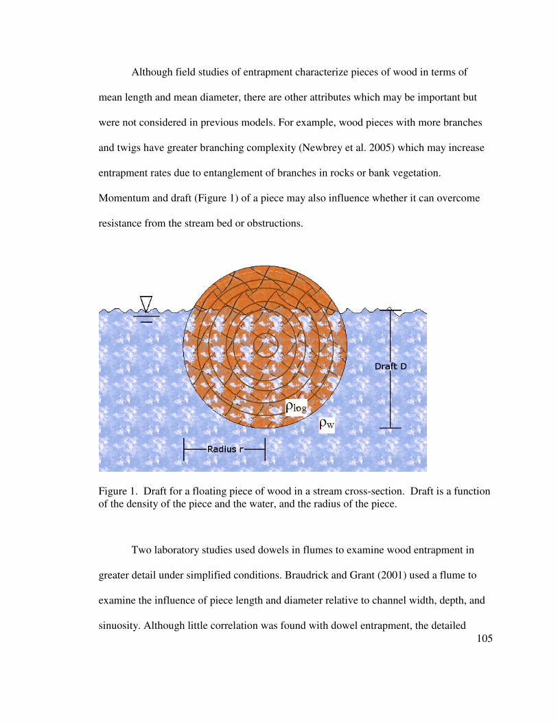
105

Although field studies of entrapment characterize pieces of wood in terms of

mean length and mean diameter, there are other attributes which may be important but

were not considered in previous models. For example, wood pieces with more branches

and twigs have greater branching complexity (Newbrey et al. 2005) which may increase

entrapment rates due to entanglement of branches in rocks or bank vegetation.

Momentum and draft (Figure 1) of a piece may also influence whether it can overcome

resistance from the stream bed or obstructions.

Figure 1. Draft for a floating piece of wood in a stream cross-section. Draft is a function of the density of the piece and the water, and the radius of the piece.

Two laboratory studies used dowels in flumes to examine wood entrapment in

greater detail under simplified conditions. Braudrick and Grant (2001) used a flume to

examine the influence of piece length and diameter relative to channel width, depth, and

sinuosity. Although little correlation was found with dowel entrapment, the detailed

106

measurements set a new standard for examinations of entrapment. Using a similar

approach with dowels in a flume, Bocchiola et al. (2006) developed robust predictions of

entrapment by floating dowels through a gauntlet of obstructions. However, it remains

unclear how well the results from flume studies can predict entrapment under the

heterogeneous conditions found in natural streams.

Studies by Haga et al. (2002) provided a starting point for integrating the detailed

mechanistic approach of flume studies with the realism of a field study. A 5.5-km reach

was divided into 24 segments, and mean water depth during peak discharges was

estimated for each segment. A total of 63 tagged pieces were placed in the stream channel

and tracked over a 13-month period; entrapment generally followed hydraulic predictions

related to the ratio of piece diameter to water depth (Haga et al. 2002). However, it is

unclear whether their results are representative of natural conditions, as all pieces studied

were cut to similar length, were shorter than the bankfull width, had branches removed,

and were similar in density.

Overall, studies of wood entrapment to date leave a number of questions

unanswered. Can the probability of entrapment be predicted for a given ratio of piece

length to channel width? Does the ratio of piece diameter to water depth proposed by

Haga et al. (2002) predict entrapment over a natural range of wood piece characteristics?

Does branching complexity or rootwad presence play a role in entrapment? The

resolution of previous field measurements may have overlooked important mechanisms,

whereas results from studies with dowels or flumes may not apply to natural wood in

natural streams.

107

Our objective in this paper is to predict and test the mechanisms controlling wood

entrapment, using a natural range of characteristics for wood pieces, stream

geomorphology, and hydraulic conditions. We integrate extensive and detailed

measurements, usually made only in flume studies, with field measurements in nine

streams. We analyze the hydraulic conditions encountered by the wood pieces in 10-m

sections by numerical modeling, and analyze the data using mechanistic approaches as

well as empirical models. We first outline the mechanisms involved with wood

entrapment to develop a theoretical basis for entrapment in streams.

MECHANISMS FOR ENTRAPMENT

A piece of wood traveling downstream may be entrapped in a variety of ways. For

example, the piece may come into contact with the stream bed and be stopped by friction,

or become lodged against an obstruction such as a boulder. Factors that can cause wood

to be entrapped in streams are described below.

Role of hydrology and hydraulics

Pieces of wood are often mobilized and entrained during peak discharge (Bilby

1984, Wohl and Goode 2008), when unit stream power, water levels, and velocities in the

channel are highest. Powerful streams have greater potential to transport wood, with unit

stream power (ω) defined as

ω = ρw gRUα (1)

108

where ρw is the density of water, g is gravity, R is the hydraulic radius for the channel

(approximated by the water depth in a wide stream), U is the stream velocity, and α is the

stream slope (Gordon et al. 2004). Under uniform flow conditions the water level and

mean velocity for a channel cross-section can be related by Manning’s equation

U = n-1

R2/3

α1/2

= Q/Awet (2)

where n is Manning’s channel roughness coefficient, Q is the discharge rate, and Awet is

the wetted cross-sectional area (Gordon et al. 2004). Channel roughness is a function of

the channel’s shape, substrate, and vegetation (Arcement and Schneider 1989). Channel

roughness is also influenced by obstructions, such as rocks, boulders, and stationary

wood pieces, which can have more direct effects on entrapment.

Interactions with the stream bed

In the simplest case, we consider an individual piece of wood traveling down a

wide stream, under conditions where interaction with the stream bed is the only

mechanism for entrapment. If no obstructions (e.g., large boulders, islands, fallen trees)

are present, the piece may stop when it encounters a shallow stream reach and contacts

the stream bed. If the shallow area is extensive, it may exert sufficient friction to reduce

or stop the piece’s forward momentum and cause the wood to be entrapped. The

momentum (M) of a wood piece is defined as

M = m U (3)

109

where m is the mass of the piece (i.e., density multiplied by volume). Piece velocity (U)

is approximately equal to water velocity for a floating piece that is not in contact with the

stream channel (Braudrick and Grant 2001).

The draft (D, Figure 1) is the primary variable that controls whether a wood piece

will contact the stream bed. Draft refers to the submerged depth of a floating piece, and

can be estimated from Braudrick and Grant (1997) from piece radius and density as

D = 2r (0.05 + 0.9 (ρlog /ρw)) (4)

where r is the radius of the piece and ρlog is the density of the piece. A piece contacts the

stream bed when the draft exceeds the water depth; the ratio of piece draft to the water

depth (draft ratio) is therefore an indicator of entrapment potential. Water depth can be

quite variable in natural streams (Gordon et al. 2004) even when obstructions are not

present; overall conditions can be summarized using the mean depth in the channel.

The blockage may also affect the probability that a wood piece will make contact

with the stream bed or banks. Blockage is the proportion of the wetted area occupied by

the piece. Blockage is heavily influenced by the orientation of the piece; blockage is least

for pieces oriented parallel to the direction of flow and greatest for those oriented

perpendicular to the flow. Pieces tend to orient themselves parallel to flow once

mobilized (Braudrick and Grant 2001). The orientation of a piece also affects the

probability that it will encounter shallow areas; a piece oriented perpendicular to the

direction of flow is more likely to encounter shallow areas than a piece oriented parallel

to the flow.

110

Interactions with obstructions in the stream channel

In natural streams, stationary obstructions are often present, such as large

boulders, islands, and other pieces of wood. The process of entrapment by obstructions is

determined by several contingencies. First, a piece must encounter an obstruction. The

probability of encounter is a function of the density of obstructions present (Bocchiola et

al. 2006), the draft of the piece relative to the elevation of the obstruction, and the

orientation of the piece (with pieces oriented parallel to the flow least likely to encounter

obstructions). Second, the obstruction must be sufficiently anchored to resist the forces

exerted by the impact of a moving wood piece. If the obstruction is a smaller piece of

wood, for example, it may become dislodged and the original piece may escape

entrapment. Third, the piece must not pivot off the obstruction. The moment forces that

determine whether a piece will pivot are a function of the location along the piece that

encounters the obstruction; pieces that contact an obstruction at their midsection are less

likely to pivot than pieces that encounter an obstruction near either end.

A wood piece may also encounter a group of obstructions. If a piece becomes at

once braced against multiple obstructions, the chance of dislodging the obstructions is

diminished. For example, the aggregate resisting force exerted by several small rocks

may be sufficient to entrap a large floating piece, even if the piece would have dislodged

any one of the rocks in isolation. A group of obstructions may also reduce the probability

that a piece will pivot and continue downstream; a piece that bridges multiple

obstructions affords less hydraulic leverage.

111

Interactions with stream banks and vegetation

Stream banks can entrap pieces of wood via two mechanisms. First, long pieces

may become wedged across the stream channel. The primary factor in determining the

distance a piece travels (which depends on the probability of entrapment) is the ratio of

the piece length to the bankfull channel width (Lienkaemper and Swanson 1987, Gurnell

et al. 2002, Hassan et al. 2005). We define a ratio of piece length to stream width as a

length ratio. Second, a wood piece may become entrapped against the stream banks in

sinuous streams. Braudrick and Grant (2001) predicted that pieces would become

entrapped on the outside of meander bends, as measured by the radius of curvature for the

stream. The forward momentum of a piece may carry it against the outside bank when the

meander bend has a small radius of curvature, providing an opportunity for the piece to

be entrapped by the bank.

Bank vegetation can also be important to entrapment (Jacobsen et al. 1999,

Millington and Sear 2007, Opperman and Merenlender 2007). During high discharge,

pieces may become entangled in live vegetation and held fast if the vegetation has

sufficient structural strength. Riparian vegetation can thus reduce the wetted stream width

that is effectively available to transport wood.

Predictors for wood entrapment

Based on the preceding discussion, we assembled seven variables as potential

predictors for entrapment of wood pieces in natural streams. We considered six variables

as likely to affect the probability that a piece would contact the stream bed, banks, or

112

other obstructions: piece weight, draft ratio, length ratio, branching complexity, rootwad

presence, and blockage. We considered an additional variable (momentum) as likely to

affect the probability that a piece is pushed past an obstruction after an encounter.

Previous studies have shown length ratio or draft ratio as important and have either not

detected or not examined a contribution from weight, branching complexity, rootwad

presence, blockage, and momentum. To test the relation of our seven variables to

entrapment, we designed a field study in northern Minnesota that encompassed a wide

range of conditions found in temperate forested streams.

FIELD DATA COLLECTION

Study design

We examined the mechanisms of wood entrapment in nine streams of forested

watersheds along the north shore of Lake Superior in Minnesota (Figure 2). The streams

had continuous discharge data available; a study reach was established in each stream

near the discharge gage. The study reach at each stream was 250 to 800 m in length

(4,190 m total) and was divided into 10-m sections (marked with wire flags, flagging

tape, and GPS) as the basis for piece locations and geomorphic conditions. Stream beds

were dominated by cobble and gravel (Figure 3), and mean bankfull widths of the nine

study reaches ranged from 3.4 to 24.4 m.

Water levels in summer 2007 were low (Figure 4) due to extreme drought

conditions (USDA Drought Monitor, 8/14/07). However, storms from mid-September

through mid-October produced heavy rainfall in the study area; rainfall observers within

113

10 km of Lake Superior from Duluth to Silver Bay recorded an average of 25.3 cm of

rainfall (s.d. = 2.3) from 9/15/07 to 10/15/07, compared to 19.6 cm for the entire period

from 6/15/07 to 9/15/07 (Minnesota State Climatology Office). The rainfall caused a

stormflow with a recurrence interval of 1.1 years at the only study stream with a long-

term hydrologic record (Knife River, per the St. Louis County Soil and Water

Conservation District). Although the hydrologic records were insufficient to estimate the

recurrence intervals at other study streams, the relatively even rainfall throughout the

study area (i.e., 25.3 cm with s.d. of 2.3) suggests that the recurrence interval at other

study streams was comparable to the Knife River. Overbank discharges were observed at

all nine study streams during the stormflow event.

Figure 2. Study sites (stars with arrows) along the north shore of Lake Superior in Minnesota. The three northernmost sites were not sampled in fall 2007. Duluth, Minnesota is in the southwest corner and the Canadian border is in the northeast corner.

114

0

50

100

150

200

250

Clay Silt Sand Gravel Cobble Boulder Bedrock

Category of dominant substrate

Nu

mb

er

of

tra

ns

ec

ts

Figure 3. Number of stream bed transects by dominant substrate, for the nine streams combined.

Figure 4. Hydrograph for the Poplar River during the study period from June to November 2007. Hydrographs at other study streams were similar. Data from Minnesota Pollution Control Agency.

115

Wood data

In June through August of 2007, all preexisting wood pieces (> 0.1 m in diameter

for a portion > 1 m in length) in the study reaches were located and marked. A subset (n ≈

20) of smaller pieces (> 0.05 m in diameter for a portion > 1m in length) were also

located and marked in each study reach, for a total of 956 pieces. Pieces were included if

they were entirely dead but still rooted, or still alive but entirely uprooted. Measurements

were taken on each piece as described below to obtain the parameters listed in Table 1.

All pieces that lay within the channel or that had a portion > 0.05 m in diameter

extending into the bankfull channel were included. Each piece was marked twice with

flagging tape and one (n=334) or three (n=629) individually numbered tags. Total length

(for the portion > 0.01 m in diameter) and mean diameter were measured using a tree

calipers at both ends and the middle of each piece. Rootwads were noted if present. All

marked pieces in the study areas were located again in mid-October through November

2007 (after floodwaters had receded), including pieces that had been ejected onto the

floodplain. Branching complexity was assessed for each piece following Newbrey et al.

(2005), and density was determined using a sample obtained with an increment borer.

Weight of each piece was estimated as the product of volume and density, and draft of

each piece was estimated using the density and mean radius per equation (4).

116

Table 1. Variables measured or calculated, see text for details.

Measured by piece Measured by 10-m section

Total length Cross-sectional elevations

Diameter (2r) Stream gradient (slope)

Wood density (ρlog) Effective stream width

Branching complexity

Rootwad presence

Calculated by piece Calculated by 10-m section

Volume (Vlog) Mean velocity in channel (U)

Weight Mean channel depth

Draft (D) Unit stream power in channel (ω)

Length ratio (L*) Wetted area in channel

Draft ratio (D*)

Momentum (M)

Blockage

Entrapment was examined further with a new cohort of pieces in 2008. All new

(i.e., unmarked) pieces that were > 0.1 m in diameter for a portion > 1 m in length were

located in June through August 2008 in each study reach. Three additional study reaches

were sampled where all pieces had been marked in summer 2007 but not revisited in fall

2007, while one reach sampled in fall 2007 was not revisited in summer 2008. Pieces that

were clearly recruited locally from riparian trees within the study reach (n = 22 freshly

fallen trees) were excluded in 2008; all other new pieces (n = 178) were assumed to have

moved from upstream of the reach. The method of entrapment was noted for each new

piece using the following categories: lying loose in the channel, braced by rocks, braced

by other pieces of wood, braced by the stream banks or bed, braced by live trees but with

117

the center of the piece remaining within 1 m of the bankfull channel, or ejected onto the

floodplain with the center > 1 m outside the bankfull channel.

Stream geomorphic data

Data on stream geomorphology were collected for all study reaches in summer

2007. Cross-sections were surveyed every 10 m in each study reach using a measuring

tape and a laser level on a tripod (Harrelson et al. 1994), except at the two largest streams

where 40 of 80 (Beaver River) or 12 of 50 (Knife River) 10-m sections were surveyed.

The bed slope was calculated for each reach using the difference in elevation between the

lowermost points at the upstream and downstream ends of the reach. The effective stream

width was estimated for each 10-m section as the shortest unobstructed width for flows

0.5 m above bankfull (Figure 5). Vegetation was considered to be obstructive if it was at

least 0.02 m in stem diameter. Initial estimates of Manning’s roughness coefficient for

the channel and the floodplain were made using the methods of Arcement and Schneider

(1989).

118

Figure 5. Plan view of channel illustrating lateral positions of trees (open circles) large enough to brace a floating piece of wood. Effective stream width was defined as the lateral distance between the innermost trees (closed circles) for each 10-m section of stream or the actual wetted width, whichever was shorter.

Hydraulic data

The computer simulation model HEC-RAS 4.0 (available online)10 was used to

calculate hydraulic parameters for each 10-m section; HEC-RAS is appropriate for

studying stream characteristics at the 10-m resolution (Brooks et al. 2006). Based on

geomorphic survey data, HEC-RAS was used to estimate unit stream power, stage,

velocity, and energy grade slope (Gordon et al. 2004) at each 10-m section for discharges

corresponding to the peak flow during overbank conditions in fall 2007. Although

overbank flows were included in the models and used for wetted width, only the portion

of the discharge that was in the bankfull channel was considered when calculating mean

velocity, depth, unit stream power, and wetted area (Table 1).

To calibrate the hydraulic model for each study reach, the initial estimate for

Manning’s channel roughness coefficient was varied (between 0.02 and 0.07) to obtain

the best fit between the predicted and observed stream stage as measured at each cross-

10 (http://www.hec.usace.army.mil/software/hec-ras/)

119

section during summer 2007. The final r2 values between the predicted and observed

stream stages ranged from 0.77 to 1.00.

Wood entrapment

In fall 2007, after floodwaters had receded, we located tagged wood pieces in

each study reach. Pieces that traveled downstream at least 10 m were used; pieces that did

not move or that moved less than 10 m were not classified as mobilized and were thus

culled from the dataset. The dataset of pieces that moved at least 10 m was split into two

groups: those that left the study reach and were not found and those that traveled

downstream but were entrapped before leaving the study reach. We used a logistic

response for subsequent analyses of entrapment; pieces in the former group were

assigned a 0 and pieces in the latter group were assigned a 1. Although pieces were not

remeasured, only seven mobilized pieces were known to have broken (based on the

position of the tags; the shorter portion of the piece was disregarded). For each piece that

left the study reach, we recorded the specific 10-m sections the piece passed through, and

associated the mean geomorphic and hydraulic data of those sections with that piece. For

each piece that moved but was entrapped within the study reach we used the geomorphic

and hydraulic data of the section in which the piece was entrapped.

DATA ANALYSIS METHODS

Data from wood pieces, stream geomorphology, and hydraulic simulations were

used to quantify predictor variables considered likely to influence wood entrapment. The

120

length ratio was piece length divided by effective stream width, and the draft ratio was

piece draft divided by mean depth in the channel. Blockage was calculated as the

submerged area (assuming the piece was oriented parallel to flow as suggested by

Braudrick and Grant 2001) divided by the wetted channel area. Weight of each piece was

its volume multiplied by density, and momentum of each piece was calculated using

equation (3) assuming the piece traveled at the same velocity as the flow (Braudrick and

Grant 2001).

A multiple logistic regression model was developed to determine the factors most

important to wood entrapment, using the logistic entrapment data as the response

variable. The predictor variables for the initial model were length ratio, weight, draft

ratio, branching complexity, rootwad presence, blockage, and momentum. The final

model was chosen using the statistical software R (available online)11 to examine the best

fit between possible combinations of predictor variables and the logistic response

variable. The final model had the lowest AIC among all models with Variance Inflation

Factor < 2 for all predictor variables (to avoid collinearity). The regression equation for

the final model produced a probability of entrapment for a given piece passing through a

given 10-m section.

RESULTS

A total of 956 pieces of wood were tagged and measured, but most were excluded

from analyses for several reasons. First, pieces (n=98) were excluded if they were

11 (http://www.r-project.org/)

121

initially part of a spanning logjam. These pieces would be expected to exhibit congested

flow, where all pieces in the logjam would travel downstream en masse rather than

independently from one another (Braudrick et al. 1997). Two spanning logjams were

initially present; both were completely mobilized by the high discharge in fall 2007 and

likely did not influence entrapment of other pieces. Second, an additional 12 pieces were

excluded because they became entrapped by a culvert at the downstream end of a study

reach. Entrapment by culverts was only observed at one of the study reaches, where two

6-m culverts had been placed side by side for a road crossing. Third, pieces (n = 502)

were excluded if they traveled less than 10 m between summer and late fall 2007, thus

there were a total of 344 wood pieces for analysis of entrapment.

Wood pieces and streams covered a range of characteristics (Table 2). For

example, the mean piece length was 2.8 m with a standard deviation (s.d.) of 2.1 m, mean

diameter was 0.15 m (0.13 m), and mean wood density was 0.74 g/cm3 (0.33 g/cm3). The

mean wetted width of the streams was 24 m (15 m), and mean water depth in the channels

was 1.3 m (0.6 m). The mean water velocity in the channels was 1.4 m/s (0.6 m/s), and

unit stream power in the channels had a mean of 125 N/m s (113 N/m s). Many

characteristics appeared to follow a chi-square distribution (Appendix D), which is

acceptable because multiple logistic regression is not constrained by the distributions of

predictor variables (Weisberg 1985). The study streams varied within and among

themselves in geomorphic and hydraulic characteristics (Table 3).

122

Table 2. Mean and standard deviation for characteristics of wood pieces and 10-m stream

sections at the nine study reaches.

Units Mean

Piece length m 2.8 2.1 Length ratio - 0.31 0.36

Diameter (2r) m 0.15 0.13

Wood density (ρlog) g/cm3 0.74 0.33

Draft (D) m 0.1 0.09

Draft ratio - 0.09 0.11

Branching complexity - 6 22

Volume (Vlog) m3 0.11 0.5

Blockage - 0.01 0.02

Weight N 8 27

Vertical force ratio - 1.1 0.2

Momentum kg m/s 10 29

Wetted width m 24 15

Mean depth in channel m 1.3 0.6

Water velocity (U) m/s 1.4 0.4

Unit stream power (ω) N/m s 125 113

Energy grade slope m/m 0.008 0.009

Effective stream width m 13.4 7.6

Table 3. Mean and standard deviation for hydraulic and geomorphic characteristics for each study site during peak discharges in fall 2007. Depth, velocity, and power values do not include water in the floodplain.

Mean wetted depth (m)

Water velocity (m/s)

Power (N/m s)

Bed slope (m/m)

Bankfull width (m)

Peak discharge (m3/s)

Beaver River 1.66 0.30 0.86 0.32 15 35 0.001 16.0 3.0 21.7 French River 0.74 0.17 1.53 0.34 119 84 0.020 11.3 2.5 12.0

Knife River 1.51 0.29 1.44 0.22 137 57 0.006 24.4 5.3 54.7

Lt. East Knife 1.48 0.22 1.17 0.42 78 135 0.004 3.4 0.9 7

Lt. West Knife 0.53 0.15 1.15 0.33 40 36 0.012 3.7 0.8 2.1

Sucker River 0.98 0.13 1.84 0.33 252 169 0.016 9.9 2.2 17.5

Talmadge Cr. 0.78 0.14 1.62 0.25 247 135 0.025 5.3 1.6 7.0

Upper Knife 0.84 0.08 1.48 0.25 93 46 0.009 6.6 1.1 8.3

W Split Rock 2.48 0.28 1.92 0.45 153 108 0.007 6.9 0.9 54.4

*Brule River 2.27 0.61 2.20 0.61 515 439 0.012 22.2 3.3 104.0

*East Beaver 1.20 0.26 1.14 0.35 91 76 0.008 11.7 3.2 16.3

*Poplar River 1.82 0.33 3.07 0.55 1111 432 0.034 10.9 2.4 62.3

*2008 bracing study only

123

Of the 344 wood pieces that met the criteria for this study, 110 (32%) were

entrapped before leaving the study reach; the mean length and diameter for entrapped

pieces was 3.42 and 0.19 m whereas the mean length and diameter for non-entrapped

pieces was 2.51 and 0.13 m. Mean wood density was 0.81 and 0.71 g/cm3 for entrapped

and non-entrapped pieces.

The final model for entrapment was highly significant (p < 0.001) and included

four predictor variables (Table 4). Nagelkerke’s r2 for the final model was 0.25,

corresponding to a Goodman-Kruskal gamma of 0.50 and Kendall’s tau-a of 0.22. The

four predictor variables were the length ratio, weight, branching complexity, and rootwad

presence. However, branching complexity and rootwad presence contributed little to the

model. The individual p-values for branching complexity and rootwad presence were >

0.05, and rootwad presence would have been excluded from the final model if the AIC

penalty were increased from 2 to 3.

Table 4. Variables retained in the final model for entrapment; n = 344 pieces of wood. Overall model p < 0.001 and Nagelkerke’s r2 = 0.25.

Coefficient S.E. Wald Z p-value VIF

Intercept -1.783 0.214 -8.34 <0.001 Length ratio 2.959 0.618 4.79 <0.001 1.205

Weight 0.044 0.018 2.41 0.0158 1.169

Br Complexity -0.011 0.007 -1.72 0.0846 1.230

Rootwad -0.805 0.573 -1.41 0.1599 1.034

Using the multiple logistic regression results, the probability (P) of entrapment

was calculated for each predictor as

124

P = exp(β0 + β1 x1)/(1 + exp(β0 + β1 x1)) (5)

where β0 was the intercept (e.g., -1.783 in Table 4), β1 was the model coefficient for the

variable of interest, and x1 was the value for the variable of interest, with all other

variables held constant. Using the model coefficient for the length ratio (2.959 in Table

5), equation (5) indicated that a piece with the mean length ratio (x1 = 0.31) had a 0.30

probability of being entrapped, whereas an increase to one standard deviation above the

mean ((x1 = 0.67) was associated with a 0.55 probability of entrapment. Taking the

difference (0.55 – 0.30 = 0.25) indicated that a piece with the higher length ratio was

25% more likely to be entrapped, assuming all other variables were held constant.

Similarly, increasing the weight of a piece from the mean value (8) to one standard

deviation above the mean (35) was associated with a 15% increase in the probability of

entrapment (Figure 6). Branching complexity and rootwad presence had weaker effects

on entrapment. Decreasing the branching complexity from 6 (the mean value) to 1 (no

branches, the least value) was associated with a 1% increase in the probability of

entrapment, and the probability of entrapment was 7% lower if a rootwad was present.

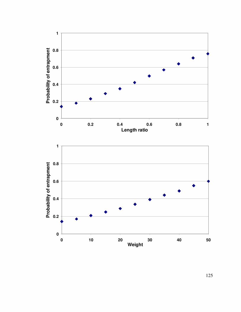
125

0

0.2

0.4

0.6

0.8

1

0 0.2 0.4 0.6 0.8 1

Length ratio

Pro

ba

bilit

y o

f e

ntr

ap

me

nt

0

0.2

0.4

0.6

0.8

1

0 10 20 30 40 50

Weight

Pro

ba

bilit

y o

f e

ntr

ap

me

nt

126

0

0.2

0.4

0.6

0.8

1

0 5 10 15 20 25 30 35 40 45 50

Branching complexity

Pro

ba

bilit

y o

f e

ntr

ap

me

nt

Figure 6. Expected probability of entrapment as a function of the length ratio, weight, or branching complexity.

Expanding equation (5) to consider changes in the full set of predictor variables

yields

P = exp(β0 + β1 x1 + β2 x2 + β3 x3 + β4 x4) / (6) (1 + exp(β0 + β1 x1 + β2 x2 + β3 x3 + β4 x4)) where β1 x1 … β4 x4 correspond to coefficients and values for the four predictor variables.

Combining the prior examples, a piece of wood with length ratio of 0.31, weight of 8,

branching complexity of 6, and a rootwad had a probability of entrapment P = 0.20.

Conversely, a piece with length ratio of 0.67, weight of 35, branching complexity of 1,

and no rootwad had P = 0.85.

127

A total of 166 new pieces were entrapped in 2008 (Figure 7). The most common

method of entrapment was pieces that were lying loose in the channel (n = 72), followed

by pieces that were braced by other pieces of wood in the channel (n = 48), ejected onto

the floodplain (n = 18), braced by rocks in the channel (n = 14), braced by the stream

banks or bed (n = 9), and braced by live vegetation in the channel (n = 5, mainly trees).

0

20

40

60

80

Loose in

channel

Braced by

wood

On floodplain Braced by

rocks

Braced by

banks/bed

Braced by

vegetation

Nu

mb

er

of

pie

ce

s

Figure 7. Numbers of new pieces found in 2008 in three stream reaches, according to location or manner in which pieces were braced.

DISCUSSION

We found two factors to be of primary importance for wood entrapment in natural

streams: the ratio of piece length to effective stream width (length ratio) and piece

weight. The coefficient of determination for the entrapment model, while not high (i.e.,

128

0.25), was substantially stronger than obtained in some studies (e.g., 0.01 by Jacobsen et

al. 1999 and 0.06 by Braudrick and Grant 2001). The reason may be that we evaluated a

diverse set of conditions. Our study included a natural range of wood pieces,

geomorphology, and hydraulics from nine streams, providing the entrapment model with

much variability to explain. Although a higher coefficient of determination was obtained

using a dense network of obstructions in a flume (Bocchiola et al. 2006), the applicability

of those results to natural conditions is unclear.

Pieces with higher length ratios were more likely to be entrapped, according to

our multiple logistic regression model. Previous studies have also determined that the

ratio of piece length to stream width was of primary importance for entrapment

(Lienkaemper and Swanson 1987, Gurnell et al. 2002, Hassan et al. 2005, Wyzga and

Zawiejska 2005). However, those studies used bankfull channel width as the measure of

stream width rather than effective stream width, which takes into account both the actual

wetted width and the infringement of woody vegetation.

Weight was also important in the final model for entrapment; heavier pieces were

more likely to be entrapped. Piece weight is the product of volume and density, which

both suggest possible explanations for the positive association of weight with entrapment.

Greater volume may increase the probability that a piece will contact obstructions,

including submerged obstructions as discussed previously (e.g., large boulders, islands,

or other pieces of wood) or above-water obstructions such as tree roots and low-hanging

branches. Higher piece density increases draft, and thus the likelihood that the piece will

contact the stream bed. Weight may therefore relate to the same mechanisms as draft

129

ratio and blockage (i.e., entrapment from contact with obstructions or the stream bed) and

is itself a component of momentum.

Branching complexity and rootwad presence were also included in the final model

for entrapment. Contrary to our predictions, pieces with higher branching complexity and

rootwads were less likely to be entrapped. An unknown mechanism may be at work with

branching complexity and rootwad presence, or the variables may be correlated with

some unmeasured parameter that decreased the likelihood of entrapment. However, the

statistical significance of both variables was weak (the individual p-values for both

variables were > 0.05) and the predictors may not be meaningful. Branching complexity

is influenced by the number of small twigs (Newbrey et al. 2005), which are unlikely to

play a role in entrapment. A small twig could break off if, for example, it became caught

between rocks but was unable to resist the hydrodynamic drag acting on the full piece.

Future studies might instead consider a branching ratio, such as the combined length of

large branches (> 0.05 m in diameter, excluding the main bole of the piece) divided by

the length of the main bole.

The final model did not include draft ratio, momentum, or blockage; those

variables had no significant influence on entrapment after accounting for length ratio,

weight, branching complexity, and rootwad presence. Although previous studies have

suggested that draft ratio influences entrapment (Braudrick and Grant 2001, Haga et al.

2002), those studies minimized the influence of the length ratio by using pieces that were

shorter than the channel width. Our dataset was much more diverse in terms of length

130

ratio, piece weight, branching complexity, and rootwad presence (Braudrick and Grant

2001, Haga et al. 2002) and covered a natural range of conditions.

The final model equation (6) can be applied to a range of conditions, as outlined

in Table 3. Although the current study included only a single year, the study streams

exhibited a range of geomorphic and hydraulic conditions, thus the final model is likely

applicable to at least a similar range of conditions in other streams. The peak discharges

for the study period varied from 2.1 to 54.7 m3/s at the nine study streams, corresponding

to a range of mean wetted widths from 3.8 to 71.2 m. Lengths of pieces were from 1.0 to

15.3 m with estimated weights from 0.08 to 327 N. Our analyses are thus applicable to

natural pieces and streams that are of interest to stream managers.

Our study can enhance management of wood in streams. For example, the model

equation (6) could be used to determine the effective stream width required to reduce

wood entrapment around road crossings or other infrastructure, provided that data were

collected on wood characteristics. The requisite stream width, in particular, could be used

to design bridge spans or culvert diameters. It bears noting that the pair of culverts in one

study reach entrapped a disproportionate number of pieces, including 42 marked pieces

(that were excluded from analyses). Using a mean piece length of 2.8 m, our model

equation associates a 33% reduction in entrapment with replacing a 3-m culvert with a 6-

m span bridge.

Alternatively, our study may also be applied to promote wood entrapment in

managed or restored streams where wood is valued for its ecological functions. The

model equation (6) can be used to determine the effective stream width required to entrap

131

pieces of a given length. Alternatively, the model can be used for a given stream width to

determine the length of pieces required to become entrapped. If natural wood pieces of

the required size are not available, short-term wood additions and long-term riparian

management may be used to increase present and future standing stocks of instream

wood (Murphy and Koski 1989, Czarnomski et al. 2008).

Regardless of input levels, entrapment of wood in streams begets more wood in

streams (Abbe and Montgomery 2003, Bocchiola et al. 2008, Warren and Kraft 2008). Of

the new pieces of wood that were entrapped in 2008, more pieces were entrapped by

other pieces of wood than were ejected onto the floodplain or entrapped by rocks, stream

banks, or vegetation. No spanning logjams were present in 2008; scattered pieces of

wood provide valuable ecological functions and a positive feedback toward further wood

accumulation even without the influence of spanning logjams.

CONCLUSION

Entrapment remains difficult to predict in natural streams. Although the model

derived in this study explained more variability in entrapment than previous field studies,

the coefficient of determination was only 0.25. Of the new pieces entrapped in 2008, a

full 43% were lying loose in the channel and not entrapped by any obvious mechanism.

In some cases, entrapment may simply occur wherever the piece is located when high

water recedes (Jacobsen et al. 1999), and be unrelated to characteristics of the piece or

the stream channel. The process of wood entrapment in streams merits further study for

predicting wood’s ecological functions and the success of restoration efforts.

132

ACKNOWLEDGEMENTS

Wood and survey data were collected by Jo Fritz, Ryan Carlson, Dustin Wilman,

Nicole Rath, Levi Drevlow, Ryan Johnsen, and April Bebault. Rachael Stanze and

Nathan Schroeder collected continuous discharge data from six streams. Logistical

support was provided by Tracy Close of Minnesota Department of Natural Resources,

Marty Rye of USDA Forest Service, the Minnesota Cooperative Fish and Wildlife

Research Unit, and the Natural Resources Research Institute. Funding was provided by

the Minnesota Department of Natural Resources and Minnesota Sea Grant.

133

BIBLIOGRAPHY

Abbe, T.B. and D.R. Montgomery. 2003. Patterns and processes of wood debris

accumulation in the Queets river basin, Washington. Geomorphology 51:81-107.

Aiken L. and S. West. 1991. Multiple regression: testing and interpreting interactions.

Sage Publications, Newbury Park, CA.

Alexander G.R. and E.A. Hansen. 1986. Sand bed load in a brook trout stream. North

American Journal of Fisheries Management 6:9-23.

Angermeier, P.L. and J.R. Karr. 1984. Relationships between woody debris and fish

habitat in a small warmwater stream. Transactions of the American Fisheries

Society 113:716-726.

Arcement, G.J. and V.R. Schneider. 1989. Guide for selecting Manning's roughness

coefficients for natural channels and flood plains. U.S. Geological Survey Water-

Supply Paper 2339.

Austin J. and S. Colman. 2008. A century of temperature variability in Lake Superior.

Limnology and Oceanography 53:2724-2730.

134

Baltz D.M., P.B. Moyle, and N.J. Knight. 1982. Competitive interactions between

benthic stream fishes, riffle sculpin Cottus gulosus, and speckled dace

Rhinichthyes osculus. Canadian Journal of Fisheries and Aquatic Sciences

39:1502-1511.

Beechie, T.J. and T.H. Sibley. 1997. Relationships between channel characteristics,

woody debris, and fish habitat in northwestern Washington streams. Transactions

of the American Fisheries Society 126:217-229.

Berg, N., A. Carlson, and D. Azuma. 1998. Function and dynamics of woody debris in

stream reaches in the central Sierra Nevada, California. Canadian Journal of

Fisheries and Aquatic Sciences 55:1807-1820.

Beschta R.L., R.E. Bilby, G.W. Brown, L.B. Holby, and T.D. Hofstra. 1987. Stream

temperature and aquatic habitat: fisheries and forestry interactions. In: Salo, E.O.

and T.W. Cundy, Streamside Management: Forestry-Fishery Interactions, pp.

191-232. Institute of Forest Resources, University of Washington, Seattle,

Washington.

Bilby, R.E. 1984. Removal of woody debris may affect stream channel stability. Journal

of Forestry 82:609-613.

135

Bocchiola, D., M.C. Rulli, and R. Rosso. 2006. Transport of large woody debris in the

presence of obstacles. Geomorphology 76:166-178.

Bocchiola, D., M.C. Rulli, and R. Rosso. 2008. A flume experiment on the formation of

wood jams in rivers. Water Resources Research 44:1-17.

Bojsen B.H. and R. Barriga. 2002. Effects of deforestation on fish community structure in

Ecuadorian Amazon streams. Freshwater Biology 47:2246-2260.

Borg D., I. Rutherford, and M. Stewardson. 2007. The geomorphic and ecological

effectiveness of habitat rehabilitation works: continuous measurement of scour

and fill around large logs in sand-bed streams. Geomorphology 89:205-216.

Boughton D.A., M. Gibson, R. Yedor, and E. Kelley. 2007. Stream temperature and the

potential growth and survival of juvenile Oncorhynchus mykiss in a southern

California creek. Freshwater Biology 52:1353-1364.

Braudrick, C.A., G.E. Grant, Y. Ishikawa, and H. Ikeda. 1997. Dynamics of wood

transport in streams: a flume experiment. Earth Surface Processes and Landforms

22:669-683.

136

Braudrick, C.A. and G.E. Grant. 2000. When do logs move in rivers? Water Resources

Research 36:571-583.

Braudrick, C.A. and G.E. Grant. 2001. Transport and deposition of large woody debris in

streams: a flume experiment. Geomorphology 41:263-283.

Broadmeadow, S. and T.R. Nisbet. 2004. The effects of riparian forest management on

the freshwater environment: a literature review of best management practice.

Hydrology and Earth System Sciences 8:286-305.

Brooks, A.P., T. Abbe, T. Cohen, N. Marsh, S. Mika, A. Boulton, T. Broderick, D. Borg,

and I. Rutherfurd. 2006. Design guidelines for the reintroduction of wood into

Australian streams. Land & Water Australia, Canberra.

Brooks, K.N., P.F. Folliot, H.M. Gregersen, and L.F. DeBano. 1997. Hydrology and the

Management of Watersheds. Iowa State University Press, Ames, Iowa.

Brown G.W. 1970. Predicting the effect of clearcutting on stream temperature. Journal of

Soil and Water Conservation 25:11-13.

Chamberlin, T.W., R.D. Harr, and F.H. Everest. 1991. Timber harvesting, silviculture,

and watershed processes. In: Meehan, W.R., Influences of Forest and Rangeland

137

Management on Salmonid Fisheries and Their Habitats, pp. 181-206, American

Fisheries Society, Bethesda, Maryland.

Chizinski C.J., B. Vondracek, C.R. Blinn, R.M. Newman, D. Atuke, K. Fredricks, N.A.

Hemstad, E. Merten, and N. Schlesser. In Review. The influence of partial timber

harvest in riparian management zones on macroinvertebrate and fish communities

on first- and second-order streams in northern Minnesota. Freshwater Biology.

Chu C., N.E. Jones, N.E. Mandrak, A.R. Piggott, and C.K. Minns. 2008. The influence of

air temperature, groundwater discharge, and climate change on the thermal

diversity of stream fishes in southern Ontario watersheds. Canadian Journal of

Fisheries and Aquatic Science 65:297-308.

Crook D.A. and A.I. Robertson. 1999. Relationships between riverine fish and woody

debris: implications for lowland rivers. Marine & Freshwater Research 50:941-

953.

Czarnomski, N.M., D.M. Dreher, K.U. Snyder, J.A. Jones, and F.J. Swanson. 2008.

Dynamics of wood in stream networks of the western Cascades Range, Oregon.

Canadian Journal of Forest Research 38:2236-2248.

138

Daufresne M. and P. Boet. 2007. Climate change impacts on structure and diversity of

fish communities in rivers. Global Change Biology 13:2467-2478.

Davies, P.E. and M. Nelson. 1994. Relationships between riparian buffer widths and the

effects of logging on stream habitat, invertebrate community composition and fish

abundance. Journal of Marine and Freshwater Research 45:1289-1305.

Davies P.E., P.D. McIntosh, M. Wapstra, S.E. Bunce, L.S. Cook, B. French, and S.A.

Munks. 2005. Changes to headwater stream morphology, habitats and riparian

vegetation recorded 15 years after pre-Forest Practices Code forest clearfelling in

upland granite terrain, Tasmania, Australia. Forest Ecology and Management

217:331-350.

DeGroot J.D., S.G. Hinch, and J.S. Richardson. 2007. Effects of logging second-growth

forests on headwater populations of coastal cutthroat trout: a 6-year, multi-stream,

before-and-after field experiment. Transactions of the American Fisheries Society

136:211-226.

Detenbeck, N.E., V.J. Brady, D.L. Taylor, V.M. Snarski, and S.L. Batterman. 2005.

Relationship of stream flow regime in the western Lake Superior basin to

watershed type characteristics. Journal of Hydrology 309:258-276.

139

Diez, J., A. Elosegi, E. Chauvet and J. Pozo. 2002. Breakdown of wood in the Aguera

stream. Freshwater Biology 47:2205-2215.

Durance I. and S.J. Ormerod. 2007. Climate change effects on upland stream

macroinvertebrates over a 25-year period. Global Change Biology 13:942-957.

Durance I. and S.J. Ormerod. 2009. Trends in water quality and discharge confound long-

term warming effects on river macroinvertebrates. Freshwater Biology 54:388-

405.

Eaton J.G., J.H. McCormick, B.E. Goodno, D.G. O’Brien, H.G. Stefan, M. Hondzo, and

R.M. Scheller. 1995. A field information-based system for estimating fish

temperature tolerances. Fisheries 20:10-18.

Eaton J.G. and R.M. Scheller. 1996. Effects of climate warming on fish thermal habitat in

streams of the United States. Limnology and Oceanography 41:1109-1115.

Eggert, S.L. and J.B. Wallace. 2007. Wood biofilm as a food resource for stream

detritivores. Limnology and Oceanography 52:1239-1245.

140

Ehrman T.P. and G.A. Lamberti. 1992. Hydraulic and particulate matter retention in a

3rd-order Indiana stream. Journal of the North American Benthological Society

11:341-349.

Elling, A.E. and E.S. Verry. 1978. Prediciting wind-caused mortality in strip-cut stands

of peatland black spruce. The Forestry Chronicle 54:249-252.

Erdmann, M. and E.C. Merten. In Review. Using calculus to analyze wood in streams.

The UMAP Journal.

Erickson T.R. and H.G. Stefan. 2000. Linear air/water temperature correlations for

streams during open water periods. Journal of Hydrologic Engineering 5:317-321.

Fausch K.D., C.E. Torgerson, C.V. Baxter, and H.W. Li. 2002. Landscapes to

riverscapes: bridging the gap between research and conservation of stream fishes.

Bioscience 52:483-498.

Finstad A.G., S. Einum, T. Forseth, and O. Ugedal. 2007. Shelter availability affects

behaviour, size-dependent and mean growth of juvenile Atlantic salmon.

Freshwater Biology 52:1710-1718.

141

Flebbe, P.A. and C.A. Dolloff. 1995. Trout use of woody debris and habitat in

Appalachian wilderness streams of North Carolina. North American Journal of

Fisheries Management 15:579-590.

Fox, M., 2000. Biomonitoring and best management practices in northern Minnesota:

implications for riparian management. Masters thesis, University of Minnesota,

St. Paul, Minnesota.

Franssen N.R., K.B. Gido, C.S. Guy, J.A. Tripe, S.J. Shrank, T.R. Strakosh, K.N.

Bertrand, C.M. Franssen, K.L. Pitts, and C.P. Paukert. 2006. Effects of floods on

fish assemblages in an intermittent prairie stream. Freshwater Biology 51:2072-

2086.

Fredrick, K.E. 2003. Impacts of forestry best management practices on water quality and

benthic macroinvertebrates. Masters thesis, University of Minnesota, St. Paul,

Minnesota.

Golladay, S.W., J.M. Battle and B.J. Palik. 2007. Large wood debris recruitment on

differing riparian landforms along a gulf coastal plain (USA) stream: a

comparison of large floods and average flows. River Research and Applications

23:391-405.

142

Gomi, T., R.D. Moore, and M.A. Hassan. 2005. Suspended sediment dynamics in small

forest streams of the Pacific Northwest. Journal of the American Water Resources

Association 41:877-898.

Gomi, T., R.C. Sidle, S. Noguchi, J.N. Negishi, A.R. Nik, and S. Sasaki. 2006. Sediment

and wood accumulations in humid tropical headwater streams: effects of logging

and riparian buffers. Forest Ecology and Management 224:166-175.

Gordon, N.D., T.A. McMahon, B.L. Finlayson, C.J. Gippel, and R.J. Nathan. 2004.

Stream hydrology: an introduction for ecologists. John Wiley & Sons, New York,

NY.

Gregory, K.J. and R.J. Davis. 1993. The perception of riverscape aesthetics: an example

from two Hampshire rivers. Journal of Environmental Management 39:171-185.

Gregory, S.V., K.L. Boyer, and A.M. Gurnell. 2003. The ecology and management of

wood in world rivers. American Fisheries Society, Bethesda, MD.

Grizzel, J.D. and N. Wolff. 1998. Occurrence of windthrow in forest buffer strips and its

effect on small streams in northwest Washington. Northwest Science 72:214-223.

143

Gulis, V., A.D. Rosemond, K. Suberkropp, H.S. Weyers and J.P. Benstead. 2004. Effects

of nutrient enrichment on the decomposition of wood and associated microbial

activity in streams. Freshwater Biology 49:1437-1447.

Gurnell, A.M., H. Piegay, F.J. Swanson, and S.V. Gregory. 2002. Large wood and fluvial

processes. Freshwater Biology 47:601-619.

Haga, H.,T. Kumagai, K. Otsuki, and S. Ogawa. 2002. Transport and retention of coarse

woody debris in mountain streams: an in situ field experiment of log transport and

a field survey of coarse woody debris distribution. Water Resources Research

38:1-16.

Haines-Young, R. and J.R. Petch, 1980. The challenge of critical rationalism for

methodology in physical geography. Progress in Physical Geography 4:63-77.

Haines-Young, R. and J.R. Petch, 1986. Physical geography: Its nature and method.

London:Harper & Row.

Haga, H., T. Kumagai, K. Otsuki, and S. Ogawa. 2002. Transport and retention of coarse

woody debris in mountain streams: an in situ field experiment of log transport and

a field survey of coarse woody debris distribution. Water Resources Research

38:1-16.

144

Hanowski, J., N. Danz, J. Lind, and G. Niemi. 2003. Breeding bird response to riparian

forest harvest and harvest equipment. Forest Ecology and Management 174:315-

328.

Hanowski, J., N. Danz, and J. Lind. 2007. Breeding bird response to riparian forest

management: 9 years post-harvest. Forest Ecology and Management 241:272-

277.

Harrelson, C.C., C.L. Rawlins, and J.P. Potyondy. 1994. Stream channel reference sites:

an illustrated guide to field technique. USDA Forest Service General Technical

Report RM-245, Fort Collins, CO.

Hassan, M.A., D.L. Hogan, S.A. Bird, C.L. May, T. Gomi, and D. Campbell. 2005.

Spatial and temporal dynamics of wood in headwater streams of the Pacific

Northwest. Journal of the American Water Resources Association 41:899-919.

Heinselman, M.L. 1955. Timber blowdown hazard in the Rainy River section of northern

Minnesota. USDA Forest Service. North Central Forest Experiment Station. St,

Paul, MN. Technical Note 433.

145

Heinselman, M.L. 1957. Wind-caused mortality in Minnesota black spruce in relation to

cutting methods and stand conditions. Proceedings of the Society of American

Foresters 1957:74-77.

Hemstad, N.A. and R.M. Newman. 2006. Local and landscape effects of past forest

harvest on stream habitat and fish assemblages. In: Hughes, R.M., L. Wang, and

P.W. Seelbach, Influences of Landscape on Stream Habitat and Biological

Assemblages, pp. 413-427, American Fisheries Society, Bethesda, Maryland.

Hemstad, N.A., E.C. Merten, and R.M. Newman. 2008. Effects of riparian forest thinning

by two types of mechanical harvest on stream fish and habitat in northern

Minnesota. Canadian Journal of Forest Research 38:247-256.

Hoerner, S.F. 1965. Fluid-dynamic drag. Hoerner Fluid Dynamics, Bakersfield, CA.

Hoerner, S.F. 1985. Fluid-dynamic lift. Hoerner Fluid Dynamics, Bakersfield, CA.

Hygelund, B. and M. Manga. 2002. Field measurements of drag coefficients for model

large woody debris. Geomorphology 51:175-185.

Ihaka, R. and R. Gentleman. 1996. R: a language for data analysis and graphics. Journal

of Computational and Graphical Statistics 5:299-314.

146

Jacobsen, P.J., K.M. Jacobsen, P.L. Angermeier, and D.S. Cherry. 1999. Transport,

retention, and ecological significance of woody debris within a large ephemeral

river. Journal of the North American Benthological Society 18:429-444.

Johnson, A.C., R.T. Edwards, and R. Erhardt. 2007. Ground-water response to forest

harvest: implications for hillslope stability. Journal of the American Water

Resources Association 43:134-147.

Johnson, L.B., D.H. Breneman, and C. Richards. 2003. Macroinvertebvrate community

structure and function associated with large wood in low gradient streams. River

Research and Applications 19:199-218.

Johnson L.B., G.E. Host, J.H. Olker, and C. Richards. 2006. Landscape- and reach-scale

predictors of large wood abundance in low-gradient streams. In: R.M. Hughes, L.

Wang, and P.W. Seelbach, Landscape Influences on Stream Habitats and

Biological Assemblages, pp. 151-173, American Fisheries Society, Bethesda,

Maryland.

Johnson, P.A. 2002. Incorporating road crossings into stream and river restoration

projects. Ecological Restoration 20:207-277.

147

Jones E.B., G.S. Helfman, J.O. Harper, and P.V. Bolstad. 1999. Effects of riparian forest

removal on fish assemblages in southern Appalachian streams. Conservation

Biology 13:1454-1465.

Kedzierski W.M. and L.A. Smock. 2001. Effects of logging on macroinvertebrate

production in a sand-bottomed, low-gradient stream. Freshwater Biology 46:821-

833.

Keim, R.F. and S.H. Schoenholtz. 1999. Functions and effectiveness of silvicultural

streamside management zones in loessial bluff forests. Forest Ecology and

Management 118:197-209.

Kiffney P.M., J.S. Richardson, and J.P. Bull. 2003. Responses of periphyton and insects

to experimental manipulation of riparian buffer width along forest streams.

Journal of Applied Ecology 40:1060-1076.

Klinger S.A., J.J. Magnuson, and G.W. Gallepp. 1982. Survival mechanisms of the

central mudminnow (Umbra limi), fathead minnow (Pimephales promelas) and

brook stickleback (Culaea inconstans) for low oxygen in winter. Environmental

Biology of Fishes 7:113-120.

148

Kreutzweiser, D.P. and S.S. Capell. 2001. Fine sediment deposition in streams after

selective forest harvesting without riparian buffers. Canadian Journal of Forest

Research 31:2134-2142.

Kreutzweiser D.P., S.S. Capell, and F.D. Beall. 2004. Effects of selective forest

harvesting on organic matter inputs and accumulation in headwater streams.

Northern Journal of Applied Forestry 21:19-30.

Kreutzweiser, D.P., K.P. Good and T.M. Sutton. 2005. Large woody debris

characteristics and contributions to pool formation in forest streams of the Boreal

shield. Canadian Journal of Forest Research 35:1213-1223.

Kwak T.J. 1992. Modular microcomputer software to estimate fish population

parameters, production rates and associated variance. Ecology of Freshwater Fish

1:73-75.

Lacey, S.T. 2000. Runoff and sediment attenuation by undisturbed and lightly disturbed

forest buffers. Water, Air, and Soil Pollution 122:121-138.

Lake P.S. 2003. Ecological effects of perturbation by drought in flowing waters.

Freshwater Biology 48:1161-1172.

149

Larranaga S., J.R. Diez, A. Elosegi, and J. Pozo. 2003. Leaf retention in streams of the

Aguera basin (northern Spain). Aquatic Sciences – Research Across Boundaries

65:158-166.

Latterell, J.J. and R.J. Naiman. 2007. Sources and dynamics of large logs in a temperate

floodplain river. Ecological Applications 17:1127-1141.

Lei, C., L. Cheng, and K. Kavanagh. 1999. Re-examination of the effect of a plane

boundary on force and vortex shedding of a circular cylinder. Journal of Wind

Engineering and Industrial Aerodynamics 80:263-286.

Lemmon, P.E. 1957. A new instrument for measuring forest overstory density. Journal of

Forestry 55:667-668.

Lienkaemper, G.W. and F.J. Swanson. 1987. Dynamics of large woody debris in old-

growth Douglas-fir forests. Canadian Journal of Forest Research 17:150-156.

Lisle, T.E. 1987. Using “residual depths” to monitor pool depths independently of

discharge. Research Note PSW-394, Pacific Southwest Forest and Range

Experiment Station, USDA Forest Service, Berkeley, California.

150

Lyons J. 2006. A fish-based index of biotic integrity to assess intermittent headwater

streams in Wisconsin, USA. Environmental Monitoring and Assessment 122:239-

258.

Macdonald, J.S., P.G. Beaudry, E.A. MacIsaac, and H.E. Herunter. 2003. The effects of

forest harvesting and best management practices on streamflow and suspended

sediment concentrations during snowmelt in headwater streams in sub-boreal

forests of British Columbia, Canada. Canadian Journal of Forest Research

33:1397-1407.

Mao, L., A. Andreoli, F. Comiti, and M.A. Lenzi. 2008. Geomorphic effects of large

wood jams on a Sub-Antarctic mountain stream. River Research and Applications

24:249-266.

Martel N., M.A. Rodriguez, and P. Berube. 2007. Multi-scale analysis of responses of

stream macrobenthos to forestry activities and environmental context. Freshwater

Biology 52:85-97.

Martin, D.J, and R.A. Grotfendt. 2007. Stand mortality in buffer strips and the supply of

woody debris to streams in Southeast Alaska. Canadian Journal of Forest

Research 37:36-49.

151

Matthaei C.D., R. Weller, D.W. Kelly, and C.R. Townsend. 2006. Impacts of fine

sediment addition to tussock, pasture, dairy and deer farming streams in New

Zealand. Freshwater Biology 51:2154-2172.

Merten, E. 1999. Effects of forest harvest on coldwater stream fish and habitat in

northern Minnesota. Masters thesis, University of Minnesota, St. Paul, Minnesota.

Millington, C.E. and D.A. Sear. 2007. Impacts of river restoration on small-wood

dynamics in a low-gradient headwater stream. Earth Surface Processes and

Landforms 32:1204-1218.

Minnesota Forest Resources Council (MFRC). 2005. Sustaining Minnesota Forest

Resources: Voluntary Site-level Forest Management Guidelines for Landowners,

Loggers and Resource Managers. Minnesota Forest Resources Council, St. Paul,

Minnesota.

Moore, R.D. and S.M. Wondzell. 2005. Physical hydrology and the effects of forest

harvesting in the Pacific Northwest: a review. Journal of the American Water

Resources Association 41:763-784.

Mundahl N.D. and T.P. Simon. 1999. Development and application of an index of biotic

integrity for coldwater streams of the upper Midwestern United States. In: Simon

152

T.P., Assessing the Sustainability and Biological Integrity of Water Resources

Using Fish Communities, pp. 383-415, CRC Press, Boca Raton, Florida.

Muotka T. and J. Syrjanen. 2007. Changes in habitat structure, benthic invertebrate

diversity, trout populations and ecosystem processes in restored forest streams: a

boreal perspective. Freshwater Biology 52:724-737.

Murphy, M.L. and K.V. Koski. 1989. Input and depletion of woody debris in Alaska

stream and implications for streamside management. North American Journal of

Fisheries Management 9:427-436.

Mutz, M. and A. Rohde. 2003. Processes in surface-subsurface water exchange in a low

energy sand-bed stream. International Review of Hydrobiology 88:290-303.

Nagelkerke, N.J. 1991. A note on the general definition of the coefficient of

determination. Biometrika 78:691-692.

Neuman, J.C. 2007. Thinking inside the box: looking for ecosystem services within a

forested watershed. Journal of Land Use & Environmental Law 22:173-205.

153

Newbrey, M.G., M.A. Bozek, M.J. Jennings, and J.E. Cook. 2005. Branching complexity

and morphological characteristics of coarse woody structure as lacustrine fish

habitat. Canadian Journal of Fisheries and Aquatic Sciences 62:2110-2123.

Nislow K.H. and W.H. Lowe. 2006. Influences of logging history and riparian forest

characteristics on macroinvertebrates and brook trout (Salvelinus fontinalis) in

headwater streams. Freshwater Biology 51:388-397.

Nyberg, P.R. 1987. Soil Survey of Itasca County, Minnesota. Soil Survey, U.S.

Department of Agriculture. Soil Conservation Service. Forth Worth, Texas.

Oelbermann M. and A.M. Gordon. 2000. Quantity and quality of autumnal litterfall into a

rehabilitated agricultural stream. Journal of Environmental Quality 29:603-611.

Olson, R.M. 1961. Essentials of engineering fluid mechanics. International Textbook

Company, Scranton, PA.

Opperman, J.J. and A.M. Merenlender. 2007. Living trees provide stable large wood in

streams. Earth Surface Processes and Landforms 32:1229-1238.

Palik B.J., C. Zasada, and C.W. Hedman. 2000. Ecological principles for riparian

silviculture. In: Verry, E.S., J.W. Hornbeck, and C.A. Dolloff, Riparian

154

Management in Forests of the Continental Eastern United States, pp. 233-254,

Lewis Publishers, Boca Raton, Florida.

Palik, B., K. Ceases, and L. Egeland. 2003. Aspen regeneration in riparian management

zones in northern Minnesota: effects of residual overstory and harvest method.

Northern Journal of Applied Forestry 20:79-84.

Paszkowski C.A. 1984. The foraging behavior of a generalist feeder, the central

mudminnow (Umbra limi). Canadian Journal of Zoology 62:457-462.

Peckham R.S. and C.F. Dineen. 1957. Ecology of the central midminnow, Umbra limi

(Kirtland). American Midland Naturalist 58:222-231.

Pfankuch, D.J. 1975. Stream reach inventory and channel stability evaluation. R1-75-002.

USDA Forest Service, Washington, D.C.

Piegay H., M. Mutz, K.J. Gregory, M. Rinaldi, V. Bondarev, A. Chin, B. Wyzga, N.

Dahlstrom, J. Zawiejska, A. Elosegi, S.V. Gregory, and V. Joshi. 2005. Public

perception as a barrier to introducing wood in rivers for restoration purposes.

Environmental Management 36:665-674.

155

Pilgrim J.M., X. Fang. and H.G. Stefan. 1998. Stream temperature correlations with air

temperatures in Minnesota: implications for climate warming. Journal of the

American Water Resources Association 34:1109-1121.

Poff N.L. and J.D. Allen. 1995. Functional organization of stream fish assemblages in

relation to hydrological variability. Ecology 76:606-627.

Popper, K.R. 1959. The Logic of Scientific Discovery. London:Hutchinson.

Quinn J.M., N.R. Phillips, and S.M. Parkyn. 2007. Factors influencing retention of coarse

particulate organic matter in streams. Earth Surface Processes and Landforms

32:1186-1203.

Quist M.C. and C.S. Guy. 2001. Growth and mortality of prairie stream fishes: relations

with fish community and instream habitat characteristics. Ecology of Freshwater

Fish 10:88-96.

Reeves G.H. 1985. Interactions between the redside shiner (Richardsonius balteatus) and

the steelhead trout (Salmo gairdneri) in western Oregon: the influence of water

temperature. Canadian Journal of Fisheries and Aquatic Sciences 44:1603-1613.

156

Richards, K.S. 1987. Rivers: Environment, Process and Form. In: Richards, K.S., River

channels, environment and process, pp. 1-13, Institute of British Geographers,

Basil and Blackwell, Oxford, UK.

Ries R.D. and S.A. Perry. 1995. Potential effects of global climate warming on brook

trout growth and prey consumption in central Appalachian streams, USA. Climate

Research 5:197-206.

Robison, E.G. and R.L. Beschta. 1990. Characteristics of coarse woody debris for several

coastal streams of southeast Alaska, USA. Canadian Journal of Fisheries and

Aquatic Sciences 47:1684-1693.

Rosenzweig C., D. Karoly, M. Vicarelli, P. Neofotis, Q. Wu, G. Casassa, A. Menzel,

T.L. Root, N. Estrella, B. Seguin, P. Tryjanowski, C. Liu, S. Rawlins, and A.

Imeson. 2008. Attributing physical and biological impacts to anthropogenic

climate change. Nature 453:353-358.

Rosgen, D.L. 2006. Watershed Assessment of River Stability and Sediment Supply.

Wildland Hydrology Books, Fort Collins, Colorado.

Ross M.R. 1977. Function of creek chub (Semotilus atromaculatus) nest-building. Ohio

Journal of Science 77:36-37.

157

Salo E.O. and T.W. Cundy. 1987. Streamside Management: Forestry-Fishery

Interactions. Institute of Forest Resources, University of Washington, Seattle,

Washington.

Serengil, Y., R. Gokbulak, S. Ozhan, A. Hizal, and K. Sengonul. 2007a. Alteration of

stream nutrient discharge with increased sedimentation due to thinning of a

deciduous forest in Istanbul. Forest Ecology and Management 246:264-272.

Serengil, Y., F. Gokbulak, S. Ozhan, A. Hizal, K. Sengonul, A.N. Balci, and N.

Ozyuvaci. 2007b. Hydrological impacts of a slight thinning treatment in a

deciduous forest ecosystem in Turkey. Journal of Hydrology 333:569-577.

Stasiak R.H. 1972. The Morphology and Life History of the Finescale Dace, Pfrille

neogaea, in Itasca State Park, Minnesota. PhD Thesis, University of Minnesota,

Minneapolis.

Steedman, R.J. and R.L. France. 2000. Origin and transport of aeolian sediment from new

clearcuts into boreal lakes, northwestern Ontario, Canada. Water, Air, and Soil

Pollution 122:139-152.

158

Stefan H.G., X. Fang, and J.G. Eaton. 2001. Simulated fish habitat changes in North

American lakes in response to projected climate warming. Transactions of the

American Fisheries Society 130:459–477.

Stofleth, J.M., F.D. Shields, and G.A. Fox. 2008. Hyporheic and total transient storage in

small, sand-bed streams. Hydrological Processes 22:1885-1984.

Sutherland A.B., J.L. Meyer, and E.P. Gardiner. 2002. Effects of land cover on sediment

regime and fish assemblage structure in four southern Appalachian streams.

Freshwater Biology 47:1791-1805.

Sweka, J.A. and K.J. Hartman. 2001. Influence of turbidity on brook trout reactive

distance and foraging success. Transactions of the American Fisheries Society

130:138-146.

Thompson, R.M., N.R. Phillips, and C.R. Townsend. 2009. Biological consequences of

clear-cut logging around streams – moderating effects of management. Forest

Ecology and Management 257:931-940.

Tuchman N.C., R.G. Wetzel, S.T. Rier, K.A. Wahtera. and J.A. Teeri. 2002. Elevated

atmospheric CO2 lowers leaf litter nutritional quality for stream ecosystem food

webs. Global Change Biology 8:163-170.

159

Verry, E.S. 1986. Forest harvesting and water: the Lake States experience. Water

Resources Bulletin 22:1039-1047.

Verry, E.S. 2000. Water flow in soils and streams: sustaining hydrologic function. In:

Verry, E.S., J.W. Hornbeck, and C.A. Dollof, Riparian Management in Forests of

the Continental Eastern United States, pp. 99-124, Lewis Publishers. Boca Raton.

Verry, E.S. 2004. Land fragmentation and impacts to streams and fish in the central and

upper Midwest. In: Ice, G.G. and J.D. Stednick, A Century of Forest and

Wildland Watershed Lessons, pp 129-154, Society of American Foresters.

Bethesda, MD.

Walter, R.C. and D.J. Merritts. 2008. Natural streams and the legacy of water-powered

mills. Science 319:299-304.

Warren, D.R. and C.E. Kraft. 2008. Dynamics of large wood in an eastern U.S. mountain

stream. Forest Ecology and Management 256:808-814.

Waterloo, M.J., J. Schellekens, L.A. Bruijnzeel, and T.T. Rawaqa. 2007. Changes in

catchment runoff after harvesting and burning of a Pinus caribea plantation in

Viti Levu, Fiji. Forest Ecology and Management 251:31-44.

160

Waters, T.F. 1995. Sediment in Streams: Sources, Biological Effects, and Control.

American Fisheries Society monograph 7, Bethesda, Maryland.

Weatherley N.S. and S.J. Ormerod. 1990. Forests and the temperature of upland streams

in Wales: a modeling exploration of the biological effects. Freshwater Biology

24:109-122.

Weisberg, S. 1985. Applied Linear Regression. Wiley, New York, NY.

Williams L.R., C.M. Taylor, M.L. Warren. and J.A. Clingenpeel. 2002. Large-scale

effects of timber harvesting on stream systems in the Ouachita Mountains,

Arkansas, USA. Environmental Management 29:76-87.

Winn H.E. 1960. Biology of the brook stickleback Eucalia inconstans (Kirtland).

American Midland Naturalist 63:424-438.

Wohl, E. and J.R. Goode. 2008. Wood dynamics in headwater streams of the Colorado

Rocky Mountains. Water Resources Research 44:1-14.

161

Wondzell, S.M. 2001. The influence of forest health and protection treatments on erosion

and stream sedimentation in forested watersheds of eastern Oregon and

Washington. Northwest Science 75:128-140.

Wyzga, B. and J. Zawiejska. 2005. Wood storage in a wide mountain river: case study of

the czarny Dunajec, Polish Carpathians. Earth Surface Processes and Landforms

30:1475-1494.

Wyzga, B., J. Zawiejska and Y.L. Lay. 2009. Influence of academic education on the

perception of wood in watercourses. Journal of Environmental Management

90:587-603.

162

APPENDIX A. List of symbols

Symbol Definition

FB Buoyancy force g Gravity

ρw Density of water

Vsub Submerged volume of piece

FW Weight

ρlog Density of piece

Vlog Total volume of piece

D Draft of piece

2r Radius of piece

FF Friction on stream bed

fbed Stream bed friction coefficient

α Stream bed gradient (slope)

FD Hydrodynamic drag

U Stream velocity

Cd Form drag coefficient

AN Submerged area normal to flow

Cf Skin friction drag coefficient

ASA Submerged surface area of piece

θ Orientation relative to flow

L Length of piece

dsub Submerged depth of piece

ν Kinematic viscosity

γ Pitch from stream bed

FL Lift force

Cl Lift coefficient

Q Discharge

Awet Wetted area of stream

n Manning’s roughness coefficient

R Hydraulic radius

FV Vertical friction

fbrace Coefficient of friction on brace

ψ Vertical angle of brace

RV Vertical force ratio

RD Downstream force ratio

L* Length ratio

D* Draft ratio

P Probability of mobilization

β0 Intercept coefficient

βn Coeffieient for nth variable

163

APPENDIX B. Calculating Submerged Volume and Area Normal to

Flow

Submerged Volume

Case 1. Piece is horizontal. For a cylindrical piece resting flat on the stream bed the

submerged volume is a function of water depth, where

where L is the length of the piece, r is the radius of the piece, and d is the effective depth

(Figure 1). In this case, and all cases below, the maximum value is the volume of the

entire cylinder if it is completely submerged.

164

Appendix Figure 1. Mathematical values are illustrated for a piece of wood in a stream.

Case 2. If the piece is raised at a pitch γ (radians) relative to the stream bed (perhaps by a

branch or rootwad, Figure 1) the submerged volume becomes a function of a and b,

where a = d/cos(γ) and b = d/sin(γ) and 0 radians < γ ≤ π/2 radians. The first case is

where a < 2r and b < L where

Case 3. When a < 2r and b > L the formula includes m, where m = tan(γ) (d/sin(γ) – L)

165

Case 4. When a > 2r and b < L the formula includes l, where l = d/sin(γ) – 2r/tan(γ)

Case 5. When a > 2r and b > L the formula is

Submerged Area Normal to Flow

The submerged area normal to the flow can be estimated by adding the area normal to the

flow for the upstream face of the piece (a circle, with maximum value of πr2, Figure 2) to

the area normal to the flow for the remainder of the piece (a rectangle, with maximum

value of 2rL). The equations used depend upon both γ (the pitch relative to the stream

bed, in radians) and θ (the orientation relative to the flow, in radians, Figure 2).

166

Appendix Figure 2. Plan view of channel illustrating example pieces of wood oriented perpendicular to the flow (θ = π/2 radians) and parallel to the flow (θ = 0 radians). The upstream face of each piece is shaded.

Case 1. Piece is horizontal and parallel to the flow. In this case the area normal to the

flow is comprised entirely of the submerged area of the upstream face, where

Case 2. Piece is vertical (γ = π/2 radians). In this case the area normal to the flow is

which is a rectangle, where h is the lesser of d or L.

Case 3. Piece perpendicular to the flow, a < 2r, and b < L. The upstream face of the

piece has no area normal to the flow, and the area for the remainder of the piece is

Case 4. Piece perpendicular to the flow, a < 2r, and b > L. The upstream face of the

piece has no area normal to the flow, and the area for the remainder of the piece is

167

Case 5. Piece perpendicular to the flow, a > 2r, b < L. The upstream face of the piece

has no area normal to the flow, and the area for the remainder of the piece is

Case 6. Piece perpendicular to the flow, a > 2r, b > L. The upstream face of the piece

has no area normal to the flow, and the area for the remainder of the piece is

Case 7. Piece is parallel to the flow, is neither horizontal nor vertical, and d < 2r. In this

case the area normal to the flow includes area from both the upstream face of the piece

and the remainder of the piece. The area from the upstream face of the piece is

cos(γ)

and the area for the remainder of the piece is

1/(2tan(γ)) ((d-r)2-r2) + (d-r)/tan(γ) (d-2r)

Case 8. Piece is parallel to the flow, is neither horizontal nor vertical, d > 2r, and

d > L sin(θ). In this case the area normal to the flow includes area from both the

upstream face of the piece and the remainder of the piece. The area from the upstream

face of the piece is

168

cos(γ)

and the area for the remainder of the piece is

r (d-r)/tan(γ)

Case 9. Piece is parallel to the flow, is neither horizontal nor vertical, d > 2r, and

d > L sin(θ). In this case the area normal to the flow includes area from both the

upstream face of the piece and the remainder of the piece. The area from the upstream

face of the piece is

cos(γ)

and the area for the remainder of the piece is

r (L sin(γ)-r)/tan(γ)

Case 10. Piece is not vertical and is neither parallel nor perpendicular to the flow. In this

case the area normal to the flow includes area from both the upstream face of the piece

and the remainder of the piece. The area from the upstream face of the piece is

cos(γ) cos(γ)

and the area for the remainder of the piece can be approximated by

cos2(θ) X + sin2(γ) Y

169

where X is the value for the remainder of the piece according to the appropriate Case 7-9

(depending on the values of a and b), Y is the value according to the appropriate Case 3-

6, and θ is the orientation of the piece relative to the flow (in radians, Figure 2).

170

APPENDIX C. Histograms of data from 858 pieces of wood evaluated

in this study.

0

40

80

120

160

0.0

5

0.0

75

0.1

0.1

25

0.1

5

0.1

75

0.2

0.2

25

0.2

5

0.2

75

0.3

0.3

25

0.3

5

0.3

75

0.4

0.4

25

0.4

5

0.4

75

0.5

> 0

.5

Mean diameter (m)

Nu

mb

er

of

pie

ces

171

0

40

80

120

160

1 1.5 2 2.5 3 3.5 4 4.5 5 5.5 6 6.5 7 7.5 8 8.5 9 9.5 10 >

10Length (m)

Nu

mb

er

of p

iec

es

0

200

400

600

800

0.2 0.4 0.6 0.8 1 1.2 1.4 1.6 1.8 2 2.2 2.4 2.6 2.8 3 > 3

Volume (cubic m)

Nu

mb

er

of

pie

ce

s

172

0

200

400

600

800

20 40 60 80 100 120 140 160 180 200 220 240 > 240

Weight (N)

Nu

mb

er

of

pie

ce

s

0

20

40

60

80

100

120

140

0.1

0.2

0.3

0.4

0.5

0.6

0.7

0.8

0.9 1

1.1

1.2

1.3

1.4

1.5

1.6

1.7

1.8

1.9

> 1

.9

Density (g/cubic cm)

Nu

mb

er

of

pie

ce

s

173

0

200

400

600

2.5 5

7.5 10

12

.5 15

17

.5 20

22

.5 25

27

.5 30

32

.5 35

37

.5 40

42

.5 45

47

.5

> 4

7.5

Branching complexity

Nu

mb

er

of

pie

ce

s

0

30

60

90

-0.4 -0.2 0 0.2 0.4 0.6 0.8 1 1.2 1.4 1.6 1.8 2 2.2 2.4 2.6 2.8 >

2.8

Effective depth

Nu

mb

er

of

pie

ces

Mobilized

Not mobilized

174

0

25

50

75

100

0.1 0.2 0.3 0.4 0.5 0.6 0.7 0.8 0.9 1 1.1 1.2 1.3 1.4 1.5 1.6 1.7 >

1.7

Length ratio (L*)

Nu

mb

er

of

pie

ces

Mobilized

Not mobilized

0

40

80

120

0.05

0.07

50.

1

0.12

50.

15

0.17

50.

2

0.22

50.

25

0.27

50.

3

0.32

50.

35

0.37

50.

4

0.42

50.

45

0.47

50.

5

> 0.

5

Draft ratio (D*)

Nu

mb

er

of

pie

ces

Mobilized

Not mobilized

175

APPENDIX D. Histograms of data from 344 pieces of wood evaluated

in this study.

0

20

40

60

80

5 7.5 10 12.5 15 17.5 20 22.5 25 27.5 30 32.5 35 37.5 40 42.5 45 47.5 50+

Mean diameter (cm)

Nu

mb

er

of

pie

ce

s

0

20

40

60

80

1

1.5 2

2.5 3

3.5 4

4.5 5

5.5 6

6.5 7

7.5 8

8.5 9

9.5 10

10.5 11

11.5 12

12.5

13+

Length (m)

Nu

mb

er

of

pie

ce

s

176

0

100

200

300

0.1 0.2 0.3 0.4 0.5 0.6 0.7 0.8 0.9 1 1.1 1.2 1.3 1.4 1.5 > 1.5

Volume (cubic m)

Nu

mb

er

of

pie

ces

0

20

40

60

0.1 0.2 0.3 0.4 0.5 0.6 0.7 0.8 0.9 1 1.1 1.2 1.3 1.4 1.5 1.6 1.7 1.8 1.9 2+

Density (g/ cubic cm)

Nu

mb

er

of

pie

ce

s

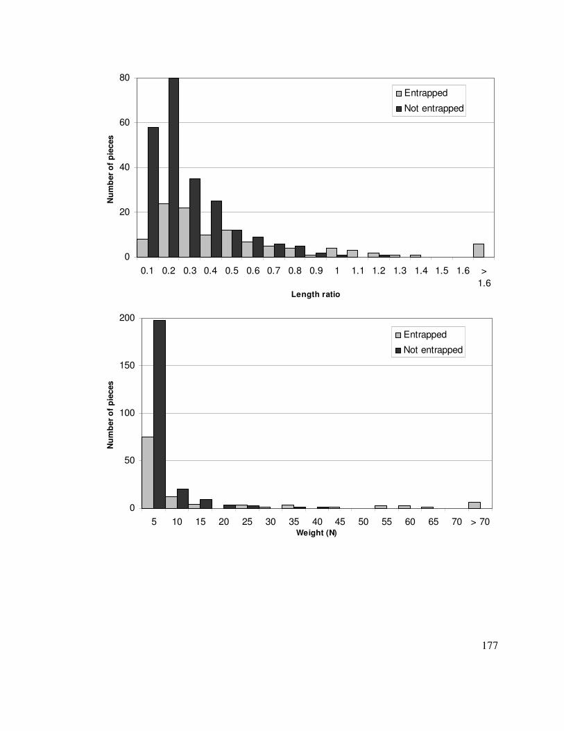
177

0

20

40

60

80

0.1 0.2 0.3 0.4 0.5 0.6 0.7 0.8 0.9 1 1.1 1.2 1.3 1.4 1.5 1.6 >

1.6Length ratio

Nu

mb

er

of

pie

ces

Entrapped

Not entrapped

0

50

100

150

200

5 10 15 20 25 30 35 40 45 50 55 60 65 70 > 70Weight (N)

Nu

mb

er

of

pie

ces

Entrapped

Not entrapped

178

0

40

80

120

160

2.5 5 7.5 10 12.5 15 17.5 20 22.5 25 27.5 30 32.5 35 > 35

Branching complexity

Nu

mb

er

of

pie

ce

s

Not entrapped

Entrapped