Review Linking climate change modelling to impacts studies ...climateknowledge.org/downscaling/Fowler_Review_Downscaling_Hydrology_IntJClimatology...modelling is reviewed in “Downscaling

INTERNATIONAL JOURNAL OF CLIMATOLOGYInt. J. Climatol. 27: 1547–1578 (2007)Published online 14 September 2007 in Wiley InterScience(www.interscience.wiley.com) DOI: 10.1002/joc.1556

Review

Linking climate change modelling to impacts studies: recentadvances in downscaling techniques for hydrological

modelling

H. J. Fowler,a* S. Blenkinsopa and C. Tebaldiba Water Resource Systems Research Laboratory, School of Civil Engineering and Geosciences, Newcastle University, UK

b Institute for the Study of Society and Environment, National Center for Atmospheric Research, Boulder, CO, USA

Abstract:There is now a large published literature on the strengths and weaknesses of downscaling methods for different climaticvariables, in different regions and seasons. However, little attention is given to the choice of downscaling method whenexamining the impacts of climate change on hydrological systems. This review paper assesses the current downscalingliterature, examining new developments in the downscaling field specifically for hydrological impacts. Sections focus on thedownscaling concept; new methods; comparative methodological studies; the modelling of extremes; and the applicationto hydrological impacts.

Consideration is then given to new developments in climate scenario construction which may offer the most potentialfor advancement within the ‘downscaling for hydrological impacts’ community, such as probabilistic modelling, patternscaling and downscaling of multiple variables and suggests ways that they can be merged with downscaling techniquesin a probabilistic climate change scenario framework to assess the uncertainties associated with future projections. Withinhydrological impact studies there is still little consideration given to applied research; how the results can be best used toenable stakeholders and managers to make informed, robust decisions on adaptation and mitigation strategies in the face ofmany uncertainties about the future. It is suggested that there is a need for a move away from comparison studies into theprovision of decision-making tools for planning and management that are robust to future uncertainties; with examinationand understanding of uncertainties within the modelling system. Copyright 2007 Royal Meteorological Society

KEY WORDS downscaling; climate change; hydrological impacts; comparative studies; extremes; uncertainty

Received 6 October 2006; Revised 27 March 2007; Accepted 6 April 2007

INTRODUCTION

General circulation models (GCMs) are an important toolin the assessment of climate change. These numericalcoupled models represent various earth systems includingthe atmosphere, oceans, land surface and sea-ice and offerconsiderable potential for the study of climate change andvariability. However, they remain relatively coarse in res-olution and are unable to resolve significant subgrid scalefeatures (Grotch and MacCracken, 1991) such as topog-raphy, clouds and land use. For example, the HadleyCentre’s HadCM3 model is resolved at a spatial resolu-tion of 2.5° latitude by 3.75° longitude whereas a spatialresolution of 0.125° latitude and longitude is required byhydrologic simulations of monthly flow in mountainouscatchments (Salathe, 2003). Bridging the gap betweenthe resolution of climate models and regional and local

* Correspondence to: H. J. Fowler, Water Resource Systems ResearchLaboratory, School of Civil Engineering and Geosciences, CassieBuilding, Newcastle University, Newcastle upon Tyne, NE1 7RU, UK.E-mail: [email protected]

scale processes represents a considerable problem forthe impact assessment of climate change, including theapplication of climate change scenarios to hydrologicalmodels. Thus, considerable effort in the climate commu-nity has focussed on the development of techniques tobridge the gap, known as ‘downscaling’.

A number of papers have previously reviewed down-scaling concepts, including Hewitson and Crane (1996);Wilby and Wigley (1997); Zorita and von Storch (1997);Xu (1999); Wilby et al. (2004); and regionally for Scan-dinavia in Hanssen-Bauer et al. (2005). This paper differsfrom previous reviews as it focuses on recent develop-ments in downscaling methods for hydrological impactstudies, updating and extending the methodological studyof Xu (1999). In the next two sections the concept ofdownscaling, the development of new methods, com-parative methodological studies and the modelling ofextremes are discussed. The application of downscalingto the field of climate change impacts on hydrologicalmodelling is reviewed in “Downscaling for hydrologi-cal impact studies”. “Incorporating new developments”

Copyright 2007 Royal Meteorological Society

1548 H. J. FOWLER ET AL.

reviews new developments in climate scenario construc-tion, such as probabilistic modelling, pattern scaling anddownscaling of multiple variables and suggests waysthat they can be merged with downscaling techniquesin a probabilistic climate change scenario framework toassess the uncertainties associated with future projec-tions. The last section “Summary and next steps” drawsthese themes together to make some recommendationson future work in the field, providing an example ofhow probabilistic climate scenarios can be linked withdownscaling methods for hydrological, and other, impactstudies.

In particular, this review will try to answer fivequestions that we believe must be addressed for thesuccessful use of downscaling methods in hydrologicalimpact assessment, in both the downscaling researchcommunity and for practitioners:

1. What more (if anything) can be learnt from downscal-ing method comparison studies?

2. Can dynamical downscaling contribute advantagesthat can not be conferred by statistical downscaling?

3. Can realistic climate change scenarios be producedfrom dynamically downscaled output for periods out-side the time period of simulation using methods suchas pattern scaling?

4. What new methods can be used together withdownscaling to assess uncertainties in hydrologicalresponse?

5. How can downscaling methods be better utilizedwithin the hydrological impacts community?

Whilst this review aims to discuss recent developmentsin the application of climate change scenarios, throughdownscaling methods, to assess hydrological impacts, itwill not provide a comprehensive review of all publishedstudies. Instead it aims to concentrate on those studies

that address new concepts and real advances in downscal-ing for hydrological impact assessment, particularly thosethat address the quantification of uncertainty in the esti-mation of climate change impacts. Therefore, the reviewwill concentrate on studies that compare different down-scaling approaches, the outputs from multiple climatemodels or ensembles, and multiple emissions scenarios.

OVERVIEW OF DOWNSCALING METHODS

Two fundamental approaches exist for the downscalingof large-scale GCM output to a finer spatial resolution.The first of these is a dynamical approach where a higher-resolution climate model is embedded within a GCM. Thesecond approach is to use statistical methods to establishempirical relationships between GCM-resolution climatevariables and local climate. These two approaches aredescribed below and the main advantages and limitationsof each are summarized in Table I.

Dynamical downscaling

Dynamical downscaling refers to the use of regional cli-mate models (RCMs), or limited-area models (LAMs).These use large-scale and lateral boundary conditionsfrom GCMs to produce higher resolution outputs. Theseare typically resolved at the ∼0.5° latitude and longitudescale and parameterize physical atmospheric processes.Thus, they are able to realistically simulate regionalclimate features such as orographic precipitation (e.g.Frei et al., 2003), extreme climate events (e.g. Fowleret al., 2005a; Frei et al., 2006) and regional scale climateanomalies, or non-linear effects, such as those associ-ated with the El Nino Southern Oscillation (e.g. Leunget al., 2003a). However, model skill depends strongly onbiases inherited from the driving GCM and the presenceand strength of regional scale forcings such as orog-raphy, land-sea contrast and vegetation cover. Studies

Table I. Comparative summary of the relative merits of statistical and dynamical downscaling techniques (adapted from Wilbyand Wigley, 1997).

Statistical downscaling Dynamical downscaling

Advantages • Comparatively cheap and computationally efficient• Can provide point-scale climatic variables fromGCM-scale output• Can be used to derive variables not available fromRCMs• Easily transferable to other regions• Based on standard and accepted statistical procedures• Able to directly incorporate observations into method

• Produces responses based on physicallyconsistent processes• Produces finer resolution information fromGCM-scale output that can resolve atmosphericprocesses on a smaller scale

Disadvantages • Require long and reliable observed historical dataseries for calibration• Dependent upon choice of predictors• Non-stationarity in the predictor-predictandrelationship• Climate system feedbacks not included

• Computationally intensive• Limited number of scenario ensemblesavailable• Strongly dependent on GCM boundaryforcing

• Dependent on GCM boundary forcing; affected by biases in underlying GCM• Domain size, climatic region and season affects downscaling skill

Copyright 2007 Royal Meteorological Society Int. J. Climatol. 27: 1547–1578 (2007)DOI: 10.1002/joc

ADVANCES IN DOWNSCALING TECHNIQUES FOR HYDROLOGICAL MODELLING 1549

within the western U.S., Europe, and New Zealand, wheretopographic effects on temperature and precipitation areprominent, often report more skilful dynamical down-scaling than in regions such as the U.S., Great Plains andChina where regional forcings are weaker (Wang et al.,2004).

Variability in internal parameterizations also providesconsiderable uncertainty. Therefore, use of model ensem-bles is to be recommended for a realistic assessment ofclimate change. Hagemann et al. (2004) examined therelative performance of four RCMs (HIRHAM, CHRM,REMO and HadRM3H) and a variable resolution GCM(ARPEGE) over the Danube and Baltic Sea catchments.Boundary conditions from gridded reanalysis data wereused to remove the effect of errors in GCM boundary con-ditions, and therefore identify simulation errors resultingfrom internal RCM parameterizations. Over the Baltic, allmodels overestimated precipitation, except in summer;probably due to inaccurate parameterizations of large-scale condensation and convection schemes. For the morecontinental Danube, all models except ARPEGE simu-lated a dry summer bias. In CHRM this was related topoor soil parameterization but in the other models it wasdue to lack of moisture advection into the region. Addi-tional errors were noted to result from poor simulation ofsnow-albedo feedback.

As dynamical downscaling is computationally expen-sive, model integrations have, until recently, beenrestricted to ‘time slices’; normally ∼30 years for a con-trol or ‘baseline’ climate from 1961–1990 and for achanged climate from 2070–2100. This makes climatechange impacts for other periods difficult to assess. Pro-ducing scenarios for other periods has been addressedusing ‘pattern scaling’ (further discussed in the section“Pattern scaling”) – where changes are scaled accordingto the temperature signal modelled for the interveningperiod, assuming a linear pattern of change (e.g. Prud-homme et al., 2002). However, some transient RCM sim-ulations, from 1950 to 2100, are now becoming available(Erik Kjellstrom, personal communication) and so thisscaling issue may soon be overcome.

Using a RCM provides additional uncertainty to thatinherent to GCM output. Uncertainty in RCM formula-tion has a small, but non-negligible, impact on futureprojections of UK and Ireland mean-climate (Rowell,2006; Fowler and Blenkinsop, in press). For tempera-ture projections, the uncertainty introduced by the RCMis less than that from the emissions scenario, but for pre-cipitation projections the opposite is true. However, thelargest source of uncertainty derives from the structureand physics of the formulation of the driving GCM. Theuncertainty introduced by ten RCMs for eight Europeanregions was evaluated by Deque et al. (2005) using RCMensemble runs and applying the same emissions scenario.The contribution of different sources of uncertainty wasfound to vary according to spatial domain, region andseason, but the largest uncertainty was introduced by theboundary forcing i.e. choice of driving GCM, particularlyfor temperature. Exceptionally, for summer precipitation

the uncertainty attributable to the choice of RCM was ofthe same magnitude.

There has now been much assessment of the abilityof RCMs to simulate climate variables, particularly thoserelevant to hydrological impact studies. Several studies(e.g. Leung et al., 2004) have illustrated how dynami-cal downscaling provides ‘added value’ for the study ofclimate change and its potential impacts, as regional cli-mate change signals can be significantly different fromthose projected by GCMs because of orographic forcingand rain-shadowing effects. Dynamical downscaling canalso provide improved simulation of meso-scale precipi-tation processes and thus higher moment climate statistics(Schmidli et al., 2006); producing more plausible climatechange scenarios for extreme events and climate vari-ability at the regional scale. To this end, longer duration,higher spatial resolution (e.g. Christensen et al., 1998),and ensemble RCM simulations (e.g. Leung et al., 2004),particularly the European FP5 Prediction of Regional sce-narios and Uncertainties for defining European Climatechange risks and Effects (PRUDENCE) project (Chris-tensen et al., 2007) and the North American Regional Cli-mate Change Assessment Program (NARCCAP) project(Mearns et al., 2006), are becoming more common.These improve the realism of control simulations; moreaccurate variability and extreme event statistics are sim-ulated by higher spatial and temporal resolution mod-els (e.g. Frei et al., 2006). Applications to geographi-cally diverse regions and model inter-comparison studieshave allowed the strengths and weaknesses of dynamicaldownscaling to be better understood (Wang et al., 2004).This has recently proliferated their use in impact stud-ies (e.g. Bergstrom et al., 2001; Wood et al., 2004; Zhuet al., 2004; Graham et al., 2007 a,b); and is further dis-cussed in “Downscaling for hydrological impact studies”.

Statistical downscaling

Many statistical downscaling techniques have been devel-oped to translate large-scale GCM output onto a finerresolution.

The simplest method is to apply GCM-scale projec-tions in the form of change factors (CFs) – the ‘perturba-tion method’ (Prudhomme et al., 2002) or ‘delta-change’approach. Differences between the control and futureGCM simulations are applied to baseline observations bysimply adding or scaling the mean climatic CF to eachday. Therefore, it can be rapidly applied to several GCMsto produce a range of climate scenarios but has a numberof caveats. Firstly, the method assumes that GCMs moreaccurately simulate relative change than absolute values,i.e. assuming a constant bias through time. Secondly, CFsonly scale the mean, maxima and minima of climaticvariables, ignoring change in variability and assumingthe spatial pattern of climate will remain constant (Diaz-Nieto and Wilby, 2005). Furthermore, for precipitationthe temporal sequence of wet days is unchanged, whenchange in wet and dry spells may be an important compo-nent of climate change. Several modifications have been



proposed. Prudhomme et al. (2002) suggest any increasein precipitation is distributed evenly among existing raindays, added to make each third dry day wet, or distributedon only the three wettest days to simulate an increase inextremes. The effectiveness of these arbitrary parametersis however, not assessed. Harrold and Jones (2003) rankGCM daily rainfall for current and future climates anduse these to scale ranked historical precipitation series, avariation which is sensitive to change in extreme rainfalland wet day frequencies.

More sophisticated statistical downscaling methods aregenerally classified into three groups:

• Regression models• Weather typing schemes• Weather generators (WGs)

Each group covers a range of methods, all relyingon the fundamental concept that regional climates arelargely a function of the large-scale atmospheric state.This relationship may be expressed as a stochastic and/ordeterministic function between large-scale atmosphericvariables (predictors) and local or regional climate vari-ables (predictands). Predictor variables useful for down-scaling typically represent the large-scale circulation, e.g.sea-level pressure and geopotential heights, but can alsoinclude measures of humidity and simulated surface cli-mate variables such as GCM precipitation and tempera-ture (e.g. Widmann and Bretherton, 2000; Salathe, 2005).Essentially, in these methods, the regional climate is con-sidered to be conditioned by the large-scale climate statein the form R = F(X), where R represents the local cli-mate variable that is being downscaled, X is the set oflarge-scale climate variables and F is a function whichrelates the two and is typically established by trainingand validating the models using point observations orgridded reanalysis data. Performance of these methodsin reproducing observed or reanalysis statistics is nor-mally measured using correlation coefficients, distancemeasures such as root mean squared error (RMSE), orexplained variance, although Busuioc et al. (2001) sug-gest that for climate change applications the optimumdownscaling model may well be that which best repro-duces low frequency variability (e.g. Wilby et al., 2002a).

Several key assumptions are inherent within these sta-tistical downscaling techniques. Firstly, predictor vari-ables should be physically meaningful, reproduced wellby the GCM and able to reflect the processes respon-sible for climatic variability on a range of timescales.For example, downscaling which uses only circulation-based predictors may fail to reflect change in atmospherichumidity in a warmer climate. Secondly, the predic-tor–predictand relationship is assumed to be stationaryin time, remaining the same in a changed future cli-mate. This assumption has shown to be questionable inthe observed record (e.g. Huth, 1997; Slonosky et al.,2001; Fowler and Kilsby, 2002) and is best tested using

long records or model validation on a period with differ-ent climate characteristics (Charles et al., 2004). Non-stationarity may be attributed to an incomplete set ofpredictor variables that exclude low-frequency climatebehaviour, inadequate sampling or calibration period, ortemporal change in climate system structures (Wilby,1998). The degree of non-stationarity in projected climatechange has recently been assessed by Hewitson and Crane(2006) who found that this is relatively small and thatcirculation dynamics in particular may be more robust tonon-stationarities.

Choice of predictor variables should also be given highconsideration. A predictor may not appear significantwhen developing a downscaling model under present cli-mate, but future changes in that predictor may be criticalin determining climate change (Wilby, 1998). For exam-ple, local temperature change under a 2 × CO2 scenario isdominated by change in atmospheric radiative propertiesrather than circulation changes (Schubert, 1998) but forlocal precipitation change the inclusion of low-frequencyatmospheric predictors can produce enhanced simulations(Wilby, 1998). There is little consensus on the mostappropriate choice of predictor variables. Circulation-related predictors, such as sea-level pressure, are attrac-tive as relatively long observations are available andGCMs simulate these with some skill (Cavazos andHewitson, 2005). However, it is increasingly acknowl-edged that circulation predictors alone are unlikely to besufficient, as they fail to capture key precipitation mech-anisms based on thermodynamics and vapour content.Thus humidity has increasingly been used to downscaleprecipitation (e.g. Karl et al., 1990; Wilby and Wigley,1997; Murphy, 2000; Beckmann and Buishand, 2002);particularly as it may be an important predictor under achanged climate. Indeed, the inclusion of moisture vari-ables as predictors can lead to convergence in the resultsof statistical and dynamical approaches (Charles et al.,1999), with the inclusion of GCM precipitation as a pre-dictor also improving downscaling skill (Salathe, 2003;Widmann et al., 2003). Cavazos and Hewitson (2005)have performed the most comprehensive assessment ofpredictor variables to date, assessing 29 NCEP reanalysisvariables using an artificial neural network (ANN) down-scaling method in 15 locations. Predictors representingmid-tropospheric circulation (geopotential heights) andspecific humidity were found to be useful in all locationsand seasons. Tropospheric thickness and surface merid-ional and mid-tropospheric wind components were alsoimportant predictors but more regionally and seasonallydependent.

The results of statistical downscaling are also depen-dent upon the choice of predictor domain (Wilbyand Wigley, 2000). However, this is generally ignored(Benestad, 2001). A study by Brinkmann (2002) sug-gests that, for studies where only one grid point is used,the optimum grid point location for downscaling may bea function of the timescale under consideration and isnot necessarily related solely to location. Additionally,large-scale circulation patterns over the predictor domain



may not capture small-scale processes; these may resultfrom variability in neighbouring locations. Similar resultswere obtained by Wilby and Wigley (2000) who foundthat in many cases, maximum correlations between pre-cipitation and mean sea level pressure (MSLP) occurredaway from the grid box, suggesting that the choice ofpredictor domain, in terms of location and spatial extent,is a critical factor affecting the realism and stability ofdownscaled precipitation scenarios.

Statistical methods are more straightforward thandynamical downscaling but tend to underestimate vari-ance and poorly represent extreme events. Regressionmethods and some weather-typing approaches under-predict climate variability to varying degrees, since onlypart of the regional and local climate variability is relatedto large-scale climate variations. Three approaches toadd variability to downscaled climate variables are fre-quently employed: variable inflation, expanded down-scaling and randomization. Variable inflation (Karl et al.,1990) increases variability by multiplying by a suitablefactor. However, von Storch (1999) suggests that variableinflation is not meaningful as it assumes that all climatevariability is related to the large-scale predictor fields,recommending the alternative approach of ‘randomiza-tion’ where additional variability is added in the formof white noise (e.g. Kilsby et al., 1998). This was foundto give good results in the reproduction of 20–50 yearreturn values of central European surface temperature(Kysely, 2002). The more sophisticated ‘expanded down-scaling’ approach, a variant of canonical correlation anal-ysis (CCA), was developed by Burger (1996) and hasbeen used by Huth (1999); Dehn et al. (2000) and Muller-Wohlfeil et al. (2000). A comparison of the three methodsnotes that each presents different problems (Burger andChen, 2005). Variable inflation poorly represents spa-tial correlations, whilst randomization performs well forcontrol climate simulations but is unable to reproducechanges in variability which may represent a significantdisadvantage given the expectations of future change. Incontrast, expanded downscaling is sensitive to the choiceof statistical process used during its application.

Regression models. The term ‘transfer function’ (Giorgiand Hewitson, 2001) is used to describe methods thatdirectly quantify a relationship between the predictandand a set of predictor variables. In the simplest form,multiple regression models are built using grid cell val-ues of atmospheric variables as predictors for surfacetemperature and precipitation (e.g. Hanssen-Bauer andFørland, 1998; Hellstrom et al., 2001). Other more com-plex techniques include using the principal componentsof pressure fields or geopotential heights (e.g. Cubaschet al., 1996; Kidson and Thompson, 1998; Hanssen-Bauer et al., 2003) and more sophisticated methods suchas ANNs (e.g. Zorita and von Storch, 1999), CCA (Karlet al., 1990; Wigley et al., 1990; von Storch et al., 1993;Busuioc et al., 2001) and singular value decomposition(SVD) (Huth, 1999; von Storch and Zwiers, 1999).

There have been a number of recent innovations inthis type of downscaling. For example, Abaurrea andAsın (2005) applied a logistic regression model to dailyprecipitation probability and a generalized linear modelfor wet day amounts for the Ebro Valley, Spain. Theapproach simulated seasonal characteristics and someaspects of daily behaviour such as wet and dry runs well,but had low skill in reproducing extreme events. Bergantand Kajfez-Bogataj (2005) used multi-way partial leastsquares regression to downscale temperature and pre-cipitation in Slovenia, more appropriate with predictorvariables that are strongly correlated. The method per-formed better than a more conventional method based onregression of principal components but was tested onlyon the cold season.

Weather typing schemes. Weather typing or classifica-tion schemes relate the occurrence of particular ‘weatherclasses’ to local climate. Weather classes may be definedsynoptically, typically using emprical orthogonal func-tions EOFs from pressure data (Goodess and Palutikof,1998), by indices from SLP data (e.g. Conway et al.,1996), or by applying cluster analysis (Fowler et al.,2000, 2005b) or fuzzy rules (Bardossy et al., 2002, 2005)to atmospheric pressure fields. Local surface variables,typically precipitation, are conditioned on daily weatherpatterns by deriving conditional probability distributionsfor observed statistics, e.g. p(wet–wet) or mean wetday amount, associated with a given atmospheric circu-lation pattern (e.g. Bellone et al., 2000). Climate changeis estimated by evaluating the change in the frequency ofthe weather classes simulated by the GCM. The methodassumes that the characteristics of the weather classes willnot change and many classification procedures also havethe inherent problem of within-class variability of cli-mate parameters (Brinkmann, 2000). Enke et al. (2005a)recently described a scheme to partially address this,limiting within-type variability by deriving a classifica-tion scheme for circulation patterns that optimally dis-tinguishes between different values of regional weatherelements. The scheme is based on a stepwise multipleregression where predictor fields are sequentially selectedto minimize the RMSE between forecasts and observa-tions. This is applied in Enke et al. (2005b) with the aimof modelling daily extremes of not yet observed magni-tudes. This uses a two-stage process; first applying thecirculation pattern frequencies from the model and thenusing regression analysis to make alterations resultingfrom changes in the intensity of atmospheric processes,for example increasing geopotential thicknesses.

Weather generators. At their simplest these are stochas-tic models, based on daily precipitation with a two-state first-order Markov chain dependent on transi-tion probabilities for simulating precipitation occurrence,and a gamma distribution for precipitation amounts(e.g. WGEN, Wilks, 1992), although second-order (e.g.Mason, 2004) and third-order (e.g. MetandRoll;Dubrovsky et al., 2004) Markov chain models have now



been developed that are better able to reproduce precipi-tation occurrence or persistence. Rather than being con-ditioned by weather patterns, variables are conditionedon specific climatic events, e.g. precipitation occurrence,with daily climate governed by the outcome on pre-vious days. An example is the climate research unit(CRU) daily WG developed by Jones and Salmon (1995)and modified by Watts et al. (2004). It generates pre-cipitation using a first-order Markov chain model fromwhich other variables – minimum and maximum tem-peratures, vapour pressure, wind speed and sunshineduration – are generated. A recent development of thisapproach has been the linkage of a stochastic precipitationgenerator – the Neyman Scott rectangular pulses (NSRP)model – to the weather component developed by Wattset al. (2004). This is described in Kilsby et al. (2007b)and has been shown to improve upon the Markov chainmodel approach; better describing both variability andextremes within climatic time series.

WGs may also be driven by a weather typing scheme.Corte-Real et al. (1999) used daily weather patterns iden-tified from principal components of MSLP to conditiona WG. Improvements in the modelling of the autocorre-lation structure of wet and dry days were observed whenthe probability of rain is conditioned on the current cir-culation pattern and the weather regime of the previousday. The generator simulated fundamental characteristicsof precipitation such as the distribution of wet and dryspell lengths and even extreme precipitation. Other stud-ies have also found that conditioning on circulation andlow frequency variability, including sea-surface temper-atures (SSTs), improves simulation results (e.g. Wilbyet al., 2002a).

The relative performance of different WGs wasassessed by Semenov et al. (1998) who indicated thatLARS-WG (Racsko et al., 1991) is better than WGEN atreproducing monthly temperature and precipitation meansacross the USA, Europe and Asia due to a greater numberof parameters and the use of more complex distributions.However, both were poor at modelling inter-annual vari-ability in monthly means and reproducing frost and hotspells due to simplistic treatment of persistence. Qianet al. (2005) evaluated the LARS-WG and AAFC-WG(Hayhoe, 2000) WGs and highlighted differences in per-formance; most notably that the AAFC-WG model wasbetter at reproducing distributions of wet and dry spellsthan the LARS-WG.

The major disadvantage of WGs is that they are con-ditioned using local climate relationships and so may notbe automatically applicable in other climates, though theextent to which this limits their usefulness has not beenfully tested. They also tend to underestimate inter-annualvariability. Approaches have been developed to improvethe simulation of variability. For example, the incorpora-tion of a stochastic rainfall model into a WG (e.g. Kilsbyet al., 2007b) improves the simulation of both variabil-ity and extremes when compared to the use of a sim-ple Markov method. Additionally, Wilby et al. (2002b)developed the Statistical DownScaling Model (SDSM),

a hybrid of stochastic WG and regression methods. Ituses circulation patterns and moisture variables to condi-tion local weather parameters, and stochastic methods toinflate the variance of the downscaled climate series.

COMPARISON OF DOWNSCALING METHODS

The section entitled “Overview of downscaling methods”has indicated that there are a wide range of downscal-ing methods that may be employed. However, the use ofdifferent spatial domains, predictor variables and predic-tands, and assessment criteria makes direct comparisonof the relative performance of different methods difficultto achieve. This represents a problem for their applicationin climate change impact assessments as the differentialperformance of each method creates a further level ofuncertainty that is difficult to quantify.

Many recent studies have compared the performanceof different downscaling methods. In this section stud-ies that have compared different statistical downscal-ing techniques and those that have examined the rel-ative performance of statistical and dynamical or sta-tistical–dynamical methods are reviewed. The Statisti-cal and Regional dynamical Downscaling of Extremesfor European regions (STARDEX) project is the firstattempt to rigorously and systematically compare statis-tical, dynamical and statistical–dynamical downscalingmethods, focussing on the downscaling of extremes, andthis is discussed further in “Downscaling of extremes”.

Inter-comparison of statistical downscaling methods

Studies comparing different statistical downscaling meth-ods are now relatively common. Most, however, investi-gate the downscaling of either precipitation or tempera-ture, with few investigating the simultaneous downscal-ing of multiple variables.

The earliest study of precipitation downscaling meth-ods (Wilby and Wigley, 1997), for six North Americanstudy regions compared the performance of two ANNmodels, two WGs – the WGEN WG based on a two-state Markov process of rainfall occurrence, and anotherbased on spell length – and two semi-stochastic classifi-cation schemes based on daily vorticity values. Fourteendiagnostic statistics were compared, including mean pre-cipitation, wet day probabilities, extreme precipitationamounts and wet and dry spell lengths. Model perfor-mance varied considerably for the statistics being tested.The WGs captured wet-day occurrence and amount butwere less skilful for inter-annual variability; with theopposite found for ANNs. Overall, WGs proved moreskilful, with ANNs the worst because of the overesti-mation of wet days; use of the direct output from theHadCM2 GCM was superior to one ANN model on 12out of 14 occasions.

Indeed, ANNs have been shown repeatedly to per-form poorly in the simulation of daily precipitation,particularly for wet-day occurrence (Wilby and Wigley,1997; Wilby et al., 1998; Zorita and von Storch, 1999;



Khan et al., 2006) due to a simplistic treatment of dayswith zero amounts, although they perform adequately formonthly precipitation (Schoof and Pryor, 2001). Harphamand Wilby (2005) addressed this by using variants ofANNs which, analogous to weather generation methods,treat the occurrence and amount of precipitation sepa-rately. These ANNs were more skilful than the SDSMfor individual sites but over-estimated inter-site correla-tions of daily amounts due to the deterministic forcing ofamounts, whereas the stochastic nature of the SDSM ledto increased heterogeneity and lower inter-site relations.

A more modest comparative study by Zorita and vonStorch (1999) concluded that simple analogue methodsperform as well as more complex methods. Analoguesreproduced the mean monthly and daily statistics ofwinter Iberian rainfall well, producing results comparableto a CCA method, and outperformed CCA and ANNs insimulating variability. Similarly, Widmann et al. (2003)found that using GCM precipitation as a predictor indownscaling improved results considerably, without theuse of complex statistical methods. This approach wasextended by Schmidli et al. (2006) to the daily temporalresolution.

Comparative studies of methods for downscaling meantemperature have also been undertaken. Huth (1999)compared several linear methods for the downscaling ofdaily mean winter temperature in central Europe: CCA,SVD and three multiple regression models – stepwiseregression of principal components (PCs), and regressionof PCs with and without stepwise screening of griddedvalues. PCs without screening, including all PCs withinthe analysis, provided the greatest skill, with the othertwo regression methods and CCA performing with com-parable skill providing a large number of predictor PCswere used. This suggests that the stepwise screening ofpredictor variables may be an unnecessary step. Howeveras GCMs simulate predictors with differing accuracy, therating of methods may have been different had down-scaling been applied to a GCM control run rather thanNCEP reanalyses. Note also that as winter temperaturesare relatively straightforward to downscale then it is ques-tionable as to how much variation in skill is linked to thedownscaling methodology.

Benestad (2001) compared methods for downscalingmonthly mean temperature: EOFs and a conventionalCCA method. Using EOFs was found to be more robustwith respect to predictor domain as it reduced the numberof subjective choices for model set up; therefore moreappropriate for downscaling global climate scenarios.To downscale maximum temperature series, Schoof andPryor (2001) compared ANNs with regression methodsfor a station in Indianapolis, U.S. The ANNs proved moreskilful if lagged predictors were not included.

Downscaling method comparisons for more than onevariable are rare. Dibike and Coulibaly (2005) comparedSDSM, and a stochastic WG (LARS-WG) for a catch-ment in northern Quebec. Mean daily precipitation was

simulated well by both methods; the WG better repro-duced wet and dry-spell lengths, with SDSM underes-timating wet-spell lengths. For maximum and minimumtemperatures both models performed well, with SDSMshowing a consistent cold bias and LARS-WG show-ing positive and negative biases in different months. Forfuture scenarios however, the models displayed differ-ent results. SDSM simulated a generally increasing trendin mean daily precipitation amount and variability notreproduced by the WG. Similar results were obtained byKhan et al. (2006) in a comparison of SDSM, LARS-WGand an ANN method. SDSM was found to performthe best, with the ANN method producing the poorestresults. SDSM has also been compared with the pertur-bation method in the Thames Valley, UK (Diaz-Nietoand Wilby, 2005). SDSM modelled monthly totals andwet day occurrence reasonably well but underestimateddry spell length. Despite the inclusion of a lagged predic-tor, the persistence of the precipitation process was notcaptured well.

Relative performance of dynamical and statisticalmethods

There have been few studies of the relative performanceof dynamical and statistical methods in climate changeimpact assessment. Kidson and Thompson (1998) com-pared the performance of the regional atmospheric mod-elling system (RAMS), RCM and a regression-basedmethod for New Zealand. Their technique used fiveEOFs of geopotential height and other derived vari-ables as predictors for daily temperature and precipita-tion. They noted little difference in skill for daily ormonthly timescales. The dynamical RAMS model hasgreater skill in simulating convective precipitation butoverall the relative computational efficiency favoured thestatistical model. Murphy (1999) drew similar conclu-sions for Europe using the UK meteorological officeunified model RCM and a regression method. However,applying the same methods to a future scenario (Murphy,2000) produced divergent results for the dynamical andstatistical methods. Calibrating the regression equationsusing GCM-simulated variables rather than observationshighlighted differences in the strength of the predictor-predictand relationship in the model. Mearns et al. (1999)also observed large differences in projections for climatechange scenarios for east Nebraska despite similar skillfor current climate conditions when using the RegCM2RCM and a statistical technique based on stochastic gen-eration conditioned upon weather types. Climate changebeyond the range of the data used to condition the modelwas hypothesized as a possible reason for this difference.

Hellstrom et al. (2001) compared dynamical outputsfrom the Rossby Centre RCM (RCA1) driven by twodifferent GCMs (HadCM2 and ECHAM4/OPYC3) withregression models based on large-scale circulation indicesand including a humidity measure. All downscaling meth-ods improved the simulation of the seasonal cycle andstatistical and dynamical methods driven by ECHAM4showed higher simulation skill. When applied to a future



scenario, differences between the two statistical meth-ods were larger than differences between dynamical andstatistical methods.

Wilby et al. (2000) examined the performance of statis-tical and dynamical methods in a mountainous catchmentusing the Animas basin, Colorado. Temperature, precip-itation occurrence and amount were downscaled using amultiple regression method. Overall, statistical downscal-ing had greater skill in simulating maximum and mini-mum temperatures than precipitation. Uncorrected RCMmonthly temperatures showed a cold bias in maximumtemperature. RCM results could however be improvedby providing an elevational bias correction on the rawRCM output. Similar conclusions were derived by com-paring dynamically and statistically downscaled precipi-tation and temperature time series for three mountainousbasins in Washington, Colorado and Nevada, USA (Hayand Clark, 2003).

Haylock et al. (2006) compared six statistical and twodynamical downscaling methods with regard to their abil-ity to downscale seven indices of heavy precipitation fortwo station networks in northwest and southeast Eng-land. Generally, winter showed the highest downscalingskill and summer the lowest; skill increases as the spa-tial coherence of rainfall increases. Indices indicative ofrainfall occurrence processes were also found to be bet-ter modelled than those indicative of intensity. Methodsbased on non-linear ANNs were found to be the bestat modelling the inter-annual variability but these had astrong negative bias in the estimation of extremes; cir-cumvented by the development of a novel re-samplingmethod. Similar results to Murphy (2000) and Hellstromet al. (2001) were obtained when applying six of themethods to the HadAM3P model forced by two differentemissions scenarios. The inter-method differences in thefuture change estimates for precipitation indices were atleast as large as the differences between the emissionsscenarios for a single method.

There have also been comparisons of statistical anddynamical downscaling methods within the seasonal fore-casting field. Dıez et al. (2005) compared their perfor-mance in downscaling seasonal precipitation forecastsover Spain from two DEMETER models: ECMWF andUKMO. As with similar studies in the climate changeliterature, they conclude that different methods producebetter results dependent upon season and on the studyregion.

The performance of the direct statistical downscalingof GCM output has been compared with the use of anintermediate dynamical downscaling step before statis-tical downscaling. Hellstrom and Chen (2003) used athree-step method to downscale Swedish precipitation.RCM predictors (using RCA1) were up-scaled to GCMlevel (HadCM2 and ECHAM4) using a linear interpola-tion scheme based on the assumption that the inclusionof small-scale information in the large-scale field shouldhave positive effects. These were then downscaled usinga multiple regression model. The intermediate dynami-cal downscaling step improved the seasonal cycle of the

predictors but only provided a slight improvement in theseasonal cycle of precipitation; not a reasonable returnon the cost of running the regional models. Wood et al.(2004) came to similar conclusions in a comparison ofsix downscaling approaches to produce precipitation andother variables for hydrological simulation. Three rel-atively simple statistical downscaling methods – linearinterpolation, spatial disaggregation, and bias-correctionand spatial disaggregation – were each applied to GCMoutput directly and after dynamical downscaling with aRCM. The most important aspect of use of GCM orRCM outputs was found to be the bias-correction step (asnoted by Wilby et al. (2000) and Hay and Clark (2003)).The dynamical downscaling step did not lead to largeimprovements in simulation relative to using GCM outputalone. This is in contrast to comparisons in the seasonalforecasting field (Dıez et al., 2005) where using dynam-ical and statistical downscaling methods in combinationwas found to offer an improvement over their use alone.

Downscaling performance for different climates

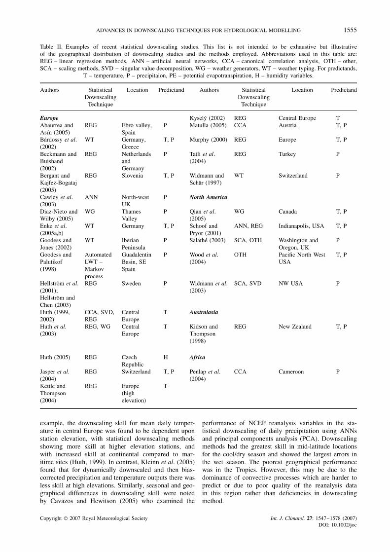
It is also difficult to assess the relative performance of dif-ferent downscaling methods in different climatic regimes,although it would be expected that different methodswould have greater skill in different climates since sea-sonal differences in simulation are noted in the com-parison studies reviewed in the earlier sections. Indeed,in some studies statistical downscaling is conducted foreach season separately because of the strong seasonallinks between large-scale circulation and local climatein the mid-latitudes (e.g. Matulla, 2005). Table II listsrecent statistical downscaling publications and their studyregions. Commonly, choice of downscaling method is notbased on any objective criteria related to either the vari-able to be downscaled or climatic region, with globalapplicability assumed (Wetterhall et al., 2006), althoughmany researchers have commented that the accuracy ofdownscaling methods has a geographical and seasonalcomponent (e.g. Huth, 1999). However, an importantcomponent of any impact study should be an assess-ment of the conditions under which different downscalingmethods can be successfully applied.

Few studies have examined whether choice of down-scaling method should be based on climatic region, down-scaled climatic variable or season. Indeed, the use ofhomogeneous climatic regions in downscaling studiesis a relatively new concept, with the prospect that sta-tistical connections between large-scale circulation andlocal climate should be more stable. This was recentlyshown to be of benefit in a region of the Tropics byPenlap et al. (2004). This spatial differentiation was alsoused in an Austrian study by Matulla (2005) whereregion- and season-specific combinations of predictorvariables were used in downscaling. Here, the use ofhomogenous regions also enhanced the performance ofthe downscaling models, although the improvement wasonly slight. Regional or seasonal dependence in down-scaling has been observed by other researchers. For



Table II. Examples of recent statistical downscaling studies. This list is not intended to be exhaustive but illustrativeof the geographical distribution of downscaling studies and the methods employed. Abbreviations used in this table are:REG – linear regression methods, ANN – artificial neural networks, CCA – canonical correlation analysis, OTH – other,SCA – scaling methods, SVD – singular value decomposition, WG – weather generators, WT – weather typing. For predictands,

T – temperature, P – precipitaion, PE – potential evapotranspiration, H – humidity variables.

Authors StatisticalDownscaling

Technique

Location Predictand Authors StatisticalDownscaling

Technique

Location Predictand

Europe Kysely (2002) REG Central Europe TAbaurrea andAsın (2005)

REG Ebro valley,Spain

P Matulla (2005) CCA Austria T, P

Bardossy et al.(2002)

WT Germany,Greece

T, P Murphy (2000) REG Europe T, P

Beckmann andBuishand(2002)

REG NetherlandsandGermany

P Tatli et al.(2004)

REG Turkey P

Bergant andKajfez-Bogataj(2005)

REG Slovenia T, P Widmann andSchar (1997)

WT Switzerland P

Cawley et al.(2003)

ANN North-westUK

P North America

Diaz-Nieto andWilby (2005)

WG ThamesValley

P Qian et al.(2005)

WG Canada T, P

Enke et al.(2005a,b)

WT Germany T, P Schoof andPryor (2001)

ANN, REG Indianapolis, USA T, P

Goodess andJones (2002)

WT IberianPeninsula

P Salathe (2003) SCA, OTH Washington andOregon, UK

P

Goodess andPalutikof(1998)

AutomatedLWT –Markovprocess

GuadalentinBasin, SESpain

P Wood et al.(2004)

OTH Pacific North WestUSA

T, P

Hellstrom et al.(2001);Hellstrom andChen (2003)

REG Sweden P Widmann et al.(2003)

SCA, SVD NW USA P

Huth (1999,2002)

CCA, SVD,REG

CentralEurope

T Australasia

Huth et al.(2003)

REG, WG CentralEurope

T Kidson andThompson(1998)

REG New Zealand T, P

Huth (2005) REG CzechRepublic

H Africa

Jasper et al.(2004)

REG Switzerland T, P Penlap et al.(2004)

CCA Cameroon P

Kettle andThompson(2004)

REG Europe(highelevation)

T

example, the downscaling skill for mean daily temper-ature in central Europe was found to be dependent uponstation elevation, with statistical downscaling methodsshowing more skill at higher elevation stations, andwith increased skill at continental compared to mar-itime sites (Huth, 1999). In contrast, Kleinn et al. (2005)found that for dynamically downscaled and then bias-corrected precipitation and temperature outputs there wasless skill at high elevations. Similarly, seasonal and geo-graphical differences in downscaling skill were notedby Cavazos and Hewitson (2005) who examined the

performance of NCEP reanalysis variables in the sta-tistical downscaling of daily precipitation using ANNsand principal components analysis (PCA). Downscalingmethods had the greatest skill in mid-latitude locationsfor the cool/dry season and showed the largest errors inthe wet season. The poorest geographical performancewas in the Tropics. However, this may be due to thedominance of convective processes which are harder topredict or due to poor quality of the reanalysis datain this region rather than deficiencies in downscalingmethod.



Goodess et al. (2007), in a comparison of 22 statisti-cal downscaling methods, as part of the FP5 STARDEXproject, found that downscaling performance was betterin winter than summer and generally better in wetter thandrier regions, probably due to the difficulty in resolv-ing small scale processes in the driest regions. However,locally-developed methods were not found to outperformmethods developed using the whole European domain,apart from for CCA. A study in China by Wetterhallet al. (2006) evaluated four statistical precipitation down-scaling methods on three catchments located in differentclimatic zones, reaching similar conclusions to Goodesset al. (2007). They used the STARDEX extreme indicesand an inter-annual variability measure to evaluate modelperformance using probability scores commonly used inforecasting. The study clearly showed that model perfor-mance was better in wetter geographical locations andthat winter precipitation is better simulated than sum-mer, due to its link to large-scale circulation patterns.Inter-annual variability was improved with the additionof humidity as a predictor variable.

The difficulties in GCM parameterization in someregions present additional problems for downscaling.For example, the different treatment of sea-ice wasconsidered an important factor in interpreting downscaledtemperature from three GCMs for Svalbard in the ArcticOcean (Benestad et al., 2002), leading them to concludethat statistical downscaling models may be invalidated infuture climates affected by nearly ice-free Arctic Oceans.

Downscaling of extremes

Most climate change research has been framed withinthe context of studies of mean global climate (e.g. Jones,1988). However, following the Intergovernmental Panelon Climate Change’s (IPCC) second assessment report(Houghton et al., 1996) which asked the question ‘Hasthe climate become more variable or extreme?’, increasedattention has focused on climate variability and possiblechanges in short-term extremes of not just temperaturebut also precipitation (Nicholls et al., 1996). Modellingevidence (e.g. Frei et al., 1998) suggests that warmingmay lead to an intensification of the hydrological cycleand increases in mean and heavy precipitation.

Change in variability and extremes may have thelargest impact on hydrological systems but extremeclimate events are not easily defined. Many studies ofextremes have focussed on what Klein Tank and Konnen(2003) refer to as ‘soft’ extremes, typically 90th or95th percentile events, principally because the detectionprobability of trends decreases for even moderatelyrare events (Frei and Schar, 2001). Other studies haveexamined more rare events, for example, events withreturn periods of 50 years (e.g. Ekstrom et al., 2005;Fowler et al., 2005a). The performance of downscalingmethods in representing extremes is therefore difficultto quantify as many different extreme thresholds havebeen assessed and, indeed, extreme climatic events in onecatchment may not be of the same magnitude as those inanother.

As the reliability of GCM output decreases withincreases in temporal and spatial resolution, the represen-tation of extremes is poor. Huth et al. (2003) found thatGCMs differ in their ability to reproduce higher ordermoments for central European temperatures. ECHAM4was able to reproduce skewness and kurtosis but CCCM2failed. GCM skill for very low and high temperatures isalso limited (Kysely, 2002). Only ECHAM4 could evenpartially reproduce extreme summer temperatures acrossthe European domain. CCCM2 also has problems repro-ducing winter temperatures due to poor soil moistureparameterization. As subgrid scale processes are moreimportant for extreme precipitation than temperature, themodelling of precipitation extremes is also poor. This hasled to the use of both dynamical and statistical methodsin the downscaling of extremes.

The ability of dynamical downscaling methods toreproduce extreme climate statistics has been assessed ina few studies concentrating on precipitation. For example,the HadRM3H regional climate model was found torepresent extreme precipitation events with return periodsof up to 50 years well for most of the UK (Fowleret al., 2005a). The main deficiencies in the model’srepresentation of extremes are related to the treatmentof orographic rainfall processes; consequently extremesin north Scotland are over estimated with the conversein eastern rain-shadowed regions. However, other RCMswere found to perform poorly in the simulation ofextreme precipitation, particularly at the 1 day level(Fowler et al., in press). Such assessments of modelperformance are crucial if they are to be applied withconfidence to the prediction of future extremes underenhanced greenhouse conditions (e.g. Ekstrom et al.,2005). However, as most uncertainty in future climate isderived from the choice of climate model and emissionsscenario (Deque et al., 2007), a better understanding ofthe range of possible future change may be derived bycomparing a number of climate models under differentemission scenarios.

Even models sharing similar parameterization schemesmay produce considerably different daily precipitationstatistics (Frei et al., 2003). Consequently, Frei et al.(2006) evaluated the performance of dynamical down-scaling of daily precipitation extremes for the EuropeanAlps using six RCMs driven by HadAM3H boundaryconditions to derive a range of estimates for future changein extremes. The models showed some skill in reproduc-ing the 5-year return value. Furthermore, model biases forthe tails of the extreme distribution were similar to thosefor wet-day intensities, suggesting errors in the extremesare related to the intensity rather than the occurrence pro-cess.

The ability of statistical downscaling methods to repro-duce extreme climate statistics has also been assessed.The most comprehensive study was performed byGoodess et al. (2007) who compared 22 statistical down-scaling methods using ten extremes indices, taking intoaccount magnitude, frequency and persistence, for sixEuropean regions and Europe as a whole. For many



indices they used percentile thresholds rather than fixedvalues, focussing on moderate extremes. This may beof limited applicability to hydrological studies whererare events are of interest. The comparison used com-mon data sets, calibration and validation periods, andtest statistics, aiming to compare systematic differencesin model performance between different seasons, indicesand regions. Comparisons were also made of differencesbetween direct methods, in which seasonal indices ofextremes are downscaled, and indirect methods, in whichdaily time series are generated and seasonal indices cal-culated.

The performance of downscaling methods variedacross seasons, stations and indices, making it difficultto identify a best method. However, traditional meth-ods, such as stepwise regression, compositing, correla-tion analysis, PCA and CCA were more useful thannovel methods such as ANNs (e.g. Harpham and Wilby,2005); although Haylock et al. (2006) developed a novelapproach within one of the ANN methods to outputthe rainfall probability and gamma distribution scaleand shape parameters for each day which allowed re-sampling methods to be used to improve the estimationof extremes. Station to station differences were foundto dominate index to index, method to method and sea-son to season differences, although methods generallyperformed better in winter than summer, particularly forprecipitation. In general, methods were found to performbetter for mean than extreme indices of temperature andprecipitation. Watts et al. (2004) presented similar con-clusions for the CRU WG for extremes based on 90thand 95th percentile values. Downscaling methods werealso shown to capture some processes better than oth-ers (Haylock et al., 2006; Goodess et al., 2007); indicesrepresenting the frequency of extremes were better repro-duced than those for the magnitude of events. Occurrenceprocesses are better captured by the downscaling pro-cess as predictors based on large-scale circulation capturethe patterns prohibiting precipitation occurrence whereasevent magnitude depends on smaller local-scale pro-cesses. Haylock et al. (2006) applied six of the methodsto the Hadley Centre global climate model HadAM3Pforced by emissions according to two SRES scenarios.This revealed that the inter-method differences betweenthe future changes in the downscaled precipitation indiceswere at least as large as the differences between theemission scenarios for a single model. Goodess et al.(2007) concluded that there was no consistently supe-rior downscaling method and recommended using a rangeof statistical downscaling methods, alongside a range ofRCMs and GCMs, for scenarios of extremes, but thatstatistical downscaling methods may be more appropri-ate where point values of extremes are needed for impactstudies.

Other researchers have also investigated statisticaldownscaling methods. Coulibaly (2004) used a geneticprogramming (GP) method to downscale local extreme(minimum and maximum) temperatures in northernCanada. The GP method was found to outperform the

SDSM approach in the simulation of temperature min-ima, but both methods performed similarly for tempera-ture maxima. Similarly, Schubert and Henderson-Sellers(1997) used a PCA of MSLP fields to derive relationshipsbetween large-scale atmospheric flow patterns and localscale temperature extremes. Huth et al. (2003) indicatedthat skewness of summer maximum and winter minimumtemperature distributions for the same region were wellreproduced by a stochastic WG (MetandRoll). However,downscaling with a regression method for winter min-ima produced the right sign skewness but not magnitudewhereas summer maxima had unrealistic negative skew-ness.

It is likely that all downscaling methods produceextremes that are too moderate compared with observedseries; possibly linked to the assumption of linearity inmost downscaling methods (Kysely, 2002). A comparisonof a stepwise regression method with outputs of twoGCMs (ECHAM4 and CCCM2) for central European 20-and 50-year return values of annual maxima by Kysely(2002) produced different results dependent on GCM.ECHAM4 GCM output was found to be better thandownscaled results, whereas downscaling from CCCMimproved the representation of extremes. Downscalingresults were also found to be worse for annual minimacompared with annual maxima as cold extremes are morestrongly influenced by radiation balance and local stationsetting than large-scale circulation factors.

Discussion of comparative studies

Consideration of these analyses suggests that, at leastfor present day climates, dynamical downscaling meth-ods provide little advantage over statistical techniques.Murphy (2000) suggests that increased confidence inRCM estimates of change will only be established byconvergence between dynamical and statistical predic-tions, or by the emergence of clear evidence supportingthe use of a single preferred method. This, however, pre-supposes that such a method will emerge. Comprehensivecomparison studies such as STARDEX suggest that noone method is better and thus it may be more appro-priate to pursue an approach based on the constructionof probabilistic scenarios as discussed in “Probabilisticprojections of climate change”.

DOWNSCALING FOR HYDROLOGICAL IMPACTSTUDIES

GCMs were not designed for the application of hydro-logical responses to climate change. GCM-predicted run-off is over-simplified and lacks a lateral transfer ofwater within the land phase between grid cells (Xu,1999), although results vary considerably between mod-els (Wilby et al., 1999). Additionally, off-line hydrolog-ical models driven directly by GCM output have beenfound to perform poorly; the quality of GCM outputsprecluding their direct use for hydrological impact stud-ies (Prudhomme et al., 2002). A clear mismatch exists



between climate and hydrologic modelling in terms ofthe spatial and temporal scales, and between GCM accu-racy and the hydrological importance of the variables. Inparticular, the reproduction of observed spatial patternsof precipitation (Salathe, 2003) and daily precipitationvariability (Burger and Chen, 2005) is not sufficient.However improved results can be obtained by the appli-cation of even simple downscaling methods (Wilby et al.,1999)

The downscaling of climate model outputs to studythe hydrological consequences of climate change is nowcommon. However, the minimum standard for any use-ful downscaling procedure for hydrological applicationsis that ‘the historic (observed) conditions must be repro-ducible’ (Wood et al., 2004). The simplest methodsexamine hypothetical climate change scenarios by mod-ifying time series of meteorological variables by CFsin accordance with GCM scenario results, often on amonthly basis (e.g. Arnell and Reynard, 1996; Boormanand Sefton, 1997). However, these do not allow forchange in temporal variability (Kilsby et al., 1998; asdiscussed in “Relative performance of dynamical andstatistical methods”) and so recent studies have usedmore sophisticated methods. Hydrological climate changeimpact studies have used dynamically downscaled out-put directly (Wood et al., 2004; Graham et al., 2007a,b),bias-corrected dynamically downscaled output (Woodet al., 2004; Fowler and Kilsby, 2007; Fowler et al.,2007), simple statistical approaches such as multipleregression relationships (e.g. Wilby et al., 2000; Jasperet al., 2004), expanded downscaling (Muller-Wohlfeilet al., 2000), stochastic WGs (e.g. Evans and Schreider,2002), statistical links to weather typing and circulationindices (e.g. Pilling and Jones, 2002), and some studieshave compared more than one approach.

Comparison of downscaling approaches

The relative performance of different downscaling meth-ods for hydrological impact assessment has been assessedby a few studies. Wilby et al. (2000) examined the perfor-mance of statistical and dynamical methods in mountain-ous areas using data from the Animas basin in Colorado.Temperature, precipitation occurrence and amount weredownscaled using a multiple regression method. Overall,statistical downscaling returned better results than RCMoutput for daily run-off due to well timed snow packmelt. This was found to be regulated by temperatureand estimates of gross snow pack accumulation ratherthan the sequence of individual precipitation events. Theresults could still be improved by using an elevationbias correction on the raw RCM output however. Similarconclusions were derived by Hay and Clark (2003) forthree mountainous basins in Washington, Colorado andNevada, U.S. However, Kleinn et al. (2005) found that byusing bias-corrected RCM output at 56- and 14-km gridresolution they were able to reproduce monthly stream-flow variability in the Rhine basin, although the modelperformed more poorly at high elevations. Model resolu-tion was found to have a limited impact upon streamflow

simulation in large catchments, but may have a significantimpact in small catchments.

However, in catchments where run-off is not snow-melt driven, other climatic features important for hydro-logical impacts may be poorly captured by statisti-cal downscaling methods. For example, Diaz-Nieto andWilby (2005) demonstrated in the River Thames, UK,that the SDSM underestimates mean dry-spell length.This reflects its inability to capture the true persistence ofthe precipitation occurrence process. Comparisons of sta-tistical downscaling methods have also been made, withthe use of different downscaling methods resulting insignificantly different hydrological impacts for the samecatchment (Coulibaly et al., 2005; Dibike and Coulibaly,2005). The implication of such studies for future down-scaling for hydrological impacts assessment is that themeans by which downscaling skill is assessed must betuned to the particular catchment and application in ques-tion rather than simply applying standard assessment cri-teria.

Simple methods have also been used for downscalingand found to be effective in simulating hydrological sys-tems. A comparative assessment of precipitation down-scaling methods was undertaken by Salathe (2003) for theYakima River, Washington. In this area many events areassociated with large-scale storm systems; downscalingmust reflect the physical processes accounting for precip-itation. They assessed the performance of applying a localscaling factor compared to a ‘dynamical scaling’ method;a modification of the local scaling method that takesaccount of atmospheric circulation being dependent onmonthly mean 1000 hPa heights. This ‘dynamical scal-ing’ produced significant improvement in simulation inthe lee of the Cascade Mountains, which are not resolvedin a GCM, but little difference in other areas. Both meth-ods were able to simulate inter-annual flow variabilityand capture wet and dry sequences. In the simulation ofmonthly flows, local scaling was even able to differen-tiate between years with double-peaked flow and yearswith a single, melt-driven peak; a feature not reproducedwhen the hydrological model was driven with larger scaleNCEP data. Thus, simple downscaling methods can pro-vide accurate flow simulation. However, should there besignificant change in future circulation, local scaling maynot capture the effects.

A large U.S. modelling study ‘The Effects of ClimateChange on Water Resources in the West’ (Barnett et al.,2004) further compared different downscaling methods,including dynamical-statistical methods (Mason, 2004;Wood et al., 2004), for various basins in the western U.S.(Christensen et al., 2004; Dettinger et al., 2004; Payneet al., 2004; van Rheenen et al., 2004). The most impor-tant findings are from Wood et al. (2004) who inves-tigated the performance of an intermediate dynamicaldownscaling step before undertaking three different sta-tistical downscaling techniques for the Columbia RiverBasin. They found that a dynamical downscaling stepdoes not lead to large improvements in hydrologic sim-ulation relative to using GCM output alone and of the



three statistical methods assessed – linear interpolation,spatial disaggregation and bias-corrected spatial disag-gregation – linear interpolation is notably poor. Hydro-logic simulation was found to be sensitive to biasesin the spatial distribution of temperature and precipi-tation at the monthly level, especially where seasonalsnow pack transfers run-off from one season to the next.Bias-corrected data was found to reproduce the observedhydrology reasonably well, but the monthly scale usedfor bias-correction failed to rectify subtle differencesbetween modelled and observed climate. In particular,interdependencies between precipitation and temperature,e.g. the frequency of wet-warm and wet-cold winters, arenot addressed by this method.

Use of multiple model outputs and emissions scenarios

There has been little research on the effect of usingmultiple climate model outputs and different emissionsscenarios on the hydrological response to climate change,due to the lack of available comparable climate modeloutputs. However, the Climate Model IntercomparisonProject, (CMIP2) (Meehl et al., 2000) provided an oppor-tunity to compare the impact of using different GCMson statistically downscaled outputs, and the FP5 PRU-DENCE project (Christensen et al., 2007) has now pro-vided a set of RCM experiments using ensemble runs,different RCMs, different driving GCMs and differentemissions scenarios for the European region. Similarregional modelling studies are now also underway inthe U.S. (NARCCAP; Mearns et al., 2006) and Canada.The investigation of the use of multiple RCM outputsin hydrological impact studies has therefore so far beenrestricted to Europe, although the use of multiple GCMsand emissions scenarios has been investigated elsewhere.

The uncertainty introduced by using outputs fromdifferent RCMs on the hydrological response to cli-mate change was recently investigated by Graham et al.(2007a) using PRUDENCE ensemble output for the LuleRiver in northern Sweden. Using boundary conditionsfrom the HadAM3H and ECHAM4/OPYC3 GCMs todrive the RCMs elicited a different hydrological response;ECHAM4 boundary conditions produced higher riverflow throughout the year. They concluded that the choiceof GCM in providing boundary conditions for RCMsplays a larger role in hydrological change than thechoice of emissions scenario. Graham et al. (2007b)used the same models to obtain estimates of hydro-logical change for river basins in northern and centralEurope. Here, RCMs were able to reproduce the seasonalcycle of precipitation but most overestimated precipita-tion amounts. Temperature was better modelled but mostmodels overestimated cold season evapotranspiration. Inthe Baltic Basin, RCMs varied in their ability to repro-duce the apportioning between run-off and evapotranspi-ration. Better results were obtained for the Rhine, wheremodels appeared to show a higher apportionment of pre-cipitation to evapotranspiration than in Central Europe.Using different RCMs with the same GCM forcing and

emissions scenario again indicated that GCM forcing isa significant determinant of results.

The uncertainty introduced by choice of driving GCMwas assessed by Chen et al. (2006) who used 17 GCMsfrom CMIP2 and a statistical downscaling method to pro-duce regional precipitation scenarios over Sweden. Theuncertainty in estimated precipitation change from dif-ferent GCMs was larger than that for different regions.However, there was seasonal dependence, with estimatesfor winter showing the highest confidence and estimatesfor summer the lowest. Similar results were obtainedby Wilby et al. (2006) who used three GCMs and twoemission scenarios to explore uncertainties in an inte-grated approach to climate impact assessment; linkingestablished models of regional climate, water resourcesand water quality within a single framework. The magni-tude of estimated change differed depending on choice ofGCM, for precipitation in particular, and differences werelargest in summer months. The uncertainties introducedby downscaling from different GCMs make policy deci-sions difficult; the A2 run of HadCM3 produced lowerriver flows and greater water scarcity in summer by the2080s leading to reduced deployable outputs and nutrientflushing episodes following prolonged droughts, how-ever CGCM2 and CSIRO yielded wetter summers by the2080s with increased deployable yield.

Jasper et al. (2004) estimated the uncertainty intro-duced by choice of driving GCM and emissions scenario,producing 17 future scenarios from seven GCMs andfour emissions scenarios for two Alpine river basins inSwitzerland. Multivariate regression models were usedto relate inter-annual variations in sea-level pressureand near-surface temperature to monthly mean temper-ature and monthly total precipitation. The magnitude ofpredicted change varied between scenarios, particularlyfor precipitation, indicating that large uncertainties areintroduced by the choice of GCM – although the choiceof emissions scenario also had a discernable impact.They also demonstrated that the accurate reproduction ofobserved patterns of precipitation may not be as impor-tant in high elevation basins where run-off dynamics arestrongly controlled by change in snow conditions and,therefore, temperature change.

Uncertainties introduced by choice of GCM have alsobeen assessed by Salathe (2005) for a catchment in thenorth-western U.S. A local scaling method, derived bythe ratio between observed and modelled precipitationat each local grid point (Widmann et al., 2003), wasapplied to data from three GCMs (ECHAM4, HadCM3and NCAR-PCM) for use in a streamflow model. Vari-ations in model performance were noted, with down-scaled output from ECHAM4 able to capture the timingand distribution of precipitation events. However, down-scaled output from HadCM3 produced unrealistic win-ter precipitation variability, less high altitude snow andmore winter streamflow; resulting in an earlier summerpeak.



Wilby and Harris (2006) have gone one step further andassessed the ‘uncertainty cascade’ resulting from differ-ent sources of uncertainty in climate scenario construc-tion. They presented a simple probabilistic framework forcombining information from four GCMs, two emissionsscenarios, two statistical downscaling techniques, twohydrological model structures and two sets of hydrolog-ical model parameters to assess uncertainties in climatechange impacts on low flows in the River Thames, UK.Weights were assigned to GCMs according to an index ofreliability for downscaled summer effective rainfall in theThames Basin. Hydrological models and parameter setswere weighted by their performance in simulating annuallow flow series. Emissions scenarios and downscalingmethods were unweighted. A Monte Carlo approach wasthen used to explore the uncertainties in climate changeprojections for the River Thames, producing cumulativedistribution functions (cdfs) of low flows. The cdfs werefound to be most sensitive to uncertainties resulting fromthe choice of GCM; mainly the different behaviour ofatmospheric moisture amongst the chosen GCMs. Thisis one of the first examples of the use of simple proba-bilistic methods in climate change impacts studies, whichwill be further discussed in the next section. However,a move from the ‘norm’ of scenario planning to proba-bilistic planning may require a step-change in thinking(Dessai and Hulme, 2004).

INCORPORATING NEW DEVELOPMENTS

Probabilistic projections of climate change

Incorporating uncertainties into climate predictions isdeemed necessary due to the inherent uncertainties withinthe climate modelling process, such as grid resolutionand process parameterization, those introduced by thechoice of model and emissions scenario, and the factthat different models often disagree even on the signof changes expected in particular regions (Giorgi andFrancisco, 2000).

The first probabilistic treatments of projected tempera-ture change at the global average scale were produced byWigley and Raper (2001), by utilizing a simple energybalance model in a Monte Carlo approach, and by Allenet al. (2000) by evaluating the uncertainties in the pro-jections of a single global climate model on the basisof its ability to reproduce current climate, through anadaptation of the optimal fingerprinting approach to cli-mate change detection and attribution. Other studies (e.g.Andronova and Schlesinger, 2001; Forest et al., 2002;Knutti et al., 2002; Stott and Kettleborough, 2002) con-sidered results from only one climate model and assesseduncertainties in emissions scenario (radiative forcing),‘climate sensitivity’ (the equilibrium global-mean warm-ing for a doubling of the CO2 level) and the rate ofoceanic mixing or heat uptake.

More recently, thanks to advances in computing powerand the availability of concerted experiments among theinternational climate modelling community, results from

multiple global climate models (e.g. Knutti et al., 2003;Benestad, 2004) or multiple parameterizations of thesame climate model (e.g. Murphy et al., 2004; Stainforthet al., 2002, 2005) have been used to generate probabil-ity density function pdfs of global warming – with moststudies concentrating on defining ‘climate sensitivity’(e.g. Frame et al., 2005) for the prevention of ‘danger-ous anthropogenic interference with the climate system’(Mastrandrea and Schneider, 2004; Schneider and Mas-trandrea, 2005) by providing probabilistic projectionsfor different CO2 stabilization levels (e.g. Knutti et al.,2005). These kinds of approaches are aimed at generat-ing climate change forecasts based on ‘super-ensembles’of climate model simulations (Dessai et al., 2005); anexample of which is being developed in the ClimatePre-diction.Net project (e.g. Stainforth et al., 2005).

Most studies have concentrated on the global scale,producing pdfs of global-mean warming, but recentlythere has been some interest in the production of pdfsfor regional-scale change (e.g. Stott, 2003; Tebaldi et al.,2004b, 2005; Dessai et al., 2005; Greene et al., 2006;Raisanen and Ruokolainen, 2006; Stott et al., 2006), withsome studies aimed directly at the production of regionalchange pdfs for climate change impact assessment ofhydrological systems (e.g. Ekstrom et al., 2007; Hingrayet al., 2007a). Furrer et al. (2007) have gone one step fur-ther and produced pdfs at the grid point level, althoughthis can be adapted to produce pdfs of regionally aggre-gated values. However, there has still been little proba-bilistic analysis of variables other than temperature, withfew exceptions. A study by Palmer and Raisanen (2002)used 19 climate models in a probabilistic analysis toquantify the increases in probability of extreme precip-itation for different regions of the world under globalwarming, and a study by Tebaldi et al. (2004b) focusedon the production of pdfs for change in precipitation forland regions of subcontinental size. Additionally, stud-ies by Raisanen and Ruokolainen (2006); Ekstrom et al.(2007) and Hingray et al. (2007a) produced regional pdfsof change in both temperature and precipitation usingboth GCM and RCM information, with Ekstrom et al.(2007) comparing the two different approaches taken byJones (2000a,b) and Hingray et al. (2007a). Both meth-ods estimate the probability distribution for change in theregional variables by combining a pdf for global tempera-ture change with a pdf of the scaling variables (change inregional temperature or precipitation per degree of globaltemperature change).

The ‘optimal fingerprinting’ approach (Allen et al.,2000, 2003; Stott and Kettleborough, 2002) derives prob-abilistic projections on the basis of a single model’sdetection and attribution studies, assuming that robustclimate predictions should be model-independent andbased only on objective information such as the repro-duction of observed climate and recent climate change.However, the alternative multi-model methods are pred-icated on the fundamental belief that no model is thetrue model, and there is value in synthesizing projec-tions from an ensemble, even when the individual models



seem to disagree with one another. The two publishedstatistical methods (Tebaldi et al., 2004b, 2005; Greeneet al., 2006) use a Bayesian approach to estimate theprobability distribution of future climate, using informa-tion from past observed climate and the correspondingGCM simulated climatologies. The Greene et al. methodcombines the ensemble of models by calibrating theirpast trends at regional scales to the observed trends,and using the calibration coefficients (and their estimateduncertainty ranges) to derive probabilistic projections offuture trends. The Tebaldi et al. method uses the twocriteria of bias – performance with respect to current cli-mate – and convergence – a measure of each model’sagreement with the majority – from the reliability ensem-ble averaging (REA) method (Giorgi and Mearns, 2002,2003). The basic tenet of REA is that the ability of aGCM to reproduce current climate (the bias) providesa measure of its reliability. However, a small bias inthe simulation of current climate does not necessarilysuggest that the model will reproduce future climate accu-rately – therefore the introduction of the convergence cri-terion where if the model future climate is near to themodel ensemble mean climate then the model predictionis considered more reliable.

In this way both approaches differ from earlierapproaches (Raisanen and Palmer, 2001; Palmer andRaisanen, 2002) where equal weighting is applied tothe results from different models in the production ofpdfs of global-mean warming. Indeed, these more recentapproaches take the principle that non-uniform weightingmay be more appropriate as models may have unequalskill or simulation capability. Lopez et al. (2006) com-pared the method of Tebaldi et al. and the optimal finger-printing approach in the production of global mean tem-perature change pdfs. The Bayesian approach is shownto produce a narrower pdf than the optimal fingerprintingapproach and shows bimodality, as two groups of cli-mate models converge to different points. The narrowerpdf from the Bayesian approach results from the modelweighting criteria. The convergence criteria gives a largeweight to models that cluster around one another, andincreasing the number of models within the Bayesianprocedure also gives rise to a reduction of uncertaintyin the pdf that is not seen in the optimal fingerprintingapproach (Lopez et al., 2006). Furthermore, the Bayesianapproach is very sensitive to the choice of models, espe-cially in the tails of the produced pdfs, and the priorthat controls the model convergence. Therefore the use ofthis method to produce pdfs of regional climate changeis potentially problematic since the predicted pdfs arehighly conditional on the formulation of the statisti-cal model, the priors for the model variables, and theGCM sample (Lopez et al., 2006). However, the use ofthe optimal fingerprinting method is also dependent onassumptions used to analyse the data. In particular, theassumption of linear scaling, although well justified forglobal temperature change, may well not be applicable to

regional scale temperature change or change in other cli-matic variables such as precipitation (Allen and Ingram,2002).

All recent approaches for the production of pdfs ofchange contain a model evaluation stage – although dif-ferent methods are used for evaluation and the model sim-ulation of different climatic variables may be evaluated.Approaches have ranged from very complex; Murphyet al. (2004) used a climate prediction index with 32components, to simpler, but have been mainly based onthe assessment of descriptive statistics of climate models,such as global means, regional averages or geographicaldistributions. Indeed, simpler methods examining onlythe simulation of surface air temperature and precipita-tion (e.g. Wilby and Harris, 2006), but defining modelskill rather than using simple means have been foundto be useful in assigning regional climate change prob-abilities (Dessai et al., 2005). However, the ability ofclimate models to simulate present climate is only part ofthe issue and the robustness of climate change responseacross models must also be given consideration (e.g.Giorgi and Mearns, 2002, 2003; Tebaldi et al., 2004b,2005). It remains to be seen whether probabilistic scenar-ios constructed using assessment criteria based on climatemodel ability to reproduce variability and extreme statis-tics, in addition to the commonly used mean, wouldproduce better uncertainty constraints for hydrologicalimpact studies. Indeed it is possible that for hydrologicalimpact studies, analysis should be made of hydrologicalparameter sensitivity to climatological parameters priorto the selection of climate statistics for model evalua-tion and weighting. This would allow models that werebest able to simulate those climatic variables that mostaffect the hydrological parameters under investigation tobe selected preferentially over other models, thus poten-tially improving the accuracy of estimated probabilitydistributions of change.

Therefore, which method is the most appropriate forclimate change impact studies? Probabilistic methodshave not been widely used in impact studies, althoughthey have been used for short- and long-term climate,weather and hydrological forecasting for a number ofyears (e.g. Raisanen and Palmer, 2001; Palmer andRaisanen, 2002; Grantz et al., 2005; Palmer et al., 2005).These studies examine the changing probability of theoccurrence of certain types of weather events under cli-mate change, but not their impacts. Very few applicationsof probabilistic distributions in climate change impactassessment can be found in the literature, due to the inad-equate quantification of uncertainties in regional climatechange projections until very recently with the productionof regional change pdfs. However, exceptions are foundin the risk analysis of agricultural production (e.g. Luoet al., 2005; Trinka et al., 2005), and emerging studiesin the use of probabilistic scenarios in climate changeimpact assessment on water related activities. For exam-ple, Hingray et al. (2007b) applied probabilistic climate



change scenarios for regional temperature and precipita-tion (pdfs) developed in Hingray et al. (2007a) to exam-ine the impacts on the water resources of a regulated lakesystem in Switzerland. They concluded that the uncer-tainty resulting from the climate model (i.e. from theclimate scenario pdf) is larger than uncertainty intro-duced by the hydrological model and, indeed, contributesthe largest part to the total impact prediction uncer-tainty. Other examples include Cunderlik and Simonovic(2005) who examined the potential impacts of climatechange on hydrological extremes in a Canadian riverbasin, Wilby and Harris (2006) who examined the impactof climate change on low flows in the river Thames, UK,Jones (2000a) and Prudhomme et al. (2003) who usedMonte Carlo simulation to produce probability estimatesof climate change impacts, and Jeong et al. (2005) andGeorgakakos et al. (2005) who used multiple-memberensembles to provide probabilistic forecasts.

The EU FP6 project ENSEMBLES aims to inter-compare different methods for representing model uncer-tainty, some of which have been discussed here, and tolink these to downscaling methods to improve the robust-ness of climate change impact assessments. Multi-modelensembles of GCMs and RCMs are now available and canbe used to provide pdfs of change in climatic variablessuch as precipitation and temperature for impact assess-ment. Thus probabilistic methods should be consideredwhen assessing climate change impacts on hydrologicalsystems (Hunt, 2005). The limited use of such meth-ods has so far proved valuable in providing increasinglyrobust forecasts of climate change impacts on agricultureand hydrology, through the inclusion of uncertainty esti-mates which can be used in the planning of adaptationmeasures (Dessai and Hulme, 2004). What is unclear sofar is which approaches are most suitable for the con-struction of pdfs for regional impact studies. Should weuse outputs from multiple GCMs or RCMs, or both? Howdo we combine the outputs to provide a pdf? Should we‘weight’ model outputs? If we do then should we weighton model ability to simulate observed climate or modelability in prediction? How should the pdfs be applied toexamine impacts? Can we use percentiles from pdfs orshould we use a full Monte Carlo type approach? Finally,how can the pdfs be linked to downscaling methods toexamine the additional uncertainties introduced by thedownscaling of climatic variables to the local, impact,scale?

What is clear, however, is that probabilistic approachesmay offer an improvement over currently accepted meth-ods such as: (a) comparing the impacts resulting fromusing downscaled climatic variables from different GCMsand RCMs and different emissions scenarios to provideestimates of uncertainty (e.g. PRUDENCE FP5 project;Christensen et al., 2007); and (b) comparing differentdownscaling methods to assess uncertainties introducedby the downscaling method (as discussed in “Comparisonof downscaling methods”). It is hoped that some of theremaining questions can be addressed by the EuropeanENSEMBLES and U.S. NARCCAP modelling projects

and the UK Climate Impacts Programme (UKCIP08) sce-narios that are presently underway.

Pattern scaling

Pattern scaling was originally developed by Santer et al.(1990) and has been used in climate change scenarioconstruction for hydrological impact studies (e.g. Chris-tensen et al., 2001; Salathe, 2005). It is particularly usefulin impact studies where climate model simulations are notavailable for time periods of interest. The use of patternscaling in downscaling and hydrological impact studiesis widespread. For example, most RCMs are run only fora time-slice from 2070 to 2100, whereas water resourceplanners may be interested in climate change impacts inthe 2020s. Pattern scaling works by standardising the cli-mate change pattern (change per degree Celcius of meanglobal warming) for a variable X derived from a GCMover a geographic region, x, i.e.�X(x), commonly bytaking a regression over the full model period. Then,under the hypothesis that the response signal patternsare largely independent of the forcing patterns and areapproximately stationary in time, the change pattern atany future time t can be derived as:

� X(x, t) = �T (t).[� X(x)]

where �T (t)is the global mean temperature change.This method has been shown to be valid in scalingchanges in different climatic variables for different geo-graphic regions and time periods (e.g. Santer et al., 1994;Mitchell et al., 1999; Tebaldi et al., 2004a).

The most extensive study of pattern-scaling to date isthat of Mitchell (2000, 2003). He investigated changesin mean climate rather than extremes, finding instanceswhere pattern scaling is not appropriate due to non-linearresponses to radiative forcing. He developed a methodof scaling where, if the variable in question is assumedto have a Gaussian distribution, changes in the entireprobability distribution may be obtained by individuallyscaling the mean and standard deviation. If, as in thecase of precipitation, the variable follows a non-Gaussiandistribution it may be possible to estimate change by re-scaling the distribution and relating it back to the meanand standard deviation of the Gaussian distribution. Thisimproves upon the previous assumption that change in allclimate variables can be scaled linearly with temperaturechange, which makes little sense for change in extremesand changes in variables other than temperature.

Recent transient RCM simulations by the RossbyCentre covering the full time period 1961–2100 (ErikKjellstrom, personal communication) show that even thesimplest pattern-scaling in time works well for manyvariables for large parts of the year. However, in someparts of northern Europe in the transition seasons ofautumn and spring, the pattern scaling method fails asthe regional changes do not follow the increase in globalmean temperature. This suggests that the assumption thatregional change occurs at the same rate as global change



is not true in all cases and pattern scaling should be usedwith caution.

Despite this, pattern scaling has been demonstrated tobe of use in probabilistic studies where regional climatechange scenarios can be constructed for emissions scenar-ios where climate model simulations are not available bycombining GCM-simulated patterns with simple climatemodel results (e.g. Dessai et al., 2005).

Downscaling multiple climatic variables

For hydrological impact studies of climate change, ata minimum the climatic variables of temperature andprecipitation must be downscaled to provide inputs ofprecipitation and potential evapotranspiration to hydro-logical models. It is important however, to preserve thecorrelation between the different downscaled variables.The direct use of RCM data in impact studies, or use ofbias-corrected RCM data (e.g. Wood et al., 2004; Fowlerand Kilsby, 2007; Fowler et al., 2007; Graham et al.,2007a,b etc.), preserves the physical correlation betweenprecipitation and temperature. However, most statisticaldownscaling studies have considered the downscaling ofonly one of these variables, simulating change in the othervariable in an ad-hoc fashion but normally by the sim-ple application of climate CFs to observed climatic datatime series (e.g. Kilsby et al., 2007a). It is importantfor more accurate assessment of potential hydrologicalimpacts that more complex approaches, where a numberof climatic variables are downscaled simultaneously fromclimate model information, are developed. This sectiondiscusses recent developments in such approaches usingstatistical downscaling techniques, usually based on the‘WG’ type approach (Wilks and Wilby, 1999) discussedin “Weather generators”.

The SDSM approach (Wilby et al., 2002b) has beenwidely used for the generation of multiple climatic vari-ables in hydrological impact assessment. However, thebasic approach simulates climatic variables only at sin-gle sites, like many similar approaches (e.g. Easterling,1999; Kysely and Dubrovsky, 2005). For hydrologicalimpact assessment, particularly in large basins, the down-scaling of multiple climatic variables at multiple sites isneeded. A multi-site approach has been further developedby Wilby et al. (2003) by extending the SDSM approachusing conditional re-sampling of area-averages to producedaily time series at multiple sites, but for precipitationonly. Other re-sampling approaches for the simulationof precipitation and temperature series at multiple siteshave been developed (e.g. Palutikof et al., 2002; Leanderet al., 2005), sometimes conditional on atmospheric cir-culation patterns (e.g. Beersma and Buishand, 2003).However these have not, as yet, been applied for climatechange impact assessment.

Similarly, WGs such as the CRU WG developed byJones and Salmon (1995), and modified by Watts et al.(2004) are also presently restricted to single site applica-tions, as described in “Weather generators”. Kilsby et al.(2007b) describe a recent development of this approach,

which improves the simulation of daily extreme valuesand variability due to the implementation of the third-order moment – or coefficient of skewness – within theNSRP model. The model can be used to simulate per-turbed climates by applying CFs obtained from climatemodels to the precipitation statistics of mean, variance,proportion dry days, skewness, and lag-1 autocorrela-tion within the NSRP model, and the mean and standarddeviation of temperature within theWG. Although themodel has been calibrated at a 5-km resolution through-out the UK, it is only applicable for the simulationof climatic variables for single-site or small catchments(Kilsby et al., 2007b). The model is presently undergo-ing extensions to simulate at an hourly resolution and atmultiple sites. However, it is still unclear how to improveWG approaches to enable them to capture low frequencyvariability, such as multi-season droughts, which may becrucial for hydrological impact assessment.

Techniques have been developed for the generation ofmultiple linked climatic variables at multiple sites. How-ever, these are not generally applied at the daily timescale needed for most hydrological impact assessments.For example, Huth and Kysely (2000) used a multi-ple linear regression method to estimate monthly meantemperature and precipitation for two catchments in theCzech Republic from large-scale circulation height andthickness fields. Techniques have also been developedon reanalysis data, but not applied to climate model out-puts to assess future climate change impacts. Gangopad-hyay et al. (2005), for example, developed the K-nearestneighbour approach of Lall and Sharma (1996) to down-scale the NCEP 1998 medium-range forecast output. Themethod uses an analogue-type approach to identify dayssimilar to a given feature vector and, using EOFs, identi-fies a subset of days with similar features. These are thenrandomly sampled to generate ensembles. This approachhas been used to generate hypothetical climate scenarios(Yates et al., 2003). However, it is unclear how this typeof analogue approach could be used together with outputsfrom GCMs or RCMs to develop climate change scenar-ios for hydrological impact studies unless the assumptionis made that appropriate analogues exist in the trainingset for future climate states.

SUMMARY AND NEXT STEPSExample application linking probabilistic scenarios to adownscaling method

This section proposes a method that links probabilisticclimate change scenarios to a WG downscaling methodfor hydrological impact studies. This is an illustration ofone possible way that downscaling may be embeddedwithin a probabilistic framework and does not addressstatistical versus dynamical downscaling uncertainty. Aflow diagram of the main steps in the methodology isshown in Figure 1.

We use precipitation and temperature data from sixRCMs driven by boundary conditions from two differ-ent Global Climate Models from the FP5 PRUDENCE



A. RCM regionalmeans used in

Bayesian method

1. PRUDENCERCMs

B. Extract CFs forcatchment region

2. EARWIGWeather Generator

3. Rainfall-Runoffmodel

C. Sampling of flowsequences based on

λs

λ

Figure 1. Flow diagram showing steps in the methodology used to produce probabilistic scenarios of climate change impacts for the River Eden.This figure is available in colour online at www.interscience.wiley.com/ijoc

N

Figure 2. Map showing re-gridded RCM cells on the CRU 0.5° by 0.5° grid for the UK. The two regions used in this study are shown in grey:North West England (dark) and South East England (light).

project to provide a control (1961–1990) and future(2071–2100) scenario. Each model was re-gridded ontoa common 0.5° by 0.5° grid to allow comparisons, withthe future scenario based on the SRES A2 emissionsscenario (Figure 2). The models used are detailed inTable III.

A Bayesian scheme (as in Tebaldi et al., 2004b,2005), described in “Probabilistic projections of climatechange”, is used to fit a pdf of change in temperature andprecipitation for regions in the north-west and south-eastof the UK using area-averages of the model output atgrid cells contained in that region. The Bayesian methodassumes uninformative (i.e. diffuse) prior probability

distributions for all the unknown quantities of interest,among which the most relevant for this analysis arecurrent and future regional average temperature andprecipitation (for each season and under a specificscenario) and climate models’ reliabilities. The data fromthe regional models and from observation is incorporatedthrough Bayes’ theorem, in order to derive posterior pdfsfor all the unknown quantities. From these posterior pdfs,the distribution of temperature and precipitation changecan be straightforwardly derived. These are shown inFigures 3 and 4.

Although the estimation of pdfs of temperature andprecipitation change based on the six RCMs generates



Table III. Selection of PRUDENCE Regional Climate Models used in this study. The AquaTerra acronyms are adopted here toprovide an easier understanding of the format of each model run. The first part of each acronym refers to the RCM and the

second to the GCM data used to provide the boundary conditions. Scenario simulations have the further suffix A2.

RCM Driving Data PRUDENCEAcronym

AquaTerraAcronym

Danish Meteorological HIRHAM HadAM3H A2 HCl HIRHAM HInstitute (DMI) HSl HIRHAM H A2

ECHAM4/OPYC ecctrl HIRHAM EA2 ecscA2 HIRHAM E A2

Swedish Meteorological RCAO HadAM3H A2 HCCTL RCAO Hand Hydrological HCA2 RCAO H A2Institute (SMHI)

ECHAM4/OPYC MPICTL RCAO EA2 MPIA2 RCAO E A2

Hadley Centre – UK HadRM3P HadAM3P A2 adeha HAD PMet Office adhfa HAD P A2

Meteo-France, France Arpege HadCM3 A2 DA9 ARPEGE CDE6 ARPEGE C A2

Figure 3. Percentage seasonal change in precipitation projected under the 2070–2100 SRES A2 emissions scenario from the control period,1961–1990, for two UK regions: North West England (black) and South East England (red). Notations for seasons are winter (DJF, Decemberto February), spring (MAM, March to May), summer (JJA, June to August) and autumn (SON, September to November). The projection from

the IPCC AR4 suite of 14 GCMs for all UK is shown in green for comparison.

sensible results, being designed to handle an arbitrarynumber of data points, one caveat of the Bayesianapproach is that independence is assumed betweenensemble members. This may be an oversimplification,as many climate models share internal numerical andparameterization schemes. Here in particular, as someRCMs are driven by lateral boundary schemes from thesame GCM, this assumption may be even less defensible

and generate overly confident estimates of the uncertaintyin the changes. However, results for two UK regionsfrom the set of RCMs are comparable to the resultsfor the entire UK from the set of IPCC-AR4 GCMs(Figures 3 and 4), suggesting that these RCMs are infact representative of the IPCC-AR4 results. There isnoticeable agreement in the location and even the spreadof the pdfs for all seasons but summer, where the GCM



Figure 4. Percentage seasonal change in temperature projected under the 2070–2100 SRES A2 emissions scenario from the control period,1961–1990, for two UK regions: North West England (black) and South East England (red). Notations for seasons are winter (DJF, Decemberto February), spring (MAM, March–May), summer (JJA, June–August) and autumn (SON, September–November). The projection from the

IPCC AR4 suite of 13 GCMs for all UK is shown in green for comparison.

Table IV. Seasonal mean λ values for the North West England region of the UK for the six selected regional climate models for(a) precipitation, and (b) temperature. Note that λ values for all six models have been standardized to add to 1.0 for each season.(a)

ARP C HAD P HIRH E HIRH H RCAO E RCAO H

DJF 0.07 0.19 0.25 0.26 0.08 0.15MAM 0.08 0.05 0.11 0.23 0.26 0.27JJA 0.15 0.06 0.16 0.23 0.18 0.22SON 0.11 0.11 0.21 0.20 0.14 0.23

(b)

ARP C HAD P HIRH E HIRH H RCAO E RCAO H

DJF 0.23 0.22 0.12 0.19 0.11 0.13MAM 0.17 0.22 0.15 0.26 0.09 0.10JJA 0.08 0.18 0.09 0.25 0.16 0.25SON 0.12 0.23 0.16 0.24 0.13 0.12

results are significantly less warm and less dry than theRCM results.

The model-specific reliabilities parameters, λs inTable IV, are also estimated jointly with the otherrelevant quantities, as a function of each model’sperformance in reproducing current climate (1961–1990)and each model’s agreement with the ensemble consensusfor future projections. Their interpretation as modelweights is thus straightforward, and, once standardized,

they can be applied as such in the downscaling step.Since the Bayesian analysis produces joint posterior pdfsof the lambda parameters, we use the posterior mean ofthe distribution as our best estimate of model weights(Table IV).

A WG approach was then used to downscale theseregional distributions of change in temperature andprecipitation to the catchment scale. This advanced WG,the Environment Agency Rainfall and Weather Impacts



Generator (EARWIG), incorporates a stochastic rainfallmodel based on the NSRP model (Cowpertwait, 1991)and a WG model based on regression relationshipsbetween daily weather variables and daily rainfall (andtheir autocorrelative properties, see Kilsby et al., 2007bfor details). The model is able to generate synthetic dailyclimate data for any 5 km grid cell or small catchmentin the UK, for current climate (1961–1990) and futureclimate scenarios.

In the Kilsby et al. (2007b) approach, daily outputsfrom the HadRM3H RCM are used to derive factors ofchange (CFs) from the current climate state based on theUKCIP02 climate change scenarios (Hulme et al., 2002).Within the NSRP part of the WG, five multiplicativeCFs are used to change future rainfall statistics of meandaily rainfall, proportion dry days, variance of daily rain-fall, skewness of daily rainfall and lag-1 autocorrelation.Within the WG part, additive/multiplicative factors arederived for change in temperature mean/variance; otherweather variables are dependent on rainfall and temper-ature and these relationships are assumed to remain con-stant under climate change. The CFs are based on the out-puts from HadRM3H and vary at a spatial resolution of50 km across the UK. More information on the method-ology used to derive CFs can be found in Kilsby et al.(2007b).

Here, we use the same methodology as Kilsby et al.(2007b) to derive a suite of CFs for each of thesix PRUDENCE RCMs for a catchment in northwest

England, the Eden. These CFs are then applied withinEARWIG to produce 100 30-year synthetic climatesequences for each RCM for the SRES A2 2080s scenarioand for a baseline scenario, 1961–1990. The 30-yearsequences were chosen to reflect the length of the RCMcontrol and future integrations. For the baseline, the sim-ulation is based on observed climate statistics.

A simplified version of the Arno hydrologic model(Todini, 1996) was calibrated for the Eden catchmentdown to Temple Sowerby; with an area of 616 km2

and elevation range from 950 to 92 m (Figure 5). Rain-fall in the catchment is predominantly from the west-erly quadrant, producing an average annual rainfallover 1961–1990 of 1146 mm and a mean flow of14.44 m3 s−1. Model calibration was achieved in a split-sample approach using a method of genetic algorithmoptimization, the shuffled complex evolution method forglobal optimization (SCE-UA), developed by Duan et al.(1992), with the Nash and Sutcliffe efficiency mea-sure (CE) (Nash and Sutcliffe, 1970) and water balance(WB) used as optimization criteria. Historic rainfall, PEand flow data from the period 1976–1990 was used incalibration (CE = 0.73, WB = 1.08) and for validationfrom 1991–1998 (CE = 0.78, WB = 1.08). More detailon the model is given in Fowler and Kilsby (2007).

Using the calibrated hydrologic model, 100 synthetic30-year daily flow sequences were then produced for thebaseline and each of the six possible futures (one from

Figure 5. The Eden catchment in northwest England (to Temple Sowerby).



−80 −60 −40 −20 0 20 40

0.00

0.01

0.02

0.03

0.04

0.05

0.06

Mean Flow

% Changeblack = DJF,red = MAM,green = JJA, blue = SON

% Changeblack = DJF, red = MAM,green = JJA, blue = SON


PD

F

−100 −50 0 50 100

0.000

0.005

0.010

0.015

0.020

0.025

Standard Deviation of Flow


PD

F

−100 −50 0

0.00

0.05

0.10

0.15

5th Flow Percentile

PD

F

−50 0 50

0.00

0.01

0.02

0.03

0.04

95th Flow Percentile

PD

F

Figure 6. Projected percentage changes in flow statistics for the 2070–2100 period (change from 1961–1990): (a) mean flow, (b) standarddeviation of flow, (c) 5th percentile of flow, (d) 95th percentile of flow. Seasonal change probabilities are given for winter (DJF, black), spring

(MAM, red), summer (JJA, green) and autumn (SON, blue).

each RCM) using the simulated climate data from EAR-WIG as inputs. Seasonal statistics were then calculatedfor each 30-year sequence; providing mean, standarddeviation, 5th and 95th flow percentiles.

To produce probabilistic estimates of future change inflows in the Eden catchment, the λ values produced bythe Bayesian scheme (Table IV) for precipitation werethen used to provide a model-specific weighting foreach season, where the standardized λ values for allmodels within one season add to unity. The λ value foreach RCM provided a weight for each model; directlyproportional to the number of 30-year flow sequencesfrom each model used in the analysis (where 0.01 = ten30-year sections). For each baseline and future scenario

flow sequence, seasonal statistics of absolute and relativechange for the mean, standard deviation, 5th and 95thflow percentiles were then calculated. When all sequencesare added together this gave 1000 ‘change statistics’ foreach flow statistic (mean, standard deviation and 5th and95th percentiles). Finally, a kernel density function wasfitted to the 1000 ‘change statistics’ to give a smooth pdfof change for each flow statistic.

This method provides a probabilistic estimate of futureclimate change impacts on flow statistics in the Edencatchment based on a weighted multi-model approach.Figure 6 shows the seasonal pdfs of change in differentflow statistics for the Eden catchment in northwestEngland for 2070–2100. However, these probabilistic



estimates of future change are based on the results frommultiple RCMs for only one emissions scenario and onehydrological model parameterization. Improvements tothe method may include an assessment of the furtheruncertainty introduced by emissions scenario, and theimpact of the structure and parameterization of the hydro-logical model upon the estimates. It may also be notedthat the outcome may be different if the lambda param-eters were obtained for the model-specific reliability ofthe resultant Q5, Q50 and Q95 statistics rather than theregional average inputs.

Discussion and recommendations

This paper has provided an assessment of recent develop-ments in downscaling methodologies through a review ofthe downscaling literature. In recent years there have beena plethora of new studies in downscaling. Figure 7 showsthe large growth in this literature since the mid-1990s;with a total of 64 publications listed on the ISI Web ofKnowledge for ‘downscaling and climate’ in 2005. Therehas, however, been more restricted growth in publica-tions where downscaling methods are used to examineimpacts; only ∼30% of all downscaling studies. Indeed,in the hydrological sciences there has been little addi-tional use of these methods to examine impacts since theirinception; a search on the ISI Web of Knowledge revealsonly ten publications in 2005 when the search criteria‘downscaling and hydrol* and impact’ are used. This isdespite the large increase in publications on downscalingmethods themselves.

In this review paper we have tried to address fivequestions. In this discussion section we will try to answerthese questions in turn, as well as cross-matching ourresearch imperatives against those of Leung et al. (2003b)(Table V) to see if there has been any progress in theinterim:

1. What more (if anything) can be learnt from downscal-ing method comparison studies?

Systematic efforts within the research community sincethe mid-1990s have provided a large amount of infor-mation on the advantages and disadvantages of differentdownscaling methods. This allows us to make statementsabout the downscalable skill of different climatic vari-ables with some certainty. In general, temperature can bedownscaled with more skill than precipitation, winter cli-mate can be downscaled with more skill than summer dueto stronger relationships with large-scale circulation, andwetter climates can be downscaled with more skill thandrier climates. However, direct comparison of the skillof different methods remains difficult due to the range ofclimate statistics that have been assessed in the literature,the large range of predictors used, and the different waysof assessing model performance. Although we now knowthe theoretical strengths and weaknesses of each down-scaling method, where systematic inter-comparisons havebeen made, e.g. STARDEX, no single best downscalingmethod is identifiable.

Simple statistical downscaling methods seem to per-form as well as more sophisticated methods in reproduc-ing mean characteristics; if the downscaling of mean cli-mate is the main objective then the effort required to usemore sophisticated techniques is probably not warrantedby the additional downscaling skill provided. However,the importance of reproducing mean climate characteris-tics is dependent on the impact to be investigated, andfor many applications reproducing climate statistics suchas extremes may be just as important. In such instances,a selection of downscaling methods should be used as,even when methods are able to downscale to the observed‘control’ climate with a degree of consistency, applicationto future climate model output may produce very differentfuture projections. However, the choice of driving-GCMgenerally provides the largest source of uncertainty indownscaled scenarios.

Perhaps just as important as the choice of down-scaling method is the choice of predictor variables

0

10

20

30

40

50

60

70

1993 1994 1995 1996 1997 1998 1999 2000 2001 2002 2003 2004 2005

Year

Nu

mb

er o

f p

ub

licat

ion

s

Downscaling and Climate

Downscaling and Hydrol*

Downscaling and Impact

Downscaling, Hydrol* andImpact

Figure 7. Analysis of downscaling literature using the ISI Web of Knowledge: ‘downscaling’ included in title or abstract.



Table V. Summary table of research imperatives in regional climate change research (from Leung et al. (2003b).

Recommendations

Downscaling• We need to develop physics parameterizations for higher spatial resolution global or regional climate models. Suchparameterizations may be scaleable for applications at different spatial resolutions. Regional climate models can be usedas test beds for such development.• Coordinated intercomparison and diagnostics of models (GCMs, RCMs, and SD) are needed. This will require aninfrastructure for experimental protocols and community participation.• We need to quantify predictability at the regional scale. Climate variability increases with spatial resolution, butperhaps only up to a point. Regional predictability may increase or at least be similar to larger-scale predictability at acertain regional resolution.• Different ways of generating ensemble simulations with RCMs need to be explored to improve signal to noise orestimating uncertainty.Evaluation and Diagnostics• Need to further develop regional observational datasets. Downscaling may be useful to fill data gaps. Communicationsbetween the modelling and data communities needs to be improved.• Inter-variable relationships, higher-order statistics (e.g., frequency of extreme and variability), and teleconnections(relationships and integral constraints between large-scale and regional scales) need to be more widely used to measuredownscaling skill.• Evaluating circulation is an alternative way to evaluate surface variables. Downscaled climate in process models (e.g.hydrologic models) and secondary variables should be used more often in evaluating downscaling techniques and value.• Archiving of higher temporal frequency outputs is needed for more detailed evaluation.Applications• Regional climate information needs to be easy to obtain, use, and validate.• To produce more realistic future climate scenarios for impact assessment, use of realistic driving forces and morecomplete representation of climate components are needed. Climate system models are moving toward incorporatingbiogeochemistry and lakes. Regional prediction of complex physical and socioeconomic systems is also needed forintegrated assessment.• We need to involve stakeholders in determining the resolution of regional climate information required in differentimpact assessments.• Other applications of regional climate information, such as storm surges or air quality, should be tested.Overall• Impact assessments in the past required patching together isolated modelling, diagnostics, analyses, and assessmentstudies with disparate goals. We need coordinated end-to-end prediction systems to test the whole approach of impactassessment.• Seasonal prediction is a useful framework for assessing the added value of downscaling because results can beevaluated with observations. Projects utilizing various approaches for seasonal prediction can show whetherdownscaling can improve accuracy in addition to providing greater spatial detail. Such experiments could lead toseasonal forecasts for various applications. Improvements in seasonal predictions using the super-ensemble approachdemonstrate the value of utilizing as many models as available.• Funding agencies tend to support model applications or projects that produce predictions more than development orevaluation of models that are used in making predictions. This problem needs to be addressed.• All downscaling techniques have been shown to be valid and produce useful results. Research on the variousdownscaling methods should proceed along parallel paths to the limit of funding availability.

in statistical schemes, particularly for the downscal-ing of precipitation. Failure to incorporate predic-tors that account for physical interactions in the cli-mate system will produce poorly downscaled climatewhichever method is employed. Additionally, a fun-damental lack of predictability makes some climatesdifficult to downscale. This is not necessarily due tothe applicability of statistical methods but rather dueto a lack of good quality observational data or poorclimate model parameterization, possibly due to thedominance of convective processes, in these areas.Considerable gaps consequently remain in the globaldistribution of downscaling studies with most stud-ies concentrating on the mid-latitudes. Tropical and

high-latitude locations have been relatively overlookedto date.

This review suggests that we now understand thestrengths and weaknesses of different standard down-scaling techniques. Coordinated inter-comparisons ofdownscaling methods and their ability to reproducehigher-order statistics, two of the recommendations ofLeung et al. (2003b), have been undertaken. We wouldrecommend therefore, that additional comparison stud-ies are not needed. Instead, the researcher shouldconcentrate on defining the climatic variables that itis necessary to accurately downscale for each differentimpact application. The needs of hydrological impactstudies differ considerably and in standard downscaling



studies little consideration has been given to the mostappropriate downscaling method to use for a particularapplication. Different climates, different seasons and dif-ferent climatic variables may be more accurately down-scaled by using more appropriate downscaling meth-ods. We would therefore recommend the incorporationof a ‘sensitivity’ step as standard in all downscalingprocedures; where the climatic variables that have thelargest impact on the hydrological system are first identi-fied, and the most appropriate downscaling method thendetermined.

2. Can dynamical downscaling contribute advantagesthat can not be conferred by statistical downscaling?Applications of dynamical downscaling in the literature

have consistently shown that outputs from RCMs cannotbe used in impact studies without first applying a ‘bias-correction’ on observations. Despite this need for addi-tional correction before their use in impact studies how-ever, several studies have now illustrated how dynami-cal downscaling provides ‘added value’ for the study ofclimate change and its potential impacts. Regional cli-mate change signals can be significantly different fromthose projected by GCMs, particularly in regions withcomplex orography which remain unresolved by GCMsimulations. RCMs are able to better capture the effectsof orographic forcing and rain-shadowing and provideimproved simulation of higher moment climate statistics;hence providing more plausible climate change scenariosfor extreme events and climate variability at the regionalscale. Despite this there is still a need, as stated by Leunget al. (2003b), for more research examining the statisticalstructures of climate signals at different spatial scales toestablish whether predictability of the climate system isimproved by regional modelling.

Leung et al. (2003b)’s review also suggested that ‘todevelop credible high-resolution climate simulations forimpact assessment, a logical approach is to use mul-tiple GCMs with multiple ensembles and force multi-ple RCMs’. The production of ensemble RCM simu-lations driven by multiple GCMs is now possible andhas been achieved within large research projects such asPRUDENCE, ENSEMBLES and NARCCAP. This hasenabled improvements to the realism of control simula-tions and the study of future change in extreme events.The use of ensemble simulations is very important toestablish the statistical significance of changes associ-ated with events that have low probability of occurrence.However, it is still uncertain how large an ensembleof integrations is needed to quantify these uncertain-ties. Alternative approaches suggested by Leung et al.(2003b) include ‘factor analysis’, where ensembles ofresults are produced by perturbing, for example, ini-tial and lateral boundary conditions, perturbing modelparameters, using different models, bootstrapping and re-sampling techniques. Investigations are now routinelymade in the UK, by both the Hadley Centre and cli-mateprediction.net, into the uncertainties associated withchanges to initial conditions and model parameterization,

and simple statistical emulators have been developed toprovide representations of outputs from complex GCMs;thus assessing further parameter combinations. This hasallowed the assessment of uncertainties resulting fromvarious sources.

Applications to geographically diverse regions andmodel inter-comparison studies have allowed the stren-gths and weaknesses of dynamical downscaling to bebetter understood. This has recently proliferated their usein impact studies. However, despite this recent increase,hydrological impact studies using regional climate modelinformation are still relatively rare. Leung et al. (2003b)suggested that there is a ‘need to involve stakeholders indetermining the resolution of regional climate informa-tion required in different impact assessments’. The lackof this in the past may be one of the reasons for thepoor uptake of downscaling methods by the hydrologicalimpacts community. However, many initiatives are nowrising to this challenge. For example, the next set of cli-mate change scenarios for the UK, UKCIP08, are beingdeveloped under a steering group comprised of stake-holders among others.

3. Can realistic climate change scenarios be producedfrom dynamically downscaled output for periods out-side the time period of simulation using methods suchas pattern scaling?

Many studies have shown that realistic climate changescenarios can be produced from dynamically downscaledoutput for periods outside the time period of simula-tion. For regional temperature response over the nextcentury, pattern scaling provides a reasonable estimate.Recent transient RCM simulations for 1961–2100 haveshown that simple pattern-scaling works well for manyvariables for large parts of the year. However, due tothe non-linear responses to radiative forcing by otherclimatic variables, such as precipitation, pattern scal-ing on linear temperature change makes little sense.Therefore, given that only temperature can be reli-ably pattern-scaled, the approach offers limited scopefor studies of transient climate change, except perhapswhere snowmelt is the dominant driver of hydrologicalchange.

The production of many transient RCM simulations inthe ENSEMBLES project will allow further investigationof this issue, and possibly even obviate the need for pat-tern scaling in future studies. Nonetheless, pattern scalingis the best currently available method for the productionof climate change scenarios for periods outside the timeperiod of simulation when using dynamically downscaleddata. Although an alternative to pattern scaling betweenRCM runs exists; to downscale statistically from transientGCM outputs.

4. What new methods can be used together withdownscaling to assess uncertainties in hydrologicalresponse?



Probabilistic methods seem to offer a more robust wayof assessing climate change impacts with much consider-ation given to uncertainties in the modelling framework,although few studies have so far examined impacts onhydrological systems. These allow the inclusion of uncer-tainty estimates using a multi-model approach which canpotentially be used in the planning of adaptation mea-sures. Although the implementation of such methods inexamining climate change impacts on hydrological sys-tems has now begun, there are many avenues of researchstill to be addressed: (1) How should the outputs frommultiple RCMs and GCMs be used – weighting meth-ods? (2) Which approaches are most suitable for theconstruction of pdfs for regional impact studies? (3) Howcan the pdfs be applied to examine impacts? (4) How maypdfs be linked to downscaling methods?

Model credibility has thus far been based on the abilityto reproduce the observed conditions in the ‘controlintegration’ as we have no way of assessing what will bethe ‘true’ future response. Many different methods havebeen used to assess model outputs against observations.Most commonly, the regional average of the long-termmean or seasonal mean for different climatic variables iscompared for observations and climate models outputs.Model weighting is then determined according to abilityin reproducing the observed mean climate. However,there has been little assessment of whether ability toreproduce average observed conditions predicates abilityin future prediction. More research is needed in thisarea on questions such as: do we need to assess modelability to reproduce change in climate conditions toassess model ability in future predictions? A measure ofprediction ability rather than downscaling ability may bemore appropriate for model weighting, if indeed, modelweighting is appropriate. An alternative approach may beto give equal weighting to all models and thus all possibleoutcomes.

Emphasis has been put on the reproduction of regionalmean climate in model weighting, but for many impactstudies the reproduction of daily and inter-annual vari-ability may be more important. Busuioc et al. (2001) forexample suggest that the optimum statistical downscalingmodel for climate change applications will be one whichhas the highest skill in reproduction of low frequencyvariability, rather than having the most skill in terms ofexplained variance. Alternatively, Wetterhall et al. (2006)suggest that the ability to model inter-annual variabilityis an important measure of the sensitivity to the climatesignal. Therefore, a model that is used for climate changestudies should be able to differentiate between dry andwet years; again differentiating models based on variabil-ity rather than mean statistics.

It is not yet clear how model ability in future predic-tion may be assessed; and, such, there has been no realadvance in this research area since Leung et al. (2003b)’sreview. However, it is clear that in most cases it is impos-sible to designate a ‘best model’ as their simulation skillfor key statistics varies between, and even within, cli-matic variables both temporally and spatially. Important

questions must be asked as to how such models shouldbe assessed, as those models which well reproduce theobserved mean statistics of the climate at a regional scalemay not well reproduce the spatial variability over thesame region. Given that within-region differences arelikely to be important when considering specific impactsof climate change it may be more appropriate to assesshow well models reflect the spatial characteristics of cli-mate, large-scale circulation patterns or paired climateregions. Evaluating circulation patterns is still an alterna-tive that is frequently overlooked. Currently, we wouldrecommend that models are chosen that best reproducethe climatic statistics important for an impacts study; animpacts specific climate model selection. It is hoped,however, that large ongoing projects such as ENSEM-BLES will be able to provide solutions to many of thesequestions.

The consistent downscaling of multiple climatic vari-ables has been successful using bias-corrected RCM out-puts. However, to incorporate probabilistic methods intoimpact assessment, use must be made of either distributedcomputing methods such as Climate Prediction. Net orstatistical downscaling methods that allow the simula-tion of multiple, long climatic time series. Progress hasbeen made in the simulation of multiple climatic variablesusing WGs but these still function at only the single-sitelevel. For hydrological impact studies it is important thatthese types of approaches are extended to simulate atmultiple sites across a region, that they can be easily re-parameterized for future climate change, and that thereis assessment of their ability to produce low frequencyvariability.

5. How can downscaling methods be better utilizedwithin the hydrological impacts community?Despite a thorough exploration of the weaknesses and

strengths of different downscaling methods, predictorvariables and downscaling domains within the literature,there has still been little application of these methodsfor hydrological impact assessment. Where these havebeen achieved there is still little thought given to how theresults can be best used for robust management decisionsleading to adaptation.

Current assessments of climate change effects onhydrological systems are made mainly using offline mod-elling approaches. Outputs from climate model integra-tions are used to drive hydrological models and esti-mate climate change impacts. However, because feedbackeffects are important, coupled regional modelling systemsmay provide more useful predictions of climate impacts,particularly now that RCMs are available at higher spatialresolutions more appropriate for hydrological modelling.These ‘whole system models’ may be more appropriatefor the assessment of adaptation and mitigation strategies.However, there has been no examination of whether on-or off-line approaches provide better estimates of futureclimate change impacts and what temporal and spatialscales are appropriate for coupling. There is a need for



these types of comparison studies. We still, as recom-mended by Leung et al. (2003b), need to develop ‘coor-dinated end-to-end prediction systems to test the wholeapproach of impact assessment’.

Additionally, within the hydrological community, mod-els are normally designed for use in stationary conditions.These are then used in changing or changed conditionsin impact studies without testing of whether these mod-els are predictive. In the same way that climate modelability to reproduce observations may not predicate itsability to predict future climate, traditional split-sampletesting may not give a robust estimate of a hydrologicalmodel’s ability to predict the effects of climate change.The main assumption, that hydrological parameters willremain the same, may simply not hold true under climatechange. Although there has been some research into theproblem of equifinality – that different model parameter-izations produce similarly good flow simulations – moreresearch is needed into which hydrological models arepredictive and why.

CONCLUSIONS

In conclusion, since the 1990s there has been a thoroughexploration of the strengths and weakness of differentdownscaling methods within the literature and there is noneed for additional comparison studies. Although therehas been a huge expansion of the downscaling literatureonly about one third of all downscaling studies considerimpacts, and only half of these consider hydrologicalimpacts. Within studies considering hydrological impactsthere is still little consideration given to applied research;how the results can be best used to enable stakeholdersand managers to make informed, robust decisions onadaptation and mitigation strategies in the face of manyuncertainties about the future.

As many of the impacts of climate change will not bedetectable in the near future (e.g. Wilby, 2006), thereis a need for decision-making tools for planning andmanagement that are robust to future uncertainties. Inhydrological impacts research there is a need for a moveaway from comparison studies into the provision of suchtools based on the selection of robust, possibly impact-specific, downscaling methods. This is essential, togetherwith the examination and understanding of uncertaintieswithin the downscaling and modelling system, as forexample, attempted by Wilby and Harris (2006). Prob-abilistic methods seem to offer a more robust way ofassessing climate change impacts, but much research isstill needed on the best way to apply such methods fordifferent impacts and in different locations. It is stillunclear who exactly should be responsible for generat-ing probabilistic hydrologic scenarios. If this is to be thedecision-maker or practitioner rather than the scientist,then this implies a need for more tools where the ‘hard’science and data is embedded and hidden, such as EAR-WIG (Kilsby et al., 2007b). Nevertheless, as these allowthe inclusion of uncertainty estimates using a multi-model

approach which can be used in the planning of adapta-tion measures, they seem to offer the most potential foradvancement within both the ‘downscaling for hydrolog-ical impacts’ science community and for practitioners.

ACKNOWLEDGEMENTS

This work was supported by the European Union FP6Integrated Project AquaTerra (Project no. 505428) underthe thematic priority sustainable development, globalchange and ecosystems. We would like to thank all whoparticipated in the H13 session ‘Linking climate changemodelling to impacts studies: downscaling techniques forhydrological impact studies’ at the European GeosciencesUnion meeting in Vienna, April, 2006, for stimulatingpresentations, posters and discussion that helped to shapesome of the ideas in this paper. Thanks also to Rob Wilbyfor insightful comments provided on a draft of this paper.

REFERENCES

Abaurrea J, Asın J. 2005. Forecasting local daily precipitation patternsin a climate change scenario. Climate Research 28: 183–197.

Allen MR, Ingram WJ. 2002. Constraints on future changes in climateand the hydrologic cycle. Nature 419: 224–232.

Allen MR, Kettleborough JA, Stainforth DA. 2003. Model error inweather and climate forecast. Proceedings of the 2002 ECMWFPredictability Seminar. ECMWF: Reading.

Allen MR, Stott PA, Mitchell JFB, Schnur R, Delworth TL. 2000.Quantifying the uncertainty in forecasts of anthropogenic climatechange. Nature 417: 617–620.

Andronova NG, Schlesinger ME. 2001. Objective estimation of theprobability density function for climate sensitivity. Journal ofGeophysical Research-Atmospheres 106(D19): 22605–22611.

Arnell NW, Reynard NS. 1996. The effects of climate change due toglobal warming on river flows in Great Britain. Journal of Hydrology183: 397–424.

Bardossy A, Stehlık J, Caspary HJ. 2002. Automated objectiveclassification of daily circulation patterns for precipitation andtemperature downscaling based on optimized fuzzy rules. ClimateResearch 23: 11–22.

Bardossy A, Bogardi I, Matyasovszky I. 2005. Fuzzy rule-baseddownscaling of precipitation. Theoretical and Applied Climatology82: 119–129.

Barnett T, Malone T, Pennell W, Stammer D, Semtner B,Washington W. 2004. The effects of climate change on waterresources in the west: introduction and overview. Climatic Change62: 1–11.

Beckmann BR, Buishand TA. 2002. Statistical downscaling relation-ships for precipitation in the Netherlands and north Germany. Inter-national Journal of Climatology 22: 15–32.

Beersma JJ, Buishand TA. 2003. Multi-site simulation of dailyprecipitation and temperature conditional on the atmosphericcirculation. Climate Research 25: 121–133.

Bellone E, Hughes JP, Guttorp P. 2000. A hidden Markov model fordownscaling synoptic atmospheric patterns to precipitation amounts.Climate Research 15: 1–12.

Benestad RE. 2001. A comparison between two empirical downscalingstrategies. International Journal of Climatology 21: 1645–1668.

Benestad RE. 2004. Tentative probabilistic temperature scenariosfor northern Europe. Tellus Series A – Dynamic Meteorology andOceanography 56: 89–101.

Benestad RE, Førland EJ, Hanssen-Bauer I. 2002. Empirically down-scaled temperature scenarios for Svalbard. Atmospheric Science Let-ters 3(2): 71–93, DOI: 10.1006/Asle.2002.0051.

Bergant K, Kajfez-Bogataj L. 2005. N-PLS regression as empiricaldownscaling tool in climate change studies. Theoretical and AppliedClimatology 81: 11–23.

Bergstrom S, Carlsson B, Gardelin M, Lindstrom G, Pettersson A,Rummukainen M. 2001. Climate change impacts on run-offin Sweden – assessments by global climate models, dynamical



downscaling and hydrological modeling. Climate Research 16:101–112.

Blenkinsop S, Fowler HJ. 2007. Changes in drought frequency andseverity over the British Isles projected by the PRUDENCE regionalclimate models. Journal of Hydrology 342: 50–71.

Boorman BD, Sefton CEM. 1997. Recognising the uncertainty in thequantification of the effects of climate change on hydrologicalresponse. Climatic Change 35: 415–434.

Brinkmann WAR. 2000. Modification of a correlation-based circulationpattern classification to reduce within-type variability of temperatureand precipitation. International Journal of Climatology 20: 839–852.

Brinkmann WAR. 2002. Local versus remote grid points in climatedownscaling. Climate Research 21: 27–42.

Busuioc A, Chen D, Hellstrom C. 2001. Performance of statisticaldownscaling models in GCM validation and regional climate changeestimates: application for Swedish precipitation. InternationalJournal of Climatology 21: 557–578.

Burger G. 1996. Expanded downscaling for generating local weatherscenarios. Climate Research 7: 111–128.

Burger G, Chen Y. 2005. Regression-based downscaling of spatialvariability for hydrologic applications. Journal of Hydrology 311:299–317.

Cavazos T, Hewitson BC. 2005. Performance of NCEP-NCARreanalysis variables in statistical downscaling of daily precipitation.Climate Research 28: 95–107.

Cawley GC, Haylock M, Dorling SR, Goodess C, Jones PD. 2003.Statistical downscaling with artificial neural networks. In Proceed-ings – European Symposium on Artificial Neural Networks , Bruges,Belgium, 23–25th April 2003.

Charles SP, Bates BC, Whetton PH, Hughes JP. 1999. Validation of adownscaling model for changed climate conditions in southwesternAustralia. Climate Research 12: 1–14.

Charles SP, Bates BC, Smith IN, Hughes JP. 2004. Statisticaldownscaling of daily precipitation from observed and modelledatmospheric fields. Hydrological Processes 18: 1373–1394.

Chen D, Achberger C, Raisanen J, Hellstrom C. 2006. Using statisticaldownscaling to quantify the GCM-related uncertainty in regionalclimate change scenarios: a case study of Swedish precipitation.Advances in Atmospheric Sciences 23: 54–60.

Christensen JH, Carter TR, Rummukainen M, Amanatidis G. 2007.Evaluating the performance and utility of regional climate models:the PRUDENCE project. Climatic Change 81(Supplement): 1–6.

Christensen OB, Christensen JH, Machenhauer B, Botzet M. 1998.Very high-resolution regional climate simulations over Scandi-navia – Present climate. Journal of Climate 11: 3204–3229.

Christensen NS, Wood AW, Voisin N, Lettenmaier DP, Palmer RN.2004. Effects of climate change on the hydrology and water resourcesof the Colorado river basin. Climatic Change 62: 337–363.

Christensen JH, Raisanen J, Iversen T, Bjørge D, Christensen OB,Rummukainen M. 2001. A synthesis of regional climate changesimulations – A Scandinavian perspective. Geophysical ResearchLetters 28: 1003–1006.

Conway D, Wilby RL, Jones PD. 1996. Precipitation and air flowindices over the British Isles. Climate Research 7: 169–183.

Corte-Real J, Xu H, Qian B. 1999. A weather generator for obtainingdaily precipitation scenarios based on circulation patterns. ClimateResearch 13: 61–75.

Coulibaly P. 2004. Downscaling daily extreme temperatures withgenetic programming. Geophysical Research Letters 31: L16203,DOI: 10.1029/2004GL020075.

Coulibaly P, Dibike YB, Anctil F. 2005. Downscaling precipitationand temperature with temporal neural networks. Journal ofHydrometeorology 6: 483–496.

Cowpertwait PSP. 1991. Further developments of the Neyman-Scottclustered point process for modelling rainfall. Water ResourcesResearch 27: 1431–1438.

Cubasch U, von Storch H, Waszkewitz J, Zorita E. 1996. Estimatesof climate change in southern Europe using different downscalingtechniques. Climate Research 7: 129–149.

Cunderlik JM, Simonovic SP. 2005. Hydrological extremes in asouthwestern Ontario river basin under future climate conditions.Hydrological Sciences Journal 50: 631–654.

Dehn M, Burger G, Buma J, Gasparetto P. 2000. Impact of climatechange on slope stability using expanded downscaling. EngineeringGeology 55: 193–204.

Deque M, Rowell DP, Luthi D, Giorgi F, Christensen JH, Rockel B,Jacob D, Kjellstrom E, de Castro M, van den Hurk B. 2007.An intercomparison of regional climate simulations for Europe:

assessing uncertainties in model projections. Climatic Change81(Supplement 1): 53–70.

Deque M, Jones RG, Wild M, Giorgi F, Christensen JH, Hassell DC,Vidale PL, Rockel B, Jacob D, Kjellstrom E, de Castro M,Kucharski F, van den Hurk B. 2005. Global high resolution versusLimited Area Model climate change projections over Europe:quantifying confidence level from PRUDENCE results. ClimateDynamics 25: 653–670.

Dessai S, Hulme M. 2004. Does climate policy need probabilities?Climate Policy 4: 107–128.

Dessai S, Lu X, Hulme M. 2005. Limited sensitivity analysis ofregional climate change probabilities for the 21st century. Journal ofGeophysical Research 110: D19108, DOI: 10.1029/2005JD005919.

Dettinger MD, Cayan DR, Meyer MK, Jeton AE. 2004. Simulatedhydrologic responses to climate variations and change in the Merced,Carson, and American River Basins, Sierra Nevada, California,1900–2099. Climatic Change 62: 283–317.

Diaz-Nieto J, Wilby RL. 2005. A comparison of statistical downscalingand climate change factor methods: Impacts on low flows in theRiver Thames, United Kingdom. Climatic Change 69: 245–268.

Dıez E, Primo C, Garcıa-Moya JA, Guttierez JM, Orfila B. 2005.Statistical and dynamical downscaling of precipitation over Spainfrom DEMETER seasonal forecasts. Tellus Series A-DynamicMeteorology and Oceanography 57(3): 409–423.

Dibike YB, Coulibaly P. 2005. Hydrologic impact of climate changein the Saguenay watershed: comparison of downscaling methods andhydrologic models. Journal of Hydrology 307: 145–163.

Duan Q, Sorooshian S, Gupta VK. 1992. Effective and efficientglobal optimization for conceptual rainfall-run-off. Water ResourcesResearch 28: 1015–1031.

Dubrovsky M, Buchtele J, Zalud Z. 2004. High-frequency and low-frequency variability in stochastic daily weather generator and itseffect on agricultural and hydrologic modelling. Climatic Change63: 145–179.

Easterling DR. 1999. Development of regional climate scenarios usinga downscaling approach. Climatic Change 41: 615–634.

Ekstrom M, Fowler HJ, Kilsby CG, Jones PD. 2005. New estimatesof future changes in extreme rainfall across the UK using regionalclimate model integrations. 1. Future estimates and use in impactstudies. Journal of Hydrology 300: 234–251.

Ekstrom M, Jones PD, Fowler HJ, Lenderink G, Buishand A, Con-way D. 2007. Regional climate model data used within the SWURVEproject 1: Projected changes in seasonal patterns and estimation ofPET. Hydrology and Earth System Sciences 11(3): 1069–1083.

Enke W, Schneider F, Deuschlander T. 2005a. A novel scheme toderive optimized circulation pattern classifications for downscalingand forecast purposes. Theoretical and Applied Climatology 82:51–63.

Enke W, Deuschlander T, Schneider F, Kuchler W. 2005b. Resultsof five regional climate studies applying a weather patternbased downscaling method to ECHAM4 climate simulations.Meteorologische Zeitschrift 14: 247–257.

Evans J, Schreider S. 2002. Hydrological impacts of climate changeon inflows to Perth, Australia. Climatic Change 55: 361–393.

Forest CE, Stone PH, Sokolov AP, Allen MR, Webster MD. 2002.Quantifying uncertainties in climate system properties with the useof recent climate observations. Science 295: 113–117.

Fowler HJ, Kilsby CG, O’Connell PE. 2000. A stochastic rainfallmodel for the assessment of regional water resource systems underchanged climatic conditions. Hydrology and Earth System Sciences4: 261–280.

Fowler HJ, Kilsby CG. 2002. Precipitation and the North AtlanticOscillation: a study of climatic variability in Northern England.International Journal of Climatology 22: 843–866.

Fowler HJ, Ekstrom M, Kilsby CG, Jones PD. 2005a. New estimatesof future changes in extreme rainfall across the UK using regionalclimate model integrations. 1. Assessment of control climate. Journalof Hydrology 300: 212–233.

Fowler HJ, Ekstrom M, Blenkinsop S, Smith AP. Estimating changein extreme European precipitation using a multi-model ensemble.Geophysical Research Atmospheres (in press).

Fowler HJ, Kilsby CG, O’Connell PE, Burton A. 2005b. A weather-type conditioned multi-site stochastic rainfall model for generationof scenarios of climatic variability and change. Journal of Hydrology308(1–4): 50–66.

Fowler HJ, Kilsby CG. 2007. Using regional climate model data tosimulate historical and future river flows in northwest England.Climatic Change 80(3–4): 337–367.



Fowler HJ, Kilsby CG, Stunell J. 2007. Modelling the impacts ofprojected future climate change on water resources in northwestEngland. Hydrology and Earth System Sciences 11(3): 1115–1126.

Frame DJ, Booth BBB, Kettleborough JA, Stainforth DA, Gre-gory JM, Collins M, Allen MR. 2005. Constraining climate fore-casting: the role of prior assumptions. Geophysical Research Letters32(9): L09702, DOI: 10.1029/2004GL022241.

Frei C, Schar C. 2001. Detection probability of trends in rare events:theory and application to heavy precipitation in the Alpine region.Journal of Climate 14: 1568–1584.

Frei C, Schar C, Luthi D, Davies HC. 1998. Heavy precipitationprocesses in a warmer climate. Geophysical Research Letters 25(9):1431–1434.

Frei C, Scholl R, Fukutome S, Schmidli J, Vidale PL. 2006. Futurechange of precipitation extremes in Europe: an intercomparisonof scenarios from regional climate models. Journal of GeophysicalResearch-Atmospheres 111: D06105, DOI: 10.1029/2005JD005965.

Frei C, Christensen JH, Deque M, Jacob D, Jones RG, Vidale PL.2003. Daily precipitation statistics in regional climate models:evaluation and intercomparison for the European Alps. Journal ofGeophysical Research 108(D3): 4124, DOI: 10.1029/2002JD002287.

Furrer R, Sain SR, Nychka D, Meehl GA. 2007. Multivariatebayesian analysis of atmosphere-ocean general circulation models.Environmental and Ecological Statistics (in press).

Gangopadhyay S, Clark M, Rajagopalan B. 2005. Statistical down-scaling using K-nearest neighbours. Water Resources Research 41:W02024, DOI: 10.1029/2004WR003444.

Georgakakos KP, Bae DH, Jeong CS. 2005. Utility of ten-day climatemodel ensemble simulations for water resources applications inKorean watersheds. Water Resources Management 19: 849–872.

Giorgi F, Francisco R. 2000. Evaluating uncertainties in the predictionof regional climate change. Geophysical Research Letters 27:1295–1298.

Giorgi F, Hewitson BC. 2001. Regional climate information – eva-luation and projections. In Climate Change 2001: The ScientificBasis. C, Houghton JT, Ding Y, Griggs DJ, Noguer M, vander Linden PJ, Dia X, Maskell K, Johnson CA (eds). CambridgeUniversity Press: Cambridge.

Giorgi F, Mearns LO. 2002. Calculation of average, uncertainty range,and reliability of regional climate changes from AOGCM simulationsvia the “reliability ensemble averaging” (REA) method. Journal ofClimate 15: 1141–1158.

Giorgi F, Mearns LO. 2003. Probability of regional climate changebased on the Reliability Ensemble Averaging (REA) method.Geophysical Research Letters 30(12): 1629, DOI: 10.1029/2003G-L017130.

Goodess CM, Palutikof J. 1998. Development of daily rainfallscenarios for southeast Spain using a circulation-type approach todownscaling. International Journal of Climatology 18: 1051–1083.

Goodess CM, Jones PD. 2002. Links between circulation and changesin the characteristics of Iberian rainfall. International Journal ofClimatology 22: 1593–1615.

Goodess CM, Anagnostopoulou C, Bardossy A, Frei C, Harpham C,Haylock MR, Hundecha Y, Maheras P, Ribalaygua J, Schmidli J,Schmith T, Tolika K, Tomozeiu R, Wilby RL. 2007. An intercom-parison of statistical downscaling methods for Europe and Europeanregions – assessing their performance with respect to extreme tem-perature and precipitation events. Climatic Change (in press).

Graham LP, Andreasson J, Carlsson B. 2007a. Assessing climatechange impacts on hydrology from an ensemble of regional climatemodels, model scales and linking methods - A case study on theLule River basin. Climatic Change 81(Supplement): 293–307.

Graham LP, Hagemann S, Jaun S, Beniston M. 2007b. On interpretinghydrological change from regional climate models. Climatic Change81(Supplement): 97–122.

Grantz K, Rajagopalan B, Clark M, Zagona E. 2005. A technique forincorporating large-scale climate information in basin-scale ensemblestreamflow forecasts. Water Resources Research 41: W10410, DOI:10.1029/2004WR003467.

Greene AM, Goddard L, Lall U. 2006. Probabilistic multi-modelregional temperature change projections. Journal of Climate 19:4326–4343.

Grotch SL, MacCracken MC. 1991. The use of general circulationmodels to predict regional climatic change. Journal of Climate 4:286–303.

Hagemann S, Machenhauer B, Jones R, Christensen OB, Deque M,Jacob D, Vidale PL. 2004. Evaluation of water and energy budgetsin regional climate models applied over Europe. Climate Dynamics23: 547–567.

Hanssen-Bauer I, Førland EJ. 1998. Long-term trends in precipitationand temperature in the Norwegian Arctic: can they be explained bychanges in atmospheric circulation patterns? Climate Research 10:143–153.

Hanssen-Bauer I, Førland EJ, Haugen JE, Tveito OE. 2003. Tempera-ture and precipitation scenarios for Norway: comparison of resultsfrom dynamical and empirical downscaling. Climate Research 25:15–27.

Hanssen-Bauer I, Achberger C, Benestad RE, Chen D, Forland EJ.2005. Statistical downscaling of climate scenarios over Scandinavia.Climate Research 29: 255–268.

Harpham C, Wilby RL. 2005. Multi-site downscaling of heavy dailyprecipitation occurrence and amounts. Journal of Hydrology 312:1–21.

Harrold TI, Jones RN. 2003. Downscaling GCM rainfall: a refinementof the perturbation method. In MODSIM 2003 International Congresson Modelling and Simulation , Townsville, Australia, 14–17 July2003.

Hay LE, Clark MP. 2003. Use of statistically and dynamicallydownscaled atmospheric model output for hydrologic simulationsin three mountainous basins in the western United States. Journal ofHydrology 282: 56–75.

Hayhoe HN. 2000. Improvements of stochastic weather data generatorsfor diverse climates. Climate Research 14: 75–87.

Haylock MR, Cawley GC, Harpham C, Wilby RL, Goodess CM.2006. Downscaling heavy precipitation over the United Kingdom:a comparison of dynamical and statistical methods and their futurescenarios. International Journal of Climatology 26: 1397–1415.

Hellstrom C, Chen D. 2003. Statistical downscaling based ondynamically downscaled predictors: application to monthlyprecipitation in Sweden. Advances in Atmospheric Sciences 20:951–958.

Hellstrom C, Chen D, Achberger C, Raisanen J. 2001. Comparisonof climate change scenarios for Sweden based on statistical anddynamical downscaling of monthly precipitation. Climate Research19: 45–55.

Hewitson BC, Crane RG. 1996. Climate downscaling: techniques andapplication. Climate Research 7: 85–95.

Hewitson BC, Crane RG. 2006. Consensus between GCM climatechange projections with empirical downscaling: precipitationdownscaling over South Africa. International Journal of Climatology26: 1315–1337.

Hingray B, Mezghani A, Buishand TA. 2007a. Development ofprobability distributions for regional climate change from uncertainglobal-mean warming and an uncertain scaling relationship.Hydrology and Earth System Sciences 11(3): 1097–1114.

Hingray B, Mouhous N, Mezghani A, Bogner K, Schaefli B, Musy A.2007b. Accounting for global-mean warming and scalinguncertainties in climate change impact studies: application to aregulated lake system. Hydrology and Earth System Sciences 11(3):1207–1226.

Houghton JT, Meira Filho LG, Callander BA, Harris N, Kattenberg A,Maskell K. 1996. Climate Change 1995: The Science of ClimateChange. The Second Assessment Report of the IPCC: Contributionof Working Group I. Cambridge University Press: Cambridge.

Hulme M, Jenkins GJ, Lu X, Turnpenny JR, Mitchell TD, Jones RG,Lowe J, Murphy JM, Hassell D, Boorman P, McDonald R, Hill S.2002. Climate Change Scenarios for the United Kingdom: TheUKCIP02 Scientific Report. Tyndall Centre for Climate ChangeResearch, School of Environmental Sciences, University of EastAnglia: Norwich; 120.

Hunt JCR. 2005. Inland and coastal flooding: developments inprediction and prevention. Philosophical Transactions of the RoyalSociety – Series A 363: 1475–1491.

Huth R. 1997. Potential of continental-scale circulation for thedetermination of local daily surface variables. Theoretical andApplied Climatology 56: 165–186.

Huth R. 1999. Statistical downscaling in central Europe: evaluation ofmethods and potential predictors. Climate Research 13: 91–101.

Huth R. 2002. Statistical downscaling of daily temperature in CentralEurope. Journal of Climate 15: 1731–1742.

Huth R. 2005. Downscaling of humidity variables: a search for suitablepredictors and predictands. International Journal of Climatology 25:243–250.

Huth R, Kysely J. 2000. Constructing site-specific climate changescenarios on a monthly scale using statistical downscaling.Theoretical and Applied Climatology 66: 13–27.

Huth R, Kysely J, Dubrovsky M. 2003. Simulation of surfaceair temperature by GCMs, statistical downscaling and weather



generator: higher order statistical moments. Studia Geophysica etGeodaetica 47: 203–216.

Jasper K, Calanca P, Gyalistras D, Fuhrer J. 2004. Differential impactsof climate change on the hydrology of two alpine river basins.Climate Research 26: 113–129.

Jeong CS, Heo JH, Bae DH, Georgakakos KP. 2005. Utility of high-resolution climate model simulations for water resources predictionover the Korean Peninsula: a sensitivity study. Hydrological SciencesJournal 50: 139–153.

Jones PD. 1988. Hemispheric surface air temperature variations: recenttrends and an update to 1987. Journal of Climate 1: 654–659.

Jones PD, Salmon M. 1995. Development and Integration of aStochastic Weather Generator into a Crop Growth Model forEuropean Agriculture. MARS Project, Final Report to Instituteof Remote Sensing Applications, Agricultural Information Systems(ISPRA): UK; Contract No. 5631-93-12, ED ISP GB.

Jones RN. 2000a. Analysing the risk of climate change using anirrigation demand model. Climate Research 14: 89–100.

Jones RN. 2000b. Managing uncertainty in climate change pro-jections – issues for impact assessments. Climatic Change 45:403–419.

Karl TR, Wang WC, Schlesinger ME, Knight RW, Portman D. 1990.A method of relating general circulation model simulated climate toobserved local climate. Part I: seasonal statistics. Journal of Climate3: 1053–1079.

Kettle H, Thompson R. 2004. Statistical downscaling in Europeanmountains: verification of reconstructed air temperature. ClimateResearch 26: 97–112.

Khan MS, Coulibaly P, Dibike Y. 2006. Uncertainty analysis ofstatistical downscaling methods. Journal of Hydrology 319:357–382.

Kidson JW, Thompson CS. 1998. A comparison of statistical andmodel-based downscaling techniques for estimating local climatevariations. Journal of Climate 11: 735–753.

Kilsby CG, Cowpertwait PSP, O’Connell PE, Jones PD. 1998. Predict-ing rainfall statistics in England and Wales using atmospheric circu-lation variables. International Journal of Climatology 18: 523–539.

Kilsby CG, Tellier SS, Fowler HJ, Howels TR. 2007. Hydrologicalimpacts of climate change on the Tejo and Guadiana rivers.Hydrology and Earth System Sciences 11(3): 1175–1189.

Kilsby CG, Jones PD, Burton A, Ford AC, Fowler HJ, Harpham C,James P, Smith A, Wilby RL. 2007. A daily weather generator foruse in climate change studies. Environmental Modelling and Software22: 1705–1719.

Kleinn J, Frei C, Gurtz J, Luthi D, Vidale PL, Schar C. 2005.Hydrologic simulations in the Rhine basin driven by a regionalclimate model. Journal of Geophysical Research 110: D04102,Doi:10.1029/2004JD005143.

Klein Tank AMG, Konnen GP. 2003. Trends in indices of dailytemperature and precipitation extremes in Europe, 1946–99. Journalof Climate 16: 3665–3680.

Knutti R, Stocker TF, Joos F, Plattner GK. 2002. Constraints onradiative forcing and future climate change from observations andclimate models ensembles. Nature 416: 719–723.

Knutti R, Stocker TF, Joos F, Plattner GK. 2003. Probabilistic climatechange projections using neural networks. Climate Dynamics 21:257–272.

Knutti R, Joos F, Muller SA, Plattner GK, Stocker TF. 2005.Probabilistic climate change projections for CO2 stabilizationprofiles. Geophysical Research Letters 32(20): L20707. DOI:10.1029/2005GL023294.

Kysely J. 2002. Comparison of extremes in GCM-simulated,downscaled and observed central-European temperature series.Climate Research 20: 211–222.

Kysely J, Dubrovsky M. 2005. Simulation of extreme temperatureevents by a stochastic weather generator: Effects of interdiurnaland interannual variability reproduction. International Journal ofClimatology 25: 251–269.

Lall U, Sharma A. 1996. A nearest neighbor bootstrap for time seriesresampling. Water Resources Research 32: 679–693.

Leander R, Buishand A, Aalders P, de Wit M. 2005. Estimation ofextreme floods of the River Meuse using a stochastic weathergenerator and a rainfall-runoff model. Hydrological Sciences Journal50: 1089–1103.

Leung RL, Mearns LO, Giorgi F, Wilby RL. 2003a. Regional climateresearch: Needs and opportunities. Bulletin of the AmericanMeteorological Society 84: 89–95.

Leung LR, Qian Y, Bian X, Hunt A. 2003b. Hydroclimate of thewestern United States based on observations and regional climate

simulation of 1981–2000. Part II: mesoscale ENSO anomalies.Journal of Climate 16: 1912–1928.

Leung LR, Qian Y, Bian X, Washington WM, Han J, Roads JO. 2004.Mid-century ensemble regional climate change scenarios for theWestern United States. Climatic Change 62: 75–113.

Lopez A, Tebaldi C, New M, Stainforth D, Allen M, Kettleborough J.2006. Two approaches to quantifying uncertainty in globaltemperature changes. Journal of Climate 19(19): 4785–4796.

Luo QY, Jones RN, Williams M, Bryan B, Bellotti W. 2005. Proba-bilistic distributions of regional climate change and their applicationin risk analysis of wheat production. Climate Research 29: 41–52.

Mason SJ. 2004. Simulating Climate over Western North AmericaUsing Stochastic Weather Generators. Climatic Change 62:155–187.

Mastrandrea MD, Schneider SH. 2004. Integrated assessment of“dangerous” climate change. Science 304: 571–575.

Matulla C. 2005. Regional, seasonal and predictor-optimized down-scaling to provide groups of local scale scenarios in the complexstructured terrain of Austria. Meteorologische Zeitschrift 14: 31–47.

Mearns LO, the NARCCAP Team. 2006. Overview of the NorthAmerican Regional Climate Change Assessment Program. In NOAARISA-NCAR Meeting , Tucson, AZ, March 2006.

Mearns LO, Bogardi I, Giorgi F, Matayasovsky I, Palecki M. 1999.Comparison of climate change scenarios generated daily temperatureand precipitation from regional climate model experiments andstatistical downscaling. Journal of Geophysical Research 104:6603–6621.

Meehl GA, Boer GJ, Covey C, Latif M, Stouffer RJ. 2000. Thecoupled model intercomparison project (CMIP). Bulletin of theAmerican Meteorological Society 81: 313–318.

Mitchell TD. 2000. An investigation of the pattern scaling techniquefor describing future climates. PhD thesis, University of East Anglia,Norwich.

Mitchell TD. 2003. Pattern scaling: an examination of the accuracy ofthe technique for describing future climates. Climatic Change 60:217–242.

Mitchell JFB, Johns TC, Eagles M, Ingram WJ, David RA. 1999.Towards the construction of climate change scenarios. ClimaticChange 41: 547–581.

Muller-Wohlfeil DI, Burger G, Lahmer W. 2000. Response of a rivercatchment to climate change: application of expanded downscalingto northern Germany. Climatic Change 47: 61–89.

Murphy J. 1999. An evaluation of statistical and dynamical techniquesfor downscaling local climate. Journal of Climate 12: 2256–2284.

Murphy J. 2000. Predictions of climate change over Europe usingstatistical and dynamical downscaling techniques. InternationalJournal of Climatology 20: 489–501.

Murphy JM, Sexton DMH, Barnett DN, Jones GS, Webb MJ,Collins M, Stainforth DA. 2004. Quantification of modelling uncer-tainties in a large ensemble of climate change simulations. Nature430: 768–772.

Nash JE, Sutcliffe JV. 1970. River flow forecasting through conceptualmodels part I - A discussion of principles. Journal of Hydrology 10:282–290.

Nicholls N, Gruza G, Jouzel J, Karl TR, Ogallo LA, Parker DE. 1996.Observed climate change and variability. In Climate Change 1995:The Science of Climate Change. The Second Assessment Report ofthe IPCC: Contribution of Working Group I, Houghton JT, MeiraFilho LG, Callender BA, Harris N, Kattenberg A, Maskell K (eds).Cambridge University Press: Cambridge; 133–192.

Palmer TN, Raisanen J. 2002. Quantifying the risk of extreme seasonalprecipitation events in a changing climate. Nature 415: 512.

Palmer TN, Shutts GJ, Hagedorn R, Doblas-Reyes FJ, Jung T,Leutbecher M. 2005. Representing model uncertainty in weather andclimate prediction. Annual Review of Earth and Planetary Sciences33: 193–193.

Palutikof JP, Goodess CM, Watkins SJ, Holt T. 2002. Generatingrainfall and temperature scenarios at multiple sites: examples fromthe mediterranean. Journal of Climate 15: 3529–3548.

Payne JT, Wood AW, Hamlet AF, Palmer RN, Lettenmaier DP. 2004.Mitigating the effects of climate change on the water resources ofthe Columbia river basin. Climatic Change 62: 233–256.

Penlap EK, Matulla C, von Storch H, Kamga FM. 2004. Downscalingof GCM scenarios to assess precipitation changes in the little rainyseason (March-June) in Cameroon. Climate Research 26: 85–96.

Pilling CG, Jones JAA. 2002. The impact of future climate changeon seasonal discharge, hydrological processes and extreme flows inthe Upper Wye experimental catchment, mid-Wales. HydrologicalProcesses 16: 1201–1213.



Prudhomme C, Reynard N, Crooks S. 2002. Downscaling of globalclimate models for flood frequency analysis: Where are we now?.Hydrological Processes 16: 1137–1150.

Prudhomme C, Jakob D, Svensson C. 2003. Uncertainty and climatechange impact on the flood regime of small UK catchments. Journalof Hydrology 277: 1–23.

Qian B, Hayhoe H, Gameda S. 2005. Evaluation of the stochasticweather generators LARS-WG and AAFC-WG for climate changeimpact studies. Climate Research 29: 3–21.

Racsko P, Szeidl L, Semenov M. 1991. A serial approach to localstochastic weather models. Ecological Modelling 57: 27–41.

Raisanen J, Palmer TN. 2001. A probability and decision-modelanalysis of a multimodel ensemble of climate change simulations.Journal of Climate 14: 3212–3226.

Raisanen J, Ruokolainen L. 2006. Probabilistic forecasts of near-termclimate change based on a resampling ensemble technique. TellusSeries A-Dynamic Meteorology and Oceanography 58: 461–472.

Rowell DP. 2006. A demonstration of the uncertainty in projectionsof UK climate change resulting from regional model formulation.Climatic Change 79(3–4): 243–257.

Salathe EP. 2003. Comparison of various precipitation downscalingmethods for the simulation of streamflow in a rainshadow river basin.International Journal of Climatology 23: 887–901.

Salathe EP. 2005. Downscaling simulations of future global climatewith application to hydrologic modelling. International Journal ofClimatology 25: 419–436.

Santer BD, Wigley TML, Schlesinger ME, Mitchell JFB. 1990.Developing climate scenarios from equilibrium GCM results. Rrp.No. 47. Max-Planck-Institut-fur-Meteorologie: Hamburg; 29.

Santer BD, Brueggemann W, Cusbasch U, Hasselmann K, Hoeck H,Maier-Reimer E, Mikolajewicz U. 1994. Signal-to-noise analysisof time-dependent greenhouse gas warming experiments. ClimateDynamics 9: 267–285.

Schmidli J, Frei C, Vidale PL. 2006. Downscaling from GCMprecipitation: a benchmark for dynamical and statistical downscalingmethods. International Journal of Climatology 26: 679–689.

Schneider SH, Mastrandrea MD. 2005. Probabilistic assessment“dangerous” climate change and emissions pathways. Proceedingsof the National Academy of Science 102: 15728–15735.

Schoof JT, Pryor SC. 2001. Downscaling temperature and precipita-tion: a comparison of regression-based methods and artificial neuralnetworks. International Journal of Climatology 21: 773–790.

Schubert S. 1998. Downscaling local extreme temperature changes insouth-eastern Australia from the CSIRO Mark2 GCM. InternationalJournal of Climatology 18: 1419–1438.

Schubert S, Henderson-Sellers A. 1997. A statistical model todownscale local daily temperature extremes from synoptic-scaleatmospheric circulation patterns in the Australian region. ClimateDynamics 13: 223–234.

Semenov MA, Brooks RJ, Barrow EM, Richardson CW. 1998.Comparison of the WGEN and LARS-WG stochastic weathergenerators for diverse climates. Climate Research 10: 95–107.

Slonosky VC, Jones PD, Davies TD. 2001. Atmospheric circulationand surface temperature in Europe from the 18th century to 1995.International Journal of Climatology 21: 63–75.

Stainforth D, Kettleborough J, Allen M, Collins M, Heaps A, Mur-phy J. 2002. Distributed computing for public-interest climate mod-eling research. Computing in Science & Engineering 4: 82–89.

Stainforth DA, Aina T, Christensen C, Collins M, Faull N, Frame DJ,Kettleborough JA, Knight S, Martin A, Murphy JM, Piani C,Sexton D, Smith LA, Spicer RA, Thorpe AJ, Allen MR. 2005.Uncertainty in predictions of the climate response to rising levelsof greenhouse gases. Nature 433: 403–406.

Stott PA. 2003. Attribution of regional-scale temperature changes toanthropogenic and natural causes. Geophysical Research Letters30(14): 1728, DOI: 10.1029/2003GL017324.

Stott PA, Kettleborough JA. 2002. Origins and estimates of uncertaintyin predictions of twenty-first century temperature rise. Nature 416:723–726.

Stott PA, Kettleborough JA, Allen MR. 2006. Uncertainty in contin-ental-scale temperature predictions. Geophysical Research Letters33: L02708, DOI: 10.1029/2005GL024423.

Tatli H, Dalfes HN, Mentes SS. 2004. A statistical downscalingmethod for monthly total precipitation over Turkey. InternationalJournal of Climatology 24: 161–180.

Tebaldi C, Nychka D, Mearns LO. 2004a. From global mean responsesto regional signals of climate change: simple pattern scaling,its limitations (or lack of) and the uncertainty in its results. In

Proceedings of the 18th Conference on Probability and Statistics inthe Atmospheric Sciences, AMS Annual Meeting , Seattle, WA.

Tebaldi C, Mearns LO, Nychka D, Smith RL. 2004b. Regionalprobabilities of precipitation change: a Bayesian analysis ofmultimodel simulations. Geophysical Research Letters 31: L24213,DOI: 10.1029/2004GL021276.

Tebaldi C, Smith RL, Nychka D, Mearns LO. 2005. Quantifyinguncertainty in projections of regional climate change: a Bayesianapproach to the analysis of multi-model ensembles. Journal ofClimate 18: 1524–1540.

Todini E. 1996. The ARNO rainfall-runoff model. Journal ofHydrology 175: 339–382.

Trinka M, Dubrovsky M, Semeradova D, Zalud Z. 2005. Projectionsof uncertainties in climate change scenarios into projected winterwheat yields. Theoretical and Applied Climatology 77: 229–249.

van Rheenen NT, Wood AW, Palmer RN, Lettenmaier DP. 2004.Potential implications of PCM climate change scenarios forSacramento – San Joaquin river basin hydrology and waterresources. Climatic Change 62: 257–281.

von Storch H. 1999. On the Use of “Inflation” in StatisticalDownscaling. Journal of Climate 12: 3505–3506.

von Storch H, Zwiers F. 1999. Statistical Analysis in Climate Research.Cambridge University Press: Cambridge.

von Storch H, Zorita E, Cubasch U. 1993. Downscaling of globalclimate change estimates to regional scales: an application to IberianRainfall in wintertime. Journal of Climate 6: 1161–1171.

Wang Y, Leung LR, McGregor JL, Lee DK, Wang WC, Ding Y,Kimura F. 2004. Regional climate modeling: progress, challenges,and prospects. Journal of the Meteorological Society of Japan 82:1599–1628.

Watts M, Goodess CM, Jones PD. 2004. The CRU Daily WeatherGenerator , BETWIXT Technical Briefing Note 1, Version 2,February 2004.

Wetterhall F, Bardossy A, Chen D, Halldin S, Xu C. 2006. Dailyprecipitation-downscaling techniques in three Chinese regions. WaterResources Research 42: W11423, DOI: 10.1029/2005WR004573.

Widmann M, Schar C. 1997. A principal component and long-termtrend analysis of daily precipitation in Switzerland. InternationalJournal of Climatology 17: 1333–1356.

Widmann M, Bretherton CS. 2000. Validation of mesoscale precipita-tion in the NCEP Reanalysis using a new gridcell dataset for theNorthwestern United States. Journal of Climate 13: 1936–1950.

Widmann M, Bretherton CS, Salathe EP. 2003. Statistical precipitationdownscaling over the Northwestern United States using numericallysimulated precipitation as a predictor. Journal of Climate 16:799–816.

Wigley TML, Raper SCB. 2001. Interpretation of high projections forglobal-mean warming. Science 293: 451–454.

Wigley TML, Jones PD, Briffa KR, Smith G. 1990. Obtaining subgridscale information from coarse-resolution general circulation modeloutput. Journal of Geophysical Research 95: 1943–1953.

Wilby RL. 1998. Statistical downscaling of daily precipitation usingdaily airflow and seasonal teleconnection indices. Climate Research10: 163–178.

Wilby RL. 2006. When and where might climate change be detectablein UK river flows? Geophysical Research Letters 33: L19407, DOI:10.1029/2006GL027552.

Wilby RL, Wigley TML. 1997. Downscaling general circulation modeloutput: a review of methods and limitations. Progress in PhysicalGeography 21: 530–548.

Wilby RL, Wigley TML. 2000. Precipitation predictors for downscal-ing: observed and general circulation model relationships. Interna-tional Journal of Climatology 20: 641–661.

Wilby RL, Harris I. 2006. A framework for assessing uncertaintiesin climate change impacts: low flow scenarios for the RiverThames, UK. Water Resources Research 42: W02419, DOI:10.1029/2005WR004065.

Wilby RL, Hay LE, Leavesley GH. 1999. A comparison of downscaledand raw GCM output: implications for climate change scenariosin the San Juan River basin, Colorado. Journal of Hydrology 225:67–91.

Wilby RL, Conway D, Jones PD. 2002a. Prospects for downscalingseasonal precipitation variability using conditioned weathergenerator parameters. Hydrological Processes 16: 1215–1234.

Wilby RL, Dawson CW, Barrow EM. 2002b. SDSM – a decisionsupport tool for the assessment of regional climate change impacts.Environmental Modelling & Software 17(2): 145–157.



Wilby RL, Tomlinson OJ, Dawson CW. 2003. Multi-site simulationof precipitation by conditional resampling. Climate Research 23:183–194.

Wilby RL, Charles SP, Zorita E, Timbal B, Whetton P, Mearns LO.2004. Guidelines for use of climate scenarios developed fromstatistical downscaling methods, Supporting material of theIntergovernmental Panel on Climate Change, available from theDDC of IPCC TGCIA, 27.

Wilby RL, Whitehead PG, Wade AJ, Butterfield D, Davis RJ, Watts G.2006. Integrated modelling of climate change impacts on waterresources and quality in a lowland catchment: River Kennet, UK.Journal of Hydrology 330: 204–220.

Wilby RL, Wigley TML, Conway D, Jones PD, Hewitson BC, Main J,Wilks DS. 1998. Statistical downscaling of general circulation modeloutput: a comparison of methods. Water Resources Research 34:2995–3008.

Wilby RL, Hay LE, Gutowski WJJ, Arritt RW, Takle ES, Pan Z,Leavesley GH, Clark MP. 2000. Hydrological responses todynamically and statistically downscaled climate model output.Geophysical Research Letters 27: 1199–1202.

Wilks DS. 1992. Adapting stochastic weather generation algorithms forclimate change studies. Climatic Change 22: 67–84.

Wilks DS, Wilby RL. 1999. The weather generation game: a reviewof stochastic weather models. Progress in Physical Geography 23:329–357.

Wood AW, Leung LR, Sridhar V, Lettenmaier DP. 2004. Hydrologicimplications of dynamical and statistical approaches to downscalingclimate model outputs. Climatic Change 62: 189–216.

Xu CY. 1999. From GCMs to river flow: a review of downscalingmethods and hydrologic modelling approaches. Progress in PhysicalGeography 23(2): 229–249.

Yates D, Gangopadhyay S, Rajagopalan B, Strzepek K. 2003. Atechnique for generating regional climate scenarios using a nearest-neighbour algorithm. Water Resources Research 39: 1199, DOI:10.1029/2002WR001769.

Zhu C, Pierce DW, Barnett TP, Wood AW, Lettenmaier DP. 2004.Evaluation of hydrologically relevant PCM climate variables andlarge-scale variability over the continental U.S. Climatic Change 62:45–74.

Zorita E, von Storch H. 1997. A survey of statistical downscalingtechniques. GKSS report 97/E/20, GKSS Research Center:Geesthacht.

Zorita E, von Storch H. 1999. The analog method as a simple statisticaldownscaling technique: Comparison with more complicatedmethods. Journal of Climate 12: 2474–2489.


Documents

Review Linking climate change modelling to impacts studies ...climateknowledge.org/downscaling/Fowler_Review_Downscaling_Hydrology_IntJClimatology...modelling is reviewed in “Downscaling