Embed Size (px)
Citation preview
1
A Hybrid Dynamical-Statistical Downscaling 1
Technique, Part I: Development and Validation 2
of the Technique 3
4
5 Daniel B. Walton1 6
Department of Atmospheric and Oceanic Sciences, 7 University of California, Los Angeles 8
9 Fengpeng Sun 10
Department of Atmospheric and Oceanic Sciences, 11 University of California, Los Angeles 12
13 Alex Hall 14
Department of Atmospheric and Oceanic Sciences, 15 University of California, Los Angeles 16
17 Scott Capps 18
Department of Atmospheric and Oceanic Sciences 19 University of California, Los Angeles 20
21
1 Corresponding author address: Daniel B Walton, 7229 Math Sciences Building, 405 Hilgard Ave, Los Angeles, CA 90095 E-mail: [email protected]

2
21 Abstract 22
23 In Part I of this study, the mid-21st-century surface air temperature increase in the entire 24
CMIP5 ensemble is downscaled to very high resolution (2km) over the Los Angeles 25
region, using a new hybrid dynamical-statistical technique. This technique combines the 26
ability of dynamical downscaling to capture fine-scale dynamics with the computational 27
savings of a statistical model to downscale multiple GCMs. First, dynamical downscaling 28
is applied to five GCMs. Guided by an understanding of the underlying local dynamics, a 29
simple statistical model is built relating the GCM input and the dynamically downscaled 30
output. This statistical model is used to approximate the warming patterns of the 31
remaining GCMs, as if they had been dynamically downscaled. The full 32-member 32
ensemble allows for robust estimates of the most likely warming and uncertainty due to 33
inter-model differences. The warming averaged over the region has an ensemble mean of 34
2.3 ºC, with a 95% confidence interval ranging from 1.0 ºC to 3.6 ºC. Inland and high 35
elevation areas warm more than coastal areas year-round, and by as much as 60% in the 36
summer months. An assessment of the value added by the hybrid method shows that it 37
outperforms linear interpolation in approximating the dynamical warming patterns. These 38
improvements are attributed to the statistical model’s ability to capture the spatial 39
variations within the region more accurately. Additionally, this hybrid technique 40
incorporates an understanding of the physical mechanisms shaping the region’s warming 41
patterns, enhancing the credibility of the final results. 42
43

3
43
1. Introduction 44
To make informed adaptation and mitigation decisions, policymakers and other 45
stakeholders need future climate projections at the regional scale that provide robust 46
information about most likely outcomes and uncertainty estimates (Mearns et al. 2001, 47
Leung et al. 2003, Schiermeier 2010, Kerr 2011). The main tools available for such 48
projections are ensembles of global climate models (GCMs). However, GCMs have grid 49
box scales of 1° to 2.5° (~ 100 – 200 km), often too coarse to resolve important 50
topographical features and mesoscale processes that govern local climate (Giorgi and 51
Mearns 1991, Leung et al. 2003, Caldwell et al. 2009, Arritt and Rummukainen 2011). 52
The inability of GCMs to provide robust predictions at scales small enough for 53
stakeholder purposes has motivated numerous efforts to regionalize GCM climate change 54
signals through a variety of downscaling methods (e.g. Giorgi et al. 1994, Snyder et al. 55
2002, Timbal et al. 2003, Hayhoe et al. 2004, Leung et al. 2004, Tebaldi et al. 2005, 56
Duffy et al. 2006, Cabré et al. 2010, Salathé et al. 2010, Pierce et al. 2013). The aim of 57
this study is to develop downscaling techniques to recover the full complement of 58
warming signals in the greater Los Angeles region associated with the multi-model 59
ensemble from the World Climate Research Programme's Fifth Coupled Model 60
Intercomparison Project (CMIP5; Taylor et al. 2012; Table 1). 61
Regional downscaling attempts have been met with significant criticism (e.g., 62
Schiermeier 2010, Kerr 2011, 2013). One major critique is that the downscaled output is 63
constrained by the limitations of the GCM input. By itself, any single GCM may give a 64

4
misleading picture of the true state of knowledge about climate change, including in the 65
region of interest. Results from downscaling this single GCM will likewise be 66
misleading. Furthermore, the high resolution and realistic appearance of the downscaled 67
results may give a false impression of accuracy. This perception of accuracy at the 68
regional scale is especially problematic if a very small number of GCMs are downscaled, 69
since the uncertainty is dramatically undersampled. In this case, the downscaled output 70
may not reflect the most likely climate outcomes in the region, and it certainly does not 71
provide information about how the uncertainty associated with the GCM ensemble 72
manifests itself at the regional scale. Typically, previous studies have downscaled only 73
two global models (e.g., Hayhoe et al. 2004, Duffy et al. 2006, Cayan et al. 2008, Salathé 74
et al. 2010). This is too small an ensemble to obtain meaningful statistics about the most 75
likely (ensemble-mean) warming and uncertainty (inter-model spread). Instead, 76
information from a larger ensemble is preferred (Georgi and Mearns 2002, Kharin and 77
Zwiers 2002). The CMIP3 and CMIP5 ensembles (Meehl et al. 2007; Taylor et al. 2012), 78
with a few dozen ensemble members, are usually seen as large enough to compute a 79
meaningful ensemble-mean and span the climate change uncertainty space. 80
While downscaling of a large ensemble is desirable to compute most likely 81
outcomes and fully characterize uncertainty, this can be impractical because of the high 82
computational cost. Dynamical downscaling, in particular, is an expensive technique, and 83
most studies that perform it have only applied it to a few global models. For example, 84
Duffy et al. (2006) downscaled PCM and HadCM2 over the western United States, and 85
Pierce et al. (2013) downscaled GFDL CM2.1 and NCAR CCSM3 over California. There 86
are other examples of dynamical downscaling of multiple GCMs, such as the 87

5
Coordinated Regional Downscaling Experiment (CORDEX; Giorgi et al. 2009), but these 88
are very large undertakings that require coordination of multiple research groups. 89
Furthermore, they tend to span large geographic areas at lower resolutions (roughly 50 90
km) than needed for the region of interest here. Areas of intense topography and complex 91
coastlines typically need a model resolution finer than 10–15 km (Mass et al. 2002). The 92
greater Los Angeles region contains minor mountain complexes, such as the Santa 93
Monica Mountains, that have a significant role in shaping local climate gradients. These 94
mountain complexes have spatial scales of just a few kilometers, so even higher 95
resolution, with correspondingly higher computational costs, would be needed here. 96
Thus, for the purposes of this study, dynamical downscaling alone is an impractical 97
answer to the need for multi-model downscaling. 98
Due to its much lower computational cost, statistical downscaling is almost 99
always used for multi-model downscaling (e.g., Giorgi et al. 2001, Tebaldi et al. 2005, 100
Pierce et al. 2013). Unfortunately, statistical methods may not be able to capture 101
important fine-scale changes in climate shaped by topography and mesoscale dynamics. 102
Dynamical downscaling can capture such effects, provided the regional model resolution 103
is high enough (e.g. Caldwell et al. 2009, Salathé et al. 2010, Arritt and Rummukainen 104
2011, Pierce et al. 2013). Pierce et al. (2013) found that when a pair of global model was 105
dynamically downscaled, the average difference in the annual warming between the 106
Southern California mountains and coast was twice that of two common statistical 107
downscaling techniques. This suggests that statistical downscaling alone may be 108
insufficient in order to capture sharp gradients in temperature change in our region of 109
interest. 110

6
Here we provide a hybrid downscaling technique that allows us to fully sample 111
the GCM ensemble with the physical credibility of dynamical downscaling but without 112
the heavy computational burden of dynamically downscaling every GCM. In this 113
technique, dynamical downscaling is first performed on five GCMs. Then, the results 114
from dynamical downscaling are used to identify the common fine-scale warming 115
patterns and how they relate to the major GCM-scale warming features. Based on these 116
relationships, a simple statistical model is built to mimic the warming patterns produced 117
by the dynamical model. In the statistical model, the common fine-scale patterns are 118
dialed up or down to reflect the regional-scale warming found in the particular GCM 119
being downscaled. While scaling of regional climate change patterns has been around 120
since Mitchell et al. (1990) and Santer et al. (1990), the scaling has primarily been 121
relative to the global-mean warming and only within a single GCM (e.g. Cabré et al. 122
2010). The statistical model described here is more versatile because (1) it works for any 123
GCM, not just those dynamically downscaled; (2) the downscaled warming is dependent 124
on the GCM’s regional mean warming characteristics, not the global mean warming; and 125
(3) this dependence is allowed multiple degrees of freedom, based on the physical 126
processes at play in this particular region. 127
The construction of a statistical model that mimics dynamical model behavior 128
forces us to understand the physical mechanisms underpinning the regional patterns of 129
change, adding an additional layer of credibility to the results. This addresses another 130
concern about regional downscaling, namely that it is difficult to determine if the regional 131
climate change patterns are credible even if they appear realistic and visually appealing, 132
because the dynamics underpinning them are unclear, undiagnosed, or unknown. 133

7
After the statistical model undergoes a rigorous cross-validation procedure and 134
assessment of value added, it is applied to generate the warming patterns for the 135
remaining GCMs in the CMIP5 ensemble. These statistically generated warming patterns 136
represent our best estimate of what the warming would be if dynamical downscaling had 137
been performed on these remaining GCMs. The efficiency of the hybrid technique allows 138
us to downscale multiple emission scenarios and multiple time periods. In Part I, we 139
downscale 32 GCMs for the mid-century period (2041–2060) under RCP8.5. In Part II, 140
we expand this analysis by downscaling the full ensemble for RCP8.5 end-of-century 141
(2081–2100) and RCP2.6 mid-century and end-of-century. 142
2. Dynamical Downscaling 143
a. Model Configuration 144
Dynamical downscaling was performed using the Advanced Research Weather Research 145
and Forecasting Model version 3.2 (WRF; Skamarock et al. 2008). WRF has been 146
successfully applied to the California region in previous work (e.g. Caldwell 2009, Pierce 147
et al. 2013). For this study, we optimized it for the California region with sensitivity 148
experiments using various parameterizations, paying particular attention to the model’s 149
ability to simulate low cloud in the marine boundary layer off the California coast. The 150
following parameterization choices were made: Kain-Fritsch (new Eta) cumulus scheme 151
(Kain 2004); Yonsei University boundary layer scheme (Hong et al. 2006); Purdue Lin 152
microphysics scheme (Lin et al. 1983); Rapid Radiative Transfer Model longwave 153
radiation (Mlawer et al. 1997); Dudhia shortwave radiation schemes (Dudhia 1989). The 154
Noah land surface model (Chen and Dudhia 2001) was used to simulate land surface 155

8
processes including vegetation, soil, snowpack and exchange of energy, momentum and 156
moisture between the land and atmosphere. 157
The three nested domains for the simulations are shown in Fig. 1. The outermost 158
domain covers the entire state of California and the adjacent ocean at a horizontal 159
resolution of 18 km, the middle domain covers roughly the southern half of the state at a 160
horizontal resolution of 6 km, and the innermost domain encompasses Los Angeles 161
county and surrounding regions at a horizontal resolution of 2 km. In each domain, all 162
variables in grid cells closer than five cells from the lateral boundary in the horizontal 163
were relaxed toward the corresponding values at the lateral boundaries. This procedure 164
ensures smooth transitions from one domain to another. Each domain has 43 sigma-levels 165
in the vertical. To provide a better representation of surface and boundary layer 166
processes, the model’s vertical resolution is enhanced near the surface, with 30 sigma-167
levels below 3 km. 168
b. Baseline Simulation and Validation 169
Using this model configuration, we performed a baseline simulation whose purpose is 170
two-fold: (1) to validate the model’s ability to simulate regional climate, and (2) to 171
provide a baseline climate state against which a future climate simulation could be 172
compared, to quantify climate change. This simulation is a dynamical downscaling of the 173
National Centers for Environmental Prediction North America Regional Reanalysis 174
(NARR; Mesinger et al. 2006) over the period September 1981 to August 2001. This 175
dataset has 32-km resolution and provides lateral boundary conditions at the outer 176
boundaries of the outermost domain (Fig. 1). It also provides surface boundary conditions 177
over the ocean (i.e., sea surface temperature) in each of the three domains. The simulation 178
9
is designed to reconstruct the regional weather and climate variations that occurred in the 179
innermost domain during this time period, at 2-km resolution. The model was 180
reinitialized each year in August, and run from September to August. Because each year 181
was initialized separately, the time period could be divided into one-year runs performed 182
in parallel. 183
The regional model’s ability to reproduce climate variations during the baseline 184
period was assessed by comparing the output from the baseline climate simulation to the 185
available observational measurements from a network of 24 weather stations and buoys. 186
These quality-controlled, hourly, near-surface meteorological observations were obtained 187
from the National Climatic Data Center (NCDC; http://www.ncdc.noaa.gov/). The point 188
measurements are located in a variety of elevations and distances from the coast, and are 189
numerous enough to provide a sampling of the range of temperatures seen across the 190
region (Fig. 1). However, both the length and completeness of observational temperature 191
records vary by location. Most locations have reasonably complete records after 1995, so 192
validation is performed over the 1995–2001 period. 193
First, we check the realism of the spatial patterns seen in surface air temperature 194
climatology. Spatial patterns simulated by the model are highly consistent with 195
observations, as indicated by high correlations between observed and simulated 196
temperatures within each season (Fig. 2a). This confirms that for each season, the model 197
simulates spatial variations in climatological temperature reasonably well. The spatial 198
pattern is particularly well-represented in summer and winter (r > 0.9 in both seasons), 199
although the model exhibits a slight cold bias in the summer. During the transition 200
seasons, the model and observed spatial patterns are still in broad agreement, with 201

10
correlations greater than 0.7. The model’s ability to simulate temporal variability on 202
monthly timescales and longer is also assessed. At each of the 24 locations, the 203
correlation was computed between the observed and modeled time series of monthly-204
mean temperature anomalies, after first removing a composite seasonal cycle (Fig. 2b). 205
Temporal variability is very well-simulated by the model, with high correlations at all 206
locations. 207
Fig. 2 demonstrates that the model gives approximately the right spatial and 208
temporal variations in surface air temperature at specific point locations where 209
trustworthy observational data are available. This gives a high degree of confidence that 210
the model is also producing the correct temperature variations in the rest of the region, 211
where observations are absent. And most importantly for this study, it gives confidence 212
that when it comes to surface air temperature, the model provides a realistic downscaling 213
of the regional pattern implicit in the coarser resolution forcing data set. Thus, the 214
dynamically downscaled climate change patterns presented here are very likely a true 215
reflection of how the atmosphere’s dynamics would distribute the warming across the 216
region if climate change signals seen in the global models occurred in the real world. 217
218
c. Future Simulations 219
With the same model configuration as in the baseline simulation, we performed a second 220
set of dynamical downscaling experiments designed to simulate the regional climate state 221
corresponding to the mid–21st century. We applied the pseudo-global warming method 222
(see Rasmussen et al. 2011 and references therein; also Sato et al. 2007, Kawase et al. 223
2009) to five global climate models in the CMIP5 ensemble corresponding to this time 224
period and the RCP8.5 emissions scenario (See Table 1). To simulate the future period, 225

11
we started by calculating the difference between future and baseline monthly 226
climatologies (2041–2060 minus 1981–2000) for each GCM. These differences are the 227
GCM climate change signals of interest. All model variables are included in the 228
calculation of the climate change signal (i.e., 3-dimensional atmospheric variables such 229
as temperature, relative humidity, zonal and meridional winds, and geopotential height 230
and 2-dimensional surface variables such as temperature, relative humidity, winds and 231
pressure). To produce the boundary conditions for the future period, we perturbed NARR 232
data corresponding to the baseline period (September 1981–August 2001) by adding the 233
change in monthly climatology. The resulting simulation can then be compared directly 234
with the baseline regional simulation to assess the effect of the GCM climate change 235
signals when they are included in the downscaling. Because we downscaled the mean 236
climate change signal in each GCM rather than the raw GCM data, we did not downscale 237
changes in GCM variability. Thus, any future changes in variability in the regional 238
simulations are solely the result of WRF’s dynamical response. In addition to imposing a 239
mean climate change perturbation at the lateral boundaries, CO2 concentrations were also 240
increased in WRF to match CO2-equivalent radiative forcing in the RCP8.5 scenario. 241
We first downscaled CCSM4 for a 20-year period and then performed sensitivity 242
testing to see if it was necessary to downscale such a long period to recover the regional 243
temperature change signal. (Using a shorter period when downscaling the other GCMs 244
conserves scarce computational resources.) Because we perturbed each year in the future 245
period with the same monthly-varying change signal from CCSM4, we expected the 246
warming patterns for each year to be relatively similar. In fact, the warming patterns were 247
nearly identical each year: We could have dynamically downscaled only three years and 248

12
recovered an average warming signal within 0.1 ºC of the 20-year value. Therefore, the 249
remaining four GCMs were only downscaled for three years. For each of these GCMs, 250
the boundary conditions for the future run were created by adding the mean climate 251
change signal (2041–2060 minus 1981–2000) from the GCM to the three-year period of 252
NARR corresponding to September 1998–August 2001. 253
d. Warming Patterns 254
In this section, we examine monthly-mean warming patterns (future minus baseline) 255
simulated from dynamical downscaling. Fig. 3 shows these warming patterns averaged 256
over the five dynamically downscaled GCMs. There are two prominent features that can 257
be understood through underlying physical processes. First, the warming is greater over 258
land than ocean. This is true for all months, but the effect is particularly evident in the 259
late spring, summer, and early fall. Differences between warming over the ocean and land 260
surfaces have been well-documented in GCMs (Manabe et al. 1991; Cubasch et al., 2001; 261
Braganza et al., 2003, 2004; Sutton et al. 2007; Lambert and Chiang 2007; Joshi et al. 262
2008; Dong et al. 2009; Fasullo et al. 2010) and the observational record (Sutton et al. 263
2007, Lambert and Chiang 2007, Drost et al. 2011). Greater warming over land is evident 264
on the continental scale in both transient and equilibrium climate change experiments due 265
to greater heat capacity and availability of moisture for evaporative heat loss over the 266
ocean compared to land (Manabe et al. 1991). Moisture availability is particularly low in 267
arid and semi-arid regions, including a large swath of western North America adjacent to 268
the greater Los Angeles region. 269
Land-sea contrast in the warming is present on large scales in each global model’s 270
climate change signal, but how is this contrast expressed on the regional scale? Local 271

13
topography and the circulation simulated by WRF govern which areas have warming that 272
is more ocean-like or land-like. The land-sea breeze brings marine air and its 273
characteristics to the coastal zone on a daily basis (Hughes et al. 2007) which suppresses 274
warming there, keeping it at or near ocean levels. This suppression is limited to the 275
coastal zone because marine air masses cannot easily penetrate the surrounding mountain 276
complexes. Meanwhile, the inland areas separated from the coast by a mountain complex 277
are not exposed to marine air and have similar warming as interior land areas in the 278
global models. 279
The second prominent feature is the enhanced warming at high elevations, which 280
can be seen by comparing the warming to the domain topography shown in Fig. 1. 281
During winter and spring months, snow-albedo feedback occurs in mountainous areas, a 282
feature also observed previously in California’s mountainous areas by Kim (2001). In a 283
warmer climate, reductions in snow cover result in an increase in absorbed solar 284
radiation, which are balanced, in part, by increased surface temperatures (Giorgi et al. 285
1997). Early in the year, snow cover at elevations near the snow line is more sensitive to 286
temperature changes than at higher elevations. The decreased snow cover near the 287
approximate snow line results in rings of enhanced warming in March and April. In May 288
and June, snow cover at all elevations may be sensitive to temperature change, leading to 289
larger warming extending all the way up to the mountain peaks. 290
3. Statistical Downscaling 291
We constructed a statistical model to accurately and efficiently approximate the warming 292
patterns that would have been produced had dynamical downscaling been performed on 293
the remaining GCMs. The statistical model scales the dominant spatial pattern (identified 294

14
through EOF analysis of the dynamical warming patterns) and the regional mean so they 295
are consistent with the regionally averaged warming over the Los Angeles region as well 296
as the land-sea contrast in the warming. 297
a. Empirical Orthogonal Function Analysis of Spatial Patterns 298
Empirical orthogonal function (EOF) analysis was performed on the 60 monthly patterns 299
(five models, each with 12 monthly warming patterns) with their regional means removed 300
(Fig. 4). Although EOF analysis is typically applied to temporal anomalies to identify 301
common modes of variability relative to temporal mean, instead we perform EOF 302
analysis on the spatial anomalies to find how warming at in the region differs from the 303
regional average. The leading EOF explains 74% of the variance. It is referred to as the 304
Coastal-Inland Pattern (CIP) henceforth because of its strong positive loadings inland and 305
negative loadings over the coastal zone and ocean. The second and third EOFs (13%, 5% 306
variance explained) may also represent important physical phenomena, but their roles in 307
shaping the warming patterns are much smaller, and we ignore them for the remainder of 308
this paper. 309
The CIP arises from local dynamics modulating the basic contrast in climate 310
between the land and ocean. These dynamics are apparent in other basic variables 311
shaping the region’s climate. For example, there is a very strong negative correlation (r = 312
-0.97) between the CIP and the baseline period annual-mean specific humidity (Fig. 5), a 313
climate variable that also exhibits a significant land-sea contrast in this region. This 314
relationship arises because the ocean is by far the most consistent source of water for 315
evaporation in this region. Air masses over the ocean are rapidly and continuously 316
resupplied with water vapor as necessary to maintain high relative humidity levels. 317

15
Meanwhile, dry air masses over the desert interior remain cut off from moisture sources. 318
In the coastal zone, land-sea breezes and synoptically driven alternations of the onshore 319
and offshore flow pattern (Conil and Hall 2006) generally lead to intermediate moisture 320
levels. Very similar dynamics mediate the warming distribution, as described in Section 321
2d, with relatively small warming over the ocean, intermediate warming over the coastal 322
zone, and larger warming inland. Thus the CIP is an expression of local atmospheric 323
circulation patterns endemic to the region. Because the mechanisms that create the CIP 324
are independent of the particular GCMs we have chosen, we are confident that the CIP 325
can be used to downscale other GCMs. 326
The CIP and the regional mean can be linearly combined to closely approximate 327
the dynamically downscaled warming patterns for each month and for each GCM. When 328
linear regression is used to calculate the combination of the regional mean and the CIP 329
that is closest to the dynamical warming pattern, the resulting approximate warming 330
patterns are within 0.19 ºC of their dynamical counterparts, on average. (When we 331
repeated this calculation omitting the contribution of the CIP, the error more than doubled 332
to 0.39 ºC, indicating the importance of including spatial variations.) Furthermore, at 333
each point in the domain, we calculated the correlation between the dynamically 334
downscaled warming and the linearly approximated warming. The domain average of 335
these correlations is 0.98. This confirms that we can capture nearly all variations in 336
warming just by combining appropriate scalings of the regional mean and the CIP. 337
Therefore, we use these two factors as the basis for our statistical model, as discussed in 338
the next section. 339

16
b. Finding Optimal Sample Locations 340
In order to statistically downscale each of the remaining GCMs in the CMIP5 ensemble, 341
we need to obtain approximate values of the regional mean and land-sea contrast, which 342
we do by sampling the large-scale warming. To find the optimal sample locations, we 343
examined the five GCMs we have dynamically downscaled and identified the points in 344
the large-scale domain that are best correlated with the dynamically downscaled regional 345
mean and land-sea contrast. Since the GCMs have different resolutions, we first 346
interpolated the GCM monthly warming patterns to a common grid (our outermost WRF 347
grid, with 18 km resolution, Fig. 1). The highest correlations between the large-scale 348
warming and the regional mean are found over the adjacent ocean and along the coast 349
(Fig. 6a). Since these correlations were calculated using the monthly averages from each 350
of the five GCMs, they indicate the degree to which sampling at that location would 351
capture both inter-monthly and inter-model variations in the regional mean. If this 352
exercise could be undertaken for all 32 GCMs in the ensemble, the location of the 353
optimal sampling point might be slightly different, due variations in resolution and grid 354
placement between the GCMs. To build in a tolerance for such ensemble-size effects, we 355
sampled over a region encompassing the highest correlated points, rather than just the 356
best-correlated point. The GCM regional mean, RgMean(gcm), is calculated as the 357
average over all the points a rectangular region with longitude bounds [120.5º W, 117.5º 358
W] and latitude bounds [32º N, 34.5º N] shown in Fig. 6a (black box). 359
A similar procedure was used to find the optimal locations to sample the land and 360
the ocean warming for calculation of the GCM land-sea contrast. First, the exact values 361
of the land-sea contrast from the dynamically downscaled warming patterns were 362

17
calculated by taking the dot product of the monthly-mean warming patterns with the CIP. 363
These values were then correlated with the GCM warming interpolated to the common 364
18-km grid (Fig. 6b). The correlations are highest over the high desert of Southern 365
California and Southern Nevada, northeast of our 2-km domain. The GCM inland 366
warming is calculated as the average warming over the rectangular area with longitude 367
bounds [118º W, 113º W] and latitude bounds [34º N, 37.5º N]. To find the location to 368
sample the ocean warming, we repeated this procedure, but using partial correlations with 369
the effect of inland warming removed (Fig. 6c). These partial correlations identify the 370
optimal ocean sampling location to use in conjunction with our previously selected inland 371
location. The GCM ocean warming is calculated as the warming averaged over a 372
rectangular area with longitude bounds [120.5º W, 117.5º W] and latitude bounds [32º N, 373
34º N]. The GCM land-sea contrast, LandSeaContrast(gcm), is calculated as the GCM 374
inland warming minus the GCM ocean warming. If the procedure is reversed, and the 375
optimal ocean location is selected before the optimal inland location, they still end up in 376
nearly identical spots. 377
c. The Prediction Equation 378
The statistical model approximates the dynamically downscaled warming as a linear 379
combination of the scaled regional mean warming in the GCM and the product of the 380
GCM’s land-sea contrast with the coastal-inland pattern. The prediction equation for the 381
statistically downscaled warming is 382
€
dT(gcm,month,i, j) =α + β ⋅ RgMean(gcm,month)+ γ ⋅ LandSeaContrast(gcm,month)
383

18
where (i,j) are coordinates in the 2km grid and α, β, and γ are coefficients determined by 384
linear regression (Fig. 7). The values of these coefficients are α = 0.14 °C, β = 1.10, γ = 385
1.03. Since β is close to one, the dynamically downscaled regional mean warming varies 386
nearly equally with sampled regional mean warming in the GCM. However, it is shifted 387
up by 0.14 °C, which reflects the fact that the predictor (the warming over the coast and 388
adjacent ocean in the GCMs) must be shifted to a slightly greater value to match the 389
dynamically downscaled regional mean, which encompasses inland areas as well. The 390
dynamically downscaled and GCM-sampled land-sea contrasts are nearly the same, as 391
their ratio is approximately one (γ = 1.03). 392
d. Validation of the Statistical Model 393
Cross-validation was performed to assess how accurately the statistical model replicates 394
the warming patterns produced by the dynamical model. The entire statistical model was 395
rebuilt using only four of the five GCMs, and then used to predict the warming of the 396
remaining GCM. This involved first redoing the EOF analysis to find the CIP. (These 397
alternative patterns are nearly identical no matter which model is left out: The correlation 398
between any two is greater than 0.98. This is additional evidence for the robustness of 399
this pattern in regional warming.) Next, the optimal sampling locations were recalculated. 400
They were similarly located in each case. Finally, linear regression was performed to 401
recalculate the parameters α, β, and γ. Once the model was rebuilt, it was applied to the 402
remaining GCM. This procedure was performed five times in all, with each GCM taking 403
a turn being omitted from calibration and used for testing. This cross-validation technique 404
gives us five sets of predicted warming patterns that are compared to their dynamical 405

19
counterparts. These warming patterns are also used later to assess value added (Section 406
3e). 407
The statistical model consistently reproduces the dynamically downscaled 408
warming pattern for the omitted GCM with a reasonable degree of accuracy (Fig. 8, 409
rightmost columns). The average spatial is correlation between the dynamically and 410
statistically generated annual-mean patterns is 0.95. The average root mean squared error 411
(RMSE) in the annual-mean warming patterns is 0.28 ºC over the five models. This error 412
has to be viewed in the context of the variations the statistical model is intended to 413
capture. The range of the five annual means averaged over the whole domain is 2.1 ºC, 414
about an order of magnitude larger than the error. This error is small enough that 415
substituting the statistical model output for that of the dynamical model does not 416
significantly affect the mean or spread of the ensemble, two of the most important 417
outcomes of a multi-model climate change study like this one. The statistical model is 418
slightly less accurate at reproducing the monthly warming patterns (average RMSE is 419
0.39 ºC) due to greater variety in the monthly patterns. Still, the error is an order of 420
magnitude smaller than the range of the monthly-mean regional-mean warming (3.5 ºC). 421
This gives additional confidence that the statistical model can capture even the monthly 422
warming patterns to a reasonable level of accuracy. 423
e. Value of Incorporating Dynamical Information 424
The goal of this study is to provide an ensemble of projections, as if all 32 GCMs had 425
been dynamically downscaled. Due to computational limitations, only five GCMs were 426
dynamically downscaled and the remaining 27 GCMs were statistically downscaled using 427
our statistical model that incorporates the dynamically downscaled output. A reasonable 428
20
question is whether incorporating the dynamically downscaled output into the statistical 429
model was helpful or if a simple statistical method would have sufficed. We answered 430
this question by comparing the statistically generated warming patterns—generated via 431
cross-validation—and the GCM warming patterns interpolated to the 2-km resolution 432
grid, to see which method produced closer results to the five dynamically downscaled 433
GCMs. Fig. 8 gives a comparison of warming patterns produced by dynamical 434
downscaling, our statistical downscaling technique, and linear interpolation. A 435
comparison to the warming at the nearest GCM grid point, is also included to give an 436
idea of the result if raw GCM data are used, with no downscaling whatsoever. 437
The statistically downscaled warming patterns are clearly the most visually 438
similar to the dynamically generated warming patterns. However, it is important to verify 439
this observation using objective measures of model skill. We used two metrics: spatial 440
correlation and RMSE (divided into errors in the regional mean and errors in the spatial 441
pattern), shown in Table 2. The average spatial correlation between the statistically 442
downscaled annual-mean warming patterns and the dynamically downscaled patterns is 443
0.95, compared to 0.79 and 0.64 for the linear interpolated and raw GCM warming 444
patterns, respectively. This demonstrates that the statistical method is superior to linear 445
interpolation at predicting the spatial variations and sharp gradients in warming. For the 446
monthly average patterns, the statistical model also provides added value over linear 447
interpolation. The value added is somewhat smaller because the statistical model dials up 448
or down only one spatially varying pattern (the CIP), while each month has a slightly 449
different characteristic spatial pattern (Fig. 3). 450

21
The second metric is root mean squared error (RMSE). For the annual warming, 451
the statistical model adds value by capturing the spatial variations. The statistical model’s 452
spatial error is 0.14 ºC, which is a substantial improvement over linear interpolation and 453
the raw GCM values of 0.20 ºC and 0.26 ºC, respectively. The statistical model is also an 454
improvement over interpolation of the monthly patterns, though the improvement is 455
somewhat smaller. Again, this is likely due to the simplicity of using a single spatial 456
pattern for all calendar months. We experimented with using different spatial patterns for 457
each month. However, the gains in accuracy were minimal and were accompanied by 458
problems arising from small sample sizes. (We had only five dynamically downscaled 459
warming patterns each month to calibrate each monthly-varying model, rather than the 60 460
patterns used for the original model.) The statistical model provides no added value in 461
predicting the regional mean warming because the GCM warming averaged over the 462
innermost domain is already a good predictor of the dynamical downscaled regional 463
mean. 464
The biggest advantage of the statistical model comes when we consider the 465
ensemble-mean annual-mean warming. As we have seen, the statistically downscaled, 466
linearly interpolated, and raw GCM warming patterns all have biases relative to 467
dynamical downscaling. However, when we aggregate the approximate warming patterns 468
into a five-model ensemble, the statistical model’s errors cancel out, while those from the 469
other methods do not (Fig. 9). In fact the statistically downscaled ensemble-mean is 470
nearly an unbiased estimator of the dynamically downscaled ensemble mean. The only 471
bias is a slight one at the highest elevations. In contrast, the other two methods have 472
systematic biases as large as 1 ºC in magnitude. These methods give overly smoothed 473

22
land-sea contrasts that fail to resolve the sharp gradients in the warming over the 474
mountains, along the coastline, and in the western part of the domain. Thus, there are 475
large swathes of the region where the statistical model is necessary to provide an accurate 476
characterization of the most likely warming outcome. 477
We note that the error estimates in Table 2 and the patterns in Figs. 8 and 9 are 478
based on the statistical model built on only four GCMs and their associated regional 479
warming patterns. Since each GCM has a unique combination of regional mean and land-480
sea contrast (Fig. 10), when one is left out, there is a large region of the parameter space 481
that goes unrepresented in the calibration of the statistical model. Thus the final statistical 482
model, calibrated using all five GCMs as described in Section 3c, produces results of 483
even higher quality. In fact, due to use of linear regression, which ensures that 484
statistically and dynamically downscaled mean warming match, the biases in the 485
ensemble-mean annual-mean warming are negligible. The final statistical model is used 486
to generate the results discussed from Section 4 onward. 487
4. Ensemble-Mean Warming and Uncertainty 488
The final statistical model (calibrated using all five GCMs) was applied to all 32 CMIP5 489
GCMs with output available for the RCP8.5 scenario. The GCMs have widely varying 490
values of the regional mean and land-sea contrast (Fig. 10). The regional mean values 491
range from 1.4 to 3.3 °C, and land-sea contrast ranges from 0.3 to 1.3 °C. Notably, these 492
two parameters are also uncorrelated, so pattern-scaling using only a single of degree of 493
freedom would be misleading here. The dynamically downscaled GCMs (Fig. 10, 494
highlighted in green) approximately span the range of both parameters, confirming that 495
23
the statistical model has been validated in the same parameter range in which it is 496
applied. The annual-mean warming patterns that result from plugging these parameters 497
into the statistical model are shown in Fig. 11. There is considerable variation among 498
these warming patterns, underscoring the importance of considering multiple global 499
models when doing regional downscaling. 500
The ensemble-mean annual-mean warming pattern, as well as upper and lower 501
bounds of the 95% confidence interval, are shown in Fig. 12. The regional mean warming 502
is 2.3 ºC, with a lower bound of 1.0 ºC and an upper bound of 3.6 ºC. This large inter-503
model spread indicates that the models disagree considerably on the magnitude of 504
warming, even when using the same scenario. However, the global models share the 505
characteristic of more warming inland than over the ocean. The difference in ensemble-506
mean warming between coastal and inland areas is especially dramatic in the summertime 507
(Fig. 13). The average August difference between the inland and coastal areas is 0.6 °C, 508
with certain locations showing warming elevated above the coastal values by as much as 509
1.2 °C (+62%). 510
The winter and spring warming that would occur in the mountains would likely be 511
somewhat larger if we had done dynamical downscaling for all the global models 512
(compare Figs. 3 and 13), because the statistical model underestimates some warming 513
due to snow-albedo feedback. Based on comparisons between the dynamically and 514
statistically downscaled warming patterns for spring (MAM), the springtime ensemble-515
mean warming would be as much as 0.5 ºC or larger in the San Bernardino and San 516
Gabriel Ranges. This is also consistent with the larger errors in the statistical model seen 517
at the highest elevations in Fig. 9g. 518

24
5. Discussion 519
In this paper, we present a hybrid dynamical-statistical approach to downscale the mid-520
century warming signal in 32 CMIP5 GCMs. First, we used dynamical downscaling to 521
produce warming patterns associated with five GCMs. Then, to save computational 522
resources, a statistical model was built that scales the characteristic dynamically derived 523
patterns according to the regional warming sampled from the global model. This 524
statistical model was then used to approximate the warming that would result if the 525
remaining global models were dynamically downscaled. The ensemble-mean regional-526
mean warming was projected to be approximately 2.3 °C, with 95% confidence that the 527
warming is between 1.0 °C and 3.6 °C. Thus, the inter-model differences in the GCM 528
outcomes create significant uncertainty in projections of warming over Southern 529
California. 530
In this hybrid method, statistical downscaling is employed a unique way. First, 531
while statistical models typically relate large-scale GCM output to observations, ours 532
relates GCM output to dynamically downscaled output. This is because our statistical 533
model is designed to be an approximate dynamical model. As we showed in Section 3d, 534
the differences between the dynamically and statistically downscaled patterns are an 535
order of magnitude smaller than inter-model variations in the warming. This means that 536
our statistical downscaling projections for the ensemble-mean warming and spread are 537
reasonable approximations to the projections that would have resulted from dynamically 538
downscaling all 32 models. 539
The second difference is that our statistical model was built to directly predict the 540
temperature change, as opposed to predicting the future period temperatures and then 541

25
differencing them with baseline temperatures, as is typically done. Normally, the 542
empirical relationship employed by a statistical model is derived from the historical time 543
period and then applied to a future time period. This leads to stationarity concerns 544
because the relationship between predictor and predictand may not hold in the future 545
period (Wilby and Wigley 1997). In contrast, our statistical model uses a mathematical 546
relationship between the temperature change in the GCM and the temperature change 547
produced by dynamically downscaling. Therefore, we have a different stationarity 548
assumption—one that is easier to satisfy—that the remaining GCMs have values of mid-549
century regional-mean warming and land-sea contrast within the range of the five we 550
dynamically downscaled. Since this condition is satisfied, we have confidence that the 551
statistical relationships hold for all the GCMs that we downscale. 552
The statistical model adds value by capturing the fine-scale spatial variations in 553
the warming. Inland and mountain locations are expected to warm up considerably more 554
than coastal areas, especially during the summer months. When we compared the 555
statistically downscaled patterns to the raw and linearly interpolated GCM patterns, the 556
statistical model captured these spatial variations much more accurately. Furthermore, 557
when we take an ensemble average of the warming patterns, the errors in the statistically 558
downscaled patterns nearly cancel out, revealing only minor biases. In contrast, the raw 559
and linear interpolated GCM warming patterns have large systematic biases, especially 560
along the coastline and in topographically complex regions that are not resolved well in 561
the GCMs. The statistical model does not improve upon the GCM estimates of regional 562
mean warming estimates, because the GCM warming averaged over our innermost 563
domain is already a good predictor of the dynamically downscaled regional mean. 564

26
Another advantage of our hybrid method is that it reflects our understanding of 565
regional climate dynamics. Some types of statistical models, like those based on artificial 566
neural networks, have the effect of being “black boxes,” where the mathematical 567
relationships have no clear physical interpretation. Unlike those techniques, our method 568
first employs dynamical downscaling, which allows us to identify two important physical 569
mechanisms controlling the warming. The first is that the local atmospheric circulation 570
leads to warming over the coastal ocean similar to that seen over the ocean in GCMs, 571
warming over the coastal zone that is slightly elevated above the ocean values, and much 572
higher warming over inland areas separated from the coast by mountain complexes. The 573
second mechanism, smaller in spatial scope, is snow-albedo feedback, which leads to 574
enhanced warming in the mountains. With this knowledge, we built a statistical model 575
that scales the characteristic spatial pattern (which contains signatures of both 576
mechanisms) to fit with the large-scale land-sea contrast and regional mean warming. 577
Because the warming patterns produced by the hybrid approach reflect physical 578
understanding of the region’s climate, they have an extra layer of credibility. Suppose, for 579
instance, that the real climate does warm more over the interior of western North 580
America than over the northeast Pacific Ocean over the coming decades, as is likely if 581
GCM projections are correct. Given the realistic behavior of the WRF model in 582
distributing humidity and temperature across the landscape, it seems very likely that the 583
associated warming pattern in the greater Los Angeles region would be characterized by 584
sharp gradients separating the desert interior and coastal ocean, and that these gradients 585
would be distributed across the landscape in a way very similar to the regional warming 586
patterns we present here. 587

27
In Part II of this study, we apply the hybrid technique developed here to other 588
scenarios and time periods. We examine the differences between mid-century (2041–589
2060) and end-of-century (2081–2100) warming and demonstrate how emission scenario 590
has a much larger effect at end of the century. We also explore how warming effects the 591
diurnal cycle and the number of extreme heat days. In a separate study, Berg et al. (in 592
preparation) use a similar hybrid dynamical-statistical approach to downscale the CMIP5 593
ensemble’s mid-century precipitation projections to the greater Los Angeles region. 594
595
Acknowledgments 596
Support for this work was provided by the City of Los Angeles and the US Department of 597
Energy as part of the American Recovery and Reinvestment Act of 2009. Additional 598
funding was provided by the National Science Foundation (Grant #1065864, 599
"Collaborative Research: Do Microenvironments Govern Macroecology?") and the 600
Southwest Climate Science Center. The authors would like to thank Dan Cayan for 601
reviewing an early draft of this work. 602
603
References 604
Arritt, R. W., and M. Rummukainen, 2011: Challenges in regional-scale climate 605
modeling. Bull. Amer. Meteor. Soc., 92, 365–368. doi:10.1175/2010BAMS2971.1. 606
607

28
Berg N., A. Hall, F. Sun, S. C. Capps, D. Walton, D. Neelin, and B. Langenbrunner, 608
2014: Mid 21st-century precipitation changes over the Los Angeles region, in 609
preparation. 610
611
Braganza, K., D. J. Karoly, A. C. Hirst, M.E. Mann, P. Stott, R.J. Stouffer, and S. F. B. 612
Tett, 2003: Simple indices of global climate variability and change: Part I—Variability 613
and correlation structure. Climate Dyn., 20, 491– 502, doi:10.007/s00382-002-0286-0. 614
615
Braganza, K., D. J. Karoly, A. C. Hirst, P. Stott, R. J. Stouffer, and S. F. B. Tett, 2004: 616
Simple indices of global climate variability and change: Part II: Attribution of climate 617
change during the twentieth century, Climate Dyn., 22, 823– 838, doi:10.007/s00382-618
004-0413-1. 619
620
Cabré, M., S. A. Solman, and M. N. Nuñez, 2010: Creating regional climate change 621
scenarios over southern South America for the 2020’s and 2050’s using the pattern 622
scaling technique: validity and limitations. Climatic Change, 98, 449–469. 623
doi:10.1007/s10584-009-9737-5. 624
Caldwell, P. M., H.-N. S. Chin, D. C. Bader, and G. Bala, 2009: Evaluation of a WRF 625
based dynamical downscaling simulation over California. Climatic Change, 95, 499–521, 626
doi:10.1007/s10584-009-9583-5. 627
628

29
Cayan, D., E. P. Maurer, M. D. Dettinger, M. Tyree, K. Hayhoe, 2008: Climate change 629
scenarios for the California region. Climatic Change, 87, (Suppl 1):S21–S42, 630
doi:10.1007/s10584-007-9377-6. 631
632
Conil, S., and A. Hall, 2006: Local regimes of atmospheric variability: A case study of 633
Southern California. J. Climate, 19, 4308–4325. doi:10.1175/JCLI3837.1. 634
635
Cubasch, U., and Coauthors, 2001: Projections of future climate change. Climate Change 636
2001: The Scientific Basis, J. T.Houghton et al., Eds., Cambridge University Press, 525–637
582. 638
639
Chen, F., and J. Dudhia, 2001: Coupling an advanced land surface–hydrology model with 640
the Penn State–NCAR MM5 modeling system. Part I: Model implementation and 641
sensitivity. Mon. Wea. Rev., 129, 569–585. 642
643
Dong, B., J. M. Gregory, and R. T. Sutton, 2009: Understanding land-sea warming 644
contrast in response to increasing greenhouse gases. Part I: transient adjustment. J. 645
Climate, 22, 3079–3097. 646
647
Drost, F., D. Karoly, and K. Braganza, 2011: Communicating global climate change 648
using simple indices: An update. Climate Dyn., 39, 989–999, doi:10.1007/s00382-011-649
1227-6. 650
651

30
Duffy, P. B., R. W. Arritt, J. Coquard, W. Gutowski, and Coauthors, 2006: Simulations 652
of present and future climates in the western United States with four nested regional 653
climate models. J. Climate, 19, 873–895. 654
655
Dudhia, J., 1989: Numerical study of convection observed during the winter monsoon 656
experiment using a mesoscale two-dimensional model. J. Atmos. Sci., 46, 3077–3107. 657
658
Fasullo, J. T., 2010: Robust land–ocean contrasts in energy and water cycle feedbacks. J. 659
Climate, 23, 4677–4693. 660
661
Fowler, H. J., S. Blenkinsop, C. Tebaldi, 2007: Linking climate change modeling to 662
impacts studies: Recent advances in downscaling techniques for hydrological modeling. 663
Int. J. Climatol., 27, 1547–1578. 664
665
Giorgi, F., C. S. Brodeur, G. T. Bates, 1994: Regional climate change scenarios over the 666
United States produced with a nested regional climate model. J. Climate, 7, 375–399. 667
doi:http://dx.doi.org/10.1175/1520-0442(1994)007<0375:RCCSOT>2.0.CO;2 668
669
Giorgi, F., J. W. Hurrell, M. R. Marinucci, and M. Beniston, 1997: Elevation dependency 670
of the surface climate change signal: A model study. J. Climate, 10, 288–296. 671
doi:http://dx.doi.org/10.1175/1520-0442(1997)010<0288:EDOTSC>2.0.CO;2 672
673

31
Giorgi, F., et al., 2001: Regional climate information—evaluation and projections. In: 674
Climate Change 2001: The Scientific Basis. Contribution of Working Group I to the 675
Third Assessment Report of the Intergovernmental Panel on Climate Change (J.T. 676
Houghton et al., Eds). Cambridge University Press, Cambridge, United Kingdom and 677
New York, NY, USA, 583–638. 678
679
Giorgi, F., C. Jones, and G. R. Asrar, 2009: Addressing climate information needs at the 680
regional level: the CORDEX framework. World Meteorological Organization (WMO) 681
Bulletin, 58, 175–183. 682
683
Giorgi, F., and L. O. Mearns, 1991: Approaches to regional climate change simulation: A 684
review. Rev. Geophys., 29, 191–216. 685
686
Giorgi, F., L. O. Mearns, 2002: Calculation of average, uncertainty range, and reliability 687
of regional climate changes from AOGCM simulations via the “reliability ensemble 688
averaging” (REA) Method. J. Climate, 15, 1141–1158. 689
doi:http://dx.doi.org/10.1175/1520-0442(2002)015<1141:COAURA>2.0.CO;2 690
691
Hayhoe, K., D. R. Cayan, and Coauthors, 2004: Emissions pathways, climate change, and 692
impacts on California. Proceedings of the National Academy of Sciences of the United 693
States of America, 101, 12422–12427. 694
695
32
Hong, S. Y., and J. O. J. Lim, 2006: The WRF single-moment 6-class microphysics 696
scheme (WSM6). J. Korean Meteor. Soc, 42, 129–151. 697
698
Hughes, M., A. Hall, and R. G. Fovell, 2007: Dynamical controls on the diurnal cycle of 699
temperature in complex topography. Climate Dyn., 29, 277–292. 700
701
Joshi, M. M., J. M. Gregory, M. J. Webb, D. M. Sexton, and T. C. Johns, 2008: 702
Mechanisms for the land/sea warming contrast exhibited by simulations of climate 703
change. Climate Dyn., 30, 455–465. 704
705
Kain, J, S., 2004: The Kain–Fritsch convective parameterization: An update. J. Appl. 706
Meteor. Soc., 43, 170–181. doi:http://dx.doi.org/10.1175/1520-707
0450(2004)043<0170:TKCPAU>2.0.CO;2 708
709
Kawase, H., T. Yoshikane, M. Hara, F. Kimura, T. Yasunari, B. Ailikun, H. Ueda, and T. 710
Inoue, 2009: Intermodel variability of future changes in the Baiu rainband estimated by 711
the pseudo global warming downscaling method. J. Geophys. Res., 114, D24110, 712
doi:10.1029/2009JD011803. 713
714
Kharin, V. V., & F.W. Zwiers, 2002: Climate predictions with multimodel ensembles. J. 715
Climate, 15(7), 793. 716
717

33
Kerr, R. A., 2011: Vital details of global warming are eluding forecasters. Science, 334, 718
173–174. 719
720
Kerr, R.A., 2013: Forecasting regional climate change flunks its first test. Science, 339, 721
638. 722
723
Kim, J., 2001: A nested modeling study of elevation-dependent climate change signals in 724
California induced by increased atmospheric CO2. Geophysical Research Letters, 28, 725
2951–2954. 726
727
Lambert, F. H., & Chiang, J. C., 2007: Control of land‐ocean temperature contrast by 728
ocean heat uptake. Geophysical Research Letters, 34(13), L13704. 729
730
Leung, L. R., L. O. Mearns, F. Giorgi, and R. L. Wilby, 2003: Regional climate research: 731
Needs and opportunities. Bull. Amer. Meteor. Soc. January 2003, 89–95. 732
733
Leung, L. R., Y. Qian, X. Bian, W. M., Washington, J. Han, and J. O. Roads, 2004: Mid-734
century ensemble regional climate change scenarios for the western United States. 735
Climatic Change, 62(1-3), 75–113. 736
737
Lin, Y.-L., R. D. Farley, and H. D. Orville, 1983: Bulk parameterization of the snow field 738
in a cloud model. J. Climate Appl. Meteor., 22, 1065–1092. 739
doi:http://dx.doi.org/10.1175/1520-0450(1983)022<1065:BPOTSF>2.0.CO;2 740

34
741
Manabe, S., R. J., Stouffer, M. J. Spelman, and K. Bryan, 1991: Transient responses of a 742
coupled ocean-atmosphere model to gradual changes of atmospheric CO2. Part I. Annual 743
mean response. J. Climate, 4(8), 785–818. 744
745
Mass, C. F., D. Ovens, K. Westrick, and B.A. Colle, 2002: Does increasing horizontal 746
resolution produce more skillful forecasts? Bull. Amer. Meteor. Soc., 83(3), 407–430. 747
748
Mearns, L. O., I. Bogardi, F. Giorgi, I. Matyasovszky, and M. Palecki, 1999: Comparison 749
of climate change scenarios generated from regional climate model experiments and 750
statistical downscaling, J. Geophys. Res., 104(D6), 6603–6621, 751
doi:10.1029/1998JD200042. 752
753
Meehl, G. A., C. Covey, K.E., Taylor, T. Delworth, R. J. Stouffer, M. Latif, and J.F. 754
Mitchell, 2007: The WCRP CMIP3 multimodel dataset: A new era in climate change 755
research. Bull. Amer. Meteor. Soc. 88(9), 1383–1394. 756
757
Mesinger, F., G. DiMego, E. Kalnay, K. Mitchell, P.C. Shafran, W. Ebisuzaki, and W. 758
Shi, 2006: North American regional reanalysis. Bull. Amer. Meteor. Soc., 87(3), 343–360. 759
760
Mitchell, J. F. B., S. Manabe, T. Tokioka, and V. Meleshko, , 1990: “Equilibrium 761
Climate Change,” in Houghton, J. T., Jenkins, G. J., and Ephraums, J. J. (Eds.), Climate 762
Change: The IPCC Scientific Assessment, Cambridge University Press. 763

35
764
Mlawer, E. J., S. J., Taubman, P. D. Brown, M. J. Iacono, and S. A. Clough, 1997: 765
Radiative transfer for inhomogeneous atmospheres: RRTM, a validated correlated‐k 766
model for the longwave. Journal of Geophysical Research: Atmospheres (1984–2012), 767
102(D14), 16663–16682. 768
769
Pierce, D. W., T. Das, D. R. Cayan, E. P. Maurer, N. Miller, Y. Bao, and M. Tyree, 2013: 770
Probabilistic estimates of future changes in California temperature and precipitation using 771
statistical and dynamical downscaling. Climate Dyn., 40(3-4), 839–856. 772
773
Rasmussen, R., C. Liu, K. Ikeda, D. Gochis, D. Yates, F. Chen, and E. Gutmann, 2011: 774
High-resolution coupled climate runoff simulations of seasonal snowfall over Colorado: 775
A process study of current and warmer climate. J. Climate, 24(12), 3015–3048. 776
777
Salathé Jr, E. P., L. R. Leung, Y. Qian, and Y. Zhang, 2010: Regional climate model 778
projections for the State of Washington. Climatic Change, 102(1-2), 51–75. 779
780
Santer, B. D., T. M. L. Wigley, M. E. Schlesinger, and J. F. B. Mitchell, 1990: 781
Developing climate scenarios from equilibrium GCM results, MPI Report Number 47, 782
Hamburg. 783
784
Sato T., F. Kimura, and A. Kitoh, 2007: Projection of global warming onto regional 785
precipitation over Mongolia using a regional climate model. J. Hydrology, 333, 144–154. 786

36
787
Schiermeier, Q., 2010: The real holes in climate science. Nature, 463(7279), 284–287. 788
789
Skamarock, W. C., J. B. Klemp, J. Dudhia, D. O. Gill, D. M. Barker, M. G. Duda, X.-Y. 790
Huang, W. Wang, and J. G. Powers, 2008: A description of the Advanced Research WRF 791
version 3. NCAR Tech. Note, NCAR/TN-4751+STR. 792
793
Snyder, M. A., J. L. Bell, L. C. Sloan, P. B. Duffy, and B. Govindasamy, 2002: Climate 794
responses to a doubling of atmospheric carbon dioxide for a climatically vulnerable 795
region. Geophysical Research Letters, 29(11), 9-1. 796
797
Sutton, R. T., B. Dong, and J. M. Gregory, 2007: Land/sea warming ratio in response to 798
climate change: IPCC AR4 model results and comparison with observations. Geophysical 799
Research Letters, 34(2), L02701. 800
801
Taylor, K. E., R. J. Stouffer, and G. A. Meehl, 2012: An overview of CMIP5 and the 802
experiment design. Bull. Amer. Meteor. Soc., 93(4), 485–498. 803
804
Tebaldi, C., R. L. Smith, D. Nychka, and L. O. Mearns, 2005: Quantifying uncertainty in 805
projections of regional climate change: A Bayesian approach to the analysis of 806
multimodel ensembles. J. Climate, 18(10), 1524–1540. 807
808

37
Timbal, B., A. Dufour, and B. McAvaney, 2003: An estimate of future climate change for 809
western France using a statistical downscaling technique. Climate Dyn., 20(7-8), 807–810
823. 811
812
Wilby, R. L., and T. M. L. Wigley, 1997: Downscaling general circulation model output: 813
a review of methods and limitations. Progress in Physical Geography, 21(4), 530–548.814

38
List of Figures 815
FIG. 1: (a) Model setup, with three nested WRF domains at resolutions of 18, 6, and 2 816
km. Topography (in meters) is shown in color. (b) The innermost domain of the regional 817
simulation, with 2 km resolution. Topography is shown in meters. Black dots indicate the 818
locations of the 24 stations used for surface air temperature validation. 819
820
FIG. 2: Validation of WRF dynamical downscaling with against a network of 24 stations, 821
for the period 1995-2001. (a) Simulated versus observed seasonal average climatological 822
temperatures, for each of station. (b) Correlations at each station between the time series 823
of simulated and observed monthly temperature anomalies. Anomalies are relative to the 824
monthly climatology. 825
826
FIG. 3: Monthly-mean surface air temperature change (°C) for the mid-century period 827
(2041-2060) relative to the baseline period (1981-2000) averaged over the five 828
dynamically downscaled GCMs. 829
830
FIG. 4: The spatial patterns associated with the three largest EOFs, in descending order of 831
size. EOF analysis was performed on the monthly warming patterns from the five 832
dynamically downscaled models, with the monthly domain averages removed. EOF 1 833
accounts for 74% of the variance. This EOF is referred to as the Coastal-Inland Pattern 834
(CIP) because of its negative loadings over the coastal land areas and positive loadings 835
inland. EOFs 2 and 3 account for 13% and 5% of the variance, respectively. 836

39
FIG 5: Coastal-Inland Pattern (left) and surface specific humidity climatology (g kg-1) of 837
the baseline period (right). The two spatial patterns are highly correlated (r = -0.97). 838
839
FIG. 6: Correlations between GCM warming (interpolated to an 18-km grid) and the 840
dynamically downscaled (a) regional mean warming and (b) land-sea contrast in the 841
warming. The sampled regional mean warming and inland warming are calculated as 842
averages over the warming in the black boxes in panels (a) and (b), respectively. Panel 843
(c) shows partial correlations between the interpolated GCM warming and the 844
dynamically downscaled land-sea contrast with the effect of the sampled inland warming 845
removed. The ocean warming is calculated as the average over the black box in (c). 846
847
FIG. 7: Scatter plots of dynamically downscaled regional mean warming versus GCM-848
sampled regional mean warming (left), and dynamically downscaled land-sea contrast 849
versus the GCM-sampled land-sea contrast (right). For each GCM (colors), the twelve 850
monthly-mean warming values are shown. Approximations used by the statistical model 851
are shown as black dashed lines. 852
853
FIG.8: Annual-mean warming projections (°C) for five GCMs produced by four different 854
methods: nearest GCM grid box (first column), linear interpolation of GCM (second 855
column), statistical downscaling with the hybrid technique (third column), and dynamical 856
downscaling (fourth column). Projections are for mid-century (2041-2060) relative to the 857
baseline period (1981-2000) under the RCP8.5 scenario. The statistically generated 858

40
pattern for a particular GCM was creating using the hybrid technique applied to the other 859
four GCMs. 860
861
FIG. 9: Annual-mean warming (°C) averaged over five GCMs downscaled using four 862
different methods: (a) nearest GCM grid box, (b) linear interpolation of GCM, (c) 863
statistical downscaling with hybrid technique, (d) dynamical downscaling. Bias of first 864
three methods relative to dynamical downscaling (°C) shown in (e)-(g). 865
866
FIG.10: Annual-mean values of regional-mean warming and land-sea contrast (°C) for 867
each GCM (blue dots) with the ensemble mean (red dot). The five GCMs that are also 868
dynamically downscaled are highlighted in green. 869
870
FIG. 11: . Annual-mean warming patterns (°C) generated by applying the statistical 871
model to all 32 GCMs. Warming patterns are shown for the mid-century period (2041-872
2060) relative to the baseline period(1981-2000), under the RCP8.5 scenario. 873
874
FIG.12: . Ensemble-mean annual-mean warming and upper and lower bounds (°C), based 875
on a 95% confidence interval, for 32 statistically downscaled GCMs run with the RCP8.5 876
scenario. 877
878
FIG.13: Ensemble-mean monthly-mean warming (°C) computed by averaging the 879
monthly statistically downscaled warming patterns over 32 CMIP5 GCMs. 880
881
882

41
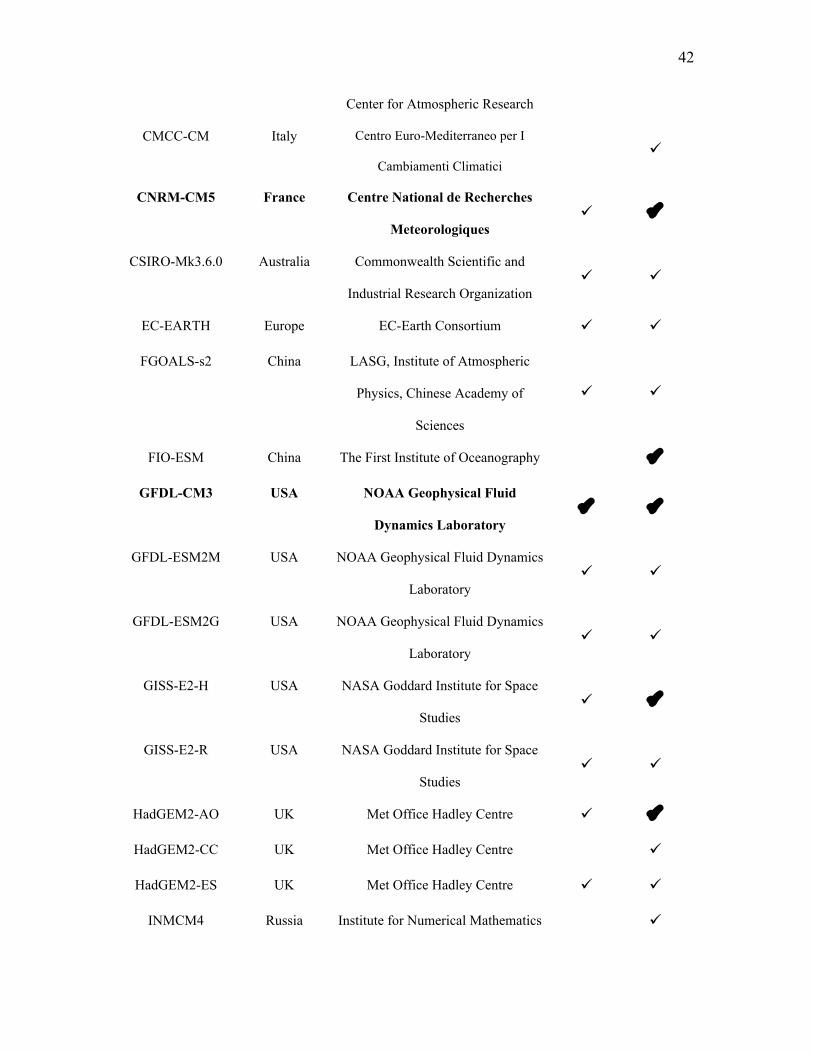
TABLE 1. Details of the WCRP CMIP5 global climate models used in this study. Check 882
marks indicate which scenarios are used. Five models were dynamically downscaled 883
(bold). All available models are statistically downscaled using the hybrid method. 884
885 MODEL COUNTRY INSTITUTE RCP2.6 RCP8.5
ACCESS1.0 Australia Commonwealth Scientific and
Industrial Research Organization
ACCESS1.3 Australia Commonwealth Scientific and
Industrial Research Organization
BCC-CSM1.1 China Beijing Climate Center, China
Meteorological Administration
BNU-ESM China College of Global Change and Earth
System Science, Beijing Normal
University
Can-ESM2 Canada Canadian Centre for Climate
Modelling and Analysis
CCSM4 USA National Center for Atmospheric
Research
CESM1(BGC) USA National Science Foundation,
Department of Energy, National
Center for Atmospheric Research
CESM1(CAM5) USA National Science Foundation,
Department of Energy, National
Center for Atmospheric Research
CESM1(WACCM) USA National Science Foundation,
Department of Energy, National
42
Center for Atmospheric Research
CMCC-CM Italy Centro Euro-Mediterraneo per I
Cambiamenti Climatici
CNRM-CM5 France Centre National de Recherches
Meteorologiques
CSIRO-Mk3.6.0 Australia Commonwealth Scientific and
Industrial Research Organization
EC-EARTH Europe EC-Earth Consortium
FGOALS-s2 China LASG, Institute of Atmospheric
Physics, Chinese Academy of
Sciences
FIO-ESM China The First Institute of Oceanography
GFDL-CM3 USA NOAA Geophysical Fluid
Dynamics Laboratory
GFDL-ESM2M USA NOAA Geophysical Fluid Dynamics
Laboratory
GFDL-ESM2G USA NOAA Geophysical Fluid Dynamics
Laboratory
GISS-E2-H USA NASA Goddard Institute for Space
Studies
GISS-E2-R USA NASA Goddard Institute for Space
Studies
HadGEM2-AO UK Met Office Hadley Centre
HadGEM2-CC UK Met Office Hadley Centre
HadGEM2-ES UK Met Office Hadley Centre
INMCM4 Russia Institute for Numerical Mathematics

43
IPSL-CM5A-LR France Institut Pierre Simon Laplace
IPSL-CM5A-MR France Institut Pierre Simon Laplace
MIROC-ESM Japan AORI (U. Tokyo), NIES,
JAMESTEC
MIROC-ESM-
CHEM
Japan AORI (U. Tokyo), NIES,
JAMESTEC
MIROC5 Japan AORI (U. Tokyo), NIES,
JAMESTEC
MPI-ESM-LR Germany Max Planck Institute for
Meteorology
MRI-CGCM3 Japan Meteorological Research Institute
NorESM1-M Norway Norwegian Climate Center
886 887 888
889
890
891
892
893
894
895
896
897
898
899

44
TABLE 2. Comparison of the spatial correlation and root mean squared error (RMSE) for 900
the raw GCM, linear interpolated and the statistically downscaled warming patterns, 901
relative to the dynamically downscaled warming. By virtue of their orthogonality, errors 902
in regional mean and spatial pattern are shown separately. 903
904
Annual Monthly Method
Spatial
Correlation
Spatial
RMSE
(°C)
Regional-
Mean
RMSE (°C)
Spatial
Correlation
Spatial
RMSE
(°C)
Regional-
Mean
RMSE
(°C)
Raw GCM 0.64 0.26 0.21 0.49 0.35 0.26
Linear
Interpolation
0.79 0.20 0.22 0.60 0.29 0.26
Statistical
Model
0.95 0.14 0.23 0.67 0.24 0.27
Note: Bolded values indicate improvements over linear interpolation. 905
906
907
908
909
910
911
912
45
(a)
−130 −125 −120 −115
30
35
40
(b)
−120 −119 −118 −11732.5
33
33.5
34
34.5
35
35.5
36
0 500 1000 1500 2000 2500 3000 913
914
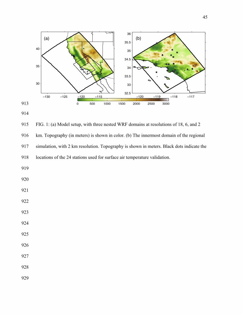
FIG. 1: (a) Model setup, with three nested WRF domains at resolutions of 18, 6, and 2 915
km. Topography (in meters) is shown in color. (b) The innermost domain of the regional 916
simulation, with 2 km resolution. Topography is shown in meters. Black dots indicate the 917
locations of the 24 stations used for surface air temperature validation. 918
919
920
921
922
923
924
925
926
927
928
929

46
5 10 15 20 25 305
10
15
20
25
30
r=0.72,Fallr=0.94,Winterr=0.82,Springr=0.93,Summer
point measurement (°C)
WRF
sim
ulat
ion
(°C)
(a) spatial variability
00.10.20.30.40.50.60.70.80.9
1
Baske
rsfiel
dBea
umon
tBurb
ank
Camari
lloEdw
ards
Fulle
rton
John
Way
neLa
ncas
ter
Long
Beach
Los A
lamito
s
Los A
ngele
sMoja
ve
Mounta
in Wilso
nOxn
ardPalm
dale
Point M
ugu
Riversi
de
San C
lemen
te
Santa
Barbara
Santa
Monica
Van N
uys
Buoy 4
6045
Buoy 4
6025
Sandb
urg
Corre
latio
n Co
effic
ient
(b) temporal variability
930
FIG. 2: Validation of WRF dynamical downscaling with against a network of 24 stations, 931
for the period 1995-2001. (a) Simulated versus observed seasonal average climatological 932
temperatures, for each of station. (b) Correlations at each station between the time series 933
of simulated and observed monthly temperature anomalies. Anomalies are relative to the 934
monthly climatology. 935
936
937
938
939
940
941
942
943
944
945
946

47
Jan Feb Mar Apr
May Jun Jul Aug
Sep Oct Nov Dec
Surface Air Warming (oC)0 1 2 3 4 5
947
FIG. 3: Monthly-mean surface air temperature change (°C) for the mid-century period 948
(2041-2060) relative to the baseline period (1981-2000) averaged over the five 949
dynamically downscaled GCMs. 950
951
952
953
954
955
956

48
EOF 1 EOF 2 EOF 3
957
FIG. 4: The spatial patterns associated with the three largest EOFs, in descending order of 958
size. EOF analysis was performed on the monthly warming patterns from the five 959
dynamically downscaled models, with the monthly domain averages removed. EOF 1 960
accounts for 74% of the variance. This EOF is referred to as the Coastal-Inland Pattern 961
(CIP) because of its negative loadings over the coastal land areas and positive loadings 962
inland. EOFs 2 and 3 account for 13% and 5% of the variance, respectively. 963
964
965
966
967
968
969
970
971
972
973

49
Coastal Inland Pattern (EOF 1)
−6 −4 −2 0 2 4 6(10−3 g kg−1)
Baseline Specific Humidity
11 10 9 8 7
974
FIG 5: Coastal-Inland Pattern (left) and surface specific humidity climatology (g kg-1) of 975
the baseline period (right). The two spatial patterns are highly correlated (r = -0.97). 976
977
978
979
980
981
982
983
984
985
986
987
988
989

50
−130 −125 −120 −115
28
30
32
34
36
38
40
42
44 (c)
Correlation Correlation Correlation
−130 −125 −120 −115
28
30
32
34
36
38
40
42
44 (a)
0.7 0.75 0.8 0.85 0.9 0.95 1
−130 −125 −120 −115
28
30
32
34
36
38
40
42
44 (b)
0 0.2 0.4 0.6 0.8 1 −0.5 0 0.5
990
FIG. 6: Correlations between GCM warming (interpolated to an 18-km grid) and the 991
dynamically downscaled (a) regional mean warming and (b) land-sea contrast in the 992
warming. The sampled regional mean warming and inland warming are calculated as 993
averages over the warming in the black boxes in panels (a) and (b), respectively. Panel 994
(c) shows partial correlations between the interpolated GCM warming and the 995
dynamically downscaled land-sea contrast with the effect of the sampled inland warming 996
removed. The ocean warming is calculated as the average over the black box in (c). 997
998
999
1000
1001
1002
1003
1004
1005
1006
1007

51
0 1 2 3 40
0.5
1
1.5
2
2.5
3
3.5
4
4.5
GCM Sampled (oC)
Dyna
mica
lly D
owns
cale
d (o C)
Regional Mean Warming
r = 0.95
CCSM4GFDL−CM3MIROC−ESM−CHEMCNRM−CM5MPI−ESM−LR
−1 0 1 2 3−1
−0.5
0
0.5
1
1.5
2
2.5
3
GCM Sampled (oC)
Dyna
mica
lly D
owns
cale
d (o C)
Land−Sea Contrast
r = 0.79
1008
FIG. 7: Scatter plots of dynamically downscaled regional mean warming versus GCM-1009
sampled regional mean warming (left), and dynamically downscaled land-sea contrast 1010
versus the GCM-sampled land-sea contrast (right). For each GCM (colors), the twelve 1011
monthly-mean warming values are shown. Approximations used by the statistical model 1012
are shown as black dashed lines. 1013
1014
1015
1016
1017
1018
1019
1020
1021
1022
1023
1024
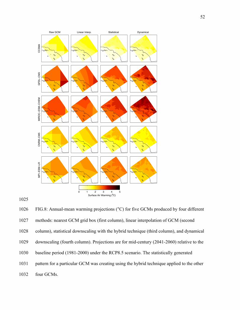
52
Dynamical Statistical Linear Interp. Raw GCM
CCSM
4G
FDL−
CM3
MIR
OC−
ESM−C
HEM
CNRM
−CM
5M
PI−E
SM−L
R
Surface Air Warming (oC)
0 1 2 3 4 5
1025
FIG.8: Annual-mean warming projections (°C) for five GCMs produced by four different 1026
methods: nearest GCM grid box (first column), linear interpolation of GCM (second 1027
column), statistical downscaling with the hybrid technique (third column), and dynamical 1028
downscaling (fourth column). Projections are for mid-century (2041-2060) relative to the 1029
baseline period (1981-2000) under the RCP8.5 scenario. The statistically generated 1030
pattern for a particular GCM was creating using the hybrid technique applied to the other 1031
four GCMs. 1032

53
oC
−1
−0.5
0
0.5
1
oC
0
1
2
3
4
5(a) Raw GCM (b) Linear Interp. (c) Statistical (d) Dynamical
(e) Raw GCM (f) Linear Interp. (g) Statistical
1033
FIG. 9: Annual-mean warming (°C) averaged over five GCMs downscaled using four 1034
different methods: (a) nearest GCM grid box, (b) linear interpolation of GCM, (c) 1035
statistical downscaling with hybrid technique, (d) dynamical downscaling. Bias of first 1036
three methods relative to dynamical downscaling (°C) shown in (e)-(g). 1037
1038
1039
1040
1041
1042
1043
1044
1045
1046
1047
1048

54
0 0.5 1 1.5 2 2.5 3 3.5 40
0.5
1
1.5
GFDL−ESM2M
GFDL−ESM2G
GFDL−CM3
CNRM−CM5
CanESM2
GISS−E2−R
HadGEM2−CC
HadGEM2−ES
IPSL−CM5A−LR
IPSL−CM5A−MR
MIROC−ESM−CHEM
MIROC−ESMMIROC5
MPI−ESM−LRMRI−CGCM3
NorESM1−M
INM−CM4
ACCESS1.0
ACCESS1.3
BNU−ESM
CESM1(BGC)
CESM1(CAM5)
CESM1(WACCM)
CMCC−CM
CSIRO−Mk3.6.0
EC−EARTH
FGOALS−s2
FIO−ESM
GISS−E2−H HadGEM2−AO
BCC−CSM1.1
CCSM4
Ensemble Mean
Regional Mean Warming (oC)
Land−S
ea C
ontra
st (o C)
1049
FIG.10: Annual-mean values of regional-mean warming and land-sea contrast (°C) for 1050
each GCM (blue dots) with the ensemble mean (red dot). The five GCMs that are also 1051
dynamically downscaled are highlighted in green. 1052
1053
1054
1055
1056
1057
1058
1059
1060

55
ACCESS1.0 ACCESS1.3 BCC−CSM1.1 BNU−ESM CanESM2 CCSM4 CESM1(BGC) CESM1(CAM5)
CESM1(WACCM) CMCC−CM CNRM−CM5 CSIRO−Mk3.6.0 EC−EARTH FGOALS−s2 FIO−ESM GFDL−CM3
GFDL−ESM2G GFDL−ESM2M GISS−E2−H GISS−E2−R HadGEM2−AO HadGEM2−CC HadGEM2−ES INM−CM4
IPSL−CM5A−LR IPSL−CM5A−MR MIROC−ESM MIROC−ESM−CHEM MIROC5 MPI−ESM−LR MRI−CGCM3 NorESM1−M
Surface Air Warming (oC)
0 0.5 1 1.5 2 2.5 3 3.5 4 4.5
1061
FIG. 11: Annual-mean warming patterns (°C) generated by applying the statistical model 1062
to all 32 GCMs. Warming patterns are shown for the mid-century period (2041-2060) 1063
relative to the baseline period(1981-2000), under the RCP8.5 scenario. 1064
1065
1066
1067
1068
1069
1070
1071
1072
1073
1074
1075

56
Lower Bound Ensemble Mean
Surface Air Warming (oC)
Upper Bound
0 1 2 3 4 5
1076
FIG.12: Ensemble-mean annual-mean warming and upper and lower bounds (°C), based 1077
on a 95% confidence interval, for 32 statistically downscaled GCMs run with the RCP8.5 1078
scenario. 1079
1080
1081
1082
1083
1084
1085
1086
1087
1088
1089
1090
1091
1092

57
Jan Feb Mar Apr
May Jun Jul Aug
Sep Oct Nov Dec
Surface Air Warming (oC)
0 1 2 3 4 5
1093
FIG.13: Ensemble-mean monthly-mean warming (°C) computed by averaging the 1094
monthly statistically downscaled warming patterns over 32 CMIP5 GCMs. 1095