Embed Size (px)
Citation preview
Preface
Return to Basics (RTB) is a project to re-create a modern interpretation of the BASICinterpreter and programming environment popular in the late 1970s through the 1980son the popular 8-bit microprocessor systems such as the Apple // series, BBC Micro,Commodore PET, Tandy TRS-80, as well as the various Sinclair systems and a wholehost of others too numerous to mention. The intention is to present an easy to useenvironment for young (and old) people to learn to write computer programs using aninteractive system that’s quick and easy to use.
BASIC (Beginners All-purpose Symbolic Instruction Code) first demonstrated 50years ago1, is regarded as somewhat old-fashioned in todays world but I believe itstill has a place in the teaching and learning of computer programming. It arguablyhas many faults and has been criticised for encouraging bad programming practices2,however RTB is a new implementation, capable of using modern structured programingtechniques including named functions and procedures (which support local variablesand recursion, if desired) and structured looping constructs, making line numbers andGOTO completely optional.
Today, BASIC is still used in commercial applications, but not in the traditional form– it exists in the form of Microsoft VB and VB.NET and many derivatives.
RTB is not intended to be used as a serious programming system – While it hasthe capabilities to write a large financial or scientific package in, I do not expect peopleto write the many, varied and large packages that were commonly written in BASIC inthose early days, but rather to be used as a way to introduce programming in an easyto understand manner, then allow those who have the aptitude and skill to go on tolearning other modern programming languages.
RTB features several graphical systems that were popular in those early micropro-cessor years – both a low and high resolution colour graphics system as well as “turtle”graphics with simplified colour and angle handling. Sprites and sounds are supportedtoo and it is more than capable of being used to write games and animations in.
I would like to think that pre-teen children can be introduced to programming usingRTB – the only prerequisite is a desire to learn and the ability to type some simpleinstructions into a computer. It doesn’t even need a mouse! (Although you can enablemouse use in your own programs)
This book is intended to be used as a reference manual for RTB. It lists all the majorprogramming constructs with a small number of examples.
Gordon Henderson, Last updated: June 2014
11st May, 1964, Dartmouth College, MA, USA2BASIC doesn’t teach bad programming, bad teachers do
i

Trademarks and Acknowledgements
• Raspberry Pi is a registered trademark of the Raspberry Pi Foundation.
• ”Minecraft” is a trademark of Notch Development AB.
• All other trademarks, etc. are acknowledged.
ii
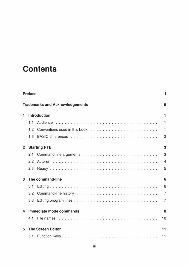
Contents
Preface i
Trademarks and Acknowledgements ii
1 Introduction 1
1.1 Audience . . . . . . . . . . . . . . . . . . . . . . . . . . . . . . . . . . . 1
1.2 Conventions used in this book . . . . . . . . . . . . . . . . . . . . . . . . 1
1.3 BASIC differences . . . . . . . . . . . . . . . . . . . . . . . . . . . . . . 2
2 Starting RTB 3
2.1 Command line arguments . . . . . . . . . . . . . . . . . . . . . . . . . . 3
2.2 Autorun . . . . . . . . . . . . . . . . . . . . . . . . . . . . . . . . . . . . 4
2.3 Ready . . . . . . . . . . . . . . . . . . . . . . . . . . . . . . . . . . . . . 5
3 The command-line 6
3.1 Editing . . . . . . . . . . . . . . . . . . . . . . . . . . . . . . . . . . . . . 6
3.2 Command-line history . . . . . . . . . . . . . . . . . . . . . . . . . . . . 7
3.3 Editing program lines . . . . . . . . . . . . . . . . . . . . . . . . . . . . . 7
4 Immediate mode commands 8
4.1 File names . . . . . . . . . . . . . . . . . . . . . . . . . . . . . . . . . . 10
5 The Screen Editor 11
5.1 Function Keys . . . . . . . . . . . . . . . . . . . . . . . . . . . . . . . . . 11
iii

5.2 Control Keys . . . . . . . . . . . . . . . . . . . . . . . . . . . . . . . . . 12
5.3 A guide on usage . . . . . . . . . . . . . . . . . . . . . . . . . . . . . . . 13
5.4 Syntax highlighting . . . . . . . . . . . . . . . . . . . . . . . . . . . . . . 14
6 Introduction to RTB programming 16
6.1 What an RTB program looks like . . . . . . . . . . . . . . . . . . . . . . 17
7 Comments 18
8 Variables 19
8.1 Names . . . . . . . . . . . . . . . . . . . . . . . . . . . . . . . . . . . . . 19
8.2 Types . . . . . . . . . . . . . . . . . . . . . . . . . . . . . . . . . . . . . 19
8.3 Assignment . . . . . . . . . . . . . . . . . . . . . . . . . . . . . . . . . . 20
8.4 Numeric operators and Precedence . . . . . . . . . . . . . . . . . . . . 20
8.5 String Operators . . . . . . . . . . . . . . . . . . . . . . . . . . . . . . . 20
8.6 Arrays . . . . . . . . . . . . . . . . . . . . . . . . . . . . . . . . . . . . . 21
8.7 Associative Arrays . . . . . . . . . . . . . . . . . . . . . . . . . . . . . . 21
9 Flow Control 22
9.1 GOTO and GOSUB – The great controversy . . . . . . . . . . . . . . . . 23
9.2 Line numbers or No line numbers? . . . . . . . . . . . . . . . . . . . . . 24
10 Text and Number Input 25
11 Text and Number Output 29
11.1 updateMode . . . . . . . . . . . . . . . . . . . . . . . . . . . . . . . . . 29
11.2 Variables affecting output . . . . . . . . . . . . . . . . . . . . . . . . . . 31
12 Conditionals: IF . . . THEN . . . 32
12.1 Multiple lines . . . . . . . . . . . . . . . . . . . . . . . . . . . . . . . . . 32
12.2 IF . . . THEN . . . ELSE . . . ENDIF . . . . . . . . . . . . . . . . . . . . . . . 33
iv

13 Conditionals: SWITCH and CASE. . . 35
14 Looping the Loop 38
14.1 CYCLE . . . REPEAT . . . . . . . . . . . . . . . . . . . . . . . . . . . . . 38
14.1.1 UNTIL . . . . . . . . . . . . . . . . . . . . . . . . . . . . . . . . . 39
14.1.2 WHILE . . . . . . . . . . . . . . . . . . . . . . . . . . . . . . . . 39
14.2 For Loops . . . . . . . . . . . . . . . . . . . . . . . . . . . . . . . . . . . 40
14.3 Breaking and continuing the loop . . . . . . . . . . . . . . . . . . . . . . 41
15 Data, Read and Restore 42
16 Miscellaneous Program instructions 45
17 Numerical Functions and data 46
17.1 System variables and constants . . . . . . . . . . . . . . . . . . . . . . . 46
17.2 Functions . . . . . . . . . . . . . . . . . . . . . . . . . . . . . . . . . . . 47
18 String Functions and data 49
18.1 System variables . . . . . . . . . . . . . . . . . . . . . . . . . . . . . . . 49
18.2 Functions . . . . . . . . . . . . . . . . . . . . . . . . . . . . . . . . . . . 49
19 Graphics 51
19.1 System Variables . . . . . . . . . . . . . . . . . . . . . . . . . . . . . . . 51
19.2 General Graphics . . . . . . . . . . . . . . . . . . . . . . . . . . . . . . . 52
19.3 Cartesian Graphics . . . . . . . . . . . . . . . . . . . . . . . . . . . . . . 54
19.4 Turtle Graphics . . . . . . . . . . . . . . . . . . . . . . . . . . . . . . . . 55
19.5 Sprites . . . . . . . . . . . . . . . . . . . . . . . . . . . . . . . . . . . . . 55
20 Mouse Input 58
21 Sound 59
21.1 Music . . . . . . . . . . . . . . . . . . . . . . . . . . . . . . . . . . . . . 59
v
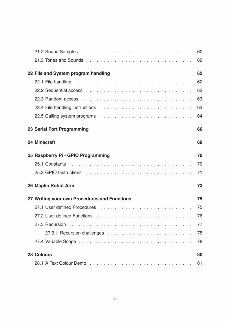
21.2 Sound Samples . . . . . . . . . . . . . . . . . . . . . . . . . . . . . . . . 60
21.3 Tones and Sounds . . . . . . . . . . . . . . . . . . . . . . . . . . . . . . 60
22 File and System program handling 62
22.1 File handling . . . . . . . . . . . . . . . . . . . . . . . . . . . . . . . . . 62
22.2 Sequential access . . . . . . . . . . . . . . . . . . . . . . . . . . . . . . 62
22.3 Random access . . . . . . . . . . . . . . . . . . . . . . . . . . . . . . . 63
22.4 File handling instructions . . . . . . . . . . . . . . . . . . . . . . . . . . 63
22.5 Calling system programs . . . . . . . . . . . . . . . . . . . . . . . . . . 64
23 Serial Port Programming 66
24 Minecraft 68
25 Raspberry Pi - GPIO Programming 70
25.1 Constants . . . . . . . . . . . . . . . . . . . . . . . . . . . . . . . . . . . 70
25.2 GPIO Instructions . . . . . . . . . . . . . . . . . . . . . . . . . . . . . . 71
26 Maplin Robot Arm 73
27 Writing your own Procedures and Functions 75
27.1 User defined Procedures . . . . . . . . . . . . . . . . . . . . . . . . . . 75
27.2 User defined Functions . . . . . . . . . . . . . . . . . . . . . . . . . . . 76
27.3 Recursion . . . . . . . . . . . . . . . . . . . . . . . . . . . . . . . . . . . 77
27.3.1 Recursion challenges . . . . . . . . . . . . . . . . . . . . . . . . 78
27.4 Variable Scope . . . . . . . . . . . . . . . . . . . . . . . . . . . . . . . . 78
28 Colours 80
28.1 A Text Colour Demo . . . . . . . . . . . . . . . . . . . . . . . . . . . . . 81
vi

Chapter 1
Introduction
1.1 Audience
This book is aimed at people who may already have a familiarity with BASIC or otherhigh-level languages. It’s mainly a reference book for the language, but that are a fewexamples along the way to help emphasise some of the concepts and features beingdescribed.
It is assumes that you understand the basic principles of computing and know con-cepts like volatile and non-volatile storage and so on and how to type simple commandsinto your (Linux) computer.
The examples will make reference to RTB keywords, commands and functions thatmay not have been covered up to that point - use the rest of this book as a referencemanual and consult the index - it’s really not intended to be read from start to finish inthat order.
1.2 Conventions used in this book
Keeping things simple is the aim here, so there are only really 3 things to look outfor1. The first is that anything you may need to type into a computer running RTB, oranything it prints will be in this typewriter style font. The second is that anything ofsome importance, such as a name of an algorithm is emphasised like this.
The final thing to look out for is a warning, or just something that may be important!
1OK, Possibly four as there may be the occasional footnote at the bottom of a page, so look out forthem too.
1

CHAPTER 1. INTRODUCTION 2
to remember. It’s represented by a warning exclamation point in a box to the side ofthe text. As demonstrated in this paragraph.
1.3 BASIC differences
If you know what you’re doing, here are some brief differences between RTB and a“classic” BASIC:
• RTB does not allow multiple statements on one line; One statement per line only.
• Items to be printed using the PRINT command must be separated by a semicolon(;) and no additional spacing is added. See the numformat command for detailson formatting numbers.
• Variable names can be of almost any length and upper/lower case is significant.
• IF statements must have THEN (So no IF... num = 4, or IF... GOTO 10, it mustbe the full IF... THEN GOTO 10, or IF... THEN a = 7, etc.)
• In FOR loops, there is no NEXT instruction – it’s replaced by the CYCLE...REPEAT
construct.
• Named procedures and functions. (Which can be called recursively)
• Local variables inside user-defined procedures and functions.
• A single looping construct (CYCLE...REPEAT) which can be modified with FOR,WHILE and UNTIL constructs.
• BREAK and CONTINUE as part of the looping construct.
• Arrays start at zero and go up to and include the number in the DIM statement. ie.the DIM statement specifies the size of the array plus one.
Additionally (where supported) the graphical systems may well be new or differentto you. RTB incorporates simple block/line graphics as well as turtle graphics using avariety of angle modes (degrees, radians and clock).

Chapter 2
Starting RTB
RTB is primarily designed to run on computers running Linux. In the fullness of time,both MS windows and Apple Mac versions may be made available, but for now it’sLinux only.
On the Raspberry Pi, there are some additional features to make use of the Pi’sGPIO facility.
Starting RTB may vary from one Linux system another, however opening up a text(or command/shell) terminal and typing
rtb
at the prompt will usually get things going for you. You may have a desktop iconwhich you can click on too.
RTB runs equally well under X windows on directly on the console.
Whatever the system, once RTB has started it should look the same. There willbe a keyboard to type commands into, this is connected to the main computer whichshould be connected to a screen or display of some sort. A Raspberry Pi may even beconnected to your home TV set. The mouse is not normally needed, but may be usedin the editor and by your own program.
2.1 Command line arguments
RTB can take additional arguments (parameters) on the command-line. The usage lineis:
Usage: rtb [-s] [-f] [-d] [-H] [-m mode] [-x xSize] [-y ySize] [-z bpp]
3
CHAPTER 2. STARTING RTB 4
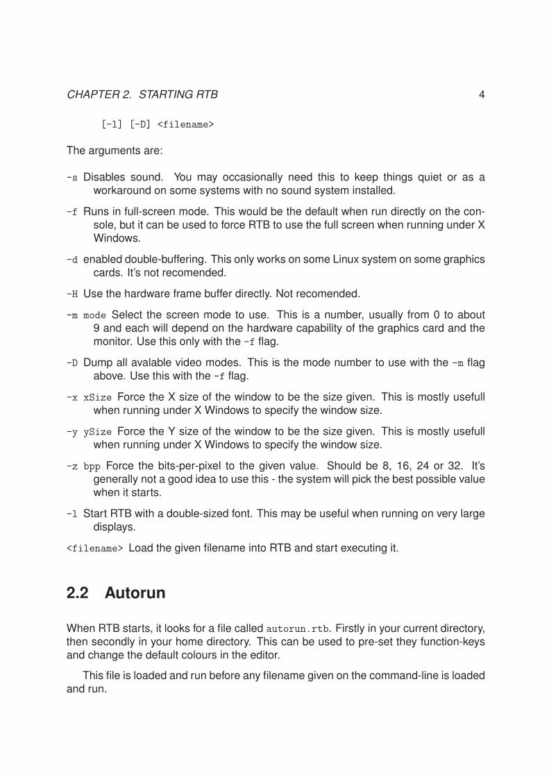
[-l] [-D] <filename>
The arguments are:
-s Disables sound. You may occasionally need this to keep things quiet or as aworkaround on some systems with no sound system installed.
-f Runs in full-screen mode. This would be the default when run directly on the con-sole, but it can be used to force RTB to use the full screen when running under XWindows.
-d enabled double-buffering. This only works on some Linux system on some graphicscards. It’s not recomended.
-H Use the hardware frame buffer directly. Not recomended.
-m mode Select the screen mode to use. This is a number, usually from 0 to about9 and each will depend on the hardware capability of the graphics card and themonitor. Use this only with the -f flag.
-D Dump all avalable video modes. This is the mode number to use with the -m flagabove. Use this with the -f flag.
-x xSize Force the X size of the window to be the size given. This is mostly usefullwhen running under X Windows to specify the window size.
-y ySize Force the Y size of the window to be the size given. This is mostly usefullwhen running under X Windows to specify the window size.
-z bpp Force the bits-per-pixel to the given value. Should be 8, 16, 24 or 32. It’sgenerally not a good idea to use this - the system will pick the best possible valuewhen it starts.
-l Start RTB with a double-sized font. This may be useful when running on very largedisplays.
<filename> Load the given filename into RTB and start executing it.
2.2 Autorun
When RTB starts, it looks for a file called autorun.rtb. Firstly in your current directory,then secondly in your home directory. This can be used to pre-set they function-keysand change the default colours in the editor.
This file is loaded and run before any filename given on the command-line is loadedand run.

CHAPTER 2. STARTING RTB 5
2.3 Ready
When it’s setup and ready, the screen should be clear apart from a logo, some intro-ductory text and a prompt. It will probably look something like this:
Ready
>
The “>” symbol is the prompt. It’s presence means that RTB is ready to accept com-mands and program lines typed into it.

Chapter 3
The command-line
The command line is the general term for typing commands and program lines into thesystem, however it has a few features to make your life easier.
Note that it is possible to develop and run RTB programs without ever using thecommand line! You can press F2 as soon as the system has started to use the full-screen editor, then run your program from there. However, the commands you canenter in immediate mode may allow you to test parts of your program, examine thefile-system and so on.
3.1 Editing
As you type characters into the system, you may make mistakes. To correct themyou can use several different keys. The important one is probably the Backspace key.Usually a big key to the top-right of the main keyboard with an arrow pointing to the left.This will erase characters you’ve typed and move the cursor to the left, however thereare more efficient ways to deal with the line you’re typing noted below.
Some of the command characters listed below you access with the Control key.This is labelled as Ctrl on most keyboards and works like the Shift keys in that youpush it, keep it pushed, then type another character before releasing them both.
Ctrl-A, Ctrl-E: Move the cursor to the start or the end of the line respectively. Youcan also use the Home and End keys if your keyboard has them.
← (Left) and→ (Right): arrow keys (not to be confused with the Backspace key)move the cursor one character to the left or right of the typed line.
6

CHAPTER 3. THE COMMAND-LINE 7
Ctrl-D: Delete the character under the cursor. You can also use the Del or Delete keyif your keyboard has one.
Backspace: Deletes the character to the Left of the cursor)
Ctrl-S: Swap the character under the cursor with the character immediately to theright. Handy for those who type the as teh like me. . .
Ctrl-F: Find the next occurrence of the next character typed. E.g. Ctrl-F followed byG will make the cursor jump to the next G in the line. Ctrl-F followed by anotherCtrl-F will repeat the last find.
Esc: Abandon entering this entire line.
3.2 Command-line history
The RTB command line remembers the past 50 lines that you type in, and you can usethe ↑ (Up) and ↓ (Down) arrow keys on your keyboard to scroll through past things you’vetyped in. This will enable you to quickly fix a mistake in a line already in the system, ora line you typed in which reported an error after you pressed the Enter key.
3.3 Editing program lines
If you spot a mistake in a program line and you can’t find it in the history, then you canenter the ED command followed by the line number. E.g. ED 10 will then present line10 as if you had re-typed it, but not yet pressed Enter so you can change the line asrequired.

Chapter 4
Immediate mode commands
In immediate mode, as well as executing simple print instructions and other instructionsyou can use within a program, there are several commands which can only be executedin immediate mode.
Commands may be typed in in upper or lower case. Some commands are pre-sented below in mixed case - this is just to make it easier to see what the commandis.
list [[first] last]: This lists the program stored in memory to the screen. You canpause the listing with the space-bar and terminate it with the escape key. If firstis given, then only that line will be listed. If both first and last are given, thenlines in that range will be listed.
save [filename]: Saves your program to the local storage medium. filename is thename of the file you wish to save as. If you want to include spaces in the filename,then you need to enclose the name inside double-quotes. If you have alreadysaved a file, then you can subsequently execute SAVE without the filename and itwill overwrite the last file saved. (This is “safe” as it’s reset when you load a newprogram or use the NEW command)
Note that the program is saved without line-numbers, even if you used line num-!bers to enter the program in interactive mode. If your program contains refer-ences to line numbers (e.g. GOTO, GOSUB or RESTORE commands) then you will beprompted to use the saveN command below.
saveN [filename]: Same as the normal save command, but saves with your line num-bers included.
load filename: Loads in a program from the local storage. As with save, you need touse double-quotes if the filename contains spaces.
8

CHAPTER 4. IMMEDIATE MODE COMMANDS 9
ls [directory]: Lists the RTB files and directories in your current working directory,or the given directory (as above, use double-quotes to select directories withspaces in them)
dir [directory]: An alias for ls above.
cd [directory]: Changes directory to the one given. If no directory is given, then itchanges to your “home” directory.
pwd: Prints your current Working Directory.
new: Deletes the program in memory. There is no “Are you sure?” verification andonce it’s gone, it’s gone. Remember to save first!
run: Runs the program in memory. You may give a line number and the program willstart from that number rather than the first line in the program. Note that usingrun will clear all variables.
cont: Continues program execution after a STOP instruction. Variables are not cleared.
resume: An alias for the cont command.
clear: Clears all variables and deletes all arrays. It also removes any active spritesfrom the screen and stops all sounds playing. Stopped programs may not becontinued after a clear command.
tron: Trace-On: Turns line-number tracing on. As each line is executed, it’s number isprinted to the text console that RTB was started from - you may need to run yourprogram in a smaller window than full-screen to see the trace.
troff: Trace-Off: Turns line number tracing off.
ed linenumber: Edit the line given.
edit: Edits the current program in the full-screen editor.
renumber [start [inc [first [last]]]]: This renumbers your program - by defaultit will start at 100 and go in increments of 10, however you can change this asfollows: The start and inc parameters specify the new starting line number andincrement, the first and last parameters specify the first and last exiting linenumbers to renumber. Using this latter way, you can move lines in the program,but beware of overlaps.
If an overlap does occur, then renumbering will stop at that point and you mayfind your program to be somewhat scrambled. . . Please make sure you save yourprogram before renumbering!
version: Print the current version of RTB.
CHAPTER 4. IMMEDIATE MODE COMMANDS 10
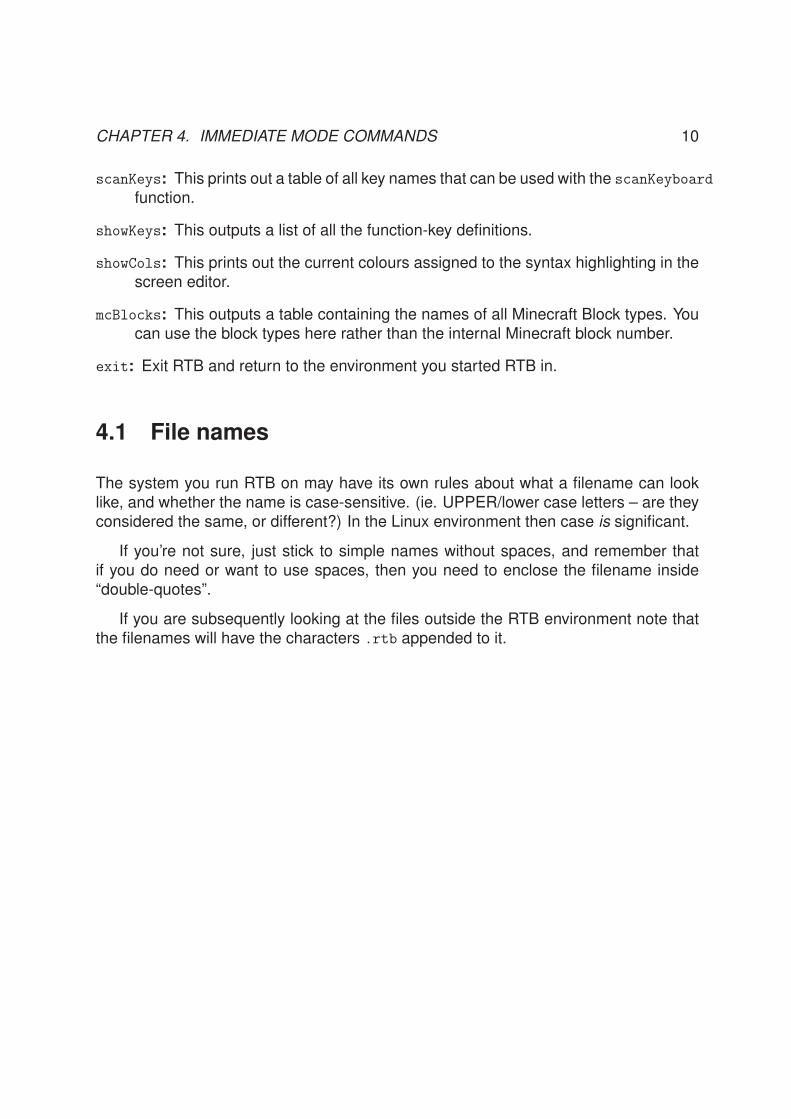
scanKeys: This prints out a table of all key names that can be used with the scanKeyboard
function.
showKeys: This outputs a list of all the function-key definitions.
showCols: This prints out the current colours assigned to the syntax highlighting in thescreen editor.
mcBlocks: This outputs a table containing the names of all Minecraft Block types. Youcan use the block types here rather than the internal Minecraft block number.
exit: Exit RTB and return to the environment you started RTB in.
4.1 File names
The system you run RTB on may have its own rules about what a filename can looklike, and whether the name is case-sensitive. (ie. UPPER/lower case letters – are theyconsidered the same, or different?) In the Linux environment then case is significant.
If you’re not sure, just stick to simple names without spaces, and remember thatif you do need or want to use spaces, then you need to enclose the filename inside“double-quotes”.
If you are subsequently looking at the files outside the RTB environment note thatthe filenames will have the characters .rtb appended to it.

Chapter 5
The Screen Editor
To help you develop and edit programs, especially when you do not wish to use oldstyle line numbers, RTB incorporates a simple full-screen editor with optional syntaxhighlighting.
To access the editor, just use the EDIT command, or press the F3 key which defaultsto EDIT unless you’ve re-defined it.
The editor will read in the last file you loaded or saved. If you have changed thecurrent program in the interactive environment, then you will be asked to SAVE (or NEWbefore editing it. If you have not loaded or saved and programs so-far, it will start withan empty file and you’ll be asked to save it before returning to the interpreter.
The screen editor shares some of the control-key commands as the line editor, butalso introduces more of its own as well as a set of function keys.
There is no mode to the editor - anything you type is inserted into your program.To command the editor, you use control characters and the Function keys. If you areused to some Linux or MS editors, it is more like “nano”, or “notepad” than “vim” in thatrespect.
Some of the command characters listed below you access with the Control key.This is labelled as Ctrl on most keyboards and works like the Shift keys in that youpush it, keep it pushed, then type another character before releasing them both.
5.1 Function Keys
ESC: Abandon editing the entire file. (You are prompted if you have changed anythingfirst)
11

CHAPTER 5. THE SCREEN EDITOR 12
F1: Pressing the F1 key will bring up a quick-help page, should you forget some of thecommands.
F2: This saves your file and loads it into the interpreter. If there are any load errors,you are promoted to return to the editor with the cursor positioned on the line inerror.
F3: As above (F2) but also attempts to run the program. If there are any errors, youare prompted to return to the editor, or stay in the interactive environment ( whichmay be handy for debugging, printing variables, and so on)
F4: Toggles syntax highlighting on or off.
F5: Saves your work. A save is performed automatically when you exit the editor, butthis allows you to save at any time. (May be handy if you are expecting a powercut)
F8: Loads a new file into the editor. If you have changed the current file, you areprompted to save it first.
F9: Discards all edits and reverts to the last saved version of your file.
F10: Inserts a file at the current cursor location. This can allow you to build up librariesof procedures and functions.
F12: Erase the current file. This deletes the file from memory and resets the filename- it doesn’t change any file on disk unless you subsequently save with the samefilename.
5.2 Control Keys
Ctrl-O: This will open a new line for text entry over the current line. Handy if you’re onthe top line and want to add text above it.
Ctrl-M: This will open a new line for text entry under the current line. Normally to entera new line, you would move to the end of the line then press enter. This is just ashort cut.
Ctrl-A, Ctrl-E: Move the cursor to the start or the end of the line respectively. Youcan also use the Home and End keys if your keyboard has them.
← (Left) and→ (Right): arrow keys (not to be confused with the Backspace key)move the cursor one character to the left or right of the typed line.

CHAPTER 5. THE SCREEN EDITOR 13
↑ (Up) and ↓ (Down): arrow keys move the cursor one character up or down from thecurrent line.
Page Up, Page Down: Move the cursor one page up or down.
Ctrl-Z: Centres the cursor on the page. This will move the screen up or down to makethe line the cursor is currently on in the middle of the screen.
Ctrl-D: Delete the character under the cursor. You can also use the Del or Delete keyif your keyboard has one.
Backspace: Deletes the character to the Left of the cursor. (This is the key that’s nor-mally above the Enter key.
Ctrl-S: Swap the character under the cursor with the character immediately to theright. Handy for those who type the as teh like me. . .
Ctrl-F: Find the next occurrence of the next character typed on the current line. E.g.Ctrl-F followed by G will make the cursor jump to the next G in the line. Ctrl-F fol-lowed by another Ctrl-F will repeat the last find. The search is case-insensitive.
Ctrl-K or Ctrl-X: Kill the current line - this deletes the from the screen and copies itinto the paste buffer. You can use Ctrl-K several times to delete multiple linesand move them to the paste buffer, however if you move the cursor, then kill morelines, the first batch of lines will be lost!
Ctrl-U: Un-kill Under: This copies all lines in the paste buffer under the current line.
Ctrl-V: Un-kill oVer: This copies all lines in the paste buffer oVer the current line.
Ctrl-W: Where Is: This is the word search facility. You are prompted for some textto search for and the editor will search through to try to find it. The search iscase-insensitive.
Ctrl-J: Jump to a line number. You are prompted for the line number to jump to.
Ctrl-G: Prints the current line number. Note that this is the line number inside the file,and is not the same as the line numbers which may be used to enter programs ininteractive mode.
5.3 A guide on usage
In-general the cursor can be moved by the arrow keys and the Page Up/Down keys.You can also use the mouse scroll wheel to move up and down, or click the mouse onany character to move the cursor directly there. Ctrl-Z will move the current line to the
CHAPTER 5. THE SCREEN EDITOR 14
middle of the screen which might make it easier to see more lines above or below theone you’re working on.
You should be able to do all editing without using the mouse at all - it’s far moreefficient to keep your hands on the keyboard than to constantly move one over to themouse and back again.
Copy and paste is accomplished using the Ctrl-K (to Kill lines) and Ctrl-U - toUn-Kill lines. To move a block of text, you would position the cursor on the first line inthe block, then press Ctrl-K as many times as needed – noting that this will delete thelines. If you’re copying the block, then you can immediately press Ctrl-U - which pastesthe deleted lines back where they were, then move the cursor and press Ctrl-U again.You can paste as many times as you need to to repeat the lines, if required.
5.4 Syntax highlighting
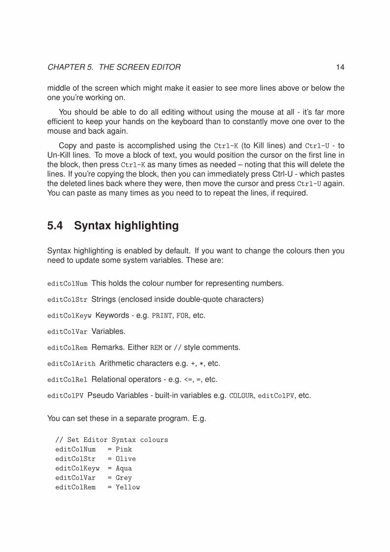
Syntax highlighting is enabled by default. If you want to change the colours then youneed to update some system variables. These are:
editColNum This holds the colour number for representing numbers.
editColStr Strings (enclosed inside double-quote characters)
editColKeyw Keywords - e.g. PRINT, FOR, etc.
editColVar Variables.
editColRem Remarks. Either REM or // style comments.
editColArith Arithmetic characters e.g. +, *, etc.
editColRel Relational operators - e.g. <=, =, etc.
editColPV Pseudo Variables - built-in variables e.g. COLOUR, editColPV, etc.
You can set these in a separate program. E.g.
// Set Editor Syntax colours
editColNum = Pink
editColStr = Olive
editColKeyw = Aqua
editColVar = Grey
editColRem = Yellow

CHAPTER 5. THE SCREEN EDITOR 15
editColArith = Silver
editColRel = Red
editColSysV = Green
end
You may wish to investigate the autorun.rtb program too. This is a program that’sautomatically loaded and run each time you start RTB.
Chapter 6
Introduction to RTB programming
RTB programs are essentially a list of instructions for the computer to follow, one in-struction per line.
The syntax follows an easy to read system, designed to make it easy to both entera new program and understand an existing one.
The structure of your program, indentation, upper/lower case, etc. is entirely up toyou. Nothing is enforced by the system, although if you use the LIST command, thenyou will get an idea of what the program looks like to the computer as it will interpretyour program in the way it executes it.
Using the LIST command is handy from time to time too, as it will highlight potentialplaces where you may have forgotten to use an ENDIF, or missing REPEAT from a CYCLE
instruction.
Here is a quick guide to entering and running a program.
Start RTB. At the > prompt, press F2 to enter the editor, and type the following intothe editor:
print "Hello world"
end
Pressing F3 will save then run your program. Enter a filename - e.g. test (no needto add .rtb to it) then your program will be saved and run.
You can then return to the editor, or press ESC to return to immediate mode whereyou can use the RUN command to re-run your program.
16

CHAPTER 6. INTRODUCTION TO RTB PROGRAMMING 17
6.1 What an RTB program looks like
The example above is the simplest RTB program. Programs can be entered in upper orlower case, although if you LIST the program you’ll note that some keywords have beenchanged, as well as the program spacing. This is how RTB sees the program internally- as long as you use the screen editor, you can maintain your program format, style,etc. as you wish. There is no need to use spacing or indentation although it can helpmake your programs more readable (and I strongly recommend you do space yourprograms out and indent sections inside loops, etc.) You can use upper case or lowercase as you desire. My own preference is to use a form of “Camel Caps” but start witha lower-case letter. e.g. numberOfCows
Programs don’t need to start with anything special - jump right in, but a few comment-lines are handy. Programs should also end with the END statement - this can be any-where. It performs a graceful exit to the program. You can also use the STOP keywordtoo - then it will print a message and stop running. At this point, you can examinevariables, etc. then, if-required use the CONT command to contine program execution.STOP and CONT are really intended as program debugging aids.
A sample program to give you more idea:
// Many Hello Worlds
cls
for lines = 1 to 10 cycle
proc indent (lines)
print "Hello, world"
repeat
end
// proc indent:
// Output some dots (see also the space$() function)
def proc indent (distance)
local count
for count = 1 to distance cycle
print ".";
repeat
endproc

Chapter 7
Comments
It’s always a good idea to include comments in your programs, and RTB provides 2methods to help you do this.
Firstly, there is the traditional BASIC REM statement. Short for “Remark”. Secondlythere is the // statement which is common in many other programming languages.
REM must appear at the start of a program line, but // may appear anywhere in aline - and anything after the // is ignored.
Examples:
REM This is a demonstration of comments
//
REM // on its own can be used to separate program sections.
//
// But blank lines are also allowed when you use the screen editor
// but appear as empty // lines in the LIST output.
// The line below is allowed:
LET test = 42 // Set test to 42
// But the line below this is not allowed:
LET test = 42 REM Set test to 42
18

Chapter 8
Variables
A variable is an area of computer memory that we can use to store data in. It has aname associated with it as well as the memory locations needed to store the data.
8.1 Names
Variable names must start with a letter but may otherwise contain any number of lettersand digits and underscores. An example of a variable name might be: counter, orheight or numberOfCows and so on.
8.2 Types
RTB Supports two types of variables; Numbers and Strings. These can be scalars (justa single number of string) or arrays (lots of numbers of strings with a common name).
String variables are differentiated from numeric variables by having the dollar char-acter appended to them. E.g. firstName$ or homeTown$ and so on.
A number is any decimal value like 1, 3.14, -5, and so on. Numbers may also beexpressed in scientific notation. and we use the letter “e” to represent the power of 10so 1.234e7 is 1.234× 10⁷, or 12340000. The number range is approximately ±10308.
A string is a sequence of characters, e.g. "Hello", "Gordon" and so on. Stringsare always enclosed in double-quotes. The maximum length of a string is limited byavailable memory.
19

CHAPTER 8. VARIABLES 20
8.3 Assignment
We assign values to variables using the LET instruction. e.g.
LET numberOfCows = 0
and we can modify them as follows:
LET numberOfCows = cowsInField + cowsInBarn
The LET statement is optional and rarely used.!
8.4 Numeric operators and Precedence
There are various arithmetic and logical operators that can be used with numbers.
In order of precedence, they are:
Precedence Operator Description
Highest ^ Exponent, or “raise to the power of”
- Unary minus
NOT Logical NOT
* / MOD DIV Multiply, Divide, Modulo, Integer Division
+ - Addition, Subtraction
| & XOR Logical OR, AND and XOR
< <= > >= Conditional tests
= <> Conditional Equals and Not Equals
Lowest AND OR Conditional AND and OR
You can always use ()’s to alter the evaluation order, if required, and in some casesthey may help to make the code more readable and obvious.
8.5 String Operators
There is only one string operator - the plus operator which we can use to concatenatestrings.
CHAPTER 8. VARIABLES 21
firstName$ = "Gordon"
lastName$ = "Henderson"
fullName$ = firstName$ + " " + $lastName$
PRINT fullName$
8.6 Arrays
Arrays must be declared before they are first used and we must know the size of itbefore-hand. We declare them with the DIM1 statement.
Arrays can be either numeric or string. They can not hold mixed values.
Arrays can have more than one dimension - the limit to the number of dimensionsand overall size is program memory.
Arrays are used as follows:
DIM list (4)
list(0) = 1
list(2) = 4
PRINT list(2) + list(0)
END
8.7 Associative Arrays
Associative arrays (sometimes called a map) is another way to refer to the individualelements of an array. In the examples above we used a number, however RTB alsoaccepts a string.
DIM record$ (10)
record$ ("firstName") = "Gordon"
record$ ("lastName") = "Henderson"
record$ ("county") = "Devon"
PRINT "First name is "; record$ ("firstName")
Associative arrays can be multi-dimensional and you can freely mix numbers andstrings for the array indices.
1Short for Dimension.

Chapter 9
Flow Control
Programs are normally executed in line-number order, one after the other. There aremany ways in which we can alter the flow of our programs, but the traditional BASICones are the GOTO and GOSUB instructions.
GOTO as its name implys causes program execution to go to the line number listedafter the GOTO instruction.
120 GOTO 315
GOSUB1 allows a program to temporarily jump to a new point and then, upon execu-tion of the RETURN statement, flow resumes at the statement after the GOSUB instruction.
GOSUB is designed to be used to allow a piece of code to be executed over againfrom different parts of the main program.
Subroutines can call other subroutines and the number of subroutines that canbe called is limited only by the memory capacity of the computer - some of which isrequired to keep track of where to return to.
Here is an example – It’s code to print my name:
500 REM Simple subroutine to print my name
510 PRINT "Gordon Henderson"
580 RETURN
Then, anywhere we need to print my name:
100 PRINT "Hello ";
1Go to Subroutine
22
CHAPTER 9. FLOW CONTROL 23
110 GOSUB 500
120 PRINT "Good to meet you ";
130 GOSUB 500
140 GOTO 100
Subroutines are a good way of saving and re-using code however there are moremodern ways of doing this that removes the need to keep track of line-numbers.
9.1 GOTO and GOSUB – The great controversy
The use of GOTO and GOSUB is highly debated and both GOTO and GOSUB should beconsidered deprecated in their use. It is possible to write fully functional RTB programswithout using either these instructions.
The original version of BASIC did not provide any more means to control the flow ofyour code, however newer programming languages have evolved which do help here,and in some areas the use of the GOTO instruction has been eliminated entirely!
However don’t fix the idea in your head that all GOTOs are bad, we need to balancethings up and note that not everyone thinks that GOTOs are bad – myself included.Very occasionally, a GOTO can get you out of a situation in a more elegant mannerthan some of the constructs you’ll read about next, so don’t be afraid of the GOTO, butinstead respect it, try not to use it, but if you have to use it, then use it well!

CHAPTER 9. FLOW CONTROL 24
9.2 Line numbers or No line numbers?
The controversy continues - to use line number means you code can potentially end uplike a pile of spaghetti, but how to not use line numbers? The following example showshow:
Line Numbers No Line Numbers
10 REM FLIP A COIN
20 c = RND (2)
30 IF c = 0 THEN GOTO 100
40 PRINT "Tails"
50 PRINT "Try again ";
60 INPUT t$
70 IF t$ = "y" THEN GOTO 20
80 END
100 PRINT "Heads"
110 GOTO 50
// Flip a coin
cycle
coin = rnd (2)
if coin = 0 then
print "Heads"
else
print "Tails"
endif
print "Try again ";
input try$
repeat until try$ <> "y"
end
Both programs accomplish the same thing, but the program on the right is codedwithout the use of line numbers or GOTO statements. It’s a little longer, but is well spacedout and easier to read.

Chapter 10
Text and Number Input
There are several ways to get text and numbers into into your running program. Eithera whole line of text or a number, or a single character at a time.
input The input statement will cause your program to pause, a question mark will beprinted and it will wait for you to type a line of text, or a number. The type of datawill depend on the variable that you put after the input statement.
e.g.
// Read in a name
print "What is your name"
input name$
print "Hello, "; name$
// Read in a number
print "How old are you"
input age
print age; " years old. A good vintage."
end
Normally, a single question mark is printed when the input statement is executed,but you can make it print any prompt by including it on the input command asfollows:
// Read in a name
input "What is your name ? ", name$
print "Hello, "; name$
// Read in a number
25

CHAPTER 10. TEXT AND NUMBER INPUT 26
input "How old are you ? ", age
print age; " years old. A good vintage."
end
If you type in a string when it was expecting a number, then it will assign zeroto the number. If you type in a number when it is expecting a string, then it willassign the number as a string – the same sequence of characters that you typed.
get$ The get$ instruction pauses your program and reads a single character in fromthe keyboard and assigns it to the string variable. E.g.
print "Press the space-bar to continue ";
cycle
key$ = get$
repeat until key$ = " "
end
get The get instruction pauses your program and reads a single character in from thekeyboard and assigns that characters ASCII value to the numeric variable given.E.g.
print "Press any key to continue ";
key = get
print "The ASCII value of the key you pressed is: "; key
end
inkey The inkey instruction allows you to see if any keys have been pressed withoutstopping your program. This can be used in moving games where waiting for akeypress would not be acceptable. If no key has been pressed, then the returnvalue is -1 otherwise it returns the ASCII value the same as get above. E.g.
// Simple reaction timer
wait (2) // 2 seconds
start = time
print "Go!"
while inkey = -1 cycle
// Do nothing
repeat
etime = time
print "Your reaction time is "; etime - start; " milliseconds"
end
CHAPTER 10. TEXT AND NUMBER INPUT 27
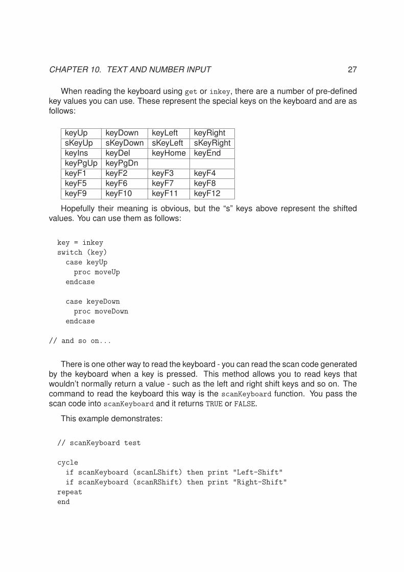
When reading the keyboard using get or inkey, there are a number of pre-definedkey values you can use. These represent the special keys on the keyboard and are asfollows:
keyUp keyDown keyLeft keyRight
sKeyUp sKeyDown sKeyLeft sKeyRight
keyIns keyDel keyHome keyEnd
keyPgUp keyPgDn
keyF1 keyF2 keyF3 keyF4
keyF5 keyF6 keyF7 keyF8
keyF9 keyF10 keyF11 keyF12
Hopefully their meaning is obvious, but the “s” keys above represent the shiftedvalues. You can use them as follows:
key = inkey
switch (key)
case keyUp
proc moveUp
endcase
case keyeDown
proc moveDown
endcase
// and so on...
There is one other way to read the keyboard - you can read the scan code generatedby the keyboard when a key is pressed. This method allows you to read keys thatwouldn’t normally return a value - such as the left and right shift keys and so on. Thecommand to read the keyboard this way is the scanKeyboard function. You pass thescan code into scanKeyboard and it returns TRUE or FALSE.
This example demonstrates:
// scanKeyboard test
cycle
if scanKeyboard (scanLShift) then print "Left-Shift"
if scanKeyboard (scanRShift) then print "Right-Shift"
repeat
end
CHAPTER 10. TEXT AND NUMBER INPUT 28
The constants scanLShift, scanLShift, etc. maybe be displayed on the screenusing the scanKeys command in immediate mode. (You may need a long screen asthere are currently 233 scan codes).
Note that using scanKeyboard in your program and pushing printable keys will leavethose keys in the system input buffer ready for the next time your program performsa keyboard read using input, get, get$ or when the program exits and returns toimmediate mode. To throw away all these characters, you can use the clearKeyboard
instruction.

Chapter 11
Text and Number Output
RTB has a flexible output system that allows you to change the colour of the foregroundand background, change the font size, (simple scaling of height or width) and changethe screen location for the next character to be printed. You can also define your ownfont characters if required, and read existing font definitions.
The important thing to remember is that the text (and graphics) may not alwaysappear immediately on the screen. This is because all text and graphics output iswritten to a “shadow” display screen and this “shadow” screen is only sent to the actualdisplay screen under certain conditions:
• Using the cls, gr, or hgr instruction will clear and update the screen immediately.
• If your program stops for input using input, get or get$ instructions then thescreen will be updated.
• You print something and the updateMode system variable is set to 1 or 2.
11.1 updateMode
The updateMode system variable controls how and when the screen is updated whenyou use a print instruction. You can change updateMode at any time during programexecution. The default value is 1 and this is set every time a program is run.
• updateMode = 0: The screen is never explicitly updated. This is the fastest way tooutput lots of text to the screen. It’s also the quickest way to frustration, howeverupdates will happen when your program stops for input, or you explicitly use theupdate instruction.
29

CHAPTER 11. TEXT AND NUMBER OUTPUT 30
• updateMode = 1: The screen is updated whenever your program prints some-thing that causes a new-line to be output. ie. a print instruction without a trailingsemicolon. Updates also happen when the program stops for input, as usual.This is the default mode.
• updateMode = 2: The screen is updated whenever your program prints anything.This is the slowest output mode, but can be useful in some circumstances.
For most text-based programs, having updateMode set to its default value of 1 issufficient and you should not have to do anything. The time you may need to manuallyforce an update would be when drawing graphics and you don’t want to stop yourprogram to read input (e.g. is using inkey or scanKeyboard).
print The print instruction is the command to print numbers and strings to the screen.It accepts any mix of numbers and strings, separated by the semicolon character.Normally a new-line is taken at the end, but if you add a trailing semicolon, thenthe newline is suppressed. This lets you use multiple print instructions to buildup a line.
numFormat (total, decimals) This affects all future number printing via the print
statement. The numbers will be printed right-justified in a total fields width oftotal with decimals digits after the decimal point. Setting the parameters bothto zero restores the default format which is designed to be general purpose.
cls The screen is cleared.
cls2 The screen is cleared, but not updated. See above for more details.
hvTab (x, y) The cursor is moved to the supplied column x and line y. Note that (0,0)is top-left of the text screen. See also the hTab and vTab system variables.
fontScale (x, y) This allows you to set the scaling factor for all subsequent text print-ing. If RTB was started with the -l flag, then a fontScale of (2,2) is assumed.When you execute this command, the cursor position (hvTab) is reset to (0,0),the top-left corner. You must then move the cursor using the hvTab or hTab= andvTab= instructions. The screen width and height will change to reflect the newfont size.
defChar (c, x0,x1,x2,x3,x4,x5,x6,x7,x8,x9) This lets you define (or re-define) char-acters in the internal font. Characters are 8 pixels wide by 10 pixels deep. c is thecharacter to re-define (0-255) and x0 through x9 are the 10 rows of 8 bits each.x0 is the top row and the most significant bit is the leftmost pixel. E.g.
defChar (129, 0x80, 0x40, 0x20, 0x10, 0x08, 0x04, 0x02, 0x01, 0xFF, 0xFF)
print chr$ (129)
end

CHAPTER 11. TEXT AND NUMBER OUTPUT 31
Note that you can’t redefine characters number 8, 10 or 13 as these correspondto backspace line-feed and carriage return.
11.2 Variables affecting output
In addition to updateMode above, the following apply to text output:
hTab Set or read the horizontal screen position. The left-most column is position zero.
vTab Set or read the vertical screen position. The top-line is line zero.
ink Set or read the foreground colour of the output text. See the colours section andthe colours.rtb demo program for more details.
paper Set or read the background colour of the output text. See the colours sectionand the colours.rtb demo program for more details.
tWidth This is the number of characters the current screen is wide. This changes ifyou use the fontScale instruction.
tHeight This is the number of characters the current screen is tall. This changes ifyou use the fontScale instruction.

Chapter 12
Conditionals: IF . . . THEN . . .
RTB has a comprehensive IF statement, but unlike traditional BASICs, you must usethe corresponding THEN statement with it.
// IF Statement example
INPUT "dummy value: ", dummy
IF dummy < 100 THEN PRINT "it’s < 100"
IF dummy = 42 THEN dummy = dummy + 1
PRINT "Dummy is "; dummy
END
The expression inside the IF ... THEN statement is evaluated as if it’s an assign-ment expression. If the result if 0, then its treated as FALSE, anything else is treatedas TRUE. See the section on operator precedence in the variables chapter for moredetails.
12.1 Multiple lines
We can extend the IF statement over multiple lines, if required. The way you do thisis by making sure there is nothing after the THEN statement and ending it all with theENDIF statement as this short example demonstrates:
// Program fragment to demonstrate multi-line IF
test = 42
IF test <> 15 THEN
PRINT "Test was not 15"
32

CHAPTER 12. CONDITIONALS: IF . . . THEN . . . 33
PRINT "We will end now"
END
ENDIF
PRINT "Test was 15"
PRINT "We can go home now"
END
12.2 IF . . . THEN . . . ELSE . . . ENDIF
We can modify the IF...THEN construct with one more keyword; ELSE This can providean alternative set of instructions to follow without using a GOTO instruction and can helpto make your programs more readable.
The following example demonstrates:
REM Guess
secret = 42
CYCLE
INPUT "Guess the number? ", guess
IF guess = secret THEN
PRINT "You Guessed it!"
END
ENDIF
IF guess < secret THEN
PRINT "Too low"
ELSE
PRINT "Too high"
ENDIF
REPEAT
There are a few simple rules to observe when using multi-line IF...THEN...ELSE state-ments.
• IF, THEN and ELSE must be on separate lines, with nothing after the THEN state-ment (Some programming languages allow you to put them on the same lines,RTB doesn’t)
• The IF, ELSE and ENDIF statements must be at the start of a line. ie. you can nothave them after a THEN statement.
CHAPTER 12. CONDITIONALS: IF . . . THEN . . . 34
• If you are executing a GOTO instruction after a THEN instruction then you need touse both THEN and GOTO. Some variants of BASIC allow just one or the other, butnot RTB. These do not work in RTB:
100 IF a = 5 THEN 120
120 IF b = 7 GOTO 155

Chapter 13
Conditionals: SWITCH and CASE. . .
There is another form of conditionals commonly known as the switch statement al-though it’s actual representation varys from one programming language to another.
Essentially, the SWITCH instruction allows you to test a value against many differentvalues, and execute different code depending on which one matches. It can oftensimplify the writing of multiple IF. . . THEN. . . ELSE statements.
It’s probably easier to explain by example:
INPUT a
SWITCH (a)
CASE 1, 2
PRINT "You entered 1 or 2"
ENDCASE
CASE 7
PRINT "You entered 7"
ENDCASE
DEFAULT
PRINT "You entered something else"
ENDCASE
ENDSWITCH
END
In this simple test, we input a number, then test it against a set of values. You can putany expression or variable inside the brackets on the SWITCH statement. What followsis lines of CASE statements and each CASE has one or more constant numbers after it.These numbers are matched against the value of the SWITCH instruction and if there is a
35

CHAPTER 13. CONDITIONALS: SWITCH AND CASE. . . 36
match then the code after the CASE is executed up to the ENDCASE instruction and at thatpoint, control is transferred to the statement after the matching ENDSWITCH statement.Optionally you can use the instruction DEFAULT and this section will be executed if thereare no other matches.
Like IF. . . THEN. . . ELSE, SWITCH has a few simple rules:
• Every SWITCH must have a matching ENDSWITCH statement.
• Every CASE or DEFAULT statement must have a matching ENDCASE statement.
• Statements after a CASE statement must not run-into another CASE statement.(Some programming languages do allow this, but not RTB)
• The constants after the CASE statement (and the expression in the SWITCH state-ment) can be either numbers or strings, but you can’t mix both.
Finally, if you are reading some older BASIC programs, you may see a constructlike ON. . . GOTO. . . Our SWITCH statement is the modern way to handle code like this andif you are converting older programs it should be relatively simple to use the newerSWITCH instructions to help eliminate the issues keeping track of line numbers. Anexample:
Old Way:
100 ON a GOTO 200,300,400
120 PRINT "a was NOT 1, 2 or 3"
130 STOP
200 PRINT "a was 1"
210 GOTO 500
300 PRINT "a was 2"
310 GOTO 500
400 PRINT "a was 3"
410 GOTO 500
500 PRINT "Do something else now"

CHAPTER 13. CONDITIONALS: SWITCH AND CASE. . . 37
New way:
SWITCH (a)
CASE 1
PRINT "a was 1"
ENDCASE
CASE 2
PRINT "a was 2"
ENDCASE
CASE 3
PRINT "a was 3"
ENDCASE
DEFAULT
PRINT "a was NOT 1, 2 or 3"
STOP
ENDCASE
ENDSWITCH
PRINT "Do something else now"
So the new way is a bit longer and more to type, but it has the advantage of not relyingon line numbers and if we use the indentation as a guide, we can quickly scan down tofind the matching ENDSWITCH statement.

Chapter 14
Looping the Loop
This chapter explains the RTB instructions for handling loops. Using these instructions,you can almost always eliminate the use of the GOTO instruction, and hopefully makeyour program easier to read.
There are two new commands which RTB has to define a block of code which willbe repeated. These are: CYCLE which defines the start of the block and REPEAT whichdefines the end.
14.1 CYCLE . . . REPEAT
On their own, these would cause a program to loop between them forever, howeverRTB provides 3 means to control these loops. Lets start with an example.
// Demonstration of CYCLE...REPEAT
count = 1
CYCLE
PRINT "5 * "; count; " = "; 5 * count
count = count + 1
REPEAT
END
If you enter and RUN this program, it will run forever until you hit the ESC key, so it’s notthat useful for anything other than to demonstrate CYCLE and REPEAT.
You can use an IF ... THEN GOTO sequence to jump out of the loop, but that’s notvery elegant and we’re trying to not use GOTO anyway. Fortunately there are severalmodifiers.
38

CHAPTER 14. LOOPING THE LOOP 39
14.1.1 UNTIL
Changing it to:
// Demonstration of CYCLE...REPEAT
count = 1
CYCLE
PRINT "5 * "; count; " = "; 5 * count
count = count + 1
REPEAT UNTIL count > 10
END
and run the program again. We get our 5 times table, as before, but not a GOTO insight. We can see clearly the lines of code executed inside the loop and if we read theprogram it possibly makes more sense. We also don’t need to keep track of any linenumbers either.
14.1.2 WHILE
If we test the condition at the end of the loop (using UNTIL) then the loop will be ex-ecuted at least once. There may be some situations where we don’t want the loopexecuted at all, so to accomplish this we can move the test to the start of the loop,before the CYCLE instruction, but rather than use the UNTIL instruction we now useWHILE.
Note that you can use WHILE or UNTIL interchangeably. So you can re-write the aboveas:
// Demonstration of CYCLE...REPEAT
count = 1
WHILE COUNT <= 10 CYCLE
PRINT "5 * "; count; " = "; 5 * count
count = count + 1
REPEAT
END
or
// Demonstration of CYCLE, REPEAT...WHILE/UNTIL
count = 1
UNTIL COUNT > 10 CYCLE

CHAPTER 14. LOOPING THE LOOP 40
PRINT "5 * "; count; " = "; 5 * count
count = count + 1
REPEAT
END
Finally (in this section!) note that not all programing languages are as flexible as!this – some only allow WHILE at the top of a loop and UNTIL (or their equivalents) at thebottom.
14.2 For Loops
There is another form of loop which combines a counter and a test in one instruction.This is a standard part of most programming languages in one form or another and isoften called a “for loop”.
Here is our five times table program written with a for loop:
// Demonstration of FOR loop
FOR count = 1 TO 10 CYCLE
PRINT "5 * "; count; " = "; 5 * count
REPEAT
END
The FOR loop works as follows: It initialises the variable (count in this instance) to thevalue given; 1, then executes the CYCLE...REPEAT loop, adding one to the value of thevariable until the variable is greater than the end value 10.
There is an optional modification to the FOR loop in that allows you to specify howmuch the loop variable is incremented (or decremented!) by at each iteration by usingthe STEP instruction.
// Demonstration of FOR loop with STEP
FOR count = 1 TO 10 STEP 0.5 CYCLE
PRINT "5 * "; count; " = "; 5 * count
REPEAT
END
This will print our 5 times table in steps of 0.5.
Note that that the end number (10 in this case) isn’t tested for exactly. The test isactually >= So if you were incrementing by 4 (for example), count would start at 1,
CHAPTER 14. LOOPING THE LOOP 41
then become 5, then 9, then 13 – at which point flow control would jump to the lineafter the REPEAT.
Another way to visualise the FOR loop is like this:
// Demonstration of how a FOR loop works
// ... FOR count = 1 to 10 STEP 0.5 CYCLE ...
count = 1
WHILE count <= 10 CYCLE
PRINT "5 * "; count; " = "; 5 * count
count = count + 0.5
REPEAT
END
the FOR loop is simply a convenient way to incorporate the three lines controlling count
into one line.
14.3 Breaking and continuing the loop
There are two other instructions you can use with CYCLE...REPEAT loops – BREAK whichwill cause program execution to continue on the line after the REPEAT instruction, ie.You break out of the loop, and CONTINUE which will cause the loop to re-start at the linecontaining the CYCLE instruction, continuing a FOR instruction and re-evaluating and anyWHILE or UNTIL instructions.
Chapter 15
Data, Read and Restore
Sometimes you need to initialise variables with a predetermined set of data – numbersor strings. BASIC and RTB has a relatively easy, if somewhat old-fashioned1 way to dothis.
There are three keywords to control this. This first is the DATA instruction. Thisdoesn’t do anything in its own right, but serves as a marker or placeholder for thedata. After the DATA instruction, you list data values, numbers or strings separated bycommas, as this example demonstrates:
DATA 1, 2, 17.4
DATA "Monday", "Tuesday", "Wednesday, "Thursday"
DATA "Friday,", "Saturday", "Sunday", 7
Note that you can mix numbers and strings on the same line.
To get data into your program variables, we use the READ instruction. We can readone, or many items of data at a time.
READ start, end, number
READ day1$, day2$
and so on.
RTB remembers the location of the last item of data read, so that the next readcontinues from where it left off. If you try to read more data than there is defined thenyou’ll get an error message and the program will stop running.
1Old-fashioned in that hardly any other modern languages use this method, but it’s still useful in thisenvironment
42

CHAPTER 15. DATA, READ AND RESTORE 43
You can reset RTBs data pointer with the RESTORE command. On its own, it willreset it to the very first DATA statement, but you can give it a line number to set the datapointer to the first data item on that line.
100 RESTORE 1000
110 READ day$
120 PRINT day$
130 RESTORE 1000
140 READ day$
150 PRINT day$
160 END
1000 DATA "Monday", "Tuesday", "Wednesday, "Thursday"
1010 DATA "Friday,", "Saturday", "Sunday", 7
With the above set of data statements, this will print Monday twice.
You need to use line-numbers to use RESTORE with a line number! This should notbe needed for most uses though.
Data statements can be anywhere in your program – they are ignored by the inter-!preter and only used for READ instructions, however this does mean that we need totrack line numbers to remember where our data is if using the RESTORE instruction. . .I recommend that you place your data at the very end of your program with high linenumbers (or no line numbers at all!) to make it easier to work out where the data is andto keep track of it.
Here is an example which calculates the average of a set of numbers:
// Calculate the average of a set of numbers and print
// out numbers below, equal to or above average
READ numNumbers
DIM table (numNumbers)
FOR i = 0 to numNumbers - 1 CYCLE
READ table (i)
REPEAT
// Average
total = 0
FOR i = 0 to numNumbers - 1 CYCLE
total = total + table (i)
REPEAT
average = total / numNumbers

CHAPTER 15. DATA, READ AND RESTORE 44
PRINT "The average is "; average
// Print all numbers
FOR i = 0 to numNumbers - 1 CYCLE
PRINT "Number "; i + 1; " = "; table (i); " ";
IF table (i) < average THEN PRINT "below"
IF table (i) > average THEN PRINT "above"
IF table (i) = average THEN PRINT "average"
REPEAT
END
DATA 10
DATA 1,2,3,4,5,6,7,8,9,0

Chapter 16
Miscellaneous Program instructions
Procedures listed here are not part of any one subsystem, (e.g. graphics) so are listedhere for convenience.
wait (time) This waits for time seconds. This may be a fractional number, but theaccuracy will depend on the computer you are running it on, however delaysdown to 1
100th of a second or better should be achievable.
STOP Program execution is stopped with an message indicating the current line num-ber. You may use the CONT command to continue your program at the line afterthe STOP instruction.
END Program execution is ended normally.
SWAP (v1, v2) This swaps the value of the 2 variables round. Both arguments mustbe the same type - ie. both numeric or both string, and both must be scalar (ie.ordinary variables, not array elements)
45

Chapter 17
Numerical Functions and data
Functions and system variables, etc. that return and deal with numbers.
17.1 System variables and constants
PI, PI2 System constants that return the approximate value of π and π
2respectively.
E.g.
area = PI * radius * radius
SEED This can be assigned to to initialise the random number generator, or you canread it to find the current seed.
TIME This returns a number which represents the time that your program has beenrunning in milliseconds. It is initialised to zero when your program starts. E.g.
print "Wait for it..."
wait (2)
print "Press the spacebar... "
start = TIME
cycle
// Do nothing
repeat until get$ = " "
now = TIME
print "You took: "; (now - start) / 1000; " seconds."
end
DEG Switches the internal angle system to degrees. There are 360 degrees in a fullcircle. This is the default mode when a program starts.
46

CHAPTER 17. NUMERICAL FUNCTIONS AND DATA 47
RAD Switches the internal angle system to radians. There are 2π radians in a full circle.
CLOCK Switches the internal angle system to clock mode. There are 60 minutes in afull circle.
17.2 Functions
RND (range) This function returns a random number based on the value of range. Ifrange is zero, then the last random number generated is returned, if range is 1,then a random number from 0 to 1 is returned, otherwise a random number from0 up to, but not including range is returned.
SIN (angle) Returns the sine of the given angle.
ASIN (x) Returns the arc sine of the supplied argument x
COS (angle) Returns the cosine of the given angle.
ACOS (x) Returns the arc cosine of the supplied argument x
TAN (angle) Returns the tangent of the given angle.
ATAN (x) Returns the arc tangent of the supplied argument x
ABS (x) Returns the absolute value of the supplied argument x ie. if the argument isnegative, make it positive.
EXP (x) Returns the value of ex
LOG (x) Returns the natural logarithm of x
SQRT (x) Returns the square root of x
SGN (x) Returns -1 if the number is negative, 1 otherwise. (Zero is considered posi-tive)
INT (x) Returns the integer part of x
HASH (string, modulo) Returns a hash value based on the string and modulo. Thevalue returned is between 0 and modulo. This function is used internally in RTBfor the associative array indexing. The hash function is based on the function inThe Practice of Programming (HASH TABLES, pg. 57)
MAX (x, y) Returns the larger of x or y
MIN (x, y) Returns the smaller of x or y

CHAPTER 17. NUMERICAL FUNCTIONS AND DATA 48
VAL (string$) Returns the number represented by string$. e.g. ”1234” would returnthe number 1234. This is the opposite of the STR function.
ASC (string$) Returns the ASCII value represented by the first character of string$.e.g. ”A” would return 65. It is the opposite of the CHR$ function.
LEN (string$) Returns the number of characters in string$.

Chapter 18
String Functions and data
Functions and system variables, etc. that return and deal with strings.
18.1 System variables
DATE$ This returns a string with the current date in ISO 8601 format: YYYY-MM-DD.
TIME$ This returns a string with the current time of day in ISO 8601 format: HH:MM:SS.
Date and Time example program:
now$ = TIME$
today$ = DATE$
print "full date & time: "; today$; " "; now$
end
18.2 Functions
CHR$ (num) This function returns a string from the ASCII value of num It is the oppositeof the ASC function. e.g. CHR$ (65) returns ”A”.
LEFT$ (string$, len) Returns the leftmost len characters of string$.
E.g. LEFT$ ("Hello", 2) would return "He".
RIGHT$ (string$, len) Returns the rightmost len characters of string$.
E.g. RIGHT$ ("Hello", 2) would return "lo".
49

CHAPTER 18. STRING FUNCTIONS AND DATA 50
MID$ (string$, start, len) Returns the middle len characters of string$ startingfrom position start. the first character of the string is at index position zero.
e.g. MID$ ("Hello", 1,2) would return "el".
SPACE$ (len) Returns a string of length len comprising of spaces.
STR$ (num) Returns a string version of the supplied number num. e.g. STR$ (42.42)
would return "42.24". This is the opposite of the VAL function.

Chapter 19
Graphics
RTB supports two types of graphics; traditional 2-D Cartesian (x, y) type graphics withfunctions to plot points, lines, etc. and turtle graphics which can sometimes be easierto teach/demonstrate to younger people.
RTB normally works in the highest graphical resolution available to it, but it also sup-ports two effective resolutions - the high resolution is the native resolution of the displayyou are using - e.g. on a PC monitor this may be up to 1280x1024, or 1920x1080 onan HD monitor. It also supports a lower resolution where each low resolution pixel isreally 8x8 high resolution pixels.
Your programs should use the gWidth and gHeight system variables to scale theiroutput to the current display size. Assuming a fixed resolution may not be advisable forprograms designed to run on systems other than your own.
Note: In all the graphical instructions that take an x, y coordinate, this refers to thebottom left hand point if it’s a rectangle. Similarly where you see w, h this refers to awidth and height, extending to the right and above the corresponding x, y coordinate.
19.1 System Variables
colour This can be assigned to, or read from, and represents the current plottingcolour. E.g.
colour = Yellow
gWidth This can be read to find current width of the display in either high resolution orlow resolution pixels.
51

CHAPTER 19. GRAPHICS 52
gHeight This can be read to find the current height of the display in either high resolu-tion or low resolution pixels.
tAngle This can be read or assigned to and represents the current angle of the turtlewhen using turtle graphics mode. The angle returned will be expressed in theangular units used when the last left() or right() instruction was executed.
See also the colour names and note the current angle modes (degrees, radians orclock) when using turtle graphics or any trig. functions to plot graphics.
19.2 General Graphics
hgr This clears the screen and initialises high-resolution graphics mode. This is thedefault at startup time.
gr This clears the screen and initialises low-resolution graphics mode.
saveScreen (filename$) This takes a snapshot of the current screen and saves it tothe filename given.
saveRegion (filename$, x, y, w, h) This takes a snapshot of the region identifiedby x, y (bottom left corner) and the width and height identified by w, h
loadImage (filename$) This loads the given image into memory and returns an iden-tifier to the image which can be used in subsequent plotImage commands. Mostimage formats are accepted - JPG, PNG, BMP, GIF, TIFF, etc.
plotImage (id, x, y) This plot the image identified by id from a previous loadImage
command at the given x,y location (bottom left). You can plot the same imagemany times at any location on the screen. The image is clipped is all or part of itwould be off-screen.
getImageW (id), getImageH (id) These functions return the width and height re-spectively of a loaded image.
Example:
// Tile an image
id = loadImage ("selfie.jpg")
w = getImageW (id)
h = getImageH (id)
for x = 0 to gWidth step w cycle
for y = 0 to gHeight step h cycle
plotImage (id, x, y)

CHAPTER 19. GRAPHICS 53
repeat
repeat
end
copyRegion (x1, y1, w, h, x2, y2) This copies an area of the screen from oneplace to another. The starting region is identified by the x1, y1 location (bottomleft), and width and height identified by w, h. This is copied to the new locationidentified by x2, y2
scrollUp (x, y, w, h, lines) This scrolls the region identified by x, y, w, h up ordown by lines lines.
scrollDown (x, y, w, h, lines)
scrollLeft (x, y, w, h, lines)
scrollRight (x, y, w, h, lines) As above, but scrolls the region down, left or right.
rgbColour (r, g, b) This sets the current graphical plot colour to an RGB (Red,Green, Blue) value. The values should be from 0 to 255.
update When plotting graphics, (and text) they are actually plotted to a separate off-screen working area, so if you write a program that does lots and lots of graphicalactions, then you may not see the display being updated. The update procedureforces the working area to be copied to the display. An update is also performedautomatically if your program stops for input. (input, get, get$), and also atoutput (via the print instruction) depending on the setting of updateMode.
getPixel (x, y) This returns the standard colour of the pixel at the supplied x,y loca-tion on the screen. If the colour of the pixel is not one of the 16 standard colours,then -1 is returned.
getPixelRBG (x, y) This returns the 24-bit value of the pixel at the supplied x,y lo-cation on the screen. See the following example program for its use:
rgbColour (1,2,3)
plot (0,0)
pixel = getPixelRGB (0,0)
print "Pixel is: "; pixel
r = (pixel >> 16) & 0xFF
g = (pixel >> 8) & 0xFF
b = (pixel >> 0) & 0xFF
print "r: "; r; ", g: "; g ; ", b: "; b
end
CHAPTER 19. GRAPHICS 54
19.3 Cartesian Graphics
The graphical origin at (0,0) is at the bottom-left of the display. Coordinates may benegative and may also be off-screen when lines are clipped to the edge of the display.The ORIGIN command may be used to change the graphical origin.
plot (x, y) This plots a single pixel in the selected graphics mode in the selectedcolour. Note that (0,0) is normally bottom left.
hLine (x1, x2, y) Draws a horizontal line on row y, from column x1 to column x2.
vLine (y1, y2, x) Draws a vertical line on column x, from row y1 to row y2.
line (x1, y1, x2, y2) Draws a line from point x1, y1 to x2, y2.
lineTo (x1, y1) Draws a line from the last point plotted (by the plot or line proce-dures to point x1, y1.
circle (cx, cy, r, f) Draws a circle at (cx,cy) with radius r. The final parameter,f is either TRUE or FALSE, and specifies filled (TRUE) or outline (FALSE).
ellipse (cx, cy, xr, yr, r, f) Draws an ellipse at (cx,cy) with x radius xr andy radius yr. The final parameter, f is either TRUE or FALSE, and specifies filled(TRUE) or outline (FALSE).
triangle (x1, y1, x2, y2, x3, y3, f) Draws a triangle with its corners at the threegiven points. The final parameter, f is either TRUE or FALSE, and specifies filled(TRUE) or outline (FALSE).
polyStart This marks the start of drawing a filled polygon.
polyPlot (x, y) This remembers the given X,Y coordinates as part of a filled poly-gon. Nothing is actually drawn on the screen until the polyEnd instruction isexecuted. Polygons can have a maximum of 64 points.
polyEnd This marks the end of drawing a polygon. When this is called, the storedpoints will be plotted on the screen and the polygon will be filled.
rect (x, y, w, h, f) Draws a rectangle at (x,y) with width w and height h. Thefinal parameter, f is either TRUE or FALSE, and specifies filled (TRUE) or outline(FALSE).
origin (x, y) This changes the graphics origin for the Cartesian plotting procedures.The x, y coordinates are always absolute coordinates with (0,0) being bottomleft.

CHAPTER 19. GRAPHICS 55
19.4 Turtle Graphics
When the graphics are initialised with either GR or HGR, the turtle position is set tothe middle of the screen, pointing at an angle of 0 degrees (up) with the pen lifted.However note that the turtles position is affected by the origin command above, soyou may have to take this into consideration if using origin.
With the noted effects of the origin procedure, you may mix turtle and Cartesiangraphics without any issues.
penDown This lowers the “pen” that the turtle is using to draw with. Nothing will bedrawn until you execute this procedure.
penUp This lifts the “pen” that the turtle uses to draw. You can move the turtle withoutdrawing while the pan is up.
move (distance) This causes the turtle to move forwards distance screen pixels.
moveTo (x, y) This moves the turtle to the absolute location (x, y). A line will bedrawn if the pen is down.
left (angle) Turns the turtle to the left (counter clockwise) by the given angle.
right (angle) Turns the turtle to the right (clockwise) by the given angle.
19.5 Sprites
Sprites are (usually) small bitmap images which you can plot to the screen under pro-gram control. You can create them using one of the many graphical image creationpackages available. RTB accepts many different file formats for sprites but you arestrongly recommended to use a “non-lossy” format such as BMP, GIF, PNG, etc. toavoid any block/aliasing effects in e.g. JPG.
RTB can handle up to 1024 sprites and each sprite can have up to 64 sub-sprites.(If you’re used to programming in Scratch, think of the sub-sprites as “costumes”) Allsub-sprites in one sprite should have the same dimension.
Sprites “float” above the background image, and above each other. The first spriteplotted to the screen is above the background image, then 2nd sprite plotted is abovethat and so on. The sub-sprites can be used to perform simple animations - e.g. aspace invader might have 2 sub-sprites in each sprite to give the illusion of its legsmoving as it moved over the screen. A “pacman” sprite could have 3 or 4 sub-spritesto represent the various stages of the “mouth” moving from open to closed.
CHAPTER 19. GRAPHICS 56
The position of a sprite on the screen is affected by three parameters. The first isthe supplied x, y coordinates and this is adjusted by the sprites own origin position(see setSpriteOrigin below), and finally by the global graphics origin setting.
To move a sprite over the screen, all you need to do is update its position with theplotSprite instruction. The system takes care of un-plotting it and plotting it in thenew position.
Typically you would draw the background, then:
cycle
// plot the sprites
update
repeat
newSprite (subSprites) This initialises some storage and structures to take a newsprite and a stack of “sub sprites”. Once you have created the sprite in this wayyou need to load the individual image(s) into it. The return value is a handle thatyou must use when referencing this sprite in future operations. E.g.
// create a new sprite with space for just one sub-sprite
spr1 = newSprite (1)
loadSprite (filename$, sprite, subSprite) This loads a sprite from the suppliedfile into memory. sprite is the handle returned by the newSprite instruction andsubSprite is the sub-sprite index. E.g.
loadSprite ("test.png", spr1, 0) // subSprite starts at zero
setSpriteTrans (sprite, r, g, b) This sets the transparency mask on the givensprite. It is applies to all sprites in the stack, so they should all use the samecolour to represent the transparent colour.
Note: On the Raspberry Pi, the graphics are 16 bits per pixel, so the actual RGB!values may be different to what you’re expecting. A typical value might be red:247, green: 251, blue: 247.
plotSprite (sprite, x, y) This plots the given sprite sprite at the suppled x, y
coordinates. The coordinates normally specify the bottom-left corner of the bound-ing rectangle of the sprite but may be moved with the setSpriteOrigin instruc-tion.
setSpriteOrigin (sprite, x, y) This sets the origin point inside a sprite (and allsub sprites). Note that if you want to set the origin to the exact middle of thesprite then the sprite has to be an odd number of pixels wide and high.
CHAPTER 19. GRAPHICS 57
hideSprite This removes a sprite from the screen on the next update.
getSpriteW (sprite) This returns the width of the sprite indicated by sprite.
getSpriteH (sprite) This returns the height of the sprite indicated by sprite.
spriteCollide (sprite) This is a fast “bounding box” sprite collision test. It takes thesprite identified by sprite and searches the other sprites to see if it has collided.It returns the sprite identifier of the first sprite it has collided with, or -1 if it’s notin collision.
spriteCollidePP (sprite, accuracy) This is a slow “perfect pixel” sprite collisiontest. It takes the sprite identified by sprite and searches the other sprites to seeif it has collided within the accuracy specified. It returns the sprite identifier of thefirst sprite it has collided with, or -1 if it’s not in collision.
The accuracy is expressed in pixels and should be from 1 (best) to 16 (poor, butstill usable). It all depends on the amount of overlap your application can tolerate.
You do not have to erase a sprite from the screen when you move it, just callplotSprite with the new coordinates.

Chapter 20
Mouse Input
RTB can use the mouse connected to your system. You can enable or disable it, readits position and button states. You can even move it to a new location on the screen.
Moving the scroll wheel on the mouse has the same effect as pushing the up anddown arrow keys on the keyboard.
mouseOn This turns on the visible mouse cursor on the screen. It’s probably a goodthing to call this before reading its position.
mouseOff This removed the mouse cursor from the screen.
getMouse (x, y, z) This returns the x, y location of the mouse as well as a variablez this represents the buttons on the mouse. Bits 0, 1 and 2 of z represent theLeft, right and middle mouse button respectively. Any origin set with the origin
instruction is taken into account, so if you set origin (gWidth / 2, gHeight /
2) then with the mouse in the middle of the screen, the returned coordinate willbe 0,0.
setMouse (x, y) This sets the mouse position to the supplied x,y coordinate. Thecurrent origin is taken into account as with getMouse above.
58
Chapter 21
Sound
RTB has several different ways to make sound. You can play background music, soundsamples, simple tones and synthesised sounds based on the old BBC Micro SOUNDand ENVELOPE commands.
Internally, all sound samples, music, etc. is held as 8-bit, mono at 11025 samplesper second. This is more for efficiency on the Raspberry Pi than anything else.
21.1 Music
Music is intended to be used as a background to your program. Most file formats arerecognised. E.g. WAV, MP3, etc. RTB can load as many different music files as it hasmemory for and you can start/stop, pause and resume the music track.
loadMusic (filename$) This loads a music file into memory for later playing and re-turns an identifier than can be used in subsequent calls to playMusic, etc.
playMusic (id, repetitions$) This starts playing the previously loaded music iden-tified by id for repetitions times. If any music is currently playing, it is stoppedand the new music is started.
stopMusic Stops any music that may be playing.
pauseMusic Temporarily stops any music that may be playing.
resumeMusic Resumes playing any previously paused music.
setMusicVol (volume) Sets the volume of the music channel to volume. The volumeis expressed as a percentage; 0 to 100.
59
CHAPTER 21. SOUND 60
21.2 Sound Samples
As with music, sound samples can be in several different formats. WAV, MP3, andothers are supported. RTB can load as many samples as it has memory for but canonly play 4 at once.
loadSample (filename$) This loads a sample file into memory for later playing andreturns an identifier than can be used in subsequent calls to playSample, etc.
playSample (handle, channel, loops) This plays the previously loaded sample iden-tified by handle on the supplied channel for the given number of loops. Slightlydifferent from playMusic above in that this is the number of loops and not thenumber of repetitions, so it needs to be 1 to play once.
There are 4 channels available, numbered 0 through 3.
stopChan (channel) Stops the sound sample playing on the given channel.
pauseChan (channel) Pauses the sound sample playing on the given channel.
resumeChan (channel) Resumes the sound playing on a previously paused soundchannel.
setChanVol (channel, volume) Sets the channel volume on the given channel. Thevolume is expressed as a percentage; 0 to 100.
21.3 Tones and Sounds
There are four channels for tone/sound playing; 0, 1, 2 and 3. Channel 0 alwaysgenerates white noise. The sound system will queue one sound per channel (ie. itwill return immediately the sound starts playing) so its possible to execute three tone
instructions one after the other on different channels to play a simple chord, or you usethe sound instruction to do this automatically.
tone (channel, volume, frequency, duration) This plays a simple tone on the givenchannel of the given frequency. The volume is expressed as a percentage; 0 to100. The duration is in seconds and may be fractional. The longest tone you canplay is 20 seconds in duration. E.g. Play concert A (440Hz) for 1 second:
tone (1, 30, 440, 1)
Playing a C major chord:

CHAPTER 21. SOUND 61
tone (1,30, 261, 1)
tone (2,30, 330, 1)
tone (3,30, 392, 1)
sound (channel, volume, pitch, duration) The sound instruction seems similar tothe tone instruction, but its much more complex and can be used in conjunctionwith the envelope instruction to generate comple sounds and tones.
• channel: 0, 1, 2 or 3. Channel 0 generates white noise.
• volume: 0 to -15 to select one of 16 volume levels (0 is silent, -15 is fullvolume), or a positive number to identify the envelope to use.
• pitch: The pitch value - this is not the same as the frequency in the tonecommand. See the table at the end for a list of pitch vs. piano note values.
• duration: This is the duration of the note in 20ths of a second intervals.
envelope (...) the envelope instruction is somewhat complex and takes 14 parame-ters. they are:
• id: This is the identifier for this envelope. You can create up to 8 envelopesnumbered 1 through 8.
• stepLen: This is the number of 100ths of a second that each pitch or ampli-tude step takes.
• dP1, dP2, dP3: These represent the change (delta) in pitch for each of thethree corresponding step times (pStepsX), in intervals of stepLen 100th of asecond.
• pSteps1, pSteps2, pSteps3: These represent the number of steps of stepLen100ths of a second for pitch (dPX) change.
• aRate, dRate, sRate, rRate: The rate of change of the volume during theattac, decay, sustain and release phase of the note. The release phase isnot implemented here - the note ends at the end of the sustain phase.
• targetAttack, targetDecay: This is the target volume level (0-127) of thenote at the end of the attack or decay phase.
Note:More to come, but read any document on the BBC Micro sound and enve-!lope command for more details.

Chapter 22
File and System program handling
22.1 File handling
RTB supports reading and writing of ordinary text files. There are two main methods offile accessing; sequential and random-access. When you open a file, it is assigned anumerical “handle” and you need to use this handle when performing other operationson the file. RTB allows you to open multiple files at the same time, up to a limit set bythe implementation. (64 by default). Each open file will have a unique handle, whichyou must keep track of when manipulating files.
All data written to, or read from a file is textual in nature. You can not write binarydata in RTB. Numbers are stored as literal strings as if they ha: been printed on thescreen. (And in particular, the format set by the numFormat instruction is used whenprinting numbers into files).
22.2 Sequential access
Sequential file access is straightforward. You open a file, then read from it, or write toit. You can reset the file pointer to the start of the file using the rewind instruction, soyou can write data to a file, then rewind, then read the data back again. There is nostructure to the file other than what you write into it yourself. ie. if you want to read the15th line in a file, then you need to read the preceding 14 lines unless you know theexact line length of each line, then you can use the seek instruction to jump to that line,but if the lines are all different length, then you need to read the while file from start toend.
62
CHAPTER 22. FILE AND SYSTEM PROGRAM HANDLING 63
22.3 Random access
Random file access is similar to sequential, however it additionally allows you to splityour file into fixed-size records, then you can seek to any of these records at random.
There are no special instructions that make a file any different when in sequentialmode to random mode other than those you code yourself. You must plan the recordsize (in bytes or characters) beforehand and you must always seek to the correct recordin your file before reading or writing. Each record is then treated like a small sequentialfile and you can read and write into it - however you must make sure that you don’t writemore data into the record than you have planned for, otherwise that data will overflowinto the next record with unpredictable results.
Random access files can be wasteful of disk space, but they can also be a fastan versatile method of storing and retrieving data. Most modern databases use thistechnique to store data for fast retrieval.
The functions here only return a simple error code - usually -1 in cases of file notfound, or insufficient access rights to open the file.
22.4 File handling instructions
openIn (filename$) This function opens a file and makes it available for input only. Anumeric handle associated with the file is returned, or -1 is returned on any fileerror (e.g. file not found)
openOut (filename$) This function opens a file and makes it available for output only.A numeric handle associated with the file is returned or -1 if there was an er-ror when trying to open/create the file. The file is created if it doesn’t exist, ortruncated to zero length if it does exist.
openUp (filename$) This function opens a file and makes it available for reading orwriting (ie. updating) A numeric handle associated with the file is returned or -1if there was an error when trying to open the file. The file is created if it doesn’texist.
close (handle) The file identified by the supplied handle is closed and all data iswritten to disk. Subsequent read or writes to the file will return an error.
eof (handle) This function returns a TRUE or FALSE indication of the state of the filepointer when reading the file. It is an error to try to read past the end of the file,so if you are reading a file with unknown data in it, then you must check at welldefined intervals (e.g. before each input#.

CHAPTER 22. FILE AND SYSTEM PROGRAM HANDLING 64
rewind (handle), ffwd (handle) These instructions move the file pointer back to thestart of the file or to the end of the file respectively. If you want to append data tothe end of an existing file, then you need to use openUp followed by ffwd beforewriting the data.
seek (handle, offset) This instruction moves the file pointer to any place in the file.It can even move the file pointer beyond the end of the file in which case the fileis extended. The argument suppled to seek is an absolute number of bytes fromthe start of the file. If you are using random access files and want to access the7th record in the file, then you need to multiple your record size by 7 to work outthe location to seek to.
print# handle, ... This instruction acts just like the regular print instruction exceptthat it sends data to the file identified by the supplied file-handle rather than tothe screen. Numbers are formatted according to the settings of numFormat. Itis strongly recommended to only print one item per line if you are going to readthose items back into an RTB program again.
// Append data to the end of a file
myFile = openUp ("testfile.txt")
ffwd (myFile)
print# myFile, "Appended line"
close (myFile)
input# handle, variable This works similarly to the regular input instruction, butreads from the file identified by the supplied file-handle rather than from the key-board.
// Copy file to screen
myFile = openIn ("testfile.txt")
while not eof (myFile)
input# myFile, line$
print line$
close (myFile)
The popenOut, and pOpenIn functions use the existing print# and input# instruc-tions. See the file handling section for more details on these.
22.5 Calling system programs
RTB programs can call existing system programs via three different ways. These in-structions are mentioned in this chapter as they share some of the above file handlinginstructions.

CHAPTER 22. FILE AND SYSTEM PROGRAM HANDLING 65
system (filename$) This function calls a system program. RTB program execution issuspended while the program is running. Input to the program and output fromthe program is not avalable, and there is no notification of error from the program.
pOpenIn (filename$) This function opens a program and makes it available for inputonly. A numeric handle associated with the file is returned, or -1 is returned onany file error (e.g. file not found)
Use input# to read data from the program.
// Test the pOpenIn function
x = pOpenIn ("/bin/ls -l /var") // Open the ls program for input
while not eof (x) cycle
input# x, a$
print a$
repeat
pClose (x)
END
popenOut (filename$) This function opens a program and makes it available for out-put only. (ie. data from your RTB program output and fed into the system pro-gram) A numeric handle associated with the file is returned or -1 if there was anerror when trying to open/create the file. The file is created if it doesn’t exist, ortruncated to zero length if it does exist.
Use print# to send data to the program.
Chapter 23
Serial Port Programming
RTB supports a few instructions to allow you to send and receive data over serial ports.These go by various names, a common one being RS232.
Moderns PCs often lack a directly connected serial port, so you may have to usea USB connected device. Using them is the same whether directly connected or viaUSB. The important thing to know is the name of the serial device. For directly con-nected devices, this might be something like ”/dev/ttyS1”, or for USB devices it mightbe something like /dev/ttyUSB0. Occasionally you have find a /dev/ttyACM0 for someolder USB devices. The Raspberry Pi’s on-board serial port is called /dev/ttyAMA0.
sOpen (filename$, baud) This opens a serial device and makes it available for ouruse. It takes the name of the serial port and the speed as an argument andreturns a number (the handle) of the device. We can use this handle to referencethe device and allow us to open several devices at once. Example:
arduino = sOpen ("/dev/ttyUSB0", 115200)
Most standard baud rates are recognised. The device is always opened with thedata format set to 8 data bits, 1 stop bit and no parity. All handshaking is turnedoff.
sClose (handle) This closes a serial port and frees up and resources used by it. It’snot strictly necessary to do this when you end your program, but it is consideredgood practice.
sGet (handle), sGet$ (handle) Fetch a single byte of data from an open serial portand return the data as a number or a single character string. This function willpause program execution for up to 10 seconds if no data is available. If there isstill not data after 10 seconds, the function will return -1 or an empty string.
66

CHAPTER 23. SERIAL PORT PROGRAMMING 67
sPut (handle. data), sPut$ (handle, data) Send a single byte of data, or a stringof characters to an open serial port. Example:
SPUT (arduino, 64)
SPUT$ (arduino, "Hello")
sReady (handle) Returns the number of characters available to be read from an openserial port. This can be used to poll the device to avoid stalling your programwhen there is no data available to be read.
Chapter 24
Minecraft
RTB can interface to the popular Minecraft server running on a Raspberry Pi (or anyother Raspberry Pi via LAN/Internet)
Using the Minecraft interface, your programs can post messages to the screen,read the players location, set the players location (ie. teleport), place blocks anywhereand more.
The Minecraft world on the Pi appears as a box that measures 256 blocks on eachof its three sides, however the end points may not always be -127 through +127. Oc-casionally they appear to be offset by some amount, so be aware of this.
Minecraft coordinates follow fairly standard 3D coordinates. If standing in the middleof the “world” facing north, then up and down is the Y axis, left and right is the X axisand forward and back is the Z axis.
mcConnect (hostname$) This is the first instruction you need to execute to connectto your running Minecraft server. the hostname$ parameter is the name of theserver you want to connect to. "localhost" is probably the most useful as that’sthe Pi you’re running everything on, but you can use any IP address here (eithernumeric form, IPv4, IPv6 or a domain name), to connect to any other Pi runningMinecraft.
mcConnect returns a handle which you need to use in all subsequent Minecraftinstructions.
mcChat (handle, message$) This sends the message to the Minecraft server. Exam-ple:
handle = mcConnect ("localhost")
mcChat (handle, "Welcome to Minecraft)
68
CHAPTER 24. MINECRAFT 69
mcSetBlock (handle, x, y, z, type) This sets a block of type type at the given x,
y, z location. You can use a number for the type if you know, them or use one ofthe built-in constants to describe a block. Use the mcBlocks command in imme-diate mode to give a complete list of the block types supported.
mcSetBlocks (handle, x1,y1,z1, x2,y2,z2, type) This fills an area bounded bythe two sets of coordinates with the given block type As with mcSetBlock above,you can use a number for the type if you know, them or use one of the built-inconstants to describe a block. Use the mcBlocks command in immediate modeto give a complete list of the block types supported.
mcGetBlock (handle, x, y, z) (RTB v2.22+) This returns the block type type at thegiven x, y, z location.
mcLine (handle, x1,y1,z1, x2,y2,z2, type) This draws a line from the first to the2nd set of 3D coordinates with the given block type.
mcCircleZ (handle, x1,y1,z1, radius, fill, type) This draws a 2D circle in theZ-plan centered on the coordinates given with the block type set to type. If fillis TRUE then the circle is drawn filled, else it’s just the outline.
mcSetTile (handle, x, y, z) This sets the players position - ie. can be used to“teleport” the player. The corodinates specify the location of the block the playeris standing on.
mcGetTile (handle, x, y, z) This returns the type of block at the supplied x,y,z
coordinates.
mcGetPos (handle, x, y, z) This sets the supplied x,y,z coordinates to the currentcoordinate that the player is located at. This is a floating point number as it’spossible to move within a block location. You could “glide” a player from onecorner of a block to another using this instruction.

Chapter 25
Raspberry Pi - GPIO Programming
RTB supports the on-board GPIO hardware in the Raspberry Pi computer, as well asexternal devices using the wiringPi extensions.
Note:The on-board GPIO pins on the Raspberry Pi can be addressed in three dif-!ferent ways: wiringPi pin numbers, BCM GPIO pin numbers and the physical P1 (andP5) pin numbers. RTB uses the wiringPi pin numbers by default but if you start RTBwith the -g flag then it will use the BCM GPIO numbers, or start it with the -1 flag, thenit will use the hardware P1 pin numbers. See http://wiringpi.com/pins/ for details.
Also note that the Raspberry Pi doesn’t have analog hardware by default, so theanalog functions below will only work when you use the wPiExtension instruction toadd an external analog input or output device to the Pi.
25.1 Constants
The following constants are defined to help you use the GPIO more effectively:
pinInput Returns the value use to set a GPIO pin to input mode when used in thepinMode instruction.
pinOutput Returns the value use to set a GPIO pin to output mode when used in thepinMode instruction.
pinPWM Returns the value use to set a GPIO pin to PWM mode when used in thepinMode instruction.
pinSoftPWM Returns the value use to set a GPIO pin to software PWM mode whenused in the pinMode instruction.
70

CHAPTER 25. RASPBERRY PI - GPIO PROGRAMMING 71
pudUp Returns the value use when enabling the internal pull-up resistor on a GPIO pinusing the pullUpDn instruction.
pudDown Returns the value use when enabling the internal pull-down resistor on aGPIO pin using the pullUpDn instruction.
pudOff Returns the value use when disabling the internal pull-up and pull-down resis-tors on a GPIO pin using the pullUpDn instruction.
25.2 GPIO Instructions
pinMode (pin, mode) Sets the mode of a pin. Use the pin? constants above for input,output, etc. modes.
digitalRead (pin) Reads the value from the pin number supplied. The return valuewill be 1 or 0 (TRUE, or FALSE)
digitalWrite (pin, value) Writes the value sets a digital pin to the pin. Use 0 (orFALSE for off or 1 or TRUE for on. E.g.
// Blink program
pinMode (0, pinOutput)
cycle
digitalWrite (0, 1) // Pin 0 On
wait (0.5)
digitalWrite (0, 0) // Pin 0 Off
wait (0.5)
repeat
end
analogRead (pin) (RTB v2.22+) Reads the analog value from the pin number sup-plied. The return value will be from 0 to whatever maximum the analog to digitalconverter supplies.
analogWrite (pin, value) (RTB 2.22+) Writes the value given to the analog outputpin. The range will be dependant on the output device.
pwmWrite (pin, value) This instruction writes the value to the pin configured as hard-ware PWM on the Raspberry Pi. The default range for the value is 0 through 1024inclusive.
softPwmWrite (pin, value) This instruction writes the value to the pin configured assoftware PWM on the Raspberry Pi. The default range for the value is 0 through100 inclusive.
CHAPTER 25. RASPBERRY PI - GPIO PROGRAMMING 72
pullUpDn (pin, mode) This instruction sets the internal pull-up or pull-down resistorson the supplied pin to the mode given. Use the pud? constants above for themodes.
wpiExtension (extensionData$) This instruction loads a new extension module intothe wiringPi library used by RTB. The extensionData$ string will be specific toeach module loaded. E.g. to load the combined ADC and DAC driver for thepcf8591 chip, then:
wpiExtension ("pcf8591:100:0x48")
That loads the driver which uses I2C address 0x48 and assigns it a new pinbase of 100. You can then use the analogRead and analogWrite instructions onpins 100 through 103. (It’s a 3-channel device). E.g. if channel 0 had an LM35temperature sensor on it, then:
wpiExtension ("pcf8591:100:0x48")
value = analogRead (100)
temp = value / 255 * 330
numformat (4,1)
print "The temperature is "; temp; " celsius"
end

Chapter 26
Maplin Robot Arm
RTB can talk to the Maplin robot arm1 to make it move. Unfortunately, due to the simpledesign of the arm, there is no feedback from the arm, so at best all you can do is writesimple “joystick” type applications to control the arm.
armReset You should call this instruction at the start of your program before you do anyother arm movements. It makes sure that RTB can communicate with the armand stops all movement. (You can call it at any other time too as an “emergencystop” function too)
The other robot arm commands are all similar in that they take one parameter whichrepresents the direction or stop. -1 to start turn one way, 0 to stop, and 1 to startturning the opposite way. Once you give a command to start the arm moving, it willkeep moving, so be prepared to give the command to stop the arm moving otherwiseit will go to the end-stop and start to make loud clicking noises...
The commands are:
• armBody
• armShoulder
• armElbow
• armWrist
• armGripper
• armLight
1Maplin order code A37JN
73

CHAPTER 26. MAPLIN ROBOT ARM 74
Example:
// Maplin robot arm test
armReset
armBody (1) // Move one way for one second
wait (1)
armBody (-1) // Move the other way for one second
wait (1)
armBody (0) // Stop
end

Chapter 27
Writing your own Procedures and
Functions
This chapter will show you how you can eliminate the GOSUB instruction once and for alland not be reliant on line numbers for your programs.
27.1 User defined Procedures
Procedures (and functions) have a name, so just like variable names, make them some-thing that’s easy to understand. We’ll start by example and write a procedure to printout a multiplication table:
// Procedure to print a multiplication table
def proc multiplication
for num = 1 to 10 cycle
print num; " * "; table; " = "; num * table
repeat
endproc
You should put this near the end of your program - it’s currently an error if the interpreterencounters the def proc instruction in normal execution.
Understanding the above: def proc tells the system to define a new procedure andcall it multiplication. The procedure uses a global variable called table to representthe table to be printed.
Demonstration of the above procedure, used to print the 2,4,6 and 8 times tables:
// Print some tables
75

CHAPTER 27. WRITING YOUR OWN PROCEDURES AND FUNCTIONS 76
for table = 2 TO 8 step 2 cycle
proc multiplication
repeat
end
proc without the def calls the procedure.
Like built-in procedures and functions, we can give our procedures arguments. Theycan also have variables local to themselves.
Re-writing with an argument and local variable:
// Procedure to print a multiplication table
def proc multiplication (table)
local num
for num = 1 to 10 cycle
print num; " * "; table; " = "; num * table
repeat
endproc
and our calling program is now:
// Print some tables
for table = 2 TO 8 step 2 cycle
proc multiplication (table)
repeat
end
27.2 User defined Functions
Functions work in almost exactly the same was as procedures. We can give themparameters and declare local variables, however the one difference is that a functioncan return a result, and you do this by ending the function with the value to return afteran equals symbol = as this simple example demonstrates:
// Function test - print squares
for i = 1 to 10 cycle
x = fn square (i)
print i; " squared is"; x
repeat
end

CHAPTER 27. WRITING YOUR OWN PROCEDURES AND FUNCTIONS 77
// Function to return the square of a number
def fn square (num)
local result
result = num * num
= result
You can use user-defined functions anywhere you might use a built-in function, andyou can define functions that return strings too – just make sure its name ends with adollar sign.
This example reverses a string:
// Function to reverse a string
def fn reverse$ (s$)
local i
local new$
new$ = "" // Start with nothing
for i = 1 to len (s$) cycle
new$ = new$ + mid$ (s$, len (s$) - i, 1)
repeat
= new$
27.3 Recursion
Recursion is when a procedure or function calls itself.
Here is an example – The factorial function is defined as the number multiplied byone less than itself multiplied by one less than that and so on until you reach one.
e.g. 5 factorial is 5 * 4 * 3 * 2 * 1 (or 120)
A way of representing this is to say that 5 factorial is 5 times 4 factorial.
We know that 4 factorial is 4 times 3 factorial, . . .
We also know that 1 factorial is 1 (and that we normally use the exclamation markto represent the factorial function)
So in general terms as can say that N ! = N ∗ (N − 1)!
If you’re having problems thinking that one through, think of Russian matryoshkadolls – A matryoshka doll is a matryoshka doll with another matryoshka doll inside. . .
Have a look at this test program:

CHAPTER 27. WRITING YOUR OWN PROCEDURES AND FUNCTIONS 78
numformat (6,0)
for n = 1 to 10 cycle
print n; "! is "; fn factorial (n)
repeat
end
def fn factorial (n)
if n = 1 then
= n
else
= n * fn factorial (n - 1)
endif
27.3.1 Recursion challenges
• Write the string reversal function using recursion. Think of this: A reversed stringis last character of the string followed by the rest of the string, reversed.
• The Towers of Hanoi. You have a board with three short wooden rods. On onerod is 5 different sized disks with a hole in the middle to slide down the rod. Eachdisk is a different size and the largest is at the bottom and the smallest at the top.See the picture below.
Your task is to move them from one pole to another, but you must never placea larger disk on top of a smaller one and you can only move one disk at a time.This puzzle is called the Towers of Hanoi and is one of the old “classic” problemswhere a recursive solution works well.
The Towers of Hanoi
27.4 Variable Scope
We talk about the “scope” of a variable to mean what parts of your program can seea variable (and change it!) We’ve seen that subroutines can see (and change!) all

CHAPTER 27. WRITING YOUR OWN PROCEDURES AND FUNCTIONS 79
variables we use in the main program, but what about user defined procedures andfunctions?
The rules in RTB are somewhat simple, and whilst not identical, are similar enoughto most other programing languages to give you a good insight.
When a procedure or function is called, the arguments and local variables store acopy of any variables with the same name, making them available for use inside thatprocedure or function. When the procedure ends, then the stored values are copiedback into the original variables.
So what happens if a procedure calls another procedure which doesn’t have localvariables? Well, the values it sees are those of the last procedure and not those in themain program. Essentially, RTB propagates local variables into each new procedure.The easiest way to demonstrate is by example:
// Variable Scope Test
v1 = 123
v2 = 456
print "start: v1 is: "; v1; " v2 is "; v2
proc test1 (v1)
print "end v1 is: "; v1; " v2 is "; v2
end
// proc test1:
// Declare a local v1
def proc test1 (num1)
local v1
v1 = 888
print "test1: v1 is: "; v1; " v2 is "; v2; " num1 is: "; num1
proc test2
endproc
// proc test2:
// try changing v1 and v2
def proc test2
v1 = 1
v2 = 2
print "test2: v1 is: "; v1; " v2 is "; v2; " num1 is: "; num1
endproc
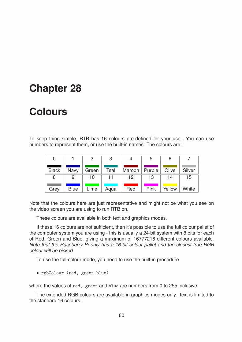
Chapter 28
Colours
To keep thing simple, RTB has 16 colours pre-defined for your use. You can usenumbers to represent them, or use the built-in names. The colours are:
0 1 2 3 4 5 6 7
Black Navy Green Teal Maroon Purple Olive Silver
8 9 10 11 12 13 14 15
Grey Blue Lime Aqua Red Pink Yellow White
Note that the colours here are just representative and might not be what you see onthe video screen you are using to run RTB on.
These colours are available in both text and graphics modes.
If these 16 colours are not sufficient, then it’s possible to use the full colour pallet ofthe computer system you are using - this is usually a 24-bit system with 8 bits for eachof Red, Green and Blue, giving a maximum of 16777216 different colours available.Note that the Raspberry Pi only has a 16-bit colour pallet and the closest true RGB
colour will be picked
To use the full-colour mode, you need to use the built-in procedure
• rgbColour (red, green blue)
where the values of red, green and blue are numbers from 0 to 255 inclusive.
The extended RGB colours are available in graphics modes only. Text is limited tothe standard 16 colours.
80
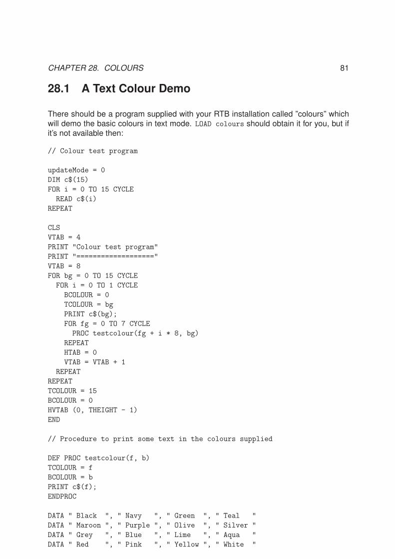
CHAPTER 28. COLOURS 81
28.1 A Text Colour Demo
There should be a program supplied with your RTB installation called ”colours” whichwill demo the basic colours in text mode. LOAD colours should obtain it for you, but ifit’s not available then:
// Colour test program
updateMode = 0
DIM c$(15)
FOR i = 0 TO 15 CYCLE
READ c$(i)
REPEAT
CLS
VTAB = 4
PRINT "Colour test program"
PRINT "==================="
VTAB = 8
FOR bg = 0 TO 15 CYCLE
FOR i = 0 TO 1 CYCLE
BCOLOUR = 0
TCOLOUR = bg
PRINT c$(bg);
FOR fg = 0 TO 7 CYCLE
PROC testcolour(fg + i * 8, bg)
REPEAT
HTAB = 0
VTAB = VTAB + 1
REPEAT
REPEAT
TCOLOUR = 15
BCOLOUR = 0
HVTAB (0, THEIGHT - 1)
END
// Procedure to print some text in the colours supplied
DEF PROC testcolour(f, b)
TCOLOUR = f
BCOLOUR = b
PRINT c$(f);
ENDPROC
DATA " Black ", " Navy ", " Green ", " Teal "
DATA " Maroon ", " Purple ", " Olive ", " Silver "
DATA " Grey ", " Blue ", " Lime ", " Aqua "
DATA " Red ", " Pink ", " Yellow ", " White "
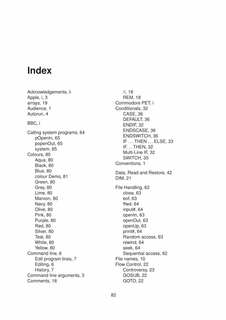
Index
Acknowledgements, iiApple, i, 3arrays, 19Audience, 1Autorun, 4
BBC, i
Calling system programs, 64pOpenIn, 65popenOut, 65system, 65
Colours, 80Aqua, 80Black, 80Blue, 80colour Demo, 81Green, 80Grey, 80Lime, 80Maroon, 80Navy, 80Olive, 80Pink, 80Purple, 80Red, 80Silver, 80Teal, 80White, 80Yellow, 80
Command line, 6Edit program lines, 7Editing, 6History, 7
Command line arguments, 3Comments, 18
//, 18REM, 18
Commodore PET, iConditionals, 32
CASE, 36DEFAULT, 36ENDIF, 32ENDSCASE, 36ENDSWITCH, 36IF . . . THEN . . . ELSE, 33IF. . . THEN, 32Multi-Line IF, 32SWITCH, 35
Conventions, 1
Data, Read and Restore, 42DIM, 21
File Handling, 62close, 63eof, 63ffwd, 64input#, 64openIn, 63openOut, 63openUp, 63print#, 64Random access, 63rewind, 64seek, 64Sequential access, 62
File names, 10Flow Control, 22
Controversy, 23GOSUB, 22GOTO, 22
82
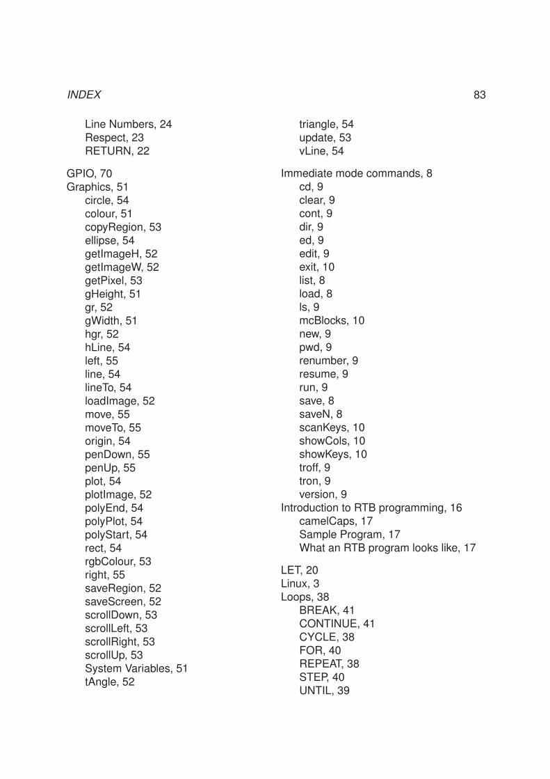
INDEX 83
Line Numbers, 24Respect, 23RETURN, 22
GPIO, 70Graphics, 51
circle, 54colour, 51copyRegion, 53ellipse, 54getImageH, 52getImageW, 52getPixel, 53gHeight, 51gr, 52gWidth, 51hgr, 52hLine, 54left, 55line, 54lineTo, 54loadImage, 52move, 55moveTo, 55origin, 54penDown, 55penUp, 55plot, 54plotImage, 52polyEnd, 54polyPlot, 54polyStart, 54rect, 54rgbColour, 53right, 55saveRegion, 52saveScreen, 52scrollDown, 53scrollLeft, 53scrollRight, 53scrollUp, 53System Variables, 51tAngle, 52
triangle, 54update, 53vLine, 54
Immediate mode commands, 8cd, 9clear, 9cont, 9dir, 9ed, 9edit, 9exit, 10list, 8load, 8ls, 9mcBlocks, 10new, 9pwd, 9renumber, 9resume, 9run, 9save, 8saveN, 8scanKeys, 10showCols, 10showKeys, 10troff, 9tron, 9version, 9
Introduction to RTB programming, 16camelCaps, 17Sample Program, 17What an RTB program looks like, 17
LET, 20Linux, 3Loops, 38
BREAK, 41CONTINUE, 41CYCLE, 38FOR, 40REPEAT, 38STEP, 40UNTIL, 39

INDEX 84
WHILE, 39
Mac, 3Maplin Robot Arm, 73
armBody, 73armElbow, 73armGripper, 73armLight, 73armReset, 73armShoulder, 73armWrist, 73
Matryoshka dolls, 77Minecraft, 68
mcChat, 68mcCircleZ, 69mcConnect, 68mcGetPos, 69mcGetTile, 69mcLine, 69mcSetBlock, 69mcSetBlocks, 69mcSetTile, 69
Miscellaneous Program instructions, 45END, 45STOP, 45SWAP, 45wait, 45
Mouse, 58getMouse, 58mouseOff, 58mouseOn, 58setMouse, 58
Music, 59loadMusic, 59pauseMusic, 59playMusic, 59resumeMusic, 59setMusicVol, 59stopMusic, 59
nano, 11notepad, 11Numbers, 19Numeric Operators, 20
Numerical Functions and data, 46ABS, 47ACOS, 47ASC, 48ASIN, 47ATAN, 47CLOCK, 47COS, 47DEG, 46EXP, 47HASH, 47INT, 47LEN, 48LOG, 47MAX, 47MIN, 47PI, 46PI2, 46RAD, 47RND, 47SEED, 46SGN, 47SIN, 47SQRT, 47System variables and constants, 46TAN, 47TIME, 46VAL, 48
PC, 3Precedence, 20Preface, iprint, 30Prompt, 5
Raspberry Pi, 3Raspberry Pi GPIO, 70
analogRead, 71analogWrite, 71Constants, 70digitalRead, 71digitalWrite, 71Instructions, 71pinInput, 70
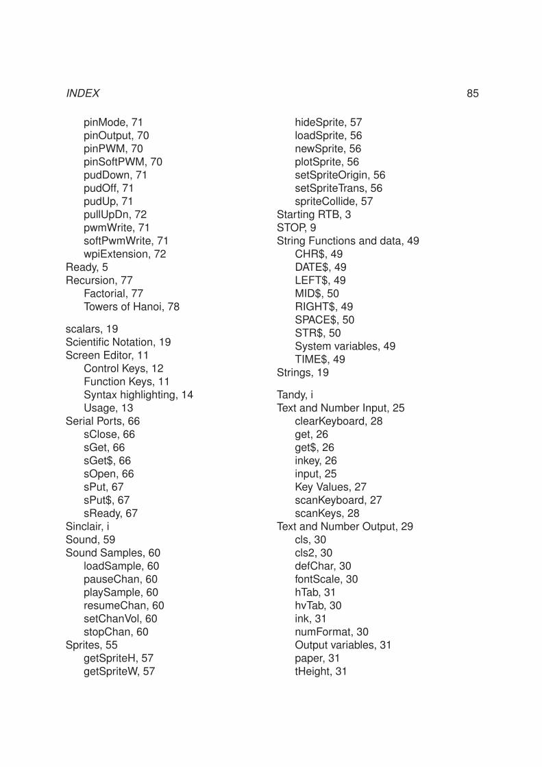
INDEX 85
pinMode, 71pinOutput, 70pinPWM, 70pinSoftPWM, 70pudDown, 71pudOff, 71pudUp, 71pullUpDn, 72pwmWrite, 71softPwmWrite, 71wpiExtension, 72
Ready, 5Recursion, 77
Factorial, 77Towers of Hanoi, 78
scalars, 19Scientific Notation, 19Screen Editor, 11
Control Keys, 12Function Keys, 11Syntax highlighting, 14Usage, 13
Serial Ports, 66sClose, 66sGet, 66sGet$, 66sOpen, 66sPut, 67sPut$, 67sReady, 67
Sinclair, iSound, 59Sound Samples, 60
loadSample, 60pauseChan, 60playSample, 60resumeChan, 60setChanVol, 60stopChan, 60
Sprites, 55getSpriteH, 57getSpriteW, 57
hideSprite, 57loadSprite, 56newSprite, 56plotSprite, 56setSpriteOrigin, 56setSpriteTrans, 56spriteCollide, 57
Starting RTB, 3STOP, 9String Functions and data, 49
CHR$, 49DATE$, 49LEFT$, 49MID$, 50RIGHT$, 49SPACE$, 50STR$, 50System variables, 49TIME$, 49
Strings, 19
Tandy, iText and Number Input, 25
clearKeyboard, 28get, 26get$, 26inkey, 26input, 25Key Values, 27scanKeyboard, 27scanKeys, 28
Text and Number Output, 29cls, 30cls2, 30defChar, 30fontScale, 30hTab, 31hvTab, 30ink, 31numFormat, 30Output variables, 31paper, 31tHeight, 31

INDEX 86
tWidth, 31vTab, 31
Tones and Sounds, 60envelope, 61sound, 61tone, 60
Trademarks, iiTRS-80, i
updateMode, 29User defined Procedures and Functions,
75=, 76def proc, 75Functions, 76proc, 76Procedures, 75
Variables, 19Arrays, 21Assignment, 20Associative Arrays, 21Map, 21Names, 19Scope, 78Types, 19
vim, 11
Warning, 2