1

Retail Store Execution: An Empirical Study1

Marshall L. Fisher Jayanth Krishnan Serguei Netessine

Operations and Information Management Department

The Wharton School, University of Pennsylvania [fisher, jayanth, netessine]@wharton.upenn.edu

December 2006

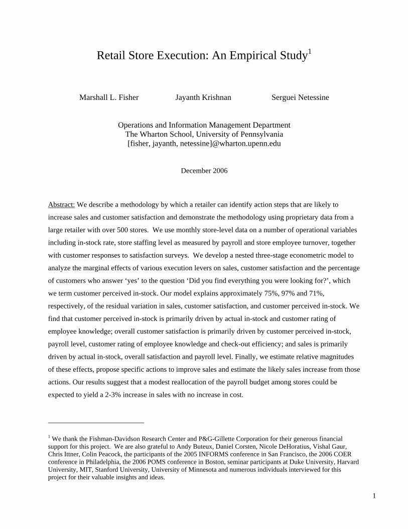
Abstract: We describe a methodology by which a retailer can identify action steps that are likely to

increase sales and customer satisfaction and demonstrate the methodology using proprietary data from a

large retailer with over 500 stores. We use monthly store-level data on a number of operational variables

including in-stock rate, store staffing level as measured by payroll and store employee turnover, together

with customer responses to satisfaction surveys. We develop a nested three-stage econometric model to

analyze the marginal effects of various execution levers on sales, customer satisfaction and the percentage

of customers who answer ‘yes’ to the question ‘Did you find everything you were looking for?’, which

we term customer perceived in-stock. Our model explains approximately 75%, 97% and 71%,

respectively, of the residual variation in sales, customer satisfaction, and customer perceived in-stock. We

find that customer perceived in-stock is primarily driven by actual in-stock and customer rating of

employee knowledge; overall customer satisfaction is primarily driven by customer perceived in-stock,

payroll level, customer rating of employee knowledge and check-out efficiency; and sales is primarily

driven by actual in-stock, overall satisfaction and payroll level. Finally, we estimate relative magnitudes

of these effects, propose specific actions to improve sales and estimate the likely sales increase from those

actions. Our results suggest that a modest reallocation of the payroll budget among stores could be

expected to yield a 2-3% increase in sales with no increase in cost.

1 We thank the Fishman-Davidson Research Center and P&G-Gillette Corporation for their generous financial support for this project. We are also grateful to Andy Buteux, Daniel Corsten, Nicole DeHoratius, Vishal Gaur, Chris Ittner, Colin Peacock, the participants of the 2005 INFORMS conference in San Francisco, the 2006 COER conference in Philadelphia, the 2006 POMS conference in Boston, seminar participants at Duke University, Harvard University, MIT, Stanford University, University of Minnesota and numerous individuals interviewed for this project for their valuable insights and ideas.

2

1. Introduction

It is sometimes said that success is the result of a good plan well executed. For a retailer, plans

are mostly formulated at corporate headquarter and executed in their stores. Corporate planning functions

include choosing the assortment of products to carry in each store at each point in time, setting store

inventory levels and product prices, setting staffing levels, determining how many stores to have and

where they are located and creating the physical design of stores and planograms that specify the location

of all products within each store.

A retail store is an interesting amalgam of a factory and a sales office and store employees are

responsible for a wide range of execution tasks that collectively determine the success of corporate plans.

Factory related store execution tasks include receiving product, moving product from the back room to

shelves as needed, putting items moved by a customer back to where they belong on the shelf and

checking customers out. Fisher (2004) notes similarities between the execution tasks of a retail store and

an automobile assembly plant, and suggests drawing on the Toyota Production System as a source of

ideas for improving retail store execution. Sales office store execution tasks include all interactions with

customers, such as greeting them, asking if they need help, and when requested, providing advice to

enable them make a purchase decision and to find the products they have decided to buy.

Academic research to date has focused almost exclusively on planning functions. For example,

the operations management literature includes numerous papers on inventory optimization that are

applicable to setting planned inventory levels in a retail store. Recently, however, a few pioneering papers

(Raman et al. 2001a, 2001b, DeHoratius and Raman 2003, Ton and Raman 2004, Corsten and Gruen

2003, Ton and Huckman 2005, Van Donselaar et al. 2006) have provided evidence of deficiencies in

retail store execution, suggesting that optimized plans might be severely blunted by less than perfect

execution. Although these papers have focused mostly on missing inventory, inventory record inaccuracy

and inventory replenishment, it is reasonable to suspect that, given the high level of problems with

inventories, other aspects of retail execution are imperfect also.

Interestingly, for many years, retailers have been administering surveys to their customers to

measure both their overall level of satisfaction and their opinion of various details of their store

experience. Many of the detailed questions relate to store execution. For example, ‘Did you find what you

were looking for?’ is a commonly asked question directly related to the missing inventory issue noted

above. It is thus natural to consider using this data to better understand issues related to store execution,

including what factors influence the quality of execution and what is the impact of execution on output

variables of interest to the retailer, such as sales and overall customer satisfaction. This paper reports an

3

effort to do this using proprietary data obtained from a large retail chain with over 500 stores. The data is

tracked monthly at the store level for a 17 month period and is comprised of 1) financial store

performance data, including sales, number of transactions and number of units sold, 2) operational data,

such as payroll, employee turnover, and in-stock levels, and 3) the results of ongoing customer

satisfaction surveys that use a variety of questions to measure for a particular store visit a customer’s

overall satisfaction as well as their perception of various aspects of their experience that may have

influenced their overall satisfaction.

We analyzed this data to discern correlates of 1) sales, 2) overall customer satisfaction and 3) the

percentage of customers who answered ‘yes’ to the question ‘Did you find everything you were looking

for?’, a metric we call customer perceived in-stock. Because we were interested in assessing the impact

of the detailed variables on sales, satisfaction and customer perceived in-stock, we first transformed the

data to attempt to remove spurious sources of correlation. For example, most variables were impacted by

time, via trend and seasonality, and hence might be correlated with each other because of this common

correlation with time, but this type of correlation was not of interest to us. We thus applied a data

transformation procedure that (1) removes seasonality, (2) de-trends the data to control for store openings

and economic trends, (3) removes forward-looking components from the data by accounting for

managerial decisions that are based on the sales forecast, (4) controls for autoregressive properties and (5)

standardizes the data to control for store heterogeneity. We then pooled this data panel and analyzed it

using a nested three-stage model that explains the direct and indirect drivers of sales, overall customer

satisfaction, and customer perceived product availability.

Our model explains approximately 75%, 97% and 71% of transformed data’s variations in,

respectively, sales, overall customer satisfaction, and customer perceived product availability. We find

that customer perceived in-stock is primarily driven by actual in-stock and customer rating of employee

knowledge; overall customer satisfaction is primarily driven by customer perceived in-stock, payroll

level, customer rating of employee knowledge and check-out efficiency; and sales is primarily driven by

actual in-stock, overall satisfaction and payroll level.

We observe that stores within the chain vary greatly in their responsiveness to changes in

controllable variables. For example, we find that increasing associate payroll by $1 at a given store is

associated with a sales lift of anywhere from $4 to $28, depending on the current level of payroll relative

to store sales. The implication of this finding on retail performance is quite dramatic. We show that a

modest reallocation of payroll from stores with low sales lift to stores with high sales lift could be

expected to yield a 2.6% sales lift at no additional cost, a level of sales increase that is large relative to

year to year changes in sales for mature stores.

The primary contribution of this paper is a methodology to help a retailer identify action steps

4

that can increase sales, customer satisfaction and store execution. Although we designed this

methodology to fit the specific data set that was available to us, we believe that it can be adapted to match

the needs of other retailers. Our second contribution is to suggest, based on one retailer, findings about

store execution that might apply to other retailers. While our findings are based on a data set whose

extensiveness and richness are rarely, if ever, found in the literature, given that this data comes from a

single retailer, we are uncertain of the extent to which our findings about drivers of sales and satisfaction

would hold true for other retailers. We hope this study will stimulate additional research with other

retailers, so as to identify common factors driving excellent execution.

The remainder of this paper is organized as follows. Section 2 surveys relevant literature, Section

3 describes our data set, Section 4 presents the transformation we performed on data prior to analysis and

Section 5 describes our analysis and the resulting model. In section 6 we discuss our technical findings

and in Section 7 we describe some managerial implications of our results.

2. Literature Review

Our research agenda on retail store execution straddles three existing areas of literature: 1)

empirical studies of retail store execution, 2) literature on the relationship between customer satisfaction

and financial performance in the retail industry and 3) empirical studies of execution in other industries

such as retail banking and automotive manufacturing.

Retail store execution strategies have attracted the attention of researchers in operations

management only recently, but this stream of work is most closely related to our paper. Perhaps the first

reference on retail store execution is Salmon (1989) who argued that execution in retailing has become

more important than other aspects of retail business (e.g., merchandising). DeHoratius and Raman (2006)

analyze the relationship between incentives provided to store managers and monthly sales and shrinkage

across a chain of stores. They control for store fixed effects, inventory, and advertising expenditures and,

as in our work, find a positive and significant relationship between inventory and sales at the store level.

The literature on missing inventory and inventory record inaccuracy in retailing (see Raman et al. 2001a,

2001b) found empirically that, because of execution failures, customers often do not find the products

they seek, even if these products are within the store. Raman et al. (2001a, 2001b) report that over 65%

of the inventory records at retailer Gamma were inaccurate at the store-SKU level, and that over 16% of

the inventory at retailer Beta was missing from the shelf. Their studies report that such issues arise

mainly due to store and distribution center replenishment processes, merchandising, inventory

management and employee turnover. DeHoratius and Raman (2003) outline three approaches to the

inaccurate inventory problem: prevention and elimination of root causes (using methods similar to the

5

Ishikawa process of JIT principles), correction and identification of errors through inspection policies,

and lastly software solutions that integrate the source of errors into the inventory management system. In

a follow-up study, Ton and Raman (2004) find that higher product variety and inventories lead to a higher

incidence of phantom stockouts (such that inventory is in the back room but does not reach the shelf) and

lost sales. Ton and Huckman (2005) study the impact of employee turnover on process conformance

within retail stores and find that the negative effect of turnover is most pronounced in stores with low

process conformance (lesser discipline in process execution and adherence to quality standards). Corsten

and Gruen (2003) study the root causes of retail inventory stockouts and point to mechanisms that address

the issue of stockouts and improve sales. Van Donselaar et al. (2006) find that store managers

systematically made corrections on automated order advices either by shifting orders from peak days to

non-peak days or by changing the order size. Fundamentally, this stream of literature has viewed retail

operation from the factory lens while omitting the service delivery and customer-employee interaction

aspects of retailing. For example, Fisher (2004) argues that both the auto plant and a retail store face a

similar execution challenge of making sure what is needed arrives at the right time.

Literature on customer satisfaction is voluminous and spans several areas such as marketing,

management and accounting. For example, numerous papers use the ACSI (American Customer

Satisfaction Index) to study customer satisfaction at the company, industry and macroeconomic levels.

For the purposes of our paper, we focus only on customer satisfaction studies that are immediately related

to our work in retailing and do not survey the literature that studies the design of satisfaction survey

instruments, because in this work we had no control over survey design. The basic tenet of this research

stream is that higher service quality improves customer satisfaction, resulting in better financial

performance, although the mechanisms by which this improvement happens vary. Iacobucci et al. (1994,

1995) provide precise definitions of service quality versus customer satisfaction. They contend that

service quality should not be confused with customer satisfaction, but that satisfaction is a positive

outcome of providing good service. Ittner and Larcker (1998) provide empirical evidence at the

customer, business-unit and firm- level that various measures of financial performance (including

revenue, revenue change, margins, return on sales, market value of equity and current earnings) are

positively associated with customer satisfaction. However, in the retail industry they find a negative

relationship between satisfaction and profitability which may be because benefits from increased

satisfaction can be exceeded by the incremental cost in retail. Sulek et al. (1995) find that customer

satisfaction positively affects sales per labor hour at a chain of 46 retail stores. Anderson et al. (2004)

find a positive association between customer satisfaction at the company level and Tobin’s q (a long-run

measure of financial performance) for department stores and supermarkets. Babakus et al. (2004) link

customer satisfaction to product and service quality within retail stores and find that product quality has a

6

significant impact on store-level profits. To summarize, research on customer satisfaction views

employees as facilitators of the sales process who are critical to improving the conversion ratio, by

providing information to the customers on prices, brands, and product features and by helping customers

to navigate store aisles, finding the product and even cross-selling other products. The unique feature of

the retail store execution problem is that it combines the factory and the sales components, but this stream

of literature focuses only on the latter.

Empirical studies of execution span other industries as well. For example, retail banking is

dominated by the sales function; Frei and Harker (1999) quantify the inefficiencies in process execution

due to process design using Data Envelopment Analysis. Frei et al. (1999) study the impact of the

aggregate process performance and process variation on the financial outcome using a sample of 135

bank branches. They report that process variation negatively affects financial performance. Another

prominent focus on execution which takes the factory viewpoint is found in the automotive industry. In

this context the role of process design and conformance has long been debated, and the virtues of the

Toyota Production System are well documented. Womack et al. (1991) show that Toyota’s competitive

advantage arises from a combination of employee motivation, training, process designs and JIT

techniques. Fisher and Ittner (1999) study the impact of product variety on automotive assembly plant

operations and find that increased option content variability in car assembly has an adverse effect on

plants’ operational performance, which is manifested in higher total labor hours, overhead hours,

downtime hours, rework and inventory levels. MacDuffie et al. (1996) find that parts complexity

persistently impairs productivity.

Perhaps the closest to retailing are the streams of literatures studying customer satisfaction,

operational failures and performance in the airline and healthcare industry, because these industries too

combine factory and sales components of execution. Studies of execution in the healthcare industry

focused on operational failures in the execution process (Tucker 2004) as well as on learning through

these failures (Tucker and Edmondson 2003). Ren and Wang (2006a) empirically link process

consistency and service quality while Ren and Wang (2006b) further show how service quality affects

volume at US hospitals. Using data on customer complaints caused by operational failures in the airline

industry, Lapre and Tsikriktsis (2006) find that customer dissatisfaction follows a U-shaped function of

operating experience: first dissatisfaction decreases with experience because airlines learn but then

dissatisfaction increases because customers increase their expectations of service. Tsikriktsis (2006)

shows that the relationship between operational performance and profitability depends upon a company’s

operating model; “focused” airlines show a link between late arrivals and profitability, whereas full-

service airlines do not. Moreover, capacity utilization is a stronger driver of profitability for full-service

airlines than for focused airlines. Anderson et al. (2006) find that drivers of customer satisfaction are

7

affected by customer attributions of blame for service failures: namely, customer-employee interactions

are less important when the customer attributes blame to the service provider.

3. Data Description

Our study requires detailed store-level and customer survey data which is not publicly available.

To obtain these data we worked closely with a large national retail chain under conditions of anonymity

and nondisclosure. Therefore, we are unable to reveal either the name of the retailer, or provide details on

its product lines and retail segment. The data comes from more than 500 stores over a period spanning 29

months. The retailer operated its stores centrally so that the headquarters planned the assortment, prices,

payroll and employee training. The store manager had the authority to hire and terminate employees

using a planned payroll budget for the month as a guideline. The store manager’s compensation was not

contingent on monthly sales at the store. The retailer did not tailor product assortments to customer

demographics or store size.

We obtained two types of data: financial and operational data collected by the retailer and the

results of a customer survey administered by an independent company on the retailer’s behalf. Financial

and operational data were available for the 29-month period and customer survey data were available for

four years. Since we did not have financial and operational data for a significant part of this period, we

eliminated surveys that did not have matching store-level data. Moreover, customer surveys changed

significantly over time, with the number of questions in each month ranging from about 10 to about 70.

Answer scales varied over the years as well. To overcome this problem, we decided to focus only on 13

key questions that remained unchanged over a 17-month period and that, we believe, are most closely

related to store execution policies. Thus, we limit our study to 17 months starting from January 2004.

We summarize corresponding variables in Table 1 where we calculate descriptive statistics for each

variable across stores over the period of study.

Financial and operational data

We use subscript i to denote stores which range from 1 to 437 and we use subscript t to denote

time periods from 1 to 17. We note that new store openings were quite common over the study period

and naturally these new stores have many missing observations.

SALES, TRANSACTIONS and UNITS.SOLD denote, respectively, monthly sales in $, monthly

number of instances in which customers bought something in the store and monthly unit sales. Stores

averaged $436,032 in monthly sales but varied significantly (from $77,000 to $1,400,000). On average,

there were 10,019 transactions and 34,035 unit sales per month per store indicating an average basket size

of $44 (SALES/TRANSACTIONS), approximately 3.4 (UNITS.SOLD/TRANSACTIONS) products per

8

basket and approximately $13 (SALES/UNITS.SOLD) average sales per product.

CLEARANCE is the dollar value of all products that were marked down and sold on clearance in

a given month (not including advertised promotions or markdowns planned by the central office across

the entire chain). An average store sold only about $2,000 worth of merchandise per month on clearance.

Store managers had discretion over which items went on clearance. We note that the maximum value for

CLEARANCE is 7 times higher than the average value, indicating wide dispersion in the enactment of

this practice relative to SALES where the maximum is only about three times higher than the mean.

Clearly, CLEARANCE is only a proxy for a store manager’s action to put products on clearance sales

because we only know the amount that was actually sold.

OVERRIDE is the dollar value for all sales that required a managerial override. A managerial

override happens at the discretion of the store manager, when the customer reports a damaged product or

a wrong price sticker, at which point the manager may decide to override the price recorded in the system.

On average, only about $1,000 worth of merchandise in a given month required managerial override.

Similar to CLEARANCE, there is a wide dispersion in OVERRIDE across stores (in that the maximum

value is 9 times higher than the average value).

RETURN is the dollar value of all products that were returned per month and for which money

was refunded to the customer. Returns might be reflective of store execution policies, because they are

often caused by the lack of communication between customers and employees regarding product features.

On average, a store had $73,000 dollars of merchandise returned, or about 17% of sales. Variation in this

variable is similar to variation in SALES in that the maximum value is about three times the average.

MOS (marked out of stock) is the dollar value of all items that customers found in the store, but

which the store’s computer showed as out of stock. On average, only about $8,000 worth of merchandise

was marked out of stock in a given month, but this number varied somewhat from store to store (the

maximum value of MOS is 4.5 times the average). Note that MOS can be viewed as a proxy for

inventory record inaccuracy although it does not account for cases in which the item is in the computer

system but is not in the store and it only accounts for situations in which customers “correct” the

inaccuracy. Clearly, overall inventory record inaccuracy can be much higher.

ASSOCIATE.PLAN.DOLLARS and MANAGER.PLAN.DOLLARS are payroll budgets for

each store for a given month. Payroll budgets are based on the expectation of sales in a given month. On

average, a store planned to pay $23,657 per month to associates and $20,047 to managers per month

which, in total, amounts to about 10% of sales.

ASSOCIATE.DOLLARS and MANAGER.DOLLARS are actual payrolls for store associates

and managers in a given month. The store manager can deviate from the store payroll budget based on

the number of new terminations, absenteeism and immediate needs. Thus, both random events and the

9

store manager’s decisions cause deviations. For example, if absenteeism is higher in a given month, the

manager might end up spending less money on payroll than anticipated. On average, it appears that the

actual payroll for associates is slightly higher than the planned payroll, but that the actual payroll for

managers is somewhat lower than the planned payroll.

ASSOCIATE.TERMINATIONS and MANAGER.TERMINATIONS are the number of

terminations at the associate and managerial levels, respectively. On average, 1.56 associates (which is

equivalent to 6%) and only 0.11 managers (which is equivalent to 1.9%) were terminated (voluntarily or

involuntarily) per month. These two variables are measures of turnover within the store, which may

affect store execution processes and customer satisfaction due to a lack of experience and knowledge

continuity among new employees (Ton and Huckman 2005).

ESTIMATED.INSTOCK is the percentage of SKUs in stock at the end of the month. Such

measure of inventory availability is quite standard in retail practice and we use ESTIMATED.INSTOCK

as a proxy for physical inventory availability. Average ESTIMATED.INSTOCK for all stores was 93%.

Customer survey data

The retail chain administered automated customer surveys over the phone. When customers paid

their bill at the checkout, they were randomly chosen to answer a satisfaction survey. The point-of-sales

terminal then printed an invitation to call a toll-free number to answer a series of questions using the

numeric pad on the telephone; customers were entered into a lottery with a cash prize as a reward for

participating in this survey. We obtained customer surveys over a four-year period, with the number of

responses varying from 10,000 to 30,000 per month for the entire chain and constituting approximately

0.5% of all customer transactions. Among 13 questions we focus on, most had “yes-no” (with 1 for yes

and 0 for no) answers, except for those questions whose answers are indicated by the variables

KNOWPRODUCT, KNOWBRANDS, KNOWPRICES and OVERALLRATING, all of which were

rated on a 10-point Likert scale. Since this data is at the customer level, we use the time of visit and the

store number reflected on every response to associate each response with a store-month combination. For

yes/no questions we calculate the fraction of “yes” answers for each store-month combinations. For all

other questions we calculate the equally-weighted response value for each store-month.

AISLEDEBRIS indicates the percentage of customers who found debris in store aisles. On

average, customers experienced obstruction in aisles 18% of the time, but there was significant variability

(from 5% to 55%).

GREETING is percentage of customers who were greeted in the store. On average, customers

were greeted 73% of the time.

ASSTNEEDED is the percentage of customers who needed assistance, but were unable to find it.

10

Customers could not find assistance 14% of the time, on average.

CHECKOUT is the percentage of customers who found the checkout to be quick and efficient.

On average, the checkout process was efficient 90% of the time, with some variability (78% to 98%).

BEYONDREACH is the percentage of customers who were interested in purchasing a product,

but found the product too high or too deep on the shelves. Customers could not reach for the item in 19%

of the cases, on average.

CUSTOMER.INSTOCK is the percentage of customers who found everything that they were

looking for in the store. We use this variable to measure customers’ perception of in-stock, which

averaged 76% for the entire chain. Since the question asked customers about their entire shopping basket,

finding that even one out of several products was out of stock would trigger a “No” response to this

question. Since an average basket had about 3.4 items, the answer to this question is quite close to what

we would expect, given 93% average ESTIMATED.INSTOCK (0.933.4=0.75). Thus, we do not have

evidence of significant phantom stockouts (Raman et al. 2001). However, it is possible that some

customers simply left the store without buying anything (and hence did not respond to the survey)

because they were unable to find products.

FINDINGPRICE is the percentage of customers who had difficulty finding the price of a product.

On average, 15% of customers experienced this difficulty.

KNOWPRODUCTS, KNOWBRANDS and KNOWPRICES are indicators of how

knowledgeable employees were with respect to products, brands and prices, respectively. Summary

statistics indicate that all three of these ratings were generally between 7 and 9, on average.

WILLRETURN is the percentage of customers who said they will return to the store. On

average, 99% of customers were planning to return to the store. This number had little variability (95% to

100%).

VALUE is the percentage of customers who thought that they got their value for the money. On

average, 93% of customers believed that their value for money was adequate. This number had little

variability (89% to 98%).

OVERALL.RATING is the average customer satisfaction rating for the store on a particular visit

relative to expectations. Average chain-wide satisfaction was 8.4 on a 10-point scale and varied from 7.9

to 9.17, on average. For comparison, Morgan and Rego (2006) find that average customer satisfaction in

the US economy is 7.8 on the same scale.

Our data comes with several limitations. Ideally, we would like to use profit at the store level as a

measure of financial performance, but this particular retailer tracked profit only at the chain level.

Moreover, this retailer believed that store employees primary impact was on sales. This is because most

decisions that would impact cost, including the level of inventory, the price paid for products, store

11

employee payroll and the quality of store fixtures, were made centrally at corporate headquarters.

Furthermore, we do not have customer-level data on the number of purchases by each customer in a

month. Thus, we acknowledge the possibility that customers who shop often at the store may skew the

results of the satisfaction survey because they respond more often (although the survey does ask

customers to evaluate their experience on a particular visit, not their average experience, and therefore

this bias may not be significant). We also do not have data on the number of customers who did not visit

the store because they were dissatisfied or the number of customers who did visit the store but left without

buying. These customers do not respond to the satisfaction survey and hence their absence might

introduce additional biases. Overall, it would be helpful to supplement customer questionnaires with the

results of independent audits, but this particular chain did not conduct such audits. The retailer also did

not track other variables that could potentially help us better understand in-store operating policies. For

example, we were unable to obtain data on the exact extent of compliance with store policies (e.g., the

store manager’s adherence to the planogram), shrink, etc. However, we made every attempt to obtain as

much data as the retailer collected. Likewise, our data from the customer satisfaction survey is driven by

data availability, since we did not participate in the survey design. That said, our analysis relies on a data

set whose extensiveness and richness are rarely, if ever, found in the literature. The final data set we

analyzed contained 6310 store-month data points for 437 stores over 17 months for which we have

matching operational/financial data as well as results of customer surveys.

4. Data Transformation

We conducted exploratory analyses and questioned company employees regarding exact data

collection procedures and the nature of their business. Further, we conducted preliminary data analysis

by calculating descriptive statistics and pair-wise correlations. Based on this exploratory analysis, we

eliminated several variables from our analysis. First, we determined that TRANSACTIONS and

UNITS.SOLD are highly correlated with SALES (with pair-wise correlations more than .99). Hence, for

the remainder of the paper, we focus only on SALES as our measure of financial performance. We

repeated our analysis using the two other variables as measures of financial performance, and results were

qualitatively the same. Furthermore, we determined that product returns did not vary significantly by

store: in fact, we found that the RETURN variable is highly correlated (correlation >.99) with SALES,

indicating that this number might be reflective of the nature of the product line itself rather than processes

within the store. We therefore omit this variable from the analysis.

Among customer survey variables, we found that KNOWPRODUCTS, KNOWBRANDS and

KNOWPRICES were all highly correlated (pair-wise correlations >.95), so we combine them into a

single TOTKNOWLEDGE variable using equal weights (Kennedy 2003). Finally, we established that

12

OVERALL.RATING is highly correlated with the variables WILLRETURN and VALUE (pair-wise

correlations >.9). Thus, in the remainder of our analysis, we use only OVERALL.RATING as an overall

measure of customer satisfaction which is in line with Morgan and Rego (2006) who found that average

satisfaction scores have the greatest value in predicting financial performance. Moreover, we did not use

WILLRETURN, because customers who live in close proximity to the store might return to the store even

if they are unsatisfied. We did not use VALUE because it relies, in large part, on how reasonably priced

the products in the store are, something that is beyond the control of the store manager. As a robustness

check, we also attempted to use an equally weighted combination of all three of these measures, and

results were qualitatively the same.

Even after eliminating these variables, we discovered that the data possessed several features that

complicated analysis: it was seasonal; stores exhibited sales trends; some variables were endogenously

codetermined (e.g., payroll was based on expected sales but sales were also a function of payroll) and

others possessed autoregressive properties (e.g., satisfaction in the current month affected sales both for

current and future months); and stores exhibited significant cross-sectional heterogeneity (e.g., in sales

levels). In this section we describe the data transformation procedure we have employed to convert the

raw data so as to control for all of these effects. The ultimate goal is to obtain the data set that would

allow us to analyze “within-month” changes in the dependent variable (sales) and all independent

variables that are devoid of long-term effects (e.g., seasonality, trends) and do not incorporate

expectations for the future. Without this data transformation, we might observe effects due to a different

mechanism than we seek to understand which would not allow us to discern the true causal mechanisms

(e.g., how operational policies drive sales and satisfaction).

Seasonality

It is well-documented that retailers experience significant seasonality in sales (see Fisher et al.

2000), and consequently their staffing and inventory management decisions are subject to seasonal effects

as well. Hence, some variables may exhibit a spurious correlation over time due to seasonality, which

would confound the true relationship between them. Using exploratory analysis, we noticed that even

variables such as customer satisfaction exhibited strong seasonality. Therefore we de-seasonalize all

variables in the data. We use a multiplicative model of seasonality and estimate seasonal coefficients

endogenously using chain-wide data for all stores and all months. Thus, we ignore seasonal differences

among stores (because the sale of this particular merchandise is not strongly affected by geographical

location but is strongly affected by holiday sales patterns) and we use data for each variable separately

(e.g., we de-seasonalize sales using sales data and customer satisfaction using customer satisfaction data).

In our data seasonality alone explained 45% of chain-wide variations in sales. Since results of the

13

customer satisfaction survey were confined to 17 months only, we used responses to the

OVERALL.RATING question to de-seasonalize all customer satisfaction data, because responses to this

question were available for a 29-month period coinciding with the availability of operational data.

Moreover, from the limited data that we had it appeared that seasonal patterns are similar among all

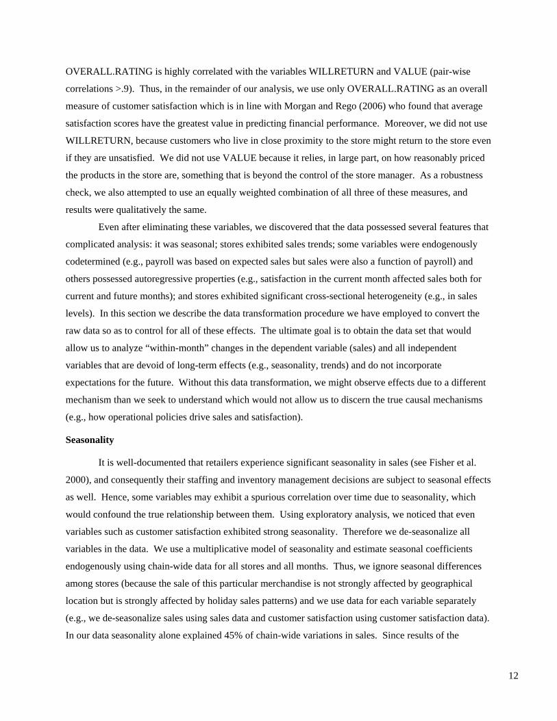
survey variables. The resulting formula is:

( , ) ( , )

/ , ( ),it it i ij j

y y y y m tτ ττ τ

τ⎛ ⎞

= ∀ =⎜ ⎟⎝ ⎠∑ ∑ ,

where ity is any variable in the data set (see Table 1) and ity is the de-seasonalized variable, the subscript

τ ranges from 1 to 12 and denotes the month of the year in which t occurs, and m(t) denotes the month (1

to 12) corresponding to t. We note that sales experiences wide seasonal fluctuations with coefficients

ranging from 0.6 in April to 1.8 in December while satisfaction and in-stock vary less (from 0.8 in April-

December to 1.3 in January-March).

One notable flaw in our approach is that some high-sales events fall on different months in

different years (e.g., Easter falls on March or April). There are several alternative ways to de-seasonalize

the data, although the approach we use is quite standard. We could have de-seasonalized each variable

for each store using only this store’s data but it is not clear how to treat new stores that do not have

enough historical data. We could have used an additive model of seasonality, i.e., it ity y τε= + . This

approach, however, is questionable since sales vary widely by store. We could also de-seasonalize all

variables using sales rather than this variable’s time series. However, we observed in the data that

customer satisfaction exhibits very different seasonality from sales and therefore we could not justify this

approach.

Trends

Long-term trends in the economy (such as changes in incomes, inflation and consumer

preferences) often affect customer purchasing decisions (see Ittner and Larcker 1998). Strategic decisions

such as the entry of a competitor might lead to growth or decay in sales and satisfaction (see Mittal et al.

2005). Additionally, in our data we found that the strongest source of trends was a pattern of sales growth

in the two to three years after a store opened. For example, new stores in our data exhibited dramatic

growth in sales and a decline in customer satisfaction, resulting in a spurious negative correlation between

sales and satisfaction over time. Over the study period, 97 stores were opened and no stores were closed.

To control for these effects, we de-trend each variable separately for each store using the linear trend

model. We then use the error from this de-trending procedure as the de-trended variable as follows:

14

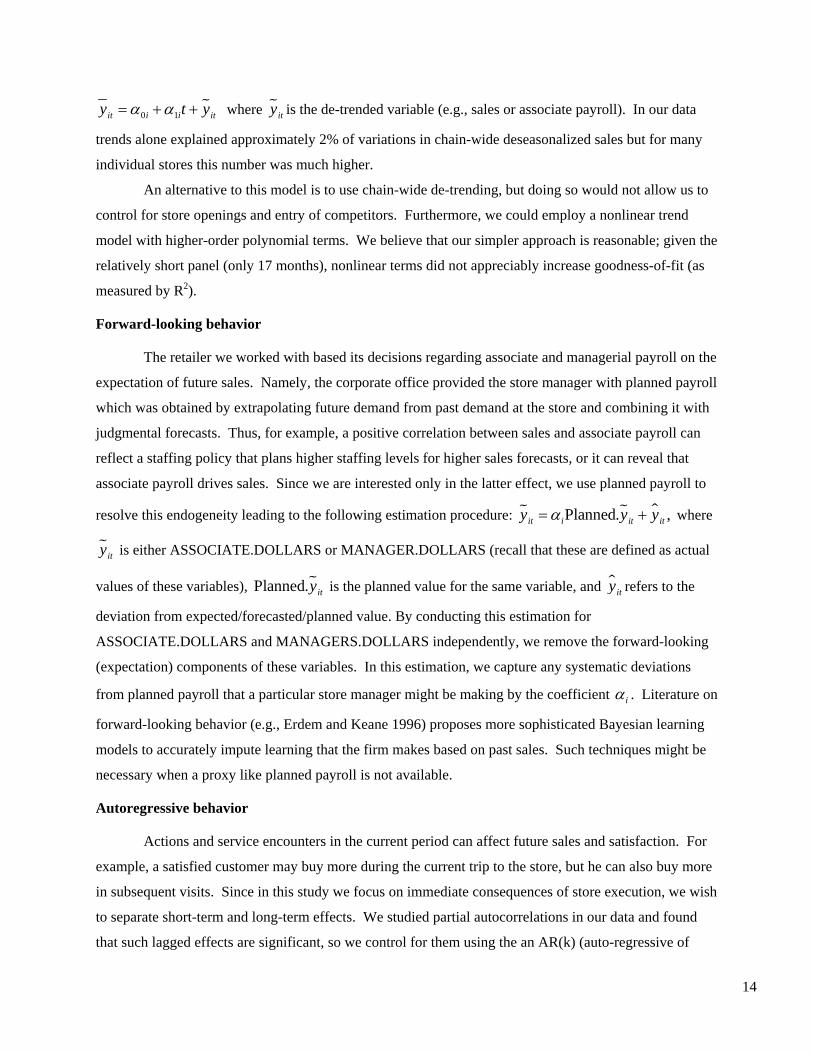
%0 1i iit ity t yα α= + + where % ity is the de-trended variable (e.g., sales or associate payroll). In our data

trends alone explained approximately 2% of variations in chain-wide deseasonalized sales but for many

individual stores this number was much higher.

An alternative to this model is to use chain-wide de-trending, but doing so would not allow us to

control for store openings and entry of competitors. Furthermore, we could employ a nonlinear trend

model with higher-order polynomial terms. We believe that our simpler approach is reasonable; given the

relatively short panel (only 17 months), nonlinear terms did not appreciably increase goodness-of-fit (as

measured by R2).

Forward-looking behavior

The retailer we worked with based its decisions regarding associate and managerial payroll on the

expectation of future sales. Namely, the corporate office provided the store manager with planned payroll

which was obtained by extrapolating future demand from past demand at the store and combining it with

judgmental forecasts. Thus, for example, a positive correlation between sales and associate payroll can

reflect a staffing policy that plans higher staffing levels for higher sales forecasts, or it can reveal that

associate payroll drives sales. Since we are interested only in the latter effect, we use planned payroll to

resolve this endogeneity leading to the following estimation procedure: % % $Planned. ,iit it ity y yα= + where

%ity is either ASSOCIATE.DOLLARS or MANAGER.DOLLARS (recall that these are defined as actual

values of these variables), %Planned. ity is the planned value for the same variable, and $ ity refers to the

deviation from expected/forecasted/planned value. By conducting this estimation for

ASSOCIATE.DOLLARS and MANAGERS.DOLLARS independently, we remove the forward-looking

(expectation) components of these variables. In this estimation, we capture any systematic deviations

from planned payroll that a particular store manager might be making by the coefficient iα . Literature on

forward-looking behavior (e.g., Erdem and Keane 1996) proposes more sophisticated Bayesian learning

models to accurately impute learning that the firm makes based on past sales. Such techniques might be

necessary when a proxy like planned payroll is not available.

Autoregressive behavior

Actions and service encounters in the current period can affect future sales and satisfaction. For

example, a satisfied customer may buy more during the current trip to the store, but he can also buy more

in subsequent visits. Since in this study we focus on immediate consequences of store execution, we wish

to separate short-term and long-term effects. We studied partial autocorrelations in our data and found

that such lagged effects are significant, so we control for them using the an AR(k) (auto-regressive of

15

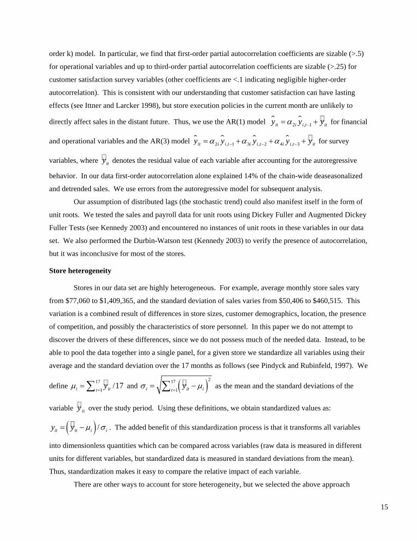
order k) model. In particular, we find that first-order partial autocorrelation coefficients are sizable (>.5)

for operational variables and up to third-order partial autocorrelation coefficients are sizable (>.25) for

customer satisfaction survey variables (other coefficients are <.1 indicating negligible higher-order

autocorrelation). This is consistent with our understanding that customer satisfaction can have lasting

effects (see Ittner and Larcker 1998), but store execution policies in the current month are unlikely to

directly affect sales in the distant future. Thus, we use the AR(1) model $ $2 , 1iit i t ity y yα −= + for financial

and operational variables and the AR(3) model $ $ $ $2 3 4, 1 , 2 , 3i i iit i t i t i t ity y y y yα α α− − −= + + + for survey

variables, where ity denotes the residual value of each variable after accounting for the autoregressive

behavior. In our data first-order autocorrelation alone explained 14% of the chain-wide deaseasonalized

and detrended sales. We use errors from the autoregressive model for subsequent analysis.

Our assumption of distributed lags (the stochastic trend) could also manifest itself in the form of

unit roots. We tested the sales and payroll data for unit roots using Dickey Fuller and Augmented Dickey

Fuller Tests (see Kennedy 2003) and encountered no instances of unit roots in these variables in our data

set. We also performed the Durbin-Watson test (Kennedy 2003) to verify the presence of autocorrelation,

but it was inconclusive for most of the stores.

Store heterogeneity

Stores in our data set are highly heterogeneous. For example, average monthly store sales vary

from $77,060 to $1,409,365, and the standard deviation of sales varies from $50,406 to $460,515. This

variation is a combined result of differences in store sizes, customer demographics, location, the presence

of competition, and possibly the characteristics of store personnel. In this paper we do not attempt to

discover the drivers of these differences, since we do not possess much of the needed data. Instead, to be

able to pool the data together into a single panel, for a given store we standardize all variables using their

average and the standard deviation over the 17 months as follows (see Pindyck and Rubinfeld, 1997). We

define 17

1/17i itt

yμ=

=∑ and ( )217

1i iittyσ μ

== −∑ as the mean and the standard deviations of the

variable ity over the study period. Using these definitions, we obtain standardized values as:

( ) /it i iity y μ σ= − . The added benefit of this standardization process is that it transforms all variables

into dimensionless quantities which can be compared across variables (raw data is measured in different

units for different variables, but standardized data is measured in standard deviations from the mean).

Thus, standardization makes it easy to compare the relative impact of each variable.

There are other ways to account for store heterogeneity, but we selected the above approach

16

because we believe that it fits our goals best. To check robustness, we also attempted to use sample mean

and sample moving average (instead of both the mean and the standard deviation) to standardize the data,

but the overall fit as measured by adjusted R2 was worse. Although one intuitively expects high sales to

correlate with high sales volatility, we found that there were exceptions to that intuition. Thus

standardization with the mean or the moving average of sales was a poor technique for these stores.

Another alternative would be to capture store heterogeneity using additive fixed effects (dummy

variables). However, this approach does not result in standardized coefficients. Yet another alternative is

the random effects model, which is popular when the data is sampled from a population. Our panel

consists of the entire population of stores, and the use of random effects offers very little advantage in

identifying execution shortfalls at each store. Another popular method employed in panel data

econometrics is the use of elasticities, i.e., ( ), 1 , 1/it it i t i ty y y y− −= − , but this approach renders the error

structure of the model log-normal (see Wooldridge 2002). In our model the non-standardized errors have

already been controlled for seasonality, deterministic trends, stochastic trends and forward-looking

behavior, so the model with elasticities would render any interpretation of the errors cumbersome. A

difference operator can be used to circumvent the log-normal error structure, but this approach does not

allow us to compare regression coefficients in the model.

To summarize, we have controlled for seasonality, deterministic trends, and forward-looking and

autoregressive behavior as well as store heterogeneity. We have also standardized all variables and made

all coefficients comparable with each other. Although the variables have been transformed using the

above process, we retain the same names for the sake of brevity and continuity. Note that, instead of

following the above data transformation process, we could have simply included additional variables

(seasonal dummies, the linear time trend, planned payroll, etc.) into the final regression model itself. This

approach, however, would inflate the goodness of fit of our econometric tests, since these dummy

variables would explain a significant portion of variability in sales, satisfaction and product availability.

Specifically, seasonality, trends and autoregressive behavior together explain 61% of variance in sales.

Instead, we follow a more conservative approach and run our econometric model using only residuals

from the above transformation.

5. Econometric Model of Store Execution

We pool individual-store stationary time series to obtain a total of 6,310 store-month

observations. Correlations among transformed variables of interest are presented in Table 2 (for

operational and financial variables) and Table 3 (for customer satisfaction survey variables). We note that

there are several strongly correlated variables in both tables indicating a potential for multicollinearity.

17

Chapter 11 of Kennedy (2003) discusses the potential pitfalls of multicolinearity. Variance Inflation

Factors (VIF) are one measure that can be used to detect multi-colinearity. VIFs are a scaled version of

the multiple correlation coefficients between a variable and the rest of the independent variables. If there

is no correlation between a particular variable and the remaining independent variables then VIF=1 which

is the minimum value. A value greater than 10 is an indication of potential multicolinearity problems.

We did not encounter any VIFs greater than 10 in our data and therefore Maddala (2001, chapter 7)

suggests that multicolinearity is not harmful either to the coefficient estimates or to their variances.

Kennedy (2003) also suggests that collinearity does not pose a problem if the absolute values of t-

statistics in regression estimations are greater than 2 and, for statistically significant estimates, our results

pass this test.

Next, we use a nested three-stage model with observed variables (see Wooldridge 2002, Maddala

2001) comprised of a sales equation, a satisfaction equation and a customers’ perceived in-stock equation.

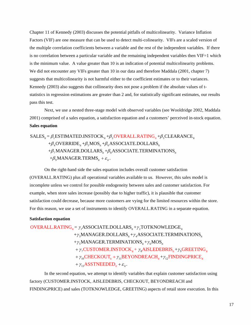
Sales equation

it 1 it 2 3 it

4 it 5 it 6 it

7 it 8

i

it

9

tSALES = ESTIMATED.INSTOCK + + CLEARANCE + OVERRIDE + MOS + ASSOCIATE.DOLLARS + MANAGER.DOLLARS + ASSOCIATE.TERMINATI

OVE

ONS

RALL.RATIN

+ MANAGER.T R

G

E

β β ββ β ββ ββ itMS .itε+

On the right-hand side the sales equation includes overall customer satisfaction

(OVERALL.RATING) plus all operational variables available to us. However, this sales model is

incomplete unless we control for possible endogeneity between sales and customer satisfaction. For

example, when store sales increase (possibly due to higher traffic), it is plausible that customer

satisfaction could decrease, because more customers are vying for the limited resources within the store.

For this reason, we use a set of instruments to identify OVERALL.RATING in a separate equation.

Satisfaction equation

1 it 2 it

3 it 4

t

it

5

i = ASSOCIATE.DOLLARS + TOTKNOWLEDGE + MANAGER.DOLLARS + ASSOCIATE.TERMINATIONS +

OV

MA

ERALL.RA

NAGER.TE

TING

RMINATION

γ γγ γγ it 6 it

7 8 9

10 11 1

it

2

it i

13

t

it it it

it

CUSTOMER.INSTOCK + AISLEDEBRIS GREETINGCHECKOUT BEYONDREACH FIN

S + MOS

DINGPRICEASSTNE

++

EDE .D it

γγ γ γγ γ γγ ε

++

+ +

+

In the second equation, we attempt to identify variables that explain customer satisfaction using

factory (CUSTOMER.INSTOCK, AISLEDEBRIS, CHECKOUT, BEYONDREACH and

FINDINGPRICE) and sales (TOTKNOWLEDGE, GREETING) aspects of retail store execution. In this

18

equation the variables ASSOCIATE.DOLLARS and MANAGER.DOLLARS control for resource

availability within the store to perform both factory and sales functions. All independent variables in this

model act as instruments for OVERALL.RATING in the sales equation. However, just as SALES and

OVERALL.RATING could be codetermined in the sales equation, OVERALL.RATING and

CUSTOMER.INSTOCK can be codetermined in the satisfaction equation. For example, more satisfied

customers would, on average, buy more thus depleting inventory and decreasing in-stock availability for

other customers. This observation requires resolving possible endogeneity using a third equation.

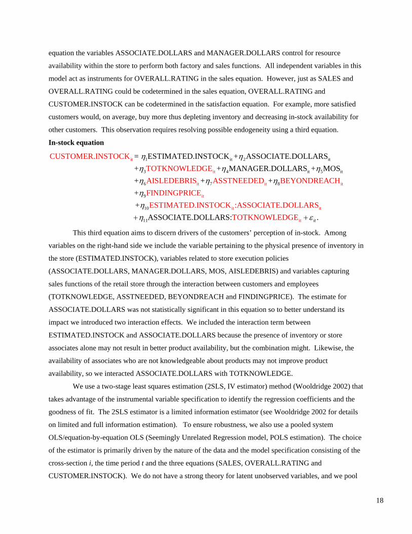
In-stock equation

it

i

1 it 2 it

3 it 4 it 5 t

6

= ESTIMATED.INSTOCK + ASSOCIATE.DOLLARS CUST

+ + MANAGER.DOLLARS + MOS

OMER.INS

TOCKTOTKNO

W

+LEDGE

AISLEDEBR

η ηη η ηη it it it

it

it it

7 8

9

10

11

IS ASSTNEEDED BEYONDREACHFINDINGPRICEESTIMATED.INSTOCK :ASSOCIATE.DOLL

+ + +

+ ASSOCIATE.DOLL

ARSTOTKARS:

η ηηηη+ itNOWLEDGE .itε+

This third equation aims to discern drivers of the customers’ perception of in-stock. Among

variables on the right-hand side we include the variable pertaining to the physical presence of inventory in

the store (ESTIMATED.INSTOCK), variables related to store execution policies

(ASSOCIATE.DOLLARS, MANAGER.DOLLARS, MOS, AISLEDEBRIS) and variables capturing

sales functions of the retail store through the interaction between customers and employees

(TOTKNOWLEDGE, ASSTNEEDED, BEYONDREACH and FINDINGPRICE). The estimate for

ASSOCIATE.DOLLARS was not statistically significant in this equation so to better understand its

impact we introduced two interaction effects. We included the interaction term between

ESTIMATED.INSTOCK and ASSOCIATE.DOLLARS because the presence of inventory or store

associates alone may not result in better product availability, but the combination might. Likewise, the

availability of associates who are not knowledgeable about products may not improve product

availability, so we interacted ASSOCIATE.DOLLARS with TOTKNOWLEDGE.

We use a two-stage least squares estimation (2SLS, IV estimator) method (Wooldridge 2002) that

takes advantage of the instrumental variable specification to identify the regression coefficients and the

goodness of fit. The 2SLS estimator is a limited information estimator (see Wooldridge 2002 for details

on limited and full information estimation). To ensure robustness, we also use a pooled system

OLS/equation-by-equation OLS (Seemingly Unrelated Regression model, POLS estimation). The choice

of the estimator is primarily driven by the nature of the data and the model specification consisting of the

cross-section i, the time period t and the three equations (SALES, OVERALL.RATING and

CUSTOMER.INSTOCK). We do not have a strong theory for latent unobserved variables, and we pool

19

data across stores. The variance-covariance matrix of the residuals and regressors is assumed to be

independent of the cross-section by virtue of the normalization process. In lieu of the standardization

process, one would have to use a FGLS (Feasible Generalized Least Squares) estimator to account for

cross-sectional heterogeneity. Furthermore, to manage the longitudinal component, we approximate

short-run dynamic behavior using forward-looking and AR(k) transformations, thus eliminating the need

to use a dynamic estimation mechanism. That leaves us with the choice of estimating SALES,

OVERALL.RATING and CUSTOMER.INSTOCK either independently or jointly. We perform and

compare both of these estimations. See Wooldridge (2002) for an extensive and detailed exposition of

these estimation techniques.

6. Results and Discussion

The results of both 2SLS and POLS estimations are summarized in Tables 4a-4c. The change in

results from a simple POLS estimation to the 2SLS estimation sheds light on the role of instrumental

variables and is discussed below. The majority of this section discusses the results of the 2SLS estimator,

since it incorporates more information on the simultaneous equations than the POLS estimator. In all

three equations, the F-test and the p-value (<.001) support the null hypothesis of simultaneous and linear

sales, satisfaction and product availability regression models.

Sales equation

The POLS estimator reports that R2=74.6%. ESTIMATED.INSTOCK, ASSOCIATE.DOLLARS,

OVERALL.RATING, MANAGER.DOLLARS and CLEARANCE are statistically significant in the

2SLS regression (p<.01). Judging by the relative magnitude of coefficients, ESTIMATED.INSTOCK

(.176), ASSOCIATE.DOLLARS (.483) and OVERALL.RATING (.202) have the strongest impact on

sales. While other studies have also demonstrated that customer satisfaction (Sulek et al. 1995, Anderson

et al. 2004) and inventory availability (DeHoratius and Raman 2005) positively affect sales, the presence

of associate payroll among impactful variables is new. We argue that store associates are instrumental in

fulfilling both factory and service functions within the store. The reason is that store associates perform a

variety of factory tasks, which include moving inventory from the back room to the shelf, conducting

inventory audits, guarding against theft, updating price stickers, checking adherence to the planogram,

etc. Moreover, store associates perform sales office tasks which involve all facets of customer-employee

contact, such as explaining the location of the products within the store, helping customers to make brand

decisions and manage their shopping baskets, etc. It is also reassuring to see that satisfied customers do

buy more. Interestingly, the amount of merchandise sold on clearance (CLEARANCE, β=.043) has a

much smaller impact on sales. Managerial payroll (MANAGER.DOLLARS, β=.04) has a positive and

statistically significant impact on sales, but it is rather limited compared to the top three variables.

20

Satisfaction equation

TOTKNOWLEDGE, CUSTOMER.INSTOCK, ASSOCIATE.DOLLARS, GREETING,

CHECKOUT, FINDINGPRICE and MOS are statistically significant in the 2SLS regression (p<.01).

The POLS estimator reports that R2=97.1%, indicating excellent goodness of fit. Comparison of absolute

values of the regression coefficients in the 2SLS regression indicates that employee knowledge

(TOTKNOWLEDGE, γ=.571) and customer perception of product availability (CUSTOMER.INSTOCK,

γ=.399) have by far the strongest impact on the OVERALL.RATING. Thus, customer satisfaction is

strongly influenced by both sales (TOTKNOWLEDGE) and factory (CUSTOMER.INSTOCK) functions.

The overwhelming importance of TOTKNOWLDGE suggests that customers greatly value the role of

employees as experts helping them to make decisions on prices, brands and product features. Payroll

(ASSOCIATE.DOLLARS, γ=.018) impacts customer satisfaction less, but its role should not be

underestimated, because the role of employees in factory and sales functions has already been partially

captured by the CUSTOMER.INSTOCK and TOTKNOWLEDGE variables, respectively. As we would

expect, checkout efficiency (CHECKOUT, γ=.064) is positively associated with customer satisfaction,

whereas an inability to find the price (FINDINGPRICE, γ=-.018) and inventory record inaccuracy (MOS,

γ=-.016) are negatively associated with customer satisfaction, results that we intuitively expect. It also

appears that an employee greeting (GREETING, γ=.032) helps to improve customer satisfaction.

In-stock equation

ESTIMATED.INSTOCK, TOTKNOWLEDGE, MOS, MANAGER.DOLLARS,

FINDINGPRICE, ASSTNEEDED and two interaction terms are statistically significant in the 2SLS

estimation (p<.01). The POLS estimator reports that R2=71.34%. The relative magnitude of regression

coefficients indicates that physical inventory availability (ESTIMATED.INSTOCK, η=.218) and

employee knowledge (TOTKNOWLEDGE, η=.597) are the most significant drivers of customers’

perception of product availability. Once again, we see that a combination of the sales function and the

factory function facilitates product availability. However, it is very surprising that the impact of

employee knowledge is almost three times as high as the impact of in-stock. We should note that payroll

(ASSOCIATE.DOLLARS) itself is not significant but two interaction terms involving payroll are

significant (ESTIMATED.INSTOCK:ASSOCIATE.DOLLARS, η=-.056, ASSOCIATE.DOLLARS

:TOTKNOWLEDGE, η=.041). The negative coefficient on ESTIMATED.INSTOCK:ASSOCIATE.

DOLLARS suggests that inventory and employees are substitutes rather than complements. However, the

interaction of payroll and service components (ASSOCIATE. DOLLARS:TOTKNOWLEDGE) has a

positive impact on CUSTOMER.INSTOCK. Thus, knowledgeable employees are instrumental in

facilitating product availability. Additionally, MANAGER.DOLLARS (η=.032) and FINDINGPRICE

21

(η=.031) have small but positive impact on customers’ perception of product availability. The fact that

the customer needed employee assistance and did not find it (ASSTNEEDED, η=-.021) negatively

impacts the perception of product availability, thus again pointing toward the crucial role of employees.

Surprisingly, the proxy for the misplaced inventory (MOS, η=.044) has a positive relationship with

product availability. We propose that MOS captures only the “positive” side of misplaced inventory (i.e.,

customers do find the product even though it is misplaced) and hence translates into higher product

availability.

We note that employee and management turnover is not significant in any of our estimates. We

believe that the reason for this finding might be that our measure of turnover includes voluntary as well as

involuntary terminations, making it hard to distinguish between the positive and negative impacts of

turnover. Likewise, AISLEDEBRIS and BEYONDREACH were never statistically significant,

suggesting that obstructions that prevent customers from reaching products do not seem to play a big role

in either customer satisfaction or the perception of product availability for this particular retailer.

Endogeneity and simultaneous estimation

The POLS estimator conducts equation-by-equation estimation and ignores the simultaneity of

the three equations, whereas the 2SLS estimator incorporates some information about the simultaneity in

the estimation process (see Maddala 2001 for a detailed exposition of limited information estimators). In

our two estimations, coefficients of the regressors differ in both the sales and satisfaction equations.

Notably, in the satisfaction equation, the coefficient of CUSTOMER.INSTOCK is higher and the

coefficient for TOTKNOWLEDGE is lower in the 2SLS estimator, because the 2SLS estimator

incorporates information about the instruments for CUSTOMER.INSTOCK. Possible reason is that

OVERALL.RATING has a negative impact on CUSTOMER.INSTOCK because satisfied customers

deplete inventory faster. Moreover, TOTKNOWLEDGE has a very strong direct effect on

CUSTOMER.INSTOCK (as is evident from the third equation) in addition to affecting

OVERALL.RATING directly. MANAGER.DOLLARS becomes insignificant in the 2SLS estimation,

because it is very significant in the CUSTOMER.INSTOCK equation.

In the sales equation, the coefficient of ESTIMATED.INSTOCK decreases and the coefficient of

the OVERALL.RATING increases in the 2SLS estimation relative to POLS estimation. The 2SLS

estimate of the OVERALL.RATING coefficient .202 (>.138) is the gross impact of OVERALL.RATING

on SALES, and the POLS estimate (.138) is an approximation of the net impact of OVERALL.RATING

on SALES after accounting for the negative feedback effect of SALES on OVERALL.RATING.

Moreover, whereas the 2SLS estimator shows the direct impact of ESTIMATED.INSTOCK on SALES

(.176), the POLS estimator overestimates this coefficient (.223) by including the indirect effect

(ESTIMATED.INSTOCK CUST.INSTOCK OVERALL.RATING SALES) in its estimation.

22

We summarize the results of 2SLS estimates in Figure 1, where we show only the explanatory variables

that exert the greatest impact while keeping the diagram as simple as possible.

7. Managerial Implications

The research effort reported here is part of a larger project that includes Nicole DeHoratius as a

member of the research team and three retailers in addition to the one discussed here. The overall project

seeks to understand broadly what store operating policies lead to effective execution. As part of this

broader project, we interviewed several dozen individuals, including executives at the four participating

retailers, together with executives at other retailers and consultants and academics with expertise in

retailing. Figure 2 depicts a conceptual model of store operations that is consistent both with these

interviews and with the results of our data analysis. Each day a given customer traffic arrives at a store

representing potential demand. A fraction of this potential demand converts to actual sales depending on

how well the store executes. Potential demand may fail to convert to actual sales if the store fails on any

of four key execution elements: 1) the product the customer wants to buy isn’t in the store because of a

stock-out 2) the customer needs help and can’t find a store associate 3) they find an associate but the

associate is not helpful or 4) the checkout line is too long. We do not intend this as a universal model that

captures everything important in all stores for all retailers, but rather a parsimonious model that, given

what we saw in our data analysis, appears to fit store operations of the retailer we studied. As one

example of a factor omitted from this model that might be important to other retailers, several experts told

us managing adjacencies of products to drive add-on purchases is important in some contexts.

If customers find what they came for and make purchase successfully, they leave the store

satisfied, and are likely to return. Otherwise, they will abandon this retailer for a competitor with some

probability. Thus, in this model, sales during the current visit increases satisfaction, which in turn leads to

future visits and sales. This model is also consistent with many findings in the literature. Much of

classical inventory management literature (see, e.g., Cachon and Terwiesch 2005) is predicated on the

assumption that in-stock is a driver of sales. The role of the store associate in guiding customer purchase

decisions is documented in the marketing literature (see Sulek et al. 1995, Iacobucci et al. 1994, 1995) as

well as in studies of retail banking (Frei and Harker 1999). Iacobucci et al. (1994, 1995) document that

satisfaction is an outcome of good service. Furthermore, DeHoratius and Raman (2003) document the

role of store associates in getting products on the shelves and aiding customers in their search for the

product

Our analysis provides sufficient data to assess the impact on sales of changes in store associate

staffing. Note that given the data transformation to control for store heterogeneity, the coefficient of .483

on store associate payroll in the sales equation implies that increasing associate payroll at store i by

23

σASSOCIATE.DOLLARS i increases sales by σSALES i. We can thus calculate the increase in monthly store sales

from a $1 increase in monthly store payroll at store i as .483σSALES i/σASSOCIATE.DOLLARS i. We found these

lift factors varied considerably across stores, ranging from a low of $3.94 to a high of $28.01.

One obvious question is what causes the variation in payroll elasticity across stores. To

understand this, first note that intuitively one would expect a diminishing return on each additional store

associate added (with an arbitrarily large increase in staffing, associates would eventually outnumber

customers and additional staff would be expected to have little impact) and hence sales as a function of

payroll should be a concave, non-decreasing function. Figure 3 shows sales vs. payroll for a

representative store over time and we do indeed see this concave shape exhibited. The sales lifts we have

computed for payroll increases are essentially the derivative of this curve at the current staffing level for

each store. Hence, we hypothesize that those stores with high (low) lifts are currently staffed at a low

(high) level relative to sale and hence are on the steep (flat) part of this curve. We examined the data and

found that those stores with high lift values also had a high ratio of sales to associate payroll relative to

stores with low lift values.

This retailer earns gross margins of about 40%, so even for the lowest sales lift of 3.94,

incremental profit of .4*3.94 = $1.58 exceeds the additional $1 expense. It thus appeared that this retailer

would benefit from an increased staffing level at all stores. However, a significant increase in a major

expense such as payroll is controversial and may have other ramifications. On the other hand, the

allocation of staffing across stores via the planned payroll budget is something that is evaluated every

month. Hence, we explored the use of our analysis to guide a better allocation of associate payroll across

stores. We sorted the sales lift of stores open for at least one year in our data and found that the 236 stores

with the lowest lifts had total monthly payroll of $5,375,052 vs. a nearly equal value of $5,384,640 for the

remaining 201 stores with highest lift. Increasing monthly payroll by 25% (an amount we judged to be

within the range of linearity on the concave sales vs payroll curve) for the 201 stores with highest lift and

lowering payroll by 25.05% for remaining stores would leave total chain payroll unchanged and increase

sales by 2.6%. Public retailers routinely report sales increases in stores open at least one year, called

comp sales. Generally comp sales range from negative to the low single digits, so a 2.6% sales increase is

significant. Retailers also use a large number of part time employees and by varying the hours of these

employees it’s possible to vary payroll nearly continuously.

We also computed the increase in sales at each store from a 1% increase in in-stock. These factors

had a 92% correlation with store sales and varied nearly linearly with store sales, consistent with a model

that stock-outs simply reduce store sales in proportion to the level of stock-outs. Lift factors average 20%

of sales, suggesting that when a customer encounters a stock-out, they substitute with another product

80% of the time. This is the only study we are aware of to present evidence of customer stock-out rates in

24

a large scale situation. Note that the ‘factor of production’ analogous to store payroll is not in-stock, but

the inventory which drives in-stock. While we found that sales varies linearly with in-stock, in-stock as a

function of inventory is a concave non-increasing function, and hence sales vs. inventory has the same

form as sales vs. associate payroll.

Clearly, with both inventory and payroll, there is an optimal level at which marginal return equals

marginal cost. It is difficult to find this optimal level directly for payroll because our analysis provides

only the derivative of a non linear curve. However, we were able to suggest an improving adjustment to

payroll, and this process repeated over time would tend to an optimal point. If one assumes the 80%

substitution rate inferred by our analysis applies across all products, it would be possible to conduct SKU

level analysis using known theory to find inventory levels that minimize the cost of lost margin due to

stockouts and carrying costs.

Clearly, results of our analysis should be used with caution because they are limited to the

particular retailer that we studied. For example, the impact that employee knowledge has on customers’

perception of product availability will probably differ between grocery and electronics retailers. By

extension, the relative importance of the sales and the factory functions will differ from retailer to retailer

as well. However, we do believe that the methodology we propose is quite general and can be applied by

other retailers that conduct surveys of customer satisfaction and track operational metrics within the store.

Although we focused on explaining month-to-month variations in sales, satisfaction and product

availability, we might pose a different question: What explains the average and standard deviation of sales

at different stores (the cross-sectional study)? We suspect that the main factors in such a study will be

customer demographics, the presence of competition, physical store characteristics, advertising, and the

characteristics of store employees and managers, among others. The only previous study that focuses on

explaining cross-sectional variations in retail store performance, at least that we are aware of, is Hise et al.

(1983), who find that the number of employees, inventory, store size, fixed assets and employee tenure

with the company are associated with sales, to a statistically significant degree.

References

Anderson, S. W., L. S. Baggett and S. K. Widener. 2006. The impact of service operations failures on

customer satisfaction: the role of attributions of blame. Working paper, Rice University.

Anderson, E.W., C. Fornell and S. K. Mazvancheryl. 2004. Customer satisfaction and shareholder value.

Journal of Marketing, 68(4), 172-185.

Babakus, E., C. C. Bienstock, and J. R. Van Scotter. 2004. Linking perceived quality and customer

25

satisfaction to store traffic and revenue growth. Decision Sciences, 35(4), 713-737.

Cachon, G. and C. Terwiesch. 2005. Matching Supply with Demand: An Introduction to Operations

Management. 1st ed., McGraw-Hill.

Corsten, D. and T. Gruen. 2003. Seeking on-shelf availability—an examination of the extent, the causes

and the efforts to address retail out-of-stocks. International Journal of Retail and Distribution

Management, 31(12), 605-716.

DeHoratius, N. and A. Raman. 2003. Building on foundations of sand? ECR Journal, 3(1), 62-63.

DeHoratius, N. and A. Raman. 2006. Store management incentive design and retail performance: an

exploratory investigation. Forthcoming in Manufacturing & Services Operations Management.

Denove, C. and J. D. Power IV. 2006. Satisfaction: how every great company listens to the voice of the

customer. 1st ed., Penguin Books, Ltd.

Erdem, T. and M. Keane. 1996. Decision-making under uncertainty: capturing dynamic brand choice

processes in turbulent consumer markets. Marketing Science, 15(1), 1-20.

Fisher, M. L. 2004. To me it’s a factory, to you it’s a store. ECR Journal, 4(2), 9-18.

Fisher M. L., C. Ittner. 1999. The impact of product variety on automobile assembly operations: empirical

evidence and simulation analysis. Management Science, 45, 771-786.

Fisher, M. L. and J. Krishnan. 2005. Gotta Hava Wawa. Case study, The Wharton School, University of

Pennsylvania.

Fisher, M. L., A. Raman and A. McClelland. 2000. Rocket-science retailing is almost here: are you

ready? Harvard Business Review, 78(4), 115-124.

Frei, F. X. and P. T. Harker. 1999. Measuring the efficiency of service delivery processes: an application

to retail banking. Journal of Service Research, 1(4), 300-312.

Frei, F. X., R. Kalakota, A. J. Leone and L. M. Marx. 1999. Process variation as determinant of bank

performance: evidence from the retail banking study. Management Science, 45(9), 1210-1220.

Hise, R. T., J. P. Kelly, M. Gable and J. B. McDonald. 1983. Factors affecting the performance of

individual chain store units: an empirical analysis. Journal of Retailing, 59(2), 22-39.

26

Iacobucci, D., K. Grayson and A. Ostrom. 1994. The calculus of service quality and customer

satisfaction: theoretical and empirical differentiation and integration, in T.A. Swartz, D.E. Bowen,

and S.W. Brown, eds., Advances in Services Marketing and Management: Research and Practice,

Vol. 3, Greenwich, CT: JAI Press, 1-67.

Iacobucci, D., A. Ostrom and K. Grayson. 1995. Distinguishing service quality and customer satisfaction:

the voice of the consumer. Journal of Consumer Psychology, 4, 277-303.

Ittner, C. D., and D. F. Larcker. 1998. Are non-financial measures leading indicators of financial

performance? An analysis of customer satisfaction. Journal of Accounting Research, 36, 1-46.

Kennedy, P. 2003. A Guide to Econometrics. 5th ed., The MIT Press.

Lapre, M. A. and N. Tsikriktsis. 2006. Organizational learning curves for customer dissatisfaction:

heterogeneity across airlines. Management Science, 52, 352-366.

MacDuffie, J. P., K. Sethuraman and M. L. Fisher. 1996. Product variety and manufacturing performance:

evidence from the international automotive assembly plant study. Management Science, 42(3), 350-

369.

Maddala, G. S., 2001. Introduction to Econometrics. 3rd ed., John Wiley & Sons

Mittal, V., E. W. Anderson, A. Sayrak and P. Tadikamalla. 2005. Dual emphasis and the long-term

financial impact of customer satisfaction. Marketing Science, 24(4), 544-555.

Morgan, N.A. and L.L. Rego. 2006. The value of different customer satisfaction and loyalty metrics in

predicting business performance. Marketing Science, 25(5), 426-439.

Pindyck, R. S. and D. L. Rubinfeld. 1997. Econometric Models and Economic Forecasts. 4th ed.,

McGraw-Hill/Irwin.

Raman, A., N. DeHoratius and Z. Ton. 2001a. The Achilles heel of supply chain management. Harvard

Business Review, May, 136-152.

Raman, A., N. DeHoratius and Z. Ton. 2001b. Execution: the missing link in retail operations. California

Management Review, 43(3), 136-142.

Ren, J. and X. Wang. 2006a. Process consistency and service quality in US hospitals: an empirical

27

investigation. Working Paper, Boston University.

Ren, J. and X. Wang. 2006b. Volume and variability: an empirical investigation of service quality in US

hospitals. Working Paper, Boston University.

Salmon, W. J. 1989. Retailing in the age of execution. Journal of Retailing, 65(3), 368-378.

Spector, R. and D. McCarthy. 1996. The Nordstrom way: the inside story of America’s #1 customer

service company. Reprint ed., John Wiley & Sons.

Sulek, J. M., M. R. Lind and A. S. Marucheck. 1995. The impact of customer service intervention and

facility design on firm performance. Management Science, 41(11), 1763-1773.

Ton, Z. and R. S. Huckman. 2005. Managing the impact of employee turnover on performance: the role

of process conformance. Working paper, Harvard University.

Ton, Z. and A. Raman. 2004. The effect of product variety and inventory levels on retail store operations:

a longitudinal study. Working paper, Harvard University.

Tsikriktsis, N. 2006. The effect of operational performance and focus on profitability: a longitudinal study

of the U.S. airline industry. Forthcoming, Manufacturing & Service Operations Management.

Tucker, A. 2004. The impact of operational failures on hospital nurses and their patients. Journal of

Operations Management, 22(2), 151-169.

Tucker, A., and A. Edmondson. 2003. Why hospitals don't learn from failures: organizational and

psychological dynamics that inhibit system change. California Management Review, 45(2), 55-72.

van Donselaar, K. H., V. Gaur, T. van Woensel, R. A. C. M. Broekmeulen and J. C. Fransoo. 2006. An

empirical study of ordering behavior of retail stores. Working paper, Eindhoven University of

Technology.

Womack, J. P., D. T. Jones and D. Roos. 1991. The machine that changed the world: the story of lean

production. Reprint ed., Harper Perennial.

Wooldridge, J. M. 2002. Econometric analysis of cross section and panel data. 1st ed., The MIT Press.

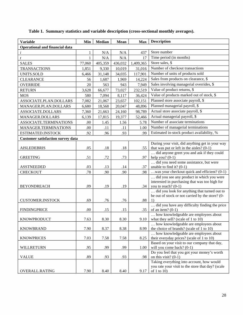
28

Table 1. Summary statistics and variable description (cross-sectional monthly averages).

Variable Min Median Mean Max Description Operational and financial data i 1 N/A N/A 437 Store number t 1 N/A N/A 17 Time period (in months) SALES 77,060 405,359 436,032 1,409,365 Store sales, $ TRANSACTIONS 1,851 9,330 10,019 31,016 Number of checkout transactions UNITS.SOLD 6,466 31,148 34,035 117,901 Number of units of products sold CLEARANCE 56 1,687 1,969 14,224 Sales from products on clearance, $ OVERRIDE 20 563 943 7,949 Sales involving managerial overrides, $ RETURN 3,628 66,677 73,027 232,519 Value of product returns, $ MOS 580 7,094 8,117 36,424 Value of products marked out of stock, $ ASSOCIATE.PLAN.DOLLARS 7,082 21,067 23,657 102,151 Planned store associate payroll, $ MANAGER.PLAN.DOLLARS 6,680 18,568 20,047 48,896 Planned managerial payroll, $ ASSOCIATE.DOLLARS 7,360 21,663 24,160 98,789 Actual store associate payroll, $ MANAGER.DOLLARS 6,139 17,815 19,377 52,466 Actual managerial payroll, $ ASSOCIATE.TERMINATIONS .00 1.45 1.56 5.78 Number of associate terminations MANAGER.TERMINATIONS .00 .11 .11 1.00 Number of managerial terminations ESTIMATED.INSTOCK .92 .96 .93 .99 Estimated in-stock product availability, % Customer satisfaction survey data

AISLEDEBRIS .05 .18 .18 .55 During your visit, did anything get in your way that was put or left in the aisles? (0-1)

GREETING .51 .72 .73 .97 … did anyone greet you and ask if they could help you? (0-1)

ASSTNEEDED .03 .13 .14 .37 … did you need some assistance, but were unable to find it? (0-1)

CHECKOUT .78 .90 .90 .98 …was your checkout quick and efficient? (0-1)

BEYONDREACH .09 .19 .19 .34

… did you see any product in which you were interested in purchasing that was too high for you to reach? (0-1)

CUSTOMER.INSTOCK .69 .76 .76 .88

… did you look for anything that turned out to be out of stock or not carried by the store? (0-1)

FINDINGPRICE .00 .15 .15 .35 … did you have any difficulty finding the price of an item? (0-1)

KNOWPRODUCT 7.63 8.30 8.30 9.10 … how knowledgeable are employees about what they sell? (scale of 1 to 10)

KNOWBRAND 7.90 8.37 8.38 8.99 … how knowledgeable are employees about the choice of brands? (scale of 1 to 10)

KNOWPRICES 7.03 7.58 7.58 8.25 … how knowledgeable are employees about their everyday prices? (scale of 1 to 10)

WILLRETURN .95 .99 .99 1.00 Based on your visit to our company that day, will you come back? (0-1)

VALUE .89 .93 .93 .98 Do you feel that you got your money’s worth on this visit? (0-1)

OVERALL.RATING 7.90 8.40 8.40 9.17

Taking everything into account, how would you rate your visit to the store that day? (scale of 1 to 10)

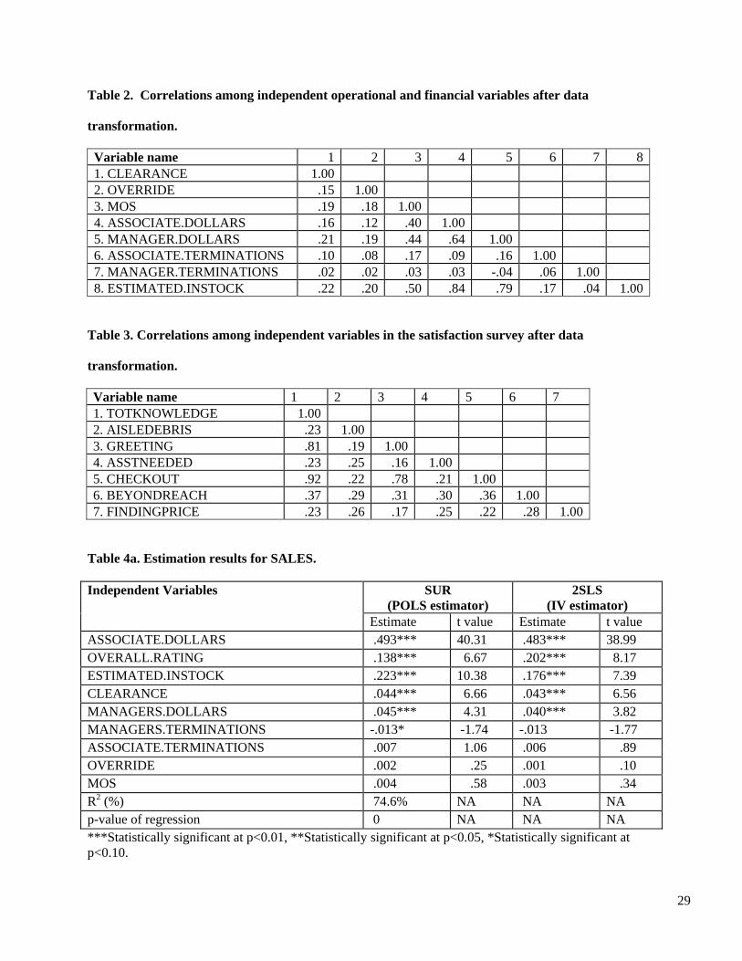
29

Table 2. Correlations among independent operational and financial variables after data

transformation.

Variable name 1 2 3 4 5 6 7 81. CLEARANCE 1.00 2. OVERRIDE .15 1.00 3. MOS .19 .18 1.00 4. ASSOCIATE.DOLLARS .16 .12 .40 1.00 5. MANAGER.DOLLARS .21 .19 .44 .64 1.00 6. ASSOCIATE.TERMINATIONS .10 .08 .17 .09 .16 1.00 7. MANAGER.TERMINATIONS .02 .02 .03 .03 -.04 .06 1.00 8. ESTIMATED.INSTOCK .22 .20 .50 .84 .79 .17 .04 1.00

Table 3. Correlations among independent variables in the satisfaction survey after data

transformation.

Variable name 1 2 3 4 5 6 7 1. TOTKNOWLEDGE 1.00 2. AISLEDEBRIS .23 1.00 3. GREETING .81 .19 1.00 4. ASSTNEEDED .23 .25 .16 1.00 5. CHECKOUT .92 .22 .78 .21 1.00 6. BEYONDREACH .37 .29 .31 .30 .36 1.00 7. FINDINGPRICE .23 .26 .17 .25 .22 .28 1.00

Table 4a. Estimation results for SALES.

SUR (POLS estimator)

2SLS (IV estimator)

Independent Variables

Estimate t value Estimate t value ASSOCIATE.DOLLARS .493*** 40.31 .483*** 38.99 OVERALL.RATING .138*** 6.67 .202*** 8.17 ESTIMATED.INSTOCK .223*** 10.38 .176*** 7.39 CLEARANCE .044*** 6.66 .043*** 6.56 MANAGERS.DOLLARS .045*** 4.31 .040*** 3.82 MANAGERS.TERMINATIONS -.013* -1.74 -.013 -1.77 ASSOCIATE.TERMINATIONS .007 1.06 .006 .89 OVERRIDE .002 .25 .001 .10 MOS .004 .58 .003 .34 R2 (%) 74.6% NA NA NA p-value of regression 0 NA NA NA ***Statistically significant at p<0.01, **Statistically significant at p<0.05, *Statistically significant at p<0.10.

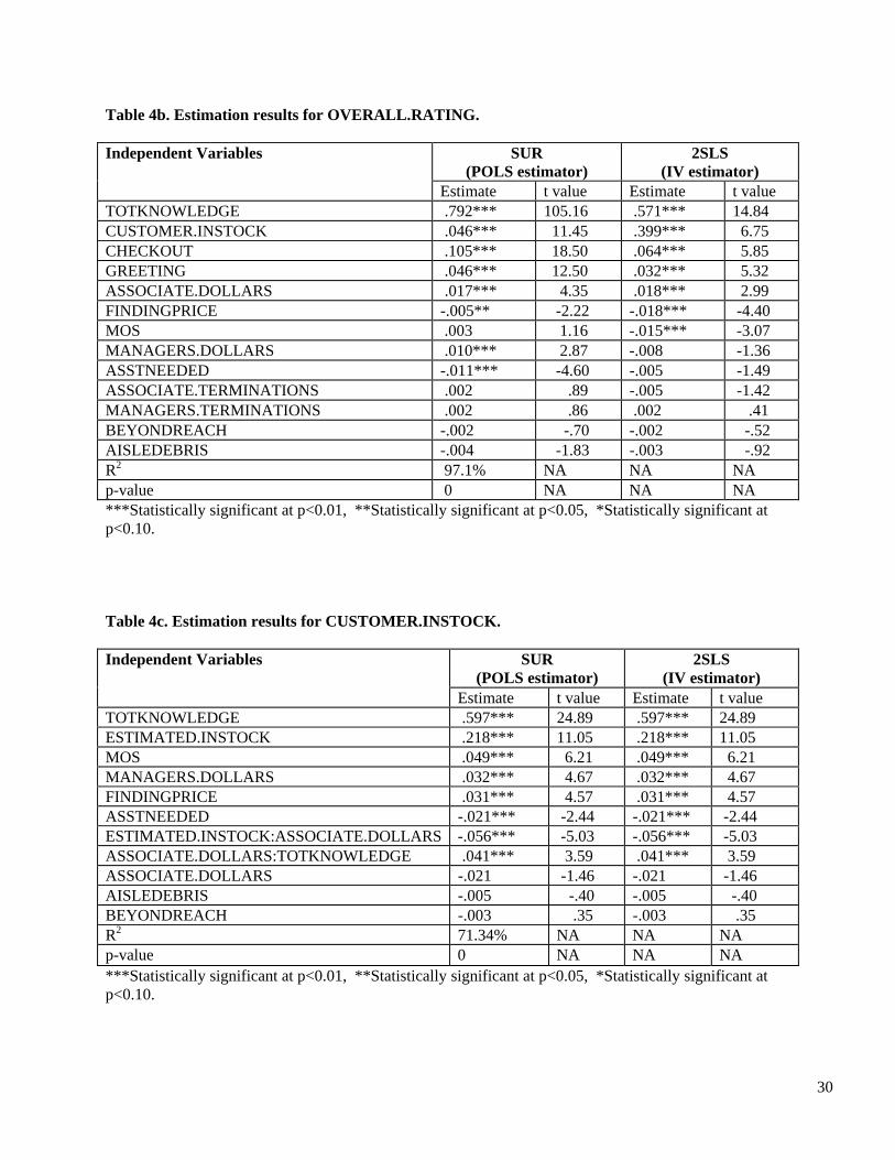
30

Table 4b. Estimation results for OVERALL.RATING.

SUR (POLS estimator)

2SLS (IV estimator)

Independent Variables

Estimate t value Estimate t value TOTKNOWLEDGE .792*** 105.16 .571*** 14.84 CUSTOMER.INSTOCK .046*** 11.45 .399*** 6.75 CHECKOUT .105*** 18.50 .064*** 5.85 GREETING .046*** 12.50 .032*** 5.32 ASSOCIATE.DOLLARS .017*** 4.35 .018*** 2.99 FINDINGPRICE -.005** -2.22 -.018*** -4.40 MOS .003 1.16 -.015*** -3.07 MANAGERS.DOLLARS .010*** 2.87 -.008 -1.36 ASSTNEEDED -.011*** -4.60 -.005 -1.49 ASSOCIATE.TERMINATIONS .002 .89 -.005 -1.42 MANAGERS.TERMINATIONS .002 .86 .002 .41 BEYONDREACH -.002 -.70 -.002 -.52 AISLEDEBRIS -.004 -1.83 -.003 -.92 R2 97.1% NA NA NA p-value 0 NA NA NA ***Statistically significant at p<0.01, **Statistically significant at p<0.05, *Statistically significant at p<0.10.

Table 4c. Estimation results for CUSTOMER.INSTOCK.

SUR (POLS estimator)

2SLS (IV estimator)

Independent Variables

Estimate t value Estimate t value TOTKNOWLEDGE .597*** 24.89 .597*** 24.89 ESTIMATED.INSTOCK .218*** 11.05 .218*** 11.05 MOS .049*** 6.21 .049*** 6.21 MANAGERS.DOLLARS .032*** 4.67 .032*** 4.67 FINDINGPRICE .031*** 4.57 .031*** 4.57 ASSTNEEDED -.021*** -2.44 -.021*** -2.44 ESTIMATED.INSTOCK:ASSOCIATE.DOLLARS -.056*** -5.03 -.056*** -5.03 ASSOCIATE.DOLLARS:TOTKNOWLEDGE .041*** 3.59 .041*** 3.59 ASSOCIATE.DOLLARS -.021 -1.46 -.021 -1.46 AISLEDEBRIS -.005 -.40 -.005 -.40 BEYONDREACH -.003 .35 -.003 .35 R2 71.34% NA NA NA p-value 0 NA NA NA ***Statistically significant at p<0.01, **Statistically significant at p<0.05, *Statistically significant at p<0.10.

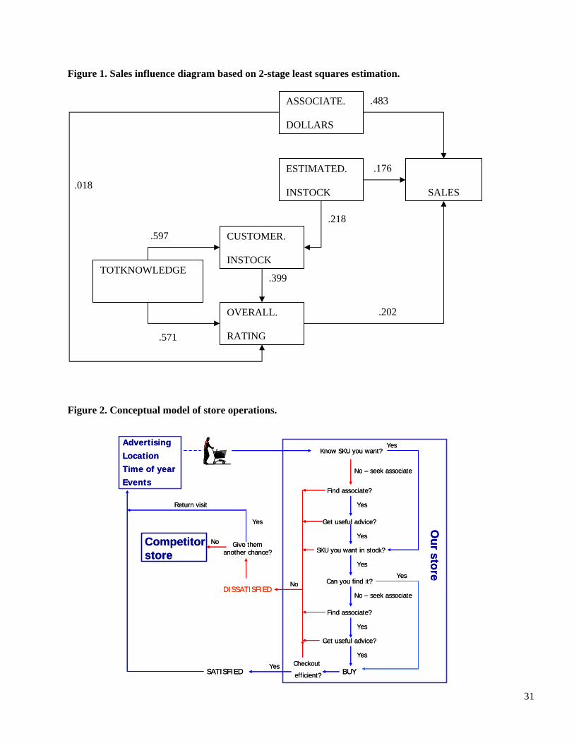
31

Figure 1. Sales influence diagram based on 2-stage least squares estimation.

Figure 2. Conceptual model of store operations.

.018

.218

.399

.202

.571

.597

.176

.483 ASSOCIATE.

DOLLARS

ESTIMATED.

INSTOCK

CUSTOMER.

INSTOCK

OVERALL.

RATING

TOTKNOWLEDGE

SALES

Know SKU you want?

Find associate?

Get useful advice?

SKU you want in stock?

Can you find it?

Find associate?

Get useful advice?

BUY

Yes

No – seek associate

Yes

Yes

Yes

Yes

Yes

Yes

Return visit

SATISFIED

AdvertisingLocationTime of yearEvents

DISSATISFIED

Give them another chance?

Competitor store

Our store

Yes

No

No – seek associate

No

Checkout

efficient?Yes

Know SKU you want?

Find associate?

Get useful advice?

SKU you want in stock?

Can you find it?

Find associate?

Get useful advice?

BUY

Yes

No – seek associate

Yes

Yes

Yes

Yes

Yes

Yes

Return visit

SATISFIED

AdvertisingLocationTime of yearEvents

DISSATISFIED

Give them another chance?

Competitor store

Our store

Yes

No

No – seek associate

No

Checkout

efficient?Yes

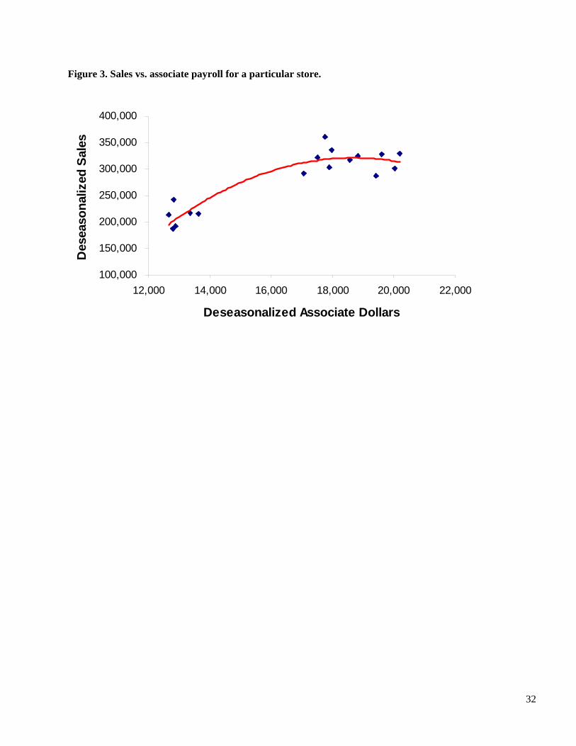
32

Figure 3. Sales vs. associate payroll for a particular store.

100,000

150,000

200,000

250,000

300,000

350,000

400,000

12,000 14,000 16,000 18,000 20,000 22,000

Deseasonalized Associate Dollars

Des

easo

naliz

ed S

ales