Embed Size (px)
Citation preview
University of Arkansas, FayettevilleScholarWorks@UARK
Theses and Dissertations
5-2014
Detailed Inventory Record Inaccuracy AnalysisHayrettin Kaan OkyayUniversity of Arkansas, Fayetteville
Follow this and additional works at: http://scholarworks.uark.edu/etd
Part of the Industrial Engineering Commons, Operational Research Commons, and theOperations and Supply Chain Management Commons
This Dissertation is brought to you for free and open access by ScholarWorks@UARK. It has been accepted for inclusion in Theses and Dissertations byan authorized administrator of ScholarWorks@UARK. For more information, please contact [email protected], [email protected].
Recommended CitationOkyay, Hayrettin Kaan, "Detailed Inventory Record Inaccuracy Analysis" (2014). Theses and Dissertations. 1045.http://scholarworks.uark.edu/etd/1045
Detailed Inventory Record Inaccuracy Analysis
Detailed Inventory Record Inaccuracy Analysis
A dissertation submitted in partial fulfillment of the requirements for the degree of
Doctor of Philosophy in Industrial Engineering
by
Hayrettin Kaan Okyay Koç University
Bachelor of Science in Industrial Engineering, 2008 Koç University
Master of Science in Industrial Enginerring and Operations Management, 2010
May 2014 University of Arkansas
This dissertation is approved for recommendation to the Graduate Council.
______________________________ ______________________________ Dr. Nebil Buyurgan Dr. Shengfan Zhang
Dissertation Co-director Dissertation Co-director
______________________________ ______________________________ Dr. Edward A. Pohl Dr. M. Alp Ertem Committee Member Committee Member
ABSTRACT
This dissertation performs a methodical analysis to understand the
behavior of inventory record inaccuracy (IRI) when it is influenced by
demand, supply and lead time uncertainty in both online and offline retail
environment separately. Additionally, this study identifies the
susceptibility of the inventory systems towards IRI due to conventional
perfect data visibility assumptions. Two different alternatives for such
methods are presented and analyzed; the IRI resistance and the error control
methods. The discussed methods effectively countered various aspects of IRI;
the IRI resistance method performs better on stock-out and lost sales,
whereas error control method keeps lower inventory. Furthermore, this
research also investigates the value of using a secondary source of
information (automated data capturing) along with traditional inventory
record keeping methods to control the effects of IRI. To understand the
combined behavior of the pooled data sources an infinite horizon discounted
Markov decision process (MDP) is generated and optimized. Moreover, the
traditional cost based reward structure is abandoned to put more emphasis on
the effects of IRI. Instead a new measure is developed as inventory
performance by combining four key performance metrics; lost sales, amount of
correction, fill rate and amount of inventory counted. These key metrics are
united under a unitless platform using fuzzy logic and combined through
additive methods. The inventory model is then analyzed to understand the
optimal policy structure, which is proven to be of a control limit type.
TABLE OF CONTENTS
Abstract.................................................................... 3 Table of Contents........................................................... 4 List of Figures............................................................. 6 List of Tables.............................................................. 8 Chapter 1 Introduction...................................................... 1 1.1 Background and Motivation ............................................. 1 1.2 Literature review ..................................................... 3 1.2.1 Inventory Record Inaccuracy ....................................... 4 1.2.2 Multi-Objective Inventory Models .................................. 9
1.3 Organization of the Dissertation ..................................... 12 References................................................................. 15 Chapter 2 IRI Analysis in Offline Retailing with Lead Time and Supply Uncertainty................................................................ 18 2.1 Model ................................................................ 20 2.1.1 Error Modeling ................................................... 23 2.1.2 General Inventory Formulation .................................... 25 2.1.3 Numerical Study .................................................. 27
2.2 Evaluation of the Impact of IRI ...................................... 33 2.2.1 Freezing Potential ............................................... 33 2.2.2 IRI Resistance Method ............................................ 37 2.2.3 Error Control and Correction Method .............................. 42 2.2.4 IRI Resistance and Error Control ................................. 46
2.3 Conclusion and Future Work ........................................... 49 References................................................................. 52 Appendix A................................................................. 54 A.I Best Case Error Calculation .......................................... 54 A.II Worst Case Error Calculation ........................................ 58 A.III Worst Case Combined ................................................ 60
Chapter 3 IRI Analysis in Online Retailing with Lead Time and Supply Uncertainty................................................................ 63 3.1 Model ................................................................ 64 3.1.1 Error Modeling ................................................... 67 3.1.2 General Inventory Formulation .................................... 69 3.1.3 Numerical Study .................................................. 75
3.2 Evaluation of the Impact of IRI ...................................... 78 3.2.1 IRI Resistance Method ............................................ 79 3.2.2 Error Control and Correction Method .............................. 83 3.2.3 IRI Resistance and Error Control ................................. 86
3.3 Conclusion and Future Work ........................................... 89 References................................................................. 91 Chapter 4 Comparative Analysis............................................. 93 4.1 Model ................................................................ 94 4.2 Numerical Study: The Offline Retail Setting .......................... 97 4.2.1 IRI Resistance Method ............................................ 98 4.2.2 Error Control and Correction Method ............................. 102
4.3 Numerical Study: The Online Setting ................................. 105 4.3.1 IRI Resistance Method ........................................... 105 4.3.2 Error Control and Correction Method ............................. 108
4.4 Comparison of Retail Environments ................................... 111 4.5 Retail environments ................................................. 112
References................................................................ 114 Chapter 5 Fuzzy Multi-Objective MDP Model for Inventory Record Inaccuracy. 115
5.1 Model ............................................................... 117 5.1.1 State Space: .................................................... 119 5.1.2 Action Space .................................................... 121 5.1.3 Transition Probabilities ........................................ 122 5.1.4 Reward: Inventory Performance ................................... 125 5.1.5 Infinite-Horizon Discounted MDP ................................. 137
5.2 Structural Properties ............................................... 138 5.2.1 Transition Matrix ............................................... 138 5.2.2 Rewards ......................................................... 139 5.2.3 Value Function and Policy ....................................... 143
5.3 Numerical Analysis .................................................. 146 5.3.1 Transition Matrix ............................................... 146 5.3.2 Rewards ......................................................... 151 5.3.3 Value Function and Policy ....................................... 152
5.4 Conclusion and Future Work .......................................... 153 References................................................................ 155 Chapter 6 Conclusion...................................................... 158
LIST OF FIGURES
Figure 2-1: Behavior of the physical stock, inventory stock, and inventory position................................................................... 21 Figure 2-2: The best (left) and the worst (right) case inventory behavior.. 26 Figure 2-3: The relation between records and errors........................ 33 Figure 2-4: Increasing the safety stock.................................... 38 Figure 2-5: IRI Resistance method for the best and the worst cases......... 39 Figure 2-6: IRI Resistance method for the best and the worst cases cont.... 41 Figure 2-7: The error control method for the best (left) and the worst (right) case............................................................... 44 Figure 2-8: The error control method for the best (left) and the worst (right) case cont.......................................................... 45 Figure 2-9: Combined compensation framework................................ 46 Figure 2-10: Combined method results for recorded and actual inventory for the best case.............................................................. 47 Figure 2-11: Combined method results for lost sales and stock-outs for the best case.................................................................. 47 Figure 2-12: Combined method results for error correction and count number for the best case.......................................................... 48 Figure 2-13: Combined method results for sales and error for the best case. 48 Figure A-1: Combined method results for the worst case..................... 61 Figure A-2: Combined method results for the worst case (cont.)............. 62 Figure 3-1: Behavior of the physical stock, the inventory record, and the inventory position......................................................... 65 Figure 3-2: The relation between the records and the errors................ 66 Figure 3-3: The best (left) and the worst (right) case inventory behavior.. 69 Figure 3-4: Increasing safety stock........................................ 80 Figure 3-5: The IRI resistance method for the best (left) and the worst (right) case............................................................... 81 Figure 3-6: The IRI resistance method for the best (left) and the worst (right) case cont.......................................................... 82 Figure 3-7: The error control method for the best (left) and the worst (right) case............................................................... 84 Figure 3-8: The error control method for the best (left) and the worst (right) case cont.......................................................... 85 Figure 3-9: Combined compensation framework................................ 86 Figure 3-10: Combined method results for penalty sales and lost sales for the best case.................................................................. 87 Figure 3-11: Combined method results for correction and count number for the best case.................................................................. 87 Figure 4-1: Profit function for each scenario for the best case with the IRI resistance method......................................................... 101 Figure 4-2: Profit function for each scenario for the worst case with the IRI resistance method......................................................... 101 Figure 4-3: Profit function for each scenario for the best case with the error control method...................................................... 104 Figure 4-4: Profit function for each scenario for the worst case with the error control method...................................................... 105 Figure 4-5: Profit function for each scenario for the best case with the IRI resistance method......................................................... 107 Figure 4-6: Profit function for each scenario for the worst case with the IRI resistance method......................................................... 108
Figure 4-7: Profit function for each scenario for the best case with the error control method...................................................... 110 Figure 4-8: Profit function for each scenario for the worst case with the error control method...................................................... 110 Figure 5-1: State Space................................................... 120 Figure 5-2: Action space.................................................. 122 Figure 5-3: (A) Membership function for Lost sales and (B) membership function with bounds...................................................... 129 Figure 5-4: (A) Membership function for correction and (B) membership function with bounds...................................................... 131 Figure 5-5: (A) Membership function for service level and (B) membership function with bounds...................................................... 133 Figure 5-6: (A) Membership function for counting amount and (B) membership function with bounds...................................................... 135 Figure 5-7: Probability of visibility discrepancy for 4 states for high performance............................................................... 147 Figure 5-8: Probability of visibility discrepancy for 4 states for medium performance............................................................... 148 Figure 5-9: Probability of visibility discrepancy for 4 states for low performance............................................................... 149 Figure 5-10: Transition probability matrix for 4 states for high performance.......................................................................... 149 Figure 5-11: Transition probability matrix for 4 states for medium performance............................................................... 150 Figure 5-12: Transition probability matrix for 4 states for low performance.......................................................................... 150
LIST OF TABLES
Table 1-1: Dissertation organization....................................... 13 Table 2-1: Correlation matrix of 7 different types of errors in the best case........................................................................... 29 Table 2-2: Covariance matrix of 7 different types of errors in the best case........................................................................... 29 Table 2-3: Summary of statistics of the best case.......................... 30 Table 2-4: Correlation matrix of 7 different types of errors in the worst case....................................................................... 31 Table 2-5: Covariance matrix of 7 different types of errors in the worst case........................................................................... 31 Table 2-6: Summary statistics of the worst case............................ 32 Table 2-7: Final result statistics table with optimal range selection...... 49 Table 3-1: Correlation matrix of 5 different types of errors in the best case........................................................................... 75 Table 3-2: Covariance Matrix of 5 different types of errors in the best case........................................................................... 76 Table 3-3: Summary of statistics of the best case.......................... 76 Table 3-4: Correlation matrix of 5 different types of errors in the worst case....................................................................... 77 Table 3-5: Covariance matrix of 5 different types of errors in the worst case........................................................................... 77 Table 3-6: Summary of statistics of the worst case......................... 78 Table 3-7: Final result statistics table with optimal range selection...... 88 Table 4-1: Cost structure.................................................. 95 Table 4-2: Summary of statistics for the best case with the IRI resistance method..................................................................... 98 Table 4-3: Summary of statistics for the worst case with the IRI resistance method..................................................................... 99 Table 4-4: Cost scenarios in the offline setting with the IRI Resistance method.................................................................... 100 Table 4-5: Summary of statistics for the best case with the error control method.................................................................... 102 Table 4-6: Summary of statistics for the worst case with the error control method.................................................................... 103 Table 4-7: Cost scenarios in the offline setting with the error control method.................................................................... 103 Table 4-8: Summary of statistics for the best case with the IRI resistance method.................................................................... 106 Table 4-9: Summary of statistics for the worst case with the IRI resistance method.................................................................... 106 Table 4-10: Cost scenarios in the online setting with IRI resistance method.......................................................................... 107 Table 4-11: Summary of statistics for the best case with the error control method.................................................................... 108 Table 4-12: Statistics summary for the worst case with the error control method.................................................................... 109 Table 4-13: Cost scenarios in the online setting with the IRI Resistance.. 109 Table 4-14: Preferable levels of compensation methods based on the retail environment............................................................... 111 Table 5-1: Rewards table with three performance levels.................... 151 Table 5-2: Different weight selections.................................... 152 Table 5-3: Optimal value vs. control limit state table for each weight selection................................................................. 153
CHAPTER 1 INTRODUCTION
1.1 Background and Motivation
Supply chain and inventory management has always been a major concern in
the business world as well as in the academic domain. It can be referred to
as the planned course of action against random consumption of the items,
products, goods, etc. The scope entails physical holding, lead times, holding
costs, replenishment, defective goods, quality control, transportation,
storage, and inventory visibility. Hence, inventory models can be regarded as
one of the most widely studied topics in industrial engineering and
operations management. Due to the uncertain nature of the world, these models
are known to have a complex structure.
There is countless number of research studies related to inventory
management in the literature. The main goal for most of these studies is to
reach efficient solutions that would provide cost effective realizations in
practice. Keeping specific levels of inventory is a must to attain optimal
values for cost or profit (Rinehart, 1960). Relph et al. (2003) categorize
the basic reasons for inventory in three sets: lead-time, uncertainty,
consumer satisfaction. Lead time is the time lags present in the supply chain
- from suppliers to end costumers – that requires a certain amount of
inventory to be used. However, in practice, inventory is to be maintained for
consumption during variations in lead time, forcing decision makers to hold
extra items to account for the time lag. Decisions are made under different
levels of uncertainty which forces extra items to be maintained as buffers to
meet uncertainties in demand, supply and movements of goods. Ideal condition
of "one unit at a time at a place where a consumer needs it, when he/she
needs it" principle incur lots of costs in terms of logistics. So bulk
1
buying, movement and storing brings in economies of scale, thus extra
inventory. Hence, items must be ordered periodically, stored and managed
efficiently or else, the business will lose money. To avoid such undesirable
situations companies pay a lot of attention to inventory and its management.
In practice, dealing with all the uncertain factors, satisfying the high
service levels and reaching optimal solutions at the same time is
challenging. Starting from late 70s, theoretical studies began addressing the
difficulties faced in inventory management (Boxx, 1979; Covin, 1981; French,
1980). In industries where the competition is fierce and profit margins are
thin, companies have automated the inventory management processes to better
meet customer demand and reduce operational costs. Such schemes significantly
decreased the response time of the decision makers, making it dramatically
easy to keep track of the records and avoid human intervention as much as
possible. However, the automation of management processes transferred the
entire critical decision making - such as what products are where and in what
quantity - from humans to computers.
The effectiveness of automated systems depends on data gathering and
passing it through the chain with the aim of effectively coordinating the
movement of the goods. This, according to Boritz (2003), raises the issue of
data accuracy. Most companies make substantial investments in innovating
systems and thus enabling them to improve the level of automation of their
supply chain processes (Boritz, 2003). However, majority of the inventory
models operate under the assumption of perfect data accuracy. In other words,
the quantities of the various goods in stock at any time are known
accurately. Such models have limited liability, especially if the number of
inventory is large with high turnover rates. In such a setting, inventory
records are likely to be incorrect, and ignoring this fact often results in
failed re-procurement cycles and quantities.
2
The lack of theoretical studies in this conjecture has left the practices
vulnerable to unrequired replenishment, unnecessary procurement and
occasional delays in supplying customers. Iglehart and Morey (1972) and Raman
et al. (2001) quantify the effect of the data assumptions on data accuracy;
Iglehart and Morey (1972) also report that out of 20,000 total items 25%
revealed discrepancies, which corresponded to roughly 4% of monthly
inventory. Similarly, Raman et al. (2001) reports that 65% of 370,000 units
of inventory, did not match the physical stocks.
The objectives of this dissertation are to understand the concept of
inventory record inaccuracy (IRI), explore the effects induced by uncertainty
on IRI, and apply methods to control the impact of IRI. In this context, IRI
is defined as the error when the stock record is not in agreement with the
physical stock. Such discrepancies are generally introduced to the system
during three operations: inbound transactions, shelving operations and
outbound transactions. These errors force the system to operate with
inaccurate information and make wrong decisions, often followed by a stock-
out. The susceptibility in this setting arises from two factors, the
capabilities of technological systems and the shortcomings of the theoretical
inventory models used in the system. Hence, it is clear that policies that
are more resistant to IRI and technologies that can capture data more
effectively are needed.
1.2 Literature review
Inventory problems, in general, have been studied extensively in the
literature. Since 1950s artifacts, barcode readers and universal tags have
been used in order to decrease the complexity of decision making. One of the
major benchmarks in the gradual progress of supply chain and inventory
3
management, particularly in inventory management, was in the early 1980s. The
development of technology reached to a point in which easy and cheap
utilization of stronger computers with faster processing power became
possible. Companies started to take advantage of these computers and began to
automate their inventory management processes using specialized software for
inventory management. According to Lee and Ozer (2007), the specialized
software that emerged is referred to as automatic replenishment systems
(ARS). The ARS gather the point-of-sales statistics under one platform by
tracking the changes in inventory records. In addition, replenishment orders
are placed automatically based on the gathered data and the implemented
control policy. With the support of various inquiries, these systems
significantly reduced the complexity of decision making by providing superior
utilization of statistics. Automatic replenishment systems operate by keeping
track of every stock keeping unit (SKU) in the inventory through recording
the fluctuations due to demand, supply, and any other possible cause at the
same time. With this SKU information in hand, such systems can react to
predetermined circumstances (such as low on-hand inventory or a sharp
increase in holding costs) without the need of frequent cycle counting.
1.2.1 Inventory Record Inaccuracy
An essential shortcoming of the ARS is the regular implicit assumption
that the quantities of the various goods in stock at any time are accurately
known. In other words, the actual on-hand inventory and the recorded
inventory is equal or very close. However, empirical observations have found
this implicit assumption to be incorrect, DeHoratius and Raman (2008) and
Iglehart and Morey (1972), show that make such assumptions have limited
viability. Surveys and empirical studies have also shown that the difference
between inventory records and actual inventory has a critical effect on the
4
resulting operating costs and revenue (Agrawal, 2001; Kang & Gershwin, 2004).
If the information provided to an automated replenishment system is incorrect
and if the control mechanisms do not account for inventory discrepancy, then
the system fails to order when it should or it carries more inventory than
necessary. The outcome is either lost sales or an inventory surplus.
Early studies conducted by Rinehart (1960) observe that the larger the
supply operations, the more susceptible it will be to discrepancies between
inventory records and physical stocks. In his research, a case study
conducted on a government agency reveals that there is 33% discrepancy out of
6,000 randomly picked items during a specific period of time. Furthermore,
the study concludes that small discrepancies with little impact on inventory
control operations and re-ordering procedures could lead to huge
inconsistencies over a period of time. Thus, in terms of identification
purposes all discrepancies are significant regardless of their size.
Iglehart and Morey (1972) discuss the same issue by looking at a report
conducted at a naval supply depot. This report shows that 25% of the 20,000
total SKUs have discrepancies. These discrepancies correspond to an error
rate approximately 4% of the monthly inventory turnover. Furthermore, an
alternative case is also addressed in their investigations. A retailer with
400 units of monthly demand with a fixed standard error deviation is
considered. They analyze how rapidly the errors grow between cycle counts.
Their study shows that the cumulative error after 26 months reaches to
approximately 20% of the monthly demand.
Several studies (Iglehart & Morey, 1972; Rinehart, 1960), realize the
importance of the accuracy of inventory records and introduce the concept of
IRI. Starting in the late 1970s, IRI has been extensively researched,
especially under material requirements planning (MRP) (Boxx, 1979; Covin,
5
1981; French, 1980). With the development of manufacturing simulation systems
in the 1980s, the interest in IRI jumped to various fields. Ritzman et al.
(1984) focus on the standardization of the product and the corresponding IRI
rate. Krajewski et al. (1987) show that the probability of incorrect
inventory transaction is 0.02, if a fixed order quantity is used for lot
sizes. Viewing IRI as a reoccurring problem, Bragg (1984) addresses the long
term impact on inventory delivery and supply chain performance. The
conventional ways of reducing the inaccuracy is first discussed by Plossl
(1977). According to Plossl, management can control the accuracy by
formalized training of personnel, cycle counting, barcoding, limiting access
to the stockroom, and higher wages for personnel who track inventory data.
These procedures imply incurring additional costs on employee downtime.
Baudin (1996) and Millet (1994) utilized a similar approach and argued that
improving employee traits such as incentives, motivation, training and tools
can achieve higher accuracy levels.
The majority of the literature on IRI used the same functional definition
for inventory accuracy, which is based on the discrete counts of inventory
components called SKU. Inventory accuracy is then defined to be the ratio of
the number of SKUs counted and found to be correct with a small tolerance for
error. In this setting, the magnitude of the error is defined to be the size
of the discrepancy between the physical stock and recorded inventory; see
studies by Buker (1979) to Robison (1994). However, in the 1990s with the
advent of computer aided systems for record keeping, the main focus of
research began to shift towards identifying the underlying reasons for IRI
and analyzing their long term effects. In the earlier studies the most
commonly encountered problems in IRI are categorized as misplacement errors,
theft, perished products, supplier frauds, and transaction errors. Mosconi et
al. (2004) capture the interaction between IRI and the variability due to
6
scanning and receiving processes. In the study, a mathematical model is
proposed defining the amount of inventory on-hand and the level of demand. By
focusing on the impacts of factors that lead to IRI, Atali et al. (2006)
analyze inventory shrinkage problem under three categories: permanent
inventory shrinkage (such as theft and damage), temporary inventory shrinkage
(such as misplacement) and the final group of factors (such as scanning
error) that affects only the inventory record without changing the physical
inventory level.
Studies tend to agree on grouping IRI in two categories: shrinkage and
transaction errors. One of the earliest analyses on transaction errors is by
Iglehart and Morey (1972), which entails a single-item periodic-review
inventory system with a predefined stationary stocking policy. Another paper
by Kok and Shang (2007) explores an inventory replenishment problem together
with an inventory audit policy to correct transaction errors. They consider
transaction errors as a source for discrepancy and assume that these error
terms are identically and independently distributed with mean zero. They
consider a periodic-review stationary inventory system in which transaction
errors accumulate until an inventory count is triggered. Hence, the manager
incurs a linear ordering, holding and penalty cost and a fixed cost per
count. When inventory is not counted periodically, the total error gradually
increases thus contributing to the amount of uncertainty. The question is
whether to deal with a larger uncertainty, or to count and incur an
additional fixed cost and subsequently deal with lesser uncertainty. For a
finite horizon problem Kok and Shang (2007) shows that the adjusted base-
stock policy is close to optimal through a numerical analysis. The policy
claims that if the inventory record is below a threshold, an inventory
counting is requested to correct the errors. They model cost analysis
framework to compare two classic periodic-review inventory control problems
7
for which the base-stock policy is the optimal. They compare the cost of a
periodic review systems facing demand uncertainty at each period. Comparing
the two, the authors observe that the costs can be reduced by around 11% if
the manager can eliminate all transaction errors.
Shrinkage is the second source of discrepancies influencing IRI.
Shrinkage can be categorized as the general unavailability of products due to
various reasons such as theft, spoilage or damage. Kang and Gershwin (2004)
investigate inventory movement when the errors are caused only by shrinkage.
They illustrate how shrinkage increases lost-sales and results in an indirect
cost of losing customers (due to unexpected out of stock), in addition to the
direct cost of losing inventory. Their objective is to illustrate the effect
of shrinkage on lost-sales through simulation. They do not consider
transaction errors and misplacement, nor do they consider optimal inventory
counting decision. However, they provide some plausible methods to compensate
for inventory inaccuracy.
The reoccurring encounter of IRI forced industry to pursue different
methods and to invest in computer aided systems that provide automatic
identification (Auto-ID), such as barcoding. According to Steidtmann (1999),
US retailers spend 1% of total annual sales on automated inventory management
tools to track sales, forecast demand, plan product assortment, determine the
replenishment quantities, and control inventory. In his paper, Agrawal (2001)
points out that the barcode system became the most commonly used data capture
technology in practice. Approximately five billion codes are scanned every
day in 140 countries. Utilization of a barcode system reduced the effects IRI
caused by transaction errors; however, it did not account for other types of
errors. A more recent work on IRI, (Raman et al., 2001), report that out of
370,000 SKUs investigated in 37 of two leading apparel retail stores, more
than 65% of the inventory records did not match the physical stock. Ton and
8
Raman (2004) conduct similar empirical analysis to show that the discrepancy
problem still exists today. Gentry (2005) also report an IRI around $142,000
in a well-known apparel retailer, The Limited. Comparison of these case
studies reveals two important observations. First, retail environments that
have a high inventory turnovers and more contact with customers accumulate
much more discrepancy than distribution centers that have lower inventory
turnovers and less contact with customers. Second, the recent developments in
information technology have not yet addressed or eliminated the inventory
discrepancy problem. Presumably, with a real-time tracking technology the
manager can have complete visibility of inventory movement within the company
at any point in time.
The focus of the studies of IRI in the literature is generally on
monetary effects. Our study on the other hand focuses on modelling the
behavior of IRI, analyzing various methods to control the behavior and limit
the impact of IRI. Furthermore, most of the studies only use random demand
and do not include the lead time or supply uncertainty in the inventory
framework. This dissertation however, scrutinizes the effects of supply and
lead time uncertainties as well as their influence on IRI. Combining all of
the analysis, a general formulation for IRI is presented including the
uncertainties faced. Finally, two different alternatives for compensating IRI
are developed: limiting the impact of IRI on inventory model and controlling
the behavior of IRI.
1.2.2 Multi-Objective Inventory Models
Multi-objective inventory models are also commonly studied in the
literature, i.e. (Lewis, 1970; Naddor, 1966; Silver & Peterson, 1985), under
various constraints. Modelling an inventory problem involves inventory costs,
purchasing and selling prices in the objectives and constraints, which are
9
seldom known in real life. So due to the specific requirements and local
conditions, uncertainties are associated with these variables and the
mentioned objectives are vague and imprecise. This motivated researchers to
use fuzzy logic in formulating inventory models, especially in the multi-
objective setting (Roy & Maiti, 1998; Tsou, 2008; Wee et al., 2009; Xu & Liu,
2008). ARTICTE (1995) group multi-objective optimization problems into two
categories, complementary and conflicting. In complementary objective multi-
objective decisions can often be solved through a hierarchical extension of
the multi-criteria evaluation process i.e. (Carver, 1991). With conflicting
objective multi-objective decisions are often prioritized to give rank order.
The most common way of solving such problems involves optimization of a
choice function (Feiring, 1986) or goal programming (Ignizio, 1985). Please
refer to Marler and Arora (2003) for a comprehensive review of methods on
multi-objective optimization.
The first publication in fuzzy set theory, (Zadeh, 1965), presents
methods to accommodate uncertainty in a non-stochastic sense rather than the
presence of random variables. After that, fuzzy set theory is applied to many
fields including inventory management. One of the first applications of fuzzy
dynamic programming to inventory problem is by Kacprzyk and Staniewski
(1982). Instead of minimizing the average inventory cost, they reduced it to
a multi-stage fuzzy decision making problem. Another paper, Park (1987),
focus on the EOQ formula in the fuzzy set theoretic perspective, associating
the fuzziness with the cost data. The Eoq model is then transformed to a
fuzzy optimization problem. Petrovic and Sweeney (1994) fuzzify the demand,
lead time and inventory level into triangular fuzzy numbers in an inventory
control model. Vujosevic et al. (1996) extend EOQ model by introducing the
fuzziness of ordering and holding cost. Roy and Maiti (1997) also develop an
EOQ model where unit prices vary with demand, cost and production. They
10
evaluate the optimal order quantity by both fuzzy nonlinear programming and
fuzzy geometric programming. Chang et al. (2006) investigate mixture
inventory model involving variable lead time with backorder and lost sales.
They obtain the total cost by fuzzifing the lead time demand with a
triangular membership function.
Fuzzy multi-objective inventory models are a developing field. Roy and
Maiti (1998) investigate a multi-item inventory model of deteriorating items
with stock-dependent demand in a fuzzy environment. Their objective is
maximizing the profit and minimizing the wastage cost which are fuzzy. They
express the impreciseness in the fuzzy objective and constraint goals by
fuzzy linear membership functions and that in inventory costs and prices by
triangular fuzzy numbers. Chen and Tsai (2001) reformulate the fuzzy additive
goal programming by incorporating different important and preemptive
priorities of the fuzzy goals. An interactive fuzzy method for multi-
objective non-convex programming problems using genetic algorithms is
proposed by Sakawa and Yauchi (2001). Mandal et al. (2005) formulate a multi-
item multi-objective fuzzy inventory model with storage space, number of
orders and production cost restrictions. The multi-objective fuzzy inventory
model was solved by geometric programming method. Xu and Liu (2008)
concentrate on developing fuzzy random multi-objective model for multi-item
inventory problems in which all inventory costs are assumed to be fuzzy. They
use trapezoidal fuzzy numbers to represent the impreciseness of objectives
and constraints. They provide a fuzzy random multi-objective model and a
hybrid intelligent algorithm to provide solutions to inventory models. Wee et
al. (2009) study a fuzzy multi-objective joint replenishment inventory
problem of deteriorating items. Their model maximizes the profit and return
on inventory investment under fuzzy demand and shortage cost constraint. The
fuzzy multi-objective models are formulated using fuzzy additive goal
11
programming method and also a novel method inverse weight fuzzy non-linear
programming is proposed.
The general focus of multi-objective inventory models is usually on
various conflicting return on investment type of objectives. In this
dissertation we define a new measure called the inventory performance. This
measure is a fuzzy combination of four key parameters that are directly
influenced by IRI; lost sales, expected correction, stock-out amount and
service level. These parameters are then used to develop a multi-objective
setting for a fuzzy additive goal programming
1.3 Organization of the Dissertation
The organization of this dissertation is shown in Table 1-1. The model
column in the table shows the utilized setup for each chapter. The data
source column presents the sources of information used in the model. In this
context, inventory records refer to the traditional stock keeping methods
where the number of inventory on-hand is calculated based on order and sales.
In Chapter 2, Appendix A and Chapter 4, the only source of information on the
inventory level is the inventory records; however, in Chapter 5 another
source of information is introduced as the visibility information, obtained
through automated data capturing systems (e.g. RFID). The IRI policy column
shows the decision maker’s perception of IRI. Ignorant means that the
decision maker assumes that IRI is non-existent; whereas, in the informed
policies the decision maker is aware of IRI and the inventory system is
constructed accordingly. The focus column shows the focus of the analyses
done. The final column denotes the environment the system belongs to. Offline
retail is the traditional brick and mortar type of retailing and online
retail is the channel where customers make their purchases from internet.
12
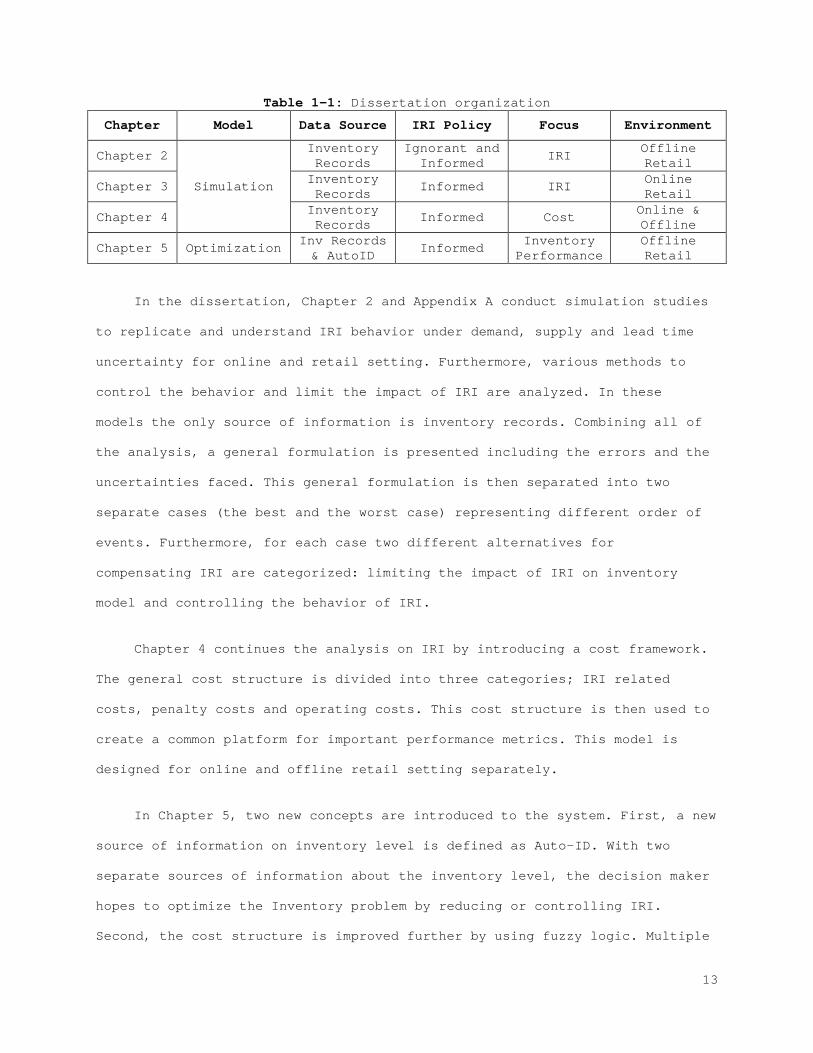
Table 1-1: Dissertation organization
Chapter Model Data Source IRI Policy Focus Environment
Chapter 2
Simulation
Inventory Records
Ignorant and Informed IRI Offline
Retail
Chapter 3 Inventory Records Informed IRI Online
Retail
Chapter 4 Inventory Records Informed Cost Online &
Offline
Chapter 5 Optimization Inv Records & AutoID Informed Inventory
Performance Offline Retail
In the dissertation, Chapter 2 and Appendix A conduct simulation studies
to replicate and understand IRI behavior under demand, supply and lead time
uncertainty for online and retail setting. Furthermore, various methods to
control the behavior and limit the impact of IRI are analyzed. In these
models the only source of information is inventory records. Combining all of
the analysis, a general formulation is presented including the errors and the
uncertainties faced. This general formulation is then separated into two
separate cases (the best and the worst case) representing different order of
events. Furthermore, for each case two different alternatives for
compensating IRI are categorized: limiting the impact of IRI on inventory
model and controlling the behavior of IRI.
Chapter 4 continues the analysis on IRI by introducing a cost framework.
The general cost structure is divided into three categories; IRI related
costs, penalty costs and operating costs. This cost structure is then used to
create a common platform for important performance metrics. This model is
designed for online and offline retail setting separately.
In Chapter 5, two new concepts are introduced to the system. First, a new
source of information on inventory level is defined as Auto-ID. With two
separate sources of information about the inventory level, the decision maker
hopes to optimize the Inventory problem by reducing or controlling IRI.
Second, the cost structure is improved further by using fuzzy logic. Multiple
13

fuzzy cost parameters are defined and then combined in a multi-objective
setting. With both sources of information the inventory problem is modeled as
an infinite horizon discounted MDP with fuzzified multi-objective. This model
is extensively analyzed to understand the optimal policy structure.
14
REFERENCES
Agrawal, V. (2001). Assessing the Benefits of Auto-ID Technology in the Consumer Goods Industry. MIT, Technical Report of the Auto ID Center.
ARTICTE, P. N. (1995). Raster Procedures for Multi-Criteria/Multi-Objective
Decisions. Photogrammetric Engineering & Remote Sensing, 61, 539-547. Atali, A., Lee, H. L., & Ozer, O. (2006). If the inventory manager knew:
value of RFID under imperfect inventory information. Stanford University.
Baudin, M. (1996). Supporting JIT production with the best wage system. IE
Solutions, 28, 30-35. Boritz, E. J. (2003). IS Practitioners' Views on Core Concepts of Information
Integrity. International Journal of Accounting Information Systems. Boxx, D. B. (1979). Selling a dead horse (or how to convince management to
initiate MRP. Production and Inventory Management, 20, 49-62. Bragg, D. J. (1984). The impact of inventory record inaccuracy on material
requirements planning systems. Columbus, Ohio: Ph.D. dissertation, Ohio State University
Buker, D. W. (1979). Performance measurement. Paper presented at the
Proceedings of the 22nd Annual International Conference, St. Louis. Carver, S. J. (1991). Integrating multi-criteria evaluation with geographical
information systems. International Journal of Geographical Information System, 5, 321-339.
Chang, H. C., Yao, J. S., & Ouyang, L. Y. (2006). Fuzzy mixture inventory
model involving fuzzy random variable lead time demand and fuzzy total demand. European Journal of Operational Research, 169, 165-180.
Chen, L. H., & Tsai, F. C. (2001). Fuzzy goal programming with different
importance and priorities. European Journal of Opertaional Research, 133, 348-556.
Covin, S. (1981). Inventory inaccuracy: one of your first hurdles. Production
and Inventory Management, 22, 13-23. DeHoratius, N., & Raman, A. (2008). Inventory record inaccuracy: an empirical
analysis. Management Science, 54, 627-641. Feiring, B. E. (1986). Linear programming: An introduction: Sage. French, R. L. (1980). Accurate work in process inventory - a critical MRP
system requirement. Production and Inventory Management, 21, 17-22. Gentry, C. R. (2005). Theft and terrorism. Chain Store Age, 81, 66--68. Iglehart, D., & Morey, R. C. (1972). Inventory systems with imperfect assest
information. Management Science, 18, 388-394.
15
Ignizio, J. P. (1985). Introduction to linear goal programming. Beverly Hills: Sage.
Kacprzyk, J., & Staniewski, P. (1982). Long term inventory policy-making
through fuzzy decision making models. Fuzzy sets and systems, 8, 117-132.
Kang, Y., & Gershwin, S. B. (2004). Information inaccuracy in inventory
systems stock loss and stockout. IIE Transactions, 37, 843-859. Kok, A. G., & Shang, K. H. (2007). Inspection and replenishment policies for
systems with inventory record inaccuracy. Manufacturing & Service Operations Management, 9, 185-205.
Krajewski, L. J., King, B. E., Ritzmann, L. P., & Wong, D. S. (1987). Kanban,
MRP and shaping the manufacturing environment. Management Science, 33, 39-57.
Lee, H., & Ozer, O. (2007). Unlocking the value of RFID. Production and
Operations Management, 16, 40-64. Lewis, C. D. (1970). Scientific Inventory Control. London: Butterworth. Mandal, N. K., Roy, T. K., & Maiti, M. (2005). Multi-objective fuzzy
inventory model with three constraints: a geometric programming approach. Fuzzy sets and systems, 150(1), 87-106.
Marler, R. T., & Arora, J. S. (2003). Review of multi-objective optimization
concepts and methods for engineering. IA, USA: University of Iowa. Millet, I. (1994). A novena to Saint Anthony, or how to find inventory by not
looking. Interfaces, 24, 69-75. Mosconi, R., Raman, A., & Zotteri, G. (2004). The impact of data quality and
zero-balance walks on retail inventory management. MA, Boston: Harvard Business School.
Naddor, E. (1966). Inventory Systems. New York: John Wiley. Park, K. S. (1987). Fuzzy set theoric interpretation of economic order
quantity. IEEE Transactions on SYstems, Man, and Cybernetics, 6, 1082-1084.
Petrovic, D., & Sweeney, E. (1994). Fuzzy knowledge-based approach to
treating uncertainty in inventory control. Computer Integrated Manufacturing Systems, 7, 147-152.
Plossl, G. W. (1977). The best investment - control, not machinery.
Production and Inventory Management, 18, 11-17. Raman, A., DeHoratius, N., & Ton, Z. (2001). The Achilles' heel of supply
chain management. Harvard Business Review, 79, 25-28. Relph, G., Brzeski, W., & Bradbear, G. (2003). First steps to Inventory
Management. IOM Control Journal, 28, 10.
16
Rinehart, R. F. (1960). Effects and causes of discrepancies in supply operations. Operations Research, 8, 543-564.
Ritzman, L. P., King, B. E., & Krajewski, L. J. (1984). Manufacturing
performance - pulling the right levers. Harvard Business Review, 62, 143-152.
Robison, J. A. (1994). Inventory vocabulary accuracy. APICS - The Performance
Advantage, 4, 40-41. Roy, T. K., & Maiti, M. (1997). A fuzzy EOQ model with demand-dependent unit
cost under limited storage capacity. European Journal of Operational Research, 99, 425-432.
Roy, T. K., & Maiti, M. (1998). Multi-objective inventory models of
deteriorating items with some constraints in a fuzzy environment. Computers & operations research, 25, 1085-1095.
Sakawa, M., & Yauchi, K. (2001). An interactive fuzzy satisficing method for
multiobjective nonconvex programming problems with fuzzy numbers through coevolutionary genetic algorithms. Systems, Man, and Cybernetics, Part B: Cybernetics, IEEE Transactions on, 31(3), 459-467.
Silver, E. A., & Peterson, R. (1985). Decision systems for inventory
management and production planning. New York: John Wiley. Steidtmann, C. (1999). The new retail technology. Discount Merchandiser, 23-
24. Ton, Z., & Raman, A. (2004). An empirical anaylsis of misplaced skus in
reatil stores. Harvard Business School. Tsou, C. S. (2008). Multi-objective inventory planning using MOPSO and
TOPSIS. Expert Systems with Applications, 35, 136-142. Vujosevic, M., Petrovic, D., & Petrovic, R. (1996). EOQ formula when
inventory cost is fuzzy. International Journal of Production Economics, 45, 499-504.
Wee, H. M., Lo, C. C., & Hsu, P. H. (2009). A multi-objective joint
replenishment inventory model of deteriorated items in a fuzzy environment. European Journal of Operational Research, 197, 620-631.
Xu, J., & Liu, Y. (2008). Multi-objective decision making model under fuzzy
random environment and its application to invenotry problems. Information Sciences, 178, 2899-2914.
Zadeh, L. A. (1965). Fuzzy sets. Information and control, 8,338-353.
17
CHAPTER 2 IRI ANALYSIS IN OFFLINE RETAILING WITH LEAD TIME AND SUPPLY
UNCERTAINTY
Inventory models are one of the widely studied topics in supply chain
management. Due to the uncertain nature of the system parameters such as
demand, supply, lead times and errors, these models are known to have a
complex structure. In practice, dealing with these uncertain factors,
satisfying the high service levels, and reaching optimal solutions at the
same time are very difficult.
Majority of the research on inventory models operate under the assumption
perfect record accuracy. According to Bensoussan et al. (2005), a limited
number of studies investigate IRI mainly due to retailers do not publicize
their lack of full inventory information, and because the information must be
inferred from surrogate measures. Moreover, the assumption of perfect
accuracy assumption greatly reduces the theoretical complexity of the
inventory problems. However, in real settings, inventory records are likely
to be incorrect. The lack of theoretical studies in this conjecture has left
practices susceptible to unrequired replenishment, unnecessary procurement
and occasional delays in supplying customers. Empirical studies try to
quantify and reveal the impact of data accuracy assumption. In Iglehart and
Morey (1972), out of 20,000 total items 25% revealed discrepancies which
corresponded roughly 4% of monthly inventory. In Raman et al. (2001) 65% of
370,000 units of inventory, did not match the physical stocks.
The objective of this dissertation is to understand the IRI concept in
the offline environment, explore the effects induced by uncertainty, and
apply methods to control the impact of IRI. In the offline retail setting,
IRI can briefly be defined as the error when the stock record is not in
18
agreement with the physical stock. Such discrepancies are generally
introduced to the system during three operations, inbound transactions,
shelving operations and outbound transactions. These errors force the system
to operate with inaccurate information and make wrong decisions, often
followed by a stock-out. The susceptibility in this setting arises from two
factors, the capabilities of technological systems and the shortcomings of
the theoretical inventory models used in the system. Hence, it is clear that
inventory policies that are more resistant to IRI and technologies that can
capture data more effectively are needed.
Lead time and supply uncertainty are extensively researched topics in
inventory management problems. However, the literature on IRI commonly
operates under the assumption that the lead time and the supply are
deterministic. This dissertation also investigates the influence of the
additional uncertainty caused by the random supply and the random lead time.
Supply uncertainty. The introduction of general random lead time mechanism
often causes disruptions in the supply chain coordination due to loss of
tractability (Bashyam & Fu, 1998). Furthermore, it enhances the stock-out
risk faced during the lead time. The supply uncertainty, on the other hand,
is often caused by two factors, random capacity and random yield of the
suppliers (Henig & Gerchak, 1990). In our study, we use simulation analyses
to model these extra uncertainties and estimating performance.
The outline of this chapter is as follows, Section 2.1 presents the
general characterization for errors under demand, supply and lead time
uncertainty. In Section 2.2 for a continuous review inventory problem,
methods for compensating the impact of IRI are examined. Also the analysis is
tested on a numerical example. Finally, in Section 2.3 a discussion about
this study is presented.
19
2.1 Model
As previously mentioned, the IRI is affected by many uncertain factors
such as random demand, random supply, and lead time, in addition to the
inventory management related errors. The complication is that the
relationship is not one sided; IRI also affects all of these factors. Various
enumerations of IRI can be found in the literature. Underlying error factors
are typically categorized based on dependent variables. In this study
however, we will categorize these error factors based on their impacts on
inventory as follows: (1) Inbound errors: Errors that occur during ordering
and receiving process; (2) Shelving errors: Errors that are due to damaged,
stolen, or expire SKUs, which cause the physical stock to change without
informing inventory records; (3) Outbound errors: Errors that occur during
check-out processes (e.g. scanning errors). When left uncorrected, these
errors will significantly lower retailer performance by increasing the stock-
out rate. According to Gruen et al. (2002) the stock-out rates on average
fall in range 5-10% which roughly corresponds to 4% of sales.
Figure 2-1 shows a typical continuous inventory behavior subject to
errors. In the considered model, the start of each period is identified as
points at which a replenishment order is given. In order to create a
generalized model, let ktx denote the amount of actual inventory and
ktx
denote the inventory record at time kt , at the replenishment order time in
period k .
20
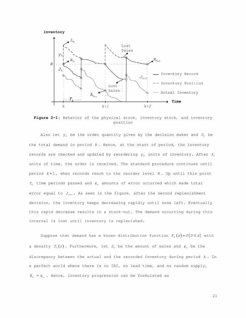
Figure 2-1: Behavior of the physical stock, inventory stock, and inventory position
Also let ky be the order quantity given by the decision maker and kD be
the total demand in period k . Hence, at the start of period, the inventory
records are checked and updated by reordering ky units of inventory. After kτ
units of time, the order is received. The standard procedure continues until
period 1k + , when records reach to the reorder level R . Up until this point
kT time periods passed and kε amounts of error occurred which made total
error equal to 1kJ + . As seen in the figure, after the second replenishment
decision, the inventory keeps decreasing rapidly until none left. Eventually
this rapid decrease results in a stock-out. The demand occurring during this
interval is lost until inventory is replenished.
Suppose that demand has a known distribution function ( ) { }DF z P D z= ≤ with
a density ( )Df z . Furthermore, let kS be the amount of sales and kε be the
discrepancy between the actual and the recorded inventory during period k . In
a perfect world where there is no IRI, no lead time, and no random supply,
k kt tx x= . Hence, inventory progression can be formulated as
21
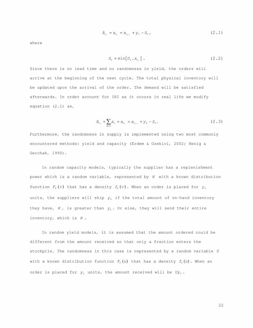
1k k kt t t k kx x x y S−
= = + − , (2.1)
where
{ }min ,kk k tS D x= . (2.2)
Since there is no lead time and no randomness in yield, the orders will
arrive at the beginning of the next cycle. The total physical inventory will
be updated upon the arrival of the order. The demand will be satisfied
afterwards. In order account for IRI as it occurs in real life we modify
equation (2.1) as,
1k k kt k t t k k
k K
x x x y Sε−
∈
+ = = + −∑ . (2.3)
Furthermore, the randomness in supply is implemented using two most commonly
encountered methods: yield and capacity (Erdem & Ozekici, 2002; Henig &
Gerchak, 1990).
In random capacity models, typically the supplier has a replenishment
power which is a random variable, represented by K with a known distribution
function ( )KF v that has a density ( )Kf v . When an order is placed for ky
units, the suppliers will ship ky if the total amount of on-hand inventory
they have, K , is greater than ky . Or else, they will send their entire
inventory, which is K .
In random yield models, it is assumed that the amount ordered could be
different from the amount received so that only a fraction enters the
stockpile. The randomness in this case is represented by a random variable U
with a known distribution function ( )UF u that has a density ( )Uf u . When an
order is placed for ky units, the amount received will be kUy .
22
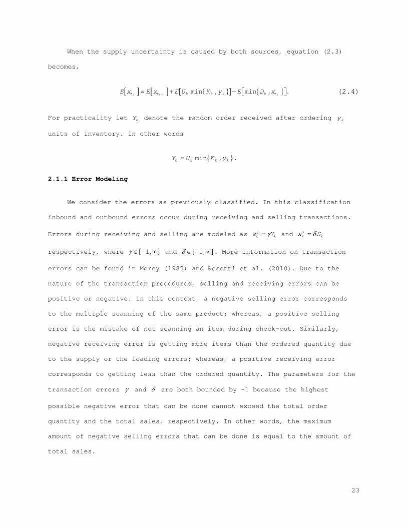
When the supply uncertainty is caused by both sources, equation (2.3)
becomes,
[ ] [ ] { }[ ] { }1
min , min ,k k kt t k k k k tE x E x E U K y E D x
−= + − . (2.4)
For practicality let kY denote the random order received after ordering ky
units of inventory. In other words
{ }min ,k kk kU KY y= .
2.1.1 Error Modeling
We consider the errors as previously classified. In this classification
inbound and outbound errors occur during receiving and selling transactions.
Errors during receiving and selling are modeled as rk kYε γ= and s
k kSε δ=
respectively, where [ ]1,γ ∈ − ∞ and [ ]1,δ ∈ − ∞ . More information on transaction
errors can be found in Morey (1985) and Rosetti et al. (2010). Due to the
nature of the transaction procedures, selling and receiving errors can be
positive or negative. In this context, a negative selling error corresponds
to the multiple scanning of the same product; whereas, a positive selling
error is the mistake of not scanning an item during check-out. Similarly,
negative receiving error is getting more items than the ordered quantity due
to the supply or the loading errors; whereas, a positive receiving error
corresponds to getting less than the ordered quantity. The parameters for the
transaction errors γ and δ are both bounded by -1 because the highest
possible negative error that can be done cannot exceed the total order
quantity and the total sales, respectively. In other words, the maximum
amount of negative selling errors that can be done is equal to the amount of
total sales.
23
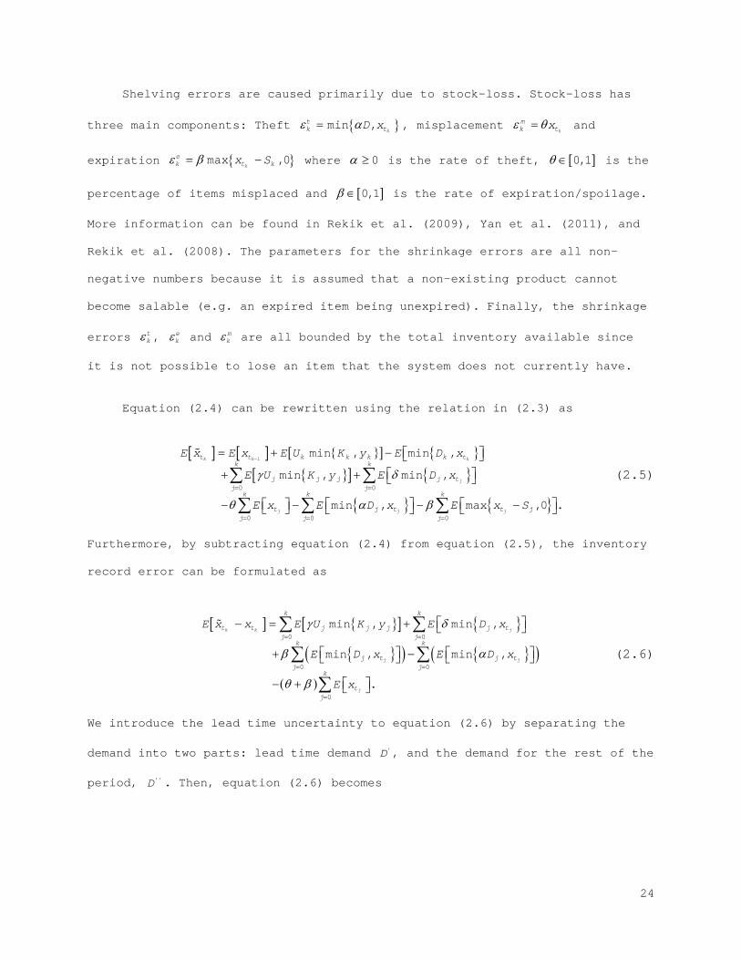
Shelving errors are caused primarily due to stock-loss. Stock-loss has
three main components: Theft { }min ,k
tk tD xε α= , misplacement
k
mk txε θ= and
expiration { }max ,0k
ek t kx Sε β= − where 0α ≥ is the rate of theft, [ ]0,1θ ∈ is the
percentage of items misplaced and [ ]0,1β ∈ is the rate of expiration/spoilage.
More information can be found in Rekik et al. (2009), Yan et al. (2011), and
Rekik et al. (2008). The parameters for the shrinkage errors are all non-
negative numbers because it is assumed that a non-existing product cannot
become salable (e.g. an expired item being unexpired). Finally, the shrinkage
errors tkε , e
kε and mkε are all bounded by the total inventory available since
it is not possible to lose an item that the system does not currently have.
Equation (2.4) can be rewritten using the relation in (2.3) as
[ ] [ ] { }[ ] { }{ }[ ] { }
{ } { }
1
0 0
0 0 0
min , min ,
min , min ,
min , max .,0
j
j j j
k k kt t k k k k tk k
j tj j
k k k
t j t tj
j j
jj
j
j
E x E x E U K y E D x
E U K y E D x
E x E D E x Sx
γ δ
θ α β
−
= =
= = =
−
= + −
+ +
− − −
∑ ∑
∑ ∑ ∑
(2.5)
Furthermore, by subtracting equation (2.4) from equation (2.5), the inventory
record error can be formulated as
[ ] { }[ ] { }
{ }( ) { }( )( )
0 0
0 0
0
min m, ,in
min m, in ,
.
k k
j
j
j
j
t t t
j t j t
t
k k
j j j jj j
k k
j jk
j
E x x E U K y E D x
E D E D x
xE
xβ
γ δ
α
θ β
= =
= =
=
+ −
− = +
− +
∑ ∑
∑ ∑
∑
(2.6)
We introduce the lead time uncertainty to equation (2.6) by separating the
demand into two parts: lead time demand 'D , and the demand for the rest of the
period, ''D . Then, equation (2.6) becomes
24
[ ] { }[ ] { }
{ } { }[ ]( ){ } { }[ ]( )
( )
0 0
0
0
0
' ''
' ''
, ,
, min ,
, m
min min
mi
in
n
min ,j
j
j
j
k t
j t j j
k k
j j j jj j
k
jk
j
j
j t j j j
t
k
jj
j
E J E U K y E D x
E D x E D Y w
D x D Y w
x Y
E E
E w
γ δ
α α
β
θ β
= =
=
=
=
+
− +
− + +
= +
+
+
+
+
∑ ∑
∑
∑
∑
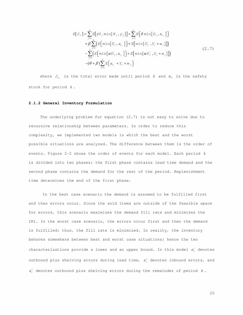
(2.7)
where ktJ is the total error made until period k and kw is the safety
stock for period k .
2.1.2 General Inventory Formulation
The underlying problem for equation (2.7) is not easy to solve due to
recursive relationship between parameters. In order to reduce this
complexity, we implemented two models in which the best and the worst
possible situations are analyzed. The difference between them is the order of
events. Figure 2-2 shows the order of events for each model. Each period k
is divided into two phases: the first phase contains lead time demand and the
second phase contains the demand for the rest of the period. Replenishment
time determines the end of the first phase.
In the best case scenario the demand is assumed to be fulfilled first
and then errors occur. Since the sold items are outside of the feasible space
for errors, this scenario maximizes the demand fill rate and minimizes the
IRI. In the worst case scenario, the errors occur first and then the demand
is fulfilled; thus, the fill rate is minimized. In reality, the inventory
behaves somewhere between best and worst case situations; hence the two
characterizations provide a lower and an upper bound. In this model 1kε denotes
outbound plus shelving errors during lead time, 2kε denotes inbound errors, and
3kε denotes outbound plus shelving errors during the remainder of period k .
25
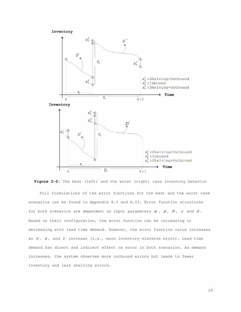
Figure 2-2: The best (left) and the worst (right) case inventory behavior
Full formulations of the error functions for the best and the worst case
scenarios can be found in Appendix A.I and A.II. Error function structures
for both scenarios are dependent on input parameters α , β , θ , γ and δ .
Based on their configuration, the error function can be increasing or
decreasing with lead time demand. However, the error function value increases
as R , w , and Y increase (i.e., more inventory elevates error). Lead time
demand has direct and indirect effect on error in both scenarios. As demand
increases, the system observes more outbound errors but leads to fewer
inventory and less shelving errors.
26
2.1.3 Numerical Study
Characterization and behavior of the developed error function are
analyzed using a case study provided by an appliance and furniture company
(The data provided ranges from 1990 - 2003). In the case study, a continuous
( ),Q R policy is utilized with ( )600,80 . Weekly demand D and lead time τ are
normally distributed with ( )250,12 and ( )21.14,0.33 respectively.
The parameters for the errors are selected from various examples in the
literature. The transaction errors are assumed to be uniformly distributed,
( )1%,1%unifδ − and ( )2%,2%unifγ − (Morey, 1985; Rosetti et al., 2010). The
shelving parameters are defined as 1%α = and 0.5%β = for theft and
misplacement, respectively (Rekik et al., 2008, 2009; Yan et al., 2011).
Over 2000 random numbers for D and τ with 5 replications are generated
to obtain the expected errors in a single period. There are seven different
sources of errors in each period. We categorize these errors into 3 types:
three of these errors are first phase errors, three of them are second phase
errors and the last one is the inbound error in between phases.
We conducted a discrete event simulation for 52 periods with 60
replications for ( ),Q R policy. It is assumed that the model starts with 0 IRI
when the inventory records and actual physical stock equal to the reorder
level. The model is depicted in Figure 2-3.
27
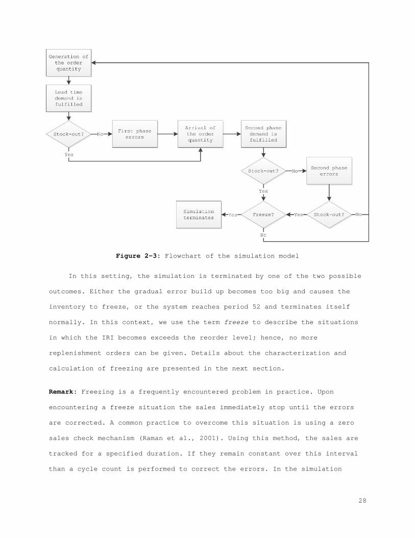
Figure 2-3: Flowchart of the simulation model
In this setting, the simulation is terminated by one of the two possible
outcomes. Either the gradual error build up becomes too big and causes the
inventory to freeze, or the system reaches period 52 and terminates itself
normally. In this context, we use the term freeze to describe the situations
in which the IRI becomes exceeds the reorder level; hence, no more
replenishment orders can be given. Details about the characterization and
calculation of freezing are presented in the next section.
Remark: Freezing is a frequently encountered problem in practice. Upon
encountering a freeze situation the sales immediately stop until the errors
are corrected. A common practice to overcome this situation is using a zero
sales check mechanism (Raman et al., 2001). Using this method, the sales are
tracked for a specified duration. If they remain constant over this interval
than a cycle count is performed to correct the errors. In the simulation
28
study, we are not implementing a correction model, hence once freezing is
observed the simulation terminates.
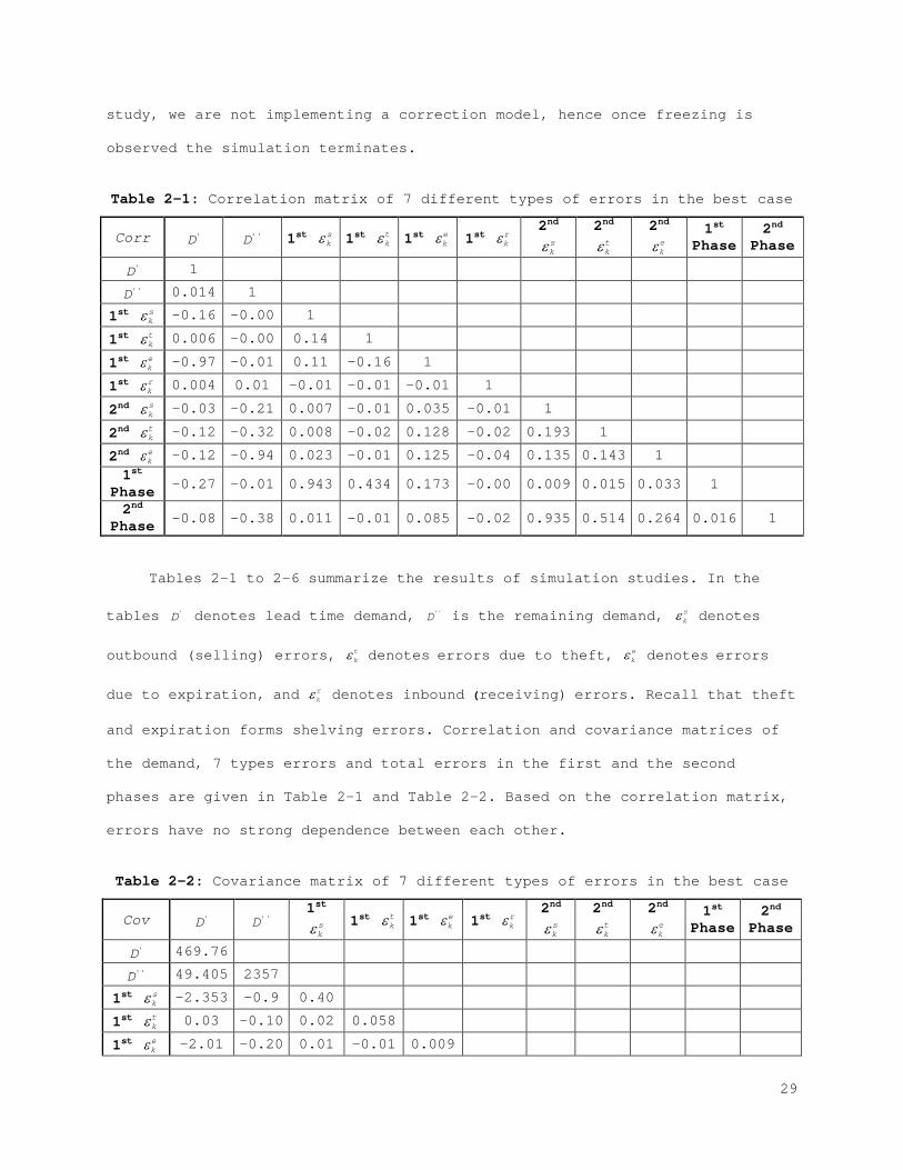
Table 2-1: Correlation matrix of 7 different types of errors in the best case
Corr 'D ''D 1st skε 1st t
kε 1st ekε 1st r
kε 2nd
skε
2nd tkε
2nd ekε
1st Phase
2nd Phase
'D 1 ''D 0.014 1
1st skε -0.16 -0.00 1
1st tkε 0.006 -0.00 0.14 1
1st ekε -0.97 -0.01 0.11 -0.16 1
1st rkε 0.004 0.01 -0.01 -0.01 -0.01 1
2nd skε -0.03 -0.21 0.007 -0.01 0.035 -0.01 1
2nd tkε -0.12 -0.32 0.008 -0.02 0.128 -0.02 0.193 1
2nd ekε -0.12 -0.94 0.023 -0.01 0.125 -0.04 0.135 0.143 1
1st Phase -0.27 -0.01 0.943 0.434 0.173 -0.00 0.009 0.015 0.033 1
2nd Phase -0.08 -0.38 0.011 -0.01 0.085 -0.02 0.935 0.514 0.264 0.016 1
Tables 2-1 to 2-6 summarize the results of simulation studies. In the
tables 'D denotes lead time demand, ''D is the remaining demand, skε denotes
outbound (selling) errors, tkε denotes errors due to theft, e
kε denotes errors
due to expiration, and rkε denotes inbound (receiving) errors. Recall that theft
and expiration forms shelving errors. Correlation and covariance matrices of
the demand, 7 types errors and total errors in the first and the second
phases are given in Table 2-1 and Table 2-2. Based on the correlation matrix,
errors have no strong dependence between each other.
Table 2-2: Covariance matrix of 7 different types of errors in the best case
Cov 'D ''D 1st
skε 1st t
kε 1st ekε 1st r
kε 2nd
skε
2nd tkε
2nd ekε
1st Phase
2nd Phase
'D 469.76 ''D 49.405 2357
1st skε -2.353 -0.9 0.40
1st tkε 0.03 -0.10 0.02 0.058
1st ekε -2.01 -0.20 0.01 -0.01 0.009
29
Cov 'D ''D 1st
skε 1st t
kε 1st ekε 1st r
kε 2nd
skε
2nd tkε
2nd ekε
1st Phase
2nd Phase
1st rkε 0.348 9.61 -0.01 -0.01 -0.01 11.889
2nd skε -4.295 -175 0.02 -0.01 0.018 -0.261 29.3
2nd tkε -5.67 -105 0.01 -0.01 0.025 -0.184 2.21 4.457
2nd ekε -1.67 -91.2 0.01 -0.00 0.007 -0.09 0.46 0.191 0.396
1st Phase -4.335 -1.2 0.43 0.075 0.011 -0.022 0.03 0.023 0.015 0.525
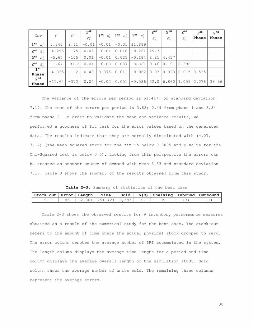
2nd Phase -11.64 -372 0.04 -0.02 0.051 -0.536 32.0 6.860 1.051 0.076 39.96
The variance of the errors per period is 51.417, or standard deviation
7.17. The mean of the errors per period is 3.83; 0.49 from phase 1 and 3.34
from phase 2. In order to validate the mean and variance results, we
performed a goodness of fit test for the error values based on the generated
data. The results indicate that they are normally distributed with (4.07,
7.12) (The mean squared error for the fit is below 0.0005 and p-value for the
Chi-Squared test is below 0.5). Looking from this perspective the errors can
be treated as another source of demand with mean 3.83 and standard deviation
7.17. Table 3 shows the summary of the results obtained from this study.
Table 2-3: Summary of statistics of the best case
Stock-out Error Length Time Sold n(R) Shelving Inbound Outbound 9 85 12.301 251.421 9,595 36 89 (3) (1)
Table 2-3 shows the observed results for 9 inventory performance measures
obtained as a result of the numerical study for the best case. The stock-out
refers to the amount of time where the actual physical stock dropped to zero.
The error column denotes the average number of IRI accumulated in the system.
The length column displays the average time length for a period and time
column displays the average overall length of the simulation study. Sold
column shows the average number of units sold. The remaining three columns
represent the average errors.
30
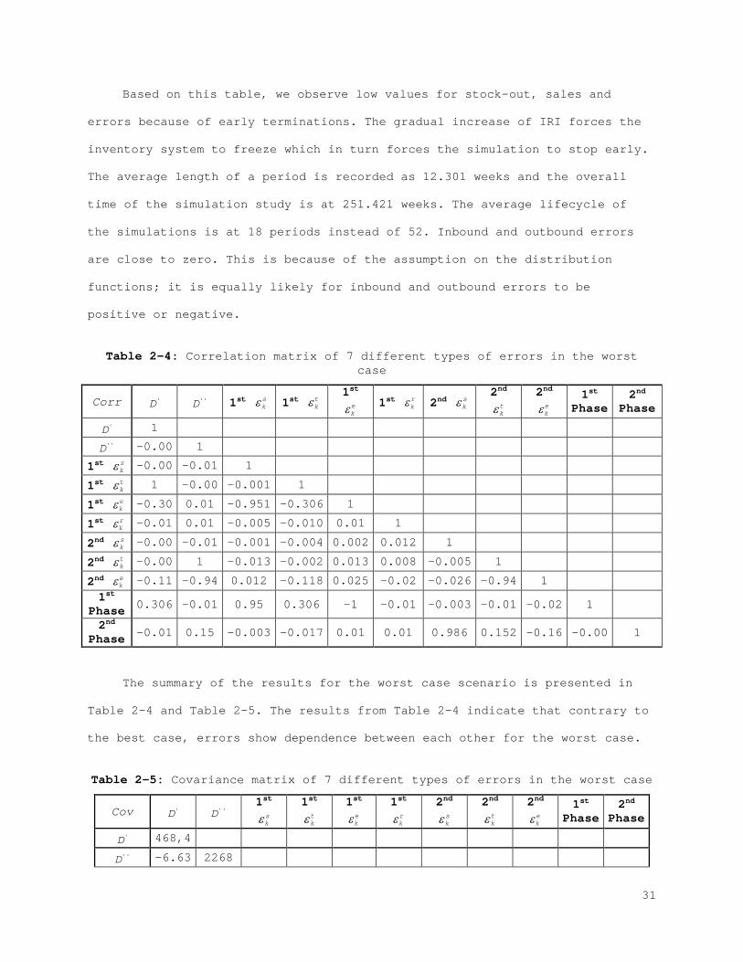
Based on this table, we observe low values for stock-out, sales and
errors because of early terminations. The gradual increase of IRI forces the
inventory system to freeze which in turn forces the simulation to stop early.
The average length of a period is recorded as 12.301 weeks and the overall
time of the simulation study is at 251.421 weeks. The average lifecycle of
the simulations is at 18 periods instead of 52. Inbound and outbound errors
are close to zero. This is because of the assumption on the distribution
functions; it is equally likely for inbound and outbound errors to be
positive or negative.
Table 2-4: Correlation matrix of 7 different types of errors in the worst case
Corr 'D ''D 1st skε 1st t
kε 1st
ekε 1st r
kε 2nd skε
2nd tkε
2nd ekε
1st Phase
2nd Phase
'D 1 ''D -0.00 1
1st skε -0.00 -0.01 1
1st tkε 1 -0.00 -0.001 1
1st ekε -0.30 0.01 -0.951 -0.306 1
1st rkε -0.01 0.01 -0.005 -0.010 0.01 1
2nd skε -0.00 -0.01 -0.001 -0.004 0.002 0.012 1
2nd tkε -0.00 1 -0.013 -0.002 0.013 0.008 -0.005 1
2nd ekε -0.11 -0.94 0.012 -0.118 0.025 -0.02 -0.026 -0.94 1
1st Phase 0.306 -0.01 0.95 0.306 -1 -0.01 -0.003 -0.01 -0.02 1
2nd Phase -0.01 0.15 -0.003 -0.017 0.01 0.01 0.986 0.152 -0.16 -0.00 1
The summary of the results for the worst case scenario is presented in
Table 2-4 and Table 2-5. The results from Table 2-4 indicate that contrary to
the best case, errors show dependence between each other for the worst case.
Table 2-5: Covariance matrix of 7 different types of errors in the worst case
Cov 'D ''D 1st
skε
1st tkε
1st ekε
1st rkε
2nd skε
2nd tkε
2nd ekε
1st Phase
2nd Phase
'D 468,4 ''D -6.63 2268
31
Cov 'D ''D 1st
skε
1st tkε
1st ekε
1st rkε
2nd skε
2nd tkε
2nd ekε
1st Phase
2nd Phase
1st skε -0.01 -1.34 0.451
1st tkε 4.68 -0.06 -0.00 0.046
1st ekε -0.02 0.007 -0.00 -0.00 0.00
1st r
kε -0.76 4.548 -0.01 -0.01 0.00 11.89 2nd s
kε -0.55 -4.18 -0.01 -0.00 0.00 0.258 33.78 2nd t
kε -0.06 226.8 -0.01 -0.00 0.00 0.045 -0.04 2.268
2nd ekε -1.57 -87.4 0.004 -0.01 0.00 -0.05 -0.09 -0.87 0.379
1st Phase 4.649 -1.40 0.448 0.046 -
0.00 -0.01 -0.01 -0.01 -0.01 0.49
2nd
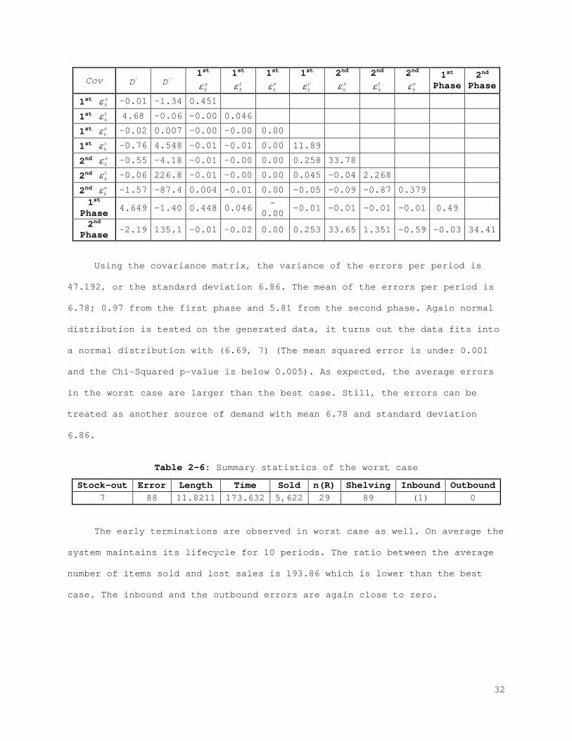
Phase -2.19 135.1 -0.01 -0.02 0.00 0.253 33.65 1.351 -0.59 -0.03 34.41
Using the covariance matrix, the variance of the errors per period is
47.192, or the standard deviation 6.86. The mean of the errors per period is
6.78; 0.97 from the first phase and 5.81 from the second phase. Again normal
distribution is tested on the generated data, it turns out the data fits into
a normal distribution with (6.69, 7) (The mean squared error is under 0.001
and the Chi-Squared p-value is below 0.005). As expected, the average errors
in the worst case are larger than the best case. Still, the errors can be
treated as another source of demand with mean 6.78 and standard deviation
6.86.
Table 2-6: Summary statistics of the worst case
Stock-out Error Length Time Sold n(R) Shelving Inbound Outbound 7 88 11.8211 173.632 5,622 29 89 (1) 0
The early terminations are observed in worst case as well. On average the
system maintains its lifecycle for 10 periods. The ratio between the average
number of items sold and lost sales is 193.86 which is lower than the best
case. The inbound and the outbound errors are again close to zero.
32
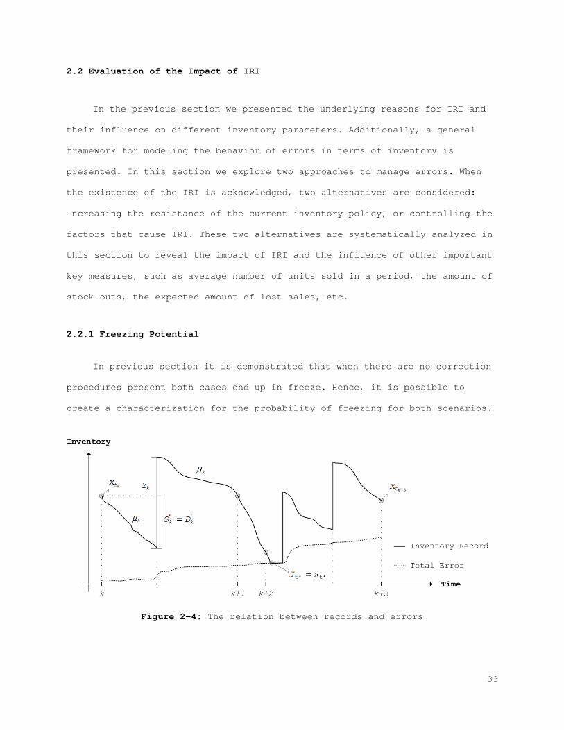
2.2 Evaluation of the Impact of IRI
In the previous section we presented the underlying reasons for IRI and
their influence on different inventory parameters. Additionally, a general
framework for modeling the behavior of errors in terms of inventory is
presented. In this section we explore two approaches to manage errors. When
the existence of the IRI is acknowledged, two alternatives are considered:
Increasing the resistance of the current inventory policy, or controlling the
factors that cause IRI. These two alternatives are systematically analyzed in
this section to reveal the impact of IRI and the influence of other important
key measures, such as average number of units sold in a period, the amount of
stock-outs, the expected amount of lost sales, etc.
2.2.1 Freezing Potential
In previous section it is demonstrated that when there are no correction
procedures present both cases end up in freeze. Hence, it is possible to
create a characterization for the probability of freezing for both scenarios.
Figure 2-4: The relation between records and errors
33
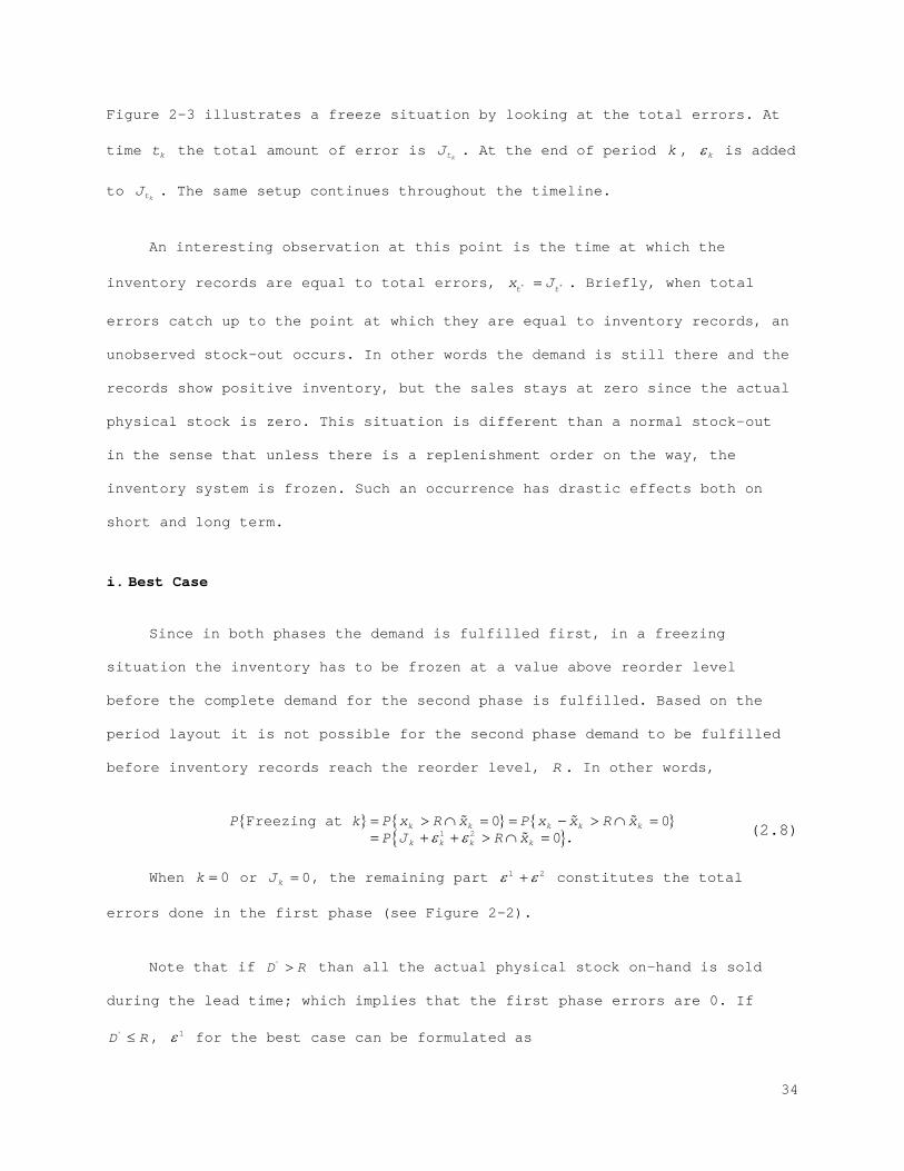
Figure 2-3 illustrates a freeze situation by looking at the total errors. At
time kt the total amount of error is ktJ . At the end of period k , kε is added
to ktJ . The same setup continues throughout the timeline.
An interesting observation at this point is the time at which the
inventory records are equal to total errors, * *t tx J= . Briefly, when total
errors catch up to the point at which they are equal to inventory records, an
unobserved stock-out occurs. In other words the demand is still there and the
records show positive inventory, but the sales stays at zero since the actual
physical stock is zero. This situation is different than a normal stock-out
in the sense that unless there is a replenishment order on the way, the
inventory system is frozen. Such an occurrence has drastic effects both on
short and long term.
i. Best Case
Since in both phases the demand is fulfilled first, in a freezing
situation the inventory has to be frozen at a value above reorder level
before the complete demand for the second phase is fulfilled. Based on the
period layout it is not possible for the second phase demand to be fulfilled
before inventory records reach the reorder level, R . In other words,
{ } { } { }{ }1 2
Freezing at 0 00 .
k k k k k
k k k k
P k P x R x P x x R xP R xJ ε ε
= > ∩ = = − > ∩ == + + > ∩ =
(2.8)
When 0k = or 0kJ = , the remaining part 1 2ε ε+ constitutes the total
errors done in the first phase (see Figure 2-2).
Note that if 'D R> than all the actual physical stock on-hand is sold
during the lead time; which implies that the first phase errors are 0. If
'D R≤ , 1ε for the best case can be formulated as
34
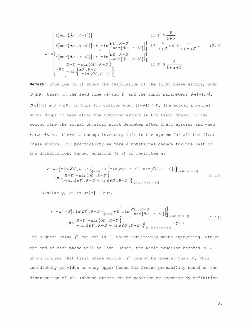
{ }[ ]
{ }[ ] { }{ }{ }[ ] { }{ }
{ }
{ }{ }
' ' '
' '' ' '
' '
1 ' '' '
' '
'' ' '
' '
' '
min , if 1
,min , min if min , 1 1
,min , min min ,
if min ,1,
min min ,
RE D R D D
R RD R DE D R D E DD R D
D R DE D R D E D R D
RDR D D R D
E D R DD R D
δδ
αδ δ δ α δε αδ δ
δα δβ α
δ
− > + − − + < ≤ − − + + +
= − − + − − ≤− − −
+ + + −− − −
. (2.9)
Remark: Equation (2.9) shows the calculation of the first phase errors, when
'D R≤ , based on the lead time demand 'D and the input parameters [ ]1,δ ∈ − ∞ ,
[ ]0,1β ∈ and 0α ≥ . In this formulation when ( ) '1 D Rδ+ > , the actual physical
stock drops to zero after the outbound errors in the first phase; in the
second line the actual physical stock depletes after theft errors; and when
( ) '1 D Rα δ+ + ≤ there is enough inventory left in the system for all the first
phase errors. For practicality we make a notational change for the rest of
the dissertation. Hence, equation (2.9) is rewritten as
{ }[ ]{ } { }{ } ( ){ }{ }
{ }{ } ( ){ }
' ' '
' '
1 ' ' ' ' ' '
1' ' '
' ' ' '
1
min , min , min ,
min ,.
min , min ,
D R D R D R
D R D R
E D R D E D R D D R D
R D D R DE
D R D D R D
δ
α δ
ε δ α δδβ α δ
≤ + ≤ ∩ ≤
+ + ≤ ∩ ≤
= − + − − − − − − + − − − −
(2.10)
Similarly, 2ε is [ ]E Yγ . Thus,
{ }[ ]{ } { }{ }( ){ }
{ }{ }{ } ( ){ }
[ ]
'' '
' '
' '1 2 ' '
' '
1' ' '
' ' ' '
1
,min , min min ,
min ,.
min , min ,
D RD R D R
D R D R
D R DE D R D E D R D
R D D R DE E Y
D R D D R D
δ
α δ
αε ε δ δδβ γα δ
≤+ ≤ ∩ ≤
+ + ≤ ∩ ≤
− + = − + − − − − − + + − − − −
(2.11)
The highest value β can get is 1, which intuitively means everything left at
the end of each phase will be lost. Hence, the whole equation becomes 'R D− ,
which implies that first phase errors, 1ε cannot be greater than R , This
immediately provides an easy upper bound for freeze probability based on the
distribution of 2ε . Inbound errors can be positive or negative by definition.
35
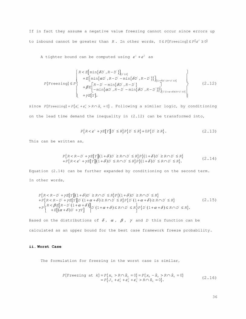
If in fact they assume a negative value freezing cannot occur since errors up
to inbound cannot be greater than R . In other words, { } { }20 Freezing 0P P ε≤ ≤ ≥
A tighter bound can be computed using 1 2ε ε+ as
{ }
{ }[ ]{ }{ }{ } ( ){ }
{ }{ }{ } ( ){ }
[ ]
'
' '
' '
' '
' ' ' '
1' ' '
' ' ' '
1
min ,
min , min ,Freezing min ,
min , min ,
.
D R
D R D R
D R D R
R E D R D
E D R D D R DP P R D D R D
ED R D D R D
E Y
δ
α δ
δα δ
δβ α δγ
≤
+ ≤ ∩ ≤
+ + ≤ ∩ ≤
< − + − − − ≤ − − − + − − − −
+
(2.12)
since { } { }1 2Freezing 0k k kP P R xε ε= + > ∩ = . Following a similar logic, by conditioning
on the lead time demand the inequality in (2.12) can be transformed into,
[ ]{ } { } { }1 ' ' '0P R E Y D R P D R P D Rε γ< + ≤ ≤ + ≥ . (2.13)
This can be written as,
[ ] ( ){ } ( ){ }[ ] ( ){ } ( ){ }
' ' ' ' '
1 ' ' ' '
1 11 1 .
P R R D E Y D R D R P D R D RP R E Y D R D R P D R D R
γ δ δε γ δ δ
< − + + ≥ ∩ ≤ + ≥ ∩ ≤+ < + + ≤ ∩ ≤ + ≤ ∩ ≤
(2.14)
Equation (2.14) can be further expanded by conditioning on the second term.
In other words,
[ ] ( ){ } ( ){ }[ ] ( ){ } ( ){ }( )[ ]
( )[ ] ( ) ( ){ }
' ' ' ' '
' ' ' ' '
'' ' ' '
'
1 11 1
11 1 .
P R R D E Y D R D R P D R D RP R R D E Y D R D R P D R D R
R E R DP D R D R P D R D R
E D Y
γ δ δγ α δ α δ
β α δ α δ α δα δ γ
< − + + ≥ ∩ ≤ + ≥ ∩ ≤+ < − + + + ≥ ∩ ≤ + + ≥ ∩ ≤
< − + + + + + ≤ ∩ ≤ + + ≤ ∩ ≤ + + +
(2.15)
Based on the distributions of δ , α , β , γ and D this function can be
calculated as an upper bound for the best case framework freeze probability.
ii. Worst Case
The formulation for freezing in the worst case is similar,
{ } { } { }{ }1 2 3
Freezing at 0 00 .
k k k k k
k k k k k
P k P x R x P x x R xP J R xε ε ε
= > ∩ = = − > ∩ == + + + > ∩ =
(2.16)
36
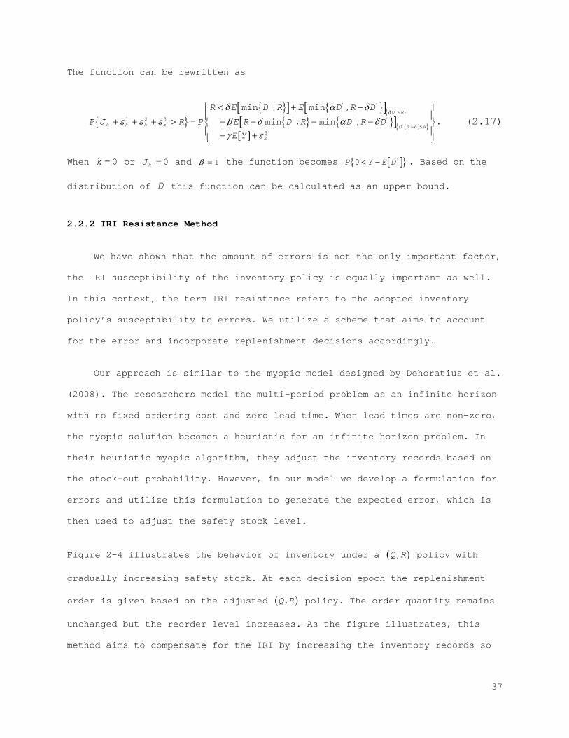
The function can be rewritten as
{ }{ }[ ] { }[ ]{ }
{ } { }[ ] ( ){ }[ ]
'
'
' ' '
1 2 3 ' ' '
3
min , min ,
min , min ,D R
k k k k D R
k
R E D R E D R D
P J R P E R D R D R D
E Y
δ
α δ
δ α δε ε ε β δ α δ
γ ε
≤
+ ≤
< + − + + + > = + − − − + +
. (2.17)
When 0k = or 0kJ = and 1β = the function becomes [ ]{ }'0P Y E D< − . Based on the
distribution of D this function can be calculated as an upper bound.
2.2.2 IRI Resistance Method
We have shown that the amount of errors is not the only important factor,
the IRI susceptibility of the inventory policy is equally important as well.
In this context, the term IRI resistance refers to the adopted inventory
policy’s susceptibility to errors. We utilize a scheme that aims to account
for the error and incorporate replenishment decisions accordingly.
Our approach is similar to the myopic model designed by Dehoratius et al.
(2008). The researchers model the multi-period problem as an infinite horizon
with no fixed ordering cost and zero lead time. When lead times are non-zero,
the myopic solution becomes a heuristic for an infinite horizon problem. In
their heuristic myopic algorithm, they adjust the inventory records based on
the stock-out probability. However, in our model we develop a formulation for
errors and utilize this formulation to generate the expected error, which is
then used to adjust the safety stock level.
Figure 2-4 illustrates the behavior of inventory under a ( ),Q R policy with
gradually increasing safety stock. At each decision epoch the replenishment
order is given based on the adjusted ( ),Q R policy. The order quantity remains
unchanged but the reorder level increases. As the figure illustrates, this
method aims to compensate for the IRI by increasing the inventory records so
37
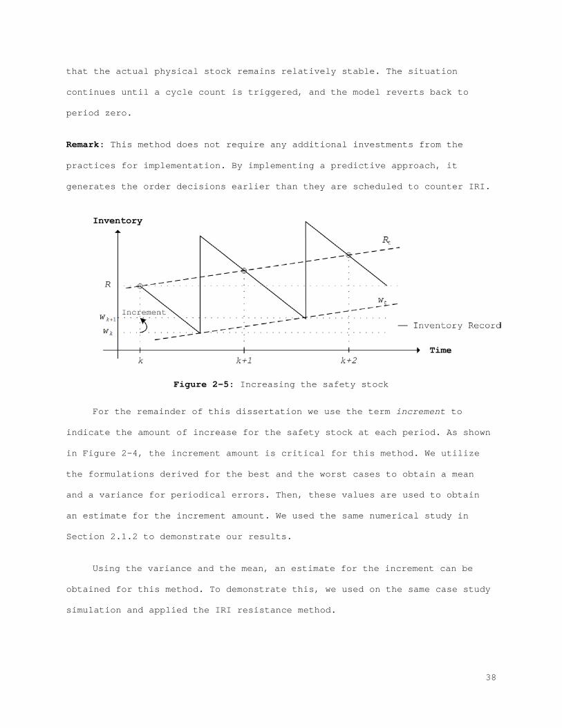
that the actual physical stock remains relatively stable. The situation
continues until a cycle count is triggered, and the model reverts back to
period zero.
Remark: This method does not require any additional investments from the
practices for implementation. By implementing a predictive approach, it
generates the order decisions earlier than they are scheduled to counter IRI.
Figure 2-5: Increasing the safety stock
For the remainder of this dissertation we use the term increment to
indicate the amount of increase for the safety stock at each period. As shown
in Figure 2-4, the increment amount is critical for this method. We utilize
the formulations derived for the best and the worst cases to obtain a mean
and a variance for periodical errors. Then, these values are used to obtain
an estimate for the increment amount. We used the same numerical study in
Section 2.1.2 to demonstrate our results.
Using the variance and the mean, an estimate for the increment can be
obtained for this method. To demonstrate this, we used on the same case study
simulation and applied the IRI resistance method.
38
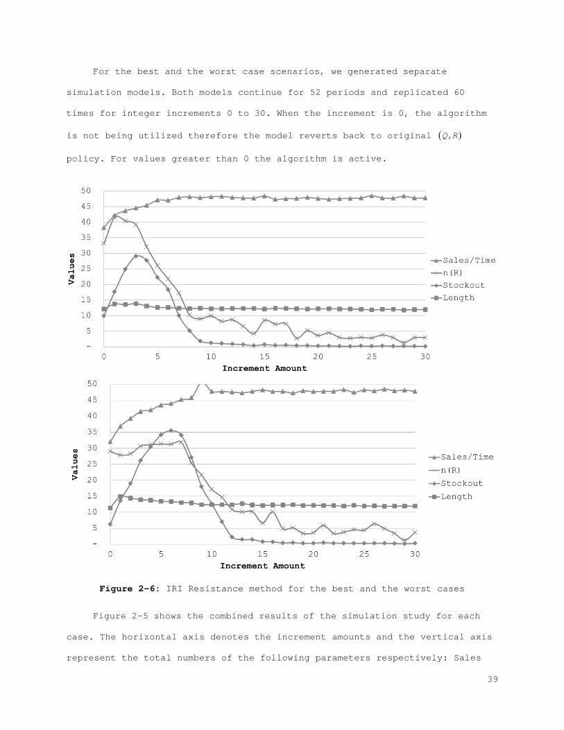
For the best and the worst case scenarios, we generated separate
simulation models. Both models continue for 52 periods and replicated 60
times for integer increments 0 to 30. When the increment is 0, the algorithm
is not being utilized therefore the model reverts back to original ( ),Q R
policy. For values greater than 0 the algorithm is active.
Figure 2-6: IRI Resistance method for the best and the worst cases
Figure 2-5 shows the combined results of the simulation study for each
case. The horizontal axis denotes the increment amounts and the vertical axis
represent the total numbers of the following parameters respectively: Sales
39
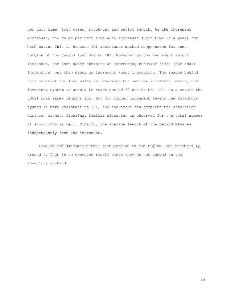
per unit time, lost sales, stock-out and period length. As the increment
increases, the sales per unit time also increases (unit time is a week) for
both cases. This is because IRI resistance method compensates for some
portion of the demand lost due to IRI. Moreover as the increment amount
increases, the lost sales exhibits an increasing behavior first (for small
increments) but then drops as increment keeps increasing. The reason behind
this behavior for lost sales is freezing. For smaller increment levels, the
inventory system is unable to reach period 52 due to the IRI. As a result the
total lost sales remains low. But for bigger increment levels the inventory
system is more resistant to IRI, and therefore can complete the simulation
duration without freezing. Similar situation is observed for the total number
of stock-outs as well. Finally, the average length of the period behaves
independently from the increment.
Inbound and Outbound errors (not present in the figure) act erratically
around 0. That is an expected result since they do not depend on the
inventory on-hand.
40
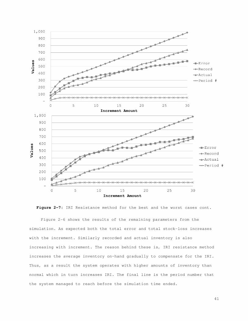
Figure 2-7: IRI Resistance method for the best and the worst cases cont.
Figure 2-6 shows the results of the remaining parameters from the
simulation. As expected both the total error and total stock-loss increases
with the increment. Similarly recorded and actual inventory is also
increasing with increment. The reason behind these is, IRI resistance method
increases the average inventory on-hand gradually to compensate for the IRI.
Thus, as a result the system operates with higher amounts of inventory than
normal which in turn increases IRI. The final line is the period number that
the system managed to reach before the simulation time ended.
41
According to Figure 2-6, there is a break point in the graphs where the
slopes changes. Also based on the simulation results higher increment levels
hurt the system more than it benefits. Therefore, there is a range where the
increment works best. Depending on preference (due to line of business),
certain parameters can be chosen and the increments that maximize or minimize
those values can be selected.
2.2.3 Error Control and Correction Method
One of the fundamental methods of error control is counting full physical
inventory. This is a process where the entire inventory is reckoned
physically (Iglehart & Morey, 1972; Opolon, 2010; Young & Nie, 1992).
However, this procedure is long and costly, especially if there is a large
number of inventory.
The literature on cycle counting and inventory auditing is vast (Iglehart
& Morey, 1972; Kok & Shang, 2007; Kumar & Arora, 1991; Meyer, 1990; Rosetti
et al., 2010; Young & Nie, 1992). While considering cycle counting practices
there are several issues to be discussed. Kok and Shang (2007) present
detailed analysis about cycle counting and consider many key aspects. The
first aspect is the trade-off between inspection frequency and IRI related
costs. The more frequent the cycle counts are, the lower the IRI is. Hence,
choosing an appropriate mechanism to determine the frequency is important. On
the other hand, inspection policies directly affect the amount of inventory
stored which in turn affects the replenishment policy. It is beneficial to
choose a replenishment policy while considering the inspection frequency.
Additionally, the effectiveness of the cycle count itself is crucial since
this process is prone to errors as well.
42
Remark: This method does not require any additional investments from the
practices for implementation. However, it includes a counting cost based on
the setup of the business and the magnitude of on-hand inventory.
As repeatedly mentioned in literature, the predominant factors for
determining the frequency of cycle counting are costs and disruptions
associated with it. Apart from these, there are other key measures that can
determine the effectiveness of the counting mechanism: lead time, amount of
expected error correction, triggering condition, amount of expected lost
sales and IRI. Our model focuses on these key metrics rather than a cost
based structure. It is assumed that the correction procedures are done error
free.
Determining the best possible triggering condition is not an easy task.
In our study we utilize the relation between the lead time sales and the
expected demand during lead time to configure a trigger mechanism. In this
relation, the expected lead time demand is a known value and the lead time
sales is an observed value. The logic behind this trigger mechanism is: If
the lead time sales is considerably lower than the expected demand during
lead time, then it can be concluded that the system contains high amounts of
IRI. However, determining the sensitivity of the trigger mechanism still
remains as a daunting issue. To overcome this burden we inserted a modifier,
called the trigger value. The main purpose of the trigger value is to adjust
the expected demand during lead time. Via this method we can effectively
change the sensitivity of the trigger mechanism.
Remark: In this context, sensitivity of the trigger mechanism determines
how often cycle counts are triggered. If the mechanism has high (or low)
sensitivity to IRI than higher (or lower) number of cycle counts will be
observed.
43
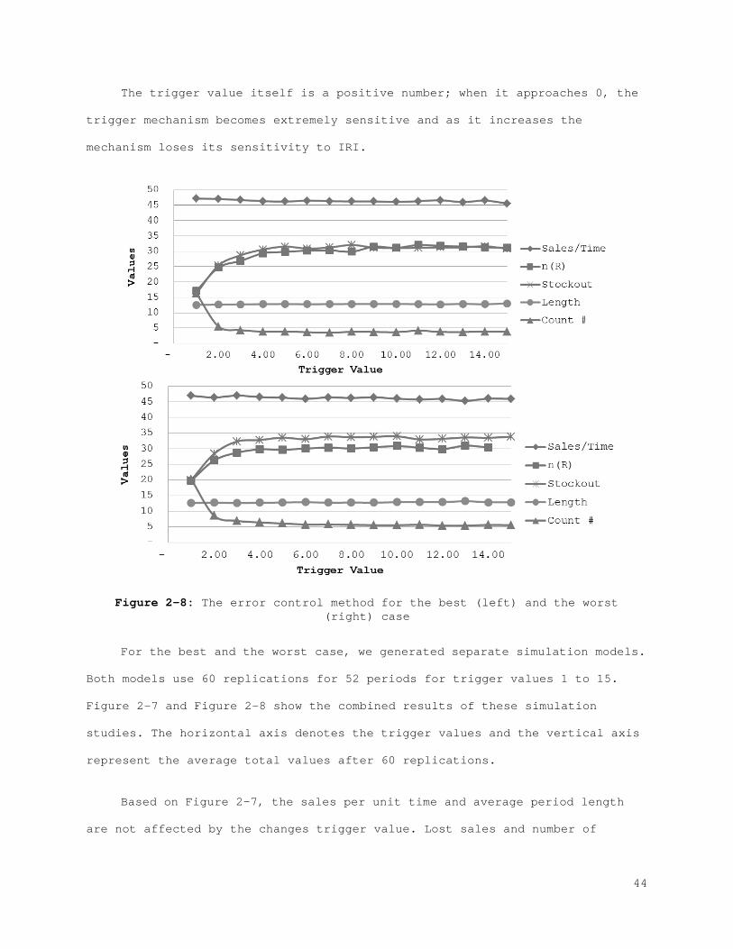
The trigger value itself is a positive number; when it approaches 0, the
trigger mechanism becomes extremely sensitive and as it increases the
mechanism loses its sensitivity to IRI.
Figure 2-8: The error control method for the best (left) and the worst (right) case
For the best and the worst case, we generated separate simulation models.
Both models use 60 replications for 52 periods for trigger values 1 to 15.
Figure 2-7 and Figure 2-8 show the combined results of these simulation
studies. The horizontal axis denotes the trigger values and the vertical axis
represent the average total values after 60 replications.
Based on Figure 2-7, the sales per unit time and average period length
are not affected by the changes trigger value. Lost sales and number of
44
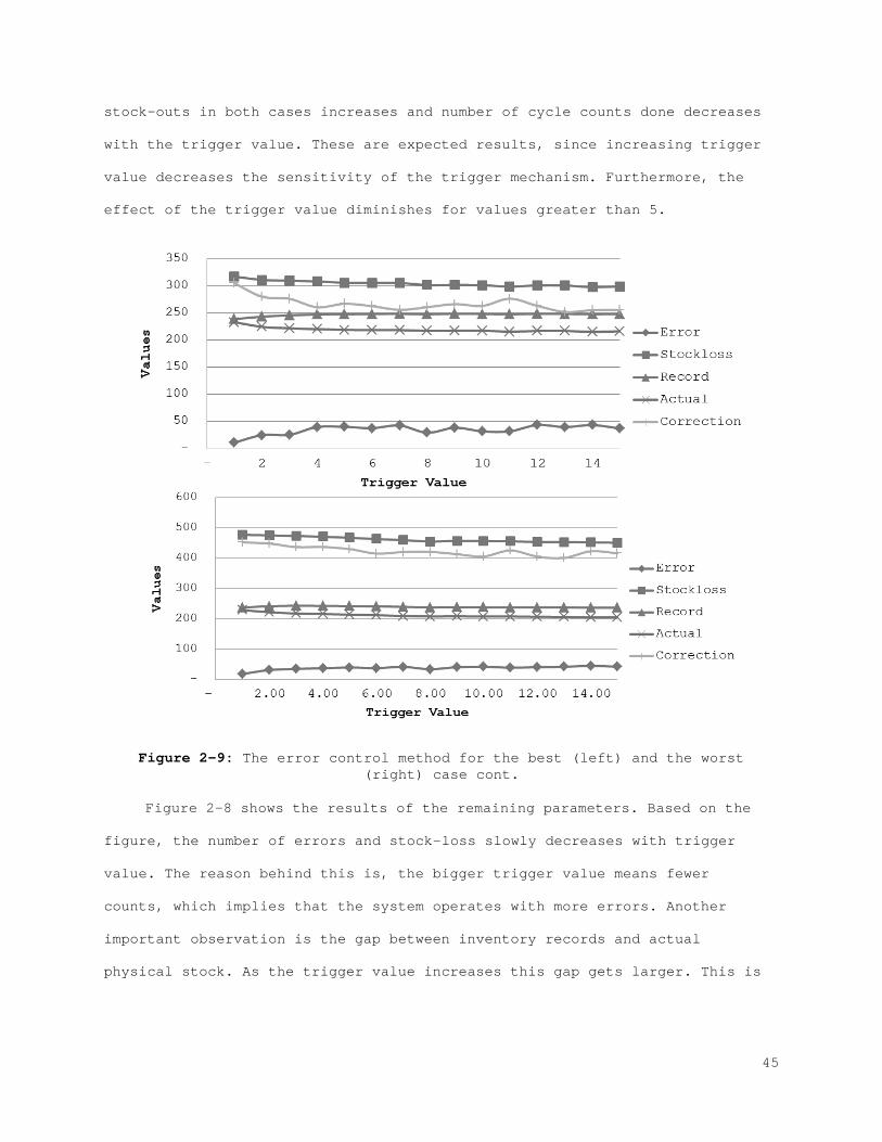
stock-outs in both cases increases and number of cycle counts done decreases
with the trigger value. These are expected results, since increasing trigger
value decreases the sensitivity of the trigger mechanism. Furthermore, the
effect of the trigger value diminishes for values greater than 5.
Figure 2-9: The error control method for the best (left) and the worst (right) case cont.
Figure 2-8 shows the results of the remaining parameters. Based on the
figure, the number of errors and stock-loss slowly decreases with trigger
value. The reason behind this is, the bigger trigger value means fewer
counts, which implies that the system operates with more errors. Another
important observation is the gap between inventory records and actual
physical stock. As the trigger value increases this gap gets larger. This is
45
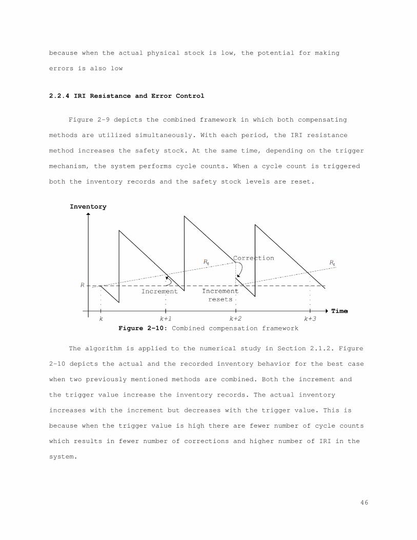
because when the actual physical stock is low, the potential for making
errors is also low
2.2.4 IRI Resistance and Error Control
Figure 2-9 depicts the combined framework in which both compensating
methods are utilized simultaneously. With each period, the IRI resistance
method increases the safety stock. At the same time, depending on the trigger
mechanism, the system performs cycle counts. When a cycle count is triggered
both the inventory records and the safety stock levels are reset.
Figure 2-10: Combined compensation framework
The algorithm is applied to the numerical study in Section 2.1.2. Figure
2-10 depicts the actual and the recorded inventory behavior for the best case
when two previously mentioned methods are combined. Both the increment and
the trigger value increase the inventory records. The actual inventory
increases with the increment but decreases with the trigger value. This is
because when the trigger value is high there are fewer number of cycle counts
which results in fewer number of corrections and higher number of IRI in the
system.
46
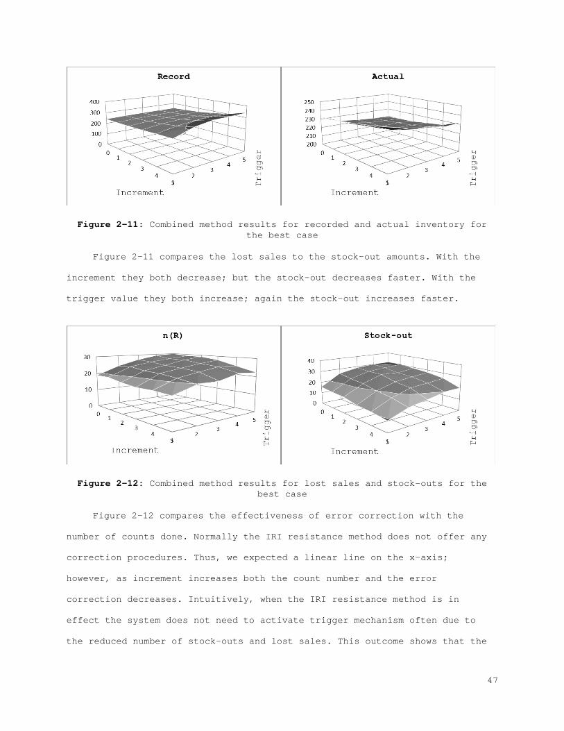
Figure 2-11: Combined method results for recorded and actual inventory for the best case
Figure 2-11 compares the lost sales to the stock-out amounts. With the
increment they both decrease; but the stock-out decreases faster. With the
trigger value they both increase; again the stock-out increases faster.
Figure 2-12: Combined method results for lost sales and stock-outs for the best case
Figure 2-12 compares the effectiveness of error correction with the
number of counts done. Normally the IRI resistance method does not offer any
correction procedures. Thus, we expected a linear line on the x-axis;
however, as increment increases both the count number and the error
correction decreases. Intuitively, when the IRI resistance method is in
effect the system does not need to activate trigger mechanism often due to
the reduced number of stock-outs and lost sales. This outcome shows that the
47
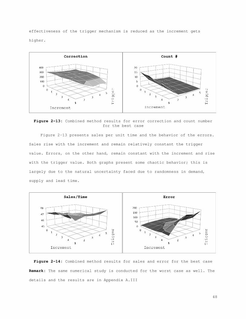
effectiveness of the trigger mechanism is reduced as the increment gets
higher.
Figure 2-13: Combined method results for error correction and count number for the best case
Figure 2-13 presents sales per unit time and the behavior of the errors.
Sales rise with the increment and remain relatively constant the trigger
value. Errors, on the other hand, remain constant with the increment and rise
with the trigger value. Both graphs present some chaotic behavior; this is
largely due to the natural uncertainty faced due to randomness in demand,
supply and lead time.
Figure 2-14: Combined method results for sales and error for the best case
Remark: The same numerical study is conducted for the worst case as well. The
details and the results are in Appendix A.III
48
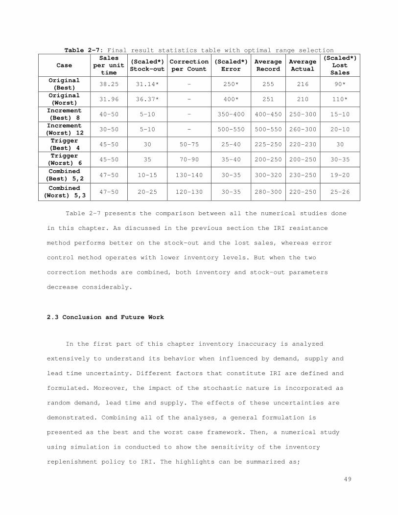
Table 2-7: Final result statistics table with optimal range selection
Case Sales
per unit time
(Scaled*) Stock-out
Correction per Count
(Scaled*) Error
Average Record
Average Actual
(Scaled*) Lost Sales
Original (Best) 38.25 31.14* - 250* 255 216 90*
Original (Worst) 31.96 36.37* - 400* 251 210 110*
Increment (Best) 8 40-50 5-10 - 350-400 400-450 250-300 15-10
Increment (Worst) 12 30-50 5-10 - 500-550 500-550 260-300 20-10
Trigger (Best) 4 45-50 30 50-75 25-40 225-250 220-230 30
Trigger (Worst) 6 45-50 35 70-90 35-40 200-250 200-250 30-35
Combined (Best) 5,2 47-50 10-15 130-140 30-35 300-320 230-250 19-20
Combined (Worst) 5,3 47-50 20-25 120-130 30-35 280-300 220-250 25-26
Table 2-7 presents the comparison between all the numerical studies done
in this chapter. As discussed in the previous section the IRI resistance
method performs better on the stock-out and the lost sales, whereas error
control method operates with lower inventory levels. But when the two
correction methods are combined, both inventory and stock-out parameters
decrease considerably.
2.3 Conclusion and Future Work
In the first part of this chapter inventory inaccuracy is analyzed
extensively to understand its behavior when influenced by demand, supply and
lead time uncertainty. Different factors that constitute IRI are defined and
formulated. Moreover, the impact of the stochastic nature is incorporated as
random demand, lead time and supply. The effects of these uncertainties are
demonstrated. Combining all of the analyses, a general formulation is
presented as the best and the worst case framework. Then, a numerical study
using simulation is conducted to show the sensitivity of the inventory
replenishment policy to IRI. The highlights can be summarized as;
49
• In terms of lead time demand, there is no conclusive result on the
behavior of the error function. Depending on input parameters α ,
β , θ , γ and δ it can decrease or increase with the lead time
demand.
• In terms of R , w and Y the error function is increasing.
• Errors have no strong dependence between each other in the best
case. This dependence is much higher in the worst case.
• In both cases the biggest effect is done by the outbound errors.
Hence, parameter β has the highest impact.
In the second part methods for reducing the effect of IRI are developed.
Two different alternatives for such methods are presented; The IRI resistance
and the error correction. Then, a numerical analysis is performed to observe
the behavior of IRI and to quantify the effects of the applied solution
alternatives. The primary findings can be concluded as:
• The IRI resistance method positively influences sales.
• The IRI resistance method positively influences errors because as
the increment gets higher there will be more average inventory in
the system.
• The determining factor in choosing the trigger value is the count
number. High count number means fewer stock-outs and fewer lost
sales but more frequent counts. Therefore, a range based on the
certain parameters can be chosen and the values that maximize or
minimize those parameters can be selected.
50
• The IRI resistance method performs better on stock-outs and lost
sales, whereas the error control method can keep low inventory
levels. When combined, achieving lower levels of inventory becomes
possible while keeping stock-out and lost sales low.
Finally, using the best and worst case frameworks we presented lower and
upper bounds for the behavior of errors. The derivations and the numerical
analyses provided insights about the relations between IRI and key
parameters. The sensitivity of these relations is shown to be similar in
direction but different in magnitude for each case. Thus, the values for the
trigger and increment in the best and the worst cases can be used as bounds
real practices.
The compensation methods described in this chapter are static. In other
words the same level of increment or trigger value is implemented throughout
the duration of the inventory system. Hence for future work utilizing dynamic
correction methods that change for each period will be a considerable
contribution.
51
REFERENCES
Bensoussan, A., Cakanyildirim, M., & Sethi, S. P. (2005). On the optimal control of partially observed inventory systems. Comptes Rendus de l'Academi des Sciences Paris, 341, 419-426.
Dehoratius, N., Mersereau, A., & Schrage, L. (2008). Retail inventory
management when records are inaccurate. Manufacturing and Service Operations Mangement, 10, 257-277.
Erdem, A. S., & Ozekici, S. (2002). Inventory models with random yield in a
random environment. Int. J. Production Economics, 78, 239-253. Gruen, T., Corsten, D., & Bharadwaj, S. (2002). Retail out-of-stocks: A
worldwide examination of extent causes and consumer responses. The Food Institute Forum.
Henig, M., & Gerchak, Y. (1990). The structure of periodic review in the
presence of random yield. Operations Research, 38, 634-643. Iglehart, D., & Morey, R. C. (1972). Inventory systems with imperfect assest
information. Management Science, 18, 388-394. Kok, A. G., & Shang, K. H. (2007). Inspection and replenishment policies for
systems with inventory record inaccuracy. Manufacturing & Service Operations Management, 9, 185-205.
Kumar, S., & Arora, S. (1991). Development of internal audit and cycle-
counting procedures for reducing inventory miscounts. IIE Transactions, 12, 61-70.
Meyer, H. (1990). Inventory accuracy - is it worth it? A case study.
Production and Inventory Management Journal, 31, 15-17. Morey, R. C. (1985). Estimating service level impacts from changes in cycle
count, buffer stock, or corrective action. Journal of Operations Management, 5, 411-418.
Opolon, D. (2010). Improving product availability in hospitals: the role of
inventory inaccuracies Doctoral dissertation: Massachusetts Institute of Technology.
Raman, A., Dehoratius, N., & Ton, Z. (2001, Spring). Execution: The missing
link in retail operations. California Management Review, 43, 136-152. Rekik, Y., Sahin, E., & Dallery, Y. (2008). Analysis of the RFID technology
on reducing product misplacement errors at retail stores. Int. J. Production Economics, 112, 264-278.
Rekik, Y., Sahin, E., & Dallery, Y. (2009). Inventory inaccuracy in retail
stores due to theft: An analysis of the benefits of RFID. Int. J. Production Economics, 118, 189-198.
52
Rosetti, M. D., Buyurgan, N., Bhonsle, A., Gumrukcu, S., & Chittoori., K. (2010). An analysis of the effect of inventory record inaccuracy in a two-echelon supply chain. Int. J. Inventory Research, 1, 174-208.
Yan, C., Banerjee, A., & Yang, L. (2011). An integrated production-
distribution model for a deteriorating inventory item. Int. J. Production Economics, 133, 228-232.
Young, S. T., & Nie, W. D. (1992). A cycle-count model considering inventory
policy and record variance. Production Inventory Management J., 33, 11-16.
53
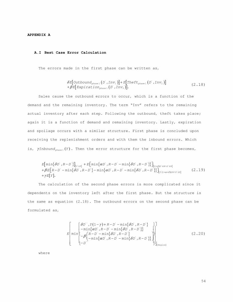
APPENDIX A
A.I Best Case Error Calculation
The errors made in the first phase can be written as,
( )[ ] ( )[ ]( )[ ]
' '1 1 1 2
'1 3
, ,, .
phase phase
phase
E Outbound D Inv E Theft D InvE Expiration D Inv
δβ
++
(2.18)
Sales cause the outbound errors to occur, which is a function of the
demand and the remaining inventory. The term “Inv” refers to the remaining
actual inventory after each step. Following the outbound, theft takes place;
again it is a function of demand and remaining inventory. Lastly, expiration
and spoilage occurs with a similar structure. First phase is concluded upon
receiving the replenishment orders and with them the inbound errors. Which
is, ( )1phaseInbound Yγ . Then the error structure for the first phase becomes,
{ }[ ]{ } { }{ } ( ){ }
{ } { }{ } ( ){ }[ ]
' ' '
' '
' ' ' ' ' '
1' ' ' ' ' ' '
1
min , min , min ,
min , min , min ,
.
D R D R D R
D R D R
E D R D E D R D D R D
E R D D R D D R D D R D
E Y
δ
α δ
δ α δβ δ α δγ
≤ + ≤ ∩ ≤
+ + ≤ ∩ ≤
− + − − − + − − − − − − − +
(2.19)
The calculation of the second phase errors is more complicated since it
dependents on the inventory left after the first phase. But the structure is
the same as equation (2.18). The outbound errors on the second phase can be
formulated as,
( ) { }{ }{ }
{ }{ }{ }
{ }
'' ' ' '
' ' ' '
' ' '
' ' ' '
''
, 1 min ,min , min ,
min min ,min , min ,
Region
D Y R D D R DD R D D R D
E R D D R DD R D D R D
D
δ γ δα δ
δβ α δ
− + − − − − − − − − − − − − − − − −
(2.20)
where
54
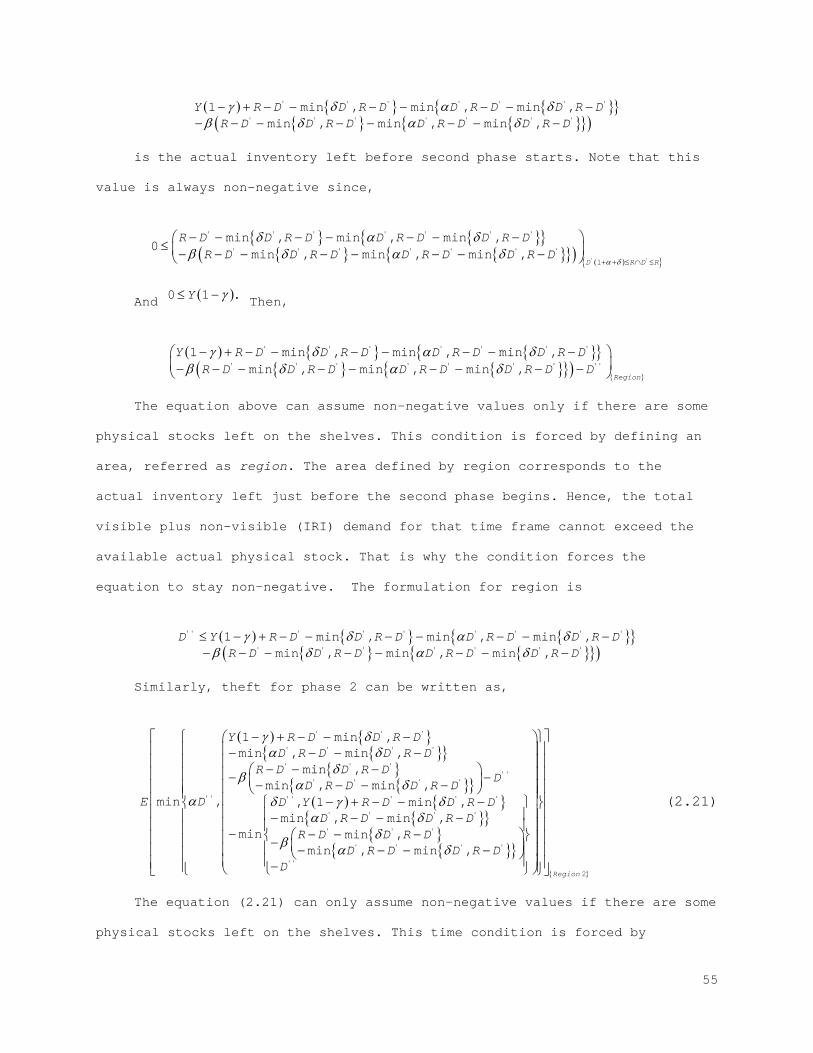
( ) { } { }{ }{ } { }{ }( )
' ' ' ' ' ' '
' ' ' ' ' ' '
1 min , min , min ,min , min , min ,
Y R D D R D D R D D R DR D D R D D R D D R Dγ δ α δ
β δ α δ− + − − − − − − −
− − − − − − − −
is the actual inventory left before second phase starts. Note that this
value is always non-negative since,
{ } { }{ }{ } { }{ }( ) ( ){ }' '
' ' ' ' ' ' '
' ' ' ' ' ' '
1
min , min , min ,0
min , min , min ,D R D R
R D D R D D R D D R DR D D R D D R D D R D
α δ
δ α δβ δ α δ
+ + ≤ ∩ ≤
− − − − − − − ≤ − − − − − − − −
And ( )0 1 .Y γ≤ − Then,
( ) { } { }{ }{ } { }{ }( ) { }
' ' ' ' ' ' '
' ' ' ' ' ' ' ''
1 min , min , min ,min , min , min ,
Region
Y R D D R D D R D D R DR D D R D D R D D R D Dγ δ α δ
β δ α δ− + − − − − − − −
− − − − − − − − −
The equation above can assume non-negative values only if there are some
physical stocks left on the shelves. This condition is forced by defining an
area, referred as region. The area defined by region corresponds to the
actual inventory left just before the second phase begins. Hence, the total
visible plus non-visible (IRI) demand for that time frame cannot exceed the
available actual physical stock. That is why the condition forces the
equation to stay non-negative. The formulation for region is
( ) { } { }{ }{ } { }{ }( )
'' ' ' ' ' ' ' '
' ' ' ' ' ' '
1 min , min , min ,min , min , min ,
D Y R D D R D D R D D R DR D D R D D R D D R D
γ δ α δβ δ α δ
≤ − + − − − − − − −− − − − − − − −
Similarly, theft for phase 2 can be written as,
( ) { }{ }{ }
{ }{ }{ }
( ) { }{ }{ }
{ }
' ' '
' ' ' '
' ' '''
' ' ' '
'' '' ' ' '
' ' ' '
' ' '
' ' '
1 min ,min , min ,
min ,min , min ,
min , , 1 min ,min , min ,
min min ,min , min ,
Y R D D R DD R D D R D
R D D R DD
D R D D R DE D D Y R D D R D
D R D D R DR D D R D
D R D D R
γ δα δ
δβ α δα δ γ δ
α δδβ α δ
− + − − −− − − −
− − − − − − − − − − + − − −
− − − −− − − −− − − − −{ }{ }
{ }
'
''
2Region
DD
−
(2.21)
The equation (2.21) can only assume non-negative values if there are some
physical stocks left on the shelves. This time condition is forced by
55
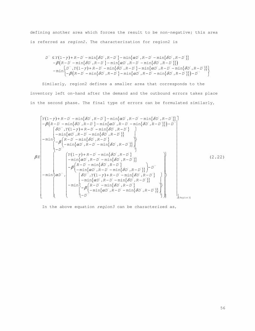
defining another area which forces the result to be non-negative; this area
is referred as region2. The characterization for region2 is
( ) { } { }{ }{ } { }{ }( )
( ) { } { }{ }{ } { }{ }( )
'' ' ' ' ' ' ' '
' ' ' ' ' ' '
'' ' ' ' ' ' ' '
' ' ' ' ' ' ' ''
1 min , min , min ,min , min , min ,
, 1 min , min , min ,min
min , min , min ,
D Y R D D R D D R D D R DR D D R D D R D D R D
D Y R D D R D D R D D R DR D D R D D R D D R D D
γ δ α δβ δ α δ
γ δ α δβ δ α δ
≤ − + − − − − − − −− − − − − − − −
− + − − − − − − − − − − − − − − − − −
Similarly, region2 defines a smaller area that corresponds to the
inventory left on-hand after the demand and the outbound errors takes place
in the second phase. The final type of errors can be formulated similarly,
( ) { } { }{ }{ } { }{ }( )
( ) { }{ }{ }
{ }{ }{ }
' ' ' ' ' ' '
' ' ' ' ' ' ' ''
'' ' ' '
' ' ' '
' ' '
' ' ' '
''
1 min , min , min ,min , min , min ,, 1 min ,
min , min ,min min ,
min , min ,
Y R D D R D D R D D R DR D D R D D R D D R D D
D Y R D D R DD R D D R D
R D D R DD R D D R D
D
E
γ δ α δβ δ α δ
δ γ δα δ
δβ α δ
β
− + − − − − − − −− − − − − − − − −
− + − − −− − − −
− − − − − − − − − −
( ) { }{ }{ }
{ }{ }{ }
( ) { }{ }{ }
{ }
' ' '
' ' ' '
' ' '''
' ' ' '
'' '' ' ' '
' ' ' '
' ' '
'
1 min ,min , min ,
min ,min , min ,
min , , 1 min ,min , min ,
min min ,min ,
Y R D D R DD R D D R D
R D D R DD
D R D D R DD D Y R D D R D
D R D D R DR D D R D
D R
γ δα δ
δβ α δα δ γ δ
α δδβ α
− + − − −− − − −
− − − − − − − − − − − + − − −
− − − −− − − −
− − { }{ }{ }
' ' '
''
3
min ,
Region
D D R DD
δ
− − − −
(2.22)
In the above equation region3 can be characterized as,
56
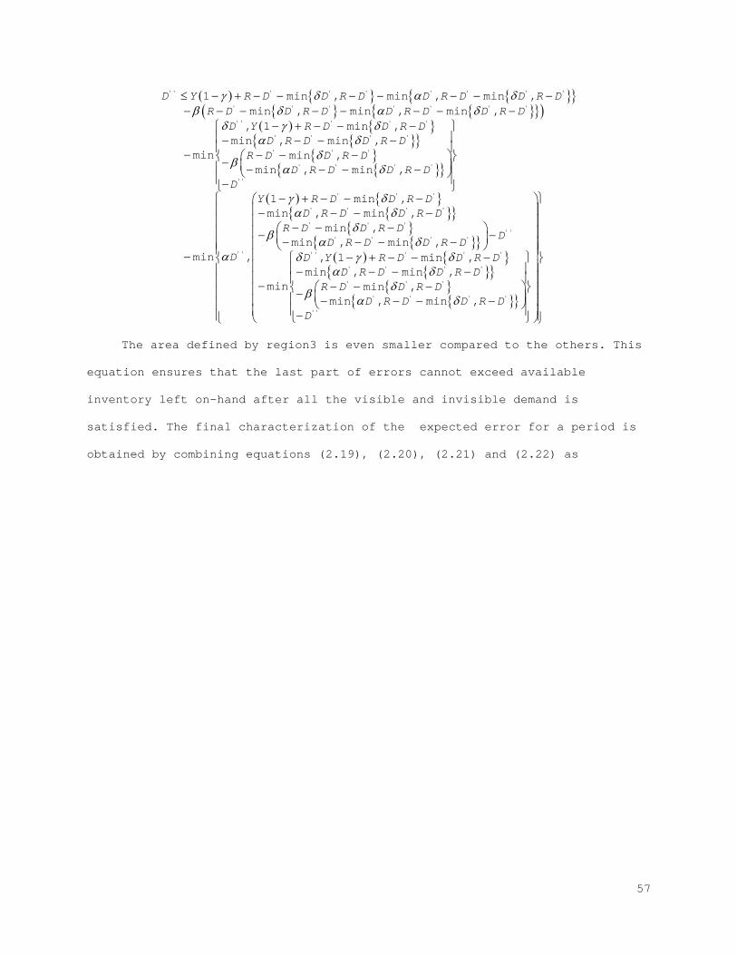
( ) { } { }{ }{ } { }{ }( )
( ) { }{ }{ }
{ }{ }{ }
'' ' ' ' ' ' ' '
' ' ' ' ' ' '
'' ' ' '
' ' ' '
' ' '
' ' ' '
''
1 min , min , min ,min , min , min ,, 1 min ,
min , min ,min min ,
min , min ,
D Y R D D R D D R D D R DR D D R D D R D D R D
D Y R D D R DD R D D R D
R D D R DD R D D R D
D
γ δ α δβ δ α δ
δ γ δα δ
δβ α δ
≤ − + − − − − − − −− − − − − − − −
− + − − −− − − −
− − − − − − − − − −
( ) { }{ }{ }
{ }{ }{ }
( ) { }{ }{ }
{ }
' ' '
' ' ' '
' ' '''
' ' ' '
'' '' ' ' '
' ' ' '
' ' '
'
1 min ,min , min ,
min ,min , min ,
min , , 1 min ,min , min ,
min min ,min ,
Y R D D R DD R D D R D
R D D R DD
D R D D R DD D Y R D D R D
D R D D R DR D D R D
D R D
γ δα δ
δβ α δα δ γ δ
α δδβ α
− + − − −− − − −
− − − − − − − − − − − + − − −
− − − −− − − −
− − − { }{ }' ' '
''min ,D R D
Dδ
− − −
The area defined by region3 is even smaller compared to the others. This
equation ensures that the last part of errors cannot exceed available
inventory left on-hand after all the visible and invisible demand is
satisfied. The final characterization of the expected error for a period is
obtained by combining equations (2.19), (2.20), (2.21) and (2.22) as
57
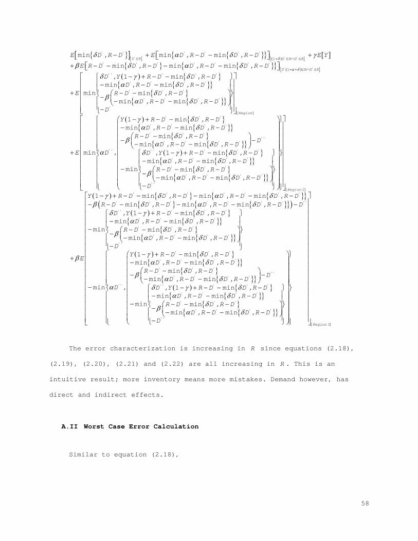
{ }[ ]{ } { }{ } ( ){ } [ ]{ } { }{ } ( ){ }( ) { }
{ }{ }{ }
' ' '
' '
' ' ' ' ' '
1' ' ' ' ' ' '
1'' ' ' '
' ' ' '
' ' '
min , min , min ,
min , min , min ,
, 1 min ,min , min ,
min min ,min
D R D R D R
D R D R
E D R D E D R D D R D E Y
E R D D R D D R D D R D
D Y R D D R DD R D D R D
E R D D R D
δ
α δ
δ α δ γβ δ α δ
δ γ δα δ
δβ α
≤ + ≤ ∩ ≤
+ + ≤ ∩ ≤
− + − − − + + − − − − − − −
− + − − −− − − −
+ − − −− − { }{ }{ }
( ) { }{ }{ }
{ }{ }{ }
( ) { }
' ' ' '
'
' ' '
' ' ' '
' ' '''
' ' ' '
'' '' ' ' '
, min ,
1 min ,min , min ,
min ,min , min ,
min , , 1 min ,
min
Region
D R D D R DD
Y R D D R DD R D D R D
R D D R DD
D R D D R DE D D Y R D D R D
δ
γ δα δ
δβ α δα δ γ δ
− − − − − + − − −
− − − −− − − − − − − − −
+ − + − − −−
−{ }{ }
{ }{ }{ }
{ }
( ) { }
' ' ' '
' ' '
' ' ' '
''
2' ' '
min , min ,min ,
min , min ,
1 min , minRegion
D R D D R DR D D R D
D R D D R DD
Y R D D R D D
E
α δδβ α δ
γ δ α
β
− − − − − − − − − − − −
− + − − − −
+
{ }{ }{ } { }{ }( )
( ) { }{ }{ }
{ }{ }{ }
( )
' ' ' '
' ' ' ' ' ' ' ''
'' ' ' '
' ' ' '
' ' '
' ' ' '
''
''
, min ,min , min , min ,, 1 min ,
min , min ,min min ,
min , min ,
1
min ,
R D D R DR D D R D D R D D R D D
D Y R D D R DD R D D R D
R D D R DD R D D R D
DY R
D
δβ δ α δ
δ γ δα δ
δβ α δ
γ
α
− − −− − − − − − − − −
− + − − − − − − − − − − − − − − − − −
− + −
−
{ }{ }{ }
{ }{ }{ }
( ) { }{ }{ }
{ }{ }{ }
' ' '
' ' ' '
' ' '''
' ' ' '
'' ' ' '
' ' ' '
' ' '
' ' ' '
''
min ,min , min ,
min ,min , min ,
, 1 min ,min , min ,
min min ,min , min ,
D D R DD R D D R D
R D D R DD
D R D D R DD Y R D D R D
D R D D R DR D D R D
D R D D R DD
δα δ
δβ α δδ γ δ
α δδβ α δ
− −− − − −
− − − − − − − − − − + − − −
− − − −− − − − − − − − − −
{ }3Region
The error characterization is increasing in R since equations (2.18),
(2.19), (2.20), (2.21) and (2.22) are all increasing in R . This is an
intuitive result; more inventory means more mistakes. Demand however, has
direct and indirect effects.
A.II Worst Case Error Calculation
Similar to equation (2.18),
58
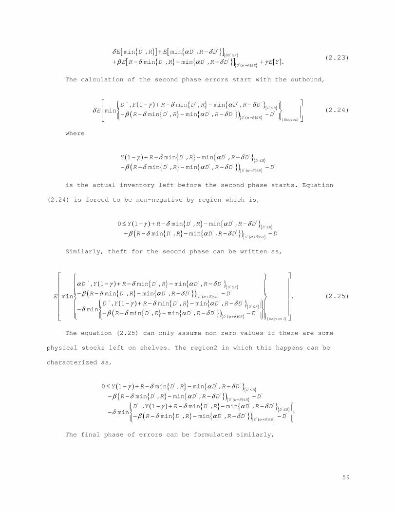
{ }[ ] { }[ ]{ }
{ } { }[ ] ( ){ } [ ]'
'
' ' '
' ' '
min , min ,
min , min , .D R
D R
E D R E D R D
E R D R D R D E Yδ
α δ
δ α δβ δ α δ γ
≤
+ ≤
+ −
+ − − − + (2.23)
The calculation of the second phase errors start with the outbound,
( ) { } { }{ }
{ } { }( ) ( ){ } { }
'
'
'' ' ' '
' ' ' '
, 1 min , min ,min
min , min ,D R
D R Region
D Y R D R D R DE
R D R D R D Dα δ
γ δ α δδ β δ α δ
≤
+ ≤
− + − − − − − − − − (2.24)
where
( ) { } { }{ }{ } { }( ) ( ){ }
'
'
' ' '
' ' ' '
1 min , min ,
min , min ,D R
D R
Y R D R D R D
R D R D R D Dα δ
γ δ α δβ δ α δ
≤
+ ≤
− + − − −− − − − −
is the actual inventory left before the second phase starts. Equation
(2.24) is forced to be non-negative by region which is,
( ) { } { }{ }{ } { }( ) ( ){ }
'
'
' ' '
' ' ' '
0 1 min , min ,
min , min ,D R
D R
Y R D R D R D
R D R D R D Dα δ
γ δ α δβ δ α δ
≤
+ ≤
≤ − + − − −− − − − −
Similarly, theft for the second phase can be written as,
( ) { } { }{ }{ } { }( ) ( ){ }( ) { } { }{ }
{ } { }( ) ( ){ } { }
'
'
'
'
'' ' ' '
' ' ' '
'' ' ' '
' ' ' '
2
, 1 min , min ,
min , min ,min, 1 min , min ,
minmin , min ,
D R
D R
D R
D RRegion
D Y R D R D R D
R D R D R D DED Y R D R D R D
R D R D R D D
α δ
α δ
α γ δ α δβ δ α δ
γ δ α δδ β δ α δ
≤
+ ≤
≤
+ ≤
− + − − − − − − − − − + − − − − − − − − −
.
(2.25)
The equation (2.25) can only assume non-zero values if there are some
physical stocks left on shelves. The region2 in which this happens can be
characterized as,
( ) { } { }{ }{ } { }( ) ( ){ }( ) { } { }{ }
{ } { }( ) ( ){ }
'
'
'
'
' ' '
' ' ' '
'' ' ' '
' ' ' '
0 1 min , min ,
min , min ,
, 1 min , min ,min
min , min ,
D R
D R
D R
D R
Y R D R D R D
R D R D R D D
D Y R D R D R D
R D R D R D D
α δ
α δ
γ δ α δβ δ α δ
γ δ α δδ β δ α δ
≤
+ ≤
≤
+ ≤
≤ − + − − −− − − − −
− + − − − − − − − − −
The final phase of errors can be formulated similarly,
59
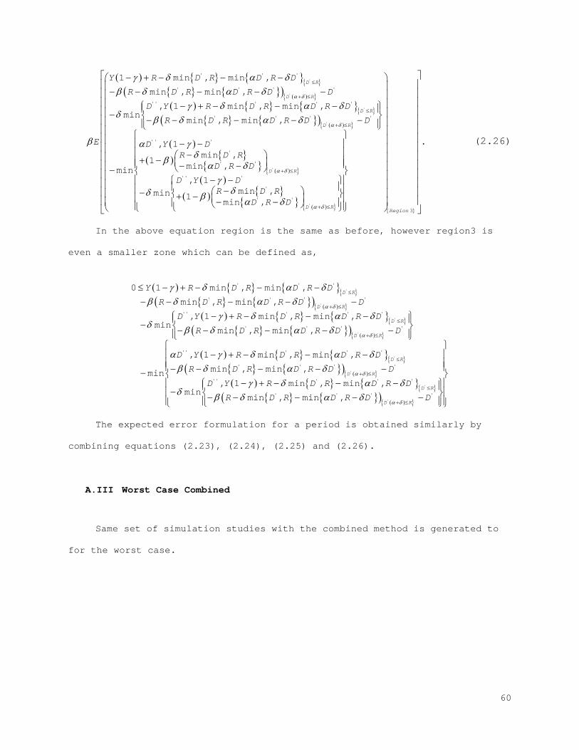
( ) { } { }{ }{ } { }( ) ( ){ }( ) { } { }{ }
{ } { }( ) ( ){ }
( )
( ) { }{ }
'
'
'
'
' ' '
' ' ' '
'' ' ' '
' ' ' '
'' '
'
' '
1 min , min ,
min , min ,
, 1 min , min ,min
min , min ,
, 1min ,
1min ,min
D R
D R
D R
D R
Y R D R D R D
R D R D R D D
D Y R D R D R D
R D R D R D D
E D Y DR D R
D R D
α δ
α δ
γ δ α δβ δ α δ
γ δ α δδ β δ α δ
β α γδβ α δ
≤
+ ≤
≤
+ ≤
− + − − −− − − − −
− + − − − − − − − − −
− −−+ − − −− ( ){ }
( )
( ) { }{ } ( ){ } { }
'
'
'' '
'
' '
3
.
, 1min ,min 1
min ,
D R
D RRegion
D Y DR D R
D R D
α δ
α δ
γδδ β α δ
+ ≤
+ ≤
− − − − + − − −
(2.26)
In the above equation region is the same as before, however region3 is
even a smaller zone which can be defined as,
( ) { } { }{ }{ } { }( ) ( ){ }( ) { } { }{ }
{ } { }( ) ( ){ }
( ) { } { }{ }
'
'
'
'
'
' ' '
' ' ' '
'' ' ' '
' ' ' '
'' ' ' '
0 1 min , min ,
min , min ,
, 1 min , min ,min
min , min ,
, 1 min , min ,
min
D R
D R
D R
D R
D R
Y R D R D R D
R D R D R D D
D Y R D R D R D
R D R D R D D
D Y R D R D R D
R
α δ
α δ
γ δ α δβ δ α δ
γ δ α δδ β δ α δ
α γ δ α δβ
≤
+ ≤
≤
+ ≤
≤
≤ − + − − −− − − − −
− + − − − − − − − − −
− + − − −− −− { } { }( ) ( ){ }
( ) { } { }{ }{ } { }( ) ( ){ }
'
'
'
' ' ' '
'' ' ' '
' ' ' '
min , min ,
, 1 min , min ,min
min , min ,
D R
D R
D R
D R D R D D
D Y R D R D R D
R D R D R D D
α δ
α δ
δ α δγ δ α δ
δ β δ α δ
+ ≤
≤
+ ≤
− − −
− + − − − − − − − − −
The expected error formulation for a period is obtained similarly by
combining equations (2.23), (2.24), (2.25) and (2.26).
A.III Worst Case Combined
Same set of simulation studies with the combined method is generated to
for the worst case.
60
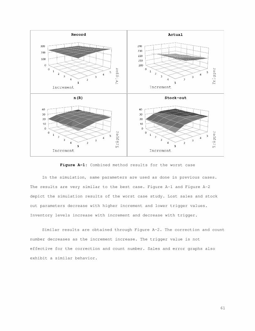
Figure A-1: Combined method results for the worst case
In the simulation, same parameters are used as done in previous cases.
The results are very similar to the best case. Figure A-1 and Figure A-2
depict the simulation results of the worst case study. Lost sales and stock
out parameters decrease with higher increment and lower trigger values.
Inventory levels increase with increment and decrease with trigger.
Similar results are obtained through Figure A-2. The correction and count
number decreases as the increment increase. The trigger value is not
effective for the correction and count number. Sales and error graphs also
exhibit a similar behavior.
61
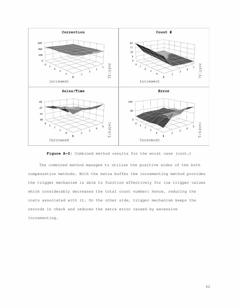
Figure A-2: Combined method results for the worst case (cont.)
The combined method managed to utilize the positive sides of the both
compensation methods. With the extra buffer the incrementing method provides
the trigger mechanism is able to function effectively for low trigger values
which considerably decreases the total count number; hence, reducing the
costs associated with it. On the other side, trigger mechanism keeps the
records in check and reduces the extra error caused by excessive
incrementing.
62
CHAPTER 3 IRI ANALYSIS IN ONLINE RETAILING WITH LEAD TIME AND SUPPLY
UNCERTAINTY
With the advancement of the Internet, online retailing becomes an
important channel for retails. According to Mangalindan (2005), 5.5% of all
retail sales (excluding travel) are done online in 2004. This potential is
recognized by many organizations as demonstrated in Tsay and Agrawal (2004).
The major difference of the online retail environment is that customers do
not have access to the goods during purchase. This fact greatly enhances the
importance of inventory records since the amount of sales is highly dependent
on the accuracy of the records.
IRI is a well-known problem for both the online and the offline retail
environment. In this context IRI is regarded as the mismatch between the
inventory records and the actual physical stock. In large scale retailing,
the inventory records are likely to be incorrect, and ignoring this fact
often leads to failed re-procurement cycles and quantities. Inventory models
with IRI are commonly studied in the offline retail environment, but there
are limited studies for the online retails.
The online and the offline retail models are similar on many aspects. But
one crucial difference is: In the online retails, customers make their
purchasing decisions based on inventory records where as in the offline
retails customer are allowed to pick the product from shelves directly. This
difference has various implications on the IRI behavior. Our aim in this
chapter is to develop a model to identify the effects of customers’
interaction with physical stock and understand the behavior IRI in the online
retailing environment.
63
This chapter also classifies IRI in three groups: inbound, shelving and
outbound errors. While the customer interaction has little effect on inbound
and outbound types of IRI, it is quite influential on shelving errors. In
fact it is commonly known that customer interaction in the supply chain is a
major source of shelving errors (Rekik et al., 2009). The online model lacks
this interaction; however, a substantial amount of shelving errors can still
take place even without the presence of customers. According to Center for
Retail Research (2005) the average rate for shelving errors in UK is 1.4%
percent of sales, which is one of the highest in Europe. The study also
identifies that 14.4% of shelving errors can be attributed to internal
errors, such as processing errors, accounting mistakes and pricing
discrepancies.
In this chapter, we investigate the online retail models where the
customers are not allowed to directly interact with products; instead they
make their purchasing decision based solely on the inventory records (Grewal
et al., 2004). Furthermore, we characterize the structure of IRI when it is
influenced by random supply, random demand and random lead time in the online
setting where the inventory records are reviewed continuously.
3.1 Model
IRI is influenced by many factors such as demand, supply and lead time
apart from the direct causes (shrinkage, transaction and misplacement
errors). The difficulty in modeling IRI generally lies in the fact that the
relationship is not one sided, IRI affects all of these factors back. In
addition, the online retail environment has three main distinctive features.
First, the customers do not have access to the inventory; therefore, the
demand is satisfied based on the inventory records and not by the actual
64
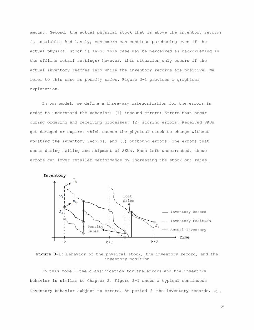
amount. Second, the actual physical stock that is above the inventory records
is unsalable. And lastly, customers can continue purchasing even if the
actual physical stock is zero. This case may be perceived as backordering in
the offline retail settings; however, this situation only occurs if the
actual inventory reaches zero while the inventory records are positive. We
refer to this case as penalty sales. Figure 3-1 provides a graphical
explanation.
In our model, we define a three-way categorization for the errors in
order to understand the behavior: (1) inbound errors: Errors that occur
during ordering and receiving processes; (2) storing errors: Received SKUs
get damaged or expire, which causes the physical stock to change without
updating the inventory records; and (3) outbound errors: The errors that
occur during selling and shipment of SKUs. When left uncorrected, these
errors can lower retailer performance by increasing the stock-out rates.
Figure 3-1: Behavior of the physical stock, the inventory record, and the inventory position
In this model, the classification for the errors and the inventory
behavior is similar to Chapter 2. Figure 3-1 shows a typical continuous
inventory behavior subject to errors. At period k the inventory records, kt
x ,
65
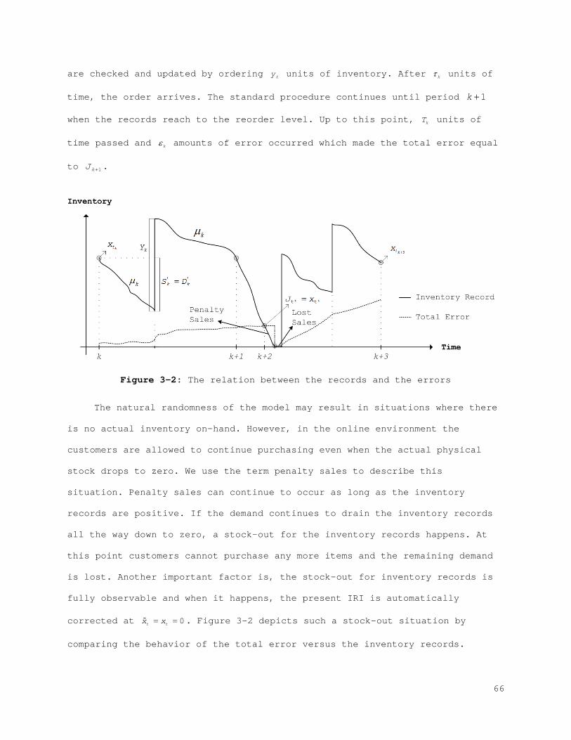
are checked and updated by ordering ky units of inventory. After kτ units of
time, the order arrives. The standard procedure continues until period 1k +
when the records reach to the reorder level. Up to this point, kT units of
time passed and kε amounts of error occurred which made the total error equal
to 1kJ + .
Figure 3-2: The relation between the records and the errors
The natural randomness of the model may result in situations where there
is no actual inventory on-hand. However, in the online environment the
customers are allowed to continue purchasing even when the actual physical
stock drops to zero. We use the term penalty sales to describe this
situation. Penalty sales can continue to occur as long as the inventory
records are positive. If the demand continues to drain the inventory records
all the way down to zero, a stock-out for the inventory records happens. At
this point customers cannot purchase any more items and the remaining demand
is lost. Another important factor is, the stock-out for inventory records is
fully observable and when it happens, the present IRI is automatically
corrected at 0t tx x= = . Figure 3-2 depicts such a stock-out situation by
comparing the behavior of the total error versus the inventory records.
66
Let ktx denote the amount of actual inventory and
ktx denote the
inventory record at time kt in period k . Also let, ky be the order quantity
and kD be the total demand in period k . Suppose that demand has a known
distribution function ( ) { }DF z P D z= ≤ with a density ( )Df z . Furthermore, let kS
be the amount of sales and kε be the discrepancy between the actual and the
recorded inventory during period k . When there is, no lead time and no random
supply, inventory progression can be formulated as
1k k kt k t t k k
k K
x x x y Sε−
∈
+ = = + −∑ , (3.1)
where { }min ,kk k tD xS = is the amount of sales for 0 k kS x≤ ≤ and kε is the mismatch
at period k . Furthermore, we introduce the supply uncertainty using the same
setup presented in Section 2.1 as { }[ ]min , kE U K y , where K represents the random
capacity and U denotes the random yield of the supplier (Erdem & Ozekici,
2002; Henig & Gerchak, 1990). Then, equation (3.1) can be rewritten as
[ ] { }[ ] [ ]1
0
min ,k k k k k
k
t t k ii
E U K yE x EEx S ε−
=
= − −
+ ∑ . (3.2)
3.1.1 Error Modeling
The total errors incurred until period k is denoted by
0
k
ii
E ε=
∑ .
Note that we consider errors as previously classified. In this
classification the shelving errors are only caused by expiration or spoilage
( ekε ) since customers are not allowed to physically interact with the
products. Yan et al. (2011) provide a general characterization for expired
and damaged items in inventory models. We modify their model to fit the
67
online retail environment as, { }max ,0k
ek t kx Sβε = − where [ ]0,1β ∈ is the rate of
expiration/spoilage. Expiration errors occur from the unsold inventory at the
end of each period; which can be simplified as, ( )k
ek t kx Dε β= − . Moreover, r
kε
denotes the inbound errors which are related to the order quantity; whereas,
the outbound errors, skε , are dependent on the number of units sold. Rosetti
et al. (2010) provide detailed insights about the structure of the
transaction errors. In this setting rk kyε γ= and s
k kSε δ= where
'
'1,R S
Dγ − ∈
and
( )
( )21
1,1
β β βδ
β
+ − ∈ − − .
The general formulation derived in Section 2.1.2 is modified according to
the online retail framework as
[ ] { }[ ] [ ]
{ }( )[ ]
{ }
{ }[ ] [ ]{ }
1
0
0 0
min ,
min , .
ixk k xi i
xi
k k D
i
D
D
k
t t k k k k t ii
k k
i i ii
ii
E x x E U K y E D E x D
E U K y E D
β
γ δ
≤ ≤
≤
−=
= =
= + − − −
+ +
∑
∑ ∑
(3.3)
Then, the inventory formulation can be modified accordingly to obtain the
error function, [ ] [ ]k k kt t tE J E x x= − . Using the inventory relation in equation
(3.1), equation (3.3) can be rewritten as
[ ] [ ]{ }
[ ]{ }
{ }[ ]0 0 0
min ,i xi ixi i
k k DD
k k k
t t t i i i ii i i
iE x x E x D E D E U K yβ δ γ≤≤
= = =
= − − + +− ∑ ∑ ∑ . (3.4)
Therefore, the total expected error at period k when the current period is i
can be modeled as,
68
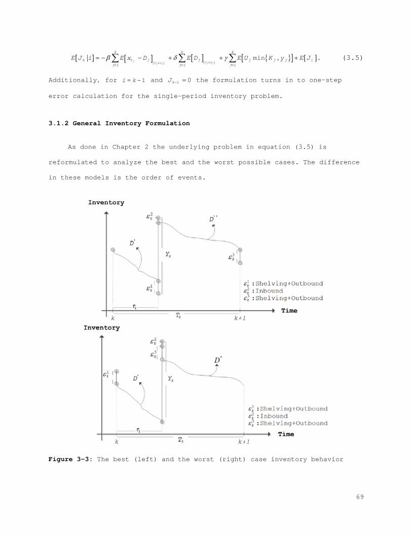
[ ] [ ]{ }
[ ]{ }
{ }[ ] [ ]min ,j xj jxj DjD
k k k
k t j jj i j i
j ij
j ji
E J i E x D E D E U K y E Jβ δ γ≤≤= = =
= − − + + +∑ ∑ ∑ . (3.5)
Additionally, for 1i k= − and 1 0kJ − = the formulation turns in to one-step
error calculation for the single-period inventory problem.
3.1.2 General Inventory Formulation
As done in Chapter 2 the underlying problem in equation (3.5) is
reformulated to analyze the best and the worst possible cases. The difference
in these models is the order of events.
Figure 3-3: The best (left) and the worst (right) case inventory behavior
69
Figure 3-3 shows the order of events for each model. Each period is
divided into two phases; the first phase contains the lead time demand and
the second phase contains the demand for the rest of the period.
Replenishment time determines the end of the first phase.
In the best case framework the demand is fulfilled first and then errors
occur. Since sold items are outside of the feasible space for errors, this
case maximizes the demand fill rate and minimizes the IRI. In the worst case,
the errors occur first and then the demand is fulfilled; thus, minimizing the
fill rate. In reality, the inventory behaves somewhere between the best and
the worst case situations; hence, the two characterizations provide a lower
and an upper bound. In this case 1kε denotes the outbound and storing errors
during lead time, 2kε denotes the inbound errors, and 3
kε denotes the outbound
and the storing errors during the remainder of period k .
i. Best Case
The errors done in the first phase for the best case are,
{ }[ ] { }[ ] [ ]' ' ' ' 'min , min , .E D R S E R S D R S E Yδ β δ γ− + − − − + (3.6)
The calculation of the second phase errors depends on the inventory left
which is
[ ]( ) [ ] { }[ ] { }[ ]' ' ' ' ' '1 min , min ,E Y R E S E D R S E R S D R Sγ δ β δ− + − − − − − − − (3.7)
Note that equation (3.7) is always non-negative and can assume positive
values only if there are some physical stocks left on shelves. This can
easily be proven by choosing the highest 1β = , which corresponds to the
extreme situation where all the inventory is lost at the end of the phase. In
that case, equation (3.7) becomes [ ]( )1E Y γ− which is always non-negative.
70
The second phase in the best case starts off with the demand, which can
be written as
[ ]( ) [ ] { }[ ] { }[ ] [ ]' ' ' ' ' ' ''1 min , min ,E Y R E S E D R S E R S D R S E Dγ δ β δ− + − − − − − − − − . (3.8)
Equation (3.8) represents the available inventory before the next source of
error occurs. Note that, equation (3.8) is always positive as long as
( ) '1Y Dγ− ≤ . This provides a lower bound for γ . The outbound errors on the
second phase can be formulated as
( ) { } { }( ){ }'' ' '' ' ' ' ' 'min , 1 min , min ,E D Y R S D D R S R S D R Sδ γ δ β δ − + − − − − − − − − . (3.9)
Finally the storing errors can be formulated similarly,
( ) { } { }( )( ) { } { }( ){ }' '' ' ' ' ' '
'' ' '' ' ' ' ' '
1 min , min ,min , 1 min , min ,
Y R S D D R S R S D R SE
D Y R S D D R S R S D R Sγ δ β δβ δ γ δ β δ
− + − − − − − − − −− − + − − − − − − − −
(3.10)
The final characterization of the expected error for a period is obtained by
combining equations (3.6), (3.9) and (3.10) as
[ ] { }[ ] { }[ ] [ ]( ) { }
{ }( )( ) ( ) { }( )
( ) ( ) { }( ){ }
' ' ' ' '
'' ' '' ' '
' ' '
'' ' ' '
'' ' ' '
min , min ,, 1 min ,
minmin ,
1 1 min ,.
min , 1 1 min ,
E J E D R S E R S D R S E YD Y R S D D R S
ER S D R S
Y D R S D R SE
D Y R S D R S
δ β δ γδ γ δβ δγ β δβ δ γ β δ
= − + − − − +− + − − − − + − − − −
− − + − − − − + − − + − − − −
(3.11)
Reorder level dependency
[ ]E J is increasing in R since the partial derivative with respect to R
is positive. This can be shown by separating equation (3.11) into three
terms. For practicality, we let [ ]iE J denote the line 1,2,3i = for equations
(3.6), (3.9) and (3.10) respectively, so that [ ] [ ] [ ] [ ]1 2 3E J E J E J E J= + + . Then,
the derivation of [ ]1E J is,
[ ]{ }( ){ } { } { }( ){ }( )' ' '' ' ' '
1
1 1 1 1 1 1D R D R D RR S D R S D
E JR δ δ
β≥ ≥ ≥− ≤ − ≤
∂= − + − − −
∂.
71
The derivative is non-negative since { }( ){ }' ' '1 1 0D R R S Dδ≥ − ≤− ≥ and [ ]0,1β ∈ . The
derivative of [ ]2E J is,
[ ]( ) ( ) { }( ){ }
( ) { } { }( ){ }( ) ( ) ( ) { }( ){ }' ' ' ' '' '' ' ' '
2'' '' ' ' '
1 1 min ,
min , 1 1 min ,
1 1 1 1 1 .D R D R R S D D Y D R S D R S
E JE D Y D R S D R S
R Rδ δ γ β δ
δ γ β δβ ≥ ≥ − ≤ ≥ − − + − − − −
∂ ∂= − − + − − − − ∂ ∂= − − − −
Since [ ]0,1β ∈ and { }'1 1 0D R≥− ≥ , the above equation is again always non-negative.
The final part can be written as,
[ ] ( ) ( ) { }( )( ) ( ) { }( ){ }
( ) { } { }( ){ }( )( ) { } { }( ){ }( ) ( ) ( ) { }( ){ }
' ' ' '
' ' ' ' '' ' ' '
'' ' ' '3
'' ' ' '
1 1 min ,
1 1 min ,min , 1 1 min ,
1 1 1 1 11 1 1 1 1
D R D R R S D
D R D R R S D D Y R S D R S
Y D R S D R SE JE
D Y R S D R SR R
δ
δ δ γ β δ
γ β δβ δ γ β δβ
β β≥ ≥ − ≤
≥ ≥ − ≤ ≥ − + − − − −
− − + − − − −∂ ∂ = − − + − − − −∂ ∂
− − − − = − − − − −
Hence, the summation of [ ] [ ] [ ]1 2 3E J E J E J+ + is increasing in R when 'R D≥
or it is zero.
Lead time demand dependency
The function behavior with the first phase demand can be found by taking
the derivative with respect to 'D . Let [ ] [ ] [ ] [ ]1 2 3E J E J E J E J= + + then,
[ ]{ } { } { } { }( ){ } { }( )( )
' ' ' ' ' ' ' '
' ' ' '
1
'
' '
' '
1 1
1 1
.1
R S D R D D R S D R D D
R S D R D D
E J
D
R S DR S D
δ δ δ δ
δ δ
δ β β δδ β βδ δβ β δ
δ
− ≥ − < − ≥ − <
− ≥ − <
∂= − − − −
∂= − − −
− − − ≥= − − <
[ ]1E J behaves differently based on δ and β . When δ is big enough [ ]1E J
is decreasing with 'D , but when δ is small it depends on both β and δ . The
derivative of [ ]2E J with respect to 'D is,
72
[ ][ ]{ }
{ }
[ ]
[ ]{ }'
'' 1
2'' ' '' 1
'
1
'
min ,
1 .D RD Y R D E J
E JE D Y R S D E J
DE J
D δ
δ
≤≥ + − −
∂= + − − − ∂
∂ = − − ∂
[ ]2E J is also decreasing for big enough δ , otherwise it also depends on both
δ and β through [ ]1E J . Finally, the derivative of [ ]3E J is,
[ ][ ] [ ]( )
{ }
[ ] [ ]'
3' '' 1 2
' '
1 2
' '1 .D R
E JY R S D E J E J
D DE J E J
D D
β
β ≤
∂ ∂= + − − − −
∂ ∂∂ ∂ = − − −
∂ ∂
Once again the behavior is dependent on δ and β .
ii. Worst Case
In the worst case, it is assumed that IRI takes place prior to demand
fulfillment. Similar to the best case, the inbound errors during the first
phase can be obtained as,
[ ] [ ] [ ]' ' .E S E R S E Yδ β δ γ+ − + (3.12)
The calculation of the second phase errors start with the outbound errors,
( ) ( ){ }'' ' ' 'min , 1E D Y R S S R Sδ γ δ β δ− + − − − − (3.13)
where ( ) ( )' ' '1Y R S S R Sγ δ β δ− + − − − − is the actual remaining inventory on the
shelves. When 1β = , the on-hand inventory becomes ( ) '1Y Sγ− − . Recall that, due
to the nature of the online retail sales, customers can continue purchasing
even when the actual physicals stock is zero. Hence, ( ) '1Y Sγ− − can be
negative, but ( )1Y γ− is always positive. The final phase of errors can be
formulated similarly,
( ) ( ) ( ) ( ){ }( )[ ]' ' '' ' ' '1 min , 1 .Y R S S R S D Y R S S R SE γ δ β δ δ γ δ β δβ − + − − − − − − + − − − − (3.14)
73
Also note that, equation (3.14) is always positive when ( ) '1Y Sγ− ≥ . The
expected error formulation for a period is obtained similarly by combining
equations (3.12), (3.13) and (3.14) as,
[ ] [ ] [ ] ( ) ( ){ }( ) ( ) ( ) ( ){ }( )[ ]' ' ' '' ' ' '
' ' '' ' ' '
1 min , 1 .min , 1
Y R S S R S D Y R S S R SE S E R S E Y E D Y R S S R SE γ δ β δ δ γ δ β δ
δ β δ γ δ γ δ β δβ − + − − − − − − + − − − −
+ − + + − + − − − − +
(3.15)
Reorder level dependency
[ ]E J in the worst case setup is again increasing in R since the partial
derivative with respect to R is positive. This can be shown as
[ ]( ) ( ) ( ){ } ( ) ( ) ( ){ }( )( ) ( )( ) ( ) ( ){ }
" ' ' ' " ' ' '
" ' ' '
1 1
1
1 1 1
1 1 1 .D Y R D R D D D Y R D R D D
D Y R D R D D
E JR γ δ β δ γ δ β δ
γ δ β δ
β δ β β β δ ββ β β δ β β
≤ − + − − − − ≤ − + − − − −
≤ − + − − − −
∂= + − + − − −
∂= + − + − −
This equation is non-negative, as long as,
( )
( )21
1
β β βδ
β
+ −≥ −
−. (3.16)
Equation (3.16) is decreasing in terms of β since the derivative with
respect to β is negative. Thus, the lower bound for δ decreases as β
increases.
Lead time demand dependency
The function behavior with the first phase demand can be found by taking
the derivative with respect to 'D . In other words,
[ ]( ) ( ) ( ){ }
( )( ) ( ) ( ){ }( ) ( ) ( ){ } ( ) ( )
'' ' ' '
'' ' ' '
'' ' ' '
1'
1
1
1
1 11 1 .
D Y R D R D D
D Y R D R D D
D Y R D R D D
E J
D γ δ β δ
γ δ β δ
γ δ β δ
δ βδ δ βδ δ
β δ βδ δ βδ δβδ δ δ β βδ δ β
≥ − + − − − −
≥ − + − − − −
≥ − + − − − −
∂= − + − −
∂+ − + − − − −= − − + − + −
Just like the best case this function’s behavior depends on the relation
between δ and β .
74
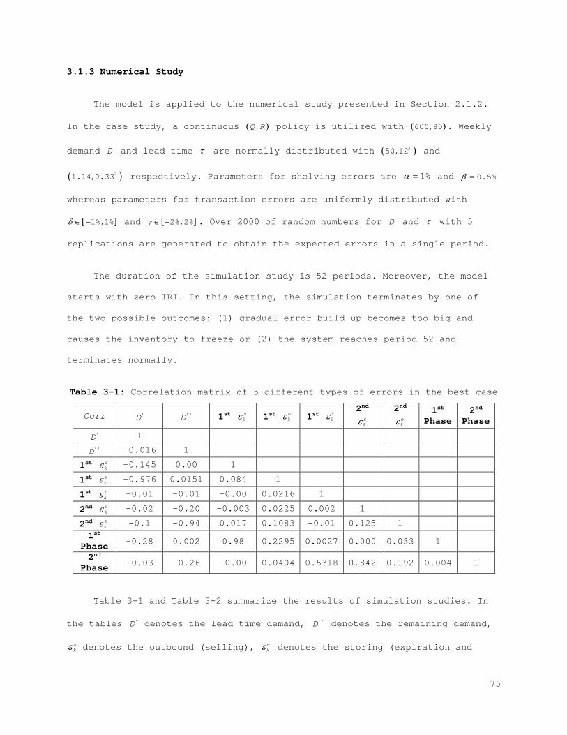
3.1.3 Numerical Study
The model is applied to the numerical study presented in Section 2.1.2.
In the case study, a continuous ( ),Q R policy is utilized with ( )600,80 . Weekly
demand D and lead time τ are normally distributed with ( )250,12 and
( )21.14,0.33 respectively. Parameters for shelving errors are 1%α = and 0.5%β =
whereas parameters for transaction errors are uniformly distributed with
[ ]1%,1%δ ∈ − and [ ]2%,2%γ ∈ − . Over 2000 of random numbers for D and τ with 5
replications are generated to obtain the expected errors in a single period.
The duration of the simulation study is 52 periods. Moreover, the model
starts with zero IRI. In this setting, the simulation terminates by one of
the two possible outcomes: (1) gradual error build up becomes too big and
causes the inventory to freeze or (2) the system reaches period 52 and
terminates normally.
Table 3-1: Correlation matrix of 5 different types of errors in the best case
Corr 'D ''D 1st skε 1st e
kε 1st rkε
2nd skε
2nd ekε
1st Phase
2nd Phase
'D 1 ''D -0.016 1
1st skε -0.145 0.00 1
1st ekε -0.976 0.0151 0.084 1
1st rkε -0.01 -0.01 -0.00 0.0216 1
2nd skε -0.02 -0.20 -0.003 0.0225 0.002 1
2nd ekε -0.1 -0.94 0.017 0.1083 -0.01 0.125 1
1st Phase -0.28 0.002 0.98 0.2295 0.0027 0.000 0.033 1
2nd Phase -0.03 -0.26 -0.00 0.0404 0.5318 0.842 0.192 0.004 1
Table 3-1 and Table 3-2 summarize the results of simulation studies. In
the tables 'D denotes the lead time demand, ''D denotes the remaining demand,
skε denotes the outbound (selling), e
kε denotes the storing (expiration and
75
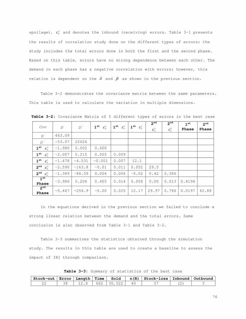
spoilage), rkε and denotes the inbound (receiving) errors. Table 3-1 presents
the results of correlation study done on the different types of errors; the
study includes the total errors done in both the first and the second phase.
Based on this table, errors have no strong dependence between each other. The
demand in each phase has a negative correlation with errors; however, this
relation is dependent on the δ and β as shown in the previous section.
Table 3-2 demonstrates the covariance matrix between the same parameters.
This table is used to calculate the variation in multiple dimensions.
Table 3-2: Covariance Matrix of 5 different types of errors in the best case
Cov 'D ''D 1st skε 1st e
kε 1st rkε
2nd skε
2nd ekε
1st Phase
2nd Phase
'D 463.09 ''D -53.07 22626
1st skε -1.980 0.002 0.400
1st ekε -2.007 0.215 0.005 0.009
1st rkε -1.478 -4.531 -0.001 0.007 12.1
2nd skε -2.590 -163.8 -0.01 0.011 0.052 29.5
2nd ekε -1.389 -88.59 0.006 0.006 -0.02 0.42 0.386
1st Phase -3.986 0.206 0.405 0.014 0.006 0.00 0.013 0.4194
2nd Phase -5.467 -256.9 -0.00 0.025 12.17 29.97 0.786 0.0197 42.88
In the equations derived in the previous section we failed to conclude a
strong linear relation between the demand and the total errors. Same
conclusion is also observed from Table 3-1 and Table 3-2.
Table 3-3 summarizes the statistics obtained through the simulation
study. The results in this table are used to create a baseline to assess the
impact of IRI through comparison.
Table 3-3: Summary of statistics of the best case
Stock-out Error Length Time Sold n(R) Stock-loss Inbound Outbound 22 38 12.8 662 30,522 40 37 (2) 3
76
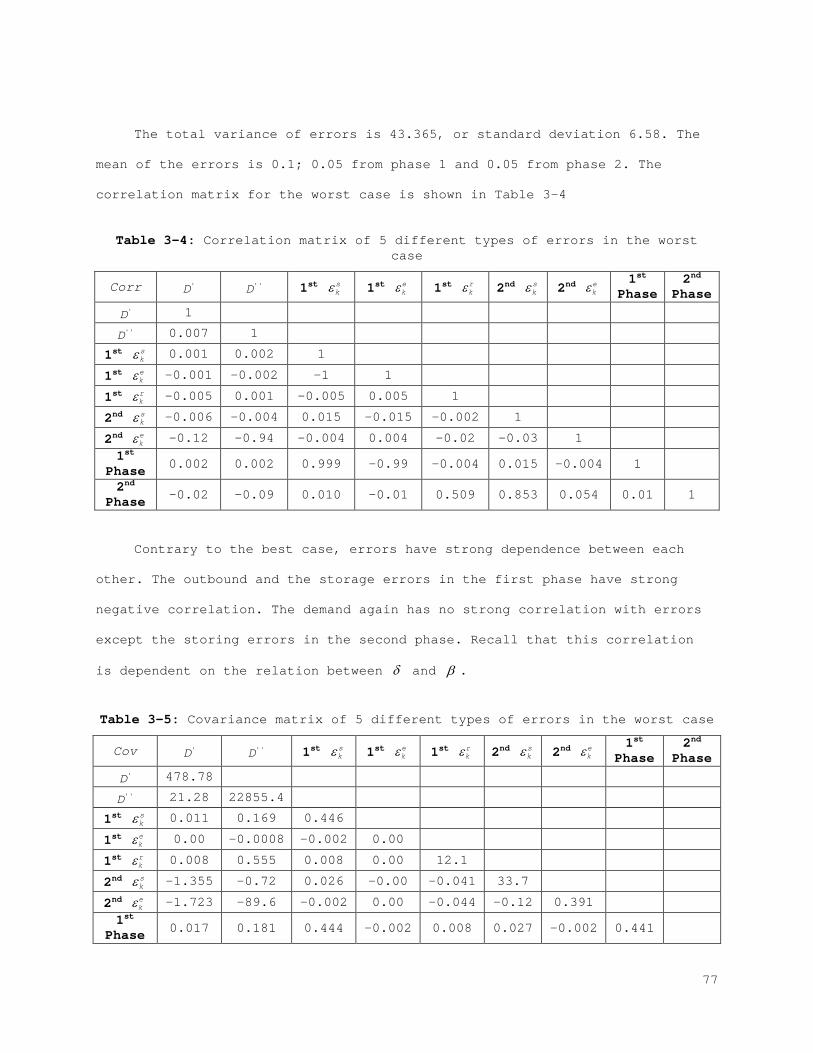
The total variance of errors is 43.365, or standard deviation 6.58. The
mean of the errors is 0.1; 0.05 from phase 1 and 0.05 from phase 2. The
correlation matrix for the worst case is shown in Table 3-4
Table 3-4: Correlation matrix of 5 different types of errors in the worst case
Corr 'D ''D 1st skε 1st e
kε 1st rkε 2nd s
kε 2nd ekε
1st Phase
2nd Phase
'D 1 ''D 0.007 1
1st skε 0.001 0.002 1
1st ekε -0.001 -0.002 -1 1
1st rkε -0.005 0.001 -0.005 0.005 1
2nd skε -0.006 -0.004 0.015 -0.015 -0.002 1
2nd ekε -0.12 -0.94 -0.004 0.004 -0.02 -0.03 1
1st Phase 0.002 0.002 0.999 -0.99 -0.004 0.015 -0.004 1
2nd Phase -0.02 -0.09 0.010 -0.01 0.509 0.853 0.054 0.01 1
Contrary to the best case, errors have strong dependence between each
other. The outbound and the storage errors in the first phase have strong
negative correlation. The demand again has no strong correlation with errors
except the storing errors in the second phase. Recall that this correlation
is dependent on the relation between δ and β .
Table 3-5: Covariance matrix of 5 different types of errors in the worst case
Cov 'D ''D 1st skε 1st e
kε 1st rkε 2nd s
kε 2nd ekε
1st Phase
2nd Phase
'D 478.78 ''D 21.28 22855.4
1st skε 0.011 0.169 0.446
1st ekε 0.00 -0.0008 -0.002 0.00
1st rkε 0.008 0.555 0.008 0.00 12.1
2nd skε -1.355 -0.72 0.026 -0.00 -0.041 33.7
2nd ekε -1.723 -89.6 -0.002 0.00 -0.044 -0.12 0.391
1st Phase 0.017 0.181 0.444 -0.002 0.008 0.027 -0.002 0.441
77
2nd Phase -3.089 -89.8 0.033 -0.00 12.02 33.5 0.225 0.033 0.225
Table 3-5 depicts the covariance matrix for the worst Case. Based on the
table, the total variance of errors is 46.29, or standard deviation 6.8. And
the mean of the errors is 1.44; 0.04 from the first phase and 0.09 from the
second phase.
Table 3-6: Summary of statistics of the worst case
Stock-out Error Length Time Sold n(R) Stock-loss Inbound Outbound 31 180 12.8 670 30,425 39.5 180 (6) 5
Table 3-6 summarizes the final result statistics for the worst case
simulation study. By comparing Table 3-3 and Table 3-6, we observe that the
average errors in the worst case are considerably larger. This is intuitive
since the order of events are arranged to maximize the errors in the worst
case and minimize them in the best case. Unexpectedly, the average lost sales
in both cases are similar. The reason behind this result is the effect of
customer’s inability to access the actual physical stock. Lost sales in the
online retail model can only occur after the records reach to zero. At that
point both cases behave similarly.
3.2 Evaluation of the Impact of IRI
In the previous section we modeled IRI in the online retail environment.
In the model the decision maker is assumed to be blind to IRI. When this
assumption on IRI is removed, inventory manager has to adjust the inventory
policies accordingly. In this section we analyze the two alternative methods
for compensating IRI; increasing IRI resistance of the current inventory
policy and controlling the factors that cause IRI.
78
3.2.1 IRI Resistance Method
It is known that even small amount of IRI can cause significant losses
(DeHoratius & Raman, 2008). The main focus here is minimizing the impact of
IRI via controlling the level of inventory on-hand. As done in Section 2.2.2,
we characterize a framework for error formulation and utilize this
formulation to generate expected error, which is then used to adjust the
inventory records.
In a traditional ( ),Q R framework, the inventory manager observes the
inventory records continuously and makes a replenishment decision of Q when
the records fall below R . In this setup, R is defined based on three
parameters; lead time, supply/demand uncertainty and service level. Using
these parameters the reorder level is defined as the safety stock plus the
lead time demand. The exact calculation of Q and R levels is out of the
scope of this study. We are interested in modifying the current safety stock
each period to account for the IRI.
The formulation of IRI in the previous section provides expected one-step
error given certain parameters. Using this expectation we gradually increment
the safety stock levels at each decision epoch. This behavior is depicted
graphically in Figure 3-4. As the figure illustrates, this method forces the
inventory records to increase gradually while keeping the actual physical
stock relatively constant.
79
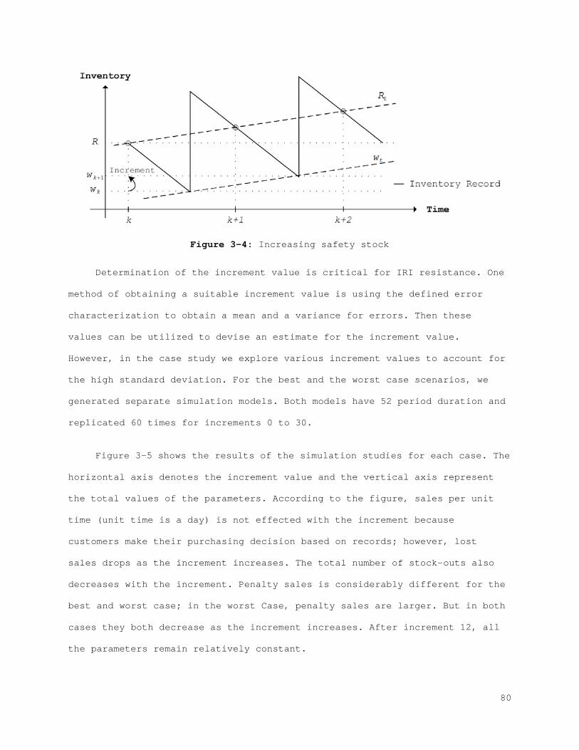
Figure 3-4: Increasing safety stock
Determination of the increment value is critical for IRI resistance. One
method of obtaining a suitable increment value is using the defined error
characterization to obtain a mean and a variance for errors. Then these
values can be utilized to devise an estimate for the increment value.
However, in the case study we explore various increment values to account for
the high standard deviation. For the best and the worst case scenarios, we
generated separate simulation models. Both models have 52 period duration and
replicated 60 times for increments 0 to 30.
Figure 3-5 shows the results of the simulation studies for each case. The
horizontal axis denotes the increment value and the vertical axis represent
the total values of the parameters. According to the figure, sales per unit
time (unit time is a day) is not effected with the increment because
customers make their purchasing decision based on records; however, lost
sales drops as the increment increases. The total number of stock-outs also
decreases with the increment. Penalty sales is considerably different for the
best and worst case; in the worst Case, penalty sales are larger. But in both
cases they both decrease as the increment increases. After increment 12, all
the parameters remain relatively constant.
80
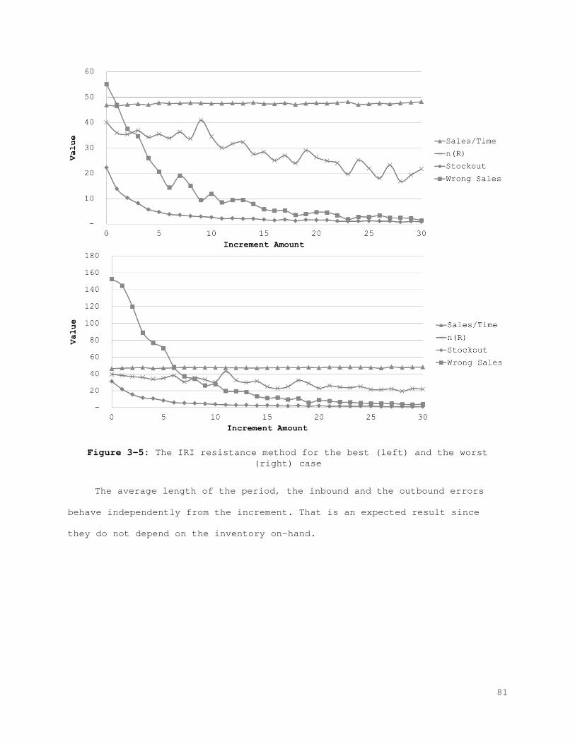
Figure 3-5: The IRI resistance method for the best (left) and the worst (right) case
The average length of the period, the inbound and the outbound errors
behave independently from the increment. That is an expected result since
they do not depend on the inventory on-hand.
81
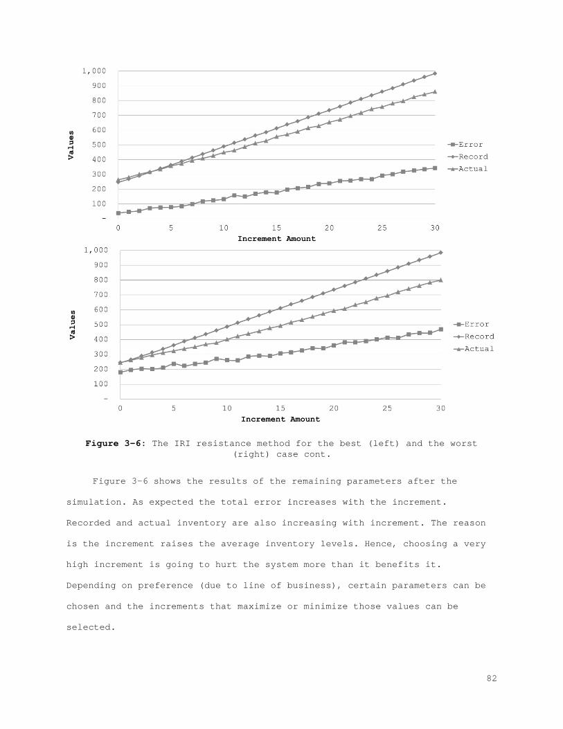
Figure 3-6: The IRI resistance method for the best (left) and the worst (right) case cont.
Figure 3-6 shows the results of the remaining parameters after the
simulation. As expected the total error increases with the increment.
Recorded and actual inventory are also increasing with increment. The reason
is the increment raises the average inventory levels. Hence, choosing a very
high increment is going to hurt the system more than it benefits it.
Depending on preference (due to line of business), certain parameters can be
chosen and the increments that maximize or minimize those values can be
selected.
82
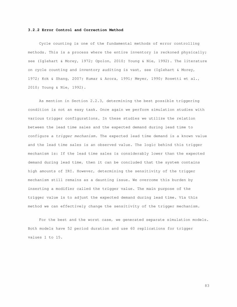
3.2.2 Error Control and Correction Method
Cycle counting is one of the fundamental methods of error controlling
methods. This is a process where the entire inventory is reckoned physically;
see (Iglehart & Morey, 1972; Opolon, 2010; Young & Nie, 1992). The literature
on cycle counting and inventory auditing is vast, see (Iglehart & Morey,
1972; Kok & Shang, 2007; Kumar & Arora, 1991; Meyer, 1990; Rosetti et al.,
2010; Young & Nie, 1992).
As mention in Section 2.2.3, determining the best possible triggering
condition is not an easy task. Once again we perform simulation studies with
various trigger configurations. In these studies we utilize the relation
between the lead time sales and the expected demand during lead time to
configure a trigger mechanism. The expected lead time demand is a known value
and the lead time sales is an observed value. The logic behind this trigger
mechanism is: If the lead time sales is considerably lower than the expected
demand during lead time, then it can be concluded that the system contains
high amounts of IRI. However, determining the sensitivity of the trigger
mechanism still remains as a daunting issue. We overcome this burden by
inserting a modifier called the trigger value. The main purpose of the
trigger value is to adjust the expected demand during lead time. Via this
method we can effectively change the sensitivity of the trigger mechanism.
For the best and the worst case, we generated separate simulation models.
Both models have 52 period duration and use 60 replications for trigger
values 1 to 15.
83
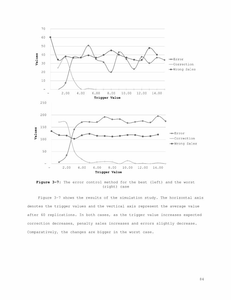
Figure 3-7: The error control method for the best (left) and the worst (right) case
Figure 3-7 shows the results of the simulation study. The horizontal axis
denotes the trigger values and the vertical axis represent the average value
after 60 replications. In both cases, as the trigger value increases expected
correction decreases, penalty sales increases and errors slightly decrease.
Comparatively, the changes are bigger in the worst case.
84
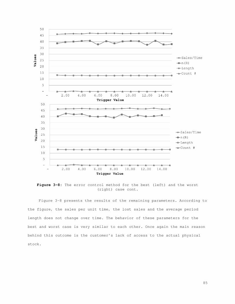
Figure 3-8: The error control method for the best (left) and the worst (right) case cont.
Figure 3-8 presents the results of the remaining parameters. According to
the figure, the sales per unit time, the lost sales and the average period
length does not change over time. The behavior of these parameters for the
best and worst case is very similar to each other. Once again the main reason
behind this outcome is the customer’s lack of access to the actual physical
stock.
85
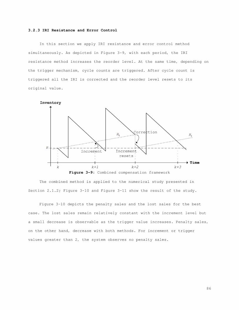
3.2.3 IRI Resistance and Error Control
In this section we apply IRI resistance and error control method
simultaneously. As depicted in Figure 3-9, with each period, the IRI
resistance method increases the reorder level. At the same time, depending on
the trigger mechanism, cycle counts are triggered. After cycle count is
triggered all the IRI is corrected and the reorder level resets to its
original value.
Figure 3-9: Combined compensation framework
The combined method is applied to the numerical study presented in
Section 2.1.2; Figure 3-10 and Figure 3-11 show the result of the study.
Figure 3-10 depicts the penalty sales and the lost sales for the best
case. The lost sales remain relatively constant with the increment level but
a small decrease is observable as the trigger value increases. Penalty sales,
on the other hand, decrease with both methods. For increment or trigger
values greater than 2, the system observes no penalty sales.
86
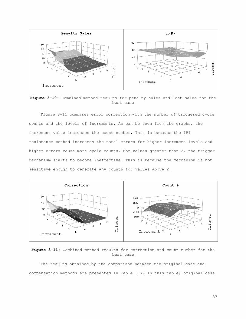
Figure 3-10: Combined method results for penalty sales and lost sales for the best case
Figure 3-11 compares error correction with the number of triggered cycle
counts and the levels of increments. As can be seen from the graphs, the
increment value increases the count number. This is because the IRI
resistance method increases the total errors for higher increment levels and
higher errors cause more cycle counts. For values greater than 2, the trigger
mechanism starts to become ineffective. This is because the mechanism is not
sensitive enough to generate any counts for values above 2.
Figure 3-11: Combined method results for correction and count number for the best case
The results obtained by the comparison between the original case and
compensation methods are presented in Table 3-7. In this table, original case
87
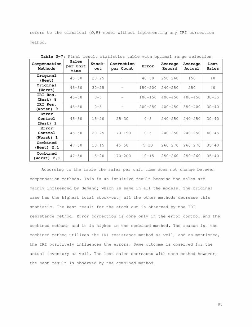
refers to the classical ( ),Q R model without implementing any IRI correction
method.
Table 3-7: Final result statistics table with optimal range selection
Compensation Methods
Sales per unit
time
Stock-out
Correction per Count Error Average
Record Average Actual
Lost Sales
Original (Best) 45-50 20-25 - 40-50 250-260 150 40
Original (Worst) 45-50 30-25 - 150-200 240-250 250 40
IRI Res. (Best) 8 45-50 0-5 - 100-150 400-450 400-450 30-35
IRI Res. (Worst) 9 45-50 0-5 - 200-250 400-450 350-400 30-40
Error Control (Best) 1
45-50 15-20 25-30 0-5 240-250 240-250 30-40
Error Control
(Worst) 1 45-50 20-25 170-190 0-5 240-250 240-250 40-45
Combined (Best) 2,1 47-50 10-15 45-50 5-10 260-270 260-270 35-40
Combined (Worst) 2,1 47-50 15-20 170-200 10-15 250-260 250-260 35-40
According to the table the sales per unit time does not change between
compensation methods. This is an intuitive result because the sales are
mainly influenced by demand; which is same in all the models. The original
case has the highest total stock-out; all the other methods decrease this
statistic. The best result for the stock-out is observed by the IRI
resistance method. Error correction is done only in the error control and the
combined method; and it is higher in the combined method. The reason is, the
combined method utilizes the IRI resistance method as well, and as mentioned,
the IRI positively influences the errors. Same outcome is observed for the
actual inventory as well. The lost sales decreases with each method however,
the best result is observed by the combined method.
88
3.3 Conclusion and Future Work
IRI behavior in the online retail under the influence of demand, supply
and lead time uncertainty is analyzed. Factors contributing to IRI are
defined and formulated. Then, a framework for calculating the errors is
derived in two separate cases: The best and worst case. Then, a numerical
study using simulation is conducted to show the sensitivity of the inventory
replenishment policy to IRI. The highlights can be summarized as;
• In terms of the lead time demand, there is no conclusive result on
the behavior of the error function. Depending on the input
parameters β and δ it can decrease or increase with the lead time
demand.
• In terms of R , w and Y the error function is increasing.
• In both phases the biggest effect is done by the outbound errors.
Hence, the parameter β has the highest impact.
Two alternatives for compensating IRI are presented; the IRI resistance
and the error control method. Then, a numerical analysis is performed to
observe the behavior of IRI and to quantify the effects of the applied
solution alternatives. Based on these studies, the IRI resistance method
positively influences IRI because it increases the average inventory on-hand.
The IRI resistance method performs better on stock-out and lost sales,
whereas the error control method can keep low inventory levels. For the
trigger mechanism high count number means, fewer stock-outs and fewer lost
sales but more frequent counts. Therefore, a range can be chosen and the
values that maximize or minimize desired parameters can be selected.
89
Similar to Chapter 2, the compensation methods described in this chapter
are static. Hence again a good opportunity for future work is utilizing
dynamic correction methods that change for each period.
90
REFERENCES
DeHoratius, N., & Raman, A. (2008). Inventory record inaccuracy: an empirical analysis. Management Science, 54, 627-641.
Erdem, A. S., & Ozekici, S. (2002). Inventory models with random yield in a
random environment. Int. J. Production Economics, 78, 239-253. Grewal, D., Iyer, G. R., & Levy, M. (2004). Internet retailing: enablers,
limiters and market consequences. Journal of Business Research, 57, 703-713.
Henig, M., & Gerchak, Y. (1990). The structure of periodic review in the
presence of random yield. Operations Research, 38, 634-643. Iglehart, D., & Morey, R. C. (1972). Inventory systems with imperfect assest
information. Management Science, 18, 388-394. Kok, A. G., & Shang, K. H. (2007). Inspection and replenishment policies for
systems with inventory record inaccuracy. Manufacturing & Service Operations Management, 9, 185-205.
Kumar, S., & Arora, S. (1991). Development of internal audit and cycle-
counting procedures for reducing inventory miscounts. IIE Transactions, 12, 61-70.
Mangalindan, M. (2005). Online retail sales are expected to rise to $172
billion this year. The Wall Street Journal, 245, D245. Meyer, H. (1990). Inventory accuracy - is it worth it? A case study.
Production and Inventory Management Journal, 31, 15-17. Opolon, D. (2010). Improving product availability in hospitals: the role of
inventory inaccuracies Doctoral dissertation: Massachusetts Institute of Technology.
Rekik, Y., Sahin, E., & Dallery, Y. (2009). Inventory inaccuracy in retail
stores due to theft: An analysis of the benefits of RFID. Int. J. Production Economics, 118, 189-198.
Research, C. f. R. (2005). European Theft Barometer: Monitoring the costs of
Shrinkage and crime for Europe's retailers Centre for Retail Research, Nottingham.
Rosetti, M. D., Buyurgan, N., Bhonsle, A., Gumrukcu, S., & Chittoori., K.
(2010). An analysis of the effect of inventory record inaccuracy in a two-echelon supply chain. Int. J. Inventory Research, 1, 174-208.
Tsay, A. A., & Agrawal, N. (2004). Modeling conflict and coordination in
multi-channel distribution systems: A review. International Series in Operations Research and Management Science, 557-680.
Yan, C., Banerjee, A., & Yang, L. (2011). An integrated production-
distribution model for a deteriorating inventory item. Int. J. Production Economics, 133, 228-232.
91
Young, S. T., & Nie, W. D. (1992). A cycle-count model considering inventory policy and record variance. Production Inventory Management J., 33, 11-16.
92
CHAPTER 4 COMPARATIVE ANALYSIS
In the previous chapters we derived characterizations for error behavior
in online and offline retail environment with random demand, supply and lead
time. Furthermore, we provided compensation methods that limit and control
the impact of IRI and conducted numerical analyses using simulation. In this
chapter we provide a comparative analysis using a cost framework for each
setting. Then, we apply the cost framework to the previously developed
compensation methods. Finally, we demonstrate the results with the same case
study.
We develop a cost model by dividing the general cost structure into three
categories: IRI related costs, penalty costs and operating costs. IRI related
costs are the ones caused by errors. As explained in the previous chapters
they can further be categorized as shelving, inbound and outbound errors. The
inbound and outbound errors are similar in the online and the offline retail
settings. Typically, the inbound errors occur during ordering and receiving
processes whereas the outbound errors occur during check-out processes (e.g.
scanning errors). Shelving errors on the other hand are different for the
online and the offline retail environment. Due to customer interaction in the
offline retail environment, items are subject to theft and spoilage whereas
in the online environment only spoilage occurs.
Penalty costs consist of cycle counting costs and lost sales for the
offline retail setting. In addition to those, the online settings also have
penalty sales. Recall that, penalty sales denote the number of units sold
when the actual inventory is zero but the inventory records are positive (see
Appendix A). Operating costs are typically incurred in routine inventory
management processes: holding, purchasing and selling price (as a negative
93
cost). These are known by the decision maker at all times. Moreover, they are
used as the basis for estimating the remaining cost parameters.
4.1 Model
Let purchasing cost, holding cost for one period, and selling price of
one unit of inventory be c , h, and p , respectively, where 0p c h> > > . The
total cost in the ( ),Q R framework as defined in Zipkin (2000) is,
( ) [ ]( ) [ ] [ ]( )',
2Q E D E D
TC Q R h R E D k n RQ Q
ρ= + − + +
where
( ) { }[ ] ( ) ( )max ,0 DR
n R E D R z R f z dz∞
= − = −∫ .
In the above equations h, k , ρ , 'D and ( )n R are respectively holding,
ordering, shortage cost, lead time, the expected unit time average demand and
the expected lost sales. Additionally, the term [ ]/E D Q denotes the expected
unit time average demand per order (Nahmias, 2008). In our model we modify
this cost function by introducing IRI and penalty cost. The costs are
estimated as follows:
IRI related costs: IRI has two consequences. First of all, the items that
are affected by IRI become unsalable; thus, the opportunity of selling those
items is vanished. The cost of losing the opportunity to sell an item is p .
Secondly, the unsalable items also become unobservable; hence the inventory
replenishment policy receives incorrect information. Finding a cost for
incorrect information is challenging. For practicality, we use λ to represent
the cost of one unit of mismatch between actual inventory and records.
Furthermore, it is possible to experience a positive or negative IRI. In this
context positive IRI corresponds to losing inventory due to shrinkage.
94
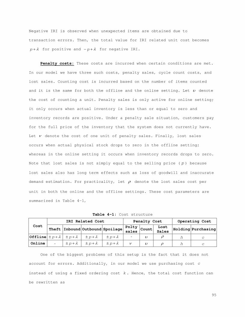
Negative IRI is observed when unexpected items are obtained due to
transaction errors. Then, the total value for IRI related unit cost becomes
p λ+ for positive and p λ− + for negative IRI.
Penalty costs: These costs are incurred when certain conditions are met.
In our model we have three such costs, penalty sales, cycle count costs, and
lost sales. Counting cost is incurred based on the number of items counted
and it is the same for both the offline and the online setting. Let υ denote
the cost of counting a unit. Penalty sales is only active for online setting;
it only occurs when actual inventory is less than or equal to zero and
inventory records are positive. Under a penalty sale situation, customers pay
for the full price of the inventory that the system does not currently have.
Let ν denote the cost of one unit of penalty sales. Finally, lost sales
occurs when actual physical stock drops to zero in the offline setting;
whereas in the online setting it occurs when inventory records drops to zero.
Note that lost sales is not simply equal to the selling price ( p ) because
lost sales also has long term effects such as loss of goodwill and inaccurate
demand estimation. For practicality, let ρ denote the lost sales cost per
unit in both the online and the offline settings. These cost parameters are
summarized in Table 4-1,
Table 4-1: Cost structure
Cost IRI Related Cost Penalty Cost Operating Cost
Theft Inbound Outbound Spoilage Pnlty sales Count Lost Sales Holding Purchasing
Offline p λ± + p λ± + p λ± + p λ± + - υ ρ h c
Online - p λ± + p λ± + p λ± + ν υ ρ h c
One of the biggest problems of this setup is the fact that it does not
account for errors. Additionally, in our model we use purchasing cost c
instead of using a fixed ordering cost k . Hence, the total cost function can
be rewritten as
95
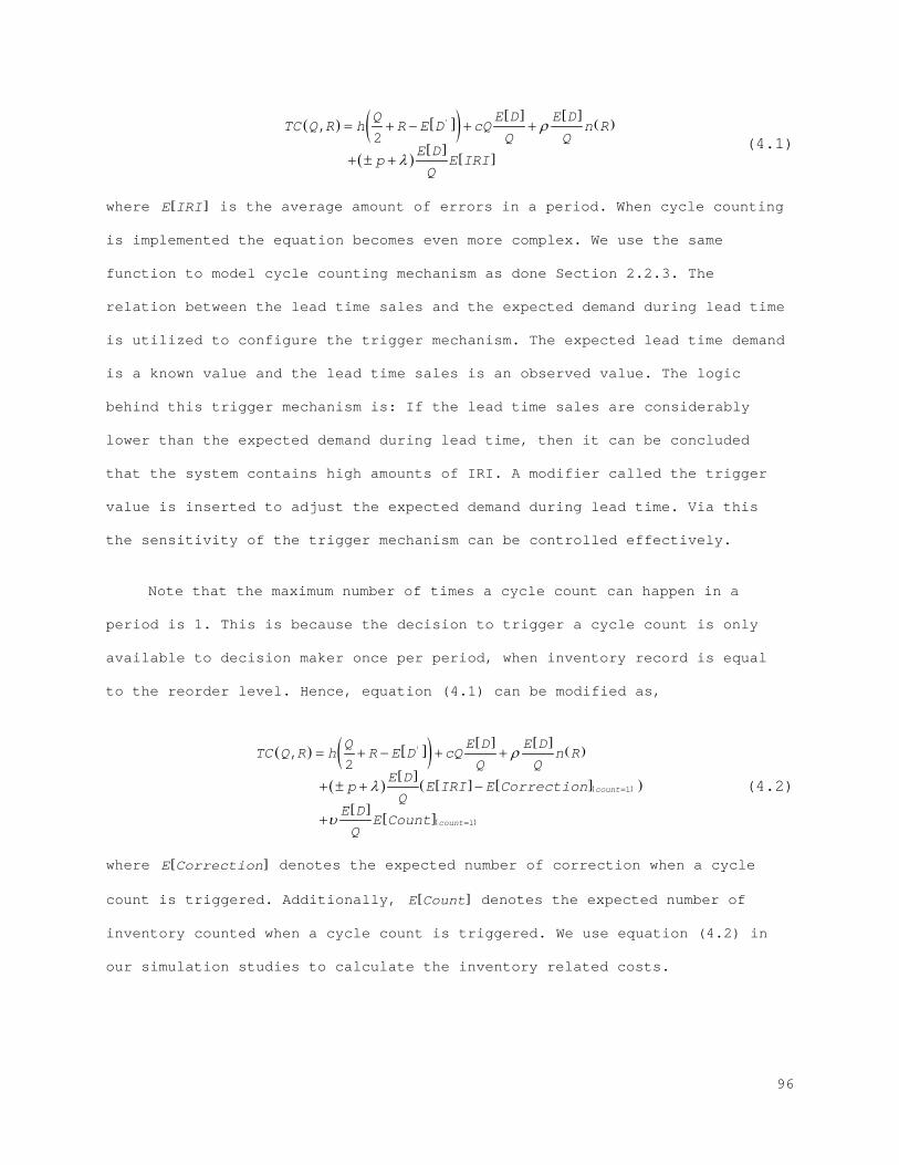
( ) [ ]( ) [ ] [ ]
( )
( )[ ]
[ ]
',2Q E D E D
TC Q R h R E D cQ n RQ Q
E Dp E IRI
Q
ρ
λ
= + − + +
+ ± + (4.1)
where [ ]E IRI is the average amount of errors in a period. When cycle counting
is implemented the equation becomes even more complex. We use the same
function to model cycle counting mechanism as done Section 2.2.3. The
relation between the lead time sales and the expected demand during lead time
is utilized to configure the trigger mechanism. The expected lead time demand
is a known value and the lead time sales is an observed value. The logic
behind this trigger mechanism is: If the lead time sales are considerably
lower than the expected demand during lead time, then it can be concluded
that the system contains high amounts of IRI. A modifier called the trigger
value is inserted to adjust the expected demand during lead time. Via this
the sensitivity of the trigger mechanism can be controlled effectively.
Note that the maximum number of times a cycle count can happen in a
period is 1. This is because the decision to trigger a cycle count is only
available to decision maker once per period, when inventory record is equal
to the reorder level. Hence, equation (4.1) can be modified as,
( ) [ ]( ) [ ] [ ]( )
( )[ ]
[ ] [ ]{ }( )
[ ][ ]{ }
'
1
1
,2
count
count
Q E D E DTC Q R h R E D cQ n R
Q QE D
p E IRI E CorrectionQ
E DE Count
Q
ρ
λ
υ
=
=
= + − + +
+ ± + −
+
(4.2)
where [ ]E Correction denotes the expected number of correction when a cycle
count is triggered. Additionally, [ ]E Count denotes the expected number of
inventory counted when a cycle count is triggered. We use equation (4.2) in
our simulation studies to calculate the inventory related costs.
96
In order to compare similarities and differences of the online and
offline setting we conducted series of simulation studies. We first examine
two groups of studies for the offline setting. The first group is done using
the IRI resistance method (Section 2.2.2); and the second group is done using
the error control method (Section 2.2.3). In both groups several separate
simulation studies are performed to understand the sensitivity of the total
cost with respect to IRI and penalty costs. Furthermore, the best and the
worst case framework are also implemented during these analyses. The same
methodical analyses are then performed for the online setting.
The main goal of these studies is to use the costs as a generic measure
for all the key performance metrics. Then, the total cost function in
equation (4.2) can be used to determine the effectiveness of the compensation
methods described in Chapter 2 and Appendix A.
The simulation study uses the same numerical study in Section 2.1.2. In
the case study, a continuous ( ),Q R policy is utilized with ( )600,80 . Weekly
demand and lead time are normally distributed with ( )250,12 and ( )21.14,0.33
respectively. Parameters for shelving errors are 1%α = and 0.5%β = whereas
parameters for transaction errors are uniformly distributed with [ ]1%,1%δ ∈ −
and [ ]2%,2%γ ∈ − .
4.2 Numerical Study: The Offline Retail Setting
We first discuss the findings for the offline retail environment. Using
the error characterization derived in Chapter 2 and the cost structure
presented equation (4.2) we conducted two groups of simulation studies. The
first group is done to assess the best levels of increment for the IRI
97
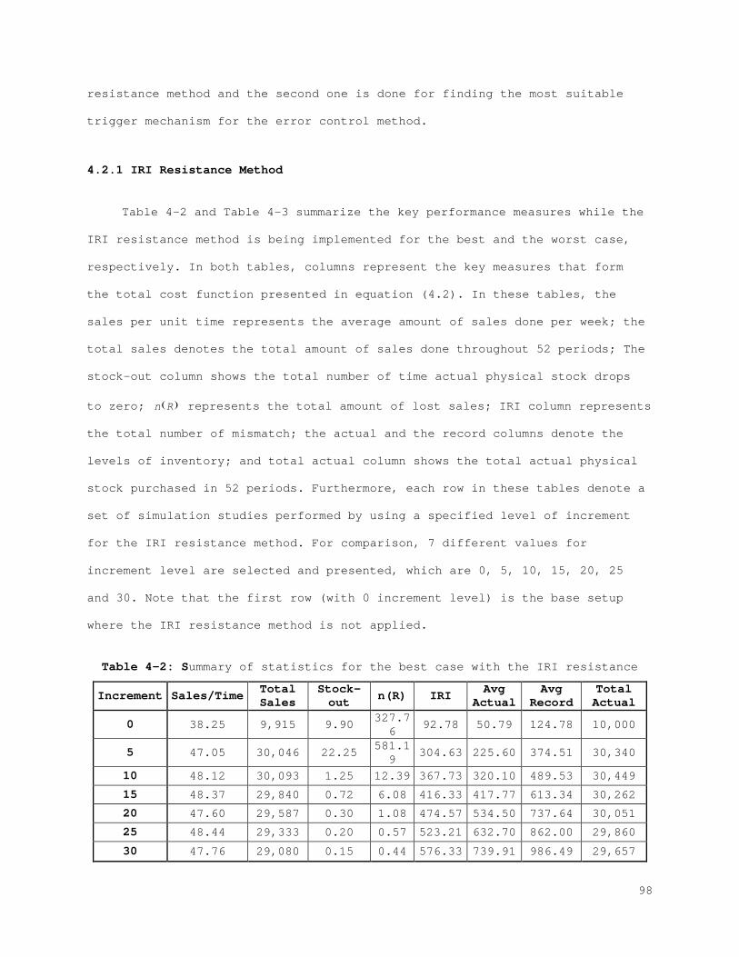
resistance method and the second one is done for finding the most suitable
trigger mechanism for the error control method.
4.2.1 IRI Resistance Method
Table 4-2 and Table 4-3 summarize the key performance measures while the
IRI resistance method is being implemented for the best and the worst case,
respectively. In both tables, columns represent the key measures that form
the total cost function presented in equation (4.2). In these tables, the
sales per unit time represents the average amount of sales done per week; the
total sales denotes the total amount of sales done throughout 52 periods; The
stock-out column shows the total number of time actual physical stock drops
to zero; ( )n R represents the total amount of lost sales; IRI column represents
the total number of mismatch; the actual and the record columns denote the
levels of inventory; and total actual column shows the total actual physical
stock purchased in 52 periods. Furthermore, each row in these tables denote a
set of simulation studies performed by using a specified level of increment
for the IRI resistance method. For comparison, 7 different values for
increment level are selected and presented, which are 0, 5, 10, 15, 20, 25
and 30. Note that the first row (with 0 increment level) is the base setup
where the IRI resistance method is not applied.
Table 4-2: Summary of statistics for the best case with the IRI resistance
Increment Sales/Time Total Sales
Stock-out n(R) IRI Avg
Actual Avg
Record Total Actual
0 38.25 9,915 9.90 327.76
92.78 50.79 124.78 10,000
5 47.05 30,046 22.25 581.19
304.63 225.60 374.51 30,340
10 48.12 30,093 1.25 12.39 367.73 320.10 489.53 30,449
15 48.37 29,840 0.72 6.08 416.33 417.77 613.34 30,262
20 47.60 29,587 0.30 1.08 474.57 534.50 737.64 30,051
25 48.44 29,333 0.20 0.57 523.21 632.70 862.00 29,860
30 47.76 29,080 0.15 0.44 576.33 739.91 986.49 29,657
98
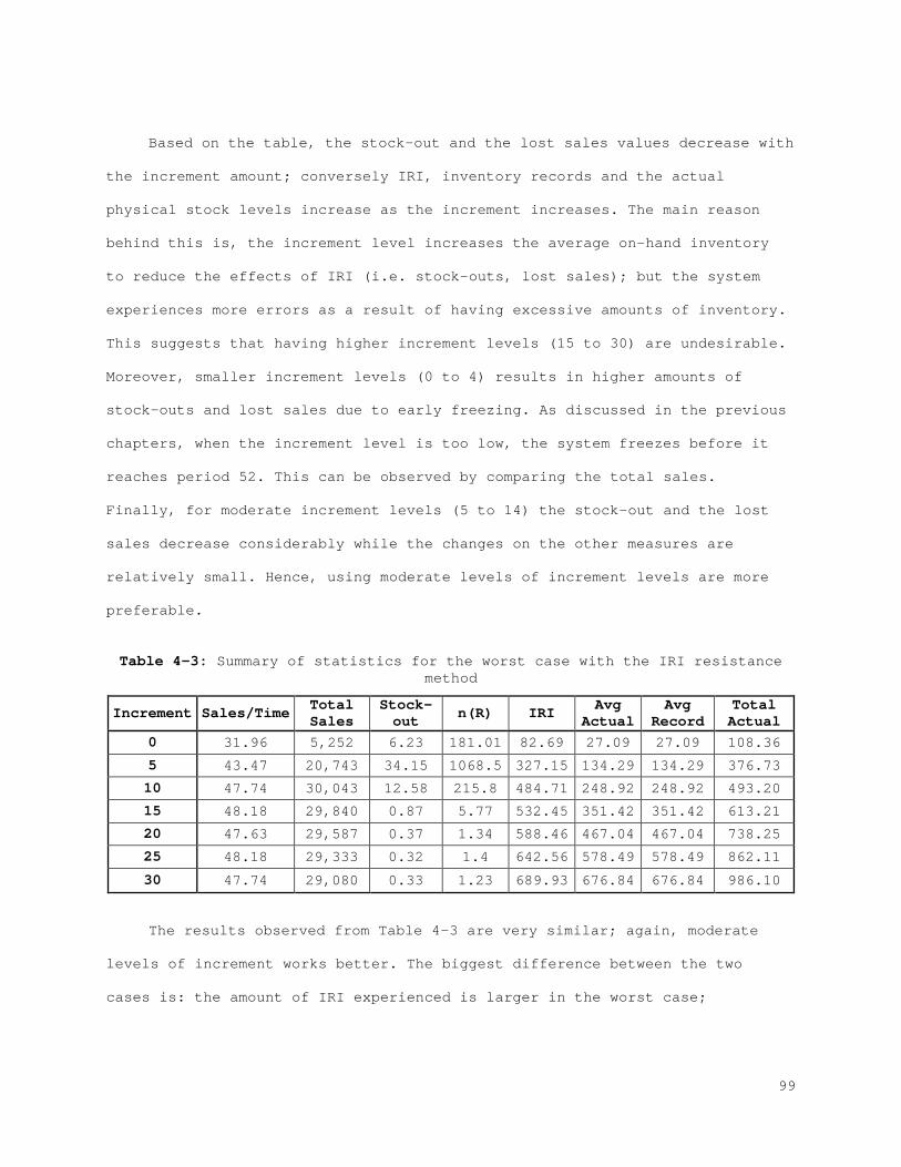
Based on the table, the stock-out and the lost sales values decrease with
the increment amount; conversely IRI, inventory records and the actual
physical stock levels increase as the increment increases. The main reason
behind this is, the increment level increases the average on-hand inventory
to reduce the effects of IRI (i.e. stock-outs, lost sales); but the system
experiences more errors as a result of having excessive amounts of inventory.
This suggests that having higher increment levels (15 to 30) are undesirable.
Moreover, smaller increment levels (0 to 4) results in higher amounts of
stock-outs and lost sales due to early freezing. As discussed in the previous
chapters, when the increment level is too low, the system freezes before it
reaches period 52. This can be observed by comparing the total sales.
Finally, for moderate increment levels (5 to 14) the stock-out and the lost
sales decrease considerably while the changes on the other measures are
relatively small. Hence, using moderate levels of increment levels are more
preferable.
Table 4-3: Summary of statistics for the worst case with the IRI resistance method
Increment Sales/Time Total Sales
Stock-out n(R) IRI Avg
Actual Avg
Record Total Actual
0 31.96 5,252 6.23 181.01 82.69 27.09 27.09 108.36
5 43.47 20,743 34.15 1068.5 327.15 134.29 134.29 376.73
10 47.74 30,043 12.58 215.8 484.71 248.92 248.92 493.20
15 48.18 29,840 0.87 5.77 532.45 351.42 351.42 613.21
20 47.63 29,587 0.37 1.34 588.46 467.04 467.04 738.25
25 48.18 29,333 0.32 1.4 642.56 578.49 578.49 862.11
30 47.74 29,080 0.33 1.23 689.93 676.84 676.84 986.10
The results observed from Table 4-3 are very similar; again, moderate
levels of increment works better. The biggest difference between the two
cases is: the amount of IRI experienced is larger in the worst case;
99
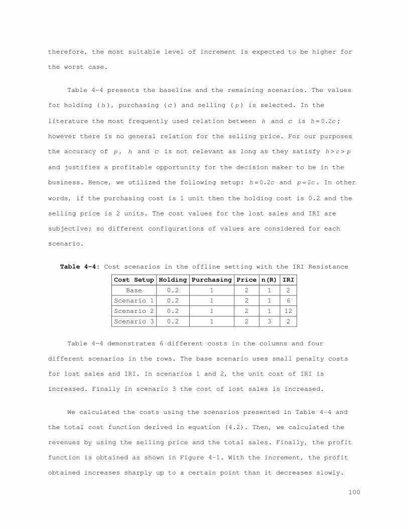
therefore, the most suitable level of increment is expected to be higher for
the worst case.
Table 4-4 presents the baseline and the remaining scenarios. The values
for holding (h ), purchasing (c ) and selling ( p ) is selected. In the
literature the most frequently used relation between h and c is 0.2h c= ;
however there is no general relation for the selling price. For our purposes
the accuracy of p , h and c is not relevant as long as they satisfy h c p> >
and justifies a profitable opportunity for the decision maker to be in the
business. Hence, we utilized the following setup: 0.2h c= and 2p c= . In other
words, if the purchasing cost is 1 unit then the holding cost is 0.2 and the
selling price is 2 units. The cost values for the lost sales and IRI are
subjective; so different configurations of values are considered for each
scenario.
Table 4-4: Cost scenarios in the offline setting with the IRI Resistance
Cost Setup Holding Purchasing Price n(R) IRI
Base 0.2 1 2 1 2
Scenario 1 0.2 1 2 1 6
Scenario 2 0.2 1 2 1 12
Scenario 3 0.2 1 2 3 2
Table 4-4 demonstrates 6 different costs in the columns and four
different scenarios in the rows. The base scenario uses small penalty costs
for lost sales and IRI. In scenarios 1 and 2, the unit cost of IRI is
increased. Finally in scenario 3 the cost of lost sales is increased.
We calculated the costs using the scenarios presented in Table 4-4 and
the total cost function derived in equation (4.2). Then, we calculated the
revenues by using the selling price and the total sales. Finally, the profit
function is obtained as shown in Figure 4-1. With the increment, the profit
obtained increases sharply up to a certain point than it decreases slowly.
100
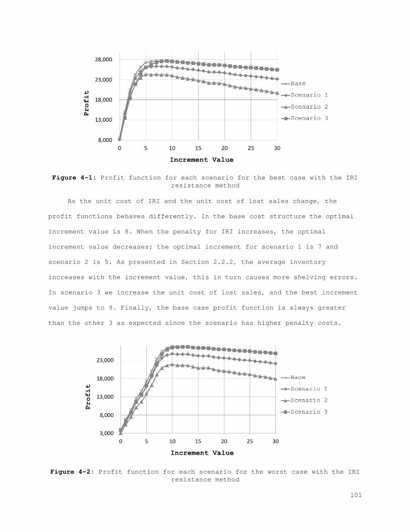
Figure 4-1: Profit function for each scenario for the best case with the IRI resistance method
As the unit cost of IRI and the unit cost of lost sales change, the
profit functions behaves differently. In the base cost structure the optimal
increment value is 8. When the penalty for IRI increases, the optimal
increment value decreases; the optimal increment for scenario 1 is 7 and
scenario 2 is 5. As presented in Section 2.2.2, the average inventory
increases with the increment value, this in turn causes more shelving errors.
In scenario 3 we increase the unit cost of lost sales, and the best increment
value jumps to 9. Finally, the base case profit function is always greater
than the other 3 as expected since the scenario has higher penalty costs.
Figure 4-2: Profit function for each scenario for the worst case with the IRI resistance method
101
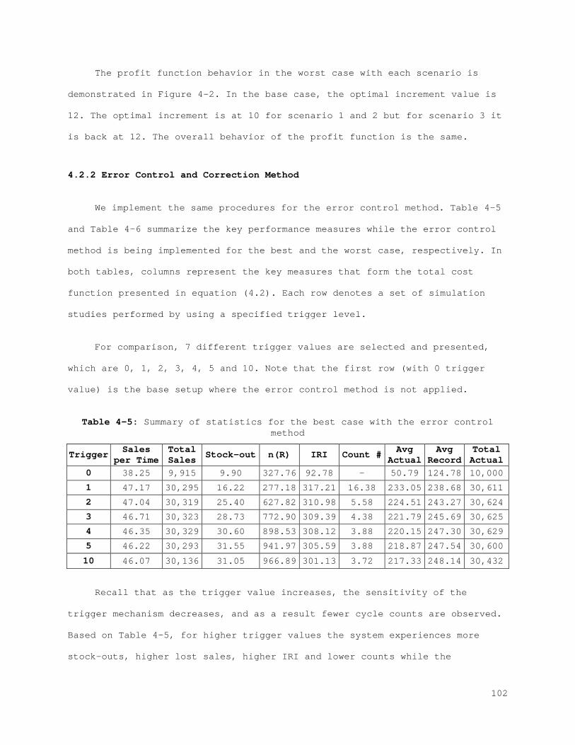
The profit function behavior in the worst case with each scenario is
demonstrated in Figure 4-2. In the base case, the optimal increment value is
12. The optimal increment is at 10 for scenario 1 and 2 but for scenario 3 it
is back at 12. The overall behavior of the profit function is the same.
4.2.2 Error Control and Correction Method
We implement the same procedures for the error control method. Table 4-5
and Table 4-6 summarize the key performance measures while the error control
method is being implemented for the best and the worst case, respectively. In
both tables, columns represent the key measures that form the total cost
function presented in equation (4.2). Each row denotes a set of simulation
studies performed by using a specified trigger level.
For comparison, 7 different trigger values are selected and presented,
which are 0, 1, 2, 3, 4, 5 and 10. Note that the first row (with 0 trigger
value) is the base setup where the error control method is not applied.
Table 4-5: Summary of statistics for the best case with the error control method
Trigger Sales per Time
Total Sales Stock-out n(R) IRI Count # Avg
Actual Avg
Record Total Actual
0 38.25 9,915 9.90 327.76 92.78 - 50.79 124.78 10,000
1 47.17 30,295 16.22 277.18 317.21 16.38 233.05 238.68 30,611
2 47.04 30,319 25.40 627.82 310.98 5.58 224.51 243.27 30,624
3 46.71 30,323 28.73 772.90 309.39 4.38 221.79 245.69 30,625
4 46.35 30,329 30.60 898.53 308.12 3.88 220.15 247.30 30,629
5 46.22 30,293 31.55 941.97 305.59 3.88 218.87 247.54 30,600
10 46.07 30,136 31.05 966.89 301.13 3.72 217.33 248.14 30,432
Recall that as the trigger value increases, the sensitivity of the
trigger mechanism decreases, and as a result fewer cycle counts are observed.
Based on Table 4-5, for higher trigger values the system experiences more
stock-outs, higher lost sales, higher IRI and lower counts while the
102
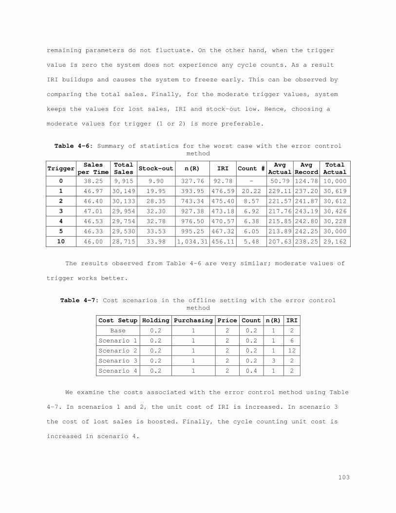
remaining parameters do not fluctuate. On the other hand, when the trigger
value is zero the system does not experience any cycle counts. As a result
IRI buildups and causes the system to freeze early. This can be observed by
comparing the total sales. Finally, for the moderate trigger values, system
keeps the values for lost sales, IRI and stock-out low. Hence, choosing a
moderate values for trigger (1 or 2) is more preferable.
Table 4-6: Summary of statistics for the worst case with the error control method
Trigger Sales per Time
Total Sales Stock-out n(R) IRI Count # Avg
Actual Avg
Record Total Actual
0 38.25 9,915 9.90 327.76 92.78 - 50.79 124.78 10,000
1 46.97 30,149 19.95 393.95 476.59 20.22 229.11 237.20 30,619
2 46.40 30,133 28.35 743.34 475.40 8.57 221.57 241.87 30,612
3 47.01 29,954 32.30 927.38 473.18 6.92 217.76 243.19 30,426
4 46.53 29,754 32.78 976.50 470.57 6.38 215.85 242.80 30,228
5 46.33 29,530 33.53 995.25 467.32 6.05 213.89 242.25 30,000
10 46.00 28,715 33.98 1,034.31 456.11 5.48 207.63 238.25 29,162
The results observed from Table 4-6 are very similar; moderate values of
trigger works better.
Table 4-7: Cost scenarios in the offline setting with the error control method
Cost Setup Holding Purchasing Price Count n(R) IRI
Base 0.2 1 2 0.2 1 2
Scenario 1 0.2 1 2 0.2 1 6
Scenario 2 0.2 1 2 0.2 1 12
Scenario 3 0.2 1 2 0.2 3 2
Scenario 4 0.2 1 2 0.4 1 2
We examine the costs associated with the error control method using Table
4-7. In scenarios 1 and 2, the unit cost of IRI is increased. In scenario 3
the cost of lost sales is boosted. Finally, the cycle counting unit cost is
increased in scenario 4.
103

Figure 4-3 depicts the profit function for each of the cost scenarios for
the best case framework. The behavior of the error control method for
compensating IRI is considerably different from the IRI resistance method. In
the IRI resistance method, with the increment the profit obtained increases
sharply up to a certain point than it decreases slowly. But in this setup,
the change in the profit function is small. But it is still possible to
observe an increasing motion followed by a slow decrease. The recorded
optimal trigger value for both best and worst cost structure is 2. Scenario
1, 2 and 4 does not change the optimal value for both cases but in Scenario 3
the optimal trigger jumps to 3 for both cases.
Figure 4-3: Profit function for each scenario for the best case with the error control method
As demonstrated in previous chapters, when applied, the error control
method brings the best and the worst case setup closer to each other. This
result is clearer in Figure 4-3 and Figure 4-4.
104
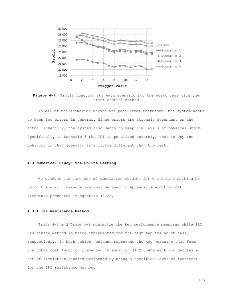
Figure 4-4: Profit function for each scenario for the worst case with the error control method
In all of the scenarios errors are penalized; therefore, the system wants
to keep low errors in general. Since errors are strongly dependent on the
actual inventory, the system also wants to keep low levels of physical stock.
Specifically in Scenario 3 the IRI is penalized severely, that is why the
behavior in that scenario is a little different than the rest.
4.3 Numerical Study: The Online Setting
We conduct the same set of simulation studies for the online setting by
using the error characterizations derived in Appendix A and the cost
structure presented in equation (4.2).
4.3.1 IRI Resistance Method
Table 4-8 and Table 4-9 summarize the key performance measures while IRI
resistance method is being implemented for the best and the worst case,
respectively. In both tables, columns represent the key measures that form
the total cost function presented in equation (4.2). And each row denotes a
set of simulation studies performed by using a specified level of increment
for the IRI resistance method.
105
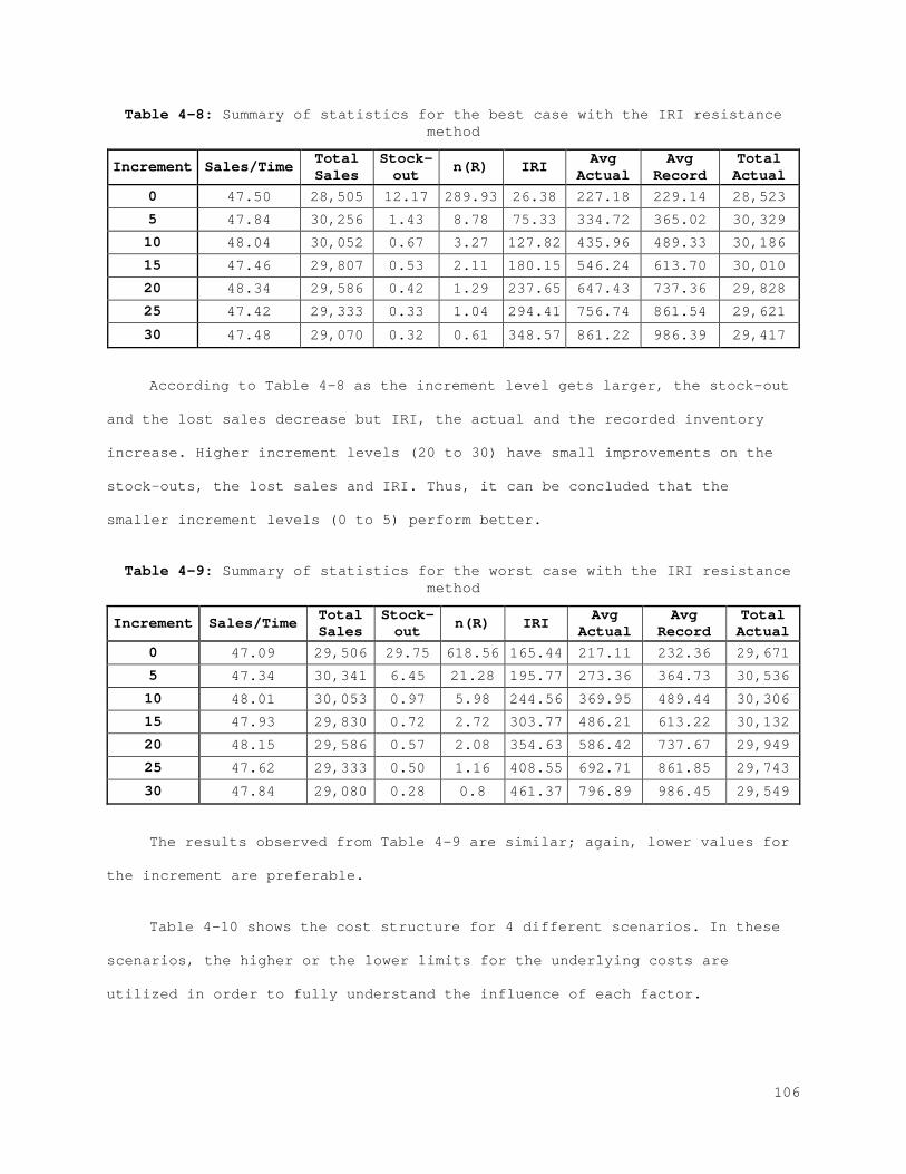
Table 4-8: Summary of statistics for the best case with the IRI resistance method
Increment Sales/Time Total Sales
Stock-out n(R) IRI Avg
Actual Avg
Record Total Actual
0 47.50 28,505 12.17 289.93 26.38 227.18 229.14 28,523
5 47.84 30,256 1.43 8.78 75.33 334.72 365.02 30,329
10 48.04 30,052 0.67 3.27 127.82 435.96 489.33 30,186
15 47.46 29,807 0.53 2.11 180.15 546.24 613.70 30,010
20 48.34 29,586 0.42 1.29 237.65 647.43 737.36 29,828
25 47.42 29,333 0.33 1.04 294.41 756.74 861.54 29,621
30 47.48 29,070 0.32 0.61 348.57 861.22 986.39 29,417
According to Table 4-8 as the increment level gets larger, the stock-out
and the lost sales decrease but IRI, the actual and the recorded inventory
increase. Higher increment levels (20 to 30) have small improvements on the
stock-outs, the lost sales and IRI. Thus, it can be concluded that the
smaller increment levels (0 to 5) perform better.
Table 4-9: Summary of statistics for the worst case with the IRI resistance method
Increment Sales/Time Total Sales
Stock-out n(R) IRI Avg
Actual Avg
Record Total Actual
0 47.09 29,506 29.75 618.56 165.44 217.11 232.36 29,671
5 47.34 30,341 6.45 21.28 195.77 273.36 364.73 30,536
10 48.01 30,053 0.97 5.98 244.56 369.95 489.44 30,306
15 47.93 29,830 0.72 2.72 303.77 486.21 613.22 30,132
20 48.15 29,586 0.57 2.08 354.63 586.42 737.67 29,949
25 47.62 29,333 0.50 1.16 408.55 692.71 861.85 29,743
30 47.84 29,080 0.28 0.8 461.37 796.89 986.45 29,549
The results observed from Table 4-9 are similar; again, lower values for
the increment are preferable.
Table 4-10 shows the cost structure for 4 different scenarios. In these
scenarios, the higher or the lower limits for the underlying costs are
utilized in order to fully understand the influence of each factor.
106
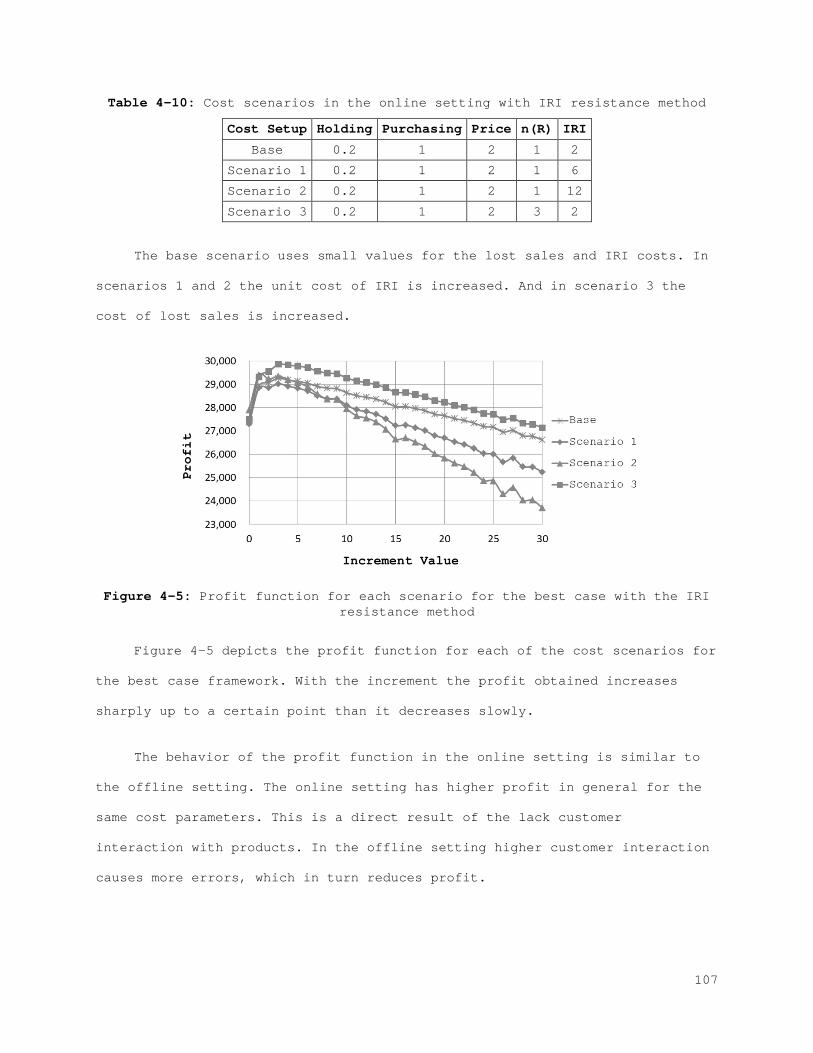
Table 4-10: Cost scenarios in the online setting with IRI resistance method
Cost Setup Holding Purchasing Price n(R) IRI
Base 0.2 1 2 1 2
Scenario 1 0.2 1 2 1 6
Scenario 2 0.2 1 2 1 12
Scenario 3 0.2 1 2 3 2
The base scenario uses small values for the lost sales and IRI costs. In
scenarios 1 and 2 the unit cost of IRI is increased. And in scenario 3 the
cost of lost sales is increased.
Figure 4-5: Profit function for each scenario for the best case with the IRI resistance method
Figure 4-5 depicts the profit function for each of the cost scenarios for
the best case framework. With the increment the profit obtained increases
sharply up to a certain point than it decreases slowly.
The behavior of the profit function in the online setting is similar to
the offline setting. The online setting has higher profit in general for the
same cost parameters. This is a direct result of the lack customer
interaction with products. In the offline setting higher customer interaction
causes more errors, which in turn reduces profit.
107
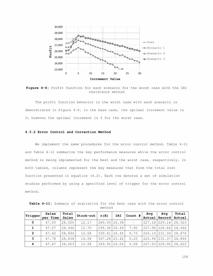
Figure 4-6: Profit function for each scenario for the worst case with the IRI resistance method
The profit function behavior in the worst case with each scenario is
demonstrated in Figure 4-6. In the base case, the optimal increment value is
3; however the optimal increment is 5 for the worst case.
4.3.2 Error Control and Correction Method
We implement the same procedures for the error control method. Table 4-11
and Table 4-12 summarize the key performance measures while the error control
method is being implemented for the best and the worst case, respectively. In
both tables, columns represent the key measures that form the total cost
function presented in equation (4.2). Each row denotes a set of simulation
studies performed by using a specified level of trigger for the error control
method.
Table 4-11: Summary of statistics for the best case with the error control method
Trigger Sales per Time
Total Sales Stock-out n(R) IRI Count # Avg
Actual Avg
Record Total Actual
0 47.50 28,505 12.17 289.93 26.38 - 227.18 229.14 28,523
1 47.57 28,446 12.70 295.38 26.44 7.90 227.96 228.86 28,466
2 47.42 28,844 12.58 330.41 26.45 0.73 226.14 231.34 28,876
3 47.78 28,838 14.58 367.28 25.42 0.25 225.96 231.37 28,866
4 47.47 28,603 12.58 349.92 26.06 0.08 227.53 229.00 28,622
108
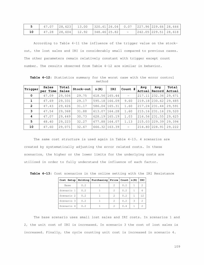
5 47.07 28,623 13.00 320.41 26.04 0.07 227.96 229.66 28,644
10 47.28 28,604 12.92 348.46 25.82 - 242.05 229.51 28,618
According to Table 4-11 the influence of the trigger value on the stock-
out, the lost sales and IRI is considerably small compared to previous cases.
The other parameters remain relatively constant with trigger except count
number. The results observed from Table 4-12 are similar in behavior.
Table 4-12: Statistics summary for the worst case with the error control method
Trigger Sales per Time
Total Sales Stock-out n(R) IRI Count # Avg
Actual Avg
Record Total Actual
0 47.09 29,506 29.75 618.56 165.44 - 217.11 232.36 29,671
1 47.69 29,331 29.17 595.18 166.09 9.60 219.18 230.62 29,485
2 47.43 29,426 31.17 586.04 165.31 1.60 217.24 231.44 29,591
3 47.54 29,368 31.88 613.07 164.28 1.60 215.16 231.16 29,520
4 47.07 29,449 30.73 628.19 165.19 1.03 216.56 231.55 29,625
5 48.40 29,223 32.27 677.88 164.07 1.13 215.03 229.39 29,394
10 47.60 29,071 32.67 666.32 163.39 - 214.80 228.91 29,222
The same cost structure is used again in Table 4-13. 4 scenarios are
created by systematically adjusting the error related costs. In these
scenarios, the higher or the lower limits for the underlying costs are
utilized in order to fully understand the influence of each factor.
Table 4-13: Cost scenarios in the online setting with the IRI Resistance
Cost Setup Holding Purchasing Price Count n(R) IRI
Base 0.2 1 2 0.2 1 2
Scenario 1 0.2 1 2 0.2 1 6
Scenario 2 0.2 1 2 0.2 1 12
Scenario 3 0.2 1 2 0.2 3 2
Scenario 4 0.2 1 2 0.4 1 2
The base scenario uses small lost sales and IRI costs. In scenarios 1 and
2, the unit cost of IRI is increased. In scenario 3 the cost of lost sales is
increased. Finally, the cycle counting unit cost is increased in scenario 4.
109
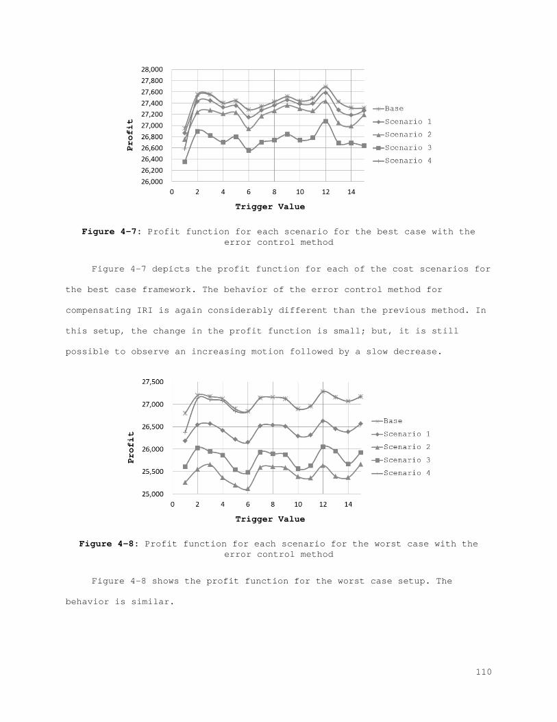
Figure 4-7: Profit function for each scenario for the best case with the error control method
Figure 4-7 depicts the profit function for each of the cost scenarios for
the best case framework. The behavior of the error control method for
compensating IRI is again considerably different than the previous method. In
this setup, the change in the profit function is small; but, it is still
possible to observe an increasing motion followed by a slow decrease.
Figure 4-8: Profit function for each scenario for the worst case with the error control method
Figure 4-8 shows the profit function for the worst case setup. The
behavior is similar.
110
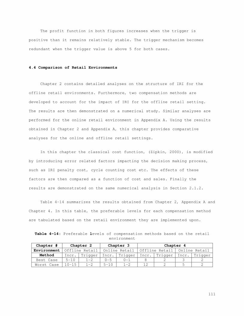
The profit function in both figures increases when the trigger is
positive than it remains relatively stable. The trigger mechanism becomes
redundant when the trigger value is above 5 for both cases.
4.4 Comparison of Retail Environments
Chapter 2 contains detailed analyses on the structure of IRI for the
offline retail environments. Furthermore, two compensation methods are
developed to account for the impact of IRI for the offline retail setting.
The results are then demonstrated on a numerical study. Similar analyses are
performed for the online retail environment in Appendix A. Using the results
obtained in Chapter 2 and Appendix A, this chapter provides comparative
analyses for the online and offline retail settings.
In this chapter the classical cost function, (Zipkin, 2000), is modified
by introducing error related factors impacting the decision making process,
such as IRI penalty cost, cycle counting cost etc. The effects of these
factors are then compared as a function of cost and sales. Finally the
results are demonstrated on the same numerical analysis in Section 2.1.2.
Table 4-14 summarizes the results obtained from Chapter 2, Appendix A and
Chapter 4. In this table, the preferable levels for each compensation method
are tabulated based on the retail environment they are implemented upon.
Table 4-14: Preferable levels of compensation methods based on the retail environment
Chapter # Chapter 2 Chapter 3 Chapter 4 Environment Offline Retail Online Retail Offline Retail Online Retail
Method Incr. Trigger Incr. Trigger Incr. Trigger Incr. Trigger Best Case 5-10 1-2 0-5 0-1 8 2 3 2 Worst Case 10-15 1-2 5-10 1-2 12 2 5 2
111
Remark: The results in Chapter 2 and Appendix A do not utilize the cost
structure introduced in this chapter.
Investigations in Chapter 2 and Appendix A show that the IRI resistance
method performs better on keeping stock-out and lost sales low, whereas the
error control method can operate with lower inventory. However, when the cost
structure is implemented then same behavior cannot be observed. Based on the
results obtained in this chapter, IRI resistance method reaches higher profit
values in all of the cases, especially in the online setting.
The overall results of the analyses done in this chapter are summarized
into three groups: Retail environments, compensation methods, and IRI
sensitivity
4.5 Retail environments
Major difference between the online and the offline retail environments
is the lack of customer access to the goods during purchase. This difference
has three major outcomes that greatly affect the inventory model. First, as a
direct result, customers make their purchasing decisions based on the
recorded inventory. This setup increases the importance of record accuracy
and also creates a new type of IRI measure called the penalty sales. Second,
the lack of customer access results in the absence of certain error factors
that are present in the offline setting, such as theft. Because of this, the
preferable levels for each compensation method is lower in the online setting
as can be seen from Table 4-14. Finally, one of the biggest challenges faced
in the offline setting is freezing as described in Section 2.2.1. The online
setting on the other hand, is completely resistant to freezing. The main
reason is, freezing can only occur during a stock-out and in the online
setting these stock-outs are observable.
112
Compensation methods
The profit obtained with the IRI resistance method, in all situations,
increases with the increment level first and then decreases. This suggests
that there is a range of values preferable for the increment value as shown
in Table 4-14.
Also the error control method becomes ineffective in the online setting.
Intuitively, in the error control method the main goal is managing the
difference between the actual and recorded inventory. But in the online
setting, customers use records instead of actual physical stock. As a result
the error control method loses its effectiveness.
IRI sensitivity
The behavior of the profit function under different scenarios is depicted
in Figure 4-1 to Figure 4-8. According to these graphs, the IRI resistance
method is not sensitive to changes in lost sales and unit IRI costs.
Different cost values just change the magnitude of the profit function not
the behavior. In both settings the influence of IRI is much greater than lost
sales, mainly because the IRI resistance method operates with low lost sales.
The profit function movement when the error control method is implemented
shows greater sensitivity to changes in lost sales and IRI unit costs. The
counting cost has small effect on the magnitude of the profit function.
Whereas, lost sales and IRI costs are considerably influential. Moreover,
slight changes in the behavior of the profit function are observed upon
increasing the lost sales cost. This outcome is intuitively because error
control method operated with high lost sales.
113
REFERENCES
Nahmias, S. n. (2008). Production and Operations Analysis. Boston: Sixth ed McGraw-Hill/Irwin.
Zipkin, P. H. (2000). Foundations of inventory management. New York: McGraw-
Hill.
114
CHAPTER 5 FUZZY MULTI-OBJECTIVE MDP MODEL FOR INVENTORY RECORD INACCURACY
Supply chains suffer greatly from inventory inaccuracy, which is a well-
studied problem in the literature. Due to this inaccuracy, the complete
information about the current state of the inventory does not always exist.
In the literature this issue is often referred as inventory visibility. In
this study we concentrate on investigating the value of visibility through
methodically analyzing the benefits of using a secondary source of
information (i.e., automated data capturing) along with traditional inventory
record keeping methods to control the effects of inventory record inaccuracy
(IRI).
In order to fully understand the value of visibility we define a
secondary source of information which is referred to as visibility
information for the rest of this study. We assume that the visibility
information is obtained through an automated data capturing system which may
or may not work with 100% accuracy. Hence the inventory manager has access to
the conventional records and the new visibility data while making decisions.
The inventory management and supply chain related problems are known to
have a complex structure for optimization purposes. The conventional approach
to solve these problems generally involves a cost estimation to bring the key
metrics such as stock-outs, lost sales, or holding etc. to one generic
platform, dollar value. Then an objective function is defined by assigning
scalar weights to these metrics. In the multi-objective setting, the decision
maker tries to optimize two or more objectives simultaneously under various
restrictions. For a multi-objective optimization problem, a complete optimal
solution seldom exists, and a Pareto-optimal solution is usually used. A
number of methods, such as weighting method, assigning priorities to the
115
objectives and setting aspiration levels for the objectives are used to
derive a compromise solution (Rosenthal, 1985).
In general, inventory models involve uncertainty since certain values
like shortage, or penalty cost are not known exactly. Furthermore, the
decision maker often has vague goals such as keeping the shortage costs to a
minimal, or keeping the customers satisfied. For such cases, fuzzy set theory
and fuzzy mathematical programing methods are suitable (Bellman & Zadeh,
1970; Zimmermann, 1978).
In this study, in order to put more emphasis on the effects of IRI, a new
measure is developed as inventory performance by combining four key
performance metrics: lost sales, amount of correction, fill rate and amount
of inventory counted. These key metrics are combined under a unitless
platform using fuzzy logic and combined through additive methods. In a single
item infinite horizon setting we develop a fuzzy multi-objective inventory
model influenced by IRI with cycle counting under random supply, demand and
lead time with no backordering. The multi-objective setup for fuzzy goals, on
the other hand, is formulated using a fuzzy goal programming (FGP) approach
involving different importance levels. Fuzzified goals are then assigned
weights and combined using an additive model to maximize the sum of all the
fuzzy goals. Extra information on additive methods in inventory problems can
be found in Xu and Liu (2008) and Wee et al. (2009).
Our goals are (1) to define an inventory system to assess the value of
visibility, (2) to apply cycle counting methods to the new inventory system
in order to gauge the IRI susceptibility of the created system, (3) to create
a new performance measure (inventory performance) which combines the key
inventory metrics in a platform where they can be compared, and (4) to find
the optimal policy that maximizes the inventory performance
116
The inventory problem is modeled as an infinite horizon discrete-time
discounted Markov decision process with fuzzified multi-objective subjected
to random demand, supply and lead time. This model is extensively analyzed to
understand the optimal policy structure. Finally, a numerical example is
solved using policy iteration algorithm to provide insights.
5.1 Model
Earlier studies the inventory problem is commonly perceived as a
sequential decision making problem. In such a problem, at a specified time
the decision maker observes the state of a system. Based on this state
decision maker chooses an action and receives an immediate reward. The action
choice produces results and the system evolves to a new state at a different
point in time according to a probability distribution determined by the
action choice. Therefore, the main goal is to find a policy that provides a
prescription for choosing actions in any possible future states. In this
study we focus on a particular sequential decision model referred to as
Markov decision process (MDP). In MPDs the set of available actions, the
rewards and the transition probabilities depend only on the current state and
action. Please refer to Puterman (2009).
In inventory problems various types of uncertainties and imprecisions are
inherent; such as demand, supply and lead time randomness. These are often
modeled using approaches from the probability theory. Yet, it is not always
possible to treat all types of uncertainties by probabilistic models (i.e.
shortage cost, stock-out cost etc.). For such imprecise parameters we use
fuzzy numbers defined on bounded intervals on the axis of real numbers. The
fuzziness in inventory models can be present on multiple levels such as
decision variables (S. P. Chen, 2011), costs (Vujosevic et al., 1996), goals
117
(L. H. Chen & Tsai, 2001), parameters (Ouyang & Chang, 2002) or objectives
Wee et al. (2009).
Fuzzy set theory, introduced by Zadeh (1965), is an extension of
traditional set theory. In fuzzy theory the elements of the set are no longer
required to belong to the set; instead, these elements have a degree of
membership that quantifies how well they belong to the set. Fuzzy sets use a
membership function, Aµ , for a set A , that extends the range of { }: 0,1Af U →
to [ ]: 0,1A Uµ → (Kosko, 1992). Triangular and trapezoidal membership function
are very commonly used because they fit most of the cases and provide fast
computation time (Xexéo). Other curves like Gaussian and sigmoid may provide
smooth results but require higher computation time.
The goal of finding the optimal Q and R values have been studied
extensively and therefore not in our scope. Instead we analyze alternatives
that will maximize the potential of the selected ( ),Q R policy by managing IRI.
We are formulating a single-item multi-objective continuous-time stochastic
inventory problem over an infinite horizon where the decision maker is
following a ( ),Q R policy with random lead time, random supply, lost sales and
unobservable IRI. The inventory problem is modeled as an infinite horizon MDP
with multiple objectives with the components discussed below. The multi-
objective setup is defined as the overall inventory performance which is a
combination of four fuzzy parameters: Lost sales, expected error correction,
service level and expected amount counted. These parameters are represented
with triangular membership functions and combined together using fuzzy
additive goal programming. A similar approach is present in Wee et al.
(2009).
118
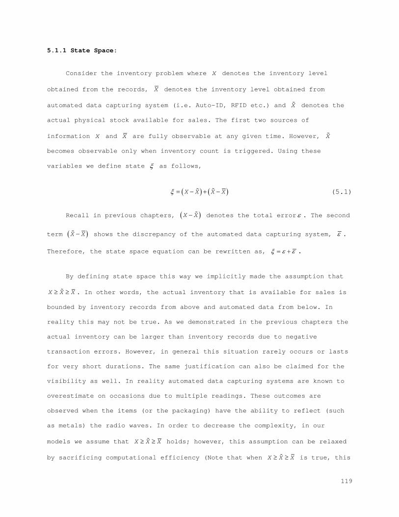
5.1.1 State Space:
Consider the inventory problem where X denotes the inventory level
obtained from the records, X denotes the inventory level obtained from
automated data capturing system (i.e. Auto-ID, RFID etc.) and X denotes the
actual physical stock available for sales. The first two sources of
information X and X are fully observable at any given time. However, X
becomes observable only when inventory count is triggered. Using these
variables we define state ξ as follows,
( ) ( )X X X Xξ = − + − (5.1)
Recall in previous chapters, ( )X X− denotes the total error ε . The second
term ( )X X− shows the discrepancy of the automated data capturing system, ε .
Therefore, the state space equation can be rewritten as, ξ ε ε= + .
By defining state space this way we implicitly made the assumption that
X X X≥ ≥ . In other words, the actual inventory that is available for sales is
bounded by inventory records from above and automated data from below. In
reality this may not be true. As we demonstrated in the previous chapters the
actual inventory can be larger than inventory records due to negative
transaction errors. However, in general this situation rarely occurs or lasts
for very short durations. The same justification can also be claimed for the
visibility as well. In reality automated data capturing systems are known to
overestimate on occasions due to multiple readings. These outcomes are
observed when the items (or the packaging) have the ability to reflect (such
as metals) the radio waves. In order to decrease the complexity, in our
models we assume that X X X≥ ≥ holds; however, this assumption can be relaxed
by sacrificing computational efficiency (Note that when X X X≥ ≥ is true, this
119
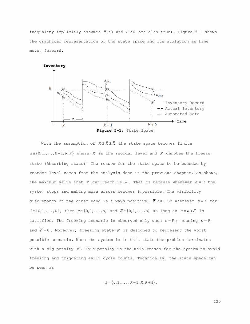
inequality implicitly assumes 0ε ≥ and 0ε ≥ are also true). Figure 5-1 shows
the graphical representation of the state space and its evolution as time
moves forward.
Figure 5-1: State Space
With the assumption of X X X≥ ≥ the state space becomes finite,
{ }0,1,..., 1, ,s R R F∈ − where R is the reorder level and F denotes the freeze
state (Absorbing state). The reason for the state space to be bounded by
reorder level comes from the analysis done in the previous chapter. As shown,
the maximum value that ε can reach is R . That is because whenever Rε = the
system stops and making more errors becomes impossible. The visibility
discrepancy on the other hand is always positive, 0ε ≥ . So whenever s i= for
{ }0,1,...,i R∈ , then { }0,1,...,Rε ∈ and { }0,1,...,Rε ∈ as long as s ε ε= + is
satisfied. The freezing scenario is observed only when s F= ; meaning Rε =
and 0ε = . Moreover, freezing state F is designed to represent the worst
possible scenario. When the system is in this state the problem terminates
with a big penalty m . This penalty is the main reason for the system to avoid
freezing and triggering early cycle counts. Technically, the state space can
be seen as
{ }0,1,..., 1, , 1S R R R= − + .
120
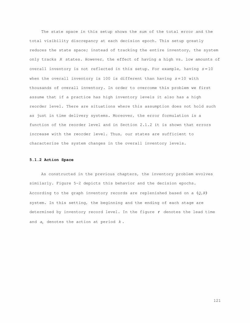
The state space in this setup shows the sum of the total error and the
total visibility discrepancy at each decision epoch. This setup greatly
reduces the state space; instead of tracking the entire inventory, the system
only tracks R states. However, the effect of having a high vs. low amounts of
overall inventory is not reflected in this setup. For example, having 10s =
when the overall inventory is 100 is different than having 10s = with
thousands of overall inventory. In order to overcome this problem we first
assume that if a practice has high inventory levels it also has a high
reorder level. There are situations where this assumption does not hold such
as just in time delivery systems. Moreover, the error formulation is a
function of the reorder level and in Section 2.1.2 it is shown that errors
increase with the reorder level. Thus, our states are sufficient to
characterize the system changes in the overall inventory levels.
5.1.2 Action Space
As constructed in the previous chapters, the inventory problem evolves
similarly. Figure 5-2 depicts this behavior and the decision epochs.
According to the graph inventory records are replenished based on a ( ),Q R
system. In this setting, the beginning and the ending of each stage are
determined by inventory record level. In the figure τ denotes the lead time
and ka denotes the action at period k .
121
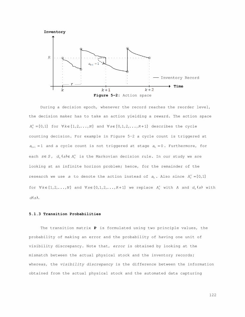
Figure 5-2: Action space
During a decision epoch, whenever the record reaches the reorder level,
the decision maker has to take an action yielding a reward. The action space
{ }0,1ksA = for { }1,2,...,k N∀ ∈ and { }0,1,2,..., 1s R∀ ∈ + describes the cycle
counting decision. For example in Figure 5-2 a cycle count is triggered at
1 1ka + = and a cycle count is not triggered at stage 0ka = . Furthermore, for
each s S∈ , ( ) kk sd s A∈ is the Markovian decision rule. In our study we are
looking at an infinite horizon problem; hence, for the remainder of the
research we use a to denote the action instead of ka . Also since { }0,1ksA =
for { }1,2,...,k N∀ ∈ and { }0,1,2,..., 1s R∀ ∈ + we replace ksA with A and ( )
kd s with
( ).d s
5.1.3 Transition Probabilities
The transition matrix P is formulated using two principle values, the
probability of making an error and the probability of having one unit of
visibility discrepancy. Note that, error is obtained by looking at the
mismatch between the actual physical stock and the inventory records;
whereas, the visibility discrepancy is the difference between the information
obtained from the actual physical stock and the automated data capturing
122
systems. In this study we are interested in maximizing the inventory
performance policy when the system is subjected to IRI.
The error from automated identification systems (i.e. visibility
discrepancy), on the other hand, is dependent on many factors such as item
types, warehouse shape, location, reader distance, packaging and many more.
But we are interested only in the dependency to actual physical stock
available. Although the remaining factors can be important contributions in a
future study, they fall out of this study’s scope. In literature there are
various papers dealing with the capabilities of automated data capturing
systems (Agrawal, 2001; Raman et al., 2001; Ton & Raman, 2004). In our study
we use visibility accuracy as an input parameter that shows the accuracy of
the automated data capturing systems and investigate the various scenarios
involving different levels of visibility accuracy. These levels can be high,
medium and low.
Let ε ′ , ε ′ and s ′ denote the error, visibility discrepancy and the state
space for the next period. Then, ( )0 iP i a gε ε′ − = = ≡ for 0,...,i R= denotes the
probability of having i errors at the current period. In this study we assume
that errors are not corrected unless a cycle count is triggered, which means
0ε ε′ − ≥ is always true. Let ( ), tsP t s a rε = ≡ be the probability of having t
units of visibility discrepancy when the system is in state s where
{ }0,1,...,t R∈ and the action a is taken. Unlike errors, visibility discrepancy
can be automatically corrected. The following condition holds for every s and
t,
( )0
, ts
t sP t s a
r t sε
>= = ≤. (5.2)
To calculate ( ),P s s a′ , we condition on visibility discrepancy
123
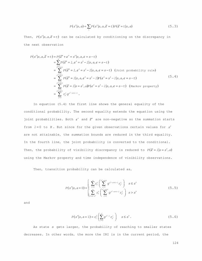
( ) ( ) ( ), , , ,t
P s s a P s s a t P t s aε ε′ ′= = =∑ (5.3)
Then, ( ), ,P s s a tε′ = can be calculated by conditioning on the discrepancy in
the next observation
( ) ( )
( )
( ) ( )
( ) ( )
( ) ( )
0
0
0
0
Joint probability rule
Markov
, , , ,
, , ,
, , ,
, , , ,
, , ,
R
ls s t
ls s t
ls s t
l
P s s a t P s s a s t
P l s l s a s t
P l s l s a s t
P l s a s l P s l s a s t
P l s s a P s l s a s t
ε ε ε ε
ε ε ε
ε ε ε
ε ε ε ε
ε ε ε
=′− +
=′− +
=′− +
=
′ ′ ′ ′= = + = = −
′ ′ ′= = = − = −
′ ′ ′= = = − = −
′ ′ ′ ′ ′= = = − = − = −
′ ′ ′= = = = − = −
∑
∑
∑
∑ ( )
0
property
.s s t
l s s t ls
l
r g′− +
′− + −′
=
= ∑
(5.4)
In equation (5.4) the first line shows the general equality of the
conditional probability. The second equality extends the equation using the
joint probabilities. Both ε ′ and ε ′ are non-negative so the summation starts
from 0l = to R . But since for the given observations certain values for s ′
are not attainable, the summation bounds are reduced in the third equality.
In the fourth line, the joint probability is converted to the conditional.
Then, the probability of visibility discrepancy is reduced to ( ),P l s s aε ′= =
using the Markov property and time independence of visibility observations.
Then, transition probability can be calculated as,
( ) 0 0
0
, 0
s s s tt s s t l ls s
t ls s s t
t s s t l ls s
lt s s
r g r s sP s s a
r g r s s
′− +′− + −
′= =
′− +′− + −
′′ == −
′≤ ′ = = ′>
∑ ∑
∑ ∑ (5.5)
and
( ) 00
0
, 1 s
s l ls
l
P s s a r g r s s′
′−′
=
′ ′= = ≤ ∑ . (5.6)
As state s gets larger, the probability of reaching to smaller states
decreases. In other words, the more the IRI is in the current period, the
124
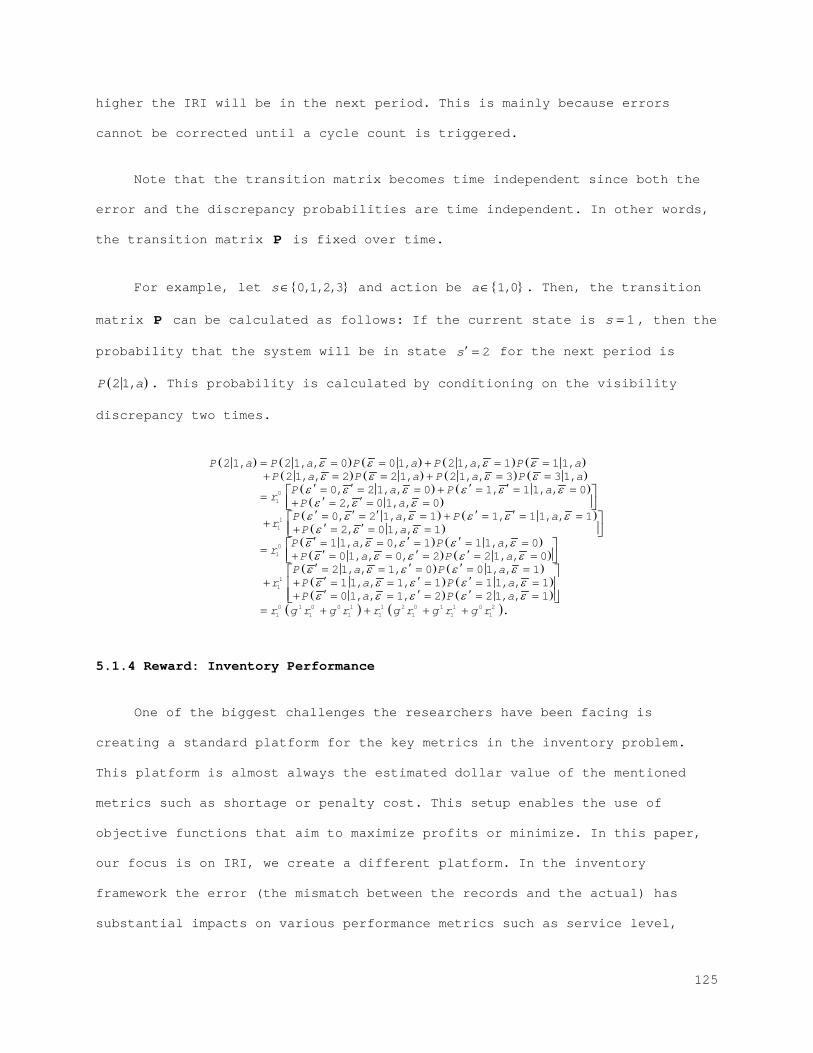
higher the IRI will be in the next period. This is mainly because errors
cannot be corrected until a cycle count is triggered.
Note that the transition matrix becomes time independent since both the
error and the discrepancy probabilities are time independent. In other words,
the transition matrix P is fixed over time.
For example, let { }0,1,2,3s∈ and action be { }1,0a∈ . Then, the transition
matrix P can be calculated as follows: If the current state is 1s = , then the
probability that the system will be in state 2s ′ = for the next period is
( )21,P a . This probability is calculated by conditioning on the visibility
discrepancy two times.
( ) ( ) ( ) ( ) ( )( ) ( ) ( ) ( )
( ) ( )( )
( ) ( )( )
01
11
2 1, 21, , 0 01, 21, , 1 1 1,21, , 2 21, 21, , 3 31,
0, 21, , 0 1, 1 1, , 02, 01, , 0
0, 2 1, , 1 1, 1 1, , 12, 01, , 1
P a P a P a P a P aP a P a P a P a
P a P ar P a
P a P ar P a
ε ε ε εε ε ε ε
ε ε ε ε ε εε ε ε
ε ε ε ε ε εε ε ε
= = = + = =+ = = + = =
′ ′ ′ ′= = = + = = == ′ ′+ = = =′ ′ ′ ′ ′= = = + = = =+ ′ ′+ = = =
( ) ( )( ) ( )
( ) ( )( ) ( )( ) ( )
( )
01
11
0 1 0 0 1 1 2 0 1 11 1 1 1 1 1
1 1, , 0, 1 1 1, , 001, , 0, 2 21, , 021, , 1, 0 01, , 11 1, , 1, 1 1 1, , 101, , 1, 2 21, , 1
P a P ar P a P a
P a P ar P a P a
P a P ar g r g r r g r g r
ε ε ε ε εε ε ε ε ε
ε ε ε ε εε ε ε ε εε ε ε ε ε
′ ′ ′= = = = == ′ ′ ′+ = = = = =′ ′ ′= = = = =′ ′ ′+ + = = = = =′ ′ ′+ = = = = =
= + + +
( )0 21 .g r+
5.1.4 Reward: Inventory Performance
One of the biggest challenges the researchers have been facing is
creating a standard platform for the key metrics in the inventory problem.
This platform is almost always the estimated dollar value of the mentioned
metrics such as shortage or penalty cost. This setup enables the use of
objective functions that aim to maximize profits or minimize. In this paper,
our focus is on IRI, we create a different platform. In the inventory
framework the error (the mismatch between the records and the actual) has
substantial impacts on various performance metrics such as service level,
125
probability of stock-out, average inventory, lost sales, sales, inventory
freezing, cycle counting, error correction, etc. Unfortunately the
traditional models fail to address the importance of all of these metrics at
the same time. Because of this, some of the metrics are constantly
overlooked. By limiting our focus on IRI we limit our research to four key
elements that are directly influenced by errors.
In order to understand the value of errors we develop a new measure
called “inventory performance”. This measure is a combination of the
following metrics, (1) expected lost sales, (2) expected amount of
correction, (3) service level and (4) expected amount of inventory to be
counted. Unfortunately, as mentioned these metrics do not share a uniform
unit. To overcome this challenge we fuzzify each of these metrics into a
unitless platform, combine them into one measure and maximize it.
The correlation between the chosen four performance metrics is
complicated. Based on the simulation analysis presented in the previous
chapters, the following results are concluded: as the frequency of cycle
counting increases (1) the number of correction per count decreases, (2) the
number of stock-outs decreases, (3) lost sales decreases and (4) the total
number of errors made decreases. Additionally, the graphs presented in
pervious chapters show the dependency between these parameters
Theoretically, lost sales is a function of the reorder level, which is a
function of safety stock. And safety stock is a function of service level;
therefore, there is a direct dependency between lost sales and service level.
However, the general characterization for lost sales and service level
assumes that there are no errors. This poses a major problem since the
effects of error on lost sales and service level are very different. Hence,
the correlations between the discussed performance metrics are dependent on
126
the level of errors present in the inventory system. The relation between
correction and the count amount is also similar. That is essentially the
reason why these four metrics are chosen: lost sales, service level, error
correction and count amount.
i. Reward 1: Lost Sales
The first part of the system performance is the lost sales. In the
earlier studies, many inventory models have considered the uncertainty of
shortage costs. However, papers dealing with the fuzzification of shortage
costs are few (Chang et al., 2006; Lin, 2008). In this section, we aim to
fuzzify the value of lost sales. Applications of fuzzy set concepts on EOQ
inventory models have been proposed earlier (Dutta et al., 2007; Vujosevic et
al., 1996; Yao & Chiang, 2003). However, these studies almost always
concentrate on the simple EOQ models, in which restrictive assumptions are
implied.
In a general ( ),Q R setting the expected lost sales is formulated as the
expected number of difference between demand and available inventory for a
specified interval. In other words,
( ) { }[ ] ( ) ( )max ,0 DR
n R E D R z R f z dzτ
∞= − = −∫
where Df is the demand distribution. Note that the term { }max ,0D Rτ − uses
reorder level instead of inventory level. This characterization is possible
due to the decision structure. Recall that decision epochs are identified as
the points at which inventory records reaches reorder level. Since the
decision maker is only allowed to make decisions at decision epochs, the
inventory level can be substituted with reorder level.
127
Lost sales value is generally inserted in the objective function with a
scalar weight p denoting the shortage cost per unit. We utilize a similar
setup for lost sales, where the expected lost sales is calculated with
( ) { }[ ], max ,0 ,n R s a E D R s aτ= − . (5.7)
Equation (5.7) can be rewritten as,
( ){ }[ ]
[ ]{ }[ ]max ,0 1
,max , 1 ,0 0
E D R an R s a
E D R E s a aτ
τ ε− =
= − + = =. (5.8)
Note that in equation (5.8) the second line uses [ ]1E aε = although the
realization is only possible when 0a = . This would seem unintuitive at a quick
glance; however, at any decision epoch for a given s when a cycle count is
not triggered than the actual inventory on-hand is less than or equal to R
(due to IRI). The difference between R and the errors can be estimated by
[ ], 1E s aε = , since it gives the expected amount of error correction if a cycle
count is triggered. Equation (5.10) provides more details on this
calculation.
Then, to describe the fuzzy objective we define an acceptable interval
( ) ( )[ ],l un R n R .
This interval is subjective and it represents the tolerable range for the
lost sales values. The boundary limits ( )ln R and ( )un R , as shown in the Figure
5-3 part A, the optimistic and pessimistic situations respectively.
Naturally, the lower the expected lost sales value is the better. The
membership function ( )( ),n R s aµ , which may be linear or non-linear, is then
used to describe the tolerance rating of the lost sales; the lower the
expected lost sales is, the higher the membership value will be.
128
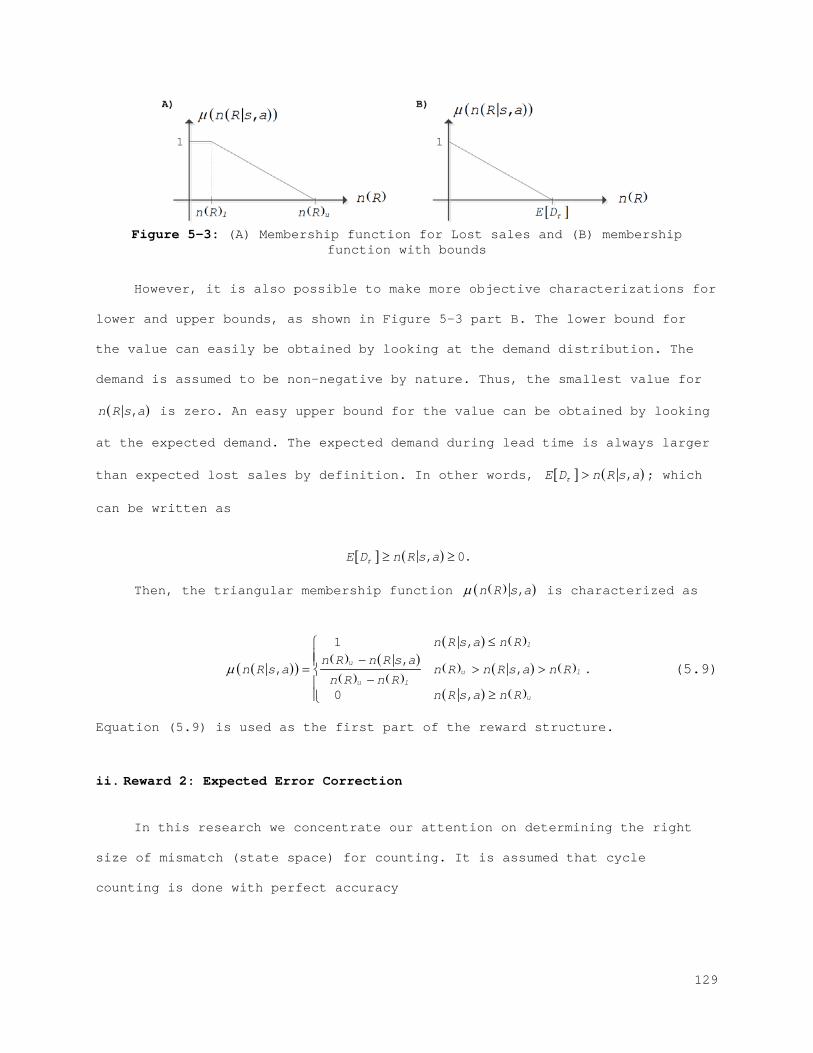
Figure 5-3: (A) Membership function for Lost sales and (B) membership
function with bounds
However, it is also possible to make more objective characterizations for
lower and upper bounds, as shown in Figure 5-3 part B. The lower bound for
the value can easily be obtained by looking at the demand distribution. The
demand is assumed to be non-negative by nature. Thus, the smallest value for
( ),n R s a is zero. An easy upper bound for the value can be obtained by looking
at the expected demand. The expected demand during lead time is always larger
than expected lost sales by definition. In other words, [ ] ( ),E D n R s aτ > ; which
can be written as
[ ] ( ), 0E D n R s aτ ≥ ≥ .
Then, the triangular membership function ( )( ),n R s aµ is characterized as
( )( )
( ) ( )
( ) ( )( ) ( )
( ) ( ) ( )
( ) ( )
1 , ,
, ,
0 ,
l
uu l
u l
u
n R s a n Rn R n R s a
n R s a n R n R s a n Rn R n R
n R s a n R
µ
≤ −
= > >−
≥
. (5.9)
Equation (5.9) is used as the first part of the reward structure.
ii. Reward 2: Expected Error Correction
In this research we concentrate our attention on determining the right
size of mismatch (state space) for counting. It is assumed that cycle
counting is done with perfect accuracy
129
From this perspective, the expected amount of correction can easily be
characterized as
[ ] [ ] 1, 0,1,...,,
0 0 E s a s R
E s aa
εε
= ∀ == = (5.10)
where [ ]E sε is the expected error when the system is in state s upon
triggering the cycle count. Since for a given s and a , [ ] [ ], ,s E s a E s aε ε= + .
Then expected error can be found by conditioning on probability of visibility
discrepancy, or
[ ] ( )
( )
( )
0
0
0
.
s
is
is
i
E s iP i s
iP s i s
iP s i s
ε ε
ε
ε
=
=
=
= =
= − =
= = −
∑
∑
∑
(5.11)
Let ( ) isP i s rε = = , then the above equation can rewritten as,
[ ]0
ss is
i
E s irε −
=
= ∑ . (5.12)
Hence, to describe the fuzzy objective, as shown in Figure 5-4 part A, we
define an acceptable interval [ ] [ ][ ],l uE Eε ε . Naturally, it is better to have
higher values for expected correction. Hence, the triangular membership
function is greater for higher correction values.
The lower bound for the value is zero since the smallest number
correction can get is zero. The upper bound for the value is one since the
maximum correction equals to the reorder level. In other words, as shown in
Figure 5-4 part B the bounds can written as [ ]0 ,E s a Rε≤ ≤ . Figure 5-4 shows
the membership function of fuzzified error correction parameter. For
simplicity we use a triangular membership set as depicted in figure.
130
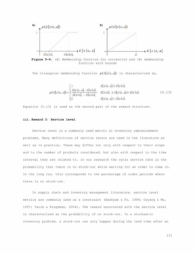
Figure 5-4: (A) Membership function for correction and (B) membership
function with bounds
The triangular membership function [ ]( ),E s aµ ε is characterized as,
[ ]( )
[ ] [ ][ ] [ ]
[ ] [ ][ ] [ ] [ ]
[ ] [ ]
1 ,,
, ,
0 ,
u
ll u
u l
l
E s a E sE s a E s
E s a E s E s a E sE s E s
E s a E s
ε εε ε
µ ε ε ε εε ε
ε ε
≥ −
= ≤ ≤−
<
(5.13)
Equation (5.13) is used as the second part of the reward structure.
iii. Reward 3: Service level
Service level is a commonly used metric in inventory replenishment
problems. Many definitions of service levels are used in the literature as
well as in practice. These may differ not only with respect to their scope
and to the number of products considered, but also with respect to the time
interval they are related to. In our research the cycle service rate is the
probability that there is no stock-out while waiting for an order to come in.
In the long run, this corresponds to the percentage of order periods where
there is no stock-out.
In supply chain and inventory management literature, service level
metrics are commonly used as a constraint (Bashyam & Fu, 1998; Ouyang & Wu,
1997; Tarim & Kingsman, 2004). The reward associated with the service level
is characterized as the probability of no stock-out. In a stochastic
inventory problem, a stock-out can only happen during the lead time after an
131
order is given, assuming that the inventory is not frozen due to errors
(Thiel et al., 2010). Hence, the probability of having no stock-out can be
calculated as,
{ } { } P No Stockout P D Rτ= < .
In this formulation, Dτ denotes the lead time demand. There is a very
definite relationship between service level and the amount of inventory being
stocked. Generally, the more the inventory level is the higher the service
level will be but at a decreasing rate. The traditional setup of safety stock
( )w in ( ),Q R is obtained as follows. Let R w τµ= + be the reorder level where w
is the safety stock and τµ is the lead time demand. Then, w can be formulated
as
* 2 2 2w z µ ττσ µ σ= +.
where τ is the mean lead time, 2µσ is demand variance and 2
τσ is the lead
time variance (Zipkin, 2000). In this formulation *z is the value obtained
from the z -table for the desired service level (complementary type 1 error:
all customer orders arriving within a given time interval will be completely
delivered from stock on-hand). When the lead time is deterministic 2 2τµ σ
becomes zero making * 2w z µτσ= and when there is no lead time w and R becomes
zero. These results are very intuitive because if there is no lead time than
there is no reason to have extra inventory. Obviously, such generalizations
have limited viability in practice. Due to the difficulty in characterization
of safety stock, in general the service level commonly becomes an input
parameter inserted as a constraint.
132
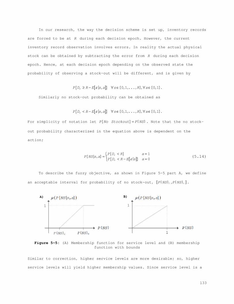
In our research, the way the decision scheme is set up, inventory records
are forced to be at R during each decision epoch. However, the current
inventory record observation involves errors. In reality the actual physical
stock can be obtained by subtracting the error from R during each decision
epoch. Hence, at each decision epoch depending on the observed state the
probability of observing a stock-out will be different, and is given by
[ ]{ } { } { }, 0,1,..., , 0,1P D R E s a s R aτ ε≥ − ∀ ∈ ∀ ∈ .
Similarly no stock-out probability can be obtained as
[ ]{ } { } { }, 0,1,..., , 0,1P D R E s a s R aτ ε< − ∀ ∈ ∀ ∈ .
For simplicity of notation let { } { } P No Stockout P NS= . Note that the no stock-
out probability characterized in the equation above is dependent on the
action;
{ }{ }
[ ]{ } 1
,0
P D R aP NS s a
P D R E s aτ
τ ε< == < − =
(5.14)
To describe the fuzzy objective, as shown in Figure 5-5 part A, we define
an acceptable interval for probability of no stock-out, { } { }[ ],l uP NS P NS .
Figure 5-5: (A) Membership function for service level and (B) membership function with bounds
Similar to correction, higher service levels are more desirable; so, higher
service levels will yield higher membership values. Since service level is a
133
probability, it is naturally bounded by 0 and 1, see Figure 5-5 part B.
However, the shape of the function’s bounds is still subjective. Once again
we utilize a triangular function.
The triangular membership function { }( )P NSµ is characterized as,
{ }( )
{ } { }
{ } { }
{ } { }{ } { } { }
{ } { }
1
0
,,
,
,
u
ll u
u l
l
P NS P NS
P NS P NSP NS P NS P NS P NS
P NS P NSP NS P NS
s as a
a s a
s a
µ
≥−
= ≤ ≤−
<
(5.15)
Equation (5.15) is used as the third part of the reward structure.
iv. Reward 4: Expected Amount Counted
When a cycle count is triggered, a lot of time and effort is put into the
counting procedure, especially if there is a lot of inventory. In literature,
the tediousness of cycle counting and opportunity costs associated with it is
often overlooked. Yet there are some considered the effects of the number of
units counted (Gumrukcu et al., 2008). Moreover, the accuracy of the cycle
counting is another issue. In practice the counting procedure itself is prone
to errors as well. And the accuracy drops as the number of inventory to be
counted increases (Stevenson & Hojati, 2007). To address these issues we
implement fourth reward as the expected amount counted.
Theoretically, when the actual physical stock level is high (or low),
initiating a count yields a lower (or higher) reward (Kiefer & Novack, 1999).
In our model we utilize the same reward structure for counting.
Let c denote the amount counted after a cycle count is triggered. Then,
[ ],E c s a denotes the expected amount counted given s and a ; which can be
formulated as,
134
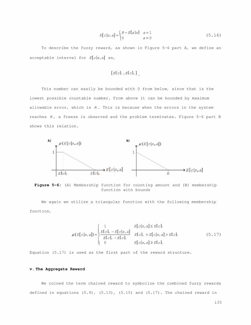
[ ][ ] 1
,0 0R E s a
E c s aa
ε− == = (5.16)
To describe the fuzzy reward, as shown in Figure 5-6 part A, we define an
acceptable interval for [ ],E c s a as,
[ ] [ ][ ],l uE c E c .
This number can easily be bounded with 0 from below, since that is the
lowest possible countable number. From above it can be bounded by maximum
allowable error, which is R . This is because when the errors in the system
reaches R , a freeze is observed and the problem terminates. Figure 5-6 part B
shows this relation.
Figure 5-6: (A) Membership function for counting amount and (B) membership function with bounds
We again we utilize a triangular function with the following membership
function,
[ ]( )
[ ] [ ][ ] [ ][ ] [ ]
[ ] [ ] [ ]
[ ] [ ]
1 , ,
, ,
0 ,
l
uu l
u l
u
E c s a E cE c E c s a
E c s a E c E c s a E cE c E c
E c s a E c
µ
≤ −
= > >−
≥
(5.17)
Equation (5.17) is used as the first part of the reward structure.
v. The Aggregate Reward
We coined the term chained reward to symbolize the combined fuzzy rewards
defined in equations (5.9), (5.13), (5.15) and (5.17). The chained reward in
135
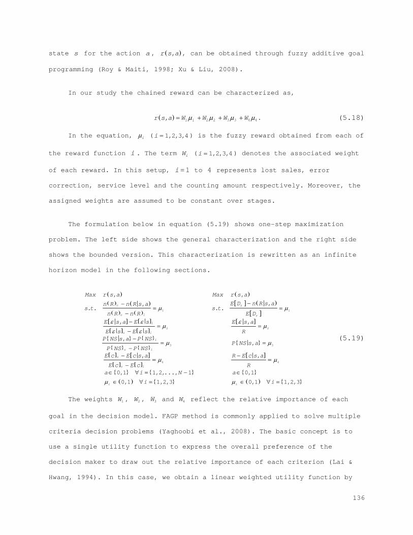
state s for the action a , ( ),r s a , can be obtained through fuzzy additive goal
programming (Roy & Maiti, 1998; Xu & Liu, 2008).
In our study the chained reward can be characterized as,
( ) 1 1 2 2 3 3 4 4,r s a W W W Wµ µ µ µ= + + + . (5.18)
In the equation, iµ ( 1,2,3,4i = ) is the fuzzy reward obtained from each of
the reward function i . The term iW ( 1,2,3,4i = ) denotes the associated weight
of each reward. In this setup, 1i = to 4 represents lost sales, error
correction, service level and the counting amount respectively. Moreover, the
assigned weights are assumed to be constant over stages.
The formulation below in equation (5.19) shows one-step maximization
problem. The left side shows the general characterization and the right side
shows the bounded version. This characterization is rewritten as an infinite
horizon model in the following sections.
( ) ( )( ) ( )( ) ( )
[ ] ( )
[ ][ ] [ ]
[ ] [ ]
[ ]
{ } { }
{ } { }{ }
[ ] [ ][ ]
1 1
2 2
3 3
, ,
,,. . . .
, ,
, ,
,
u
u l
l
u l
l
u l
u
u
Max r s a Max r s a
E D n R s an R n R s as t s t
n R n R E DE s a E s E s a
E s E s RP NS s a P NS
P NS s aP NS P NSE c E c s a
E c
τ
τ
µ µ
ε ε εµ µ
ε ε
µ µ
−−= =
−−
= =−−
= =−
−[ ]
[ ]
{ } { } { }
( ) { } ( ) { }
4 4
,
0,1 1,2,..., 1 0,1
0,1 1,2,3 0,1 1,2,3
l
i i
R E c s a
E c Ra i N a
i i
µ µ
µ µ
−
−∈ ∀ = − ∈
∈ ∀ = ∈ ∀ =
= =
(5.19)
The weights 1W , 2W , 3W and 4W reflect the relative importance of each
goal in the decision model. FAGP method is commonly applied to solve multiple
criteria decision problems (Yaghoobi et al., 2008). The basic concept is to
use a single utility function to express the overall preference of the
decision maker to draw out the relative importance of each criterion (Lai &
Hwang, 1994). In this case, we obtain a linear weighted utility function by
136
multiplying each membership function of fuzzy goals with their corresponding
weights and then adding the results together. The weighted additive model,
proposed by Tiwari et al. (1987), belongs to the convex fuzzy models outlined
by Bellman and Zadeh (1970). One important shortcoming of additive models is
that the weights are assumed to be known. In reality this is not always
correct; hence, we conducted sensitivity analysis on various weights to study
the influence of the weights and the effect of error.
5.1.5 Infinite-Horizon Discounted MDP
Optimizing sequential decision making problems requires the computation
of objective function for each combination of values. This becomes a
significant obstacle when the dimension of the state variable is large. As
pointed out by Rust (1997) this can considerably reduce the ability to solve
continuous MDPs accurately. In literature such problems are often referred as
the curse of dimensionality (Bellman, 1957; Bellman & Dreyfus, 1962).
In this study we model an infinite-horizon discrete-time discounted MDP.
In our problem the state space is the difference of two data sources (records
and visibility), which are both fully observable. At each decision epoch
decision maker has two alternatives; cycle counting or not. The immediate
rewards obtained after the actions are bounded and stationary. The transition
probabilities do not change over time and the state space is finite.
By using the expected total discounted reward as the objective function
we solve our problem using policy iteration algorithm. The policy iteration
algorithm, as described in Puterman (2009), first selects an arbitrary policy
and then calculates the corresponding value function. Then, one by one
different policies are generated and corresponding value functions are
compared iteratively. At the end of each iteration, the generated policies
137
are either updated or discarded based on the value function comparison. This
cycle continues until no improvement is possible.
Let ( )v sπλ represent the expected total discounted reward of policy π ,
where 0 1λ≤ ≤ . Then infinite-horizon optimality equations can be formed as
( ) ( ) ( ) ( )sup , ,a A s S
v s r s a P s s a v sπ πλ λλ
∈ ′∈
′ ′= +
∑
see (Puterman, 2009).
5.2 Structural Properties
In this section, we examine the sufficient conditions that ensure the
existence of an optimal control limit policy. The control limit type policy
in MDP framework can be briefly explained as follows: The optimal decision
rule is to trigger a cycle count when the current state is above a threshold
state *s and do nothing if it is below *s . In other words, the cycle count is
done if and only if the observed state is among * *, 1,..., 1s s R+ + (Barlow &
Proschan, 1996). In this paper we refer this type as threshold type policy.
Also, it is widely known that when the optimal policy is of threshold type
the problem typically can be solved more efficiently, as demonstrated in
Puterman (2009).
Below, we discuss some observations that are used to specify special
structures about the optimal policy. Interested readers should refer to
(Barlow & Proschan, 1996; Puterman, 2009).
5.2.1 Transition Matrix
Property 1: ( ),q k s a is non-decreasing in s for all a , where
138
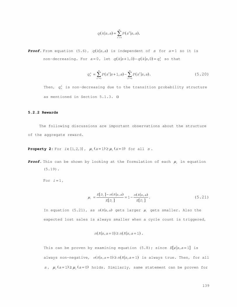
( ) ( ), , .s k
q k s a P s s a∞
′=
′= ∑
Proof. From equation (5.6), ( ),q k s a is independent of s for 1a = so it is
non-decreasing. For 0a = , let ( ) ( )1,0 ,0 ksq k s q k s q+ − = so that
( ) ( )1, ,ks
s k s k
q P s s a P s s a∞ ∞
′ ′= =
′ ′= + −∑ ∑ . (5.20)
Then, ksq is non-decreasing due to the transition probability structure
as mentioned in Section 5.1.3.
5.2.2 Rewards
The following discussions are important observations about the structure
of the aggregate reward.
Property 2: For { }1,2,3i∈ , ( ) ( )1 0i ia aµ µ= ≥ = for all s .
Proof. This can be shown by looking at the formulation of each iµ in equation
(5.19).
For 1i = ,
[ ] ( )
[ ]( )
[ ]1
, ,1
E D n R s a n R s a
E D E D
τ
τ τ
µ−
= = − . (5.21)
In equation (5.21), as ( ),n R s a gets larger 1µ gets smaller. Also the
expected lost sales is always smaller when a cycle count is triggered,
( ) ( ), 0 , 1n R s a n R s a= ≥ = .
This can be proven by examining equation (5.8); since [ ], 1E s aε = is
always non-negative, ( ) ( ), 0 , 1n R s a n R s a= ≥ = is always true. Then, for all
s , ( ) ( )1 11 0a aµ µ= ≥ = holds. Similarly, same statement can be proven for
139
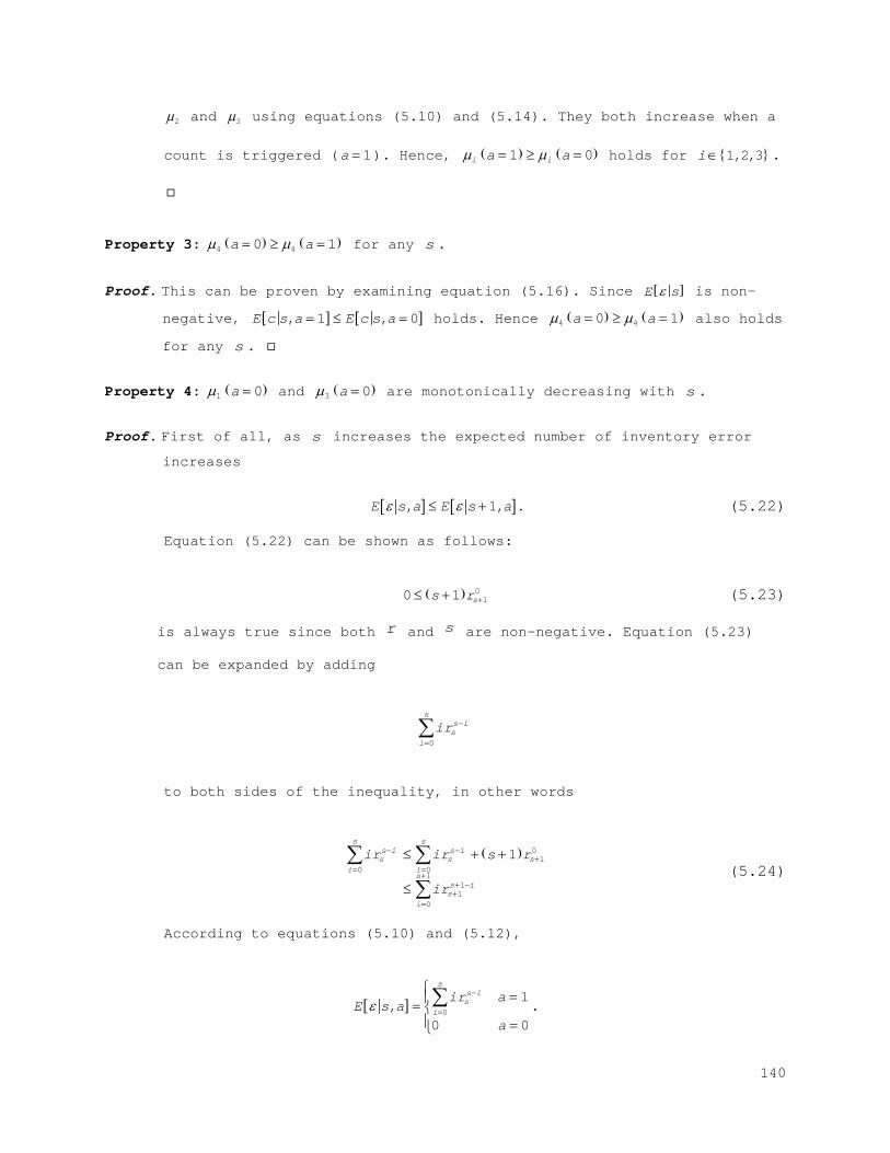
2µ and 3µ using equations (5.10) and (5.14). They both increase when a
count is triggered ( 1a = ). Hence, ( ) ( )1 0i ia aµ µ= ≥ = holds for { }1,2,3i∈ .
Property 3: ( ) ( )4 40 1a aµ µ= ≥ = for any s .
Proof. This can be proven by examining equation (5.16). Since [ ]E sε is non-
negative, [ ] [ ], 1 , 0E c s a E c s a= ≤ = holds. Hence ( ) ( )4 40 1a aµ µ= ≥ = also holds
for any s .
Property 4: ( )1 0aµ = and ( )
3 0aµ = are monotonically decreasing with s .
Proof. First of all, as s increases the expected number of inventory error increases
[ ] [ ], 1,E s a E s aε ε≤ + . (5.22)
Equation (5.22) can be shown as follows:
( ) 010 1 ss r +≤ + (5.23)
is always true since both r and s are non-negative. Equation (5.23)
can be expanded by adding
0
ss is
i
ir −
=∑
to both sides of the inequality, in other words
( ) 0
10 0
111
0
1s s
s i s is s s
i is
s is
i
ir ir s r
ir
− −+
= =+
+ −+
=
≤ + +
≤
∑ ∑
∑ (5.24)
According to equations (5.10) and (5.12),
[ ] 0
1,
0 0
ss is
i
ir aE s a
aε
−
=
== =
∑ .
140
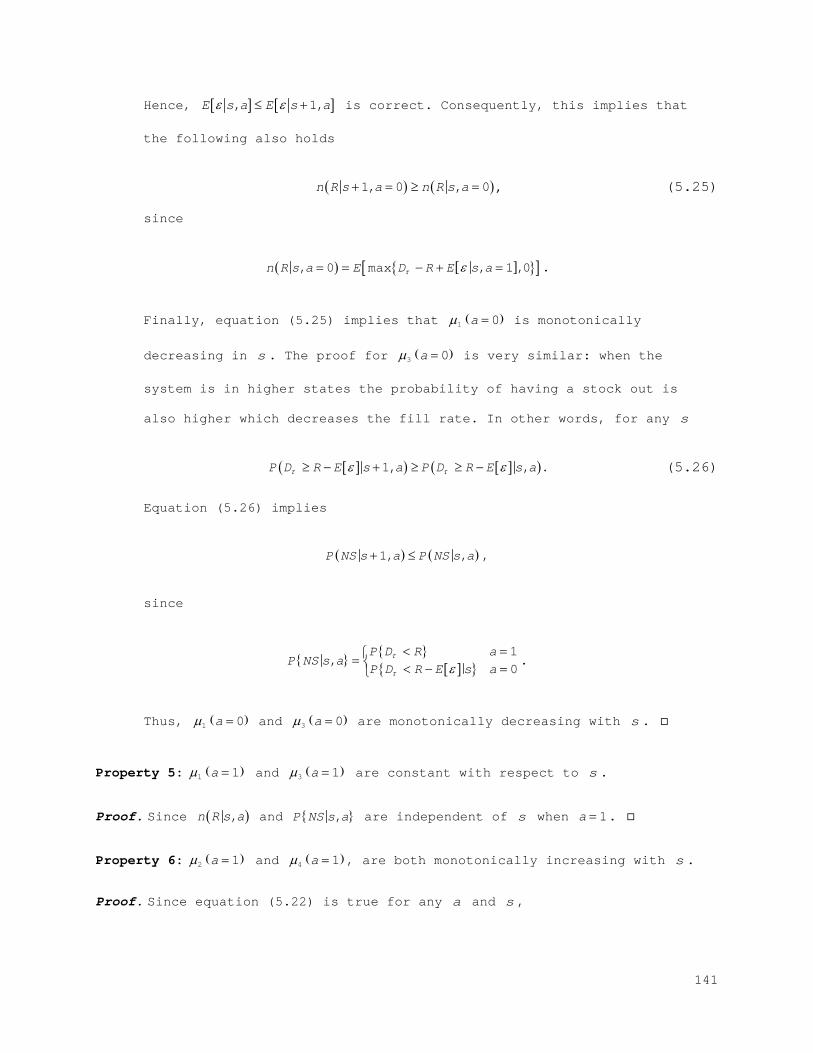
Hence, [ ] [ ], 1,E s a E s aε ε≤ + is correct. Consequently, this implies that
the following also holds
( ) ( )1, 0 , 0n R s a n R s a+ = ≥ = , (5.25)
since
( ) [ ]{ }[ ], 0 max , 1 ,0n R s a E D R E s aτ ε= = − + = .
Finally, equation (5.25) implies that ( )1 0aµ = is monotonically
decreasing in s . The proof for ( )3 0aµ = is very similar: when the
system is in higher states the probability of having a stock out is
also higher which decreases the fill rate. In other words, for any s
[ ]( ) [ ]( )1, ,P D R E s a P D R E s aτ τε ε≥ − + ≥ ≥ − . (5.26)
Equation (5.26) implies
( ) ( )1, ,P NS s a P NS s a+ ≤ ,
since
{ } { }[ ]{ }
1,
0P D R a
P NS s aP D R E s a
τ
τ ε< == < − =
.
Thus, ( )1 0aµ = and ( )
3 0aµ = are monotonically decreasing with s .
Property 5: ( )1 1aµ = and ( )
3 1aµ = are constant with respect to s .
Proof. Since ( ),n R s a and { },P NS s a are independent of s when 1a = .
Property 6: ( )2 1aµ = and ( )
4 1aµ = , are both monotonically increasing with s .
Proof. Since equation (5.22) is true for any a and s ,
141
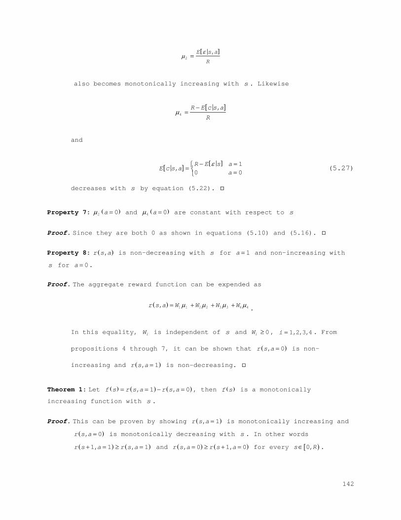
[ ]2
,E s a
R
εµ =
also becomes monotonically increasing with s . Likewise
[ ]4
,R E c s a
Rµ
−=
and
[ ][ ] 1
,0 0R E s a
E c s aa
ε− == = (5.27)
decreases with s by equation (5.22).
Property 7: ( )2 0aµ = and ( )
4 0aµ = are constant with respect to s
Proof. Since they are both 0 as shown in equations (5.10) and (5.16).
Property 8: ( ),r s a is non-decreasing with s for 1a = and non-increasing with
s for 0a = .
Proof. The aggregate reward function can be expended as
( ) 1 1 2 2 3 3 4 4,r s a W W W Wµ µ µ µ= + + + .
In this equality, iW is independent of s and 0iW ≥ , 1,2,3,4i = . From
propositions 4 through 7, it can be shown that ( ), 0r s a = is non-
increasing and ( ), 1r s a = is non-decreasing.
Theorem 1: Let ( ) ( ) ( ), 1 , 0f s r s a r s a= = − = , then ( )f s is a monotonically
increasing function with s .
Proof. This can be proven by showing ( ), 1r s a = is monotonically increasing and
( ), 0r s a = is monotonically decreasing with s . In other words
( ) ( )1, 1 , 1r s a r s a+ = ≥ = and ( ) ( ), 0 1, 0r s a r s a= ≥ + = for every [ )0,s R∈ .
142
For s S∈ and { }1,2,3,4i∈ , ( ), 1r s a = is a convex combination of ( )1i aµ =
and ( ), 0r s a = is a convex combination of ( )0i aµ = where [ ]0,1iW ∈ and
4
1
1ii
W=
=∑ ,
as shown in (5.18). Since ( )1 0aµ = , ( )
3 0aµ = are monotonically decreasing
and ( )2 0aµ = , ( )
4 0aµ = are constant with s . Any convex combination of
them is also monotonically decreasing with s . Similarly, ( )1 1aµ = ,
( )3 1aµ = are constant and ( )
2 1aµ = , ( )4 1aµ = are monotonically increasing
with s . Any convex combination of them is also monotonically increasing
with s . Hence, ( )f s is monotonically increasing with s .
5.2.3 Value Function and Policy
According to Puterman (2009) under following conditions:
1. Stationary rewards and transition probabilities: ( ),r s a and ( ),P s s a′
do not change from decision epoch to decision epoch.
2. Bounded rewards: ( ),r s a M≤ < ∞ for all a and s .
3. Discounting: future rewards are discounted according to discount
factor λ , with 0 1λ≤ < .
4. Discrete state space; S is finite and countable.
Theorem 2: For any stationary policy π , there is a unique solution vπλ .
Theorem 3: A policy *π optimal if and only if *
vπλ is a solution of the
optimality equation.
143
Theorem 4: For a discrete S if sA is compact, ( ),r s a is continuous for each s
and ( ),P s s a′ is continuous in a for each s and s ′ . Then there exists an
optimal deterministic stationary policy.
Proof. See Puterman (2009) for theorems 2 through 4.
Theorem 5: The structure of the optimal policy is a control limit type as long
as assumptions 1 through 4 are satisfied and [ ]0,1iW ∈ for every i ,
4
1
1ii
W=
=∑ .
Proof. Assume that there exists an *s such that ( ) 0d s = for all *s s< and
( ) 1d s = for all *s s≥ . This assumption implies that for every *s s<
( ) ( ) ( ) ( ) ( ) ( )1 1
0 0
,1 ,1 ,0 ,0R R
s s
r s P s s v s r s P s s v sλ λ+ +
′ ′= =
′ ′ ′ ′+ ≤ +∑ ∑
and for every *s s≥
( ) ( ) ( ) ( ) ( ) ( )1 1
0 0
,1 ,1 ,0 ,0R R
s s
r s P s s v s r s P s s v sλ λ+ +
′ ′= =
′ ′ ′ ′+ ≥ +∑ ∑ .
Let’s assume the converse of the assumption is true. In other words,
there exists an *s s< such that ( ) 0d s = and ( )1 1d s − = . This can be
formulated as
( ) ( ) ( ) ( ) ( ) ( )1 1
0 0
,1 ,1 ,0 ,0R R
s s
r s P s s v s r s P s s v sλ λ+ +
′ ′= =
′ ′ ′ ′+ ≤ +∑ ∑ (5.28)
and
( ) ( ) ( ) ( ) ( ) ( )1 1
0 0
1,1 1,1 1,0 1,0R R
s s
r s P s s v s r s P s s v sλ λ+ +
′ ′= =
′ ′ ′ ′− + − > − + −∑ ∑ . (5.29)
Equations (5.28) and (5.29) can be respectively rewritten as
144
( ) ( ) ( ) ( ) ( )( )1
0
,1 ,0 ,0 ,1R
s
r s r s v s P s s P s sλ+
′=
′ ′ ′− ≤ − ∑ (5.30)
and
( ) ( ) ( ) ( ) ( )( )1
0
1,1 1,0 1,0 1,1R
s
r s r s v s P s s P s sλ+
′=
′ ′ ′− − − > − − − ∑ (5.31)
In property 9 it is already proven that ( ) ( ) ( ),1 ,0f s r s r s= − is a
monotonically increasing function in terms of s . This implies that
( ) ( )1 0f s f s− − ≤ . Then, by subtracting equation (5.30) from equation
(5.31) we get
( ) ( )( ) ( ) ( )( )
( ) ( ) ( )( )
( ) ( ) ( )( )
( ) ( ) ( )( )
1
01
01
01
0
1,0 1,11
,0 ,1
1,0 1,10
,0 ,1
R
sR
sR
sR
s
v s P s s P s sf s f s
v s P s s P s s
v s P s s P s s
v s P s s P s s
λ
λ
+
′=+
′=+
′=+
′=
′ ′ ′− − − − − >
′ ′ ′− − ′ ′ ′− − −
> ′ ′ ′− −
∑
∑
∑
∑
(5.32)
In equation (5.32), λ is a non-negative number between 0 and 1;
removing it does not violate the inequality. Also, by definition
( ) ( ),1 0,0P s s P s′ ′= for any s , so we can rewrite the equation as
( ) ( ) ( ) ( ) ( )( )[ ]1
0
0 1,0 0,0 ,0 0,0 .R
s
v s P s s P s P s s P s+
′=
′ ′ ′ ′ ′> − − − +∑ (5.33)
Subsequently, it can be simplified as
( ) ( ) ( ) ( )( )1 1
0 0
,0 1,0R R
s s
v s P s s v s P s s+ +
′ ′= =
′ ′ ′ ′> −∑ ∑ (5.34)
where both ( )v s ′ and ( ),0P s s′ are non-negative for any s . Hence,
equation (5.34) is equivalent to saying ( ) ( )( ),0 1,0P s s P s s′ ′> − for all
*s s< . This is simply not true for every possible realization. Which
means there exists a contradiction, meaning ( )* 0d s = implies ( )* 1 0d s − =
for *s s< .
145
Similarly, ( ) 1d s = for *s s≥ can easily be proven by employing the same
logic. Hence, ( )* 0d s = implies ( )* 1 0d s − = for *s s< and ( )* 1d s = implies
( )* 1 1d s + = for *s s≥ . Meaning the optimal policy is a threshold type.
5.3 Numerical Analysis
To demonstrate the performance of our algorithm we solved the same case
study provided in previous chapters. Recall, in the case study a ( ),Q R policy
is utilized with ( )600,80 . The weekly demand is normally distributed with
( )250,12 and lead time is also normally distributed with ( )21.14,0.33 .
Furthermore, by utilizing the error characterization provided in chapter 3 we
used normal distribution with ( )23.83,7.17 for errors. We compare three level
visibility performance with truncated normal distribution.
As mentioned the mean is set to zero to ensure that the system is not
intentionally making errors. The standard deviation however, depends on the
current state and it is the factor that defines the performance. Intuitively,
in an ideal setup the unbiased visibility yields ( )0 1P sε = = if t is zero and
( ) 0P t sε = = if 0t > ; this is a matrix with ones in column zero and zeroes
everywhere else. Similarly the worst unbiased visibility would assume a
uniform shape across t. In other words, in such a scenario ( ) 1/P t s sε = = for
every t and s . In reality the visibility performance will behave somewhere
in between these two extremes.
5.3.1 Transition Matrix
In our example, ( )P t sε = follows a truncated normal distribution with
mean zero and variance εσ . If εσ is zero, then the visibility will be perfect
146
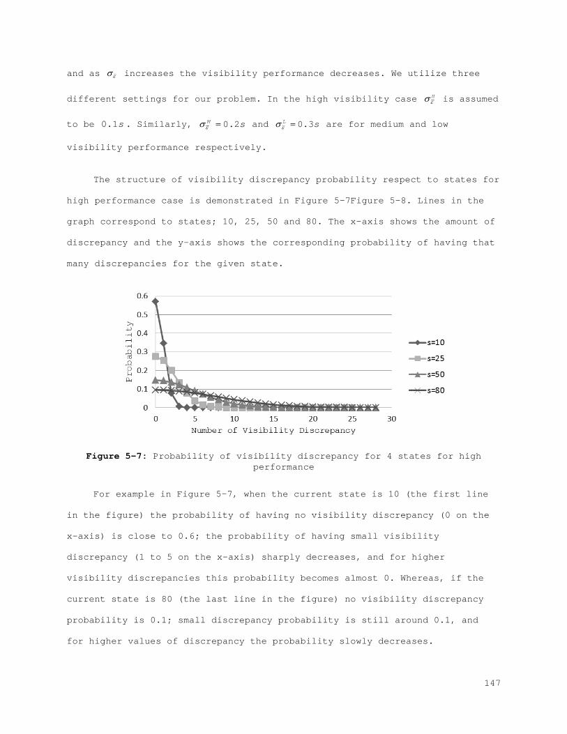
and as εσ increases the visibility performance decreases. We utilize three
different settings for our problem. In the high visibility case Hεσ is assumed
to be 0.1s . Similarly, 0.2M sεσ = and 0.3L sεσ = are for medium and low
visibility performance respectively.
The structure of visibility discrepancy probability respect to states for
high performance case is demonstrated in Figure 5-7Figure 5-8. Lines in the
graph correspond to states; 10, 25, 50 and 80. The x-axis shows the amount of
discrepancy and the y-axis shows the corresponding probability of having that
many discrepancies for the given state.
Figure 5-7: Probability of visibility discrepancy for 4 states for high performance
For example in Figure 5-7, when the current state is 10 (the first line
in the figure) the probability of having no visibility discrepancy (0 on the
x-axis) is close to 0.6; the probability of having small visibility
discrepancy (1 to 5 on the x-axis) sharply decreases, and for higher
visibility discrepancies this probability becomes almost 0. Whereas, if the
current state is 80 (the last line in the figure) no visibility discrepancy
probability is 0.1; small discrepancy probability is still around 0.1, and
for higher values of discrepancy the probability slowly decreases.
147
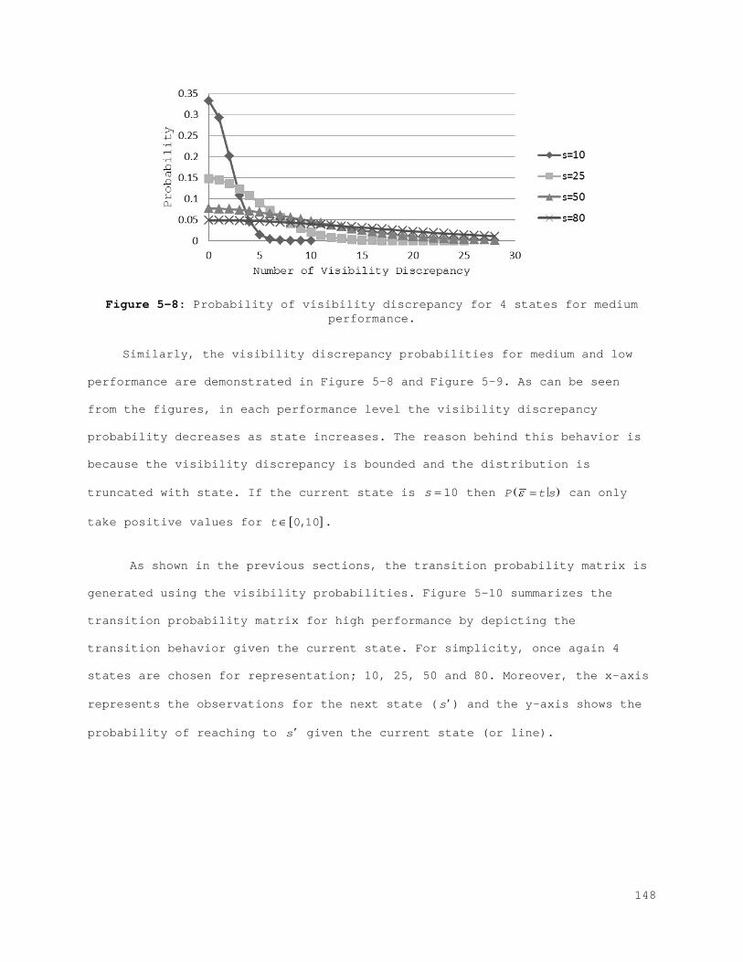
Figure 5-8: Probability of visibility discrepancy for 4 states for medium performance.
Similarly, the visibility discrepancy probabilities for medium and low
performance are demonstrated in Figure 5-8 and Figure 5-9. As can be seen
from the figures, in each performance level the visibility discrepancy
probability decreases as state increases. The reason behind this behavior is
because the visibility discrepancy is bounded and the distribution is
truncated with state. If the current state is 10s = then ( )P t sε = can only
take positive values for [ ]0,10t∈ .
As shown in the previous sections, the transition probability matrix is
generated using the visibility probabilities. Figure 5-10 summarizes the
transition probability matrix for high performance by depicting the
transition behavior given the current state. For simplicity, once again 4
states are chosen for representation; 10, 25, 50 and 80. Moreover, the x-axis
represents the observations for the next state (s ′) and the y-axis shows the
probability of reaching to s ′ given the current state (or line).
148
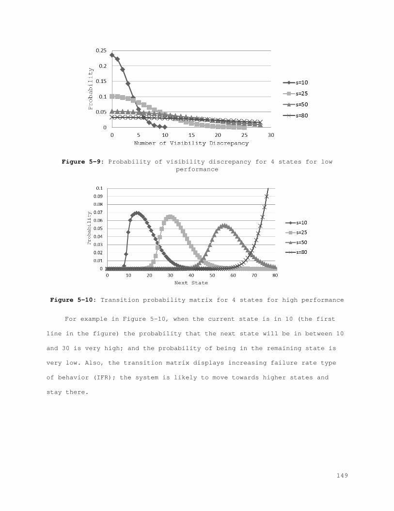
Figure 5-9: Probability of visibility discrepancy for 4 states for low performance
Figure 5-10: Transition probability matrix for 4 states for high performance
For example in Figure 5-10, when the current state is in 10 (the first
line in the figure) the probability that the next state will be in between 10
and 30 is very high; and the probability of being in the remaining state is
very low. Also, the transition matrix displays increasing failure rate type
of behavior (IFR); the system is likely to move towards higher states and
stay there.
149
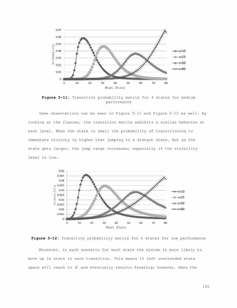
Figure 5-11: Transition probability matrix for 4 states for medium performance
Same observations can be seen in Figure 5-11 and Figure 5-12 as well. By
looking at the figures, the transition matrix exhibits a similar behavior at
each level. When the state is small the probability of transitioning to
immediate vicinity is higher than jumping to a distant state. But as the
state gets larger, the jump range increases; especially if the visibility
level is low.
Figure 5-12: Transition probability matrix for 4 states for low performance
Moreover, in each scenario for each state the system is more likely to
move up in state in each transition. This means if left unattended state
space will reach to R and eventually results freezing; however, when the
150
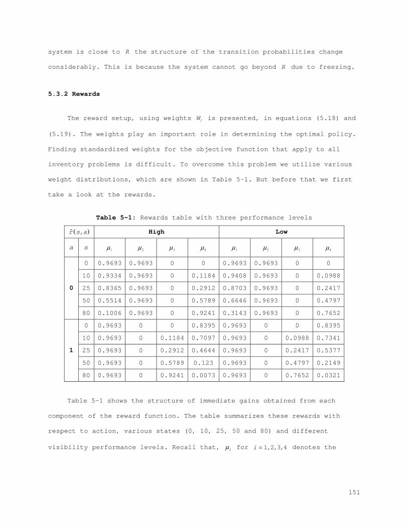
system is close to R the structure of the transition probabilities change
considerably. This is because the system cannot go beyond R due to freezing.
5.3.2 Rewards
The reward setup, using weights iW is presented, in equations (5.18) and
(5.19). The weights play an important role in determining the optimal policy.
Finding standardized weights for the objective function that apply to all
inventory problems is difficult. To overcome this problem we utilize various
weight distributions, which are shown in Table 5-1. But before that we first
take a look at the rewards.
Table 5-1: Rewards table with three performance levels
( ),r s a High Low
a s 1µ 2µ 3µ 4µ 1µ 2µ 3µ 4µ
0
0 0.9693 0.9693 0 0 0.9693 0.9693 0 0
10 0.9334 0.9693 0 0.1184 0.9408 0.9693 0 0.0988
25 0.8365 0.9693 0 0.2912 0.8703 0.9693 0 0.2417
50 0.5514 0.9693 0 0.5789 0.6646 0.9693 0 0.4797
80 0.1006 0.9693 0 0.9241 0.3143 0.9693 0 0.7652
1
0 0.9693 0 0 0.8395 0.9693 0 0 0.8395
10 0.9693 0 0.1184 0.7097 0.9693 0 0.0988 0.7341
25 0.9693 0 0.2912 0.4644 0.9693 0 0.2417 0.5377
50 0.9693 0 0.5789 0.123 0.9693 0 0.4797 0.2149
80 0.9693 0 0.9241 0.0073 0.9693 0 0.7652 0.0321
Table 5-1 shows the structure of immediate gains obtained from each
component of the reward function. The table summarizes these rewards with
respect to action, various states (0, 10, 25, 50 and 80) and different
visibility performance levels. Recall that, iµ for 1,2,3,4i = denotes the
151
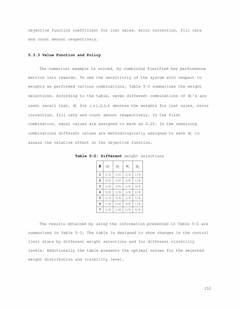
objective function coefficient for lost sales, error correction, fill rate
and count amount respectively.
5.3.3 Value Function and Policy
The numerical example is solved, by combining fuzzified key performance
metrics into rewards. To see the sensitivity of the system with respect to
weights we performed various combinations. Table 5-2 summarizes the weight
selections. According to the table, seven different combinations of iW ’s are
used; recall that, iW for 1,2,3,4i = denotes the weights for lost sales, error
correction, fill rate and count amount respectively. In the first
combination, equal values are assigned to each as 0.25. In the remaining
combinations different values are methodologically assigned to each iW to
assess the relative effect on the objective function.
Table 5-2: Different weight selections
# 1W 2W 3W 4W
1 1/4 1/4 1/4 1/4
2 3/8 1/8 3/8 1/8
3 1/8 3/8 1/8 3/8
4 5/8 1/8 1/8 1/8
5 1/8 5/8 1/8 1/8
6 1/8 1/8 5/8 1/8
7 1/8 1/8 1/8 5/8
The results obtained by using the information presented in Table 5-2 are
summarized in Table 5-3. The table is designed to show changes in the control
limit state by different weight selections and for different visibility
levels. Additionally the table presents the optimal values for the selected
weight distribution and visibility level.
152
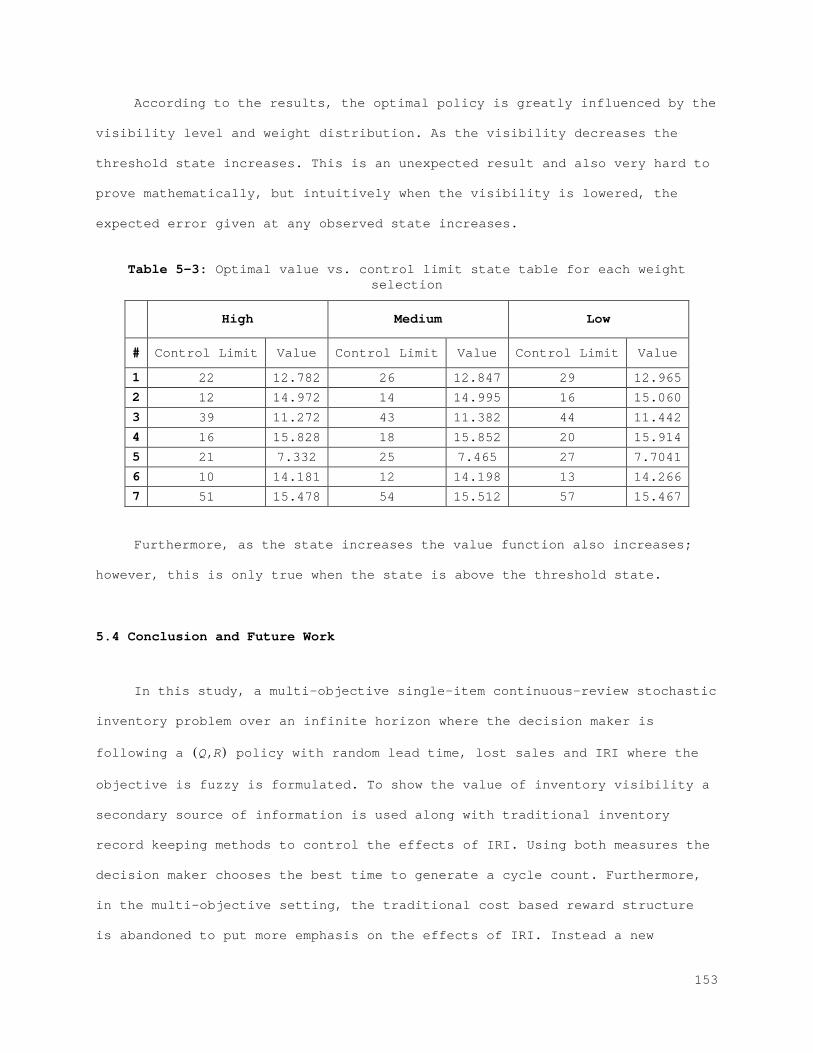
According to the results, the optimal policy is greatly influenced by the
visibility level and weight distribution. As the visibility decreases the
threshold state increases. This is an unexpected result and also very hard to
prove mathematically, but intuitively when the visibility is lowered, the
expected error given at any observed state increases.
Table 5-3: Optimal value vs. control limit state table for each weight selection
High Medium Low
# Control Limit Value Control Limit Value Control Limit Value
1 22 12.782 26 12.847 29 12.965
2 12 14.972 14 14.995 16 15.060
3 39 11.272 43 11.382 44 11.442
4 16 15.828 18 15.852 20 15.914
5 21 7.332 25 7.465 27 7.7041
6 10 14.181 12 14.198 13 14.266
7 51 15.478 54 15.512 57 15.467
Furthermore, as the state increases the value function also increases;
however, this is only true when the state is above the threshold state.
5.4 Conclusion and Future Work
In this study, a multi-objective single-item continuous-review stochastic
inventory problem over an infinite horizon where the decision maker is
following a ( ),Q R policy with random lead time, lost sales and IRI where the
objective is fuzzy is formulated. To show the value of inventory visibility a
secondary source of information is used along with traditional inventory
record keeping methods to control the effects of IRI. Using both measures the
decision maker chooses the best time to generate a cycle count. Furthermore,
in the multi-objective setting, the traditional cost based reward structure
is abandoned to put more emphasis on the effects of IRI. Instead a new
153
measure is developed as inventory performance by combining four key
performance metrics; lost sales, amount of correction, fill rate and amount
of inventory counted. These key metrics are combined under a unitless
platform using fuzzy logic and combined through additive methods.
The inventory problem is modeled as an infinite horizon discounted MDP
with fuzzified multi-objective. The optimal policy is shown to be a control
limit policy. Finally, the results are shown in a brief numerical example
solved by policy iteration algorithm.
The dynamic programming model in this chapter is designed to find the
optimal inventory performance using the error correction and control method.
This model can be extended by implementing the IRI resistance method. In that
case, the decision maker has two decision available at each decision epoch,
whether to do a cycle count or not and to decide on the best increment level.
154
REFERENCES
Agrawal, V. (2001). Assessing the Benefits of Auto-ID Technology in the Consumer Goods Industry. MIT, Technical Report of the Auto ID Center.
Barlow, R. E., & Proschan, F. (1996). Mathematical theory of reliability:
(No. 17) Siam. Bashyam, S., & Fu, M. C. (1998). Optimization of (s, S) inventory systems
with random lead times and a service level constraint. Management Science, s243-s256.
Bellman, R. E. (1957). A Markovian decision process: DTIC Document. Bellman, R. E., & Dreyfus, S. E. (1962). Applied dynamic programming. Bellman, R. E., & Zadeh, L. A. (1970). Decision-making in a fuzzy
environment. Management Science, 17, 141-164. Chang, H. C., Yao, J. S., & Ouyang, L. Y. (2006). Fuzzy mixture inventory
model involving fuzzy random variable lead time demand and fuzzy total demand. European Journal of Operational Research, 169, 165-180.
Chen, L. H., & Tsai, F. C. (2001). Fuzzy goal programming with different
importance and priorities. European Journal of Opertaional Research, 133, 348-556.
Chen, S. P. (2011). A membership function approach to lot size re-order point
inventory problems in fuzzy environments. International Journal of Production Reserach, 49, 3855-3871.
Dutta, P., Chakraborty, D., & Roy, A. R. (2007). Continuous review inventory
model in mixed fuzzy and stochastic environment. Applied Mathematics and Computation, 188, 970-980.
Gumrukcu, S., Rossetti, M. D., & Buyurgan, N. (2008). Quantifying the costs
of cycle counting in a two-echelon supply chain with multiple items. International Journal of Production Economics, 116, 263-274.
Kiefer, A. W., & Novack, R. A. (1999). An empirical analysis of warehouse
measurement systems in the context of supply chain implementation. Transportation Journal, 38, 18-27.
Kosko, B. (1992). Neural networks and fuzzy systems.: Prentice hall. Lai, Y.-J., & Hwang, C.-L. (1994). Fuzzy multiple objective decision making:
Springer. Lin, Y. J. (2008). A periodic review inventory model involving fuzzy expected
demand short and fuzzy backorder rate. Computers & Industrial Engineering, 54, 666-676.
Ouyang, L. Y., & Chang, H. C. (2002). A minimax distribution free procedure
for mixed inventory models involving variable lead time with fuzzylost sales. Int. J. Production Economics, 76,71-12.
155
Ouyang, L. Y., & Wu, K. S. (1997). Mixture inventory model involving variable lead time with a service level constraint. Computers & operations research, 24, 875-882.
Puterman, M. L. (2009). Markov decision processes: discrete stochastic
dynamic programming. New Jersey: John Wiley & Sons. Raman, A., Dehoratius, N., & Ton, Z. (2001, Spring). Execution: The missing
link in retail operations. California Management Review, 43, 136-152. Rosenthal, R. E. (1985). Concepts theory and techniques: Principles of multi-
objective optimization. Decision Sciences, 16, 133-152. Roy, T. K., & Maiti, M. (1998). Multi-objective inventory models of
deteriorating items with some constraints in a fuzzy environment. Computers & operations research, 25, 1085-1095.
Rust, J. (1997). Using randomization to break the curse of dimensionality.
Econometrica: Journal of the Econometric Society, 487-516. Stevenson, W. J., & Hojati, M. (2007). Operations management. Boston: McGraw-
Hill/Irwin. Tarim, S. A., & Kingsman, B. G. (2004). The stochastic dynamic
production/inventory lot-sizing problem with service-level constraints. nternational Journal of Production Economics, 88, 105-119.
Thiel, D., Hovelaque, V., & Hoa, V. T. L. (2010). Impact of inventory
inaccuracy on service-leve lquality in (Q,R) continuous-review lost-sales inventory models. Int. J. Production Economics, 123, 301-311.
Tiwari, R., Dharmar, S., & Rao, J. (1987). Fuzzy goal programming—an additive
model. Fuzzy sets and systems, 24(1), 27-34. Ton, Z., & Raman, A. (2004). An empirical anaylsis of misplaced skus in
reatil stores. Harvard Business School. Vujosevic, M., Petrovic, D., & Petrovic, R. (1996). EOQ formula when
inventory cost is fuzzy. International Journal of Production Economics, 45, 499-504.
Wee, H. M., Lo, C. C., & Hsu, P. H. (2009). A multi-objective joint
replenishment inventory model of deteriorated items in a fuzzy environment. European Journal of Operational Research, 197, 620-631.
Xexéo, G. Fuzzy Logic. Federal University of Rio de Janeiro: Computing
Science Department and Systems and Computing. Engineering Program. Xu, J., & Liu, Y. (2008). Multi-objective decision making model under fuzzy
random environment and its application to invenotry problems. Information Sciences, 178, 2899-2914.
Yaghoobi, M. A., Jones, D. F., & Tamiz, M. (2008). Weighted additive models
for solving fuzzy goal programming problems. Asia-Pacific Journal of Operational Research, 25, 715.
156
Yao, J. S., & Chiang, J. (2003). Inventory without backorder with fuzzy total cost and fuzzy storing cost defuzzified by centroid and signed distance. European Journal of Operational Research, 148, 401-409.
Zadeh, L. A. (1965). Fuzzy sets. Information and control, 8,338-353. Zimmermann, H. J. (1978). Fuzzy programming and linear programming with
several objective functions. Fuzzy Set and Systems, 1, 45-55. Zipkin, P. H. (2000). Foundations of inventory management. New York: McGraw-
Hill.
157
CHAPTER 6 CONCLUSION
Supply chain and inventory management has always been a major concern in
the business world as well as in the academic domain. The scope entails
physical holding, lead times, holding costs, replenishment, defective goods,
quality control, transportation, storage, and inventory visibility. Hence,
inventory models can be regarded as one of the most widely studied topics in
industrial engineering and operations management. The main goal for most of
these studies is to reach efficient solutions that would provide cost
effective realizations in practice. Due to the uncertain nature of the world,
these models are known to have a complex structure. In practice, dealing with
all the uncertain factors, satisfying the high service levels and reaching
optimal solutions at the same time is challenging. Starting from late 70s,
theoretical studies began addressing the difficulties faced in inventory
management. In industries where the competition is fierce and profit margins
are thin, companies have automated the inventory management processes to
better meet customer demand and reduce operational costs. Such schemes
significantly decreased the response time of the decision makers, making it
dramatically easy to keep track of the records and avoid human intervention
as much as possible. However, the automation of management processes
transferred the entire critical decision making - such as what products are
where and in what quantity - from humans to computers. As a result
understanding the value of data accuracy and controlling the impact of data
inaccuracy became a crucial part of inventory management problems. The aims
to answer the following two questions: What is the impact of IRI? And how
can we control IRI?
158
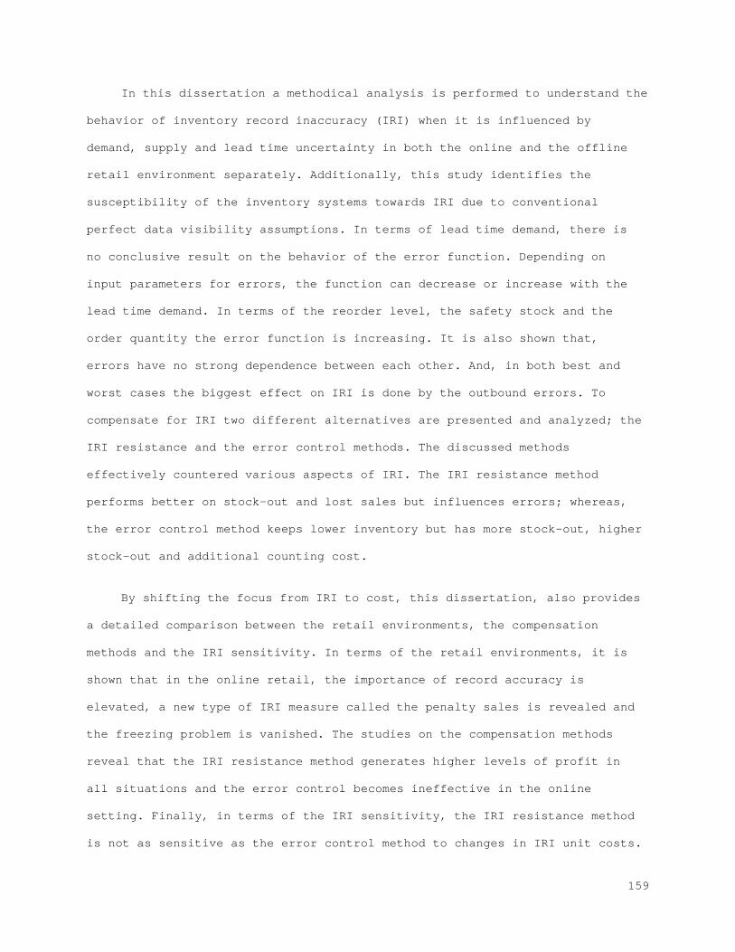
In this dissertation a methodical analysis is performed to understand the
behavior of inventory record inaccuracy (IRI) when it is influenced by
demand, supply and lead time uncertainty in both the online and the offline
retail environment separately. Additionally, this study identifies the
susceptibility of the inventory systems towards IRI due to conventional
perfect data visibility assumptions. In terms of lead time demand, there is
no conclusive result on the behavior of the error function. Depending on
input parameters for errors, the function can decrease or increase with the
lead time demand. In terms of the reorder level, the safety stock and the
order quantity the error function is increasing. It is also shown that,
errors have no strong dependence between each other. And, in both best and
worst cases the biggest effect on IRI is done by the outbound errors. To
compensate for IRI two different alternatives are presented and analyzed; the
IRI resistance and the error control methods. The discussed methods
effectively countered various aspects of IRI. The IRI resistance method
performs better on stock-out and lost sales but influences errors; whereas,
the error control method keeps lower inventory but has more stock-out, higher
stock-out and additional counting cost.
By shifting the focus from IRI to cost, this dissertation, also provides
a detailed comparison between the retail environments, the compensation
methods and the IRI sensitivity. In terms of the retail environments, it is
shown that in the online retail, the importance of record accuracy is
elevated, a new type of IRI measure called the penalty sales is revealed and
the freezing problem is vanished. The studies on the compensation methods
reveal that the IRI resistance method generates higher levels of profit in
all situations and the error control becomes ineffective in the online
setting. Finally, in terms of the IRI sensitivity, the IRI resistance method
is not as sensitive as the error control method to changes in IRI unit costs.
159
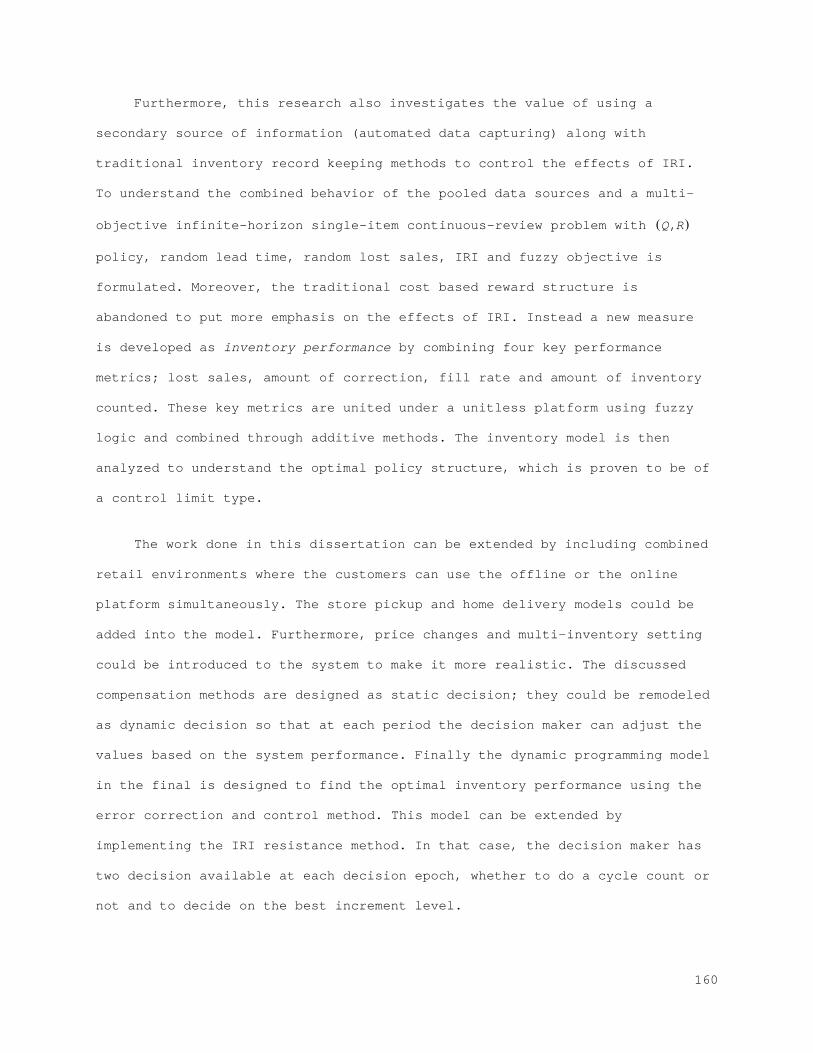
Furthermore, this research also investigates the value of using a
secondary source of information (automated data capturing) along with
traditional inventory record keeping methods to control the effects of IRI.
To understand the combined behavior of the pooled data sources and a multi-
objective infinite-horizon single-item continuous-review problem with ( ),Q R
policy, random lead time, random lost sales, IRI and fuzzy objective is
formulated. Moreover, the traditional cost based reward structure is
abandoned to put more emphasis on the effects of IRI. Instead a new measure
is developed as inventory performance by combining four key performance
metrics; lost sales, amount of correction, fill rate and amount of inventory
counted. These key metrics are united under a unitless platform using fuzzy
logic and combined through additive methods. The inventory model is then
analyzed to understand the optimal policy structure, which is proven to be of
a control limit type.
The work done in this dissertation can be extended by including combined
retail environments where the customers can use the offline or the online
platform simultaneously. The store pickup and home delivery models could be
added into the model. Furthermore, price changes and multi-inventory setting
could be introduced to the system to make it more realistic. The discussed
compensation methods are designed as static decision; they could be remodeled
as dynamic decision so that at each period the decision maker can adjust the
values based on the system performance. Finally the dynamic programming model
in the final is designed to find the optimal inventory performance using the
error correction and control method. This model can be extended by
implementing the IRI resistance method. In that case, the decision maker has
two decision available at each decision epoch, whether to do a cycle count or
not and to decide on the best increment level.
160