QuickTime™ and aTIFF (Uncompressed) decompressor

are needed to see this picture.

Results from the Carbon Cycle Data Assimilation System

(CCDAS)

3FastOpt42

Marko Scholze1, Peter Rayner2, Wolfgang Knorr1

Heinrich Widmann3, Thomas Kaminski4 & Ralf Giering4

1

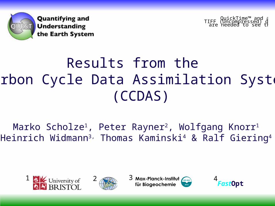
Methodology sketchCCDAS – Carbon Cycle Data Assimilation

System

CO2 stationconcentration

Biosphere Model:BETHY

Atmospheric Transport Model: TM2

Misfit to observations

Model parameter

Fluxes

Misfit 1 Forward Modeling:

Parameters –> Misfit

Inverse Modeling:

Parameter optimization

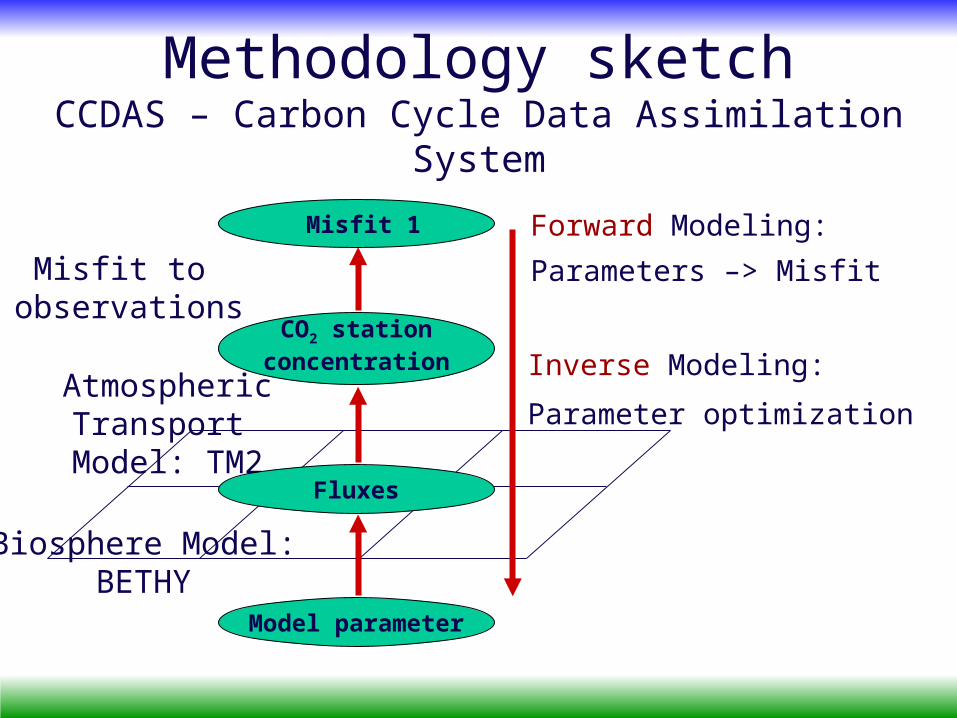
CCDAS set-up

Background fluxes:1. Fossil emissions (Marland et al., 2001 und Andres et al., 1996)2. Ocean CO2 (Takahashi et al., 1999 und Le Quéré et al., 2000)3. Land-use (Houghton et al., 1990)

Transport Model TM2 (Heimann, 1995)

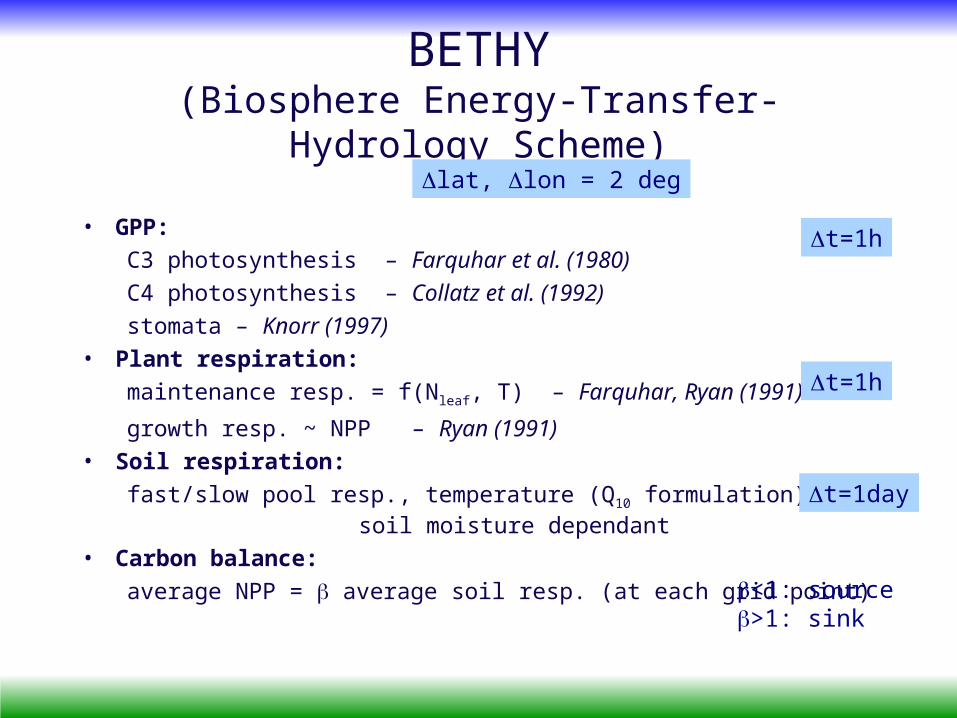
BETHY(Biosphere Energy-Transfer-

Hydrology Scheme)

• GPP:C3 photosynthesis – Farquhar et al. (1980)C4 photosynthesis – Collatz et al. (1992)stomata – Knorr (1997)

• Plant respiration:maintenance resp. = f(Nleaf, T) – Farquhar, Ryan (1991)

growth resp. ~ NPP – Ryan (1991) • Soil respiration:

fast/slow pool resp., temperature (Q10 formulation) and soil moisture dependant

• Carbon balance:average NPP = average soil resp. (at each grid point)<1: source

>1: sink

t=1h

t=1h

t=1day

lat, lon = 2 deg

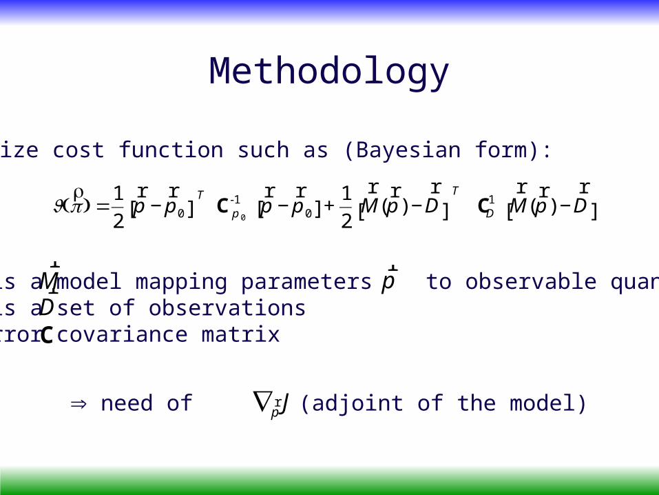
Methodology

Minimize cost function such as (Bayesian form):

€

J ( r p) =

1

2

r p −

r p 0[ ]

T Cp 0

-1 r p −

r p 0[ ] +

1

2

r M (

r p ) −

r D [ ]

T

CD-1

r M (

r p ) −

r D [ ]

where- is a model mapping parameters to observable quantities- is a set of observations- error covariance matrixC

DrMr

pr

need of (adjoint of the model)Jpr∇

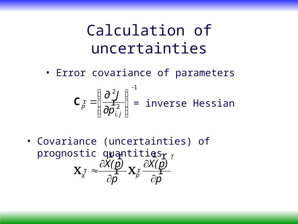
Calculation of uncertainties

• Error covariance of parameters1

2

2−

⎪⎭

⎪⎬⎫

⎪⎩

⎪⎨⎧

=ji,

p pJ

rr

∂∂

C = inverse Hessian

T

pX p)p(X

p)p(X

rrr

rrr

rr

∂∂

∂∂

≈ CC

• Covariance (uncertainties) of prognostic quantities

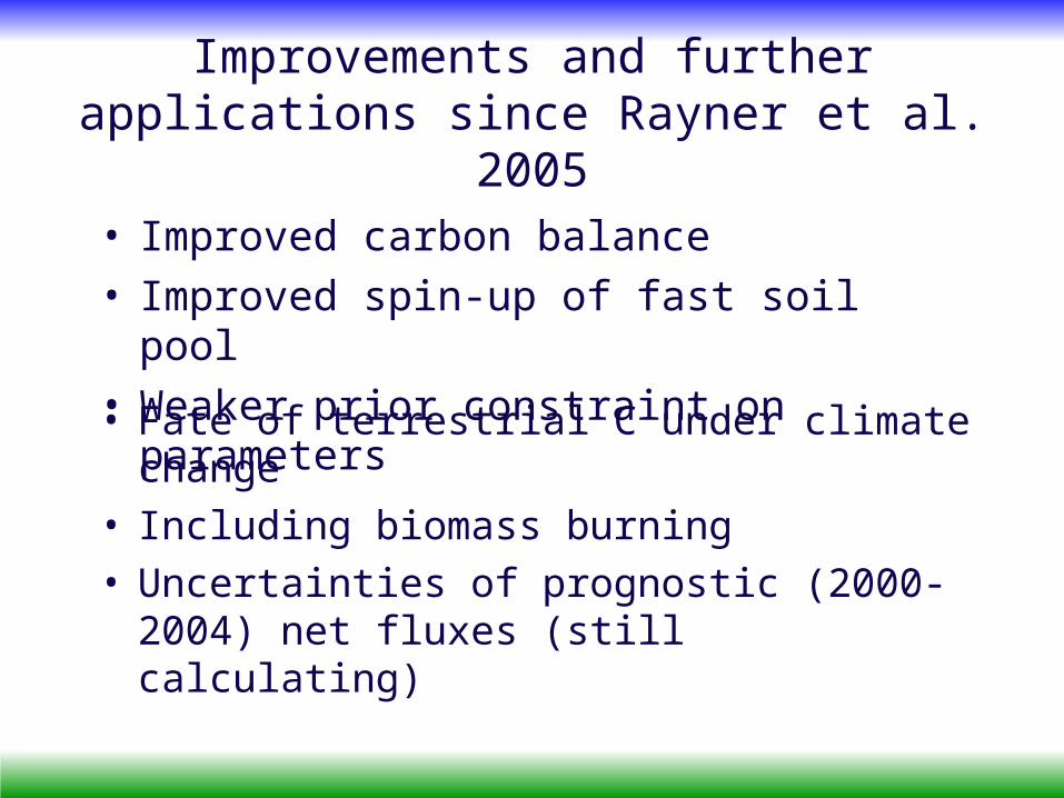
• Fate of terrestrial C under climate change• Including biomass burning• Uncertainties of prognostic (2000-2004) net

fluxes (still calculating)

Improvements and further applications since Rayner et al.

2005• Improved carbon balance• Improved spin-up of fast soil pool• Weaker prior constraint on parameters

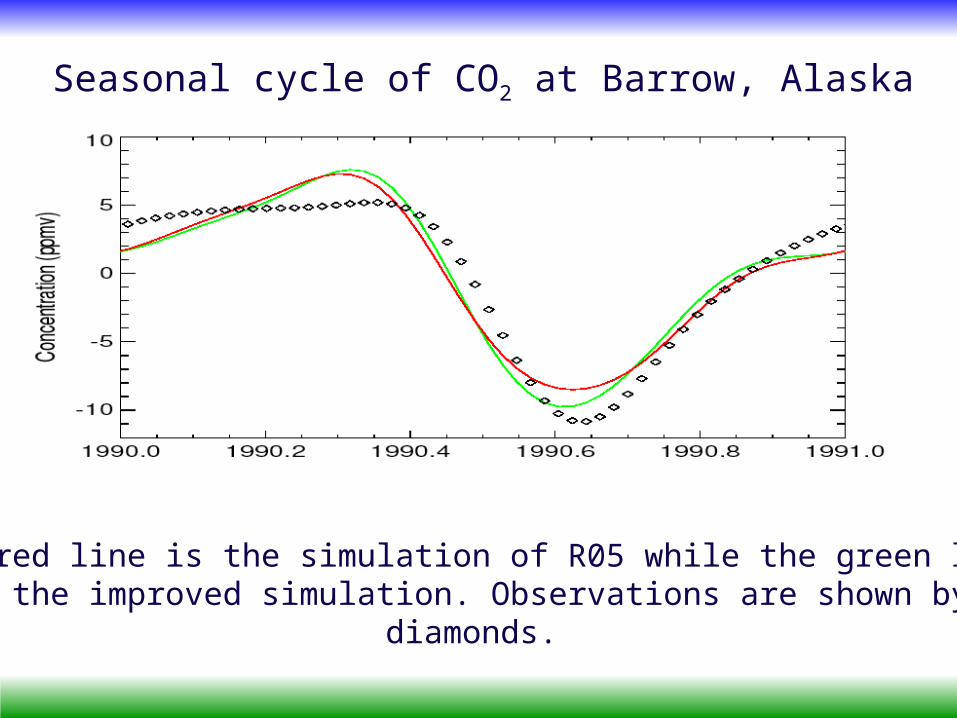
Seasonal cycle of CO2 at Barrow, Alaska

The red line is the simulation of R05 while the green lineIs the improved simulation. Observations are shown by

diamonds.

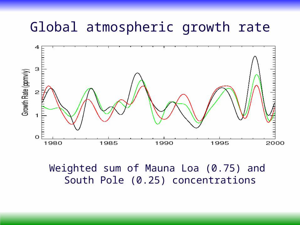
Global atmospheric growth rate

Weighted sum of Mauna Loa (0.75) and South Pole (0.25) concentrations

Parameters I

• 3 PFT specific parameters (Jmax, Jmax/Vmax and )

• 18 global parameters• 56 parameters in all plus 1 initial value

(offset)

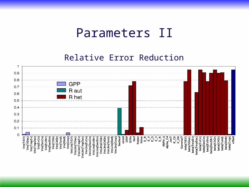
Parameters II

Relative Error Reduction

Some values of global fluxes

1980-2000 (prior)

1980-1999R05

New

GPPNPPFast Resp.Slow Resp.

135.768.1853.8314.46

134.840.5527.410.69

144.764.9225.736.9

NEP -0.11 2.45 2.32

Value Gt C/yr

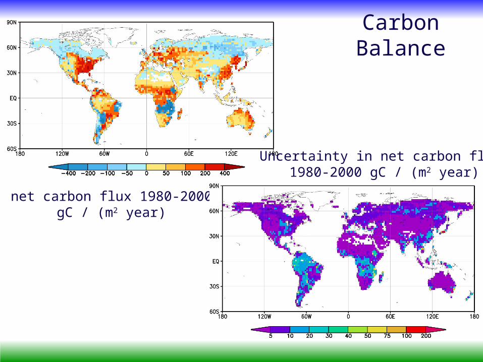
Carbon Balance

net carbon flux 1980-2000gC / (m2 year)

Uncertainty in net carbon flux 1980-2000 gC / (m2 year)

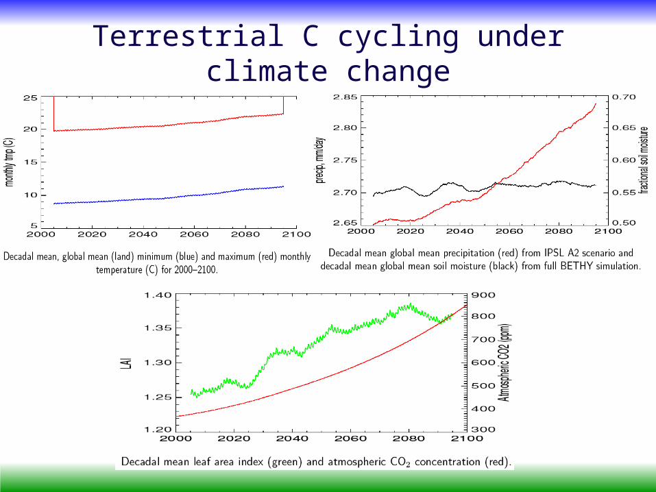
Terrestrial C cycling under climate change

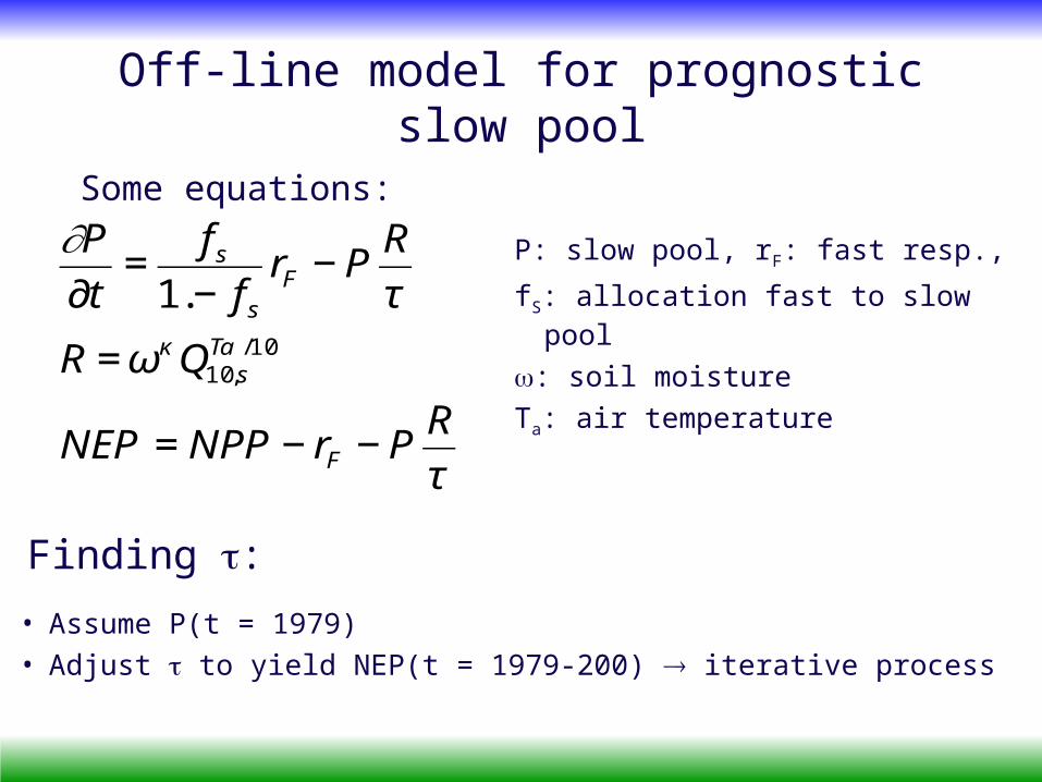
Off-line model for prognostic slow pool

€

∂P

∂t=

f s

1.− f s

rF − PR

τ

R = ωκ Q10,sTa /10

NEP = NPP − rF − PR

τ

Some equations:

P: slow pool, rF: fast resp.,

fS: allocation fast to slow pool

: soil moistureTa: air temperature

Finding :• Assume P(t = 1979)• Adjust to yield NEP(t = 1979-200) iterative process

Initial slow pool size

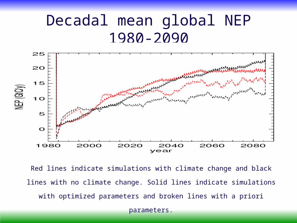
Decadal mean global NEP 1980-2090

Red lines indicate simulations with climate change and black

lines with no climate change. Solid lines indicate simulations

with optimized parameters and broken lines with a priori

parameters.

Including biomass burning

• A biomass burning climatology (monthly resolved) based on the v. d. Werf data is used as a yearly basis function for the optimisation

• Land is divided into the 11 TransCom-3 regions• That means: 11 regions * 21 yr = 231 additional

parameters

van der Werf et al., 2004, Continental-Scale Partitioning of fire emissions during the 1997 to 2001 El Niño/La Niña Period. Science, 303, 73-76.

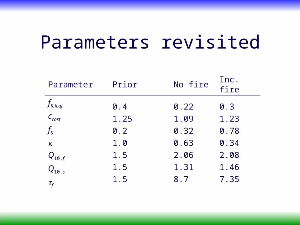
Parameters revisited

Parameter Prior No fireInc. fire

fR,leaf

ccost

fS

Q10,f

Q10,s

f

0.41.250.21.01.51.51.5

0.221.090.320.632.061.318.7

0.31.230.780.342.081.467.35

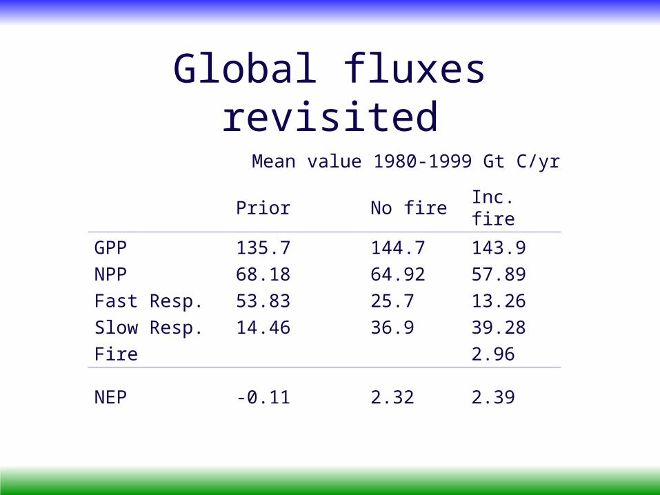
Global fluxes revisited

Prior No fireInc. fire

GPPNPPFast Resp.Slow Resp.Fire

135.768.1853.8314.46

144.764.9225.736.9

143.957.8913.2639.282.96

NEP -0.11 2.32 2.39

Mean value 1980-1999 Gt C/yr

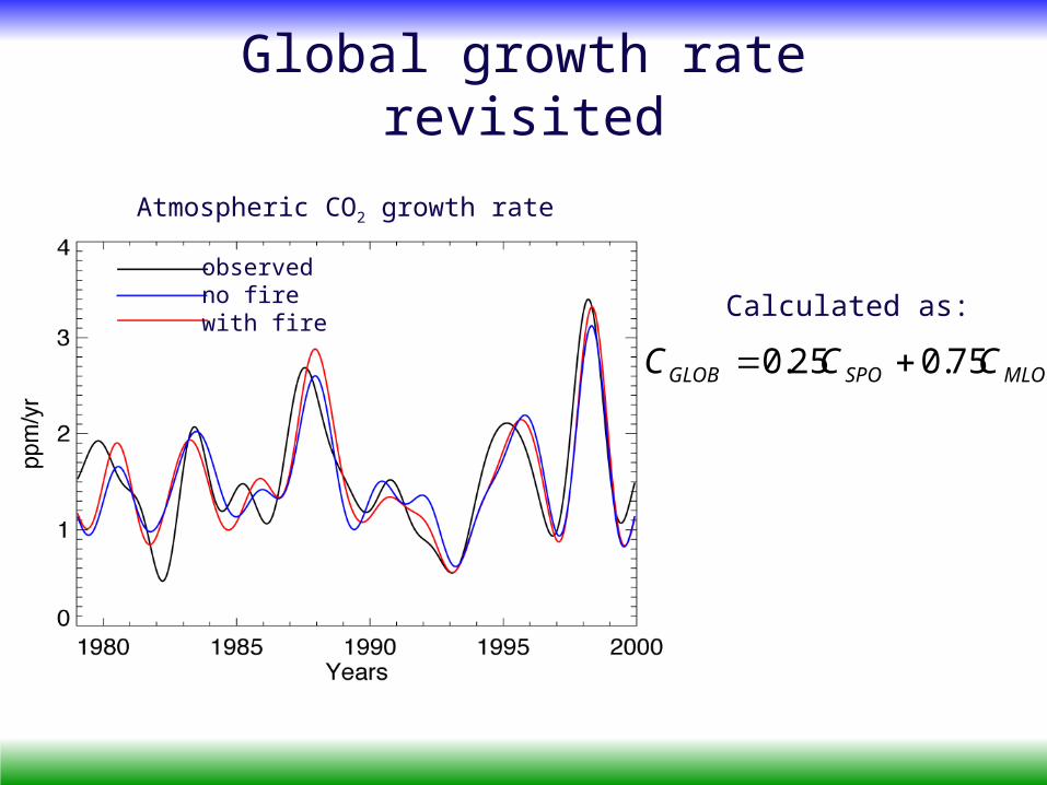
Global growth rate revisited

Calculated as:

Atmospheric CO2 growth rate

MLOSPOGLOB CCC 75.025.0 +=

observedno firewith fire

blue bars CCDAS red bars v. d. Werf et al.

Interannual variability in biomass burning estimate

year

0.00

0.50

1.00

1.50

2.00

2.50

3.00

3.50

4.00

4.50

19801981198219831984198519861987198819891990199119921993199419951996199719981999

Gt

C/y

r

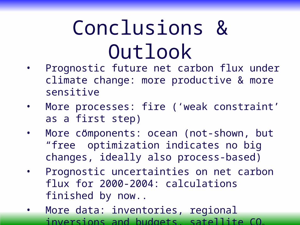
Conclusions & Outlook

• Prognostic future net carbon flux under climate change: more productive & more sensitive

• More processes: fire (‘weak constraint’ as a first step)

• More components: ocean (not-shown, but “free” optimization indicates no big changes, ideally also process-based)

• Prognostic uncertainties on net carbon flux for 2000-2004: calculations finished by now..

• More data: inventories, regional inversions and budgets, satellite CO2 columns, isotopes, O2/N2