FastOpt

A prototype Global Carbon Cycle Data Assimilation

System (CCDAS)

Marko Scholze1, Wolfgang Knorr2, Peter Rayner3,Thomas Kaminski4, Ralf Giering4

1 2 3 4

FastOpt

Overview

• Top-down vs. bottom-up

• Gradient method and optimisation

• Results: Optimal fluxes

• Uncertainties in parameters + results

• Uncertainties in fluxes + results

• Possible assimilation of flux data

• Conclusions and Outlook

FastOpt

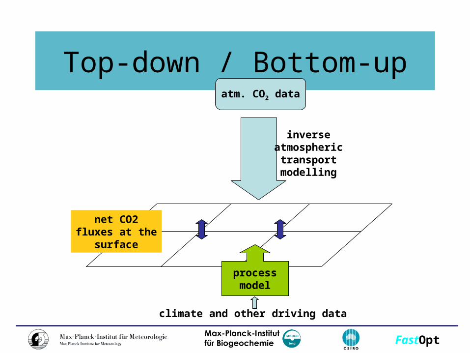
Top-down / Bottom-upatm. CO2 data

inverseatmospheric

transportmodelling

net CO2fluxes at the

surface

processmodel

climate and other driving data

FastOpt

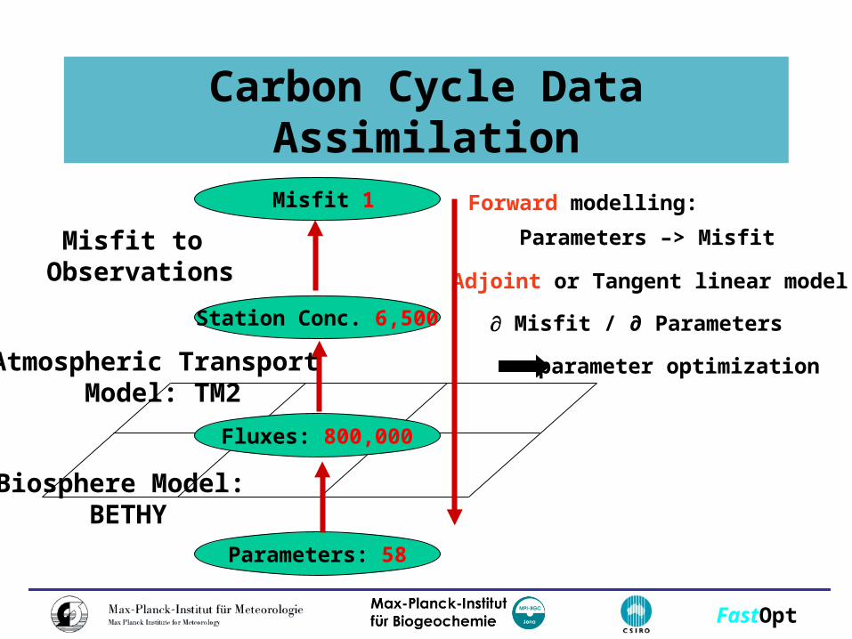
Carbon Cycle Data Assimilation

Biosphere Model: BETHY

Atmospheric Transport Model: TM2

Misfit to Observations

Parameters: 58

Fluxes: 800,000

Station Conc. 6,500

Misfit 1 Forward modelling:

Parameters –> Misfit

Adjoint or Tangent linear model:

Misfit / ∂ Parameters

parameter optimization

FastOpt

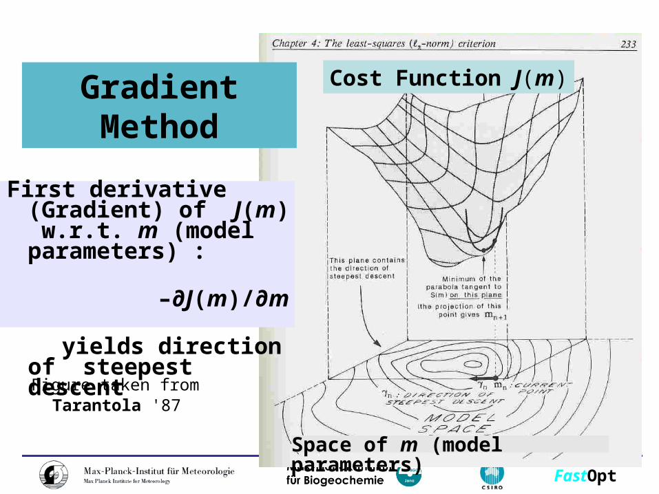
Figure taken from Tarantola '87

Space of m (model parameters)

First derivative (Gradient) of J(m) w.r.t. m (model parameters) :

–∂J(m)/∂m yields direction of steepest

descent

Gradient Method

Cost Function J(m)

FastOpt

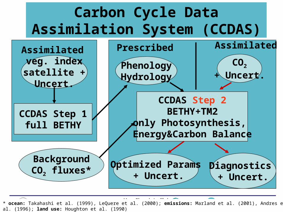
Carbon Cycle Data Assimilation System (CCDAS)

CCDAS Step 2BETHY+TM2

only Photosynthesis, Energy&Carbon Balance

CO2

+ Uncert.

Optimized Params + Uncert.

Diagnostics + Uncert.

veg. indexsatellite +Uncert.

CCDAS Step 1full BETHY

PhenologyHydrology

AssimilatedPrescribedAssimilated

BackgroundCO2 fluxes*

* * ocean: Takahashi et al. (1999), LeQuere et al. (2000); emissions: Marland et al. (2001), Andres et al. (1996); land use: Houghton et al. (1990)

FastOpt

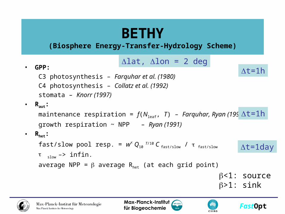
BETHY(Biosphere Energy-Transfer-Hydrology Scheme)

• GPP:

C3 photosynthesis – Farquhar et al. (1980)

C4 photosynthesis – Collatz et al. (1992)

stomata – Knorr (1997)

• Raut:

maintenance respiration = f(Nleaf, T) – Farquhar, Ryan (1991)

growth respiration ~ NPP – Ryan (1991)

• Rhet:

fast/slow pool resp. = wQ10 T/10 C fast/slow / fast/slow

slow –> infin.

average NPP = average Rhet (at each grid point)

<1: source>1: sink

t=1h

t=1h

t=1day

lat, lon = 2 deg

FastOpt

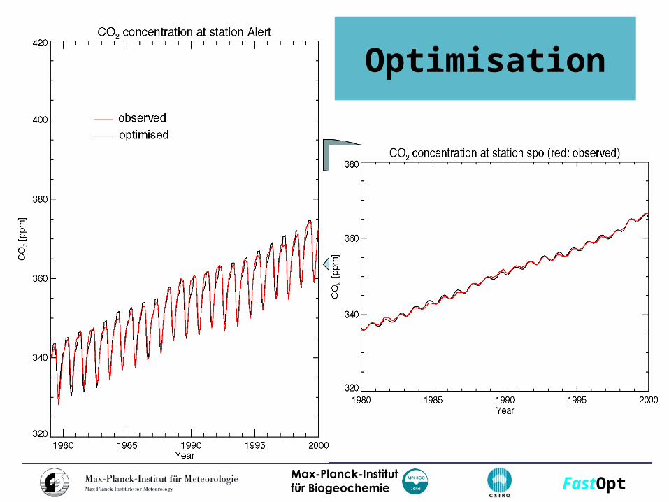
Optimisation

FastOpt

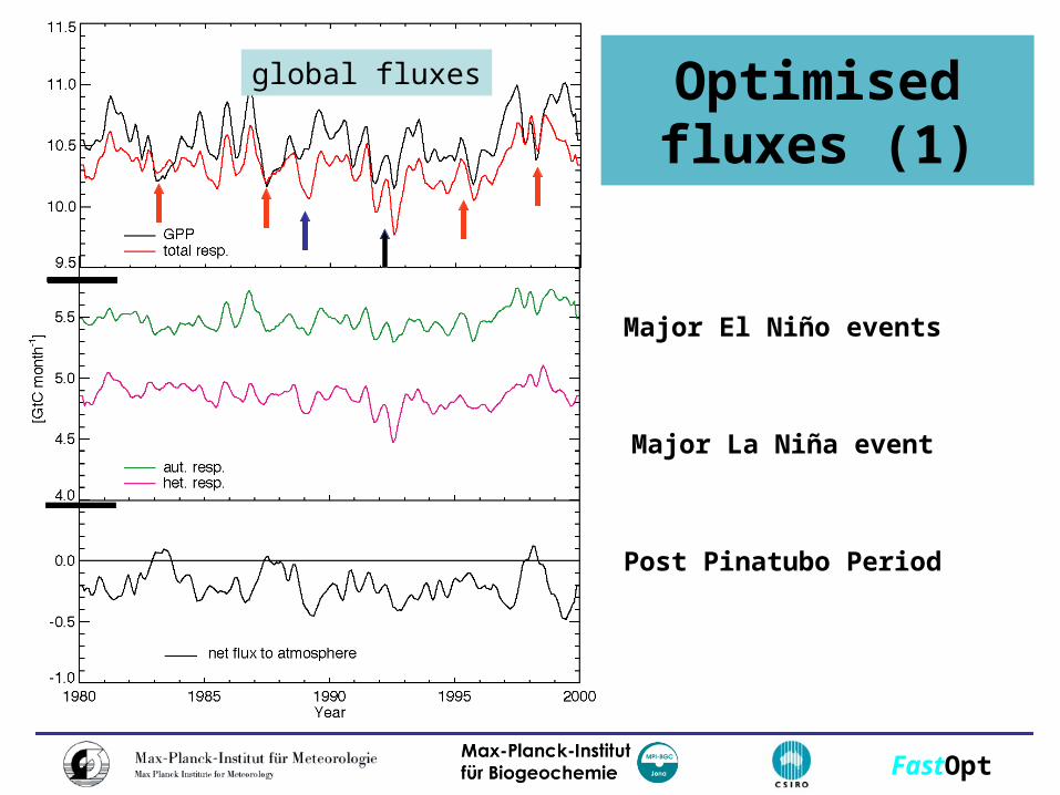
Optimised fluxes (1)

global fluxes

Major El Niño events

Major La Niña event

Post Pinatubo Period

FastOpt

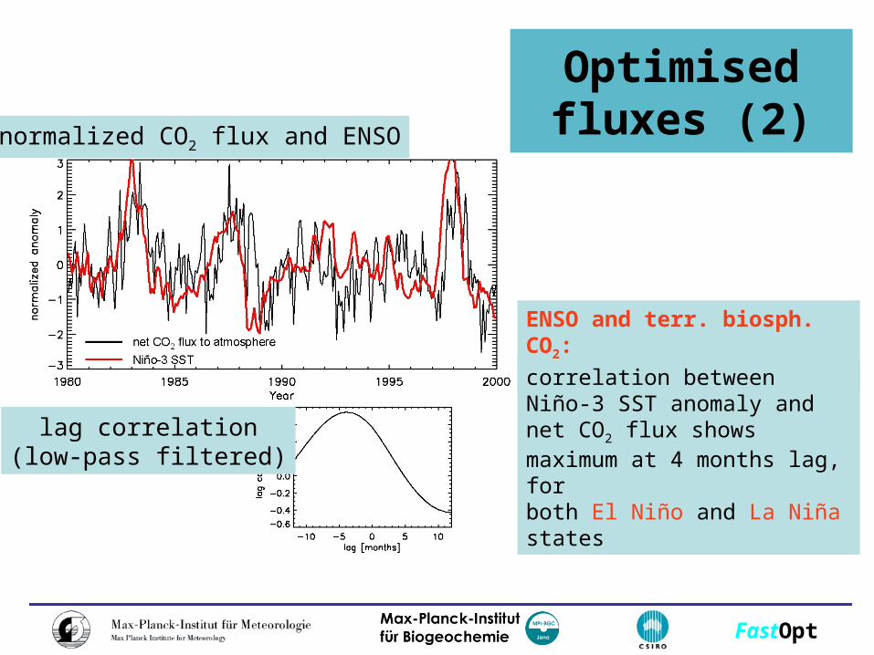
Optimised fluxes (2)normalized CO2 flux and ENSO

ENSO and terr. biosph. CO2:correlation seems strong

lag correlation(low-pass filtered)

correlation between Niño-3 SST anomaly and net CO2 flux shows maximum at 4 months lag, forboth El Niño and La Niña states

FastOpt

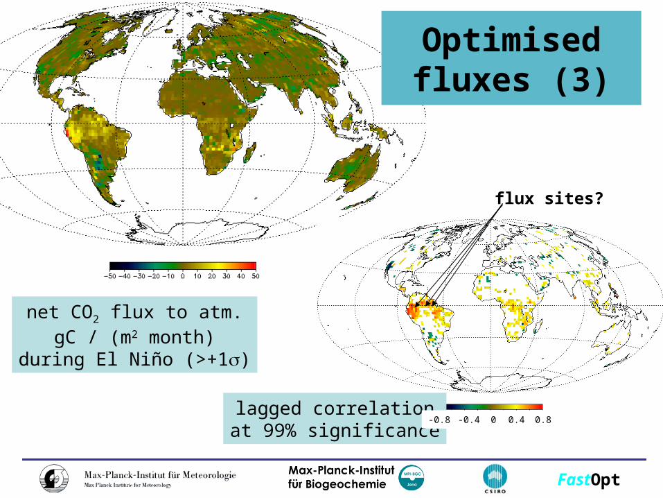
net CO2 flux to atm.gC / (m2 month)

during El Niño (>+1)

Optimised fluxes (3)

lagged correlationat 99% significance

-0.8 -0.4 0 0.4 0.8

flux sites?

FastOpt

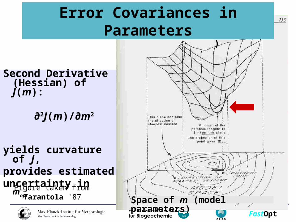
Figure taken from Tarantola '87

J(x)

Second Derivative (Hessian) of J(m):

∂2J(m)/∂m2 yields curvature of J,provides estimateduncertainty in m

opt

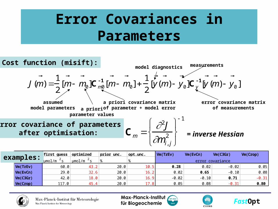
Error Covariances in Parameters

Space of m (model parameters)

FastOpt

Error Covariances in Parameters

first guess optimized prior unc. opt.unc. Vm(TrEv) Vm(EvCn) Vm(C3Gr) Vm(Crop)

µmol/m2s µmol/m2s % %Vm(TrEv) 60.0 43.2 20.0 10.5 0.28 0.02 -0.02 0.05Vm(EvCn) 29.0 32.6 20.0 16.2 0.02 0.65 -0.10 0.08Vm(C3Gr) 42.0 18.0 20.0 16.9 -0.02 -0.10 0.71 -0.31Vm(Crop) 117.0 45.4 20.0 17.8 0.05 0.08 -0.31 0.80

error covarianceexamples:

Cost function (misift):

J(

m ) 1

2[m

m 0]Cm0-1 [

m

m 0] 1

2[y (

m )

y 0]Cy-1 [

y (

m )

y 0 ]

model diagnostics

error covariance matrixof measurements

measurements

assumedmodel parameters

a priori covariance matrixof parameter + model errora priori

parameter values

Error covariance of parametersafter optimisation:

Cm 2J

mi, j2

1

= inverse Hessian

FastOpt

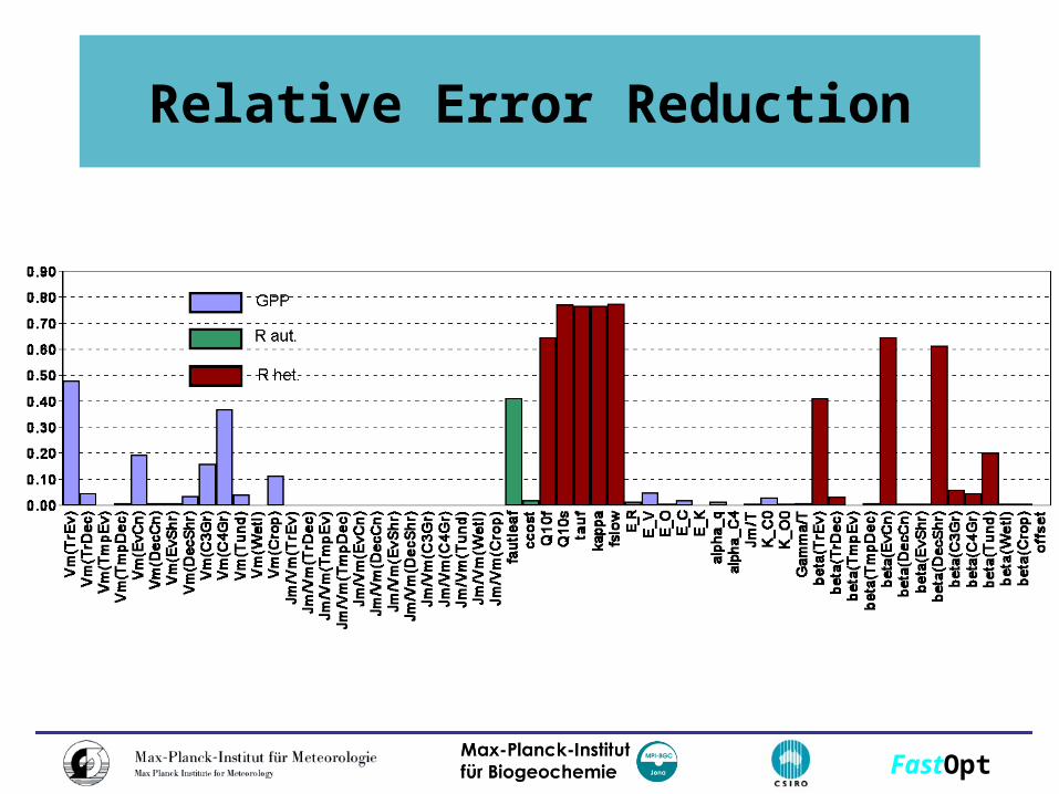
Relative Error Reduction

FastOpt

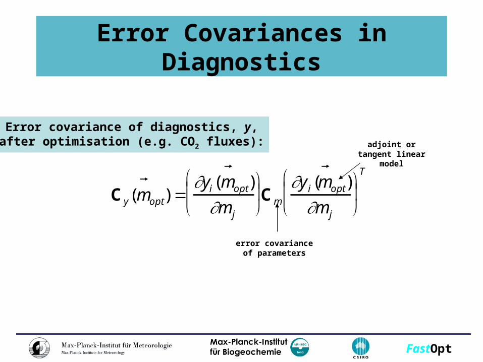
Error Covariances in Diagnostics

Error covariance of diagnostics, y,after optimisation (e.g. CO2 fluxes):

Cy(m opt)

yi(m opt)

m j

Cm

y i(m opt)

m j

T

error covarianceof parameters

adjoint ortangent linear

model

FastOpt

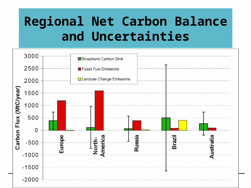
Regional Net Carbon Balance and Uncertainties

FastOpt

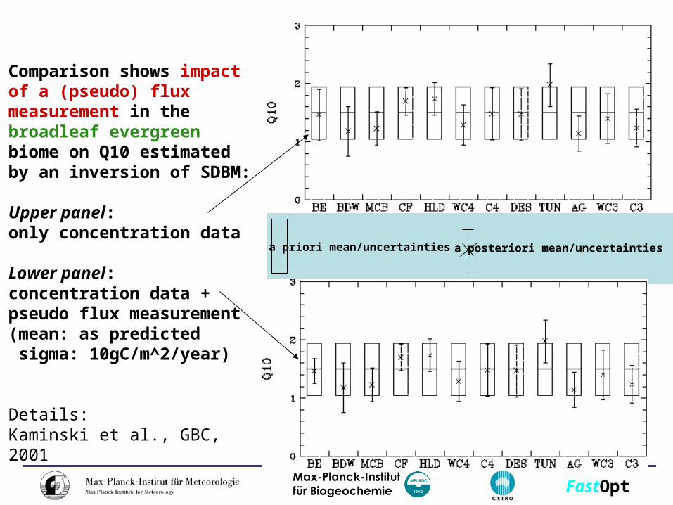
Comparison shows impact of a (pseudo) flux measurement in the broadleaf evergreen biome on Q10 estimated by an inversion of SDBM:

Upper panel: only concentration data

Lower panel: concentration data +pseudo flux measurement(mean: as predicted sigma: 10gC/m^2/year)

Details:Kaminski et al., GBC, 2001

a posteriori mean/uncertaintiesa priori mean/uncertainties

FastOpt

• CCDAS with 58 parameters can already fit 20 years

of CO2 concentration data

• Sizeable reduction of uncertainty for ~13 parameters

• terr. biosphere response to climate fluctuations

dominated by ENSO

• System can test model with uncertain parameters,

and deliver a posteriori uncertainties on parameters,

fluxes

Conclusions

FastOpt

• explore more parameter configurations• include fire as a process with uncertainties• need more constraints, e.g. eddy fluxes –>

reduce uncertainties• however: needs to solve scaling problem

(satellites?)• approach can be regionalized easily• extend approach to ocean carbon cycle• projection of uncertainties into future

Outlook