Embed Size (px)
Citation preview
Chapter 4
RESULTS AND DISCUSSION
The study entitled “Health and nutritional status of women and
preschool children in urban slums of Kochi” was conducted to appraise
the health‐nutritional profile of the sample and their interdependency and
also the extent of influence of living environment on the above
parameters. The data collected was analysed with this objective and the
results are discussed under the following heads:
4.1. Background information 4.1.1. Slum wise distribution of the sample 4.1.2. Family particulars 4.1.3. Educational and occupational status of parents 4.1.4. Economic profile 4.1.5. Housing condition 4.1.6. Hygienic practices 4.1.7. Availability and use of basic services 4.2. Nutritional and health status of women 4.2.1. Nutritional status of women 4.2.1.1 Nutritional anthropometry 4.2.1.2 Blood haemoglobin status 4.2.1.3 Dietary assessment 4.2.2. Health status of women 4.2.2.1 Incidence of health problems 4.2.2.2 Prevalence of goitre 4.2.2.3 Other reproductive health indicators 4.3. Nutritional and health status of preschool children 4.3.1. Nutritional status of preschoolers 4.3.1.1 Nutritional anthropometry 4.3.1.2 Blood haemoglobin status of preschool children 4.3.1.3 Dietary assessment of preschool children 4.3.2. Health status of preschool children 4.3.2.1 Nutritional disorders among preschool children 4.3.2.2 Childhood diseases 4.4 Correlation of health/nutritional status of mothers and
preschool children
Chapter 4 Results and Discussion
84
4.1. Background Information
The background information of sample including residing area,
family details, socioeconomic status, housing condition, availability and
use of basic services, were collected as these factors are known to have
either direct or indirect influence on health and well-being of people.
4.1.1 Slum wise distribution of the sample
The details on the sample distribution among the urban slums, the
study area, are presented in table 2.
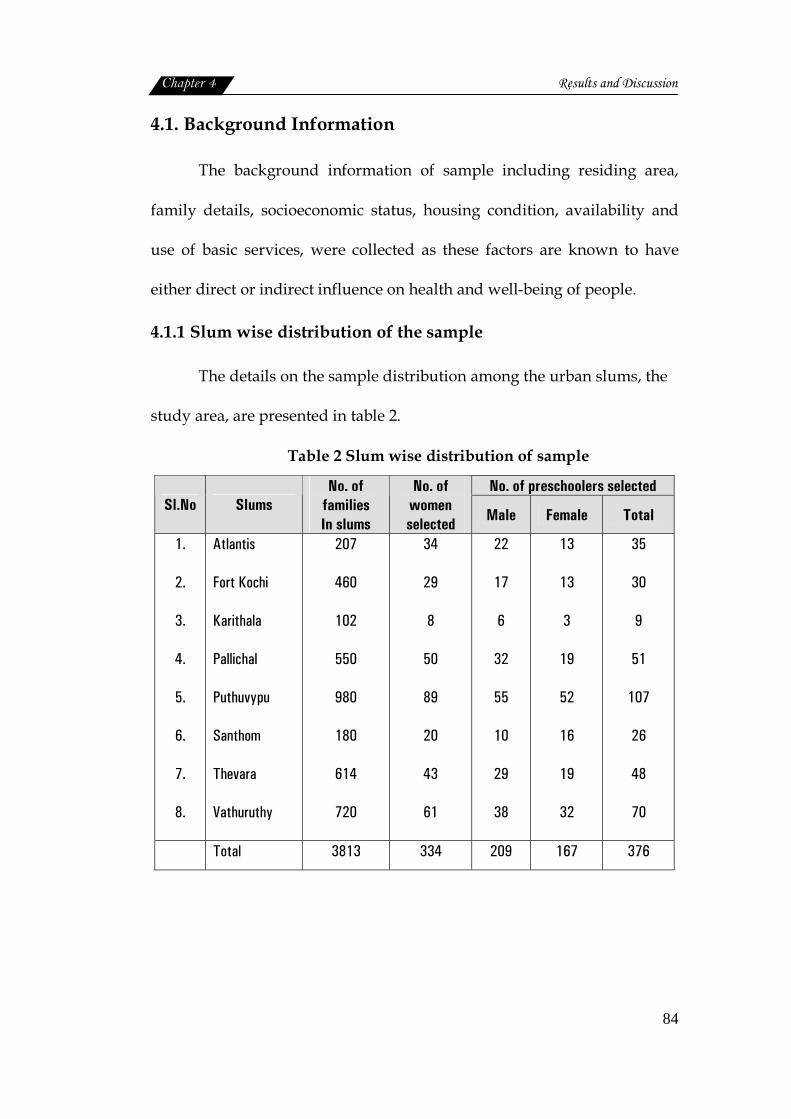
Table 2 Slum wise distribution of sample
No. of preschoolers selected Sl.No Slums
No. of families In slums
No. of women selected Male Female Total
1.
2.
3.
4.
5.
6.
7.
8.
Atlantis
Fort Kochi
Karithala
Pallichal
Puthuvypu
Santhom
Thevara
Vathuruthy
207
460
102
550
980
180
614
720
34
29
8
50
89
20
43
61
22
17
6
32
55
10
29
38
13
13
3
19
52
16
19
32
35
30
9
51
107
26
48
70
Total 3813 334 209 167 376
Chapter 4 Results and Discussion
85
The slums in different locations of Kochi city were included in the
study, since they are very crowded and thickly populated. The total
number of families in the selected slums (8 numbers) ranged between 102
to 980.
The sample population, women and their preschool children (3 to 5
years of age), was drawn from the eight slums, 334 women and 376
preschool children included in the sample of the total sample size of 710.
A good proportion of women (89 no’s) and preschoolers (107 no’s) were
from the Puthuvypu slum, which was the largest slum. This was followed
by Vathuruthy slum (61 women and 70 preschoolers) Karithala with the
lowest number of families, had least representation in the sample. The
total number of male children was 209 (55.6%) and female was 167
(44.4%).
4.1.2. Family Particulars:
The type of the family, size and religion are the aspects dealt with in
this section.
Type and size of the family
The details on family structure is given in table 3.

Chapter 4 Results and Discussion
86
Table 3 Distribution of sample based on type and size of the family
Sl.No. Particulars Frequency (n=334)
1.
Type of family
Nuclear
Joint
Extended
207 (62.0)
47 (14.0)
80 (24.0)
2.
Family Size
3 members
4-6 members
>6 members
64 (19.1)
268 (80.3)
2 (0.6)
3.
Number of children
One child
Two
Three
Four
Five
Ten
64 (19.1)
222 (66.5)
41 (12.3)
5 (1.5)
1 (0.3)
1 (0.3)
(Numbers in parentheses indicate percentages)
As the table depicts 62.0 per cent of sample belonged to nuclear
family system followed by extended families (24.0%). Joint family system
was seen only among 14.0 percent of the sample. Hence nuclear family
system was more popular among the sample studied. Kotwal et al. (2008)
also stated that usually families in slums are nuclear type. Similar findings
were reported by NNMB (2002) and NNMB (2006).
Three among five households in India are nuclear. Nuclear
households are defined in NFHS-3 (2008) as households that are
comprised of a married couple or a man or a woman living alone or with
Chapter 4 Results and Discussion
87
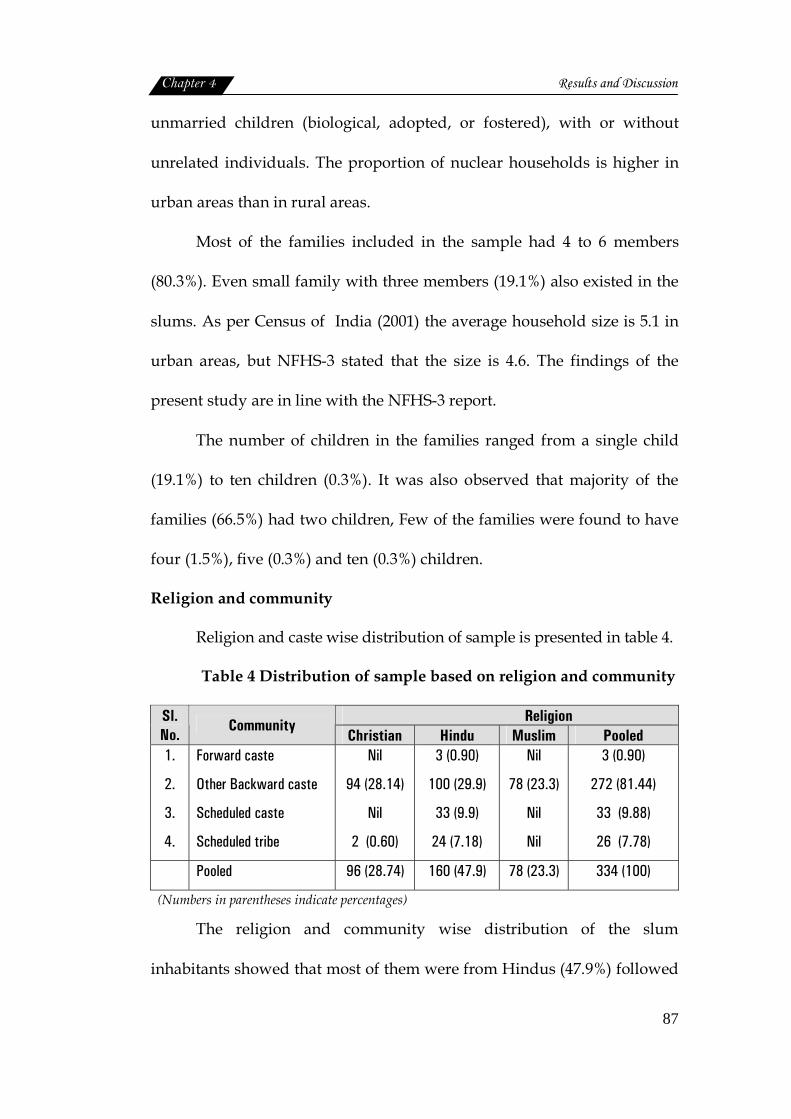
unmarried children (biological, adopted, or fostered), with or without
unrelated individuals. The proportion of nuclear households is higher in
urban areas than in rural areas.
Most of the families included in the sample had 4 to 6 members
(80.3%). Even small family with three members (19.1%) also existed in the
slums. As per Census of India (2001) the average household size is 5.1 in
urban areas, but NFHS-3 stated that the size is 4.6. The findings of the
present study are in line with the NFHS-3 report.
The number of children in the families ranged from a single child
(19.1%) to ten children (0.3%). It was also observed that majority of the
families (66.5%) had two children, Few of the families were found to have
four (1.5%), five (0.3%) and ten (0.3%) children.
Religion and community
Religion and caste wise distribution of sample is presented in table 4.
Table 4 Distribution of sample based on religion and community
Religion Sl. No.
Community Christian Hindu Muslim Pooled
1.
2.
3.
4.
Forward caste
Other Backward caste
Scheduled caste
Scheduled tribe
Nil
94 (28.14)
Nil
2 (0.60)
3 (0.90)
100 (29.9)
33 (9.9)
24 (7.18)
Nil
78 (23.3)
Nil
Nil
3 (0.90)
272 (81.44)
33 (9.88)
26 (7.78)
Pooled 96 (28.74) 160 (47.9) 78 (23.3) 334 (100)
(Numbers in parentheses indicate percentages)
The religion and community wise distribution of the slum
inhabitants showed that most of them were from Hindus (47.9%) followed
Chapter 4 Results and Discussion
88
by Christians (28.74%) and Muslims (23.3%). Whereas caste distribution
indicated that people belonged to other backward caste (81.44%)
outnumbered other communities like schedule caste (9.88%), schedule
tribe (7.78%) and forward caste (0.90%).
4.1.3. Educational and occupational status of parents
Education and Occupation
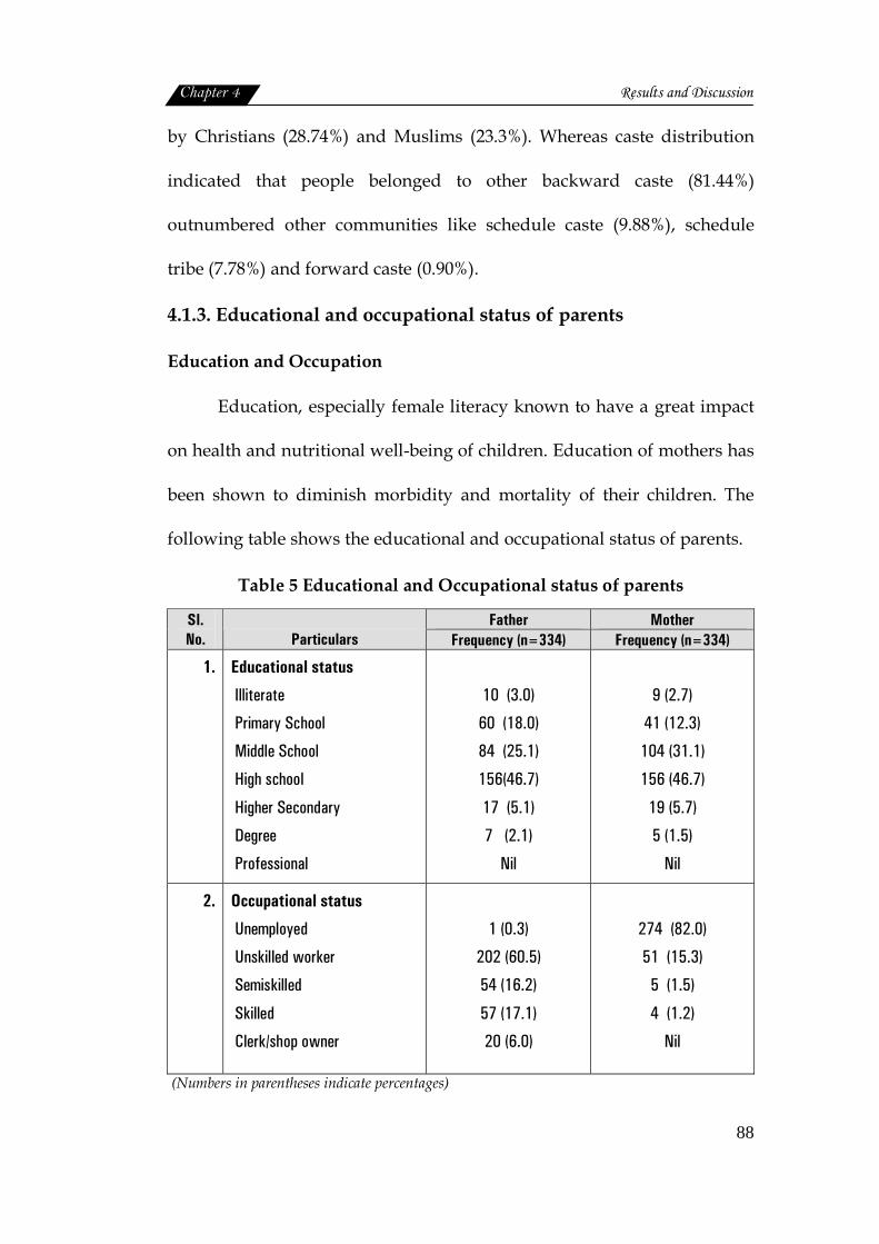
Education, especially female literacy known to have a great impact
on health and nutritional well-being of children. Education of mothers has
been shown to diminish morbidity and mortality of their children. The
following table shows the educational and occupational status of parents.
Table 5 Educational and Occupational status of parents
Father Mother Sl. No.
Particulars Frequency (n=334) Frequency (n=334)
1.
Educational status
Illiterate
Primary School
Middle School
High school
Higher Secondary
Degree
Professional
10 (3.0)
60 (18.0)
84 (25.1)
156(46.7)
17 (5.1)
7 (2.1)
Nil
9 (2.7)
41 (12.3)
104 (31.1)
156 (46.7)
19 (5.7)
5 (1.5)
Nil
2.
Occupational status
Unemployed
Unskilled worker
Semiskilled
Skilled
Clerk/shop owner
1 (0.3)
202 (60.5)
54 (16.2)
57 (17.1)
20 (6.0)
274 (82.0)
51 (15.3)
5 (1.5)
4 (1.2)
Nil
(Numbers in parentheses indicate percentages)
Chapter 4 Results and Discussion
89
Educational status of slum dwellers showed that nearly half of the
men (46.7%) as well as women (46.7%) had education upto high school
level, followed by middle school education and primary school education.
Only 2.1 percent of men and 1.5 percent of women were educated upto
degree level. There were no professionally qualified people. But 3.0
percent of men and 2.7 percent of women were found to be illiterate.
In Kerala, however the total literacy rate among the study
population was 94.2 percent for men and 87.86 for women. High female
literacy rate in Kerala has already been reported by Census of India (2001).
Literacy has been considered as one of the most important attributes
for social development. Educational deprivation of slum population and
gender discrimination in education with females having less access to
education than men were highlighted/emphasized by Kumar et al. (2007).
According to the authors this is common phenomenon observed not only
in slums but also outside the slums in the city.
There is a strong relationship between women’s work lives and
health. Lack of education compel women to join low paid sectors
(Kotwal et al., 2008). The families’ occupational status showed that most of
the men were unskilled workers (60.5%), some of them were fish sellers or
fishermen, while skilled (17.1%) as well as semiskilled workers (16.2%)
were also present in the slums.
Chapter 4 Results and Discussion
90
Data on occupational status of women showed that most of them
were unemployed (82.0%), whereas unskilled workers (15.3%) were found
to be more than semiskilled (1.5%) and skilled workers (1.2%). Among the
unskilled, most of them were working as house maids, coolies etc. Low
income was a compelling factor for the women folk to opt for petty jobs in
unorganized sector (Kotwal et al., 2008).
Mohanthy and Mohanthy (2005) also found that majority of the
slum dwellers were migrants from different places within the country and
were unskilled workers with low occupational status and low income. In
Kochi urbanisation has been associated with a process of casualisation of
labour. Kotwal et al. (2008) also reported that slum dwellers were mostly
labourers who failed to find regular employment in the modern organized
sector. Besides, joblessness is found to be basically a problem of educated
youth, leading to their migration to other parts of India (Prakash, 2002).
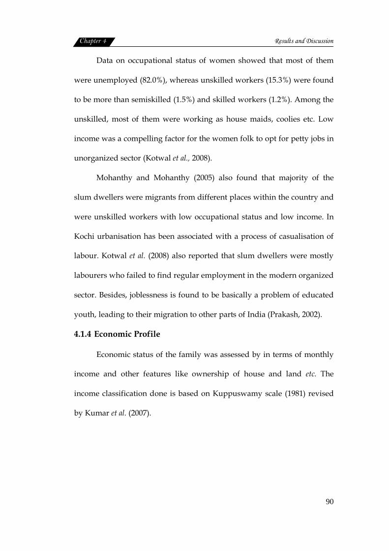
4.1.4 Economic Profile
Economic status of the family was assessed by in terms of monthly
income and other features like ownership of house and land etc. The
income classification done is based on Kuppuswamy scale (1981) revised
by Kumar et al. (2007).
Chapter 4 Results and Discussion
91
Table 6 Economic status of the sample
Sl.No Particulars Frequency (n=334) 1.
2.
3.
4.
Monthly Income (Rupees)
Below 980
981-2935
2936-4893
4894-7322
Land Ownership
Owned
Not owned
Tenure status
Owned
Rented
Lease
Saving /Debts
Savings
Debts
7(2.1)
260(77.8)
67(20.1)
Nil
271(81.1)
63(18.9)
271(81.1)
50(15.0)
13(3.9)
127(38.0)
235(70.4)
(Numbers in parentheses indicate percentages)
Economic status of the family showed that majority (77.8%) of the
family had a monthly income between ` 981/- to ` 2935/-, one out of five
of the sample had income in the range of ` 2936/- and ` 4893/-. Families
with income less than ` 980 (2.1%) was found to be less.
As UN Habitat (2002) reported that slums are manifestations of
urban poverty. The slum dwellers are considered as the poorest section of
the urban society (Kumar, 2006). But Mitra et al. (2006) stated that slums
do not accommodate all of the urban poor nor are all slum dwellers
always poor.

Chapter 4 Results and Discussion
92
The slum population usually faces land and housing shortage. In
the present study it was observed that majority of the families (81.1%)
owned land with limited area which has been issued to them. This comes
to approximately three and half cents. The house was also built in this
land. The rest of the samples migrated from nearby state and they lacked
land ownership (18.9%).
Tenure status of the sample showed that house ownership was
found among 81.1 percent. Other than these, houses were on rental
(15.0%) or lease (3.9%) basis. According to NSSO (2002) 60 percent of the
urban households owned the dwelling units. A study conducted by
Chandramouli (2003) in Chennai revealed that 40 percent of houses in
slums are rented and 3 percent are neither rented nor owned.
Usually slum dwellers earn their wages on daily basis, and it is very
inadequate to make. Inspite of this situation few families (38.0%) had the
habit of saving money for future. But majority (62.0%) of them had no
savings. UN Habitat Report (2003) and South Asia Analysis Group (2006)
also reported that slums are largely a physical manifestation of urban
poverty and very poor people live in slums.
Other family assets
Other possessions of the family ranging from simple labour saving
home appliances to vehicles for transportation was noted as asset of the
family. The details are given in the table below.
Chapter 4 Results and Discussion
93
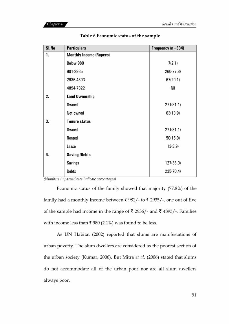
Table 7 Distribution of the sample based on family assets
Sl.No. Particulars Frequency (n=334)
1.
2.
3.
4.
5.
6.
7.
8.
Cycle/ Two wheeler
Radio
Television
Telephone
Refrigerator
Washing machine
Sewing machine
Mixer/Grinder
205 (61.4)
92 (27.5)
205 (61.4)
41(12.3)
34 (10.2)
5 (1.5)
31 (9.3)
112 (33.5)
(Numbers in parentheses indicate percentages)
Each family found to possess more than one asset listed in the table
7. Television was possessed by majority of the families (61.4%) while radio
was present only in 27.5 percent of families. Mixer /Grinder was used by
33.5 percent of families. Refrigerator was present only in 10.2 percent of
households. Only 12.3 percent had telephone, 9.3 percent sewing machine
and 1.5 percent had washing machine.
Socioeconomic position (Kuppuswamy Scale)
A strong association has been found between socioeconomic
position (SEP) and poor health status (WHO, 1995). Therefore
socioeconomic status of the families was computed using Kuppuswamy
scale (1981) revised by Kumar et al. (2007) which is given in appendix-VIII.
The sample were categorized accordingly and given in table 8.
Chapter 4 Results and Discussion
94
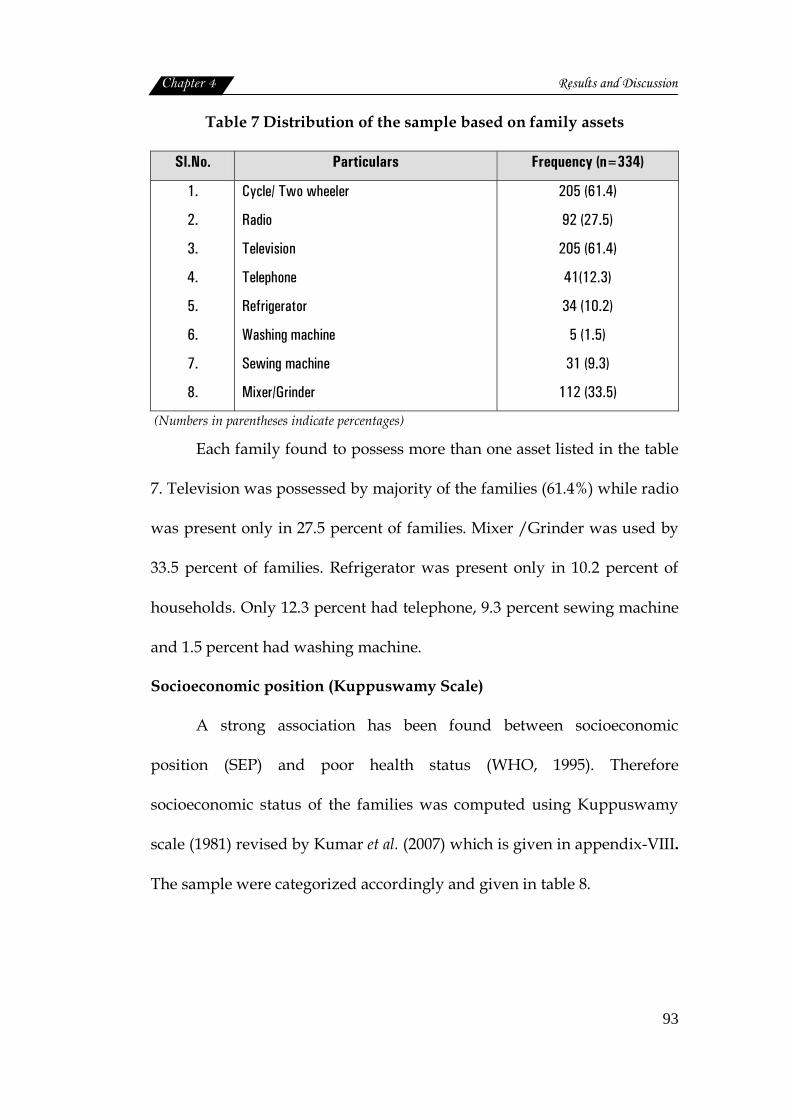
Table 8 Distribution of sample based on area and socioeconomic status
Socioeconomic status® Sl.No. Slums
Middle class Lower class 1.
2.
3.
4.
5.
6.
7.
8.
Atlantis
Fort Kochi
Karithala
Pallichal
Puthuvypu
Santhom
Thevara
Vathuruthy
12 (35.3)
5 (17.2)
Nil
7 (14.0)
3 (3.4)
2 (10.0)
11 (25.6)
2(3.3)
22 (64.7)
24 (82.8)
8 (100.0)
43 (86.0)
86 (96.6)
18 (90.0)
32 (74.4)
59 (96.7)
Pooled 42(12.57) 292 (87.42)
®Ref: Kuppuswamy scale(1981) revised by Kumar et al.(2007) (Numbers in parentheses indicate percentages)
As the table depicts, majority of slum dwellers (87.42%) had low
socioeconomic status as per Kuppuswamy scale (1981). Middle income
status was reported by 12.57 percent of families. None had high income
status. So the findings of Mitra et al. (2006) saying that slum do not
accommodate all urban poor; did not match with the present findings.
Socioeconomic status distribution among the individual slums showed
that 64.7 to 100 percent of families in the 8 selected slums had low
socioeconomic status with highest at Karithala (100.0%), Vathuruthy
(96.7%), Puthuvypu (96.6%) and Santhom (90.0%) colonies. In the rest of
the slums also majority, had only low socioeconomic status; middle class
status was reported by comparatively less number of families (35.3% to
3.3%) and none of the families in the slum found to have a high
socioeconomic status as per the Kuppuswamy scale (1981). Middle class
Chapter 4 Results and Discussion
95
families were comparatively low and it was distributed among Fort Kochi
(17.2%), Pallichal (14.0%), Puthuvypu (3.4%), Santhom (10.0%) and
Vathuruthy (3.3%).
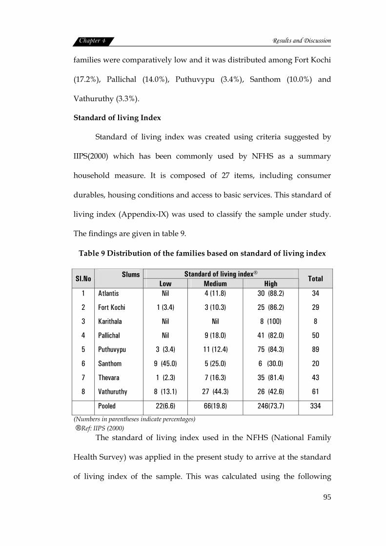
Standard of living Index
Standard of living index was created using criteria suggested by
IIPS(2000) which has been commonly used by NFHS as a summary
household measure. It is composed of 27 items, including consumer
durables, housing conditions and access to basic services. This standard of
living index (Appendix-IX) was used to classify the sample under study.
The findings are given in table 9.
Table 9 Distribution of the families based on standard of living index
Standard of living index® Sl.No Slums
Low Medium High Total
1
2
3
4
5
6
7
8
Atlantis
Fort Kochi
Karithala
Pallichal
Puthuvypu
Santhom
Thevara
Vathuruthy
Nil
1 (3.4)
Nil
Nil
3 (3.4)
9 (45.0)
1 (2.3)
8 (13.1)
4 (11.8)
3 (10.3)
Nil
9 (18.0)
11 (12.4)
5 (25.0)
7 (16.3)
27 (44.3)
30 (88.2)
25 (86.2)
8 (100)
41 (82.0)
75 (84.3)
6 (30.0)
35 (81.4)
26 (42.6)
34
29
8
50
89
20
43
61
Pooled 22(6.6) 66(19.8) 246(73.7) 334
(Numbers in parentheses indicate percentages) ®Ref: IIPS (2000)
The standard of living index used in the NFHS (National Family
Health Survey) was applied in the present study to arrive at the standard
of living index of the sample. This was calculated using the following
Chapter 4 Results and Discussion
96
variables like type of house, toilet facility, source of lighting, fuel used for
cooking, source of drinking water, separate room for cooking, ownership
of house ownership of land, livestock and ownership of durable goods
scoring method was used. A total scores ranging from zero to 14 refers to
low standard of living. The scores between 15 and 24 indicates medium
standard of living. High standard of living is arrived by a total score
ranging between 25 and 66.
The standard of living index thus computed clearly showed that
73.7 percent of the slum dwellers included in the study enjoyed a high
standard of living index. This is contrary to the socioeconomic status
calculated by Kuppuswamy Scale, where majority were grouped under
low status.
This distribution of families with high standard of living index
among the eight slums, showed a uniform trend i.e., a progressive
reduction in the number of families with declining of living standard
index. Only exception to this was Santhom colony, where more number of
families (45.0%) were categorized under low standard of living index.
Economic standard of living concerns the physical circumstances in
which people live, the goods and services they are able to consume, and
the economic resources they have access to. Basic necessities such as
adequate food, clothing and housing are fundamental to well being (South
Asia Analysis group, 2006).

Chapter 4 Results and Discussion
97
In the present study nearness to the urban sector and availability of
essential services accessibility and use of health care services due to high
female literacy rate may be the reason for the high standard of living index
and low socioeconomic status syndrome observed among the slum
population in Kochi city.
Majority of women who live in slums belong to lower socioeconomic
classes and either they have migrated to the city with the hope of better
means of livelihood or forced to migrate with their partners. Majority of them
having no education, skill and work experience, have no chance in the
competitive job. They pickup low paid jobs such as construction labourers,
domestic servants and casual factory workers. Inadequate income, poor
housing conditions, overcrowded environment, poor sanitation, occupational
hazards and stressful conditions are unfavorable to the health of women
residing slums (Kumar and Sinha, 2007).
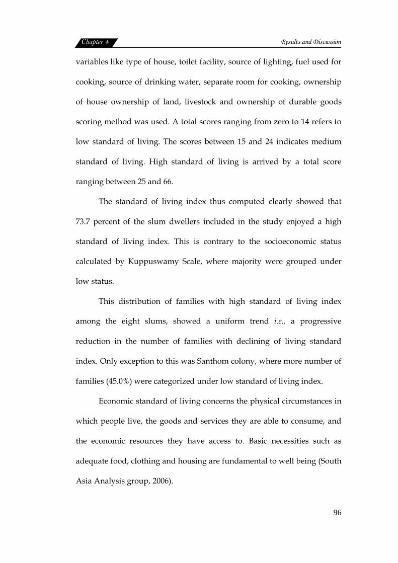
4.1.5 Housing condition
Housing plays an important role in the health of the individual.
Hence an attempt was made to procure information on the housing
conditions of the sample and presented in this section.
Type of house and facilities
The details are given in table 10.
Chapter 4 Results and Discussion
98
Table 10 Details on basic features of housing
Sl.No. Particulars Frequency(n=334) 1.
2.
3.
4.
5.
6.
7.
8.
9.
Type of house Kutcha Semi Pucca Pucca No. of rooms One room or multi purpose Two rooms Three rooms Separate kitchen Present Absent Storage area Present Absent Toilet Absent Separate Common for two houses Common for more than two houses Sanitation facility Pit toilet Flush toilet Open defecation Total area ≤100 sq.ft 100-300 sq.ft 300-500 sq.ft 500-700 sq.ft Plinth level Ground level 0-1Ft 1-2 Ft 2-3 Ft Height of ceiling Less than 6 feet 6-7 feet 7 feet and more
90 (27.0)
204 (61.0) 40 (12.0)
93 (27.8)
142 (42.5) 99 (29.6)
260 (77.8) 74 (22.2)
12 (3.59)
322 (96.41)
25 (7.5) 61 (18.3)
201 (60.2) 47 (14.1)
272 (81.4) 11 (3.3)
51 (15.3)
50 (15.0) 215 (64.3) 63 (18.9) 6 (1.8)
94 (28.1) 132 (39.5) 86 (25.7) 22 (6.6)
71 (21.3) 243 (72.8)
20 (6.0) (Numbers in parentheses indicate percentages)

Chapter 4 Results and Discussion
99
Type of House
Usually the houses in slums all over the world are of inferior
quality. In the present study the houses were mostly of semi pucca (61.0%)
or kutcha types (27.0%) A structure having walls and roof made of non
pucca materials was regarded as a kutcha structure (NSSO, 2004). Pucca
houses were only a few (12.0%), pucca structure was the one, having walls
and roofs made of pucca materials (NSSO, 2004).
The houses which had brick wall and reinforced cement concrete
roofs/tile roof were termed as pucca, while semi pucca houses where
those with brick wall with tin/asbestos roof, excluding thatch and
reinforced cement concrete roof. Kutcha houses where those with either
thatch roof or mud wall. NSSO (2004) reported that in urban slum areas,
65 percent of the dwellings are pucca and in Kerala it was 71 percent. In
the present study also pucca and semi pucca houses together constituted
73 percent. In urban India, NSSO (2002) also reported a fall in kutcha
construction from 18 percent during 1989-93 to 12 percent during 1998-
2002 and a rise in pucca constructions from 64 percent to 74 percent
(NSSO, 2002).
Rooms
The numbers of rooms were less in the case of slums. The study
revealed that about 42.5 percent of houses had two rooms, followed by
three room houses (29.6%). One room apartment was also found among
27.8 percent of houses. As per Census of India (2001) in urban areas of
Chapter 4 Results and Discussion
100
Kerala two room houses were seen among 23.4 percent, while one room
was observed among 9.1 percent. The availability of living space within
the house is also a vital parameter for good health (Chandramouli, 2003).
Kamla et al. (2009) reported that overcrowding in rooms leads to various
infections.
Kitchen
Separate kitchen is a necessity for each household, this was present
in the case of 77.8 percent of the houses in the slums while it was absent in
22.2 percent. Another essential feature of a kitchen is a raised cooking
platform, which was present in majority (63.8%) of houses and absent in
36.2 percent. This is comparable with the reports by Census of India (2001)
which states that majority of the households (95.4%) of Kerala. This trend
is extended to slums in Kerala also had separate kitchen. Kamla et al.
(2009) reported that separate kitchen was present in almost 70 percent of
the household than when compared with houses in slums (30%). The need
for separate kitchen was further stressed by Chandramouli (2003),
availability of a separate kitchen within the house and the type of fuel
used for cooking have a direct bearing on the incidence of respiratory
diseases especially among women who are directly exposed to smoke
emitted by fuels.
Storage area was found to be limited within the house, only 3.59
percent had a separate storage area.

Chapter 4 Results and Discussion
101
Toilet Facility
While considering the toilet facility, most of the households (60.2%),
in the slums studied had one common toilet for two houses. Even sharing
of one toilet by more than two houses was also observed among 14.1
percent of slum dwellers. Separate toilets for individual homes were
present only in 18.3 percent, while toilet facility was totally absent among
7.5 percent of slum houses. In Kerala, as per Census of India (2001), 8
percent of the houses had no latrines.
The same trend was observed in the slums of the present study.
According to Chandramouli (2003) the availability of latrines is an
important indicator of the state of sanitation. This in turn is reflected in the
spread of several diseases especially those relating to the gastro- intestinal
tract and skin etc. Similarly use of non hygeinic toilets also found to be a
major cause of the spread of infections by Kamla et al. (2009).
Poor sanitation facilities, absence of toilet and open defecation in the
slums and consequently the spread of a host of diseases was also reported
by Chandramouli (2003). NSSO (2004) observed that, pit toilet was the
most common type found in 81.4 percent of houses and best sanitation
facility like flush toilet was available only in 3.3 percent of households
where the most unhygienic practice of open defecation was practiced by
15.3 percent of the families. So lack of proper sanitation was found to be
the core problem. This is well documented by the UN Habitat Report
(2003) saying that improved sanitation facilities was observed among less
than 50 percent of the families.
Chapter 4 Results and Discussion
102
Total area and plinth level
Total area of the house is yet another factor which decides health
and well-being of the people live in it. Overcrowding often leads to
unhealthy living conditions and infections. In the present study majority
of the households (64.3%) had an area between 100 to 300 square feet and
18.9 percent had living area of 300 to 500 square feet. Maximum area of
500 to 700 square feet was enjoyed by only 1.8 percent of the sample and
least area by 15 percent. The average floor area of urban household as
given by NSSO (2002) is 37 square meters.
Plinth level is defined by NSSO (2004) as the level of the constructed
ground floor of the house above the land on which the building was
constructed. Most (39.5%) of the houses in the slums had a plinth level of
zero to 1 feet, whereas almost 28.1 percent had ground level flooring
which was not raised at all, and 25.7 percent of houses had raised plinth
level up to 1 to 2 feet. Two to three feet level was observed in 6.6 percent
of the houses only. NSSO (2004) found that the richer households
generally had higher plinth levels than the poorer households, and to that
extent, had more hygienic dwelling units.
Ceiling height
Height of ceiling was important for proper ventilation. In majority
(72.8%) of the houses, roofs were as high as 6 to 7 feet, 21.3 percent of the
roofs had less than 6 feet height. More than 7 feet was seen in six percent
houses.
House Construction materials and finishes
Construction details of houses were studied in terms of materials
and finishes used at different parts of house, and the data is furnished in
the following table.
Chapter 4 Results and Discussion
103
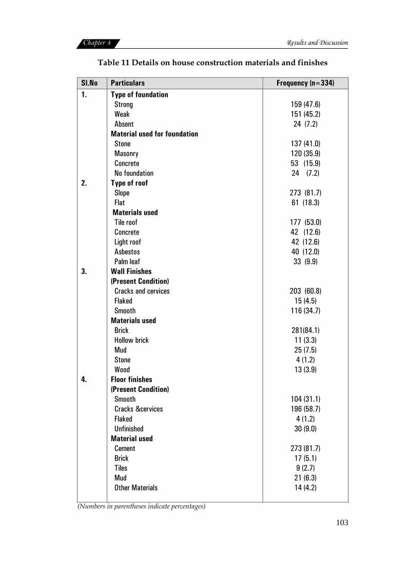
Table 11 Details on house construction materials and finishes
Sl.No Particulars Frequency (n=334) 1. 2. 3. 4.
Type of foundation Strong Weak Absent Material used for foundation Stone Masonry Concrete No foundation Type of roof Slope Flat Materials used Tile roof Concrete Light roof Asbestos Palm leaf Wall Finishes (Present Condition) Cracks and cervices Flaked Smooth Materials used Brick Hollow brick Mud Stone Wood Floor finishes (Present Condition) Smooth Cracks &cervices Flaked Unfinished Material used Cement Brick Tiles Mud Other Materials
159 (47.6) 151 (45.2) 24 (7.2)
137 (41.0) 120 (35.9) 53 (15.9) 24 (7.2)
273 (81.7) 61 (18.3)
177 (53.0) 42 (12.6) 42 (12.6) 40 (12.0) 33 (9.9)
203 (60.8) 15 (4.5)
116 (34.7)
281(84.1) 11 (3.3) 25 (7.5) 4 (1.2)
13 (3.9)
104 (31.1) 196 (58.7)
4 (1.2) 30 (9.0)
273 (81.7)
17 (5.1) 9 (2.7)
21 (6.3) 14 (4.2)
(Numbers in parentheses indicate percentages)
Chapter 4 Results and Discussion
104
Foundation
Foundation is said to be the base of any strong building, strength of
the foundation depends on the depth and material used. Majority of the
houses (47.6%) were found to have strong foundations. But there were
also few houses (7.2%) seen without foundation.
Materials commonly used for foundation were stone, concrete and
masonry works. Stone the strongest material for foundation was used in
41 percent of houses. Masonry was also used as an alternate for stone by
35.9 percent. Concrete was preferred by 15.9 percent.
Roof
Roof is an important feature for any building. The roof shape
usually are of two types, of which slope roof was used in majority (81.7%),
of houses in the slums. But 18.3 percent of houses had flat roofs also.
The material used for roof construction by almost half (53.0%) of
the sample was tiles, while the second preference went for light roofing
(12.6%), and concrete (12.6%) roofing. Asbestos (12.0%) was also preferred
by quite a few sample. Census of India (2001) data profile of Kerala
showed that tiles (50.2%) and concrete (38.2%) were mostly used as
roofing materials.
Wall
Appearance of wall depicted that though it was plastered, there
were cracks with cervices (60.8%) all over. Smooth finished walls were
also present (34.7%) in the slum houses.
Chapter 4 Results and Discussion
105
Materials used for constructing walls were bricks for 84.1 percent of
the households, mud (7.5%) and wooden planks (3.9%). In some houses
stone was used (1.2%), hollow bricks was also observed in 3.3 percent of
slum houses. Census of India (2001) reported that brick and stone were the
common materials for construction of walls in Kerala.
Floor
Floors were also mostly (58.7%) cracked with cervices. Smooth
floors were found only in 31.1 percent of houses, while flaked (1.2%) and
unfinished surfaces (9.0%) were also observed. NSSO (2002) states that
eleven out of hundred houses in urban areas are in bad condition and
required immediate major repair.
Different materials for floor finish are available in the market today.
Of these cement was the most preferred material by majority (81.7%) of
the slum residents. Mud was used by 6.3 percent, next preference was for
brick by 5.1 percent. Other material like sheets, and wooden planks etc
were laid in 4.2 percent of houses. The least used material was floor tiles
(2.7%). Preference for cement in Kerala, as a material for floor finish, was
also reported by Census of India (2001).
Prevailing conditions of houses
Prevailing conditions of roof, wall and floor, along with details on
dampness, lighting and ventilation was analyzed and given in the table
below.

Chapter 4 Results and Discussion
106
Table 12 Details on prevailing housing status
Sl.No Particulars Frequency (n=334)
1.
2.
3.
4.
5.
6.
Roof
Strong
Weak
Wall
Strong
Weak
Dampness
Water stagnation inside the house
Dampness
Floor
Strong
Weak
Ventilation
Adequate
Inadequate
Lighting
Adequate
Inadequate
219 (65.6)
115 (34.4)
116 (34.7)
218 (65.3)
191 (57.2)
210 (62.9)
104 (31.1)
230 (68.9)
157 (47.0)
177 (53.0)
53 (15.9)
281 (84.1)
(Numbers in parentheses indicate percentages)
The roof of 65.6 percent of the houses was found to be strong
whereas 34.4 percent of the houses had weak roof. Similarly the conditions
of wall were also not up to the mark 65.3 percent of the houses had walls
with cracks and flakes, and unfinished walls were also common.
Since most of the houses are located in the unhygienic environment,
mostly low lying areas, and the chances of water stagnation is more,
which was quite evident in the present study (57.2%). Heavy rain, poor
condition of roofs and walls, all are responsible for the dampness within
the house (62.9%).
Chapter 4 Results and Discussion
107
Lighting (84.1%) and ventilation (53.0%) was also inadequate in
most of the dwellings. Ventilation was generally the extent to which the
rooms were open to air and light (NSSO, 2004).
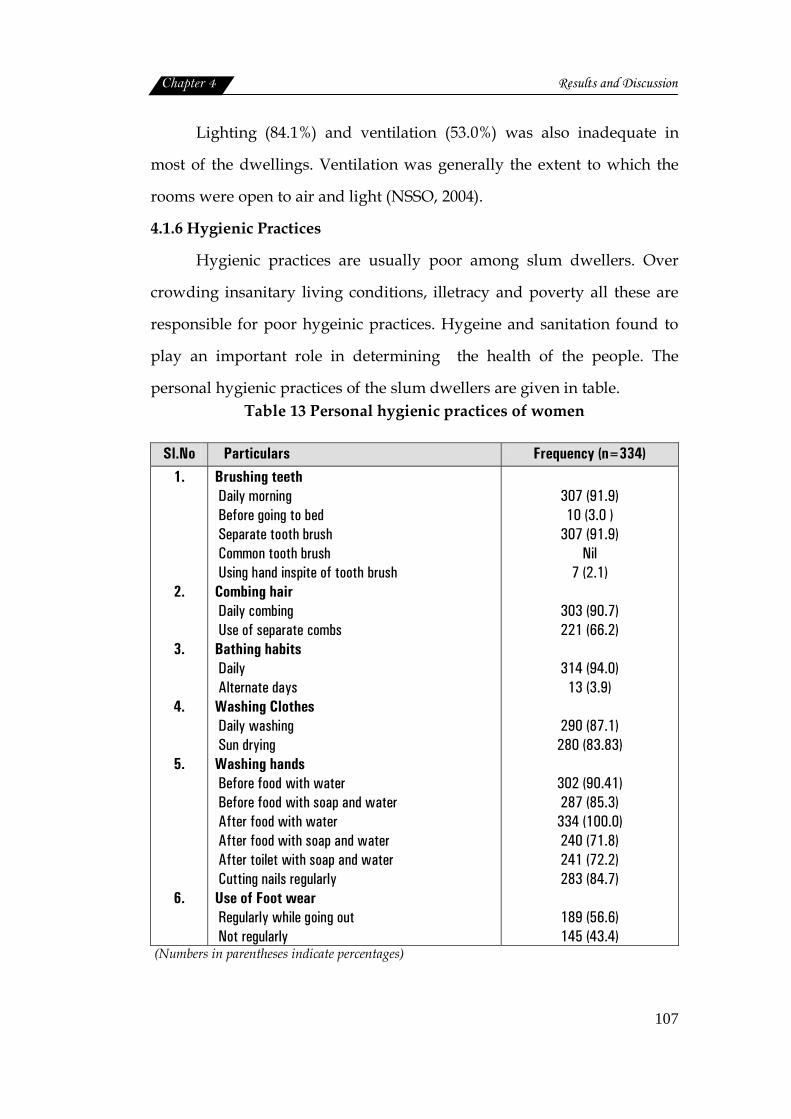
4.1.6 Hygienic Practices
Hygienic practices are usually poor among slum dwellers. Over
crowding insanitary living conditions, illetracy and poverty all these are
responsible for poor hygeinic practices. Hygeine and sanitation found to
play an important role in determining the health of the people. The
personal hygienic practices of the slum dwellers are given in table. Table 13 Personal hygienic practices of women
Sl.No Particulars Frequency (n=334) 1.
2.
3.
4.
5.
6.
Brushing teeth Daily morning Before going to bed Separate tooth brush Common tooth brush Using hand inspite of tooth brush Combing hair Daily combing Use of separate combs Bathing habits Daily Alternate days Washing Clothes Daily washing Sun drying Washing hands Before food with water Before food with soap and water After food with water After food with soap and water After toilet with soap and water Cutting nails regularly Use of Foot wear Regularly while going out Not regularly
307 (91.9) 10 (3.0 )
307 (91.9) Nil
7 (2.1)
303 (90.7) 221 (66.2)
314 (94.0)
13 (3.9)
290 (87.1) 280 (83.83)
302 (90.41) 287 (85.3) 334 (100.0) 240 (71.8) 241 (72.2) 283 (84.7)
189 (56.6) 145 (43.4)
(Numbers in parentheses indicate percentages)
Chapter 4 Results and Discussion
108
Poor personal hygiene was observed in a study by Muoki et al.
(2008). Brushing the teeth once daily in the morning was practiced by 91.9
percent of the sample. Brushing teeth twice a day, morning and before
going to bed was followed by only 3 percent of sample. Combing hair
daily was the habit of 90.7 percent of the sample but only 66.2 percent
used separate combs.
The habit of bathing daily was observed among 94.0 percent of
sample. Only very few (3.9%) bathed on alternate days. Clothes were
washed daily (87.1%) and sun dried (83.8%).
Even though majority of sample washed hands before food
(90.41%), use of soap and water for washing hands was observed among
85.3 percent. All washed their hands after food (100%), but the use of soap
was observed only among 71.8 percent. Washing with soap and water
after toilet was practised by 72.2 percent of the sample. Regular cutting of
nails (84.7%) was also observed among families.
Regular use of foot wear was found to be less common among slum
dwellers (56.6%), rest of them used only occasionally. Poor personal
hygiene among slum population was also reported by Muoki et al. (2008).
According to Nath (2003) personal and domestic hygienic practices cannot
be improved without improving basic amenities, such as water supply,
waste water disposal, solid waste management and the problems of
human settlements.
Chapter 4 Results and Discussion
109
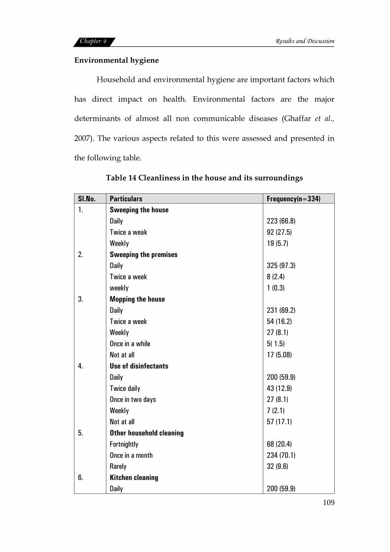
Environmental hygiene
Household and environmental hygiene are important factors which
has direct impact on health. Environmental factors are the major
determinants of almost all non communicable diseases (Ghaffar et al.,
2007). The various aspects related to this were assessed and presented in
the following table.
Table 14 Cleanliness in the house and its surroundings
Sl.No. Particulars Frequency(n=334) 1. 2. 3. 4. 5. 6.
Sweeping the house Daily Twice a weak Weekly Sweeping the premises Daily Twice a week weekly Mopping the house Daily Twice a week Weekly Once in a while Not at all Use of disinfectants Daily Twice daily Once in two days Weekly Not at all Other household cleaning Fortnightly Once in a month Rarely Kitchen cleaning Daily
223 (66.8) 92 (27.5) 19 (5.7) 325 (97.3) 8 (2.4) 1 (0.3) 231 (69.2) 54 (16.2) 27 (8.1) 5( 1.5) 17 (5.08) 200 (59.9) 43 (12.9) 27 (8.1) 7 (2.1) 57 (17.1) 68 (20.4) 234 (70.1) 32 (9.6) 200 (59.9)
Chapter 4 Results and Discussion
110
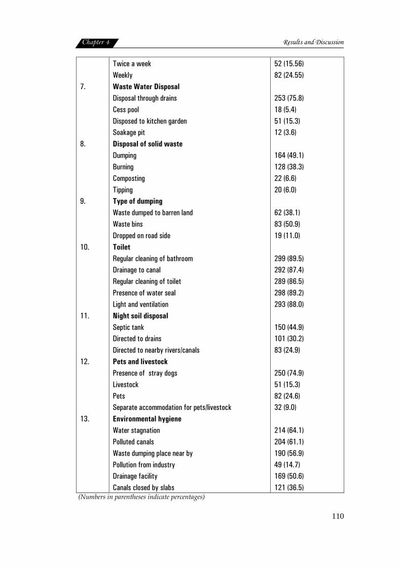
7. 8. 9. 10. 11. 12. 13.
Twice a week Weekly Waste Water Disposal Disposal through drains Cess pool Disposed to kitchen garden Soakage pit Disposal of solid waste Dumping Burning Composting Tipping Type of dumping Waste dumped to barren land Waste bins Dropped on road side Toilet Regular cleaning of bathroom Drainage to canal Regular cleaning of toilet Presence of water seal Light and ventilation Night soil disposal Septic tank Directed to drains Directed to nearby rivers/canals Pets and livestock Presence of stray dogs Livestock Pets Separate accommodation for pets/livestock Environmental hygiene Water stagnation Polluted canals Waste dumping place near by Pollution from industry Drainage facility Canals closed by slabs
52 (15.56) 82 (24.55) 253 (75.8) 18 (5.4) 51 (15.3) 12 (3.6) 164 (49.1) 128 (38.3) 22 (6.6) 20 (6.0) 62 (38.1) 83 (50.9) 19 (11.0) 299 (89.5) 292 (87.4) 289 (86.5) 298 (89.2) 293 (88.0) 150 (44.9) 101 (30.2) 83 (24.9) 250 (74.9) 51 (15.3) 82 (24.6) 32 (9.0) 214 (64.1) 204 (61.1) 190 (56.9) 49 (14.7) 169 (50.6) 121 (36.5)
(Numbers in parentheses indicate percentages)
Chapter 4 Results and Discussion
111
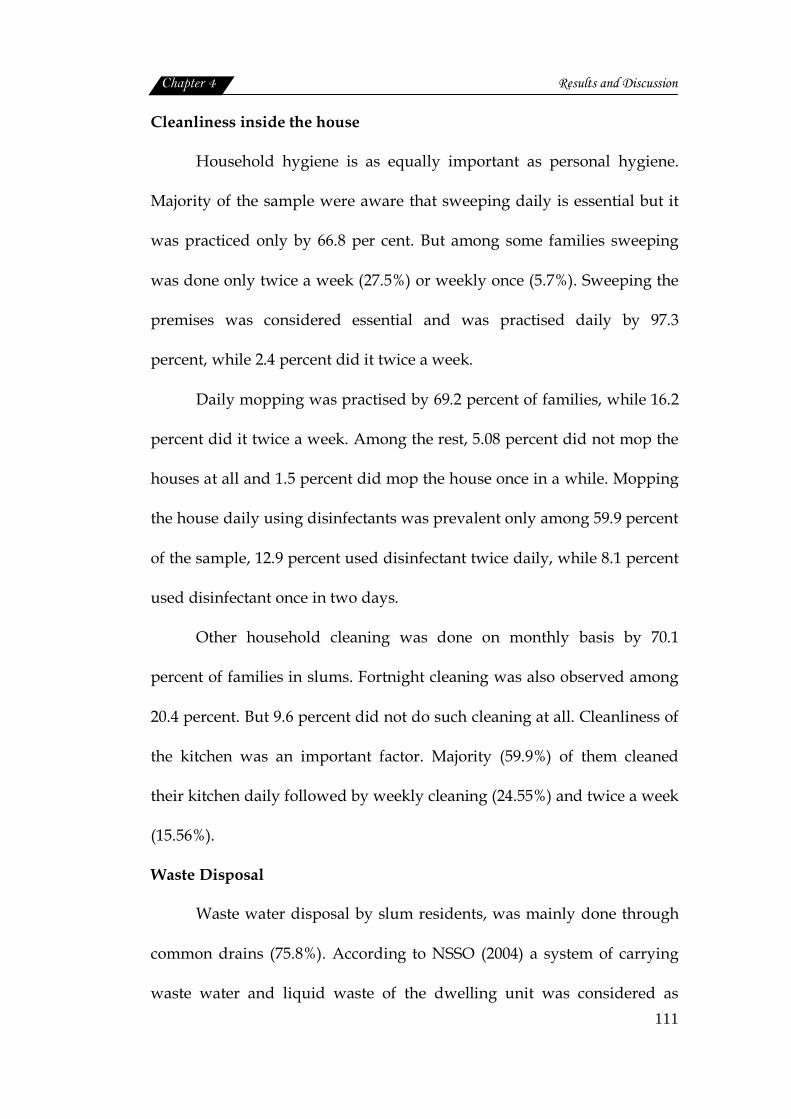
Cleanliness inside the house
Household hygiene is as equally important as personal hygiene.
Majority of the sample were aware that sweeping daily is essential but it
was practiced only by 66.8 per cent. But among some families sweeping
was done only twice a week (27.5%) or weekly once (5.7%). Sweeping the
premises was considered essential and was practised daily by 97.3
percent, while 2.4 percent did it twice a week.
Daily mopping was practised by 69.2 percent of families, while 16.2
percent did it twice a week. Among the rest, 5.08 percent did not mop the
houses at all and 1.5 percent did mop the house once in a while. Mopping
the house daily using disinfectants was prevalent only among 59.9 percent
of the sample, 12.9 percent used disinfectant twice daily, while 8.1 percent
used disinfectant once in two days.
Other household cleaning was done on monthly basis by 70.1
percent of families in slums. Fortnight cleaning was also observed among
20.4 percent. But 9.6 percent did not do such cleaning at all. Cleanliness of
the kitchen was an important factor. Majority (59.9%) of them cleaned
their kitchen daily followed by weekly cleaning (24.55%) and twice a week
(15.56%).
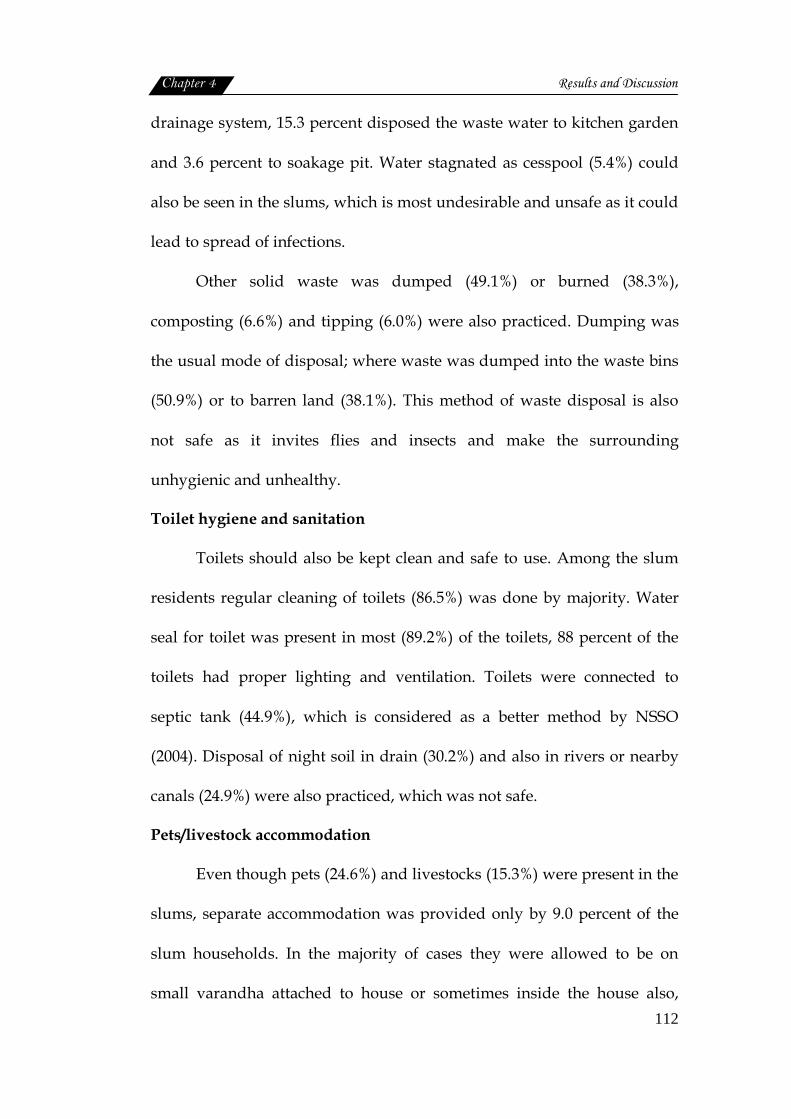
Waste Disposal
Waste water disposal by slum residents, was mainly done through
common drains (75.8%). According to NSSO (2004) a system of carrying
waste water and liquid waste of the dwelling unit was considered as
Chapter 4 Results and Discussion
112
drainage system, 15.3 percent disposed the waste water to kitchen garden
and 3.6 percent to soakage pit. Water stagnated as cesspool (5.4%) could
also be seen in the slums, which is most undesirable and unsafe as it could
lead to spread of infections.
Other solid waste was dumped (49.1%) or burned (38.3%),
composting (6.6%) and tipping (6.0%) were also practiced. Dumping was
the usual mode of disposal; where waste was dumped into the waste bins
(50.9%) or to barren land (38.1%). This method of waste disposal is also
not safe as it invites flies and insects and make the surrounding
unhygienic and unhealthy.
Toilet hygiene and sanitation
Toilets should also be kept clean and safe to use. Among the slum
residents regular cleaning of toilets (86.5%) was done by majority. Water
seal for toilet was present in most (89.2%) of the toilets, 88 percent of the
toilets had proper lighting and ventilation. Toilets were connected to
septic tank (44.9%), which is considered as a better method by NSSO
(2004). Disposal of night soil in drain (30.2%) and also in rivers or nearby
canals (24.9%) were also practiced, which was not safe.
Pets/livestock accommodation
Even though pets (24.6%) and livestocks (15.3%) were present in the
slums, separate accommodation was provided only by 9.0 percent of the
slum households. In the majority of cases they were allowed to be on
small varandha attached to house or sometimes inside the house also,
Chapter 4 Results and Discussion
113
which could be considered as a most unhygienic practice. As Nath (2003)
pointed out inadequacy of housing in most urban poor invariably leads to
poor home hygiene.
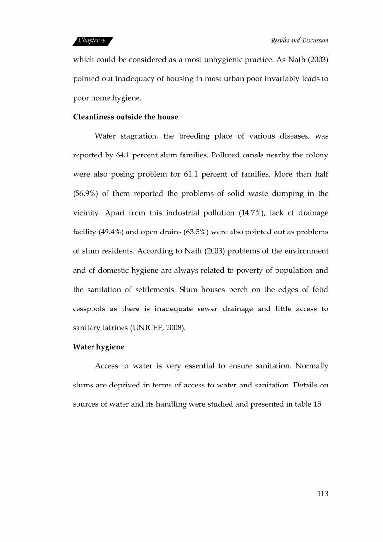
Cleanliness outside the house
Water stagnation, the breeding place of various diseases, was
reported by 64.1 percent slum families. Polluted canals nearby the colony
were also posing problem for 61.1 percent of families. More than half
(56.9%) of them reported the problems of solid waste dumping in the
vicinity. Apart from this industrial pollution (14.7%), lack of drainage
facility (49.4%) and open drains (63.5%) were also pointed out as problems
of slum residents. According to Nath (2003) problems of the environment
and of domestic hygiene are always related to poverty of population and
the sanitation of settlements. Slum houses perch on the edges of fetid
cesspools as there is inadequate sewer drainage and little access to
sanitary latrines (UNICEF, 2008).
Water hygiene
Access to water is very essential to ensure sanitation. Normally
slums are deprived in terms of access to water and sanitation. Details on
sources of water and its handling were studied and presented in table 15.
Chapter 4 Results and Discussion
114
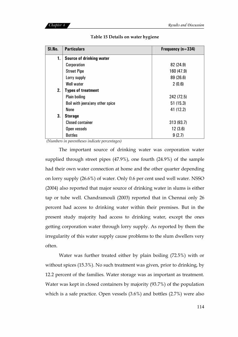
Table 15 Details on water hygiene
Sl.No. Particulars Frequency (n=334)
1.
2.
3.
Source of drinking water Corporation Street Pipe Lorry supply Well water Types of treatment Plain boiling Boil with jeera/any other spice None Storage Closed container Open vessels Bottles
82 (24.9)
160 (47.9) 89 (26.6)
2 (0.6)
242 (72.5) 51 (15.3) 41 (12.2)
313 (93.7)
12 (3.6) 9 (2.7)
(Numbers in parentheses indicate percentages)
The important source of drinking water was corporation water
supplied through street pipes (47.9%), one fourth (24.9%) of the sample
had their own water connection at home and the other quarter depending
on lorry supply (26.6%) of water. Only 0.6 per cent used well water. NSSO
(2004) also reported that major source of drinking water in slums is either
tap or tube well. Chandramouli (2003) reported that in Chennai only 26
percent had access to drinking water within their premises. But in the
present study majority had access to drinking water, except the ones
getting corporation water through lorry supply. As reported by them the
irregularity of this water supply cause problems to the slum dwellers very
often.
Water was further treated either by plain boiling (72.5%) with or
without spices (15.3%). No such treatment was given, prior to drinking, by
12.2 percent of the families. Water storage was as important as treatment.
Water was kept in closed containers by majority (93.7%) of the population
which is a safe practice. Open vessels (3.6%) and bottles (2.7%) were also

Chapter 4 Results and Discussion
115
used. Household water treatment and safe storage (HWTS) interventions
can lead to dramatic improvements in drinking water quality and
reductions in diarrhoeal disease (WHO, 2010).
Food Hygiene and related practices
Food hygiene and related practices are based on the knowledge and
awareness of the sample on these aspects. Various factors related to this,
about which the women were aware of and practiced in the day to day
life, are obtained and given in table 16.
Table 16 Food hygiene and related practices
Sl.No Particulars Frequency (n=334) 1.
2. 3. 4. 5. 6. 7. 8. 9. 10. 11. 12. 13.
14. 15. 16. 17. 18. 19. 20. 21. 22. 23. 24. 25.
Seasonal foods are more nutritious Food Purchased from roadside is not hygienic Fresh food is more nutritious Packed food is more safe Sun drying of cereals and pulses improves storage quality Proper storage prevents food spoilage by pests Food containers should be washed and sun dried Vegetable should be washed before storing Leafy vegetables could be stored in moist cloth Fly proof cover prevent infection Vegetable should be washed before cutting Vegetable must be cut into large pieces Food must be cooked with adequate water to preserve nutrients Throwing stock depletes nutrients Vessels should be covered during cooking Adding of soda destroys nutrients Iron vessels increase the iron content Absorption method prevent nutrient loss Reheating of food depletes nutrients Food should be kept closed before serving Serving vessels should be clean Food should be served in clean surroundings Spoon feeding for children is better than hand feeding Tying of hair during cooking is hygienic Washing hands before cooking is hygienic
182 (54.5) 130 (38.9) 274 (82.0) 180 (53.9) 68 (20.4) 208 (62.3) 273 (81.7) 122 (36.5) 54 (16.2) 145 (73.7) 293 (87.7) 141 (42.2) 254 (76.0)
225 (67.4) 301 (90.1) 106 (31.7) 95 (28.4) 143 (72.2)
32 (9.6) 320 (95.8) 319 (95.5) 282 (84.4) 79 (23.7) 310 (92.8) 311 (92.5)
(Numbers in parentheses indicate percentages)
Chapter 4 Results and Discussion
116
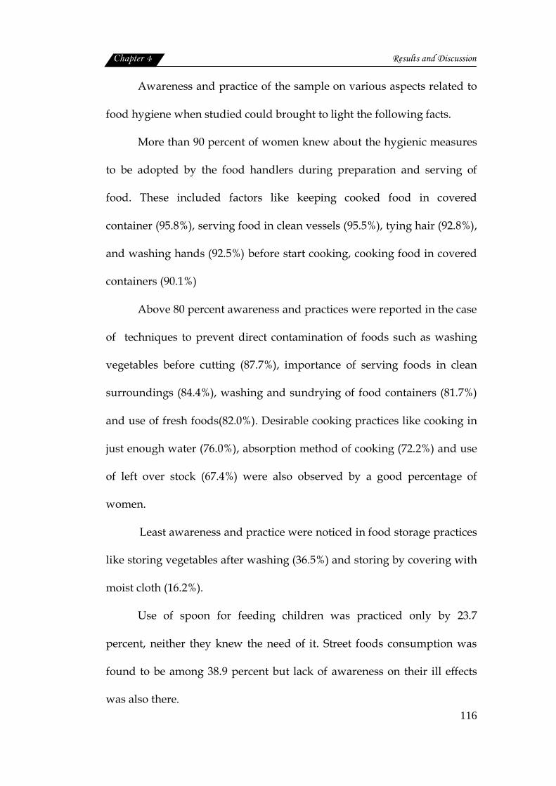
Awareness and practice of the sample on various aspects related to
food hygiene when studied could brought to light the following facts.
More than 90 percent of women knew about the hygienic measures
to be adopted by the food handlers during preparation and serving of
food. These included factors like keeping cooked food in covered
container (95.8%), serving food in clean vessels (95.5%), tying hair (92.8%),
and washing hands (92.5%) before start cooking, cooking food in covered
containers (90.1%)
Above 80 percent awareness and practices were reported in the case
of techniques to prevent direct contamination of foods such as washing
vegetables before cutting (87.7%), importance of serving foods in clean
surroundings (84.4%), washing and sundrying of food containers (81.7%)
and use of fresh foods(82.0%). Desirable cooking practices like cooking in
just enough water (76.0%), absorption method of cooking (72.2%) and use
of left over stock (67.4%) were also observed by a good percentage of
women.
Least awareness and practice were noticed in food storage practices
like storing vegetables after washing (36.5%) and storing by covering with
moist cloth (16.2%).
Use of spoon for feeding children was practiced only by 23.7
percent, neither they knew the need of it. Street foods consumption was
found to be among 38.9 percent but lack of awareness on their ill effects
was also there.

Chapter 4 Results and Discussion
117
In short women at slums had better awareness and practice on food
hygiene aspects particularly during cooking and serving food. Desirable
food preparation techniques to conserve nutrients were also followed to
an appreciable extent. The gap was mainly on food storage practices and
feeding of young children. Street food consumption and techniques to
improve the nutritional value of available foods.
Availability and use of public utilities
Availability of basic services with special reference to its utility was
studied. The basic services include electrification, drinking water,
transport, educational, medical, and marketing and recreation. The details
are presented in table 17.
Table 17 Availability and use of basic services
Sl .No. Particulars Availability (n=334)
Usage (n=334)
1.
2.
3.
4.
Electrification
Present
Absent
Street Light
Present
Absent
Drinking water
Corporation
Public tap
Lorry supply
Road
Walkable
Very near
Very far
297(88.9)
37(11.1)
279(83.5)
55 (16.5)
82(24.9)
160(47.9)
89(26.6)
258(77.2)
64(19.2)
12(3.6)
297 (88.9)
Nil
279 (83.5)
Nil
82 (24.9)
160 (47.9)
89 (26.6)
258 (77.2)
64 (19.2)
12 (3.6)

Chapter 4 Results and Discussion
118
5.
6.
7.
8.
9.
Transport
Available
Not available
Education
Preschool
Creche
Primary School
High School
Higher Secondary School
College
Medical Facilities
Govt .Hospitals
Private
Homeo
Ayurvedha
Marketing
Ration Shop
Market place
Vegetable shops
Medical shop
Bakery
Hotel
Post Office
Bank
Recreation
Movie house
Park
Reading room
Play ground
175(52.4)
159(47.6)
332(99.4)
17(5.1)
209(62.57)
126(37.72)
143(42.81)
243(72.8)
157(47.0)
67(20.1)
92(27.6)
18(5.4)
228(68.3)
264(79.0)
287(85.9)
210(62.9)
221(66.2)
207(62.0)
147(44.0)
106(31.7)
75(22.5)
93(27.8)
35(10.5)
19(5.7)
175 (52.4)
Nil
312 (96.4)
6 (0.9)
285 (85.32)
156 (46.7)
17 (5.1)
7 (2.1)
248 (74.25)*
45 (13.47)
30 (8.98)
11 (3.3)
254 (76.04)*
314 (94.01)*
320 (95.8)*
220 (65.86)*
43 (12.9)
33 (9.9)
147 (44.0)
44 (13.2)
71 (21.3)
76 (22.8)
8 (2.4)
15 (4.5)
(Numbers in parentheses indicate percentages) *Not available near slums, but use this services wherever available
Chapter 4 Results and Discussion
119
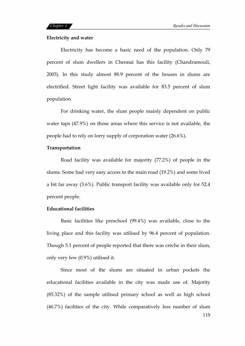
Electricity and water
Electricity has become a basic need of the population. Only 79
percent of slum dwellers in Chennai has this facility (Chandramouli,
2003). In this study almost 88.9 percent of the houses in slums are
electrified. Street light facility was available for 83.5 percent of slum
population
For drinking water, the slum people mainly dependent on public
water taps (47.9%) on those areas where this service is not available, the
people had to rely on lorry supply of corporation water (26.6%).
Transportation
Road facility was available for majority (77.2%) of people in the
slums. Some had very easy access to the main road (19.2%) and some lived
a bit far away (3.6%). Public transport facility was available only for 52.4
percent people.
Educational facilities
Basic facilities like preschool (99.4%) was available, close to the
living place and this facility was utilised by 96.4 percent of population.
Though 5.1 percent of people reported that there was crèche in their slum,
only very few (0.9%) utilised it.
Since most of the slums are situated in urban pockets the
educational facilities available in the city was made use of. Majority
(85.32%) of the sample utilised primary school as well as high school
(46.7%) facilities of the city. While comparatively less number of slum
Chapter 4 Results and Discussion
120
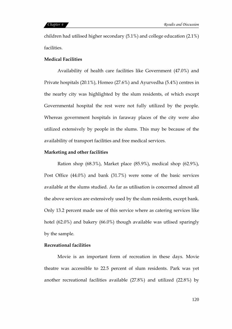
children had utilised higher secondary (5.1%) and college education (2.1%)
facilities.
Medical Facilities
Availability of health care facilities like Government (47.0%) and
Private hospitals (20.1%), Homeo (27.6%) and Ayurvedha (5.4%) centres in
the nearby city was highlighted by the slum residents, of which except
Governmental hospital the rest were not fully utilized by the people.
Whereas government hospitals in faraway places of the city were also
utilized extensively by people in the slums. This may be because of the
availability of transport facilities and free medical services.
Marketing and other facilities
Ration shop (68.3%), Market place (85.9%), medical shop (62.9%),
Post Office (44.0%) and bank (31.7%) were some of the basic services
available at the slums studied. As far as utilisation is concerned almost all
the above services are extensively used by the slum residents, except bank.
Only 13.2 percent made use of this service where as catering services like
hotel (62.0%) and bakery (66.0%) though available was utlised sparingly
by the sample.
Recreational facilities
Movie is an important form of recreation in these days. Movie
theatre was accessible to 22.5 percent of slum residents. Park was yet
another recreational facilities available (27.8%) and utilized (22.8%) by
Chapter 4 Results and Discussion
121
people. Regarding the reading room and play ground the availability as
well as usage were very limited.
4.2. Nutritional and Health Status of Women
Women's health and nutritional status is inextricably bound with
social, cultural, and economic factors that influence all aspects of their
lives, and it has consequences not only on the women themselves but also
for the well-being of their children (World Bank Group, 1996).
4.2.1. Nutritional status of women
Nutritional status of women covers details like anthropometry,
biochemical, clinical and diet survey. The data procured on these lines are
analysed and discussed in the following sections.
4.2.1.1 Nutritional anthropometry
Nutritional anthropometry has been defined as ‘measurements of
the variations of the physical dimensions and the gross composition of the
human body at different age levels and degrees of nutrition’ (Jelliffe,
1966). The anthropometric measurements of women in terms of height,
weight and body mass index was used for the study. Waist-hip ratio of
women was also assessed. The data was systematically analyzed and
presented in the following tables.
Age wise distribution of sample
The distribution of the sample based on age is presented in table 18.
Chapter 4 Results and Discussion
122
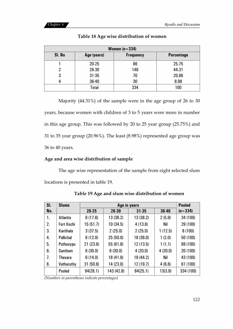
Table 18 Age wise distribution of women
Women (n=334) Sl. No Age (years) Frequency Percentage
1 2 3 4
20-25 26-30 31-35 36-40
86 148 70 30
25.75 44.31 20.96 8.98
Total 334 100
Majority (44.31%) of the sample were in the age group of 26 to 30
years, because women with children of 3 to 5 years were more in number
in this age group. This was followed by 20 to 25 year group (25.75%) and
31 to 35 year group (20.96%). The least (8.98%) represented age group was
36 to 40 years.
Age and area wise distribution of sample
The age wise representation of the sample from eight selected slum
locations is presented in table 19.
Table 19 Age and slum wise distribution of women
Age in years Sl. No.
Slums 20-25 26-30 31-35 36-40
Pooled (n=334)
1. 2. 3. 4. 5. 6. 7. 8.
Atlantis Fort Kochi Karithala Pallichal Puthuvypu Santhom Thevara Vathuruthy
6 (17.6) 15 (51.7) 3 (37.5) 6 (12.0)
21 (23.6) 6 (30.0) 6 (14.0)
31 (50.8)
13 (38.2) 10 (34.5) 2 (25.0) 25 (50.0) 55 (61.8) 6 (30.0) 18 (41.9) 14 (23.0)
13 (38.2) 4 (13.8) 2 (25.0)
18 (36.0) 12 (13.5) 4 (20.0)
19 (44.2) 12 (19.7)
2 (5.9) Nil
1 (12.5) 1 (2.0) 1 (1.1)
4 (20.0) Nil
4 (6.6)
34 (100) 29 (100) 8 (100) 50 (100) 89 (100) 20 (100) 43 (100) 61 (100)
Pooled 94(28.1) 143 (42.8) 84(25.1) 13(3.9) 334 (100) (Numbers in parentheses indicate percentages)

Chapter 4 Results and Discussion
123
Maximum number of sample (women) is from Puthuvypu slum (89)
followed by vathuruthy (61) and Pallichal (50) as these slums had
proportionately more number of women population. Age wise
distribution showed that maximum number of sample in the age group of
26 to 30 years were from Puthuvypu (61.8%) followed by Pallichal (50.0%)
and Thevara (41.9%) slums. Whereas younger age groups were mostly
from Fort Kochi (51.7%) Vathuruthy (50.8%) and Karithala (37.5%).
Thus it is obvious that representation of all age groups from all the
selected slums was included in the sample.
Mean height and weight
Mean height and weight of the sample were statistically analysed.
The standard values used for comparison are the 50th percentile values of
heights and weights specified by NCHS (1987). The results are presented
in the table below.
Table 20 Mean height of mothers in comparison with standard height®
Height(cm) Age
(yrs) Mean ±SD
Standard weight
Standard Error
Mean difference
‘t’ value
‘p’value
20-25
26-30
31-35
36-40
152.7 ±0.0562
153.4±0.0599
153.3±0.0624
151.4±0.0721
163.3
162.8
162.8
162.8
0.00547
0.00477
0.00637
0.01803
-.1060 ( -6.49 )
-.0936(-5.77 )
-.0949(-5.83)
-.1136(-7.00)
-19.393
-19.649
-14.886
-6.303
0.000**
0.000**
0.000**
0.000**
Pooled 153.11 ±0.0600 162.92 0.00310 -.0981 -31.666 0.000**
®Ref: NCHS (1987) (Numbers in parentheses indicate percentage Deviation)
Chapter 4 Results and Discussion
124
36 - 4031 - 3526 - 3020 -25
Age
1.70
1.60
1.50
1.40
1.30
Heig
ht
371
167
34
84
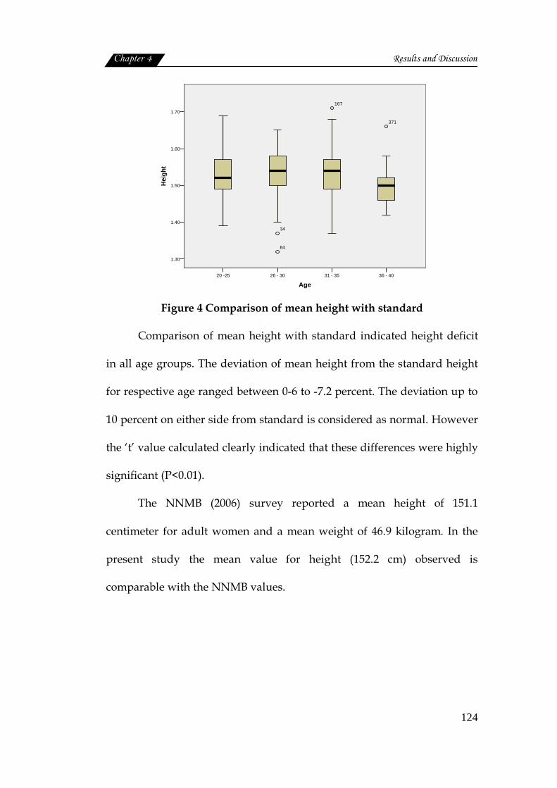
Figure 4 Comparison of mean height with standard
Comparison of mean height with standard indicated height deficit
in all age groups. The deviation of mean height from the standard height
for respective age ranged between 0-6 to -7.2 percent. The deviation up to
10 percent on either side from standard is considered as normal. However
the ‘t’ value calculated clearly indicated that these differences were highly
significant (P<0.01).
The NNMB (2006) survey reported a mean height of 151.1
centimeter for adult women and a mean weight of 46.9 kilogram. In the
present study the mean value for height (152.2 cm) observed is
comparable with the NNMB values.
Chapter 4 Results and Discussion
125
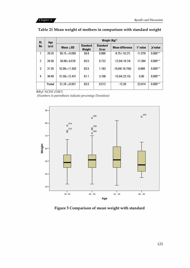
Table 21 Mean weight of mothers in comparison with standard weight
Weight (Kg)® Sl.No
Age (yrs) Mean ±SD Standard
Weight Standard
Error Mean difference ‘t’ value ‘p’value
1
2
3
4
20-25
26-30
31-35
36-40
50.15 ±9.059
50.96±9.076
52.86±11.593
51.56±12.431
59.9
63.5
63.5
67.1
0.880
0.722
1.183
3.108
-9.75 (-16.27)
-12.54(-19.74)
-10.64(-16.755)
-15.54(-23.15)
-11.079
-17.364
-8.989
-5.00
0.000**
0.000**
0.000**
0.000**
Pooled 51.24 ±9.937 63.5 0.512 -12.26 -23.914 0.000**
®Ref: NCHS (1987) (Numbers in parentheses indicate percentage Deviation)
36 - 4031 - 3526 - 3020 -25
Age
90
80
70
60
50
40
30
Wei
ght
105330
165
363
374
215
Figure 5 Comparison of mean weight with standard
Chapter 4 Results and Discussion
126
In the case of body weight also clear evidences of deficit ranged
from -16.27 percent to -23.15 percent was observed. The ‘t’ values
computed also revealed a highly significant difference (P<0.01) between
the observed and standard weight measurements of women. It indicated
chronic energy deficiency which was found to increase with the age.
The NNMB (2006) survey reported a mean weight for adult women
as 46.9 kilogram. While the present study observed a mean weight 51.2 Kg
is higher than the national average (46.9 Kg). Hence it can be stated that,
slum women of Kerala although suffer from chronic energy deficiency,
they are in a slightly better position when compared with Indian women.
Age and body mass index
Body mass index is considered as the most suitable, objective
anthropometric indicator of nutritional status of the adult (Shetty, 2005).
The body mass index of the sample based on age was categorized using
BMI classification given by James et al. (1988). The results are presented in
detail in the following table.
Chapter 4 Results and Discussion
127
Tabl
e 22
Age
and
BM
I Sta
tus
of w
omen
®Re
f: Ja
mes
et a
l. (1
988)
N
S-N
ot S
igni
fican
t (N
umbe
rs in
par
enth
eses
indi
cate
per
cent
ages
)
Chapter 4 Results and Discussion
128
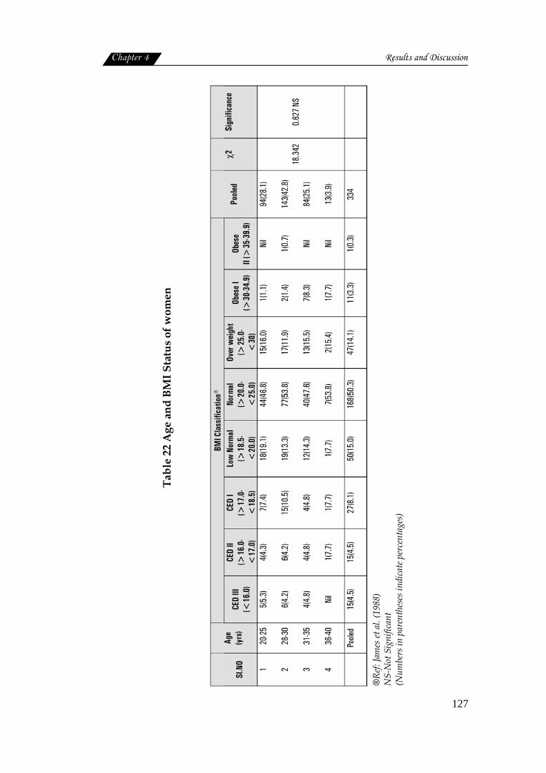
BMI classification of the sample showed that almost half of the
population (50.3%) had normal BMI. most of women with normal BMI
belonged to 26 to 30 years and 36 to 40 years, This was followed by the
low normal sample (15.0%).
The number of sample seemed to reduce, as BMI status moved
towards either side of the normal states, such as overweight and obesity
and the stages of chronic energy deficiency.
Low normal was found more among youngest age group of 20 to 25
years (19.1%) and less among 36 to 40 years (7.7%). Chronic energy
deficiency was more among middle aged women of 26 to 30 years. Over
weight and obesity were found to increase with age. Women of 31 to 35
years (8.3%) and 36 to 40 years (7.7%) were more affected than younger
age groups.
However, the above found differences in the BMI status of women
belonged to different age groups were not statistically significant,
indicating the fact that age has no binding on BMI status of women
residing in the slums.
Indian women are thinner and shorter than women in other parts of
Asia. This has consequences for their own health and that of their
children. India has one of the highest incidences of low birth weight in the
world (UNICEF, 2001). This is not simply because India is economically
poor; it has a higher gross national product than many other developing
countries and has shown remarkable economic growth in recent years.
Gender inequality, deeply entrenched in Indian society may be a factor
(Sen, 2001). Thinner women had thinner babies, and also that they were
significantly thinner than their husbands (Chorghade et al., 2006).
Slum locations and body mass index
Table 23 shows the association between body mass index of the
sample and the location of slums.

Chapter 4 Results and Discussion
129
Tabl
e 23
Slu
m lo
cati
ons
and
BMI s
tatu
s of
wom
en
(Numbers in parentheses indicate percentages)
NS‐Not Significant
®Ref: James et al. (1988)
CED: Chronic energy deficiency
Chapter 4 Results and Discussion
130
As the table depicts majority of slum women (50.3%) were classified
under normal BMI. More women from Puthuvypu (58.4%), Thevara
(55.8%) and Fort Kochi (51.7%) came under normal category. Over weight
and obese women were more in Vathuruthy (22.9%) and Atlantis (20.5%)
Puthuvypu (20.3%) slums. Whereas low normal weight and energy
deficiencies of varying degrees were observed more among Santhom
Pallichal and Atlantis slums.
Hence it can be inferred that no single unit of slum studied, could
be referred as having most of the women in undernourished or over
nourished category.
However, total absence of obesity in the slums of Fort Kochi,
Karithala and Thevara is something need special mention. Here also
statistical analysis failed to show any significant difference among slums
with respect to BMI status of women residing there.
NNMB (2006) reports that chronic energy deficiency was least in
Kerala (21.1%), while obesity was high (24.0%), when compared with other
states. This finding is not agreeable with women living in urban slums.
Socioeconomic status and body mass index
The socioeconomic status of the slum population is always less than
the other urban population. An attempt was made to compute the
socioeconomic status of the sample using socioeconomic scale by
Kuppuswamy (1981). The following table presents the details.
Chapter 4 Results and Discussion
131
Tabl
e 24
Soc
ioec
onom
ic s
tatu
s an
d BM
I sta
tus
of w
omen
(Numbers in parentheses indicate percentages)
NS‐Not Significant
®Ref: James et al. (1988)
CED: Chronic energy deficiency
Chapter 4 Results and Discussion
132
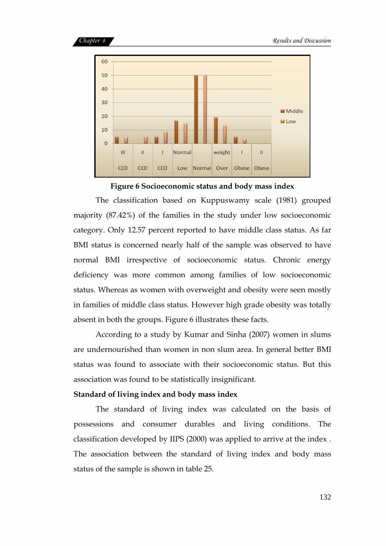
Figure 6 Socioeconomic status and body mass index
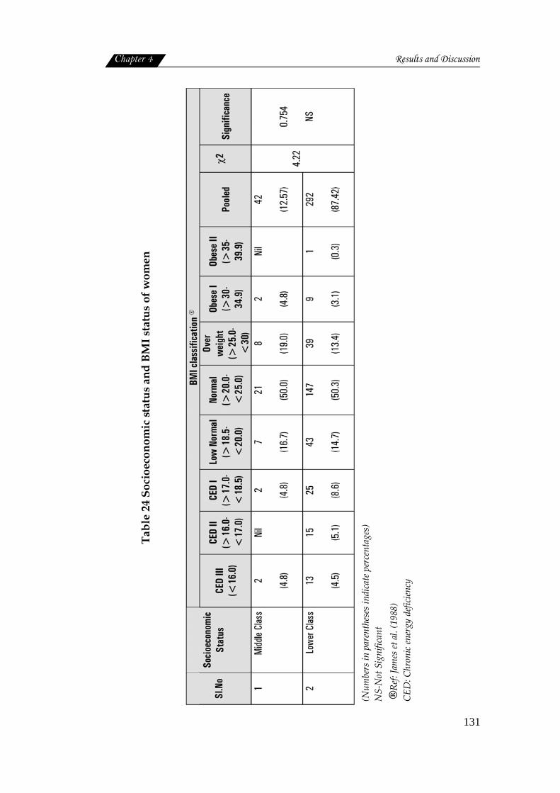
The classification based on Kuppuswamy scale (1981) grouped
majority (87.42%) of the families in the study under low socioeconomic
category. Only 12.57 percent reported to have middle class status. As far
BMI status is concerned nearly half of the sample was observed to have
normal BMI irrespective of socioeconomic status. Chronic energy
deficiency was more common among families of low socioeconomic
status. Whereas as women with overweight and obesity were seen mostly
in families of middle class status. However high grade obesity was totally
absent in both the groups. Figure 6 illustrates these facts.
According to a study by Kumar and Sinha (2007) women in slums
are undernourished than women in non slum area. In general better BMI
status was found to associate with their socioeconomic status. But this
association was found to be statistically insignificant.
Standard of living index and body mass index
The standard of living index was calculated on the basis of
possessions and consumer durables and living conditions. The
classification developed by IIPS (2000) was applied to arrive at the index .
The association between the standard of living index and body mass
status of the sample is shown in table 25.

Chapter 4 Results and Discussion
133
Tabl
e 25
Sta
ndar
d of
livi
ng in
dex
and
body
mas
s st
atus
of w
omen
®Ref: BMI James et al(1988)
NS‐Not significant
(Numbers in parentheses indicate percentages)
*CED –chronic energy deficiency
Chapter 4 Results and Discussion
134
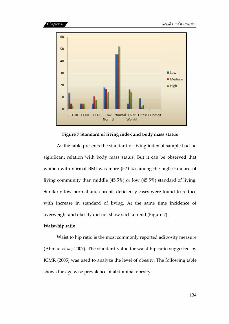
Figure 7 Standard of living index and body mass status
As the table presents the standard of living index of sample had no
significant relation with body mass status. But it can be observed that
women with normal BMI was more (52.0%) among the high standard of
living community than middle (45.5%) or low (45.5%) standard of living.
Similarly low normal and chronic deficiency cases were found to reduce
with increase in standard of living. At the same time incidence of
overweight and obesity did not show such a trend (Figure.7).
Waist-hip ratio
Waist to hip ratio is the most commonly reported adiposity measure
(Ahmad et al., 2007). The standard value for waist-hip ratio suggested by
ICMR (2005) was used to analyze the level of obesity. The following table
shows the age wise prevalence of abdominal obesity.
Chapter 4 Results and Discussion
135
Table 26 Age and waist‐hip ratio of women
Waist -hip ratio® Sl. No.
Age (yrs) Normal
(< 0.8) Abdominal
Obesity ( ≥0.8) Pooled
χ2
Significance
1.
2.
3.
4.
20-25
26-30
31-35
36-40
8(8.5)
13(9.1)
5(6.0)
1(7.7)
86(91.5)
130(90.9)
79(94.0)
12(92.3)
94
143
84
13
0.735 0.865
NS
Pooled 27(8.1) 307(91.9) 334
®Ref : ICMR ,2005
NS-Not significant
0
10
20
30
40
50
60
70
80
90
100
20-25 26-30 31-35 36-40
Normal
AbdominalObesity
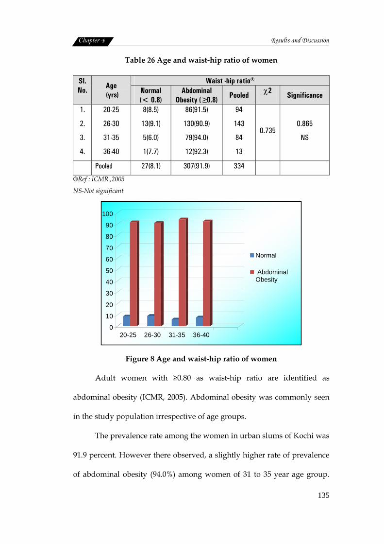
Figure 8 Age and waist-hip ratio of women
Adult women with ≥0.80 as waist-hip ratio are identified as
abdominal obesity (ICMR, 2005). Abdominal obesity was commonly seen
in the study population irrespective of age groups.
The prevalence rate among the women in urban slums of Kochi was
91.9 percent. However there observed, a slightly higher rate of prevalence
of abdominal obesity (94.0%) among women of 31 to 35 year age group.
Chapter 4 Results and Discussion
136
NNMB (2006) also reported the highest prevalence of waist-hip ratio
(91.8%) among women of Kerala; which is in accordance to the findings of
the present study. Figure 8 presents the waist-hip ratio of the sample
studied. But the statistical analysis to find out the association between age
and waist-hip of women could not show any significant relation between
these two factors.
Slum locations and waist-hip ratio
Chi square analysis was employed to find the association between
slum locations and waist hip ratio of the sample. The results are presented
in the following table.
Table 27 Slum locations and waist-hip ratio of women
Waist-hip ratio Sl.No. Slums Normal
(< 0.8) Abdominal
Obesity ( ≥0.8)
Pooled
χ2
Significance
1.
2.
3.
4.
5.
6.
7.
8.
Atlantis
Fort Kochi
Karithala
Pallichal
Puthuvypu
Santhom
Thevara
Vathuruthy
5 (14.7)
1(3.4)
Nil
1(2.0)
14(15.7)
1(5.0)
3(7.0)
2(3.3)
29(85.3)
28(96.6)
8(100.0)
49(98.0)
75(84.3)
19(95.0)
40(93.0)
59(96.7)
34
29
8
50
89
20
43
61
15.265 0.033*
Pooled 27(8.1) 307(91.9) 334
(Numbers in parentheses indicate percentages)
*significant at 5% level
Chapter 4 Results and Discussion
137
Slum wise distribution of the sample indicated that incidence of
abdominal obesity was more among women of Karithala (100%) Pallichal
(98.0%) Vathuruthy (96.7%) and Fort Kochi (96.6%) slums. In NFHS-3
reports (2006) also it was mentioned that among Indian women
prevalence of overweight and obesity are on rise.
The statistical analysis of waist-hip ratio of women among slum
showed that there existed a significant relation (P<0.05) between the
locations of slums and obesity.
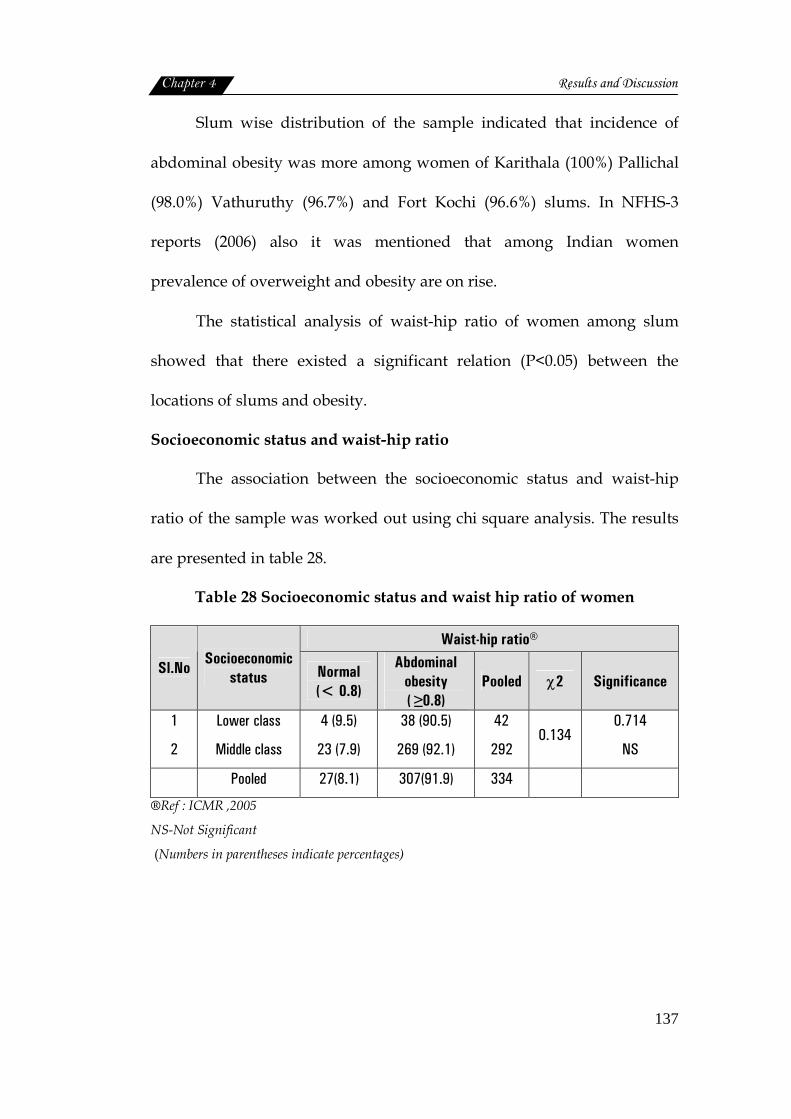
Socioeconomic status and waist-hip ratio
The association between the socioeconomic status and waist-hip
ratio of the sample was worked out using chi square analysis. The results
are presented in table 28.
Table 28 Socioeconomic status and waist hip ratio of women
Waist-hip ratio®
Sl.No Socioeconomic
status Normal (< 0.8)
Abdominal obesity ( ≥0.8)
Pooled χ2 Significance
1
2
Lower class
Middle class
4 (9.5)
23 (7.9)
38 (90.5)
269 (92.1)
42
292 0.134
0.714
NS
Pooled 27(8.1) 307(91.9) 334
®Ref : ICMR ,2005
NS-Not Significant
(Numbers in parentheses indicate percentages)
Chapter 4 Results and Discussion
138
0
1020
3040
5060
7080
90100
Lower class Middle class
Normal (< 0.8)
Abdominal obesity(?0.8)
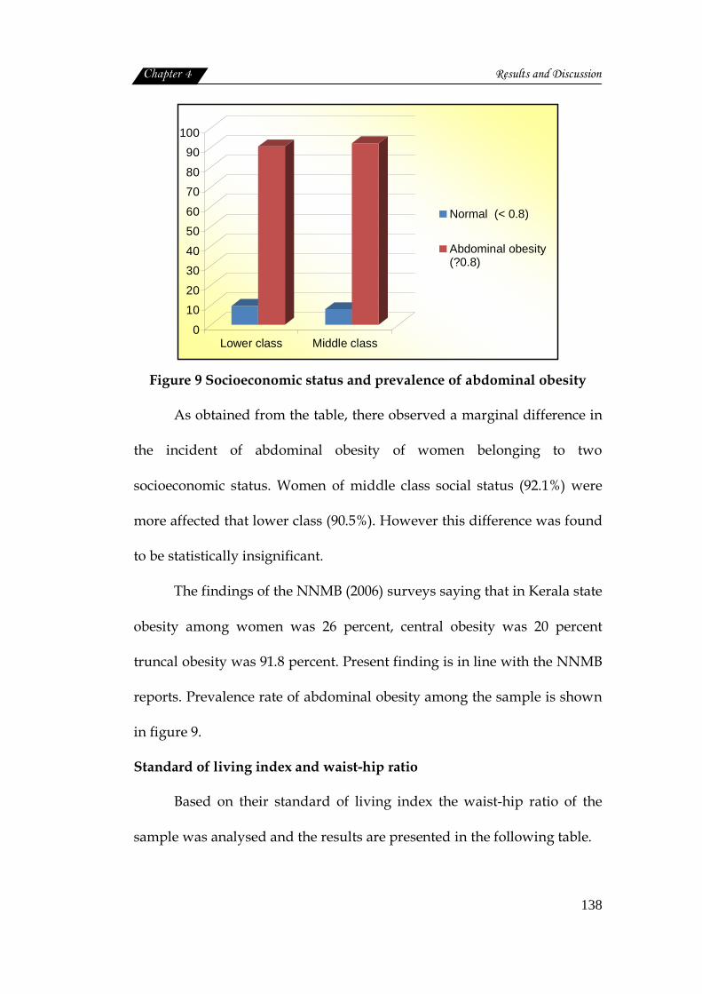
Figure 9 Socioeconomic status and prevalence of abdominal obesity
As obtained from the table, there observed a marginal difference in
the incident of abdominal obesity of women belonging to two
socioeconomic status. Women of middle class social status (92.1%) were
more affected that lower class (90.5%). However this difference was found
to be statistically insignificant.
The findings of the NNMB (2006) surveys saying that in Kerala state
obesity among women was 26 percent, central obesity was 20 percent
truncal obesity was 91.8 percent. Present finding is in line with the NNMB
reports. Prevalence rate of abdominal obesity among the sample is shown
in figure 9.
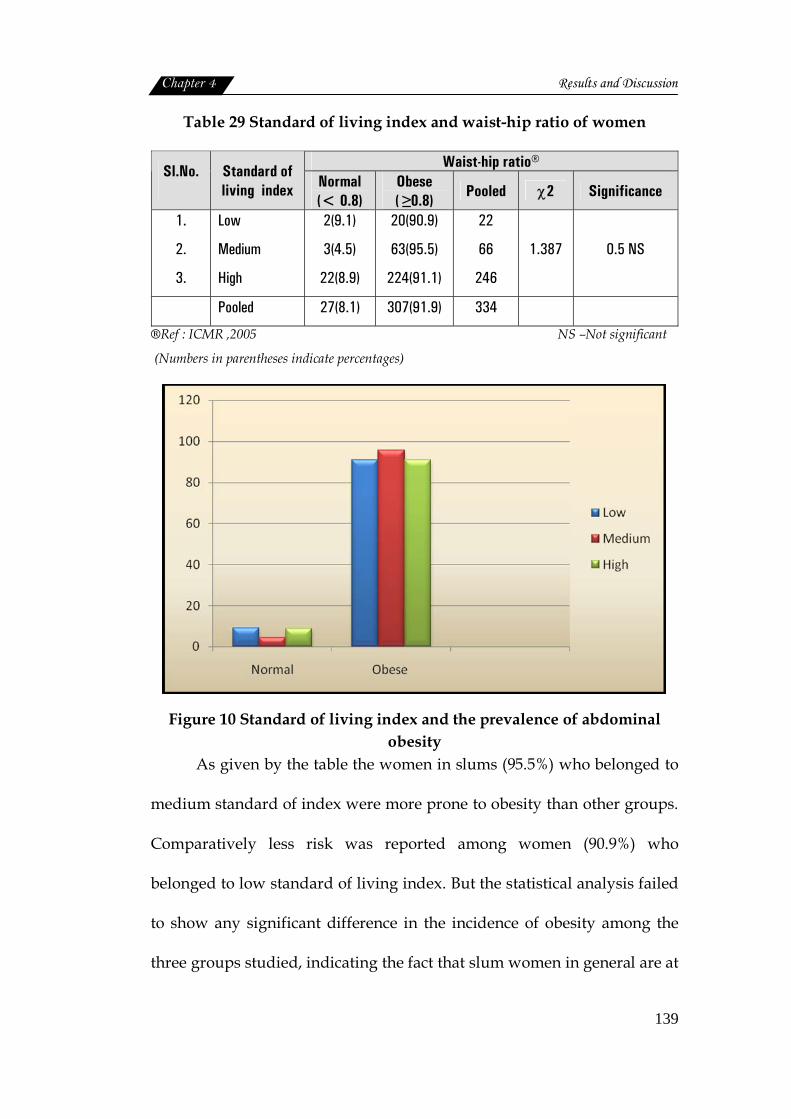
Standard of living index and waist-hip ratio
Based on their standard of living index the waist-hip ratio of the
sample was analysed and the results are presented in the following table.
Chapter 4 Results and Discussion
139
Table 29 Standard of living index and waist-hip ratio of women
Waist-hip ratio® Sl.No.
Standard of living index Normal
(< 0.8) Obese ( ≥0.8)
Pooled χ2 Significance
1.
2.
3.
Low
Medium
High
2(9.1)
3(4.5)
22(8.9)
20(90.9)
63(95.5)
224(91.1)
22
66
246
1.387 0.5 NS
Pooled 27(8.1) 307(91.9) 334
®Ref : ICMR ,2005 NS –Not significant
(Numbers in parentheses indicate percentages)
Figure 10 Standard of living index and the prevalence of abdominal obesity
As given by the table the women in slums (95.5%) who belonged to
medium standard of index were more prone to obesity than other groups.
Comparatively less risk was reported among women (90.9%) who
belonged to low standard of living index. But the statistical analysis failed
to show any significant difference in the incidence of obesity among the
three groups studied, indicating the fact that slum women in general are at

Chapter 4 Results and Discussion
140
the risk of obesity. This finding is illustrated in Figure 10. Waist-hip ratio
as given by Ahmad et al. (2007) is the dominant risk factor predicting
coronary heart disease.
4.2.1.2 Blood haemoglobin status
Blood samples of the entire study population was collected and
analyzed using cyanmethaemoglobin method. The results were compared
with WHO (1968) standards and are presented in table 30.
Table 30 Haemoglobin status of women
Blood haemoglobin®
Sl.No
Age (yrs) Normal
(>12 g/dl)
Mild anaemia
(>10-11.9 g/dl)
Moderate anaemia
(7-10 g/dl) χ2 Significance
1 2 3 4
20-25 26-30 31-35 36-40
16 (17.0) 21 (14.7) 15 (17.9)
Nil
64 (68.1) 106 (74.1) 45 (53.6) 11 (84.6)
14 (14.9) 16 (11.2) 24 (28.6) 2 (15.4)
16.26
0.012*
Pooled 52(15.6) 226(67.7) 56(16.8)
(Numbers in parentheses indicate percentages) *significant at 5% level ®Ref: WHO,1968
Figure 11 Age wise prevalence of anaemia
Chapter 4 Results and Discussion
141
The haemoglobin status arrived at, using the anaemia classification
recommended by WHO (1968) for adult women (non-pregnant and non-
lactating) indicated the prevalence of mild anaemia among majority
(67.7%) of the sample. This was followed by moderate anaemia (16.8%).
Normal haemoglobin status was seen only among 15.6 percent of the
sample.
Age wise classification of haemoglobin status showed that women
in the age group of 36 to 40 years were seriously affected either by mild
(84.6%) or moderate anaemia (15.4%). Nobody found to have normal
haemoiglobin status in this group. This was followed by 26 to 30 year age
group, where mild and moderate anaemia were detected among 74.1
percent and 11.2 percent of women respectively.
Women of 20 to 25 years of age ranked in the rate of anaemia
prevalence. This age wise differences in the incidence of anaemia among
women residing in urban slums, was also found to be statistically
significant at 5 percent level.
Studies by Bentley and Griffiths (2003) stated that prevalence of
anaemia was high among women; 32.4 percent of women had mild
anaemia, 14.19 percent had moderate, and 2.2 percent had severe anaemia.
Slum locations and haemoglobin status
An attempt was made to find out the association between the area
of residence and the prevalence of anaemia among sample. The results are
presented in table 31.
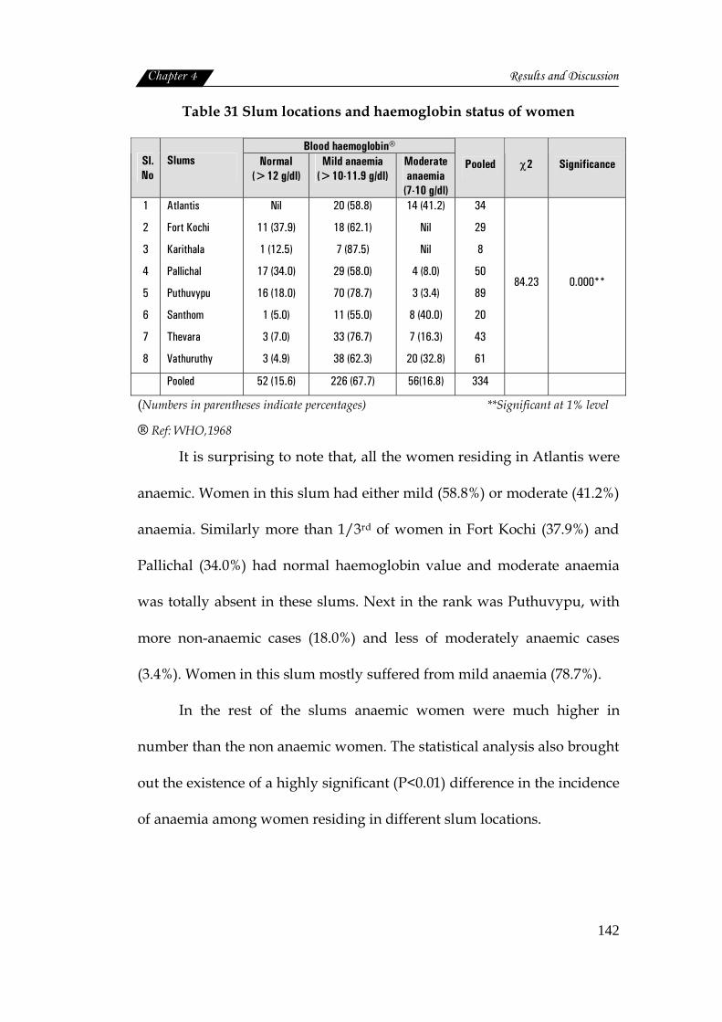
Chapter 4 Results and Discussion
142
Table 31 Slum locations and haemoglobin status of women
Blood haemoglobin® Sl.No
Slums Normal (>12 g/dl)
Mild anaemia (>10-11.9 g/dl)
Moderate anaemia
(7-10 g/dl)
Pooled χ2 Significance
1
2
3
4
5
6
7
8
Atlantis
Fort Kochi
Karithala
Pallichal
Puthuvypu
Santhom
Thevara
Vathuruthy
Nil
11 (37.9)
1 (12.5)
17 (34.0)
16 (18.0)
1 (5.0)
3 (7.0)
3 (4.9)
20 (58.8)
18 (62.1)
7 (87.5)
29 (58.0)
70 (78.7)
11 (55.0)
33 (76.7)
38 (62.3)
14 (41.2)
Nil
Nil
4 (8.0)
3 (3.4)
8 (40.0)
7 (16.3)
20 (32.8)
34
29
8
50
89
20
43
61
84.23 0.000**
Pooled 52 (15.6) 226 (67.7) 56(16.8) 334
(Numbers in parentheses indicate percentages) **Significant at 1% level
® Ref: WHO,1968
It is surprising to note that, all the women residing in Atlantis were
anaemic. Women in this slum had either mild (58.8%) or moderate (41.2%)
anaemia. Similarly more than 1/3rd of women in Fort Kochi (37.9%) and
Pallichal (34.0%) had normal haemoglobin value and moderate anaemia
was totally absent in these slums. Next in the rank was Puthuvypu, with
more non-anaemic cases (18.0%) and less of moderately anaemic cases
(3.4%). Women in this slum mostly suffered from mild anaemia (78.7%).
In the rest of the slums anaemic women were much higher in
number than the non anaemic women. The statistical analysis also brought
out the existence of a highly significant (P<0.01) difference in the incidence
of anaemia among women residing in different slum locations.
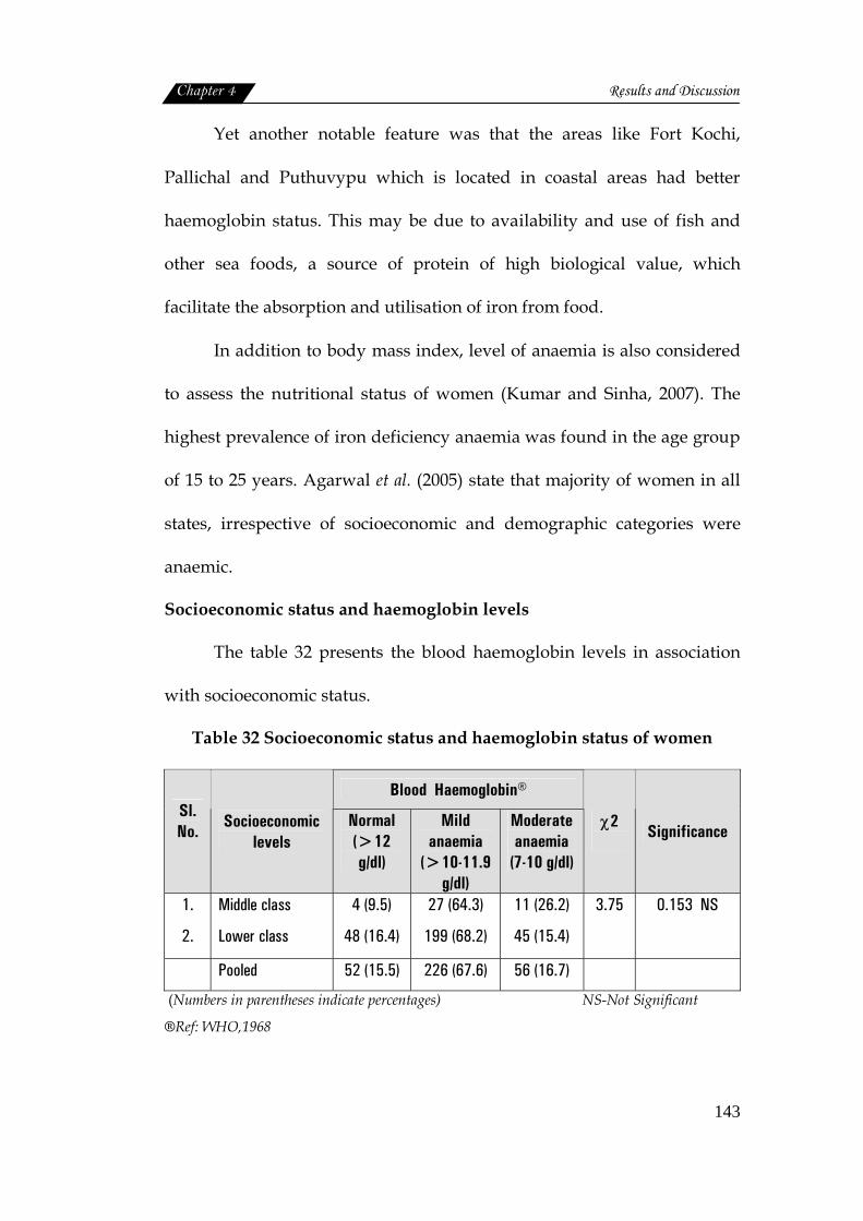
Chapter 4 Results and Discussion
143
Yet another notable feature was that the areas like Fort Kochi,
Pallichal and Puthuvypu which is located in coastal areas had better
haemoglobin status. This may be due to availability and use of fish and
other sea foods, a source of protein of high biological value, which
facilitate the absorption and utilisation of iron from food.
In addition to body mass index, level of anaemia is also considered
to assess the nutritional status of women (Kumar and Sinha, 2007). The
highest prevalence of iron deficiency anaemia was found in the age group
of 15 to 25 years. Agarwal et al. (2005) state that majority of women in all
states, irrespective of socioeconomic and demographic categories were
anaemic.
Socioeconomic status and haemoglobin levels
The table 32 presents the blood haemoglobin levels in association
with socioeconomic status.
Table 32 Socioeconomic status and haemoglobin status of women
Blood Haemoglobin® Sl. No.
Socioeconomic levels
Normal (>12 g/dl)
Mild anaemia
(>10-11.9 g/dl)
Moderate anaemia
(7-10 g/dl)
χ2
Significance
1.
2.
Middle class
Lower class
4 (9.5)
48 (16.4)
27 (64.3)
199 (68.2)
11 (26.2)
45 (15.4)
3.75
0.153 NS
Pooled 52 (15.5) 226 (67.6) 56 (16.7)
(Numbers in parentheses indicate percentages) NS-Not Significant
®Ref: WHO,1968

Chapter 4 Results and Discussion
144
The statistical analysis to know the association between
socioeconomic status and the haemoglobin level showed that no
significant relation existed between these two factors. Infact, as the table
presents, normal cases (non-anaemic women) were more in number in the
lower socioeconomic group (16.4%) than middle class group (9.5%). In
general anaemia was more prevalent among middle class group (9.5%). In
general anaemia was more prevalent among middle class women either as
mild anaemia (64.3%) or moderate anaemia (26.2%) So it is obvious that
better socioeconomic status need not necessarily improve the iron
nutritional status of women.
Poverty and low purchasing power often referred as factors
responsible for low dietary intake (NIPCCD, 2007). But the present study
showed that anaemia prevalence is irrespective of economic status.
Standard of living index and haemoglobin status
The blood haemoglobin levels of the sample of different standard of
living index is shown in table 33.
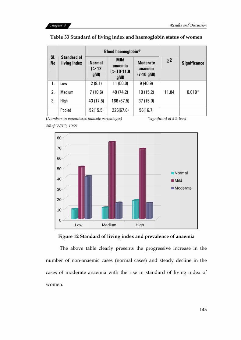
Chapter 4 Results and Discussion
145
Table 33 Standard of living index and haemoglobin status of women
Blood haemoglobin® Sl. No
Standard of living index
Normal (>12 g/dl)
Mild anaemia
(>10-11.9 g/dl)
Moderate anaemia
(7-10 g/dl)
χ2
Significance
1.
2.
3.
Low
Medium
High
2 (9.1)
7 (10.6)
43 (17.5)
11 (50.0)
49 (74.2)
166 (67.5)
9 (40.9)
10 (15.2)
37 (15.0)
11.84
0.019*
Pooled 52(15.5) 226(67.6) 56(16.7)
(Numbers in parentheses indicate percentages) *significant at 5% level
®Ref: WHO, 1968
0
10
20
30
40
50
60
70
80
Low Medium High
Normal
Mild
Moderate
Figure 12 Standard of living index and prevalence of anaemia
The above table clearly presents the progressive increase in the
number of non-anaemic cases (normal cases) and steady decline in the
cases of moderate anaemia with the rise in standard of living index of
women.

Chapter 4 Results and Discussion
146
But prevalence of mild anemia was more among women of medium
(74.2%) and high (67.5%) standard of living index than the low (50.0%)
index group. Statistical analysis also showed a significant association at 5
percent level, between the haemoglobin status and standard of living
index of women at slums.
Mathur and Kachhawaha (2009) found that various factors like
vegetarian diet, low socioeconomic status, low iron intake and history of
excessive menstrual bleeding showed significant association with
anaemia. However age and education did not contribute significantly.
As per the study reports by Verma et al. (2009) clinical signs and
haemoglobin estimation showed that 51 percent were anaemic with the
haemoglobin level ranging from 6.8 to 10.8 g/dl. NFHS-3 (2006) reported
that the anaemia prevalence levels are more than two times higher among
women than men with almost half suffered from moderate to severe
anaemia.
Women in slums of Jammu city suffered from anaemia, they even
showed symptoms like pale conjunctiva, pale nails and pale face. The
women experienced weakness, fatigue and breathlessness due to this
(Kotwal et al., 2008).
4.2.1.3 Dietary assessment
FAO suggested that dietary surveys among individuals provide
information that can be used to describe differences in intake of food and
nutrients. Dietary assessment methods are invaluable tools not only for

Chapter 4 Results and Discussion
147
measuring energy, protein and macronutrient intakes, which serve as the
basis for estimating the prevalence of hunger, but also for assessing
micronutrient deficiencies (ICDAM,2003).
Food habits and practices
All the 334 families included in the study followed non-vegetarian
food habits.
Food selection
The criteria for food selection are influenced by number of
socioeconomic, cultural and spiritual factors. An attempt was made to
study this aspect as it plays decisive role on the food consumption pattern
of individuals and family. Data gathered in this respect was analysed and
the results are given in table 34.
Table 34 Criteria for food selection
Sl. No.
Particulars
Frequency* (n=334)
1.
2.
3.
4.
5.
6.
7.
Ease of Preparation
Freshness
Seasonal food
Local availability
Nutritional Quality
Likes and dislikes of family
Cost
327 (97.9)
320 (95.8)
317 (94.9)
250 (74.9)
182 (54.5)
151 (45.2)
149 (44.6)
(Numbers in parentheses indicate percentages)
*indicates multiple response
As the table depicts, there were seven criteria that women
considered during food selection either by itself or in combination. The
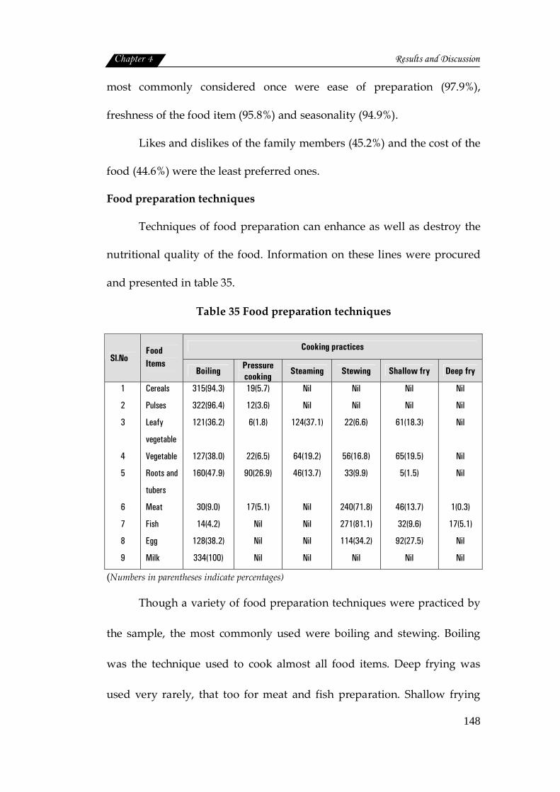
Chapter 4 Results and Discussion
148
most commonly considered once were ease of preparation (97.9%),
freshness of the food item (95.8%) and seasonality (94.9%).
Likes and dislikes of the family members (45.2%) and the cost of the
food (44.6%) were the least preferred ones.
Food preparation techniques
Techniques of food preparation can enhance as well as destroy the
nutritional quality of the food. Information on these lines were procured
and presented in table 35.
Table 35 Food preparation techniques
Cooking practices Sl.No
Food Items
Boiling Pressure cooking Steaming Stewing Shallow fry Deep fry
1
2
3
4
5
6
7
8
9
Cereals
Pulses
Leafy
vegetable
Vegetable
Roots and
tubers
Meat
Fish
Egg
Milk
315(94.3)
322(96.4)
121(36.2)
127(38.0)
160(47.9)
30(9.0)
14(4.2)
128(38.2)
334(100)
19(5.7)
12(3.6)
6(1.8)
22(6.5)
90(26.9)
17(5.1)
Nil
Nil
Nil
Nil
Nil
124(37.1)
64(19.2)
46(13.7)
Nil
Nil
Nil
Nil
Nil
Nil
22(6.6)
56(16.8)
33(9.9)
240(71.8)
271(81.1)
114(34.2)
Nil
Nil
Nil
61(18.3)
65(19.5)
5(1.5)
46(13.7)
32(9.6)
92(27.5)
Nil
Nil
Nil
Nil
Nil
Nil
1(0.3)
17(5.1)
Nil
Nil
(Numbers in parentheses indicate percentages)
Though a variety of food preparation techniques were practiced by
the sample, the most commonly used were boiling and stewing. Boiling
was the technique used to cook almost all food items. Deep frying was
used very rarely, that too for meat and fish preparation. Shallow frying
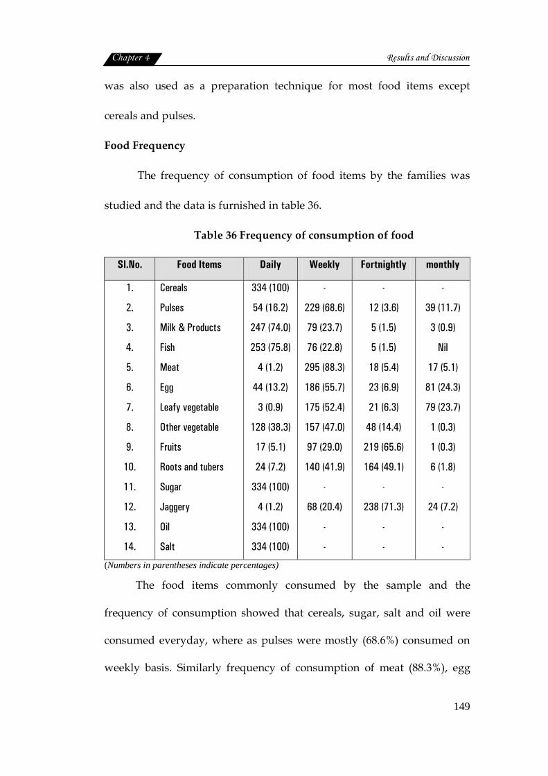
Chapter 4 Results and Discussion
149
was also used as a preparation technique for most food items except
cereals and pulses.
Food Frequency
The frequency of consumption of food items by the families was
studied and the data is furnished in table 36.
Table 36 Frequency of consumption of food
Sl.No. Food Items Daily Weekly Fortnightly monthly
1.
2.
3.
4.
5.
6.
7.
8.
9.
10.
11.
12.
13.
14.
Cereals
Pulses
Milk & Products
Fish
Meat
Egg
Leafy vegetable
Other vegetable
Fruits
Roots and tubers
Sugar
Jaggery
Oil
Salt
334 (100)
54 (16.2)
247 (74.0)
253 (75.8)
4 (1.2)
44 (13.2)
3 (0.9)
128 (38.3)
17 (5.1)
24 (7.2)
334 (100)
4 (1.2)
334 (100)
334 (100)
-
229 (68.6)
79 (23.7)
76 (22.8)
295 (88.3)
186 (55.7)
175 (52.4)
157 (47.0)
97 (29.0)
140 (41.9)
-
68 (20.4)
-
-
-
12 (3.6)
5 (1.5)
5 (1.5)
18 (5.4)
23 (6.9)
21 (6.3)
48 (14.4)
219 (65.6)
164 (49.1)
-
238 (71.3)
-
-
-
39 (11.7)
3 (0.9)
Nil
17 (5.1)
81 (24.3)
79 (23.7)
1 (0.3)
1 (0.3)
6 (1.8)
-
24 (7.2)
-
-
(Numbers in parentheses indicate percentages)
The food items commonly consumed by the sample and the
frequency of consumption showed that cereals, sugar, salt and oil were
consumed everyday, where as pulses were mostly (68.6%) consumed on
weekly basis. Similarly frequency of consumption of meat (88.3%), egg

Chapter 4 Results and Discussion
150
(55.7%), leafy vegetables (52.4%) and vegetables was mostly on weekly
basis. Mostly fruits (65.6%), root and tubers (49.1%) were consumed only
once in a fortnight.
Inadequate representation of fruits and leafy vegetable in the daily
diet was clearly brought out in the present study. Similar findings were
reported by NFHS-3 (2006) stating that 60 percent of women do not
consume fruits even once in a week.
Use of iodised salt
Iodine deficiency has been called the world's major cause of
preventable mental retardation (AIIMS, 2002). On the recommendations of
Central Council of Health in 1984, the Government took policy decision to
iodise the entire edible salt in the country. The details on consumption of
iodised salt is furnished in the following table.
Table 37 Use of Iodised salt by the sample
Sl. No Particulars Frequency* (n=334)
1
2.
Use of iodised salt Regular use Branded packet Powder form Quantity 500 gm and more/month Stored in covered container Stored in the packet itself Kept in kitchen shelf Awareness on iodised salt Iodized is better than non iodised Helps to prevent goitre
208 (62.3) 228 (68.3) 327 (97.9) 327 (97.9) 296 (88.6) 38 (11.4)
211 (63.2)
232 (69.5) 182 (54.5)
(Numbers in parentheses indicate percentages) *indicates multiple response
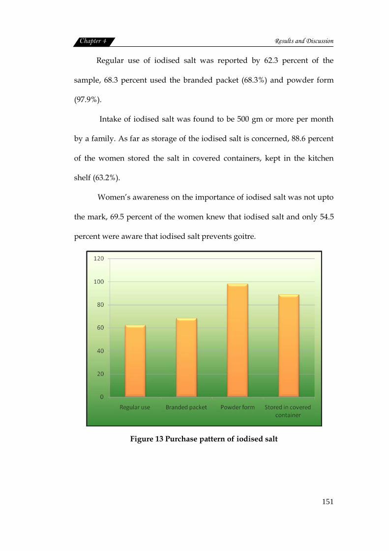
Chapter 4 Results and Discussion
151
Regular use of iodised salt was reported by 62.3 percent of the
sample, 68.3 percent used the branded packet (68.3%) and powder form
(97.9%).
Intake of iodised salt was found to be 500 gm or more per month
by a family. As far as storage of the iodised salt is concerned, 88.6 percent
of the women stored the salt in covered containers, kept in the kitchen
shelf (63.2%).
Women’s awareness on the importance of iodised salt was not upto
the mark, 69.5 percent of the women knew that iodised salt and only 54.5
percent were aware that iodised salt prevents goitre.
Figure 13 Purchase pattern of iodised salt
Chapter 4 Results and Discussion
152
Consumption of inadequately iodised salt combined with the lack
of awareness and improper practices is a major hindrance in the
elimination of IDD’s (Samal et al., 2009).
Prevalence of goitre was high among school children in Belgaum
district (Kamath et al., 2009). A similar study conducted in Trivandrum
district of Kerala, also showed that the overall prevalence of goiter in the
study population was 12.9 percent even though majority (92.8%) of the
subjects claimed to use iodised salt (Libu and Balakrishnan, 2009). As per
NFHS-3(2006) reports only about half of the households in India use
cooking salt which is adequately iodised.
Food consumption pattern of women
Food intake
The recommended dietary allowances are estimates of nutrients to be
consumed daily to ensure the requirements of all individuals in a given
population (ICMR, 2004). The average daily intakes of food was assessed and
compared with RDA (ICMR, 2004). The results are furnished in table 38.
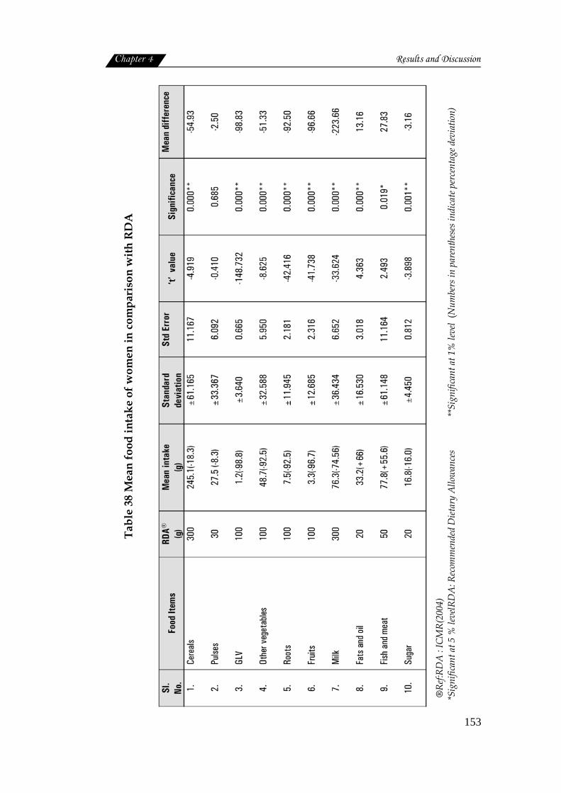
Chapter 4 Results and Discussion
153
Tabl
e 38
Mea
n fo
od in
take
of w
omen
in c
ompa
riso
n w
ith R
DA
®Re
f:RD
A :
ICM
R(20
04)
*Sig
nific
ant a
t 5 %
leve
lRD
A: R
ecom
men
ded
Diet
ary
Allo
wan
ces
**Si
gnifi
cant
at 1
% le
vel
(Num
bers
in p
aren
thes
es in
dica
te p
erce
ntag
e dev
iatio
n)
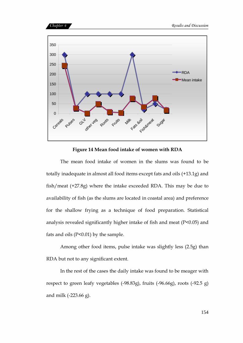
Chapter 4 Results and Discussion
154
0
50
100
150
200
250
300
350
Cereals
Pulses GLV
other
veg
Roots
Fruits Milk
Fats &oil
Fish&mea
tSug
ar
RDA
Mean intake
Figure 14 Mean food intake of women with RDA
The mean food intake of women in the slums was found to be
totally inadequate in almost all food items except fats and oils (+13.1g) and
fish/meat (+27.8g) where the intake exceeded RDA. This may be due to
availability of fish (as the slums are located in coastal area) and preference
for the shallow frying as a technique of food preparation. Statistical
analysis revealed significantly higher intake of fish and meat (P<0.05) and
fats and oils (P<0.01) by the sample.
Among other food items, pulse intake was slightly less (2.5g) than
RDA but not to any significant extent.
In the rest of the cases the daily intake was found to be meager with
respect to green leafy vegetables (-98.83g), fruits (-96.66g), roots (-92.5 g)
and milk (-223.66 g).
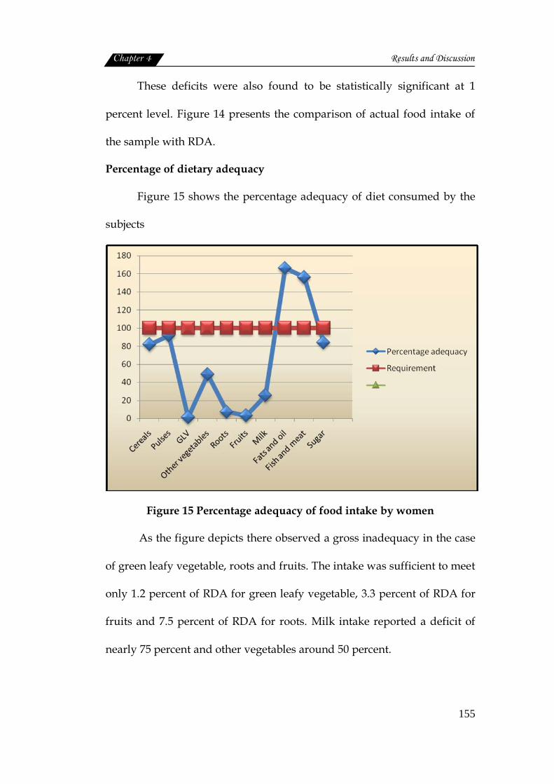
Chapter 4 Results and Discussion
155
These deficits were also found to be statistically significant at 1
percent level. Figure 14 presents the comparison of actual food intake of
the sample with RDA.
Percentage of dietary adequacy
Figure 15 shows the percentage adequacy of diet consumed by the
subjects
Figure 15 Percentage adequacy of food intake by women
As the figure depicts there observed a gross inadequacy in the case
of green leafy vegetable, roots and fruits. The intake was sufficient to meet
only 1.2 percent of RDA for green leafy vegetable, 3.3 percent of RDA for
fruits and 7.5 percent of RDA for roots. Milk intake reported a deficit of
nearly 75 percent and other vegetables around 50 percent.
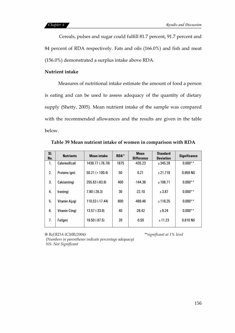
Chapter 4 Results and Discussion
156
Cereals, pulses and sugar could fulfill 81.7 percent, 91.7 percent and
84 percent of RDA respectively. Fats and oils (166.0%) and fish and meat
(156.0%) demonstrated a surplus intake above RDA.
Nutrient intake
Measures of nutritional intake estimate the amount of food a person
is eating and can be used to assess adequacy of the quantity of dietary
supply (Shetty, 2005). Mean nutrient intake of the sample was compared
with the recommended allowances and the results are given in the table
below.
Table 39 Mean nutrient intake of women in comparison with RDA
Sl. No. Nutrients Mean intake RDA® Mean
Difference Standard Deviation Significance
1.
2.
3.
4.
5.
6.
7.
Calories(Kcal)
Proteins (gm)
Calcium(mg)
Iron(mg)
Vitamin A(µg)
Vitamin C(mg)
Fat(gm)
1439.77 (-76.78)
50.21 (+100.4)
255.63 (-63.9)
7.90 (-26.3)
110.53 (-17.44)
13.57 (-33.9)
19.50 (-97.5)
1875
50
400
30
600
40
20
-435.23
0.21
-144.36
-22.10
-489.46
-26.42
-0.50
±345.28
±21.718
±108.71
±3.87
±116.25
±9.24
±11.23
0.000**
0.959 NS
0.000**
0.000**
0.000**
0.000**
0.810 NS
® Ref:RDA-ICMR(2004) **significant at 1% level (Numbers in parentheses indicate percentage adequacy) NS- Not Significant
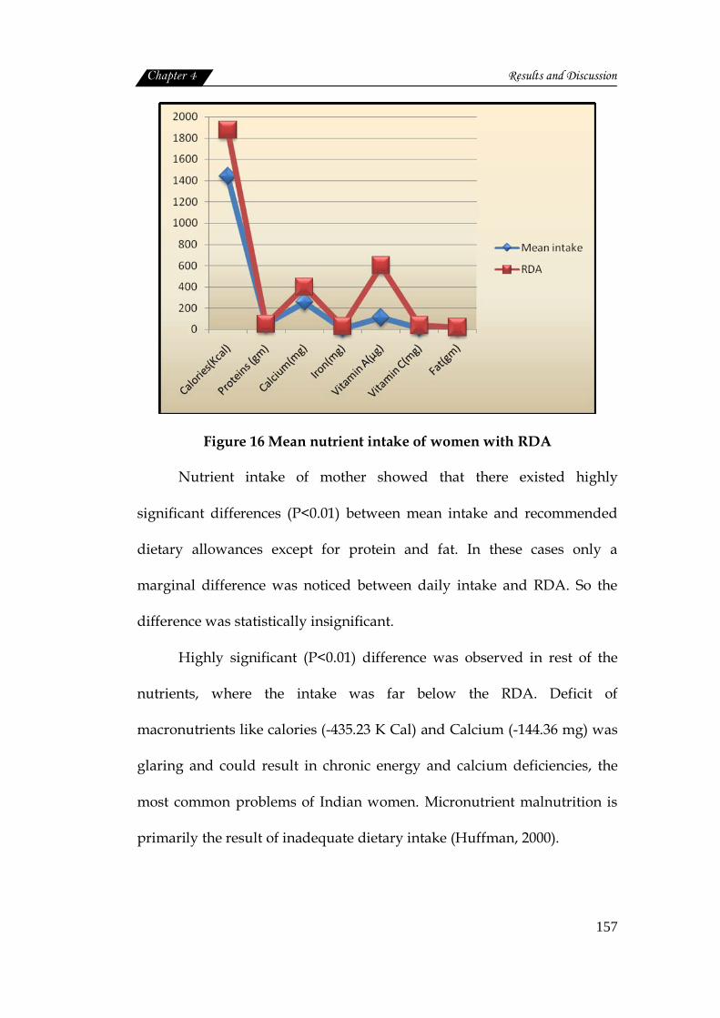
Chapter 4 Results and Discussion
157
Figure 16 Mean nutrient intake of women with RDA
Nutrient intake of mother showed that there existed highly
significant differences (P<0.01) between mean intake and recommended
dietary allowances except for protein and fat. In these cases only a
marginal difference was noticed between daily intake and RDA. So the
difference was statistically insignificant.
Highly significant (P<0.01) difference was observed in rest of the
nutrients, where the intake was far below the RDA. Deficit of
macronutrients like calories (-435.23 K Cal) and Calcium (-144.36 mg) was
glaring and could result in chronic energy and calcium deficiencies, the
most common problems of Indian women. Micronutrient malnutrition is
primarily the result of inadequate dietary intake (Huffman, 2000).
Chapter 4 Results and Discussion
158
In the present study also the micronutrient status of women was
very pathetic. The mean intake of iron was only 7.9 mg/day as against the
RDA of 30 mg/day showing a deficit of 22.1 mg. Similarly vitamin A
intake was 110.53 µg and RDA was 600 µg/ day. The deficit was 489.46 µg.
Low dietary intake and poor iron and folic acid intake are major
factors responsible for high prevalence of anaemia in India (Shetty, 2005).
The micronutrient status of women in developing countries according to
Huffman (2000) affects their health during pregnancy and lactation, the
outcomes of their pregnancies, and the health of their infants. The high
rate of prevalence of anaemia among the study population, reported in the
previous section of this report may mainly be due to this dietary
inadequacy of iron. Figure 16 illustrates the comparison of actual nutrient
intake of women with RDA
Calcium intake was less with mean intake of 255.63 mg, when
compared with RDA of 400 mg. The status of iron showed that intake was
significantly low, with mean intake of 7.9mg corresponding to a
requirement of 30mg. Vitamin C deficiency was also significant with mean
intake less than RDA. Fat intake was slightly less than the requirement,
while protein intake was slightly more than the requirement.
Percentage of nutritional adequacy
The details are given in figure 17.
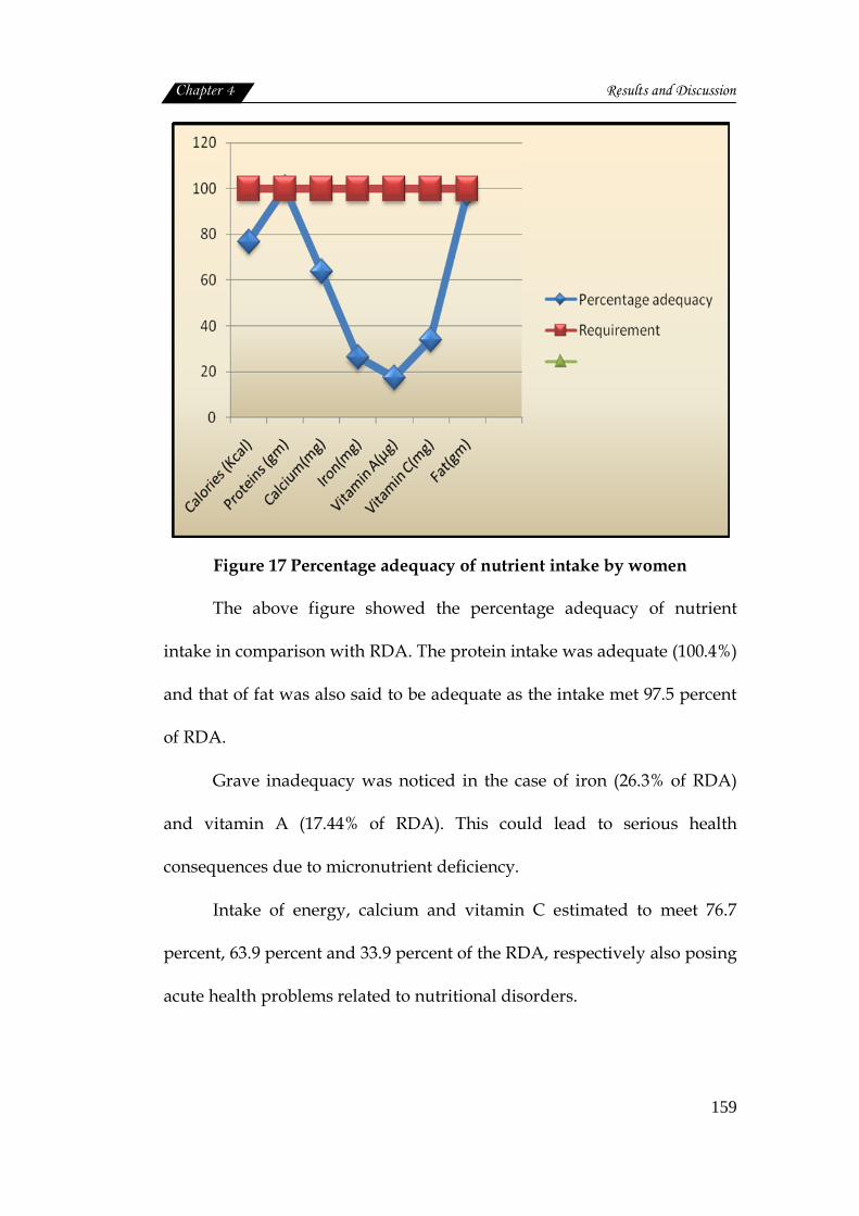
Chapter 4 Results and Discussion
159
Figure 17 Percentage adequacy of nutrient intake by women
The above figure showed the percentage adequacy of nutrient
intake in comparison with RDA. The protein intake was adequate (100.4%)
and that of fat was also said to be adequate as the intake met 97.5 percent
of RDA.
Grave inadequacy was noticed in the case of iron (26.3% of RDA)
and vitamin A (17.44% of RDA). This could lead to serious health
consequences due to micronutrient deficiency.
Intake of energy, calcium and vitamin C estimated to meet 76.7
percent, 63.9 percent and 33.9 percent of the RDA, respectively also posing
acute health problems related to nutritional disorders.
Chapter 4 Results and Discussion
160
Thus it can be stated that diet consumed by the women of urban slums,
under the study, is totally inadequate in quantity as well as quality. As
NFHS-3 (2006) reported rather than quantity the diet of the women should
made nutrient dense especially micronutrients.
4.2.2 Health status of women
Women’s health during the reproductive or fertile years is relevant
not only for themselves, but also has an impact on the health and develop-
ment of the next generation (WHO, 2009). This section deals with the
various health problems, the women encountered during the prime period
of life.
4.2.2.1 Incidence of health problems
The health problems were categorised as metabolic related,
nutritional deficiencies, reproductive health and other minor ailments. The
information gathered in this respect were analysed and the findings are
summarised below:
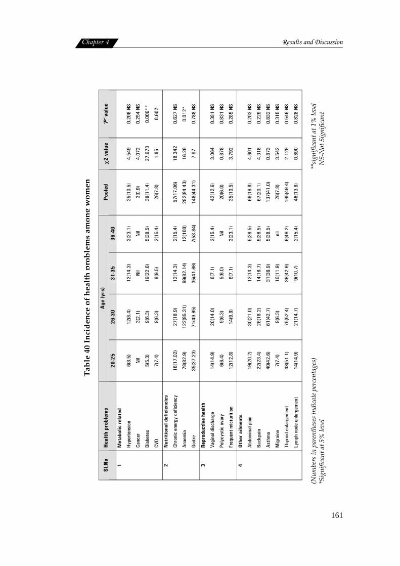
Chapter 4 Results and Discussion
161
Table 40 Incidence of health problems among women
(Num
bers
in p
aren
thes
es in
dica
te p
erce
ntag
es)
**s
igni
fican
t at 1
% le
vel
*Sig
nific
ant a
t 5%
leve
l
NS-
Not
Sig
nific
ant
Chapter 4 Results and Discussion
162
Metabolic related problems
The metabolic disorders like hypertension (10.5%), diabetes (11.4%),
CVD (7.8%) and Cancer (0.9%) were diagnosed through medical screening
of women, residing in slums. All these were found to occur even at the
younger age of 20 to 25 years among women residing in slums. The rate of
incidence was highest in the case of hypertension (8.5%) and lowest for
diabetes (5.3%) and CVD (7.4%) ranked in between. As the age advances
incident rate was also progressively increased and at middle age there
observed the highest prevalence of diabetes (38.5%), hypertension (23.1%)
and CVD (15.4%). High blood pressure is the leading risk for adult women
everywhere and is responsible for 18 percent of deaths of women over 20
years of age. High blood pressure, high blood glucose levels, physical
inactivity and high serum cholesterol cause similar proportions of deaths
across all income levels (WHO, 2010).
Incidence of cancer (breast cancer) was reported among 2.1 percent
of women. Statistical analysis proved to have a highly significant
association (P<0.01) between age and prevalence of diabetes among
women. But the rest of the diseases failed to show any significant
association with age. However it is worth noticed that diabetes and
hypertension were on increase among women at productive age (20 to 40
Chapter 4 Results and Discussion
163
years) which may soon develop as cardio vascular problems leading to
disability and low productivity.
In 2004, cancers killed just fewer than one million women aged 20 to
59 years, with 80 percent of these deaths occurring in low and middle-
income countries, where women consistently have a lower cancer survival
rate because of limited access to screening, late diagnosis and inadequate
access to effective treatment (Kamangar et al., 2005; Parkin et al., 2002).
Nutritional deficiencies
Another observation through clinical screening of the sample was
incidence nutritional deficiency diseases, such as anaemia (82.9%), goitre
(37.23%) and chronic energy deficiency (17.02%) at the age of 20 to 25
years.
Prevalence of anaemia and goitre, both tend to increase with age.
Whereas chronic energy deficiency failed to show such a trend. One
hundred percent anaemia was reported in the age group of 36 to 40 years,
with an overall prevalence of 84.43 percent disturbed menstrual cycle
excessive bleeding and low intake of iron all may contribute to the above
situation. Role of goitre and related hormonal imbalance also, cannot be
overlooked in this respect.
Goitre prevalence at the age 36 to 40 years, was 53.84 percent with
an overall prevalence of 44.31 percent. This situation also warrants
Chapter 4 Results and Discussion
164
immediate attention. The association of age with incidence of nutritional
deficiencies, when studied a statistical significance at 5 percent level was
obtained only in the case of iron deficiency anaemia.
Reproductive health
Vaginal discharge, a symptom of reproductive tract infection was
detected among 12.6 percent of women at slums. The problem was more
among the age group of 36 to 40 years (15.4%), and 20 to 25 years (14.9%).
Irrespective of the age around 6.0 percent of the sample had polycystic
ovary syndrome. The problem of frequent micturition was also reported
by 10.5 percent of the sample, with highest incidence among 36 to 40 years
(23.1%).
The significant differences in reproductive health outcomes exist
among women from slum and non-slum. The use of skilled delivery care
was found to be significantly associated with age, level of education,
economic status, parity, and prior antenatal visits (Hazarika, 2010). The
health of women is also linked to their status in the society (Rao et al.,
2010).
Other ailments
Other ailments like thyroid enlargement (49.4%), asthma (41.0%),
back pain (20.1%) and abdominal pain (19.8%) were also noticed among
the sample. Thyroid enlargement was more among women of 26 to 30
Chapter 4 Results and Discussion
165
years (52.4%), all the other age groups also had a relatively high incidence
of this problem.
Asthma was yet another problem commonly found among women.
Relatively high incidence was reported by all age groups. Insanitary living
environment may be a reason for this episode.
Back pain was more among the older age group of 36 to 40 years
(38.5%), and about 23.4 percent in the age group of 20 to 25 years of age.
Asthma, heart disease, arthritis, depression and diabetes are
common in women and they are seen particularly in poorer women and
those living in rural areas (World Health Survey, 2009). Migraine
problems were more among 31 to 35 years of age (11.9%), and least among
25 to 30 years of age (6.3%). Among the entire sample 7.8 percent had
migraine.
Slum locations and health problems
Slum wise prevalence of various health problems was statistically
analysed. The results are shown in table 41.
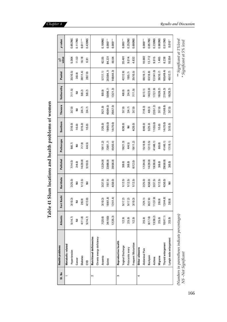
Chapter 4 Results and Discussion
166
Table 41 Slum locations and health problems of women
(Num
bers
in p
aren
thes
es in
dica
te p
erce
ntag
es)
**
Sig
nific
ant a
t 1%
level
N
S –N
ot S
igni
fican
t
* S
igni
fican
t at 5
% le
vel

Chapter 4 Results and Discussion
167
The prevalence of health problems of women was studied under
four heads, and it was found that the overall prevalence rate was highest
for nutritional deficiencies (17.1% to 84.7 %), followed by other ailments
(10.7% to 49.4%). Reproductive health related problems (5.7% to 12.6%)
and metabolic disorders (0.92% to 11.4%) contributed a comparatively
minor share to the disease profile.
The slum wise distribution of health problems brought out very
clearly the distressing state of Santhom slum, with highest prevalence of
maximum number of episodes of illness. Next in the list was Karithala and
Pallichal. Women in both the slums were equally exposed to serious
health problems.
A comparatively better profile was presented by Atlantis and
Thevara slums having slightly less number of acute cases. But incidence of
anaemia, goitre and asthma was invariably high in all slums including
Atlantis and Thevara.
Statistical analysis further revealed that the difference observed in
the incidence of metabolic disorders like hypertension, cancer, diabetes
and CVD among women residing in different slums, were not to any
significant extend, except the incidence of diabetes. In the case of diabetes,
Chapter 4 Results and Discussion
168
the difference was found to be statistically significant at one percent level
(P<0.01).
For nutritional deficiencies also a statistically significant difference
(P<0.01), in the incidence of anaemia and goitre among slums was
reported, showing the strong influence of slum locations on the nutritional
status of women.
As far as the reproductive health problems are concerned, women
having the problems of vaginal discharge showed a statistically significant
difference (P<0.01) with slums
Similarly among other ailments, like abdominal pain and
lymphnode enlargement were the two health problems showed
statistically significant difference in their occurrence in slums.
Socioeconomic status and health problems

Chapter 4 Results and Discussion
169
Table 42 Socioeconomic status and health problems of women
Sl. No Health problems Middle
Class Low Class Pooled χ2value P value
1
Metabolic related
Hypertension
Cancer
Diabetes
Cardio vascular disease
6(14.3)
2(4.8)
5(11.9)
6(14.3)
29(9.9)
1(0.3)
33(11.3)
20(6.8)
35(10.5)
3(0.9)
38(11.4)
26(7.8)
0.742
8.025
0.013
2.829
0.389 NS
0.005**
0.908NS
0.093 NS
2
Nutritional deficiencies
Chronic energy deficiency
Anaemia
Goitre
4(9.5)
38(90.5)
21(50.0)
53(18.2)
244(83.6)
127(43.5)
57(17.1)
282(84.4)
148(44.3)
4.22
3.75
1.75
0.754NS
0.153NS
0.782NS
3
Reproductive health
Vaginal Discharge
Polycystic ovary
Frequent micturition
6(14.3)
4(9.5)
4(9.5)
36(12.3)
16(5.5)
33(11.3)
42(12.6)
20(6.0)
35(10.5)
0.128
1.067
1.674
0.721 NS
0.302 NS
0.196 NS
4
Other ailments
Abdominal Pain
Back pain
Asthma
Migraine
Thyroid enlargement
Lymph node enlargement
5(11.9)
7(16.7)
23(54.8)
nil
23(54.8)
4(9.5)
61(20.9)
60(20.5)
114(39.0)
26(8.9)
142(48.6)
42(14.4)
66(19.8)
67(20.1)
137(41.0)
26(7.8)
165(49.4)
46(13.8)
1.870
0.345
3.751
4.055
0.552
0.730
0.171 NS
0.557 NS
0.053*
0.044*
0.457 NS
0.393 NS
(Numbers in parentheses indicate percentages) **Significant at 1% level NS‐Not Significant *Significant at 5% level
The health problems of women in slums were categorized on the
basis of socioeconomic status computed based on Kuppuswamy scale
(1981). The results are given in table 42.

Chapter 4 Results and Discussion
170
Metabolic related problems
As the table depicts metabolic related disease found to reduce with
the lowering of socioeconomic status. These diseases are often referred as
the diseases of the elite group and product of sedentary life style,
changing food habits and stressful environment. The double burden of
malnutrition and life style diseases among Indian poor has been reported
by several authors.
The present situation is a replica of the above report. Inactivity, low
fibre diet and most importantly the stress situation for slum dwellers may
be the contributory factors for the incidence of metabolic diseases even
among the low income group. This may be slow beginning of an alarming
situation in the future.
The statistical analysis could not show any significance between
middle and low class status in the incidence of metabolic disorders except
cancer. There the difference was highly significant (P<0.01) statistically.
Gopalan (1998) and Popkin et al. (2001) also reported that diabetes,
hypertension, asthma, cardiovascular disease, some cancers, gall bladder
disease and osteoarthritis – all of which are on the rise in developing
countries, particularly among the middle-class, urban populations.
Nutritional deficiencies
As shown in the table, there observed a marginal decline in anaemia
and goitre with lowering of socioeconomic status. Incidence of anaemia
was found to be slightly more among middle (90.5%) than low class

Chapter 4 Results and Discussion
171
(83.6%). Goitre was also more among middle class (50.0%) and less (43.5%)
in low class. At the same time higher prevalence of energy deficiency
(18.2%) was reported among middle class group than their low income
counterparts (9.5%). However the difference observed in the incidence of
nutritional deficiencies due to socioeconomic status were not significant
statistically.
Reproductive health
A reduction in the reproductive health problems like vaginal
discharge and polycystic ovary was reported with the lowering of social
status of women in slum and a reverse trend was seen in the case of
frequent micturition. But statistical analysis proved that there existed no
significant difference in the occurrence of health problems and social
status of women.
Other ailments
Abdominal pain, back pain, migraine and lymphnode enlargement
were found increasing with lowering of social status. Whereas thyroid
enlargement and asthmatic cases were declined as the social status shifted
from middle to lower level. However these difference in the prevalence
were statistically significant at 5 percent level only in the case of asthma
and migraine and insignificant in the rest of the ailments.
Standard of living index and health problems
The details are given in table 43.

Chapter 4 Results and Discussion
172
Table 43 Standard of living index and health problems of women
Sl.no Health problems Low Medium High Pooled χ2 value
P value
1
Metabolic related
Hypertension
Cancer
Diabetes
CVD
4(18.2)
Nil
3(13.6)
1(4.5)
7(10.6)
2(3.0)
5(7.6)
5(7.6)
24(9.8)
1(0.4)
30(12.2)
20(8.1)
35(10.5)
3(0.9)
38(11.4)
26(7.8)
1.530
4.216
1.221
0.366
0.465NS
0.121NS
0.543NS
0.833NS
2
Nutritional deficiencies
Chronic energy
deficiency
Anaemia
Goitre
5(22.7)
20(91.0)
6(27.3)
13(19.7)
59(89.4)
28(42.4)
39(15.9)
203(82.5)
114(46.3)
57(17.06)
282(84.4)
148(44.3)
11.28
11.84
10.57
0.664NS
0.019*
0.227NS
3
Reproductive health
Vaginal Discharge
Polycystic ovary
Frequent micturition
5(22.7)
1(4.5)
4(18.2)
10(15.2)
2(3.0)
8(12.1)
27(11.0)
17(6.9)
23(9.3)
42(12.6)
20(6.0)
35(10.5)
3.034
1.479
1.916
0.219NS
0.477NS
0.384NS
4
Other ailments
Abdominal Pain
Backpain
Asthma
Migraine
Thyroid enlargement
Lymph node enlargement
7(31.8)
5(22.7)
5(22.7)
2(9.1)
7(31.8)
4(18.2)
10(15.2)
11(16.7)
30(45.5)
2(3.0)
38(57.6)
10(15.2)
49(19.9)
51(20.7)
102(41.5)
22(8.9)
120(48.8)
32(13.0)
66(19.8)
67(20.1)
137(41.0)
26(7.8)
165(49.4)
46(13.8)
2.905
0.641
3.599
2.590
4.523
0.587
0.234NS
0.726NS
0.165NS
0.274NS
0.104NS
0.746NS
(Numbers in parentheses indicate percentages) Significant at 5% level NS-Not Significant
Metabolic related diseases
Regarding metabolic disorders a declining trend in hypertension
and an increasing trend in CVD were reported with improvement in
standard of living index. These trend were also found to be insignificant
statistically. Hypertension was found to be more (18.2%) among women of
low standard of living index than middle (10.6%) and high (9.8%).
Chapter 4 Results and Discussion
173
Diabetes was prevalent more among low (13.6%) as well as high
(12.2%) standard living than medium standard of living (7.6%). The
incidence of CVD was highest among women of high standard of living,
followed by medium (8.1%) and low standard of living index (4.5%).
Nutritional Deficiencies
As the table presents the standard of living index did not have any
significant influence on the health profile of women in the slum areas
except for anaemia only here, the standard of living index found to have a
positive influence which was statistically significant at 5 percent level.
Such as improvement in standard of living correspondingly reduced the
incidence of anaemia among women. Among other nutritional deficiencies
chronic energy deficiency also followed the same trend but not to any
significant extent. But goitre presented a reverse trend which was also
significant statistically.
Reproductive health problem
Similarly reproductive health problems were also noticed to reduce
with betterment in standard of living index, but to any significant extent.
Problems related to reproductive health generally tended to reduce with
improvement in standard of living index. But statistically, these changes in
the occurrence of reproductive health problems proved to be insignificant.
Other ailments
With regard to other health problems there was no uniform trend
noticed in their occurrence though changes were noticed in their
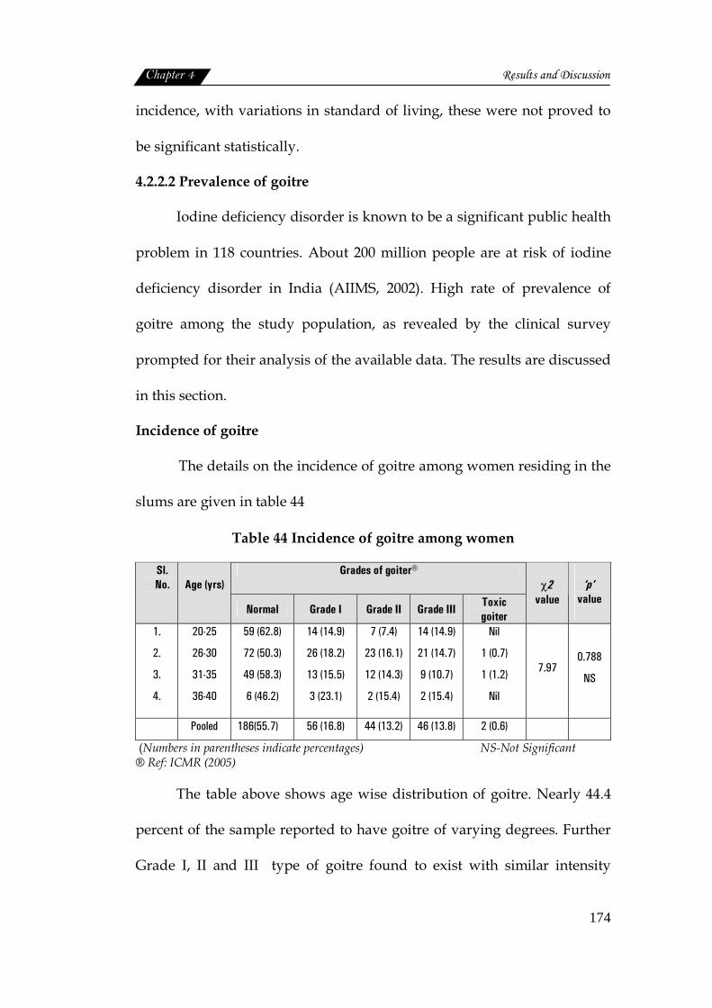
Chapter 4 Results and Discussion
174
incidence, with variations in standard of living, these were not proved to
be significant statistically.
4.2.2.2 Prevalence of goitre
Iodine deficiency disorder is known to be a significant public health
problem in 118 countries. About 200 million people are at risk of iodine
deficiency disorder in India (AIIMS, 2002). High rate of prevalence of
goitre among the study population, as revealed by the clinical survey
prompted for their analysis of the available data. The results are discussed
in this section.
Incidence of goitre
The details on the incidence of goitre among women residing in the
slums are given in table 44
Table 44 Incidence of goitre among women
Grades of goiter® Sl. No.
Age (yrs)
Normal Grade I Grade II Grade III Toxic goiter
χ2
value
‘p’
value
1.
2.
3.
4.
20-25
26-30
31-35
36-40
59 (62.8)
72 (50.3)
49 (58.3)
6 (46.2)
14 (14.9)
26 (18.2)
13 (15.5)
3 (23.1)
7 (7.4)
23 (16.1)
12 (14.3)
2 (15.4)
14 (14.9)
21 (14.7)
9 (10.7)
2 (15.4)
Nil
1 (0.7)
1 (1.2)
Nil
7.97 0.788
NS
Pooled 186(55.7) 56 (16.8) 44 (13.2) 46 (13.8) 2 (0.6)
(Numbers in parentheses indicate percentages) NS-Not Significant ® Ref: ICMR (2005)
The table above shows age wise distribution of goitre. Nearly 44.4
percent of the sample reported to have goitre of varying degrees. Further
Grade I, II and III type of goitre found to exist with similar intensity

Chapter 4 Results and Discussion
175
among women of all age groups, 37.2 percent of women of 20 to 25 years ,
49.7 percent from 26 to 30 years 41.7 percent from 31 to 35 years and 53.9
percent of above 36 years group were reported to be affected. When the
age factor was considered with different grades of goitre, it was seen that
Grade I goitre was more prevalent (23.1%) among women of 36 to 40
years. Irrespective of age Grade II and III goitre was seen among all age
groups.
So statistical analysis failed to show any significant association
between age of women and prevalence of goitre. However seriousness of
the problem cannot be overlooked, because of its wider coverage and
greater intensity; inspite of living in coastal areas.
Studies by Jain et al. (2009) also revealed that severe and moderate
iodine deficiency disorder was reported among 6 percent of children.
Living on the sea coast does not guarantee iodine sufficiency and
significant pockets of iodine deficiency have been reported from the
Goa, Mumbai, Kerala and Andaman and Nicobar Islands. Even those
areas which are presently relatively free of this problem can become
endemic because of intensive agricultural operations and subsequent
depletion of soil (AIIMS, 2002).
Slum locations and incidence of goitre
Iodine deficiency has been called the world's major cause of
preventable mental retardation. Slum wise distribution of sample with
varying degrees of goitre is given in table 45.
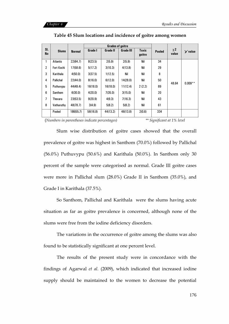
Chapter 4 Results and Discussion
176
Table 45 Slum locations and incidence of goitre among women
Grades of goitre Sl.No
Slums Normal Grade I Grade II Grade III Toxic goitre
Pooled χ2 value
‘p’ value
1
2
3
4
5
6
7
8
Atlantis
Fort Kochi
Karithala
Pallichal
Puthuvypu
Santhom
Thevara
Vathuruthy
22(64.7)
17(58.6)
4(50.0)
22(44.0)
44(49.4)
6(30.0)
23(53.5)
48(78.7)
8(23.5)
5(17.2)
3(37.5)
8(16.0)
16(18.0)
4(20.0)
9(20.9)
3(4.9)
2(5.9)
3(10.3)
1(12.5)
6(12.0)
16(18.0)
7(35.0)
4(9.3)
5(8.2)
2(5.9)
4(13.8)
Nil
14(28.0)
11(12.4)
3(15.0)
7(16.3)
5(8.2)
Nil
Nil
Nil
Nil
2 (2.2)
Nil
Nil
Nil
34
29
8
50
89
20
43
61
48.64 0.009**
Pooled 186(55.7) 56(16.8) 44(13.2) 46(13.8) 2(0.6) 334
(Numbers in parentheses indicate percentages) ** Significant at 1% level
Slum wise distribution of goitre cases showed that the overall
prevalence of goitre was highest in Santhom (70.0%) followed by Pallichal
(56.0%) Puthuvypu (50.6%) and Karithala (50.0%). In Santhom only 30
percent of the sample were categorised as normal. Grade III goitre cases
were more in Pallichal slum (28.0%) Grade II in Santhom (35.0%), and
Grade I in Karithala (37.5%).
So Santhom, Pallichal and Karithala were the slums having acute
situation as far as goitre prevalence is concerned, although none of the
slums were free from the iodine deficiency disorders.
The variations in the occurrence of goitre among the slums was also
found to be statistically significant at one percent level.
The results of the present study were in concordance with the
findings of Agarwal et al. (2009), which indicated that increased iodine
supply should be maintained to the women to decrease the potential
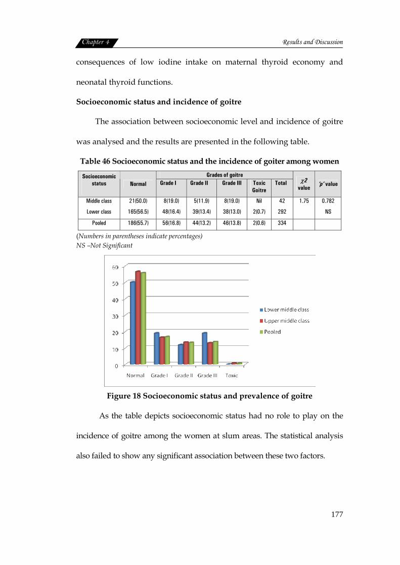
Chapter 4 Results and Discussion
177
consequences of low iodine intake on maternal thyroid economy and
neonatal thyroid functions.
Socioeconomic status and incidence of goitre
The association between socioeconomic level and incidence of goitre
was analysed and the results are presented in the following table.
Table 46 Socioeconomic status and the incidence of goiter among women Grades of goitre Socioeconomic
status Normal Grade I Grade II Grade III Toxic Goitre
Total χ2 value
‘p’ value
Middle class
Lower class
21(50.0)
165(56.5)
8(19.0)
48(16.4)
5(11.9)
39(13.4)
8(19.0)
38(13.0)
Nil
2(0.7)
42
292
1.75
0.782
NS
Pooled 186(55.7) 56(16.8) 44(13.2) 46(13.8) 2(0.6) 334
(Numbers in parentheses indicate percentages) NS –Not Significant
Figure 18 Socioeconomic status and prevalence of goitre
As the table depicts socioeconomic status had no role to play on the
incidence of goitre among the women at slum areas. The statistical analysis
also failed to show any significant association between these two factors.
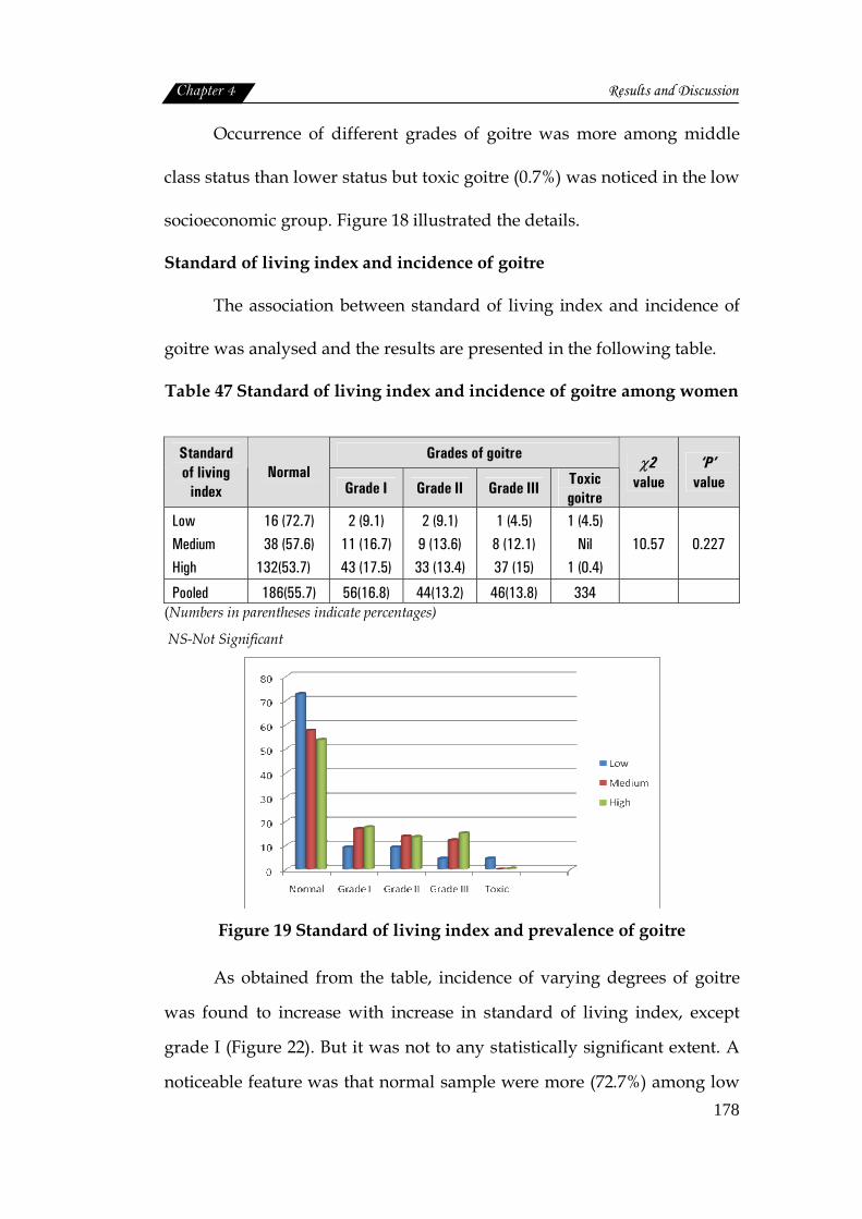
Chapter 4 Results and Discussion
178
Occurrence of different grades of goitre was more among middle
class status than lower status but toxic goitre (0.7%) was noticed in the low
socioeconomic group. Figure 18 illustrated the details.
Standard of living index and incidence of goitre
The association between standard of living index and incidence of
goitre was analysed and the results are presented in the following table.
Table 47 Standard of living index and incidence of goitre among women
Grades of goitre Standard of living
index Normal
Grade I Grade II Grade III Toxic goitre
χ2 value
‘P’ value
Low Medium High
16 (72.7) 38 (57.6)
132(53.7)
2 (9.1) 11 (16.7) 43 (17.5)
2 (9.1) 9 (13.6) 33 (13.4)
1 (4.5) 8 (12.1) 37 (15)
1 (4.5) Nil
1 (0.4)
10.57
0.227
Pooled 186(55.7) 56(16.8) 44(13.2) 46(13.8) 334 (Numbers in parentheses indicate percentages)
NS-Not Significant
Figure 19 Standard of living index and prevalence of goitre
As obtained from the table, incidence of varying degrees of goitre
was found to increase with increase in standard of living index, except
grade I (Figure 22). But it was not to any statistically significant extent. A
noticeable feature was that normal sample were more (72.7%) among low
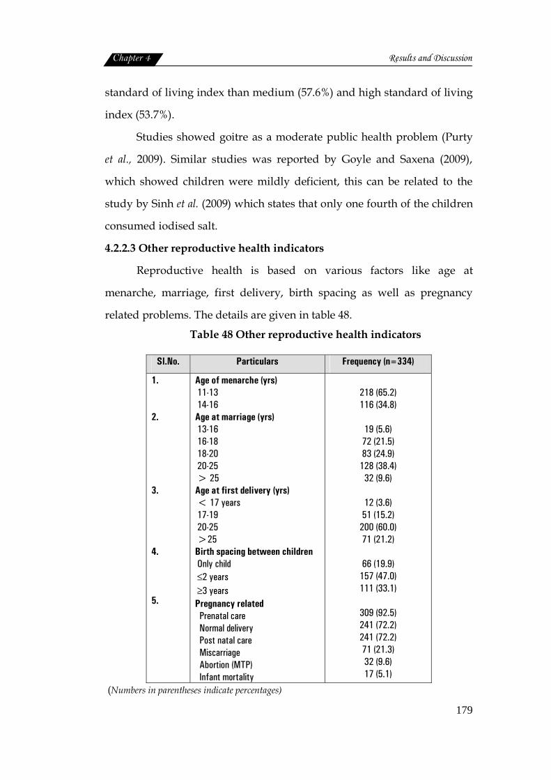
Chapter 4 Results and Discussion
179
standard of living index than medium (57.6%) and high standard of living
index (53.7%).
Studies showed goitre as a moderate public health problem (Purty
et al., 2009). Similar studies was reported by Goyle and Saxena (2009),
which showed children were mildly deficient, this can be related to the
study by Sinh et al. (2009) which states that only one fourth of the children
consumed iodised salt.
4.2.2.3 Other reproductive health indicators
Reproductive health is based on various factors like age at
menarche, marriage, first delivery, birth spacing as well as pregnancy
related problems. The details are given in table 48.
Table 48 Other reproductive health indicators
Sl.No. Particulars Frequency (n=334)
1. 2. 3. 4. 5.
Age of menarche (yrs) 11-13 14-16 Age at marriage (yrs) 13-16 16-18 18-20 20-25 > 25 Age at first delivery (yrs) < 17 years 17-19 20-25 >25 Birth spacing between children Only child ≤2 years ≥3 years Pregnancy related Prenatal care Normal delivery Post natal care Miscarriage Abortion (MTP) Infant mortality
218 (65.2) 116 (34.8)
19 (5.6) 72 (21.5) 83 (24.9)
128 (38.4) 32 (9.6)
12 (3.6) 51 (15.2)
200 (60.0) 71 (21.2)
66 (19.9)
157 (47.0) 111 (33.1)
309 (92.5) 241 (72.2) 241 (72.2) 71 (21.3) 32 (9.6) 17 (5.1)
(Numbers in parentheses indicate percentages)

Chapter 4 Results and Discussion
180
The details of reproductive health showed that the age for menarche
was mostly between 11 to 13 years (65.2%). The age at marriage was
between 20 to 25 years in majority of cases (38.4%), but the age was as low
as 13 to 16 years among 5.6 percent of the sample.
The age at first delivery was found to be 20 to 25 years (60.0%), but
it was less than seventeen years for 3.6 percent and 17 to 19 years for 15.2
percent. Birth spacing was mostly (47.0%) less than 2 years. Prenatal care
(92.5%) and post natal care (72.2%) were taken by the sample, but it can be
observed that post natal care was not given much importance as that of
prenatal care. According to USAID (2010) reported pregnancies in women
under twenty years of age are associated with significant perinatal risks
and that pregnancies in women under sixteen are associated with
significant maternal as well as perinatal risks. NFHS-3 (2006) reported that
in Kerala, 93.9 percent of women had at least three antenatal care for their
last birth.
Miscarriages were more (21.3%) than abortions (9.6%). Cases of
infant mortality were also present (5.1%). Reduction in perinatal mortality
rate may be possible with focussed medical services to women of low
socioeconomic status having bad obstetrical history and those delivering
before term (Kapoor et al., 1996).
The infant mortality rate over this period was 37.9 per 1000 live
births. Over half (54.3%) of the deaths occurred in the neonatal period
(Vaid and Vaid, 2005).
Chapter 4 Results and Discussion
181
4.3 Nutritional and health status of preschool children
Preschool children, a nutritionally vulnerable segment of
population, are also very much susceptible to morbidity due to infections.
Undernutrition among preschool children is one of the greatest public
health problems in developing countries. Undernutrition is the factor
closely associated with child mortality rates (WHO, 1983). The following
sections deal with the various components of nutritional status of
preschool children.
4.3.1 Nutritional status of preschoolers
Nutrition is an input to and foundation for health and development
(WHO, 2010). Childhood undernutrition remains a major health problem
in India especially in slums (Bisai et al., 2009). To assess the nutritional
status of children a number of techniques are made use of in these days.
4.3.1.1 Nutritional anthropometry
Child growth is the most widely used indicator of nutritional status
(World Health Statistics, 2009). Anthropometric measurements are the
most widely used method to assess nutritional status. The use of these
measurements depends on age assessment and normal values for
comparison (ICMR, 2005).
Age and gender wise distribution
Age and gender wise distribution of the sample is presented in
table.

Chapter 4 Results and Discussion
182
Table 49 Age and gender wise distribution of preschool children
Sl.No Age (yrs) Male Female Pooled
1
2
3
4
5
3
3.5
4
4.5
5
54 (25.83)
30 (14.35)
60 (28.7)
27 (12.91)
38 (18.18)
57 (34.13)
20 (11.97)
37 (22.15)
11 (6.58)
42 (22.15)
111(29.52)
50(13.29)
97(25.79)
38(10.10)
80(21.27)
Pooled 209(55.6) 167(44.4) 376(100)
(Numbers in parentheses indicate percentages)
Figure 20 Age wise and gender wise distribution of preschool children
Sample for the study included 376 children out of which 55.6
percent were boys and 44.4 percent girls.
Age wise distribution indicated that children of 3 years constituted
29.52 percent of the sample which was the highest followed by 4 year old
children (25.79%) and five years (22.15%). Female population
outnumbered males in the age group of three and five years Figure 20
presents age and gender wise distribution of preschool children.

Chapter 4 Results and Discussion
183
Birth spacing and birth weight
Birth spacing is one of the important factors contributing to
maternal and child health. Pregnancy timing and spacing are important to
improve infant, child, and maternal health (WHO, 2009). The following
table presents the details.
Table 50 Birth spacing between the children
Spacing between 1st and 2nd child
Spacing between 2nd and 3rd child Sl. No.
Birth spacing (yrs)
Number Percent Number Percent 1
2
3
4
5
6
7
8
One
Two
Three
Four
Five
Six
Seven
Eight
41
119
58
33
14
5
2
1
12.3
35.6
17.4
9.9
4.2
1.5
0.6
0.3
11
17
16
1
3
Nil
1
Nil
3.3
5.1
4.8
0.3
0.9
0
0.3
0
The above table reveals that birth spacing ranged between one to
eight years. Most of the families had two children, among them 35.6
percent had a birth spacing of two years. Three years of spacing were
found among 17.4 percent, whereas only one year duration was seen
among 12.3 percent. Spacing more than five years was seen among few.
This finding is in line with the WHO (2009) recommendations such as,
birth-to-pregnancy intervals of at least two years but not longer than five
years, are associated with the healthiest pregnancy outcomes.
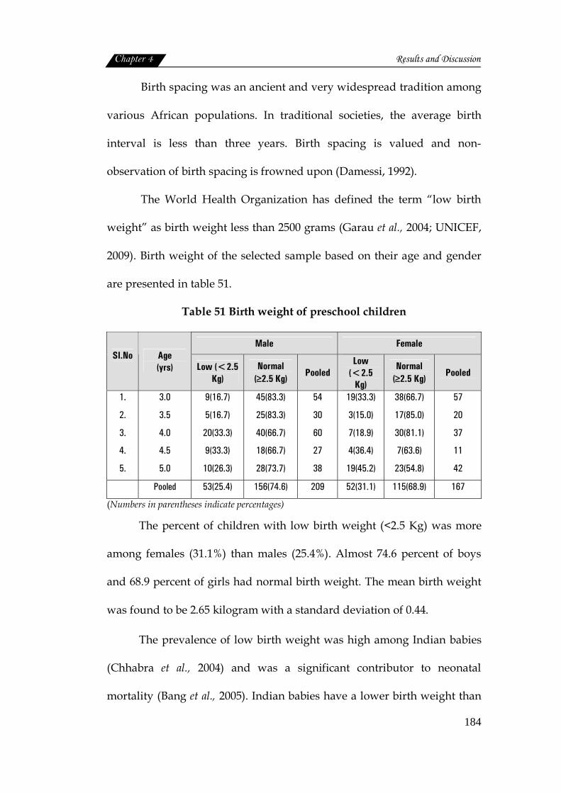
Chapter 4 Results and Discussion
184
Birth spacing was an ancient and very widespread tradition among
various African populations. In traditional societies, the average birth
interval is less than three years. Birth spacing is valued and non-
observation of birth spacing is frowned upon (Damessi, 1992).
The World Health Organization has defined the term “low birth
weight” as birth weight less than 2500 grams (Garau et al., 2004; UNICEF,
2009). Birth weight of the selected sample based on their age and gender
are presented in table 51.
Table 51 Birth weight of preschool children
Male Female Sl.No
Age (yrs) Low (<2.5
Kg) Normal
(≥2.5 Kg) Pooled
Low (<2.5
Kg)
Normal (≥2.5 Kg)
Pooled
1.
2.
3.
4.
5.
3.0
3.5
4.0
4.5
5.0
9(16.7)
5(16.7)
20(33.3)
9(33.3)
10(26.3)
45(83.3)
25(83.3)
40(66.7)
18(66.7)
28(73.7)
54
30
60
27
38
19(33.3)
3(15.0)
7(18.9)
4(36.4)
19(45.2)
38(66.7)
17(85.0)
30(81.1)
7(63.6)
23(54.8)
57
20
37
11
42
Pooled 53(25.4) 156(74.6) 209 52(31.1) 115(68.9) 167
(Numbers in parentheses indicate percentages)
The percent of children with low birth weight (<2.5 Kg) was more
among females (31.1%) than males (25.4%). Almost 74.6 percent of boys
and 68.9 percent of girls had normal birth weight. The mean birth weight
was found to be 2.65 kilogram with a standard deviation of 0.44.
The prevalence of low birth weight was high among Indian babies
(Chhabra et al., 2004) and was a significant contributor to neonatal
mortality (Bang et al., 2005). Indian babies have a lower birth weight than
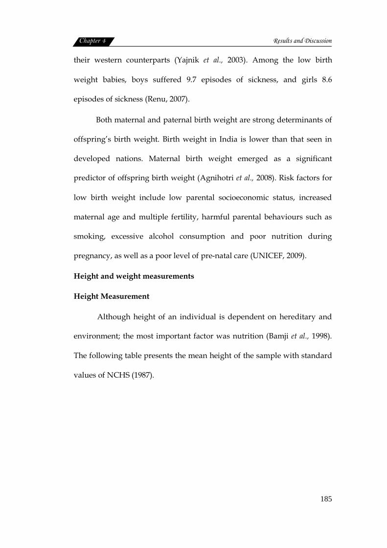
Chapter 4 Results and Discussion
185
their western counterparts (Yajnik et al., 2003). Among the low birth
weight babies, boys suffered 9.7 episodes of sickness, and girls 8.6
episodes of sickness (Renu, 2007).
Both maternal and paternal birth weight are strong determinants of
offspring’s birth weight. Birth weight in India is lower than that seen in
developed nations. Maternal birth weight emerged as a significant
predictor of offspring birth weight (Agnihotri et al., 2008). Risk factors for
low birth weight include low parental socioeconomic status, increased
maternal age and multiple fertility, harmful parental behaviours such as
smoking, excessive alcohol consumption and poor nutrition during
pregnancy, as well as a poor level of pre-natal care (UNICEF, 2009).
Height and weight measurements
Height Measurement
Although height of an individual is dependent on hereditary and
environment; the most important factor was nutrition (Bamji et al., 1998).
The following table presents the mean height of the sample with standard
values of NCHS (1987).
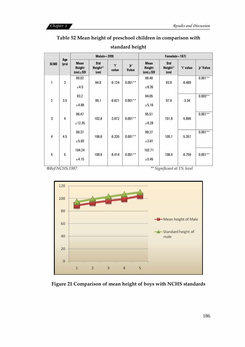
Chapter 4 Results and Discussion
186
Table 52 Mean height of preschool children in comparison with
standard height
Male(n=209) Female(n=167)
Sl.NO Age (yrs) Mean
Height (cm)±SD
Std Height®
(cm)
‘t’ value
‘p’ Value
Mean Height
(cm)±SD
Std Height®
(cm) ‘t’ value ‘p’ Value
1 3 89.02
±4.5 94.6 -9.124 0.001**
88.46
±6.35 93.9 -6.469
0.001**
2 3.5 93.2
±4.88 99.1 -6.621 0.001**
94.05
±5.16 97.9 -3.34
0.003**
3 4 96.47
±12.35 102.8 -3.972 0.001**
95.51
±6.28 101.6 -5.896
0.001**
4 4.5 99.37
±5.93 106.6 -6.335 0.001**
99.27
±3.61 105.1 -5.357
0.001**
5 5 104.24
±4.15 109.9 -8.414 0.001**
102.71
±5.45 108.4 -6.759 0.001**
®Ref:NCHS,1987 ** Significant at 1% level
Figure 21 Comparison of mean height of boys with NCHS standards
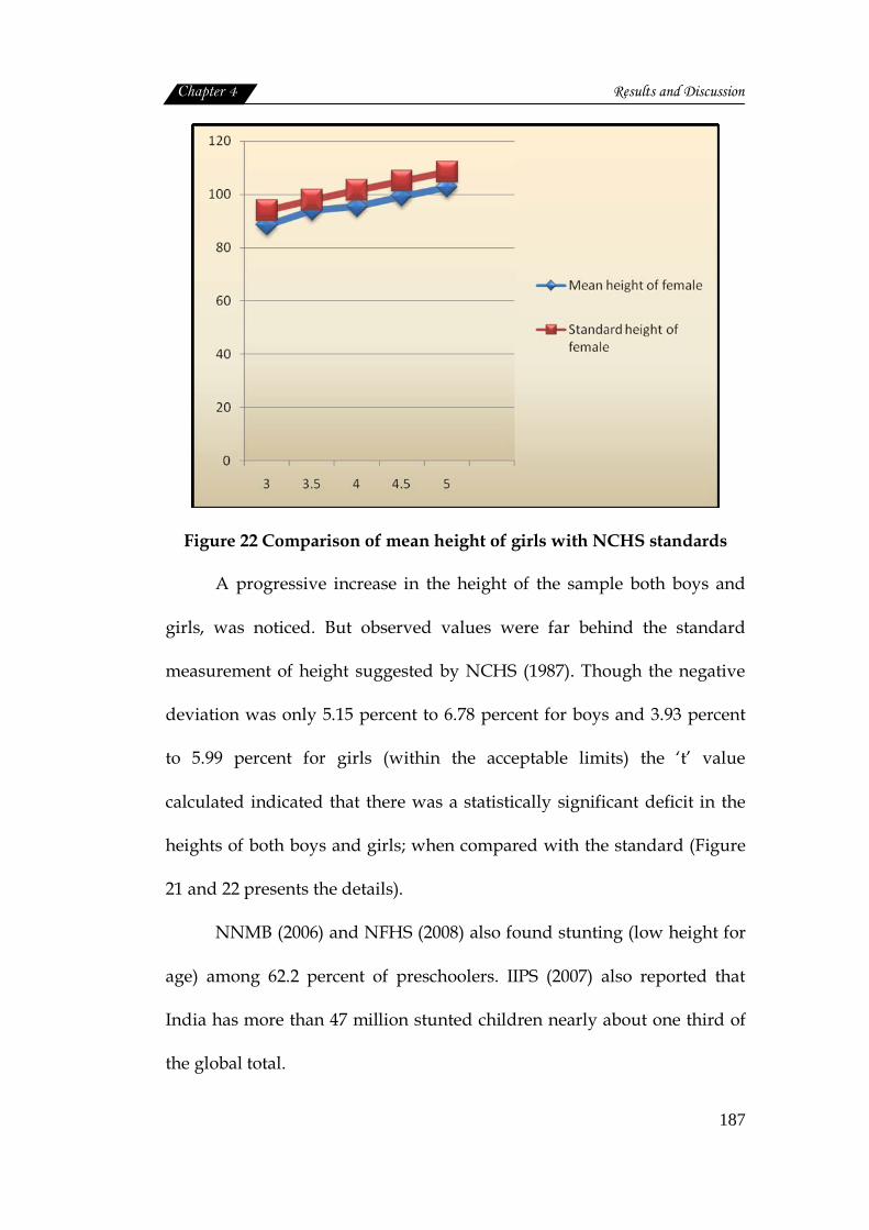
Chapter 4 Results and Discussion
187
Figure 22 Comparison of mean height of girls with NCHS standards
A progressive increase in the height of the sample both boys and
girls, was noticed. But observed values were far behind the standard
measurement of height suggested by NCHS (1987). Though the negative
deviation was only 5.15 percent to 6.78 percent for boys and 3.93 percent
to 5.99 percent for girls (within the acceptable limits) the ‘t’ value
calculated indicated that there was a statistically significant deficit in the
heights of both boys and girls; when compared with the standard (Figure
21 and 22 presents the details).
NNMB (2006) and NFHS (2008) also found stunting (low height for
age) among 62.2 percent of preschoolers. IIPS (2007) also reported that
India has more than 47 million stunted children nearly about one third of
the global total.
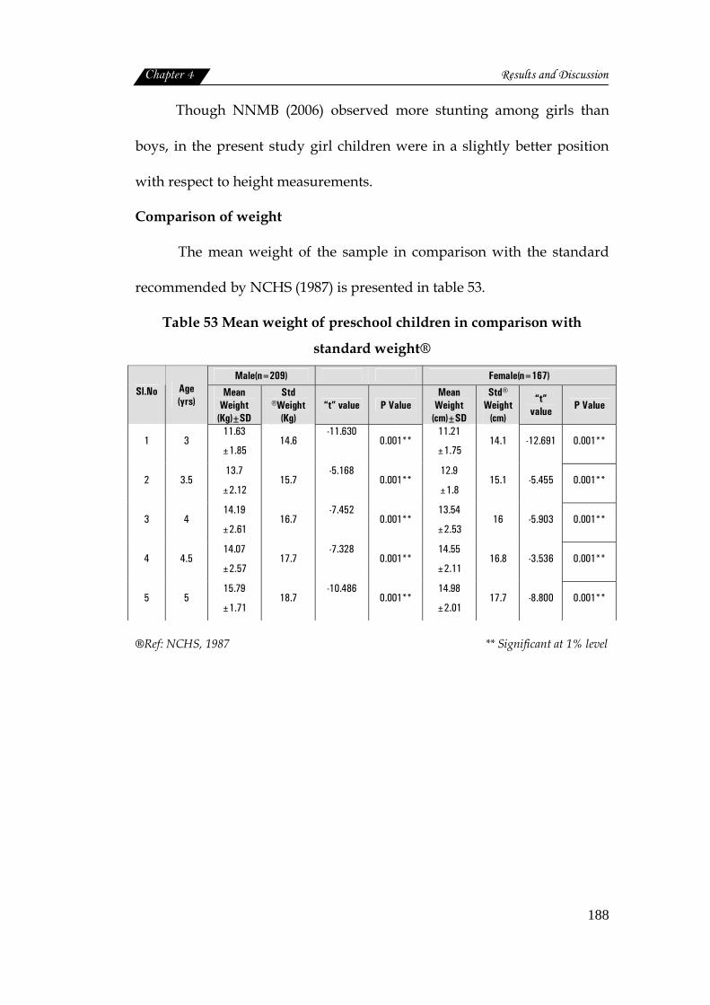
Chapter 4 Results and Discussion
188
Though NNMB (2006) observed more stunting among girls than
boys, in the present study girl children were in a slightly better position
with respect to height measurements.
Comparison of weight
The mean weight of the sample in comparison with the standard
recommended by NCHS (1987) is presented in table 53.
Table 53 Mean weight of preschool children in comparison with
standard weight®
Male(n=209) Female(n=167) Sl.No Age
(yrs) Mean
Weight (Kg)±SD
Std ®Weight
(Kg) “t” value P Value
Mean Weight
(cm)±SD
Std® Weight
(cm)
“t” value P Value
1 3 11.63
±1.85 14.6
-11.630
0.001**
11.21
±1.75 14.1 -12.691 0.001**
2 3.5 13.7
±2.12 15.7
-5.168
0.001**
12.9
±1.8 15.1 -5.455 0.001**
3 4 14.19
±2.61 16.7
-7.452
0.001**
13.54
±2.53 16 -5.903 0.001**
4 4.5 14.07
±2.57 17.7
-7.328
0.001**
14.55
±2.11 16.8 -3.536 0.001**
5 5 15.79
±1.71 18.7
-10.486
0.001**
14.98
±2.01 17.7 -8.800 0.001**
®Ref: NCHS, 1987 ** Significant at 1% level
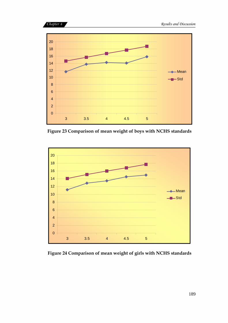
Chapter 4 Results and Discussion
189
0
2
4
6
8
10
12
14
16
18
20
3 3.5 4 4.5 5
Mean
Std
Figure 23 Comparison of mean weight of boys with NCHS standards
0
2
4
6
8
10
12
14
16
18
20
3 3.5 4 4.5 5
Mean
Std
Figure 24 Comparison of mean weight of girls with NCHS standards
Chapter 4 Results and Discussion
190
The mean weight of both boys and girls, although much lower than
the standard values, with a statistical significance at 1 percent level;
showed a progressive increase with age.
However the height deficit found to range between 12.73 percent to
20.5 percent for boys and 13.39 percent to 20.49 percent for girls; indicating
wasting of varying degrees. Severe condition was observed in the 3 year
old boys (20.34%) and girls (20.4%) and 4.5 year old boys (20.5 %). Similar
findings were also reported by Mitra et al.(2007) Figure 23 and 24
illustrates the weight profile of the sample.
Childhood undernutrition remains a major health problem in India,
(Bose et al., 2007). As given by Nandy, et al. (2005) undernutrition
continues to be a primary cause of ill-health and premature mortality
among children in developing countries and chronic undernutrition in
childhood is linked with slower cognitive development and serious health
impairments of later in life that reduce the quality of people (Scrimshaw ,
1996).
Nutritional status based on Gomez classification
Various methods have been suggested to classify children into
various nutritional grades, the most widely used one is the Gomez
classification (Gomez et al., 1956), in which the children are classified as
having first, second or third degree malnutrition if their weight for age
range is 75 to 90 percent, 60 to 75 percent or less than 60 percent
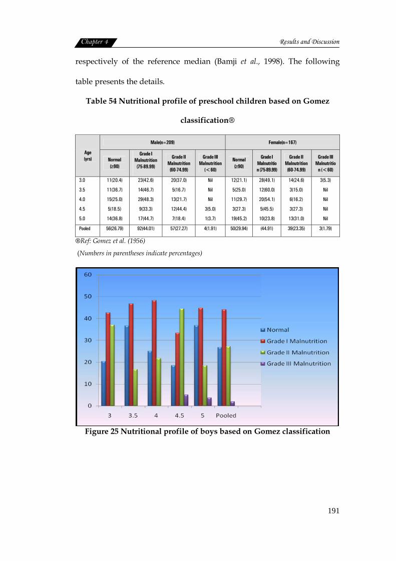
Chapter 4 Results and Discussion
191
respectively of the reference median (Bamji et al., 1998). The following
table presents the details.
Table 54 Nutritional profile of preschool children based on Gomez
classification®
Male(n=209) Female(n=167)
Age (yrs) Normal
(≥90)
Grade I Malnutrition (75-89.99)
Grade II Malnutrition (60-74.99)
Grade III Malnutrition
(<60)
Normal (≥90)
Grade I Malnutrition (75-89.99)
Grade II Malnutrition (60-74.99)
Grade III Malnutritio
n (<60)
3.0
3.5
4.0
4.5
5.0
11(20.4)
11(36.7)
15(25.0)
5(18.5)
14(36.8)
23(42.6)
14(46.7)
29(48.3)
9(33.3)
17(44.7)
20(37.0)
5(16.7)
13(21.7)
12(44.4)
7(18.4)
Nil
Nil
Nil
3(5.0)
1(3.7)
12(21.1)
5(25.0)
11(29.7)
3(27.3)
19(45.2)
28(49.1)
12(60.0)
20(54.1)
5(45.5)
10(23.8)
14(24.6)
3(15.0)
6(16.2)
3(27.3)
13(31.0)
3(5.3)
Nil
Nil
Nil
Nil
Pooled 56(26.79) 92(44.01) 57(27.27) 4(1.91) 50(29.94) (44.91) 39(23.35) 3(1.79)
®Ref: Gomez et al. (1956)
(Numbers in parentheses indicate percentages)
Figure 25 Nutritional profile of boys based on Gomez classification

Chapter 4 Results and Discussion
192
Figure 26 Nutritional profile of girls based on Gomez classification
As per Gomez classification 26.79 percent boys and 29.94 percent of
girls were found to have normal nutritional status. Girls were in a slightly
better position than boys. More number of normal children irrespective of
gender were in the age group of 5 years.
Among the various grades of malnutrition, majority of boys
(44.01%) and girls (44.91%) had Grade I malnutrition followed by Grade II
and Grade III. Here also gender differences was not noticed much.
The rate of prevalence of Grade I malnutrition was uniformly high
in all age groups among boys (33.3% to 48.3%). Almost half of the
population fell under this category. Grade II malnutrition found to occur
among 27.27 percent with highest incidence among 4.5 year age group.
Grade III malnutrition was observed on only 1.91 percent of boys. This
was also noticed among 4.5 to 5 year age group.
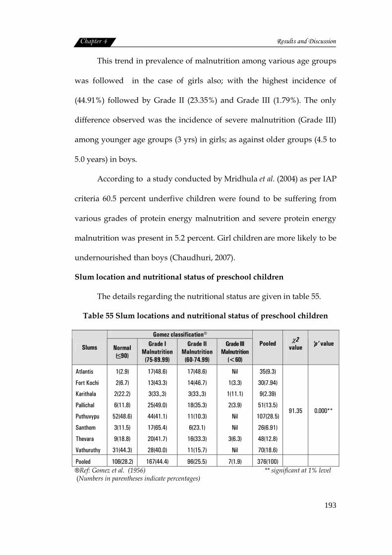
Chapter 4 Results and Discussion
193
This trend in prevalence of malnutrition among various age groups
was followed in the case of girls also; with the highest incidence of
(44.91%) followed by Grade II (23.35%) and Grade III (1.79%). The only
difference observed was the incidence of severe malnutrition (Grade III)
among younger age groups (3 yrs) in girls; as against older groups (4.5 to
5.0 years) in boys.
According to a study conducted by Mridhula et al. (2004) as per IAP
criteria 60.5 percent underfive children were found to be suffering from
various grades of protein energy malnutrition and severe protein energy
malnutrition was present in 5.2 percent. Girl children are more likely to be
undernourished than boys (Chaudhuri, 2007).
Slum location and nutritional status of preschool children
The details regarding the nutritional status are given in table 55.
Table 55 Slum locations and nutritional status of preschool children
Gomez classification®
Slums Normal (≤90)
Grade I Malnutrition
(75-89.99)
Grade II Malnutrition
(60-74.99)
Grade III Malnutrition
(<60)
Pooled
χ2 value
‘p’ value
Atlantis
Fort Kochi
Karithala
Pallichal
Puthuvypu
Santhom
Thevara
Vathuruthy
1(2.9)
2(6.7)
2(22.2)
6(11.8)
52(48.6)
3(11.5)
9(18.8)
31(44.3)
17(48.6)
13(43.3)
3(33.,3)
25(49.0)
44(41.1)
17(65.4)
20(41.7)
28(40.0)
17(48.6)
14(46.7)
3(33.,3)
18(35.3)
11(10.3)
6(23.1)
16(33.3)
11(15.7)
Nil
1(3.3)
1(11.1)
2(3.9)
Nil
Nil
3(6.3)
Nil
35(9.3)
30(7.94)
9(2.39)
51(13.5)
107(28.5)
26(6.91)
48(12.8)
70(18.6)
91.35 0.000**
Pooled 106(28.2) 167(44.4) 96(25.5) 7(1.9) 376(100) ®Ref: Gomez et al. (1956) ** significant at 1% level (Numbers in parentheses indicate percentages)
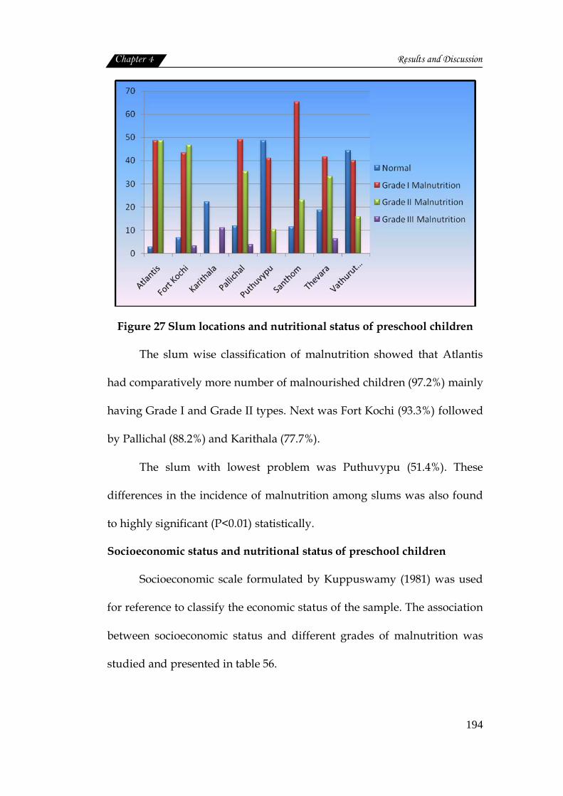
Chapter 4 Results and Discussion
194
Figure 27 Slum locations and nutritional status of preschool children
The slum wise classification of malnutrition showed that Atlantis
had comparatively more number of malnourished children (97.2%) mainly
having Grade I and Grade II types. Next was Fort Kochi (93.3%) followed
by Pallichal (88.2%) and Karithala (77.7%).
The slum with lowest problem was Puthuvypu (51.4%). These
differences in the incidence of malnutrition among slums was also found
to highly significant (P<0.01) statistically.
Socioeconomic status and nutritional status of preschool children
Socioeconomic scale formulated by Kuppuswamy (1981) was used
for reference to classify the economic status of the sample. The association
between socioeconomic status and different grades of malnutrition was
studied and presented in table 56.
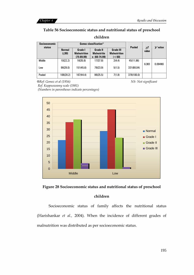
Chapter 4 Results and Discussion
195
Table 56 Socioeconomic status and nutritional status of preschool
children Gomez classification® Socioeconomic
status Normal
(≤90) Grade I
Malnutrition (75-89.99)
Grade II Malnutrition (60-74.99)
Grade III Malnutrition
(<60)
Pooled
χ2
value
‘p’ value
Middle
Low
10(22.2)
96(29.0)
16(35.6)
151(45.6)
17(37.8)
79(23.9)
2(4.4)
5(1.5)
45(11.96)
331(88.04) 6.383 0.094NS
Pooled 106(28.2) 167(44.4) 96(25.5) 7(1.9) 376(100.0)
®Ref: Gomez et al (1956) NS- Not significant Ref. Kuppuswamy scale (1981) (Numbers in parentheses indicate percentages)
0
5
10
15
20
25
30
35
40
45
50
Middle Low
Normal
Grade I
Grade II
Grade III
Figure 28 Socioeconomic status and nutritional status of preschool
children
Socioeconomic status of family affects the nutritional status
(Harishankar et al., 2004). When the incidence of different grades of
malnutrition was distributed as per socioeconomic status.

Chapter 4 Results and Discussion
196
There observed no significant difference. This indicated that
children in both middle and low socioeconomic status were equally
affected by malnutrition. Figure 28 presents the details.
It was also surprising to note that children with normal nutritional
status were more in the low socioeconomic status (29.0%) than the middle
class group (22.2%). So also the Grade II and Grade III malnutrition.
Middle class more affected than the low status group.
Birth order, age, type of family, number of living children, literacy
status of mother and calorie intake were significantly associated with
grades of malnutrition and frequent episodes of infection are also
correlated to stunting (Hassan and Jain, 2009). Children of poor
socioeconomic status group had moderate and severely malnourished
(Elankumaran, 2003). In the present study middle class group was also
equally affected suggesting that the factors other than poverty and poor
access to services play an important role as determinants of under
nutrition in preschool children (Ramachandran, 2007).
Standard of living index and nutritional status of preschool children
The sample was classified based on the standard of living index
(IIPS, 2000). Chi-square analysis was used to find out the association
between nutritional grades and standard of living. The details are
presented in the following table.
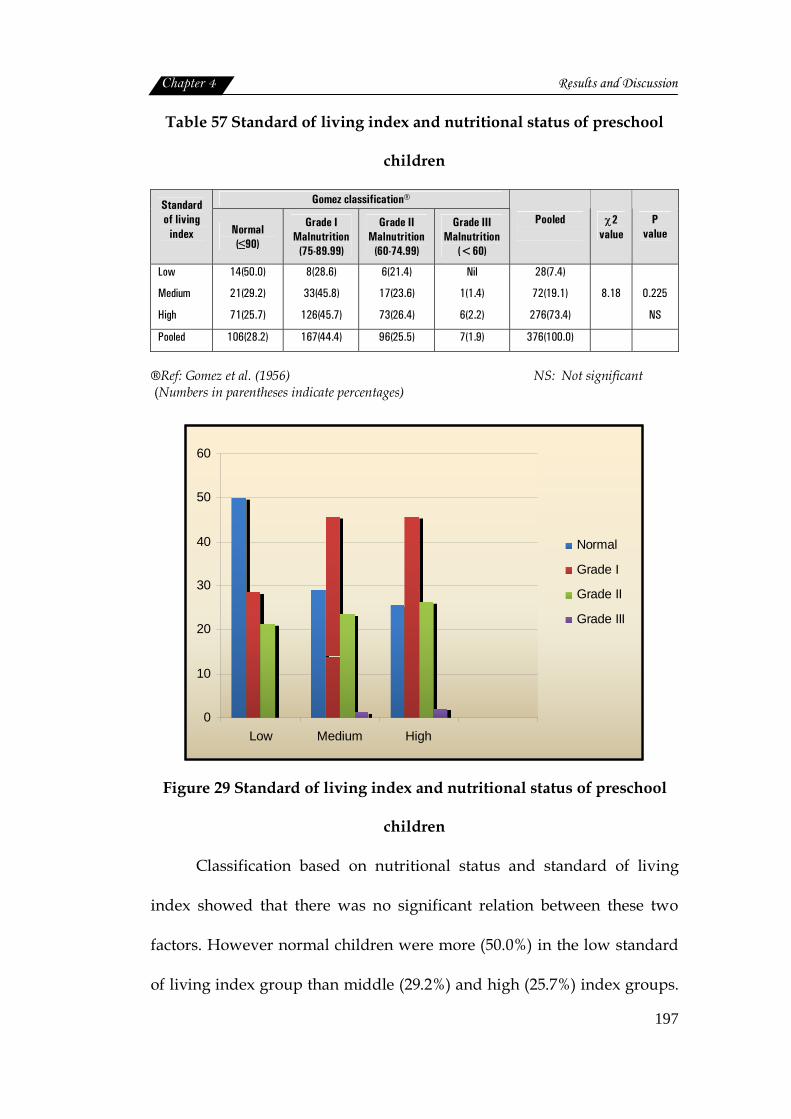
Chapter 4 Results and Discussion
197
Table 57 Standard of living index and nutritional status of preschool
children
Gomez classification® Standard of living
index
Normal (≤90)
Grade I Malnutrition
(75-89.99)
Grade II Malnutrition
(60-74.99)
Grade III Malnutrition
(<60)
Pooled
χ2 value
P value
Low
Medium
High
14(50.0)
21(29.2)
71(25.7)
8(28.6)
33(45.8)
126(45.7)
6(21.4)
17(23.6)
73(26.4)
Nil
1(1.4)
6(2.2)
28(7.4)
72(19.1)
276(73.4)
8.18
0.225
NS
Pooled 106(28.2) 167(44.4) 96(25.5) 7(1.9) 376(100.0)
®Ref: Gomez et al. (1956) NS: Not significant (Numbers in parentheses indicate percentages)
0
10
20
30
40
50
60
Low Medium High
Normal
Grade I
Grade II
Grade III
Figure 29 Standard of living index and nutritional status of preschool
children
Classification based on nutritional status and standard of living
index showed that there was no significant relation between these two
factors. However normal children were more (50.0%) in the low standard
of living index group than middle (29.2%) and high (25.7%) index groups.
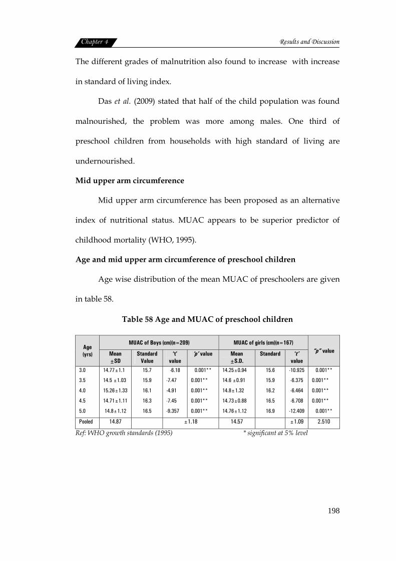
Chapter 4 Results and Discussion
198
The different grades of malnutrition also found to increase with increase
in standard of living index.
Das et al. (2009) stated that half of the child population was found
malnourished, the problem was more among males. One third of
preschool children from households with high standard of living are
undernourished.
Mid upper arm circumference
Mid upper arm circumference has been proposed as an alternative
index of nutritional status. MUAC appears to be superior predictor of
childhood mortality (WHO, 1995).
Age and mid upper arm circumference of preschool children
Age wise distribution of the mean MUAC of preschoolers are given
in table 58.
Table 58 Age and MUAC of preschool children
MUAC of Boys (cm)(n=209) MUAC of girls (cm)(n=167) Age (yrs) Mean
±SD Standard
Value ‘t’
value ‘p’ value Mean
±S.D. Standard
‘t’
value
“p” value
3.0
3.5
4.0
4.5
5.0
14.77±1.1
14.5 ±1.03
15.26±1.33
14.71±1.11
14.8±1.12
15.7
15.9
16.1
16.3
16.5
-6.18
-7.47
-4.91
-7.45
-9.357
0.001**
0.001**
0.001**
0.001**
0.001**
14.25±0.94
14.6 ±0.91
14.8±1.32
14.73±0.88
14.76±1.12
15.6
15.9
16.2
16.5
16.9
-10.925
-6.375
-6.464
-6.708
-12.409
0.001**
0.001**
0.001**
0.001**
0.001**
Pooled 14.87 ±1.18 14.57 ±1.09 2.510
Ref: WHO growth standards (1995) * significant at 5% level
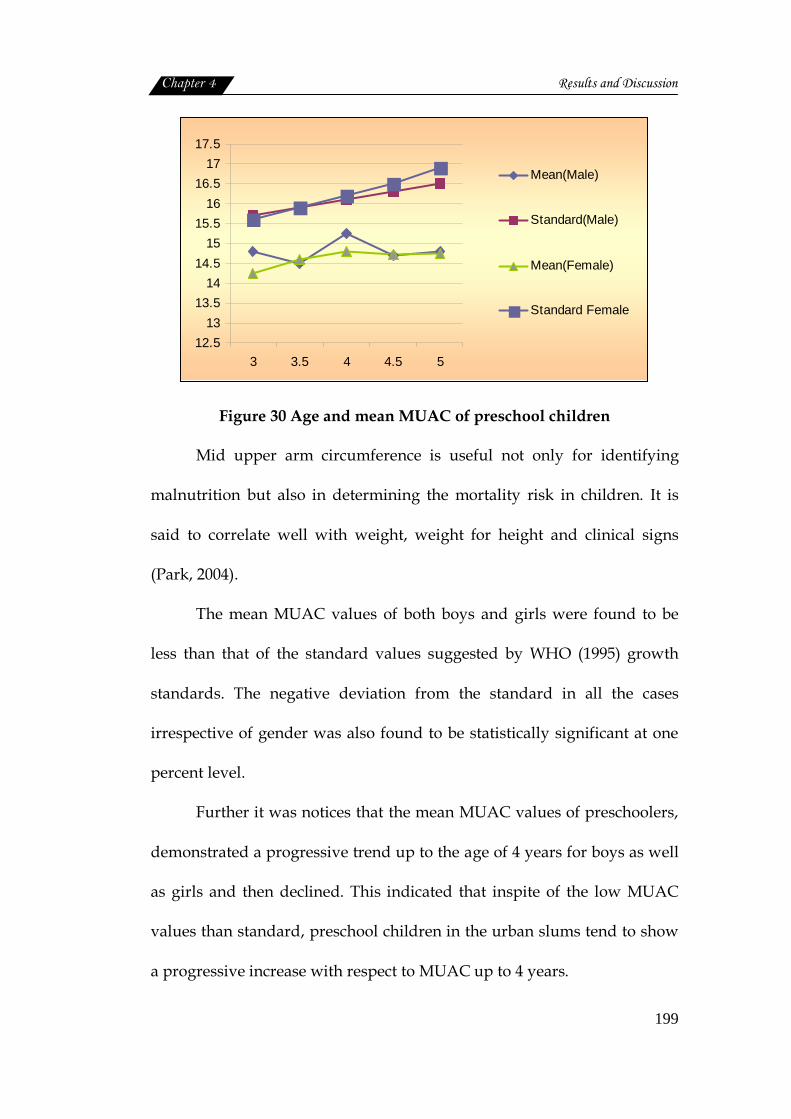
Chapter 4 Results and Discussion
199
12.513
13.514
14.515
15.516
16.517
17.5
3 3.5 4 4.5 5
Mean(Male)
Standard(Male)
Mean(Female)
Standard Female
Figure 30 Age and mean MUAC of preschool children
Mid upper arm circumference is useful not only for identifying
malnutrition but also in determining the mortality risk in children. It is
said to correlate well with weight, weight for height and clinical signs
(Park, 2004).
The mean MUAC values of both boys and girls were found to be
less than that of the standard values suggested by WHO (1995) growth
standards. The negative deviation from the standard in all the cases
irrespective of gender was also found to be statistically significant at one
percent level.
Further it was notices that the mean MUAC values of preschoolers,
demonstrated a progressive trend up to the age of 4 years for boys as well
as girls and then declined. This indicated that inspite of the low MUAC
values than standard, preschool children in the urban slums tend to show
a progressive increase with respect to MUAC up to 4 years.
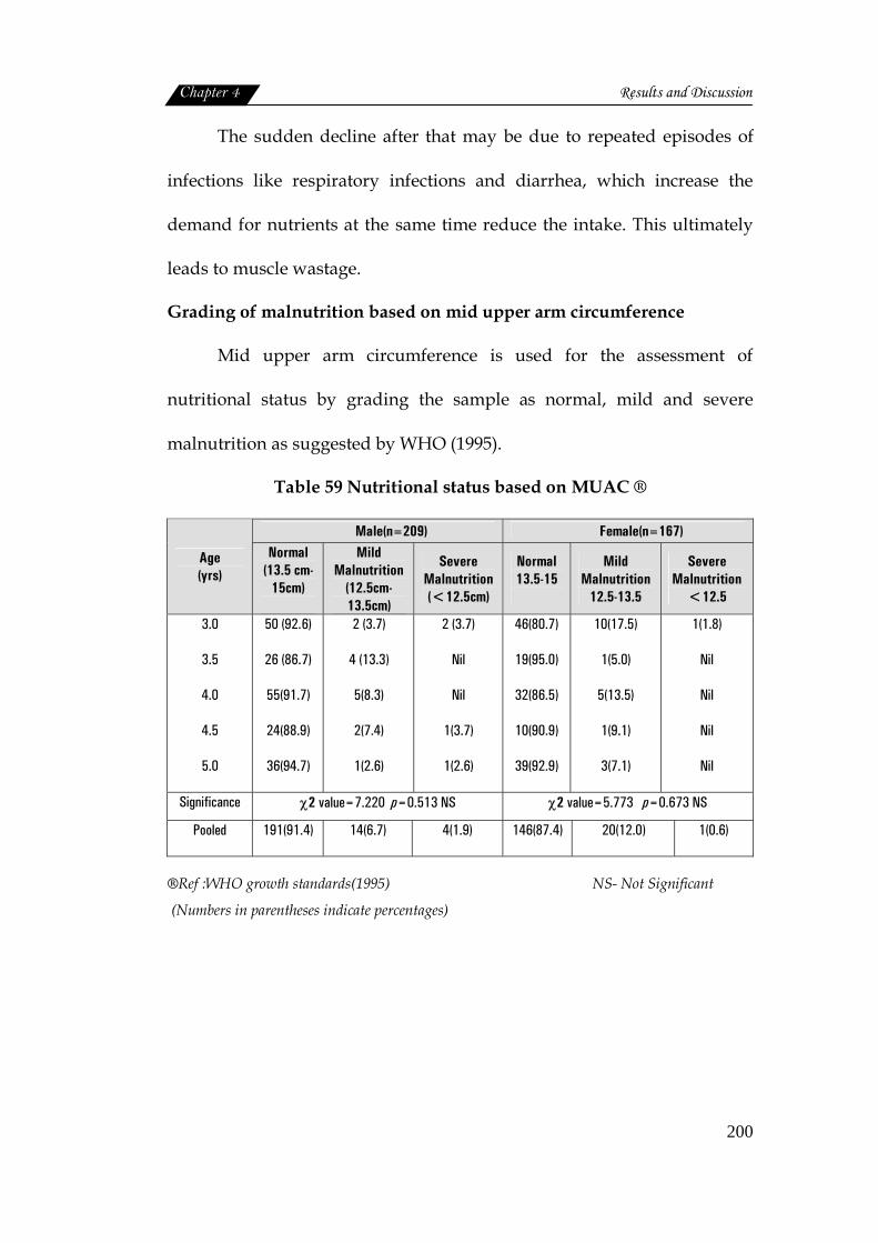
Chapter 4 Results and Discussion
200
The sudden decline after that may be due to repeated episodes of
infections like respiratory infections and diarrhea, which increase the
demand for nutrients at the same time reduce the intake. This ultimately
leads to muscle wastage.
Grading of malnutrition based on mid upper arm circumference
Mid upper arm circumference is used for the assessment of
nutritional status by grading the sample as normal, mild and severe
malnutrition as suggested by WHO (1995).
Table 59 Nutritional status based on MUAC ®
Male(n=209) Female(n=167)
Age (yrs)
Normal (13.5 cm-
15cm)
Mild Malnutrition
(12.5cm-13.5cm)
Severe Malnutrition (<12.5cm)
Normal 13.5-15
Mild Malnutrition
12.5-13.5
Severe Malnutrition
<12.5
3.0
3.5
4.0
4.5
5.0
50 (92.6)
26 (86.7)
55(91.7)
24(88.9)
36(94.7)
2 (3.7)
4 (13.3)
5(8.3)
2(7.4)
1(2.6)
2 (3.7)
Nil
Nil
1(3.7)
1(2.6)
46(80.7)
19(95.0)
32(86.5)
10(90.9)
39(92.9)
10(17.5)
1(5.0)
5(13.5)
1(9.1)
3(7.1)
1(1.8)
Nil
Nil
Nil
Nil
Significance χ2 value=7.220 p=0.513 NS χ2 value=5.773 p=0.673 NS
Pooled 191(91.4) 14(6.7) 4(1.9) 146(87.4) 20(12.0) 1(0.6)
®Ref :WHO growth standards(1995) NS- Not Significant
(Numbers in parentheses indicate percentages)
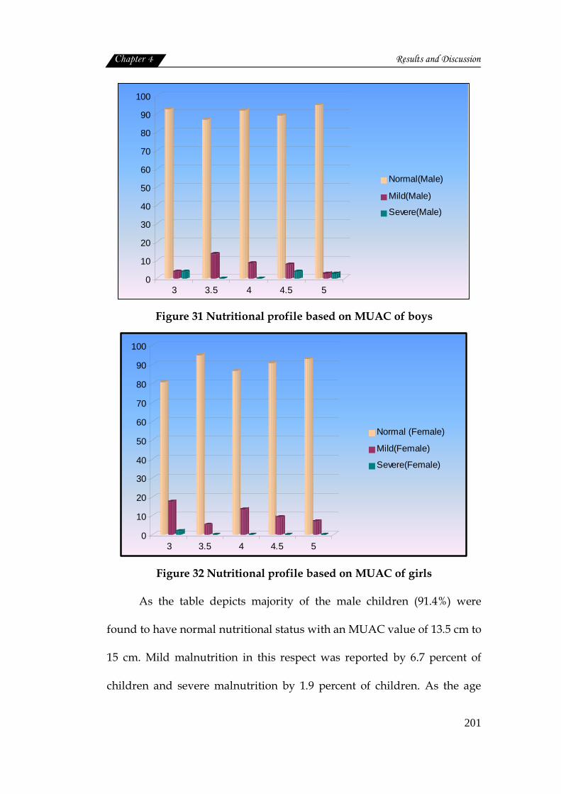
Chapter 4 Results and Discussion
201
0
10
20
30
40
50
60
70
80
90
100
3 3.5 4 4.5 5
Normal(Male)
Mild(Male)
Severe(Male)
Figure 31 Nutritional profile based on MUAC of boys
0
10
20
30
40
50
60
70
80
90
100
3 3.5 4 4.5 5
Normal (Female)
Mild(Female)
Severe(Female)
Figure 32 Nutritional profile based on MUAC of girls
As the table depicts majority of the male children (91.4%) were
found to have normal nutritional status with an MUAC value of 13.5 cm to
15 cm. Mild malnutrition in this respect was reported by 6.7 percent of
children and severe malnutrition by 1.9 percent of children. As the age
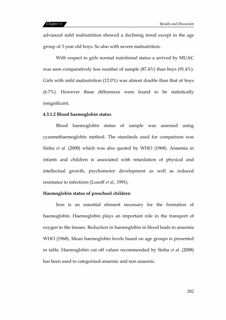
Chapter 4 Results and Discussion
202
advanced mild malnutrition showed a declining trend except in the age
group of 3 year old boys. So also with severe malnutrition.
With respect to girls normal nutritional status a arrived by MUAC
was seen comparatively less number of sample (87.4%) than boys (91.4%).
Girls with mild malnutrition (12.0%) was almost double than that of boys
(6.7%). However these differences were found to be statistically
insignificant.
4.3.1.2 Blood haemoglobin status
Blood haemoglobin status of sample was assessed using
cyanmethaemoglobin method. The standards used for comparison was
Sinha et al. (2008) which was also quoted by WHO (1968). Anaemia in
infants and children is associated with retardation of physical and
intellectual growth, psychomotor development as well as reduced
resistance to infections (Lozoff et al., 1991).
Haemoglobin status of preschool children
Iron is an essential element necessary for the formation of
haemoglobin. Haemoglobin plays an important role in the transport of
oxygen to the tissues. Reduction in haemoglobin in blood leads to anaemia
WHO (1968). Mean haemoglobin levels based on age groups is presented
in table. Haemoglobin cut off values recommended by Sinha et al. (2008)
has been used to categorised anaemic and non anaemic.
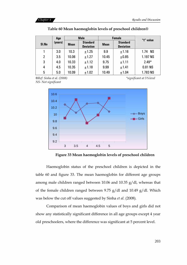
Chapter 4 Results and Discussion
203
Table 60 Mean haemoglobin levels of preschool children®
Male Female Sl.No
Age (years)
Mean Standard Deviation
Mean Standard Deviation
“t” value
1 2 3 4 5
3.0 3.5 4.0 4.5 5.0
10.3 10.06 10.33 10.35 10.09
±1.25 ±1.27 ±1.12 ±1.18 ±1.02
9.9 10.45 9.75 9.99 10.49
±1.16 ±0.85 ±1.11 ±1.41 ±1.04
1.74 NS 1.197 NS
2.49* 0.81 NS
1.783 NS
®Ref: Sinha et al. (2008) *significant at 5%level NS- Not significant
9.2
9.4
9.6
9.8
10
10.2
10.4
10.6
3 3.5 4 4.5 5
Boys
Girls
Figure 33 Mean haemoglobin levels of preschool children
Haemoglobin status of the preschool children is depicted in the
table 60 and figure 33. The mean haemoglobin for different age groups
among male children ranged between 10.06 and 10.35 g/dl, whereas that
of the female children ranged between 9.75 g/dl and 10.49 g/dl. Which
was below the cut off values suggested by Sinha et al. (2008).
Comparison of mean haemoglobin values of boys and girls did not
show any statistically significant difference in all age groups except 4 year
old preschoolers, where the difference was significant at 5 percent level.
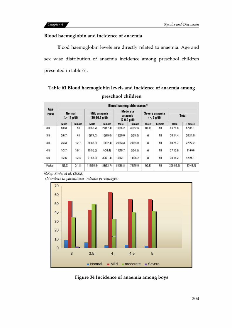
Chapter 4 Results and Discussion
204
Blood haemoglobin and incidence of anaemia
Blood haemoglobin levels are directly related to anaemia. Age and
sex wise distribution of anaemia incidence among preschool children
presented in table 61.
Table 61 Blood haemoglobin levels and incidence of anaemia among
preschool children
Blood haemoglobin status®
Normal (>11 g/dl)
Mild anaemia (10-10.9 g/dl)
Moderate anaemia
(7-9.9 g/dl)
Severe anaemia (<7 g/dl) Total
Age (yrs)
Male Female Male Female Male Female Male Female Male Female
3.0
3.5
4.0
4.5
5.0
5(9.3)
2(6.7)
2(3.3)
1(3.7)
1(2.6)
Nil
Nil
1(2.7)
1(9.1)
1(2.4)
29(53.7)
13(43.,3)
38(63.3)
15(55.6)
21(55.3)
27(47.4)
15(75.0)
12(32.4)
4(36.4)
30(71.4)
19(35.2)
15(50.0)
20(33.3)
11(40.7)
16(42.1)
30(52.6)
5(25.0)
24(64.9)
6(54.5)
11(26.2)
1(1.9)
Nil
Nil
Nil
Nil
Nil
Nil
Nil
Nil
Nil
54(25.8)
30(14.4)
60(28.7)
27(12.9)
38(18.2)
57(34.1)
20(11.9)
37(22.2)
11(6.6)
42(25.1)
Pooled 11(5.3) 3(1.8) 116(55.5) 88(52.7) 81(38.8) 76(45.5) 1(0.5) Nil 209(55.6) 167(44.4)
®Ref: Sinha et al. (2008) (Numbers in parentheses indicate percentages)
0
10
20
30
40
50
60
70
3 3.5 4 4.5 5
Normal Mild moderate Severe
Figure 34 Incidence of anaemia among boys
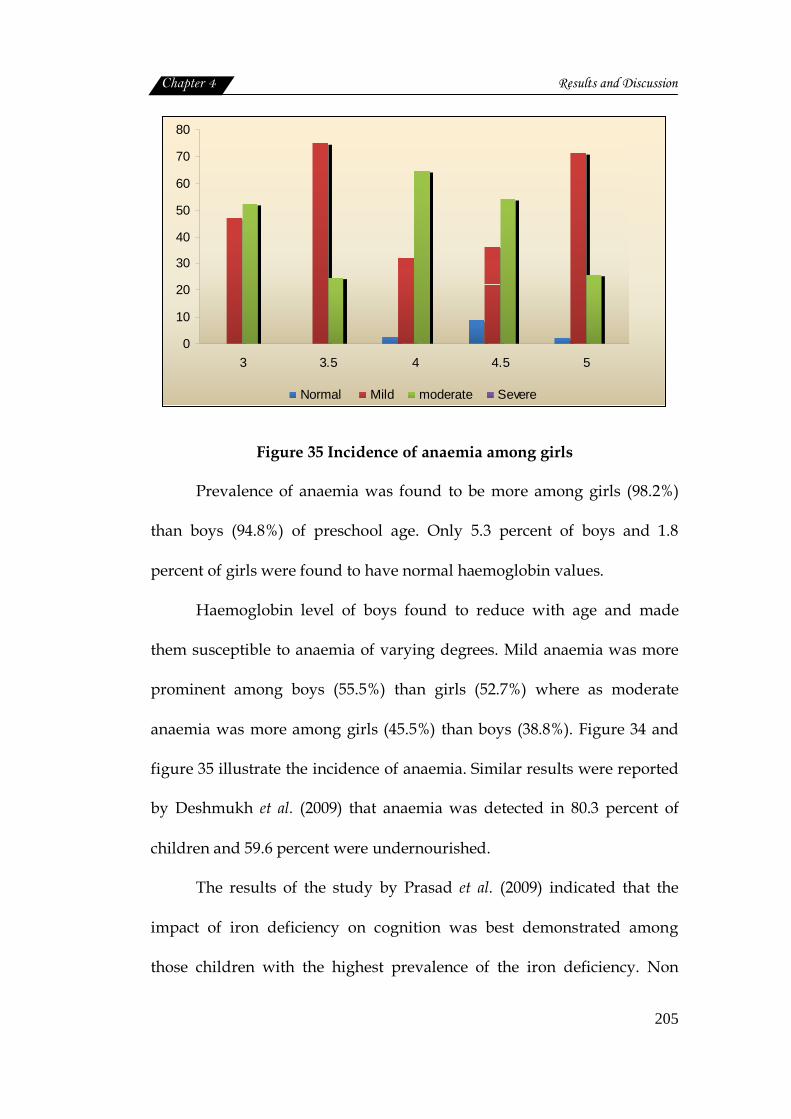
Chapter 4 Results and Discussion
205
0
10
20
30
40
50
60
70
80
3 3.5 4 4.5 5
Normal Mild moderate Severe
Figure 35 Incidence of anaemia among girls
Prevalence of anaemia was found to be more among girls (98.2%)
than boys (94.8%) of preschool age. Only 5.3 percent of boys and 1.8
percent of girls were found to have normal haemoglobin values.
Haemoglobin level of boys found to reduce with age and made
them susceptible to anaemia of varying degrees. Mild anaemia was more
prominent among boys (55.5%) than girls (52.7%) where as moderate
anaemia was more among girls (45.5%) than boys (38.8%). Figure 34 and
figure 35 illustrate the incidence of anaemia. Similar results were reported
by Deshmukh et al. (2009) that anaemia was detected in 80.3 percent of
children and 59.6 percent were undernourished.
The results of the study by Prasad et al. (2009) indicated that the
impact of iron deficiency on cognition was best demonstrated among
those children with the highest prevalence of the iron deficiency. Non
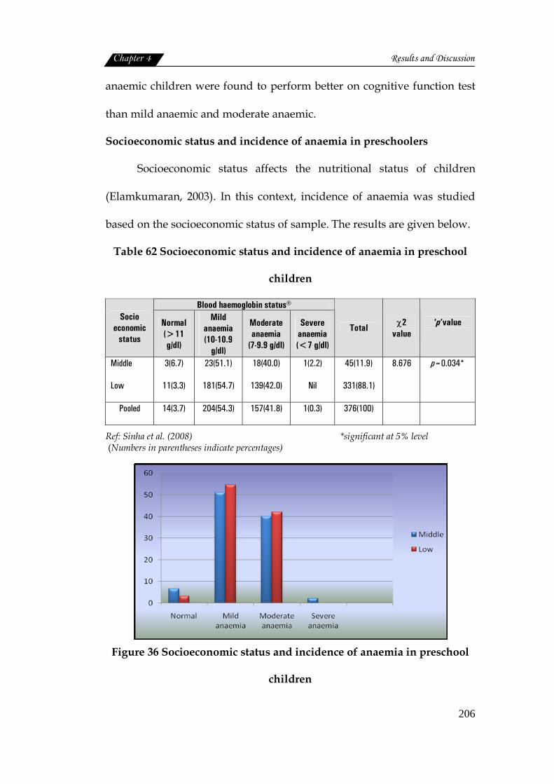
Chapter 4 Results and Discussion
206
anaemic children were found to perform better on cognitive function test
than mild anaemic and moderate anaemic.
Socioeconomic status and incidence of anaemia in preschoolers
Socioeconomic status affects the nutritional status of children
(Elamkumaran, 2003). In this context, incidence of anaemia was studied
based on the socioeconomic status of sample. The results are given below.
Table 62 Socioeconomic status and incidence of anaemia in preschool
children
Blood haemoglobin status® Socio
economic status
Normal (>11 g/dl)
Mild anaemia (10-10.9
g/dl)
Moderate anaemia
(7-9.9 g/dl)
Severe anaemia (<7 g/dl)
Total χ2 value
‘p’value
Middle
Low
3(6.7)
11(3.3)
23(51.1)
181(54.7)
18(40.0)
139(42.0)
1(2.2)
Nil
45(11.9)
331(88.1)
8.676
p=0.034*
Pooled 14(3.7) 204(54.3) 157(41.8) 1(0.3) 376(100)
Ref: Sinha et al. (2008) *significant at 5% level (Numbers in parentheses indicate percentages)
Figure 36 Socioeconomic status and incidence of anaemia in preschool
children
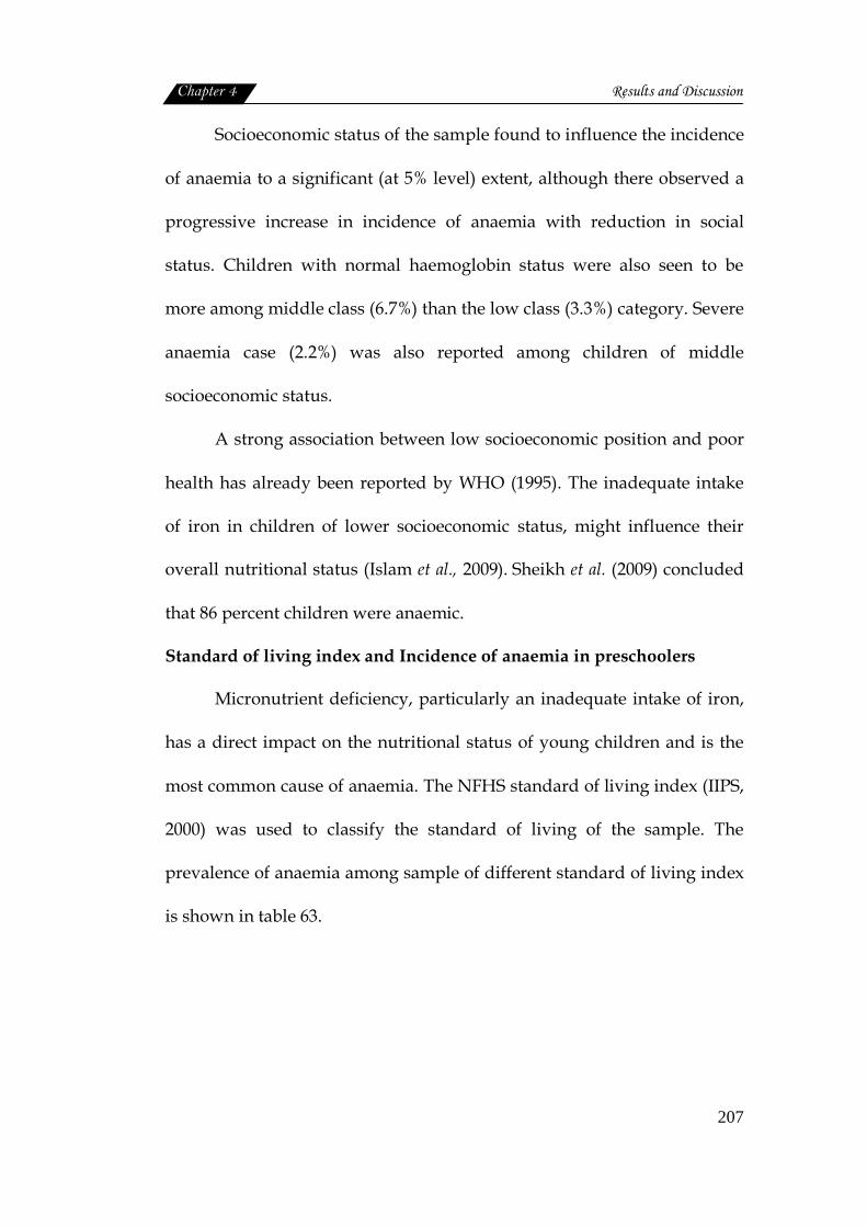
Chapter 4 Results and Discussion
207
Socioeconomic status of the sample found to influence the incidence
of anaemia to a significant (at 5% level) extent, although there observed a
progressive increase in incidence of anaemia with reduction in social
status. Children with normal haemoglobin status were also seen to be
more among middle class (6.7%) than the low class (3.3%) category. Severe
anaemia case (2.2%) was also reported among children of middle
socioeconomic status.
A strong association between low socioeconomic position and poor
health has already been reported by WHO (1995). The inadequate intake
of iron in children of lower socioeconomic status, might influence their
overall nutritional status (Islam et al., 2009). Sheikh et al. (2009) concluded
that 86 percent children were anaemic.
Standard of living index and Incidence of anaemia in preschoolers
Micronutrient deficiency, particularly an inadequate intake of iron,
has a direct impact on the nutritional status of young children and is the
most common cause of anaemia. The NFHS standard of living index (IIPS,
2000) was used to classify the standard of living of the sample. The
prevalence of anaemia among sample of different standard of living index
is shown in table 63.
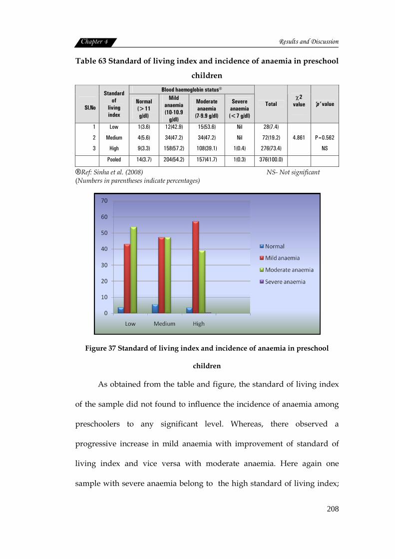
Chapter 4 Results and Discussion
208
Table 63 Standard of living index and incidence of anaemia in preschool
children
Blood haemoglobin status®
Sl.No
Standard of
living index
Normal (>11 g/dl)
Mild anaemia (10-10.9
g/dl)
Moderate anaemia
(7-9.9 g/dl)
Severe anaemia (<7 g/dl)
Total χ2
value
‘p’ value
1
2
3
Low
Medium
High
1(3.6)
4(5.6)
9(3.3)
12(42.9)
34(47.2)
158(57.2)
15(53.6)
34(47.2)
108(39.1)
Nil
Nil
1(0.4)
28(7.4)
72(19.2)
276(73.4)
4.861
P=0.562
NS
Pooled 14(3.7) 204(54.2) 157(41.7) 1(0.3) 376(100.0)
®Ref: Sinha et al. (2008) NS- Not significant (Numbers in parentheses indicate percentages)
Figure 37 Standard of living index and incidence of anaemia in preschool
children
As obtained from the table and figure, the standard of living index
of the sample did not found to influence the incidence of anaemia among
preschoolers to any significant level. Whereas, there observed a
progressive increase in mild anaemia with improvement of standard of
living index and vice versa with moderate anaemia. Here again one
sample with severe anaemia belong to the high standard of living index;
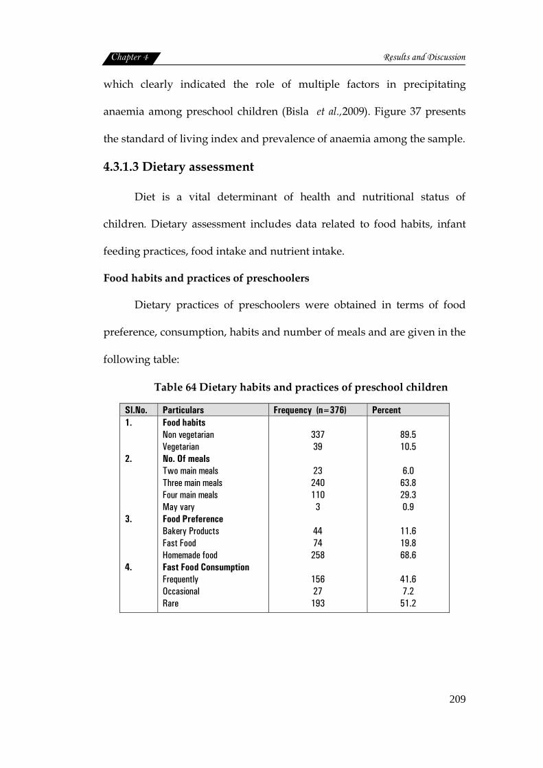
Chapter 4 Results and Discussion
209
which clearly indicated the role of multiple factors in precipitating
anaemia among preschool children (Bisla et al.,2009). Figure 37 presents
the standard of living index and prevalence of anaemia among the sample.
4.3.1.3 Dietary assessment
Diet is a vital determinant of health and nutritional status of
children. Dietary assessment includes data related to food habits, infant
feeding practices, food intake and nutrient intake.
Food habits and practices of preschoolers
Dietary practices of preschoolers were obtained in terms of food
preference, consumption, habits and number of meals and are given in the
following table:
Table 64 Dietary habits and practices of preschool children
Sl.No. Particulars Frequency (n=376) Percent 1. 2. 3. 4.
Food habits Non vegetarian Vegetarian No. Of meals Two main meals Three main meals Four main meals May vary Food Preference Bakery Products Fast Food Homemade food Fast Food Consumption Frequently Occasional Rare
337 39
23 240 110
3
44 74 258
156 27 193
89.5 10.5
6.0
63.8 29.3 0.9
11.6 19.8 68.6
41.6 7.2
51.2
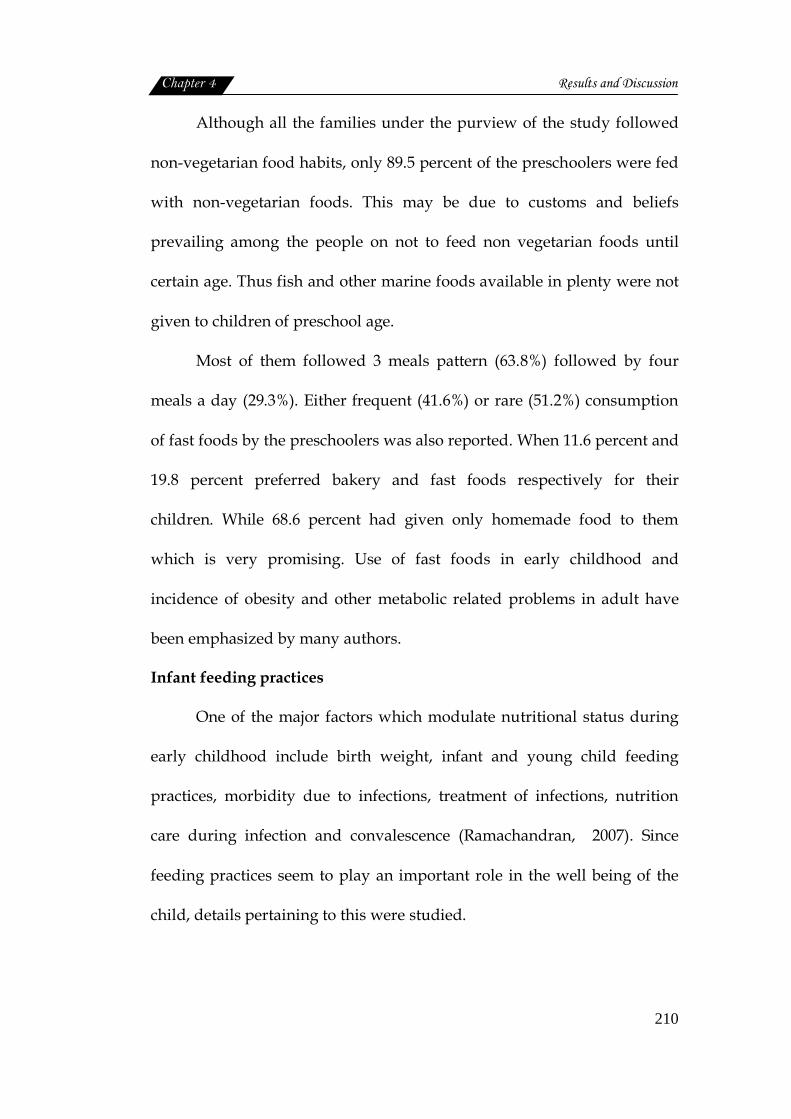
Chapter 4 Results and Discussion
210
Although all the families under the purview of the study followed
non-vegetarian food habits, only 89.5 percent of the preschoolers were fed
with non-vegetarian foods. This may be due to customs and beliefs
prevailing among the people on not to feed non vegetarian foods until
certain age. Thus fish and other marine foods available in plenty were not
given to children of preschool age.
Most of them followed 3 meals pattern (63.8%) followed by four
meals a day (29.3%). Either frequent (41.6%) or rare (51.2%) consumption
of fast foods by the preschoolers was also reported. When 11.6 percent and
19.8 percent preferred bakery and fast foods respectively for their
children. While 68.6 percent had given only homemade food to them
which is very promising. Use of fast foods in early childhood and
incidence of obesity and other metabolic related problems in adult have
been emphasized by many authors.
Infant feeding practices
One of the major factors which modulate nutritional status during
early childhood include birth weight, infant and young child feeding
practices, morbidity due to infections, treatment of infections, nutrition
care during infection and convalescence (Ramachandran, 2007). Since
feeding practices seem to play an important role in the well being of the
child, details pertaining to this were studied.
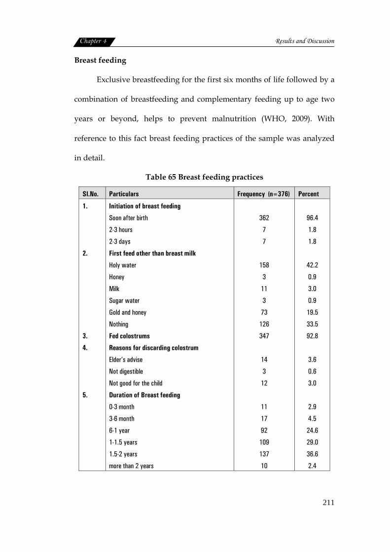
Chapter 4 Results and Discussion
211
Breast feeding
Exclusive breastfeeding for the first six months of life followed by a
combination of breastfeeding and complementary feeding up to age two
years or beyond, helps to prevent malnutrition (WHO, 2009). With
reference to this fact breast feeding practices of the sample was analyzed
in detail.
Table 65 Breast feeding practices
Sl.No. Particulars Frequency (n=376) Percent
1.
2.
3.
4.
5.
Initiation of breast feeding
Soon after birth
2-3 hours
2-3 days
First feed other than breast milk
Holy water
Honey
Milk
Sugar water
Gold and honey
Nothing
Fed colostrums
Reasons for discarding colostrum
Elder’s advise
Not digestible
Not good for the child
Duration of Breast feeding
0-3 month
3-6 month
6-1 year
1-1.5 years
1.5-2 years
more than 2 years
362
7
7
158
3
11
3
73
126
347
14
3
12
11
17
92
109
137
10
96.4
1.8
1.8
42.2
0.9
3.0
0.9
19.5
33.5
92.8
3.6
0.6
3.0
2.9
4.5
24.6
29.0
36.6
2.4
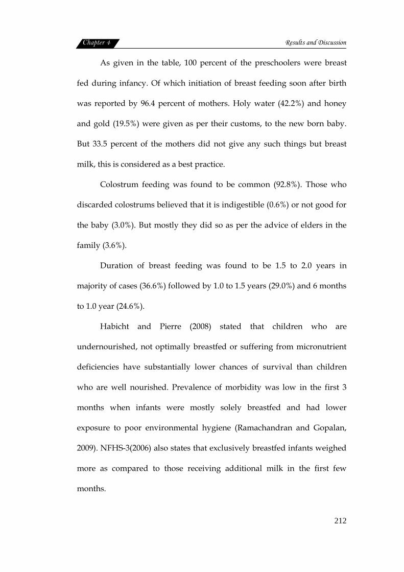
Chapter 4 Results and Discussion
212
As given in the table, 100 percent of the preschoolers were breast
fed during infancy. Of which initiation of breast feeding soon after birth
was reported by 96.4 percent of mothers. Holy water (42.2%) and honey
and gold (19.5%) were given as per their customs, to the new born baby.
But 33.5 percent of the mothers did not give any such things but breast
milk, this is considered as a best practice.
Colostrum feeding was found to be common (92.8%). Those who
discarded colostrums believed that it is indigestible (0.6%) or not good for
the baby (3.0%). But mostly they did so as per the advice of elders in the
family (3.6%).
Duration of breast feeding was found to be 1.5 to 2.0 years in
majority of cases (36.6%) followed by 1.0 to 1.5 years (29.0%) and 6 months
to 1.0 year (24.6%).
Habicht and Pierre (2008) stated that children who are
undernourished, not optimally breastfed or suffering from micronutrient
deficiencies have substantially lower chances of survival than children
who are well nourished. Prevalence of morbidity was low in the first 3
months when infants were mostly solely breastfed and had lower
exposure to poor environmental hygiene (Ramachandran and Gopalan,
2009). NFHS-3(2006) also states that exclusively breastfed infants weighed
more as compared to those receiving additional milk in the first few
months.
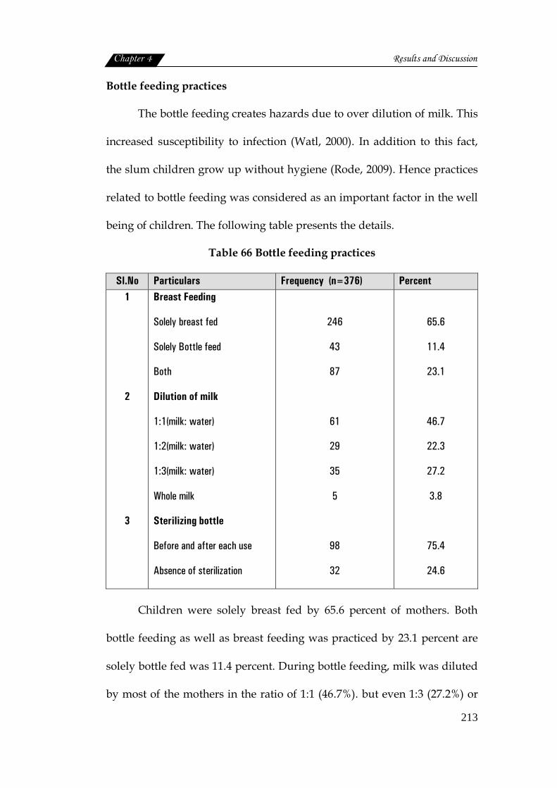
Chapter 4 Results and Discussion
213
Bottle feeding practices
The bottle feeding creates hazards due to over dilution of milk. This
increased susceptibility to infection (Watl, 2000). In addition to this fact,
the slum children grow up without hygiene (Rode, 2009). Hence practices
related to bottle feeding was considered as an important factor in the well
being of children. The following table presents the details.
Table 66 Bottle feeding practices
Sl.No Particulars Frequency (n=376) Percent 1
2
3
Breast Feeding
Solely breast fed
Solely Bottle feed
Both
Dilution of milk
1:1(milk: water)
1:2(milk: water)
1:3(milk: water)
Whole milk
Sterilizing bottle
Before and after each use
Absence of sterilization
246
43
87
61
29
35
5
98
32
65.6
11.4
23.1
46.7
22.3
27.2
3.8
75.4
24.6
Children were solely breast fed by 65.6 percent of mothers. Both
bottle feeding as well as breast feeding was practiced by 23.1 percent are
solely bottle fed was 11.4 percent. During bottle feeding, milk was diluted
by most of the mothers in the ratio of 1:1 (46.7%). but even 1:3 (27.2%) or
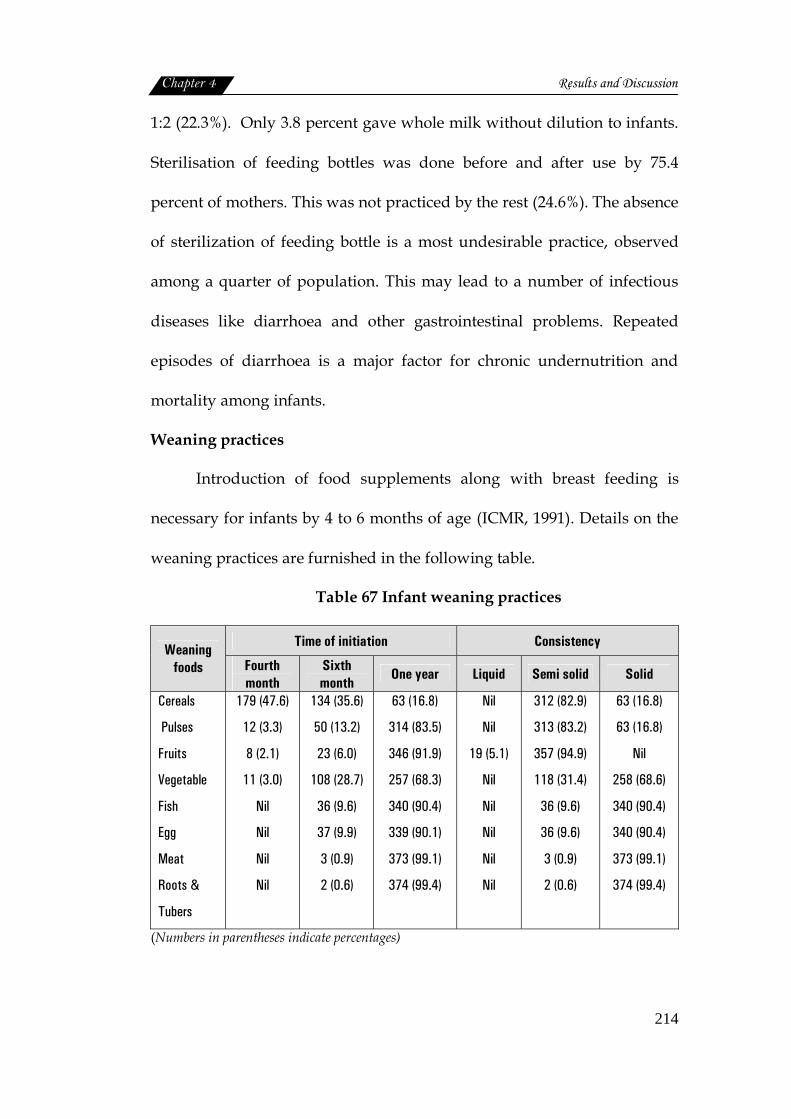
Chapter 4 Results and Discussion
214
1:2 (22.3%). Only 3.8 percent gave whole milk without dilution to infants.
Sterilisation of feeding bottles was done before and after use by 75.4
percent of mothers. This was not practiced by the rest (24.6%). The absence
of sterilization of feeding bottle is a most undesirable practice, observed
among a quarter of population. This may lead to a number of infectious
diseases like diarrhoea and other gastrointestinal problems. Repeated
episodes of diarrhoea is a major factor for chronic undernutrition and
mortality among infants.
Weaning practices
Introduction of food supplements along with breast feeding is
necessary for infants by 4 to 6 months of age (ICMR, 1991). Details on the
weaning practices are furnished in the following table.
Table 67 Infant weaning practices
Time of initiation Consistency Weaning foods Fourth
month Sixth month
One year Liquid Semi solid Solid
Cereals
Pulses
Fruits
Vegetable
Fish
Egg
Meat
Roots &
Tubers
179 (47.6)
12 (3.3)
8 (2.1)
11 (3.0)
Nil
Nil
Nil
Nil
134 (35.6)
50 (13.2)
23 (6.0)
108 (28.7)
36 (9.6)
37 (9.9)
3 (0.9)
2 (0.6)
63 (16.8)
314 (83.5)
346 (91.9)
257 (68.3)
340 (90.4)
339 (90.1)
373 (99.1)
374 (99.4)
Nil
Nil
19 (5.1)
Nil
Nil
Nil
Nil
Nil
312 (82.9)
313 (83.2)
357 (94.9)
118 (31.4)
36 (9.6)
36 (9.6)
3 (0.9)
2 (0.6)
63 (16.8)
63 (16.8)
Nil
258 (68.6)
340 (90.4)
340 (90.4)
373 (99.1)
374 (99.4)
(Numbers in parentheses indicate percentages)
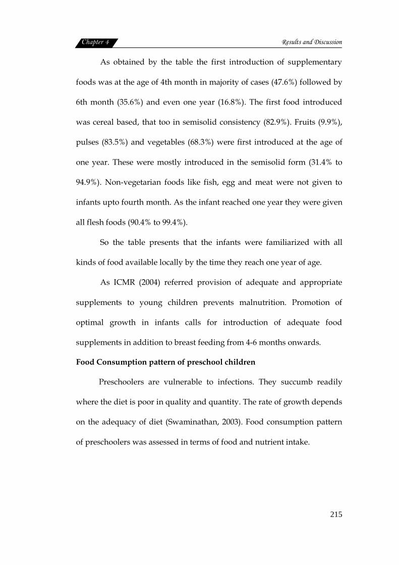
Chapter 4 Results and Discussion
215
As obtained by the table the first introduction of supplementary
foods was at the age of 4th month in majority of cases (47.6%) followed by
6th month (35.6%) and even one year (16.8%). The first food introduced
was cereal based, that too in semisolid consistency (82.9%). Fruits (9.9%),
pulses (83.5%) and vegetables (68.3%) were first introduced at the age of
one year. These were mostly introduced in the semisolid form (31.4% to
94.9%). Non-vegetarian foods like fish, egg and meat were not given to
infants upto fourth month. As the infant reached one year they were given
all flesh foods (90.4% to 99.4%).
So the table presents that the infants were familiarized with all
kinds of food available locally by the time they reach one year of age.
As ICMR (2004) referred provision of adequate and appropriate
supplements to young children prevents malnutrition. Promotion of
optimal growth in infants calls for introduction of adequate food
supplements in addition to breast feeding from 4-6 months onwards.
Food Consumption pattern of preschool children
Preschoolers are vulnerable to infections. They succumb readily
where the diet is poor in quality and quantity. The rate of growth depends
on the adequacy of diet (Swaminathan, 2003). Food consumption pattern
of preschoolers was assessed in terms of food and nutrient intake.
Chapter 4 Results and Discussion
216
Mean food intake in comparison with RDA
The mean food intake of preschoolers in comparison with
recommended dietary allowances specified by ICMR (2004) is shown in
the following table.
Table 68 Mean food intake of preschool children in comparison with RDA®
Food Items RDA (g)
Mean Intake(g)
Standard Devaition
Mean difference
Std Error
“t” value ‘p’ value
Cereals
Pulses
GLV
Other vegetables
Roots
Fruits
Milk
Fats &oil
Fish &meat
Egg
Sugar
200
50
75
50
50
50
200
25
30
30
40
160.7 (-19.7)
13.7 (-72.6)
0.8 (-98.93)
34.7 (-30.6)
5.7 (-88.6)
7.7 (-84.6)
77.7(-61.15)
29.7(+18.8)
56.7 (+89.0)
8.3 (-72.33)
17.5 (-56.25)
±31.24
±17.85
±3.239
±36.48
±9.625
±20.28
±2.24
±8.401
±30.83
±18.95
±4.69
-39.3
-36.3
-74.2
-15.3
-44.3
-42.3
-122.3
4.7
26.7
-21.7
-22.5
5.705
3.260
0.591
6.661
1.757
3.704
7.712
1.534
5.629
3.460
0.856
-6.889
-11.145
-125.433
-2.302
-25.228
-11.229
-15.864
3.043
4.737
-6.262
-26.285
0.000**
0.000**
0.000**
0.029*
0.000**
0.000**
0.000**
0.005**
0.000**
0.000**
0.000** ®Ref : ICMR(2004) ** Significant at 1% level (Numbers in parentheses indicate percentage adequacy) *Significant at 5% level
Figure 38 Comparison of mean food intake of preschool children with
RDA
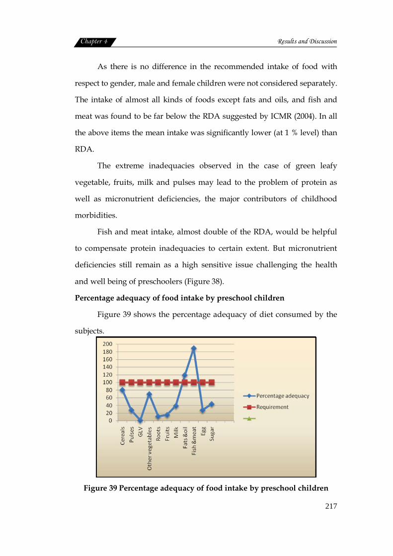
Chapter 4 Results and Discussion
217
As there is no difference in the recommended intake of food with
respect to gender, male and female children were not considered separately.
The intake of almost all kinds of foods except fats and oils, and fish and
meat was found to be far below the RDA suggested by ICMR (2004). In all
the above items the mean intake was significantly lower (at 1 % level) than
RDA.
The extreme inadequacies observed in the case of green leafy
vegetable, fruits, milk and pulses may lead to the problem of protein as
well as micronutrient deficiencies, the major contributors of childhood
morbidities.
Fish and meat intake, almost double of the RDA, would be helpful
to compensate protein inadequacies to certain extent. But micronutrient
deficiencies still remain as a high sensitive issue challenging the health
and well being of preschoolers (Figure 38).
Percentage adequacy of food intake by preschool children
Figure 39 shows the percentage adequacy of diet consumed by the
subjects.
Figure 39 Percentage adequacy of food intake by preschool children
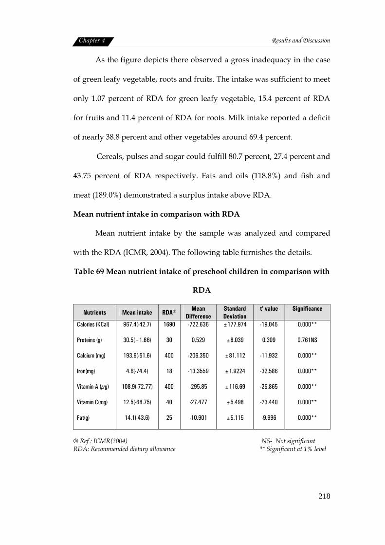
Chapter 4 Results and Discussion
218
As the figure depicts there observed a gross inadequacy in the case
of green leafy vegetable, roots and fruits. The intake was sufficient to meet
only 1.07 percent of RDA for green leafy vegetable, 15.4 percent of RDA
for fruits and 11.4 percent of RDA for roots. Milk intake reported a deficit
of nearly 38.8 percent and other vegetables around 69.4 percent.
Cereals, pulses and sugar could fulfill 80.7 percent, 27.4 percent and
43.75 percent of RDA respectively. Fats and oils (118.8%) and fish and
meat (189.0%) demonstrated a surplus intake above RDA.
Mean nutrient intake in comparison with RDA
Mean nutrient intake by the sample was analyzed and compared
with the RDA (ICMR, 2004). The following table furnishes the details.
Table 69 Mean nutrient intake of preschool children in comparison with
RDA
Nutrients Mean intake RDA® Mean Difference
Standard Deviation
t’ value
Significance
Calories (KCal)
Proteins (g)
Calcium (mg)
Iron(mg)
Vitamin A (µg)
Vitamin C(mg)
Fat(g)
967.4(-42.7)
30.5(+1.66)
193.6(-51.6)
4.6(-74.4)
108.9(-72.77)
12.5(-68.75)
14.1(-43.6)
1690
30
400
18
400
40
25
-722.636
0.529
-206.350
-13.3559
-295.85
-27.477
-10.901
±177.974
±8.039
±81.112
±1.9224
±116.69
±5.498
±5.115
-19.045
0.309
-11.932
-32.586
-25.865
-23.440
-9.996
0.000**
0.761NS
0.000**
0.000**
0.000**
0.000**
0.000**
® Ref : ICMR(2004) NS- Not significant RDA: Recommended dietary allowance ** Significant at 1% level
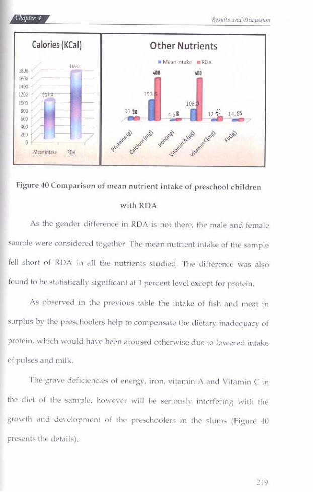
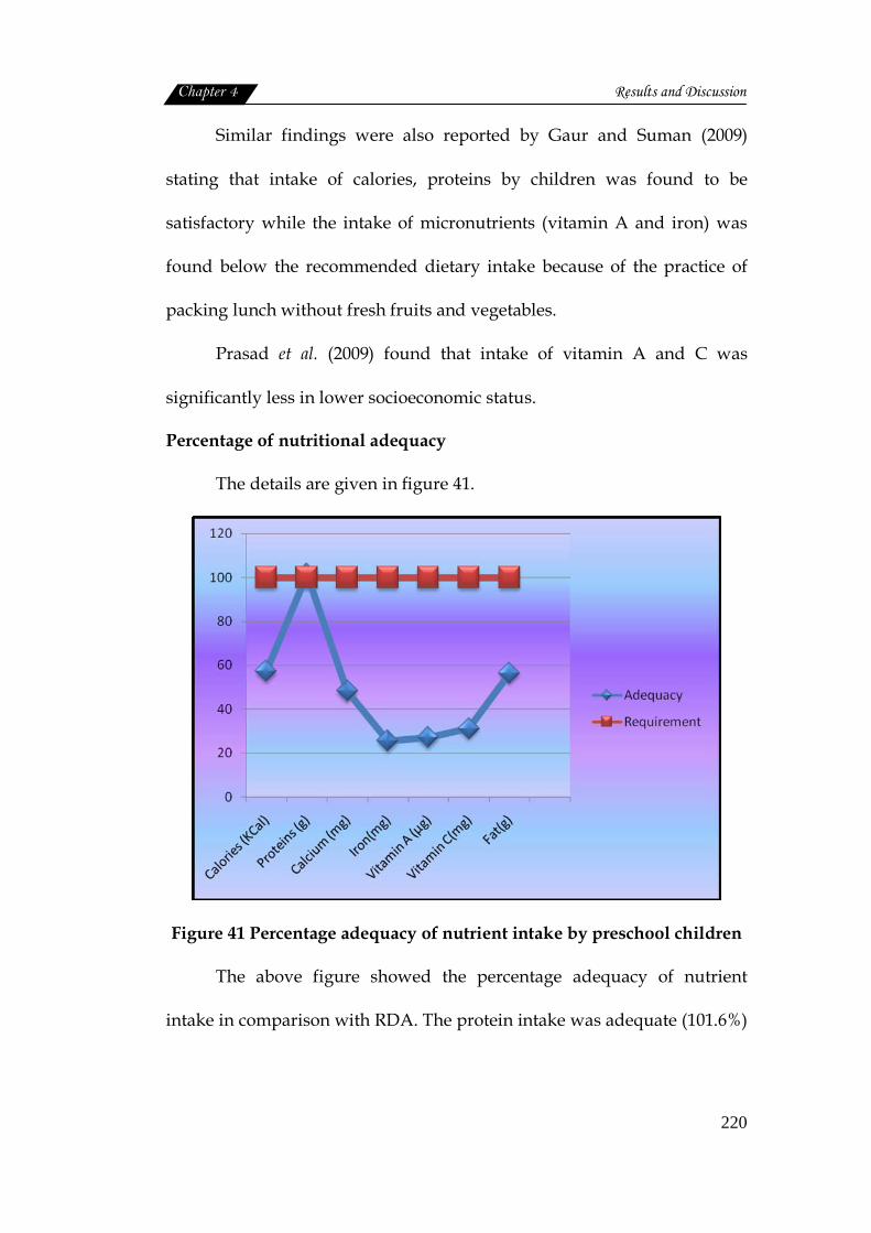
Chapter 4 Results and Discussion
220
Similar findings were also reported by Gaur and Suman (2009)
stating that intake of calories, proteins by children was found to be
satisfactory while the intake of micronutrients (vitamin A and iron) was
found below the recommended dietary intake because of the practice of
packing lunch without fresh fruits and vegetables.
Prasad et al. (2009) found that intake of vitamin A and C was
significantly less in lower socioeconomic status.
Percentage of nutritional adequacy
The details are given in figure 41.
Figure 41 Percentage adequacy of nutrient intake by preschool children
The above figure showed the percentage adequacy of nutrient
intake in comparison with RDA. The protein intake was adequate (101.6%)
Chapter 4 Results and Discussion
221
and that of fat was said to be inadequate as the intake met 56.5 percent of
RDA.
Grave inadequacy was noticed in the case of iron (25.6% of RDA)
and vitamin A (27.23% of RDA). This could lead to serious health
consequences due to micronutrient deficiency.
Intake of energy, calcium and vitamin C estimated to meet 57.3
percent, 48.4 percent and 31.25 percent of the RDA, respectively also
posing acute health problems related to nutritional disorders.
Thus it can be stated that diet consumed by the children of urban
slums, under the study, is totally inadequate in quantity as well as quality.
As NFHS-3 (2006) reported rather than quantity the diet should made
nutrient dense especially micronutrients.
4.3.2 Health status of preschool children
Health of children is invariably bound with their living conditions.
Slum children always succumb to infections which strongly affect their
health status.
4.3.2.1 Nutritional disorders
Nutrients obtained through food have vital effects on physical
growth and development, maintenance of normal body function, physical
activity and health. Nutritious food is important to sustain life (ICMR,
1991). Nutritional disorders occur on deficiency of nutrient intake.
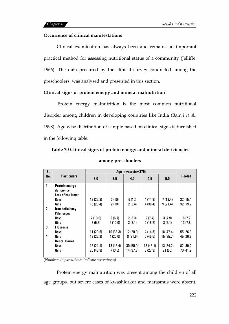
Chapter 4 Results and Discussion
222
Occurrence of clinical manifestations
Clinical examination has always been and remains an important
practical method for assessing nutritional status of a community (Jelliffe,
1966). The data procured by the clinical survey conducted among the
preschoolers, was analysed and presented in this section.
Clinical signs of protein energy and mineral malnutrition
Protein energy malnutrition is the most common nutritional
disorder among children in developing countries like India (Bamji et al.,
1998). Age wise distribution of sample based on clinical signs is furnished
in the following table:
Table 70 Clinical signs of protein energy and mineral deficiencies
among preschoolers
Age in years(n=376) Sl.No. Particulars
3.0 3.5 4.0 4.5 5.0 Pooled
1. 2. 3. 4.
Protein energy deficiency Lack of hair luster Boys Girls Iron deficiency Pale tongue Boys Girls Flourosis Boys Girls Dental Caries Boys Girls
12 (22.3) 15 (26.4)
7 (13.0) 3 (5.3)
11 (20.6) 13 (22.8)
13 (24.1) 25 (43.9)
3 (10) 2 (10)
2 (6.7) 2 (10.0)
10 (33.3) 4 (20.0)
13 (43.4)
7 (3.5)
6 (10) 2 (5.4)
2 (3.3) 3 (8.1)
12 (20.0) 8 (21.6)
30 (50.0) 14 (37.8)
4 (14.8) 4 (36.4)
2 (7.4) 2 (18.2)
4 (14.8) 5 (45.5)
13 (48.1) 3 (27.3)
7 (18.4) 9 (21.4)
3 (7.9) 3 (7.1)
18 (47.4) 15 (35.7)
13 (34.2) 21 (50)
32 (15.4) 32 (19.2)
16 (7.7) 13 (7.8)
55 (26.3) 45 (26.9)
82 (39.2) 70 (41.9)
(Numbers in parentheses indicate percentages)
Protein energy malnutrition was present among the children of all
age groups, but severe cases of kwashiorkor and marasmus were absent.
Chapter 4 Results and Discussion
223
While symptoms like lusterless dry rough hair was found among the boys
(15.4%) as well as girls (19.2%).
Anaemia cases were there in both the groups. The symptoms of
paleness of tongue was observed, while koilonychia was absent.
Irrespective of gender, paleness of tongue was seen among both boys
(7.7%) and girls (7.8%). The incidence of anaemia among 3 year boys and
4.5 year girls.
Flourosis was noticed among the sample involving 26.3 percent of
male and 26.9 percent of female children. Severe form of flourosis as
chalky, pitted and mottled teeth was seen among 5 year old boys (47.4%)
and 4.5 year old girls (45.5%).
Results of dental observation showed that dental hygiene was low
among the children. Dental caries was comparatively more in girls (41.9%)
than in boys (39.2%). Half of the boys in the age group of 4 years and girls
of 5 years had dental caries.
In short, the clinical manifestation of protein energy and iron
deficiencies were more prevalent among the preschoolers in the slum areas
severe form of flourosis was also seen in all age groups irrespective of
gender. Dental caries was the most prominent problem, affecting both boys
(39.2%) and girls (41.9%). Girls in general were more affected than boys.
Age wise prevalence showed that irrespective of gender the upper
age groups (4.5 to 5 years) were more seriously affected than younger
ones. Only exception was the nutritional deficiencies among boys, where 3
year old children were most affected.
Clinical signs of vitamin deficiencies
The details are shown in table 71.

Chapter 4 Results and Discussion
224
Table 71 Clinical signs of vitamin deficiencies among preschoolers
Age (years) Sl.No Particulars 3.0 3.5 4.0 4.5 5.0
Pooled
1.
2.
3.
4.
1.
2.
3.
4.
Vitamin A deficiency Night blindness Boys Girls Conjunctival Xerosis Boys Girls Bitot’s Spot Boys Girls Corneal Xerosis Boys Girls Vitamin B Complex deficiency Angular stomatitis Boys Girls Cheilosis Boys Girls Glossitis Boys Girls Phrynoderma Boys Girls
Nil Nil
5(9.3)
12(21.1)
Nil Nil
Nil
1(1.8)
3(5.6) 4(7.0)
1(1.9)
Nil
4(7.5) 4(7.1)
2(3.0)
Nil
Nil Nil
9(30.0) 1(5.0)
Nil Nil
Nil Nil
Nil Nil
Nil Nil
Nil
2(10.0)
Nil Nil
Nil Nil
8(13.3) 5(13.5)
Nil Nil
1(1.7) 1(2.7)
3(5.0) 1(2.7)
Nil Nil
5(8.3) 2(5.4)
Nil
1(2.7)
Nil Nil
3(11.1) 2(18.2)
Nil Nil
Nil
1(9.1)
1(3.7) 1(9.1)
Nil Nil
1(3.7) 1(9.1)
Nil Nil
1(3.5) Nil
7(18.4) 6(14.3)
1(3.5)
Nil
2(5.3) 3(7.1)
1(2.6) 1(2.4)
Nil Nil
2(5.3)
Nil
Nil Nil
1(0.5) Nil
32(15.3) 26(15.6)
1(0.5)
Nil
3(1.4) 6(3.6)
8(3.82) 7(4.19)
1(0.5)
Nil
12(5.74) 9(5.4)
2(1.0) 1(0.6)
1.
2.
Vitamin C deficiency Spongy and bleeding gums Boys Girls Vitamin D deficiency Knock knee Boys Girls Bow legs Boys Girls
1(1.9) Nil
2(3.7) 1(1.8)
1(1.9)
Nil
Nil Nil
Nil Nil
Nil
1(5.0)
1(1.7) Nil
Nil Nil
Nil Nil
Nil Nil
3(11.1) 1(2.4)
Nil Nil
1(2.6) Nil
Nil Nil
Nil Nil
3(1.5) Nil
5(2.4) 2(1.2)
1(0.5) 1(0.6)
(Numbers in parentheses indicate percentages)
Vitamin A deficiency
Conjunctival xerosis and corneal xerosis, the two manifestations of
vitamin A deficiency were diagnosed among the preschoolers. Among the
sample 15.3 percent of boys and 15.6 percent of girls had conjunctival

Chapter 4 Results and Discussion
225
xerosis followed by corneal xerosis involving 1.4 percent of boys and 3.6
percent of girls. Only one case each of nightblindness and bitot’s spot was
also reported among 5 year old boys. Age wise distribution indicated that
that senior age group (4.5 to 5.0 years) was slightly more affected;
although not much a difference was observed among the different age
groups studied.
In India, Vitamin A Deficiency (VAD) is still a major micronutrient
deficiency lurking beneath childhood morbidity and mortality due to
common illnesses (Bains et al., 2009). Vitamin A deficiency often in
association with protein energy malnutrition principally affects preschool
children. It is estimated that almost 250 million children in developing
countries are at risk (NIPCCD, 2007).
As given by Aneja et al. (2000) signs of Vitamin A deficiency like
bitot’s spot, xeropthalmia and increased morbidity in terms of repeated
bouts of acute respiratory illness, diarrhoeal disease in infants and
children and resultant mortality as well as night blindness in pregnant
women were rampant across most communities.
Ocular signs of vitamin A deficiency were more present among the
children aged 1-5 years. Children of illiterate mothers suffered from
vitamin- A deficiency. Nutrient intake decreases with the increase of
family size, and in children of multipara mothers (Chatterjee et al., 2009).
The prevalence of night blindness, conjunctival xerosis and bitot’s spot
was more and it increased significantly with increase in age, even this was
Chapter 4 Results and Discussion
226
higher among the children of lower socioeconomic communities, in 3-5-year
age group and those children of illiterate mothers (Arlappa et al., 2009). All
the deficiencies were more common amongst male children (Sharma et al.,
2009).
Vitamin A supplementation proved to be definitely effective to
improve the health status of the slum dwellers, about 75 percent of them
suffered from at least one episode of acute respiratory infections
irrespective of the vitamin A supplementation (Kar et al., 2001).
Das et al. (2009) observed the overall prevalence of night blindness,
bitot’s spot and conjunctival xerosis. Higher morbidity rate of diarrhoea,
respiratory disease, measles and skin disease was suggestive of high
prevalence of vitamin A deficiency.
Vitamin B complex deficiency
Angular stomatitis, cheilosis, glossitis and phrynoderma were the
symptoms observed. Of which angular stomatitis and glossitis presented a
slightly more prevalence rate than others. However the overall prevalence
rate was less than 5 percent. Here also girls of all age groups were more
affected than boys.
Vitamin C deficiency
Occurrence of vitamin C deficiency as spongy and bleeding gums
was found only among 1.5 percent of the sample; that too among boys, not
among girls.
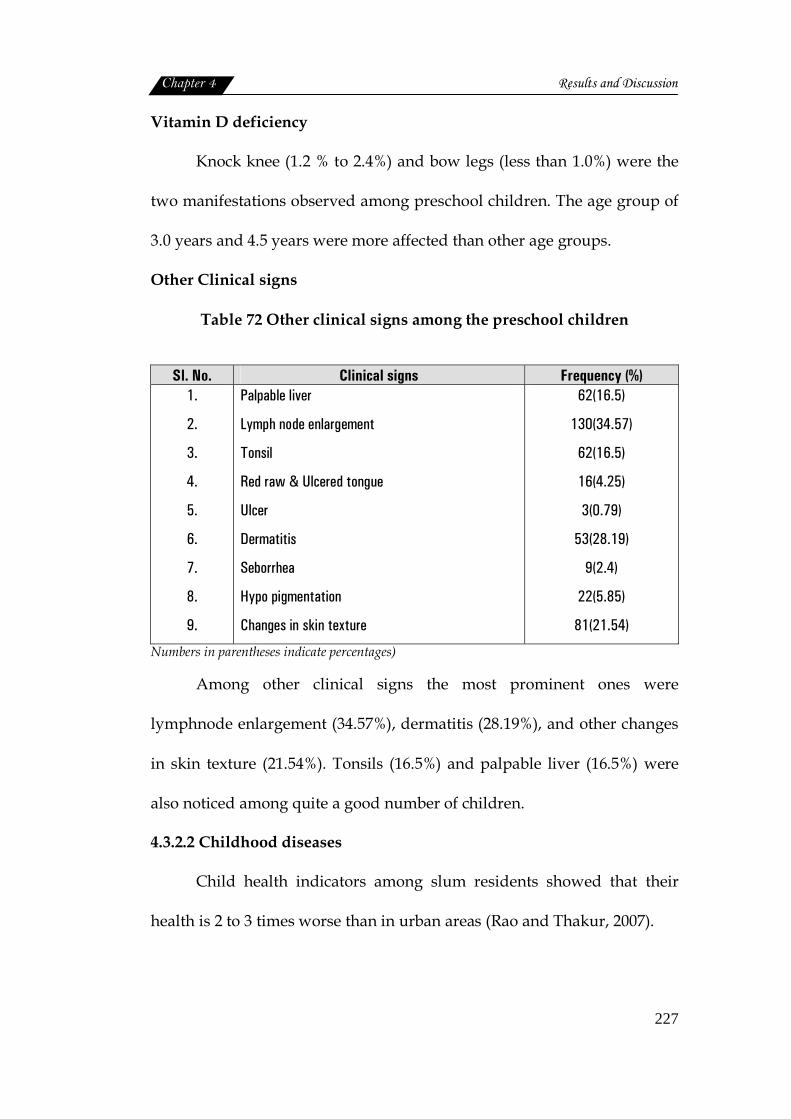
Chapter 4 Results and Discussion
227
Vitamin D deficiency
Knock knee (1.2 % to 2.4%) and bow legs (less than 1.0%) were the
two manifestations observed among preschool children. The age group of
3.0 years and 4.5 years were more affected than other age groups.
Other Clinical signs
Table 72 Other clinical signs among the preschool children
Sl. No. Clinical signs Frequency (%) 1.
2.
3.
4.
5.
6.
7.
8.
9.
Palpable liver
Lymph node enlargement
Tonsil
Red raw & Ulcered tongue
Ulcer
Dermatitis
Seborrhea
Hypo pigmentation
Changes in skin texture
62(16.5)
130(34.57)
62(16.5)
16(4.25)
3(0.79)
53(28.19)
9(2.4)
22(5.85)
81(21.54)
Numbers in parentheses indicate percentages)
Among other clinical signs the most prominent ones were
lymphnode enlargement (34.57%), dermatitis (28.19%), and other changes
in skin texture (21.54%). Tonsils (16.5%) and palpable liver (16.5%) were
also noticed among quite a good number of children.
4.3.2.2 Childhood diseases
Child health indicators among slum residents showed that their
health is 2 to 3 times worse than in urban areas (Rao and Thakur, 2007).
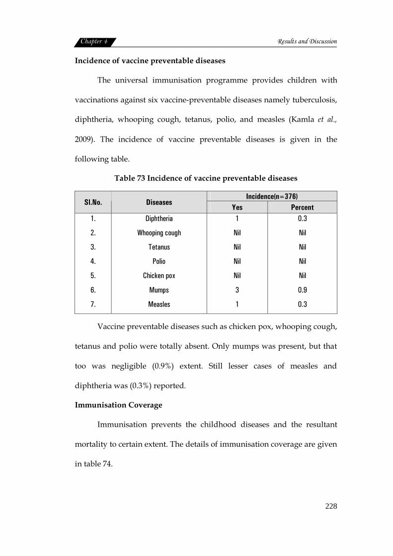
Chapter 4 Results and Discussion
228
Incidence of vaccine preventable diseases
The universal immunisation programme provides children with
vaccinations against six vaccine-preventable diseases namely tuberculosis,
diphtheria, whooping cough, tetanus, polio, and measles (Kamla et al.,
2009). The incidence of vaccine preventable diseases is given in the
following table.
Table 73 Incidence of vaccine preventable diseases
Incidence(n=376) Sl.No. Diseases
Yes Percent 1.
2.
3.
4.
5.
6.
7.
Diphtheria
Whooping cough
Tetanus
Polio
Chicken pox
Mumps
Measles
1
Nil
Nil
Nil
Nil
3
1
0.3
Nil
Nil
Nil
Nil
0.9
0.3
Vaccine preventable diseases such as chicken pox, whooping cough,
tetanus and polio were totally absent. Only mumps was present, but that
too was negligible (0.9%) extent. Still lesser cases of measles and
diphtheria was (0.3%) reported.
Immunisation Coverage
Immunisation prevents the childhood diseases and the resultant
mortality to certain extent. The details of immunisation coverage are given
in table 74.
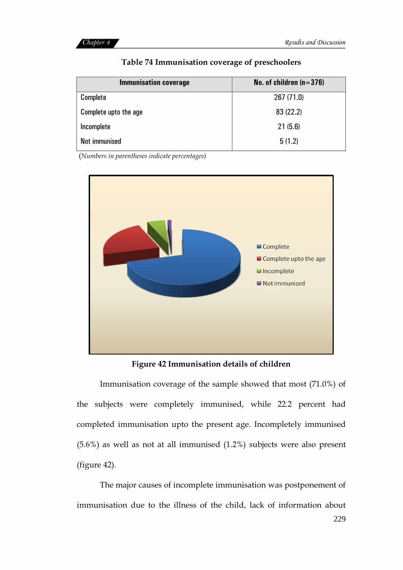
Chapter 4 Results and Discussion
229
Table 74 Immunisation coverage of preschoolers
Immunisation coverage No. of children (n=376)
Complete
Complete upto the age
Incomplete
Not immunised
267 (71.0)
83 (22.2)
21 (5.6)
5 (1.2)
(Numbers in parentheses indicate percentages)
Figure 42 Immunisation details of children
Immunisation coverage of the sample showed that most (71.0%) of
the subjects were completely immunised, while 22.2 percent had
completed immunisation upto the present age. Incompletely immunised
(5.6%) as well as not at all immunised (1.2%) subjects were also present
(figure 42).
The major causes of incomplete immunisation was postponement of
immunisation due to the illness of the child, lack of information about
Chapter 4 Results and Discussion
230
venue and place, schedule and prescribed age of immunisation. Lack of
appropriate information is still the main hurdle for success of primary
immunisation in slum areas (Kar et al., 2001).
Maternal education was found to be positively associated with the
knowledge about immunisation, but was not significantly associated with
actual immunisation practice (Freeman et al., 1992). According to NFHS-3
only 44 per cent of the children are fully immunised (NFHS-3, 2006).
Studies states that the proportion of fully immunised children was
higher in female than males. Slums do have more morbidity as there is no
one being at home to take the child to health services for vaccinations
(Freeman et al., 1992).
Occurrence of other childhood illnesses
The morbidity burden due to respiratory and gastrointestinal illness
is high in a south Indian urban slum, with children ill for approximately
one fifth of infancy, mainly with respiratory and gastro intestinal illness.
The risk factors identified were younger age, male sex, cold/wet season
and household environment (Gladstone et al., 2007). Frequency of
occurrence of childhood diseases is presented in table 75.
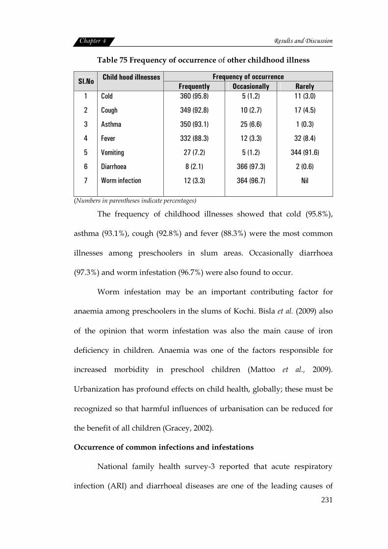
Chapter 4 Results and Discussion
231
Table 75 Frequency of occurrence of other childhood illness
Frequency of occurrence Sl.No Child hood illnesses
Frequently Occasionally Rarely 1
2
3
4
5
6
7
Cold
Cough
Asthma
Fever
Vomiting
Diarrhoea
Worm infection
360 (95.8)
349 (92.8)
350 (93.1)
332 (88.3)
27 (7.2)
8 (2.1)
12 (3.3)
5 (1.2)
10 (2.7)
25 (6.6)
12 (3.3)
5 (1.2)
366 (97.3)
364 (96.7)
11 (3.0)
17 (4.5)
1 (0.3)
32 (8.4)
344 (91.6)
2 (0.6)
Nil
(Numbers in parentheses indicate percentages)
The frequency of childhood illnesses showed that cold (95.8%),
asthma (93.1%), cough (92.8%) and fever (88.3%) were the most common
illnesses among preschoolers in slum areas. Occasionally diarrhoea
(97.3%) and worm infestation (96.7%) were also found to occur.
Worm infestation may be an important contributing factor for
anaemia among preschoolers in the slums of Kochi. Bisla et al. (2009) also
of the opinion that worm infestation was also the main cause of iron
deficiency in children. Anaemia was one of the factors responsible for
increased morbidity in preschool children (Mattoo et al., 2009).
Urbanization has profound effects on child health, globally; these must be
recognized so that harmful influences of urbanisation can be reduced for
the benefit of all children (Gracey, 2002).
Occurrence of common infections and infestations
National family health survey-3 reported that acute respiratory
infection (ARI) and diarrhoeal diseases are one of the leading causes of

Chapter 4 Results and Discussion
232
childhood morbidity and mortality throughout the world. Occurrence of
these illnesses and their statistical significance were found out and
presented in the table below.
Table 76 Slum wise occurrence of common infections and infestations
Sl.No. Slums Respiratory
infection Diarrhoeal diseases
1.
2.
3.
4.
5.
6.
7.
8.
Atlantis
Fort Kochi
Karithala
Pallichal
Puthuvypu
Santhom
Thevara
Vathuruthy
16(47.1)
20(66.7)
6(66.7)
29(56.9)
39(36.4)
12(46.2)
17(35.4)
26(38.2)
26(74.3)
11(36.7)
8(88.9)
36(70.6)
99(92.5)
20(76.9)
34(70.8)
51(72.9)
χ2 value 16.536 43.99
‘p’ value p=0.021* p=0.000**
(Numbers in parentheses indicate percentages) *Significant at 5% level ** Significant at 1 % level
The incidence of respiratory infection among the urban slums
ranged between 34.5 percent to 66.7 percent. This indicated that quite a
good number of preschoolers in urban slums had respiratory infection.
The highest incidence was reported in the Fort Kochi (66.7%) and
Karithala (66.7%) slums. Next in the list was Pallichal (56.9%) followed by
Atlantis (47.1%).
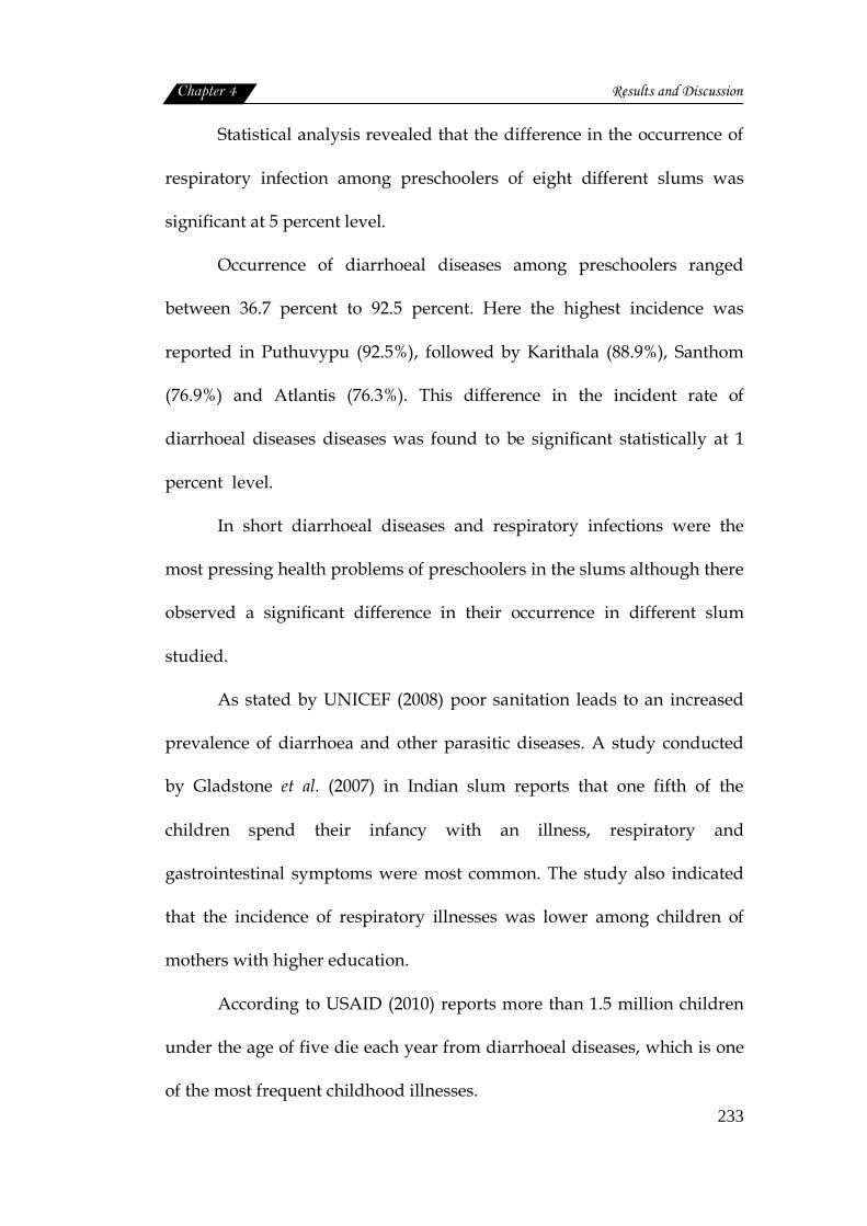
Chapter 4 Results and Discussion
233
Statistical analysis revealed that the difference in the occurrence of
respiratory infection among preschoolers of eight different slums was
significant at 5 percent level.
Occurrence of diarrhoeal diseases among preschoolers ranged
between 36.7 percent to 92.5 percent. Here the highest incidence was
reported in Puthuvypu (92.5%), followed by Karithala (88.9%), Santhom
(76.9%) and Atlantis (76.3%). This difference in the incident rate of
diarrhoeal diseases diseases was found to be significant statistically at 1
percent level.
In short diarrhoeal diseases and respiratory infections were the
most pressing health problems of preschoolers in the slums although there
observed a significant difference in their occurrence in different slum
studied.
As stated by UNICEF (2008) poor sanitation leads to an increased
prevalence of diarrhoea and other parasitic diseases. A study conducted
by Gladstone et al. (2007) in Indian slum reports that one fifth of the
children spend their infancy with an illness, respiratory and
gastrointestinal symptoms were most common. The study also indicated
that the incidence of respiratory illnesses was lower among children of
mothers with higher education.
According to USAID (2010) reports more than 1.5 million children
under the age of five die each year from diarrhoeal diseases, which is one
of the most frequent childhood illnesses.
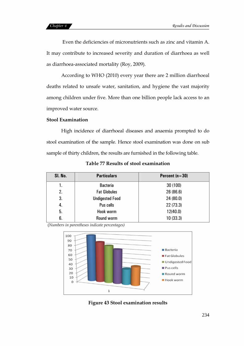
Chapter 4 Results and Discussion
234
Even the deficiencies of micronutrients such as zinc and vitamin A.
It may contribute to increased severity and duration of diarrhoea as well
as diarrhoea-associated mortality (Roy, 2009).
According to WHO (2010) every year there are 2 million diarrhoeal
deaths related to unsafe water, sanitation, and hygiene the vast majority
among children under five. More than one billion people lack access to an
improved water source.
Stool Examination
High incidence of diarrhoeal diseases and anaemia prompted to do
stool examination of the sample. Hence stool examination was done on sub
sample of thirty children, the results are furnished in the following table.
Table 77 Results of stool examination
Sl. No. Particulars Percent (n=30)
1. 2. 3. 4. 5. 6.
Bacteria Fat Globules
Undigested Food Pus cells
Hook worm Round worm
30 (100) 26 (86.6) 24 (80.0) 22 (73.3) 12(40.0) 10 (33.3)
(Numbers in parentheses indicate percentages)
Figure 43 Stool examination results
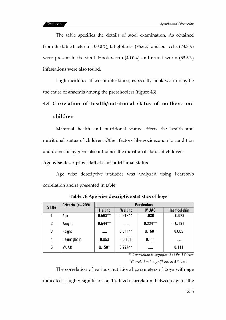
Chapter 4 Results and Discussion
235
The table specifies the details of stool examination. As obtained
from the table bacteria (100.0%), fat globules (86.6%) and pus cells (73.3%)
were present in the stool. Hook worm (40.0%) and round worm (33.3%)
infestations were also found.
High incidence of worm infestation, especially hook worm may be
the cause of anaemia among the preschoolers (figure 43).
4.4 Correlation of health/nutritional status of mothers and
children
Maternal health and nutritional status effects the health and
nutritional status of children. Other factors like socioeconomic condition
and domestic hygiene also influence the nutritional status of children.
Age wise descriptive statistics of nutritional status
Age wise descriptive statistics was analyzed using Pearson’s
correlation and is presented in table.
Table 78 Age wise descriptive statistics of boys
Particulars Sl.No Criteria (n=209) Height Weight MUAC Haemoglobin
1
2
3
4
5
Age
Weight
Height
Haemoglobin
MUAC
0.563**
0.544**
…..
0.053
0.150*
0.513**
…..
0.544**
- 0.131
0.224**
.036
0.224**
0.150*
0.111
…..
- 0.028
- 0.131
0.053
…..
0.111
** Correlation is significant at the 1%level
*Correlation is significant at 5% level
The correlation of various nutritional parameters of boys with age
indicated a highly significant (at 1% level) correlation between age of the
Chapter 4 Results and Discussion
236
boys and their heights and weights. This indicated that height and weight
of the boys significantly correlated with their age. In the case of MUAC ,
an increase was seen with age but not to any significant extent. Whereas,
haemoglobin status showed a negative correlation with age of the children
(Boys) which was not statistically significant.
The weight of the boys showed a highly significant (at 1 % level)
positive correlation with height of boys and MUAC; and insignificant
negative correlation was observed with haemoglobin status: i.e., as the
weight increase height and MUAC of boys also increased significantly (at
1% level) but haemoglobin status decreased though not to any significant
level.
Height of boys also found to increase with body weight (significant
at 1% level) and MUAC (significant at 5 % level). Haemoglobin status
failed to show any significant correlation with height, weight and MUAC.
At the same time MUAC had a significant correlation with height of boys
(P<0.01) and weight of boys (P< 0.01).
Age wise descriptive statistics of girls
Pearson’s correlation was applied to find out various factors used in
the assessment of nutritional status and their correlation. The details are
presented in the following table.
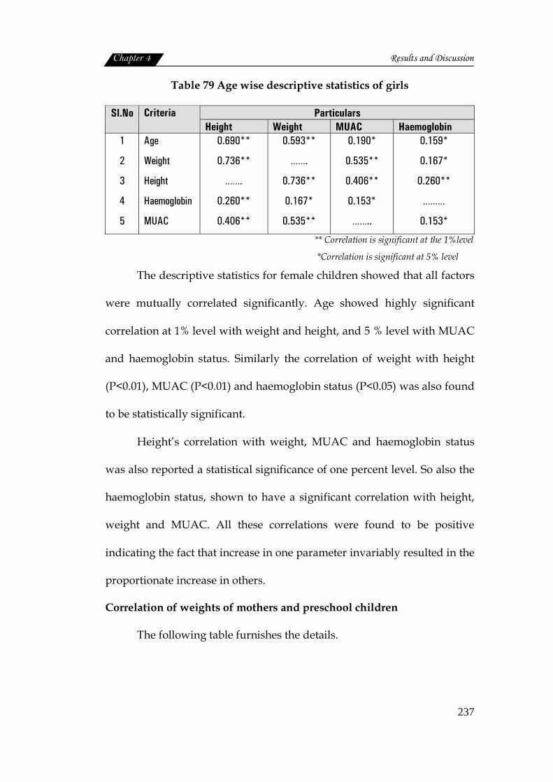
Chapter 4 Results and Discussion
237
Table 79 Age wise descriptive statistics of girls
Particulars Sl.No Criteria Height Weight MUAC Haemoglobin
1
2
3
4
5
Age
Weight
Height
Haemoglobin
MUAC
0.690**
0.736**
…….
0.260**
0.406**
0.593**
…….
0.736**
0.167*
0.535**
0.190*
0.535**
0.406**
0.153*
……..
0.159*
0.167*
0.260**
………
0.153*
** Correlation is significant at the 1%level
*Correlation is significant at 5% level
The descriptive statistics for female children showed that all factors
were mutually correlated significantly. Age showed highly significant
correlation at 1% level with weight and height, and 5 % level with MUAC
and haemoglobin status. Similarly the correlation of weight with height
(P<0.01), MUAC (P<0.01) and haemoglobin status (P<0.05) was also found
to be statistically significant.
Height’s correlation with weight, MUAC and haemoglobin status
was also reported a statistical significance of one percent level. So also the
haemoglobin status, shown to have a significant correlation with height,
weight and MUAC. All these correlations were found to be positive
indicating the fact that increase in one parameter invariably resulted in the
proportionate increase in others.
Correlation of weights of mothers and preschool children
The following table furnishes the details.

Chapter 4 Results and Discussion
238
Table 80 Correlation of weights of mothers and preschool children
Sl.No Particulars Mean Weight (Kg)
Standard deviation
Corelation coefficient
p value
1
2
Weight of Mother
Weight of child
51.23
13.45
±9.95
±2.57 0.137 0.008*
* significant at 5 % level
The weight of the mothers and that of their preschool children had a
positive correlation which was statistically significant at 5 percent level.
This indicated that mothers with normal body weight give birth to babies
with normal birth weight (>2.5 Kg). Low birth weight babies were born to
undernourished mothers whose baby weight was subnormal. Maternal
and child health indicators among slum dwellers show that their health is
2 to 3 times worse than in urban areas (Rao and Thakur, 2007).
Correlation of haemoglobin status of mothers and preschool children
The following table analyzes the correlation between the
haemoglobin status mother and child.
Table 81 Correlation of haemoglobin status of mothers and preschool
children
Sl.No Particulars Mean
Haemoglobin value (g/dl)
Standard Deviation
Correlation coefficient
‘p’ value
1
2
Mother
Children
11.03
10.17
±1.15
±1.15 0.073 0.155 NS
NS-Not Significant
The table revealed that haemoglobin distribution of mother and child
are positively correlated but this was statistically not significant. The mean
haemoglobin level of mother was 11.03 and of children was 10.17. Nutritional
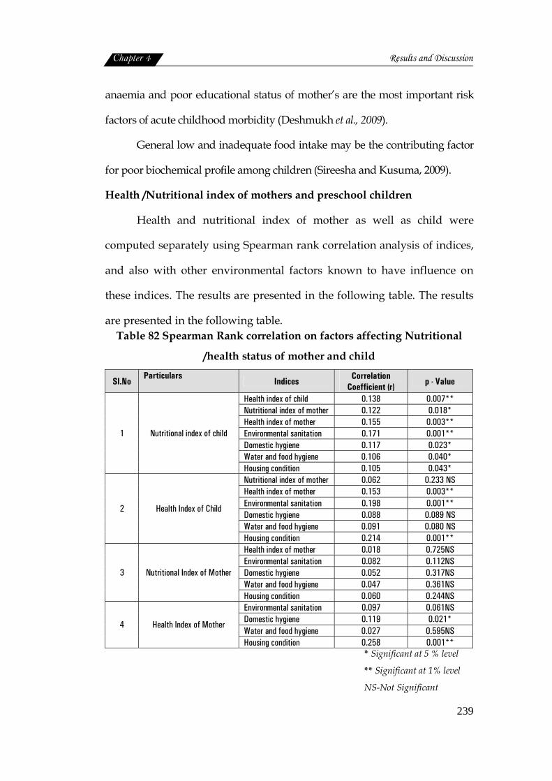
Chapter 4 Results and Discussion
239
anaemia and poor educational status of mother’s are the most important risk
factors of acute childhood morbidity (Deshmukh et al., 2009).
General low and inadequate food intake may be the contributing factor
for poor biochemical profile among children (Sireesha and Kusuma, 2009).
Health /Nutritional index of mothers and preschool children
Health and nutritional index of mother as well as child were
computed separately using Spearman rank correlation analysis of indices,
and also with other environmental factors known to have influence on
these indices. The results are presented in the following table. The results
are presented in the following table. Table 82 Spearman Rank correlation on factors affecting Nutritional
/health status of mother and child
Sl.No Particulars
Indices Correlation Coefficient (r) p - Value
Health index of child 0.138 0.007** Nutritional index of mother 0.122 0.018* Health index of mother 0.155 0.003** Environmental sanitation 0.171 0.001** Domestic hygiene 0.117 0.023* Water and food hygiene 0.106 0.040*
1 Nutritional index of child
Housing condition 0.105 0.043* Nutritional index of mother 0.062 0.233 NS Health index of mother 0.153 0.003** Environmental sanitation 0.198 0.001** Domestic hygiene 0.088 0.089 NS Water and food hygiene 0.091 0.080 NS
2 Health Index of Child
Housing condition 0.214 0.001** Health index of mother 0.018 0.725NS Environmental sanitation 0.082 0.112NS Domestic hygiene 0.052 0.317NS Water and food hygiene 0.047 0.361NS
3 Nutritional Index of Mother
Housing condition 0.060 0.244NS Environmental sanitation 0.097 0.061NS Domestic hygiene 0.119 0.021* Water and food hygiene 0.027 0.595NS
4 Health Index of Mother
Housing condition 0.258 0.001** * Significant at 5 % level
** Significant at 1% level
NS-Not Significant
Chapter 4 Results and Discussion
240
The above table gives a detailed picture of the health and nutritional
index of mothers and preschool children as well as related factors
influencing them.
Nutritional and Health index of children
From the table it is obvious that nutritional index of children has a
direct correlation with all the factors studied. The factors like health index
of child (P<0.01), health index of mother (P<0.01) and environmental
sanitation (P<0.01) showed a highly significant correlation with nutritional
index of child. Whereas statistical significance at 5 percent level was
reported by other parameters like nutritional index of mother (P<0.05)
housing condition (P<0.05) and hygienic practices like domestic (P<0.05)
and water food hygiene (P<0.05).
At the same time health index of the children did not show any
significant correlation with nutrition index of mother and hygienic
practices of the family. Whereas health index of the mother (P<0.01)
housing condition (P<0.01) and environmental sanitation (P<0.01) all had
highly significant correlation with the health index of the children. Poor
housing condition and the resultant insanitary living environment in the
slums are conducive for the spread of infectious diseases. As stated by
Chandramouli (2003) living conditions have a direct impact on public
health.
Chapter 4 Results and Discussion
241
Nutritional and health index of mothers
Nutritional index of mothers found to have no significant
correlation with any of the parameters studied. This is to mean that health
index of mothers, housing conditions and environmental and domestic,
water and food hygiene none of these could influence the nutritional index
of mothers.
But health index of the mothers was significantly correlated with
housing conditions (P<0.01) and domestic hygiene (P<0.05)
All these findings direct to say that more than the nutritional
deprivation; housing conditions and poor hygiene and insanitary
environment in slums, are more decisive in the health and nutritional well
being of mothers and children. The environmental sanitation playing an
important role on the nutritional status has already been reported by
UNICEF (2009).
Further personal and domestic hygienic practices according to Nath
(2003) cannot be improved without improving basic amenities, such as
water supply, waste water disposal, solid waste management and the
problems of human settlements.
UNICEF (2009) stated that a child’s future nutrition status is
affected before conception and is greatly dependent on the mother’s
nutrition status prior to and during pregnancy. A chronically
undernourished woman will give birth to a baby who is likely to be
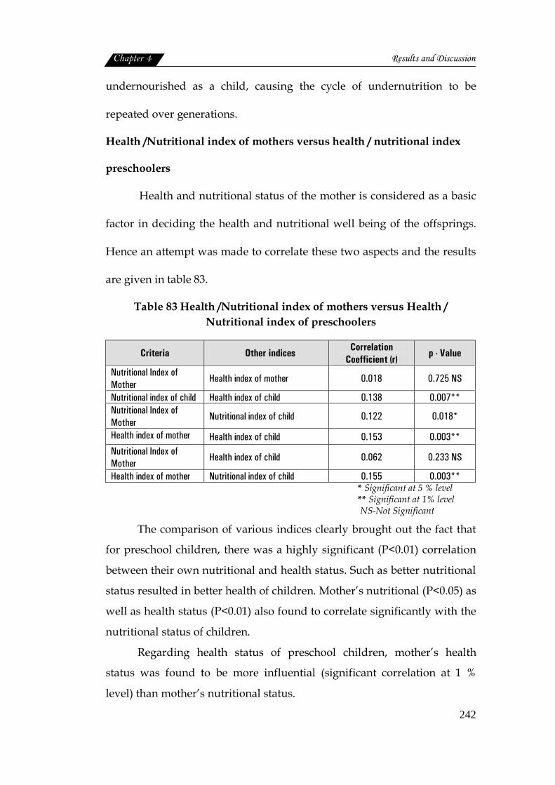
Chapter 4 Results and Discussion
242
undernourished as a child, causing the cycle of undernutrition to be
repeated over generations.
Health /Nutritional index of mothers versus health / nutritional index
preschoolers
Health and nutritional status of the mother is considered as a basic
factor in deciding the health and nutritional well being of the offsprings.
Hence an attempt was made to correlate these two aspects and the results
are given in table 83.
Table 83 Health /Nutritional index of mothers versus Health / Nutritional index of preschoolers
Criteria Other indices Correlation Coefficient (r)
p - Value
Nutritional Index of Mother
Health index of mother 0.018 0.725 NS
Nutritional index of child Health index of child 0.138 0.007** Nutritional Index of Mother
Nutritional index of child 0.122 0.018*
Health index of mother Health index of child 0.153 0.003** Nutritional Index of Mother
Health index of child 0.062 0.233 NS
Health index of mother Nutritional index of child 0.155 0.003** * Significant at 5 % level ** Significant at 1% level NS-Not Significant
The comparison of various indices clearly brought out the fact that
for preschool children, there was a highly significant (P<0.01) correlation
between their own nutritional and health status. Such as better nutritional
status resulted in better health of children. Mother’s nutritional (P<0.05) as
well as health status (P<0.01) also found to correlate significantly with the
nutritional status of children.
Regarding health status of preschool children, mother’s health
status was found to be more influential (significant correlation at 1 %
level) than mother’s nutritional status.
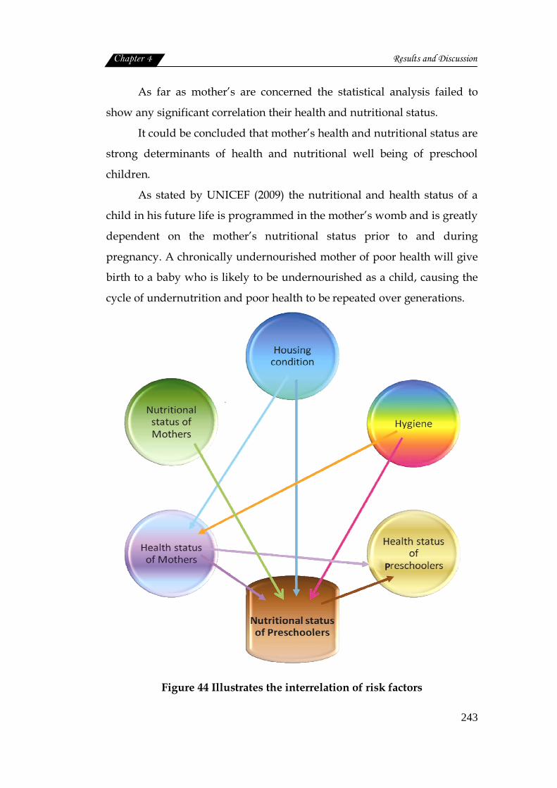
Chapter 4 Results and Discussion
243
As far as mother’s are concerned the statistical analysis failed to
show any significant correlation their health and nutritional status.
It could be concluded that mother’s health and nutritional status are
strong determinants of health and nutritional well being of preschool
children.
As stated by UNICEF (2009) the nutritional and health status of a
child in his future life is programmed in the mother’s womb and is greatly
dependent on the mother’s nutritional status prior to and during
pregnancy. A chronically undernourished mother of poor health will give
birth to a baby who is likely to be undernourished as a child, causing the
cycle of undernutrition and poor health to be repeated over generations.
Figure 44 Illustrates the interrelation of risk factors