RESOURCE USE EFFICIENCY IN VEGETABLE PRODUCTION: THE CASE OF SMALLHOLDER FARMERS IN THE KUMASI METROPOLIS. BY

ADAMS ABDULAI THIS THESIS IS SUBMITTEDN TO THE UNIVERSITY OF SCIENCE AND TECHNOLOGY, IN PARTIAL FULFILLMENT OF THE REQUIREMENTS FOR THE AWARD OF MASTER OF SCIENCE DEGREE IN AGRICULTURAL ECONOMICS.

DEPARTMENT OF AGRICULTURAL ECONOMICS, AGRIBUSINESS &EXTENSION.

COLLEGE OF AGRICULTURE & RENEWABLE NATURAL RESOURCES.

AUGUST, 2006

i

DECLARATION I, ADAMS ABDULAI, author of this thesis titled ‘Resource use efficiency of Vegetable

production: the case of smallholder farmers in the Kumasi Methropolis’do hereby declare

that, apart from the references of other peoples work, which has been duly acknowledged,

the research work presented in this thesis was done entirely by me at the Department of

Agricultural Economics, Agribusiness & Extension, University of Science and

Technology, Kumasi from August 2005 to August 2006.

I do further declare that, this work has neither been presented in whole nor in part for any

degree at this University or elsewhere.

.……………………………………

Adams Abdulai (STUDENT) ……………………………. ……………………………………

Dr.S.C Fialor Dr.J.A Bakang (Major Supervisor) (Co-Supervisor)

ii

DEDICATION

This work is dedicated to all my family and fiends, especially my mother, Awusara

Adams whose priceless sacrifice and encouragement has made it possible for me to

materialize this dream. God bless us all.

iii

ACKNOWLEDGEMENT

I wish to express my sincere gratitude to the Almighty God for bringing me this far. I am

very grateful to all persons who offered invaluable contributions and suggestions as to

how this thesis might be organized and made useful. Dear to my heart are my supervisors

Dr S.C Fialor and Dr.J.A Bakang who not only encouraged me but also challenged me

with very useful comments to work harder throughout this academic programme.This

dissertation could not have been written without them. I say thank you and God richly

bless you.

I am very grateful to the Challenge programme for food and water for providing financial

support for Data collection through the Department of Agricultural economics,

Agribusiness & Extension. I wish to thank Dr.Ohene Yankyira and all Lecturers of the

Department of Agricultural economics, Agribusiness & Extension for their constructive

criticisms and useful suggestions made during the course of writing this dissertation.

Special mention must be made of the fatherly care of the headmaster of Wa Islamic

Senior secondary school, Mr.Alhassan Suleman for his encouragement, Tolerance and

support shown during the course of pursuing this programme.

I wish to express my sincere gratitude to my course mates,Awusi Ebenezer

Mahama,Fiatuse Vivian,Oteng Fredrick Mensah,Gashon,Ismail Abass, and Slim for their

friendly love, contributions and support .I am also very grateful to Robert Aidoo,Haruna

Issahaku,Richard Bankalle,and Raymond Ayine .I appreciate the support from you all.

iv

ABSTRACT

This study attempts to find out the current levels of efficiency of some selected vegetable

farmers in the Kumasi metropolis. Both Technical and allocative efficiencies were

analysed and compared.Further, the effects of some socio-economic variables on

efficiency were estimated and compared. The productivity of land and labour in the

production process as well the perception of farmers on waste water use were also

analysed.

Technical efficiency estimates were obtained using the Stochastic Efficiency Frontier

model whiles the allocative efficiency estimates were obtained using the marginal

product approach. Productivity of land and labour were estimated using partial

productivity measures, the ratio of output to an individual input or input class.

Descriptive statistics were used in determine the perception of farmers on water use.

The study found that inefficiency in the vegetable production system exists. The mean

technical efficiency of the pooled sample is 66.67%.Efficiency level varies across all

production units ranging from 12.9% to 95.02%. There is no significant difference in

technical efficiency estimates between production units at 5% level of significance.

Over 80% of vegetable producers covered by the study do not owe land permanently to

undertake any meaningful production. The implication is that, investments made in

developing the land is minimal or non-existent, permanent farm structures cannot be

erected and the future of the vegetable industry is uncertain though it proof profitable to

most farmers.

v

The allocative efficiency indices for land and labour obtained from the study are 0.4556

and 0.4651 respectively. The implication is that both factors of production are

overutilised in the production process. The effect of labour on agricultural output is

therefore insignificant. This is consistent with the proposition that the use of labour in the

agricultural sector is inefficient.

The productivity of land, labour and water were estimated to be ¢91,525,684 per hectare,

¢72,119 per man days and ¢654,754 per cubic meter respectively. Crop water use

efficiency as well as field water use efficiency was also estimated to be 1061.71kg/m3

and 203.08kg/m3 respectively.

The study revealed that majority of farmers is aware of the health implications associated

with the use of untreated waste water for irrigation. . About 91.5% of farmers hold the

view that the quality of water being used for irrigation is good and do not pose any threat

to the lives of consumers. Water quality is of little priority concern to farmers. What

matters most to them is regular supply of water all year round since most of them do not

pay for it.

vi

TABLE OF CONTENT

Page Declaration……………………………………………………………………………….i Dedication………………………………………………………………………………..ii Acknowledgement……………………………………………………………………….iii Abstract…………………………………………………………………………………..iv Table of Content………………………………………………………………………….vi List of Tables……………………………………………………………………………..x

List of Figures…………………………………………………………………………….xi

List of Acronyms………………………………………………………………………...xii CHAPTER ONE - INTRODUCTION 1.0 Introduction……………………………………………………………………………1 1.1Background…………………………………………………………………….............1 1.2Statement of the Problem………………………………………………………………4 1.3 Objectives of the Study………………………………………………………………..6 1.4 Justification of the study………………………………………………………………7 1.5 hypothesis of the Study………………………………………………………………..9 1.6 Organization of the study……………………………………………………………..9 CHAPTER TWO – REVIEW OF RELATED LITERATURE 2.0 Introduction…………………………………………………………………………..10 2.1Socio-Economic importance of vegetables…………………………………………...12 2.1The concept of Productivity, economic price and technical efficiency………………14 2.1.1The concept of efficiency…………………………………………………………...18

vii

2.1.2 The concept of productivity……………………………………………………….19 2.2 Factors Influencing efficiency………………………………………………………24 2.3 Resources in vegetable production………………………………………………….24 2.3.1 Land……………………………………………………………………………….25 2.3.2 Labour……………………………………………………………………………..26 2.3.3 Capital……………………………………………………………………………..26 2.3.4 Water……………………………………………………………………………....30 2.3.5 Poultry manure………………………………………………………………….…31 2.4 Marketing of vegetables……………………………………………………………..31 2.4.1 Storage and grading………………………………………………………………..33 2.4.1.2 Marketing information…………………………………………………………..34 2.4.1.3 Pricing…………………………………………………………………………...34 2.4.1.4 Demand………………………………………………………………………….35 2.5 Methodological issues……………………………………………………………….35 2.6 Deterministic Versus stochastic specification……………………………………….37 2.7 Empirical studies: Estimation of efficiency & Inefficiency equations……………...41 2.8 Causes of Inefficiency………………………………………………………………42 CHAPTER THREE - METHODOLOGY 3.0 Introduction………………………………………………………………………….44 3.1The study area………………………………………………………………...............44 3.2 Source of data, population and sampling……………………………………….........45 3.3Data collection techniques……………………………………………………………46 3.4 Theoretical framework……………………………………………………............ …46

viii

3.4.1 Theory of productive efficiency…………………………………………................47 3.4.2 Stochastic production frontier Analysis and measurement of efficiency………….51 3.4.3 Empirical estimation of technical efficiency………………………………………52 3.4.4 Socio-economic model…………………………………………………………….54 3.4.5 Empirical estimation of allocative efficiency……………………………………..55 3.5 Hypothesis testing…………………………………………………………………..57 3.6 Estimation of stochastic frontier and technical efficiency functions……………….58 3.7 Definition of Variables……………………………………………………………..58 3.7.1 List of variables …………………………………………………………………..59 3.7.2 Inputs……………………………………………………………………………..59 3.7.3 Determinants of efficiency………………………………………………………..60

CHAPTER FOUR – RESULTS AND DISCUSSION

4.0 Introduction………………………………………………………………………….61

4.1.1Estimates of the production frontier function……………………………………..61

4.1.2 Technical Efficiency estimates……………………………………………………64

4.1.3 Hypothesis Testing………………………………………………………………..65

4.2 Allocative efficiency estimates………………………………………………….....67

4.3 Determinants of Efficiency………………………………………………………….69

4.4 Productivity of land and labour……………………………………………………..72

4.5 Resources in vegetable production………………………………………………….76

4.5.1 Land……………………………………………………………………………….76

4.5.2 Water……………………………………………………………………………...77

4.5.2.1 Sources of water used in irrigation……………………………………………...77

ix

4.5.2.2 Farmers Reasons for not drinking the water used for irrigation………………...78

4.6 Perception of water use……………………………………………………………...79

4.7 Marketing of Vegetables…………………………………………………………….81

4.7.1 Problems of marketing Lettuce and cabbage………………………………………81

CHAPTER FIVE – SUMMARY, CONCLUSIONS AND RECOMMENDATIONS

5.1 Summary……………………………………………………………………………..84

5.2 Conclusions…………………………………………………………………………..88

5.3 Recommendations……………………………………………………………………89

Bibliography……………………………………………………………………..91

Appendices……………………………………………………………………….97

x

LIST OF TABLES

Table 1: Estimates of Vegetable production using Cobb-Douglas frontier function…….62

Table 2: ML estimates of pooled sample using Cobb-Douglas frontier function………..63

Table 3: Frequency distribution of Technical efficiency estimates……………………...64

Table 4: Test of Hypothesis on Technical efficiency…………………………………....66

Table 5: Test of significance differences in efficiency between production units……....67

Table 6: Allocative efficiency estimates…………………………………………………69

Table 7: Determinants of efficiency……………………………………………………..70

Table 8: Productivity estimates………………………………………………………......74

Table 9: Sources of water used in irrigation……………………………………………..78

Table 10: Farmers reasons for not drinking water used for irrigation…………………...79

Table 11: Problems of marketing Vegetables…………………………………………....82

xi

LIST OF FIGURES

Figure 1: Map of Urban Vegetable sites in Kumasi……………………………………45

Figure 2: Land tenure / ownership……………………………………………………..76

Figure 3: Perception of water quality…………………………………………………..80

LIST OF ACRONYMES

ML: Maximum Likelihood

xii

OLS: Ordinary Least Squares

MFC: Marginal Factor Cost

SPF: Stochastic Production frontier

COLS: Corrected Ordinary Least Square

ANOVA: Analysis of Variance

KMA: Kumasi Metropolitan Assembly

IWMI: International Water Management Institute

DEA: Data Envelopment Analysis

iid: Identically and independently distributed

MPP: Marginal Physical Product

MVP: Marginal Value Product

xiii

1

CHAPTER ONE

INTRODUCTION

1.1Background

Agriculture is the main stay of most African countries. Ghana’s economy for the instance

depends largely on its agricultural production. Over the past decade the share of the domestic

agriculture in real aggregate national output averaged about 53% annually, Agriculture

contributes the food needs of the country. The share of the domestic output and consumption of

maize, sorghum and rice for instance were 61.1, 75.8, and 47.8 percent per annum respectively

during the past decade (Haizel, 1994).

It was further observed that, agriculture was by far the chief employer in Ghana,

representing 66% of the total labour force, and 80% of the working population depended

directly or indirectly on agriculture for their livelihood. The agricultural sector is the

largest in terms of contribution to GDP (49%), export (70%), and employment (66%),

according to the 1989 figures (Asuming-Brempong, 1991).A distortion of the agricultural

sector will therefore have an adverse effect on the entire economy. For instance, Killict

(1978) and Bequele (1983) were of the view that the retrogression of the Ghanaian

economy in the 1970’s was largely attributed to the decline in the agricultural sector

during that period.

Vegetables may be described as those plants, which are consumed in relatively small

quantities as a side dish with the staple food. The term ‘vegetable’ can also be used to

designate the tender edible shoots, leaves, fruits and roots of plants that are eaten whole

2

or part raw or cooked as a supplement to starchy foods and meets (Williams et al, 1991).

Vegetables can be distinguished from field crops by the fact that, vegetables are

harvested when the plant is fresh and high in moisture while the fields crops are

harvested at the mature stage for their grains seeds, roots fibre etc.In human nutrition,

vegetables are an essential protective food containing vitamins and minerals. Any

balanced diet should include vegetables and fruits for this reason. The proportion of

vegetables required in a balanced diet per capita per meal is of the order of 45% of the

total volume of the food. Vegetables supply considerable quantities of vitamins A, B, C,

D, E and K.According to Agusiobo (1984) vitamin A maintains health of the respiratory

and the eye tissue; vitamin B is essential for development of the nervous system; vitamin

C maintains health of blood cells and tissues; vitamin D maintains health of bones and

teeth; vitamin E maintains heath of the reproductive system; and vitamin K is essential

for blood clotting. Iron, which is particularly plentiful in green vegetables, is part of

haemoglobin which is found in the blood. The high fibre content of vegetables is

essential to maintain the health of the bowels, and a diet which is low in fruit and

vegetables frequently results in constipation.Tindall (1983) observed that the leaves of

lettuce and cabbage combined supply 184g water; 2.9g protein, 8g carbohydrates, 1.5mg

Iron, 49mg phosphorus, 55mg Ascorbic acid, 1.1mg Niacin, 0.8mg Riboflavin, and

0.2mg Thiamin nutrients per 100g of edible portion.

In Africa, three major classes of vegetables are consumed. These include those that are

gathered from the wild such as baobab leaves; those indigenous vegetables which are

often gathered but are also cultivated such as amaranthus; and imported vegetable species

which are cultivated (Rice et al, 1987). The exotic vegetables under study (Lettuce,

3

cabbage, and carrots) fall under the third category. These vegetables are cultivated in the

country and are highly patronized by most people especially the middle and high-income

classes in the urban areas.

About 800 million people are engaged in urban and peri- urban agriculture worldwide

and contribute about 30% to the worlds food supply (UNDP, 1996). This is increasingly

becoming a common expression of most urban areas in developing countries and is seen

as an important means of attaining balanced diets and urban food security. In several

West African countries, between 50 and 90% of the vegetable consumed are produced

within or close to the city (Cofie et al, 2003).

Vegetable and vegetable products especially processed forms imported form an essential

part of the food in most African countries. This involves the use of limited hard-earned

foreign exchange available. Vegetables are important items in the human diet because

they supply nutrients such as vitamins and minerals and the bulk of roughage the body

needs and which are often lacking in most traditional staple foods.

In recent times there has been a tremendous interest and increase in vegetable crop

production in West Africa. This is because of the urgent need to stop the importation of

vegetables and vegetable products to help conserve foreign exchange and feed the

increasing number of processing factories while exporting the rest to earn more foreign

exchange (Norman, 1992). Vegetables and fruit crops add about add about 3% to the

GDP of the economy of Ghana (PPMED, 1991). Even though the contribution to the

4

GDP is very small, its importance cannot be overlooked because without it a diet is not

balanced.

In Ghana, backyards are mainly used to cultivate vegetable crops in the urban peri-urban

areas by men while marketing of the produce is predominantly in women domain. It also

has significant contributions to livelihoods and food security. According to Danso et al

(2003), urban farmers grow 90% of the main vegetables eaten in the city of Kumasi.This

is done on virtually every open space more close to water sources of almost all major

cities and urban centers in the west African sub-region (Danso et al, 2003).

The efficiency of vegetable production is very crucial in determining the returns on

investment. Quite often the introduction of new technology has been used as a standard

for distinguishing between a modern system and a traditional system (Schultz, 1964), and

for improving the efficiency of the production system. However in the developing world,

some new technologies have been barely successful in improving productive efficiency.

This has often been blamed on the lack of ability and /or willingness on the part of

producers to adjust input levels because of their familiarity with traditional agricultural

systems and or the presence of institutional constraints (Ghatak and Ingerset, 1983).

1.2 Problem statement

In Ghana urban agriculture has not received the appropriate public and institutional

support despite its significant contributions to urban food security, poverty alleviation,

women empowerment and improved human nutrition through the provision of balanced

diets. Ghana has a high potential and positive comparative advantage for vegetable

5

production. Considerable evidence suggests that serious bottlenecks exist in the

functioning of the production system in Ghana.

Anecdotal evidence and inquiry suggest that, a number of factors are responsible for the

low vegetable production at the household level. A question then arises as to how

efficient farmers are using or combining the available scarce resources at their disposal to

produce the maximum desired output.

The food production system in Ghana is largely unorganized and inefficient. Post-harvest

problems from the farm to the retail level results in high losses, high costs of foodstuffs,

and disincentive and discouragement to producers, marketers and consumers. However

urban population growth is fuelling the demand for a timely supply of fresh vegetables

and much of this demand is satisfied through peri-urban production (Jansen et al, 1996).

The problems are acute for dry season vegetable crops. There has however, been little

research to ascertain the exact level of production efficiency and on ways to improve the

efficiency of dry season vegetable production in Ghana .In fact there seems to have been

no previous attempt to determine the efficiency of vegetable production system in the

country through the stochastic frontier approach.

While it is obvious that the vegetable production system in Ghana in not efficient,

knowledge about the exact level of inefficiency, land, labour productivity is quite blurred.

It is also not clear what the impediments, particularly the extent of their impact to

efficient vegetable production are. In order to adopt measures in solving the problem of

inefficiency in the vegetable production system, there is the need to obtain more specific

6

evidence as to the magnitude of inefficiency. These are key issues central to this study

and whose investigation can be useful for the formulation of policies to strengthen and

improve the efficiency of vegetable production system. The research issue therefore can

be stated in this manner: Are vegetable farmers in the study area operating at their

maximum potential given the available scarce resources at their disposal and other

constrains to increase their incomes and meet urban food security?

To this end, the following questions are raised:

1 How is dry season vegetable production carried out in Ghana?

2 What are the impediments to the efficiency of dry season vegetable production

system in Ghana?

3 How is land and labour used in the production of vegetables in Ghana?

4 Is there any significant relationship between farmer’s Socio-economic

characteristics and their resource use efficiency?

5 What are farmers’ opinions and perceptions regarding the use of different forms of

water including untreated water for irrigation?

6 How sustainable is dry season urban vegetable production in terms of existing

resources and alternative options?

1.3 Objectives of the study

The primary objective of the study is to evaluate the efficiency of vegetable production in

the Kumasi metropolis. Specifically the study sought to:

1 Estimate the technical efficiency of vegetable farmers in the study area.

2 Estimate the allocative efficiency of each factor of production

3 determine the productivity of land and labour in dry season vegetable production

7

4 Identify and examine the effects of selected socio-economic characteristics of farmers

on their resource use efficiency.

5 Assess farmers’ knowledge, attitudes and perceptions regarding the use of untreated

water in vegetable production.

6 Suggest policy options that will help promote the efficiency of vegetable production

in Ghana.

1.4 Justification of the study

Vegetables are important for both domestic and export markets. Almost all households in

Ghana include vegetables in their diets. Nutritionally, vegetables are good sources of

vitamins, protein minerals and fiber. For those in the producing areas, vegetable

production is a major source of income for farmers.in time past the production of

vegetables was largely subsistence, with a major portion of the produce consumed by the

farm household. Due to increase in demand for dry season vegetables, however,

producers now see vegetable production as a business and produce all year round.

An efficient production system is necessary to ensure increased production. The

efficiency of the production system also important since it determines the producer’s

income, consumers living costs as well as facilitates the allocation of productive

resources, among alternative uses. Vegetables are high value crops, which require

intensive cultural practices and the financial, and labour inputs involved are therefore

greater than those required for most staple crops. From existing literature, research in this

direction in Ghana still remains out of the spotlight, even though vegetables occupy a

unique position in both domestic and foreign food trade of Ghana.This study seeks to

8

close this gap better understanding of the vegetable production system will help eliminate

the seasonally low prices and gluts that characterize producer vegetable markets the farm

gate level.

This notwithstanding, vegetable production has received much less sufficient scrutiny

and institutional support compared with other crops like rice, maize cassava and cocoa.

Creating an efficient production system requires an increase in the awareness of farmers,

policy makers and all other market stakeholders concerned with the production and actual

marketing of vegetables. In this regard, the study will be vital in providing important

insights into the nature of and how efficient is the current production system and how it

affects producer’s enthusiasm and consumer satisfaction.

In addition, factors responsible for low vegetable production at the household level will

be brought to the fore and their effects of output analyzed for policy consideration.

The study will serve as a guide to the government, non-governmental organizations and

other stakeholders involved in irrigated vegetable production and marketing. It will

enhance decisions to ensure produce safety especially highly contaminated vegetables,

and this will help improve health through reduction of water contamination due to use in

production. Also, the productivity of land and water in vegetable production will be made

known as well as the net benefits associated with the whole production process.

Compared to other classes of food crops, there are few basic studies on vegetables.

Among these few, most are oriented towards testing varieties, agronomy and physiology.

9

This study will therefore be a prima facie in adding to the sparse knowledge that exist on

vegetables, particularly efficiency of production.

1.5 Hypotheses of the study

To guide the study in arriving at meaningful results, the following null hypotheses will be

tested

1 There is no significant difference in the technical efficiency among the farmers

selected

2 There is no significant relationship between farmers’ socio-economic characteristics

and their resource use efficiency in vegetable production.

1.6 Organization of the study

Chapter two presents review of related literature on vegetable production and topics

on efficiency. Chapter three examines the theoretical as well as the empirical

specification of models for the estimation of technical and allocative efficiencies.

The results and discussion of technical and allocative efficiency estimates, land and

labour productivity estimates, determinants of efficiency, problems of marketing

vegetables and farmers’ perception regarding the use of untreated water for irrigation

are presented in chapter four.Summary, conclusions and policy recommendations of

the study are presented in chapter six.

10

CHAPTER TWO

REVIEW OF RELATED LITERATURE

2.0 Introduction

A tremendous amount of research has been done on agricultural production, which has a

bearing on this study. This chapter reviews these studies to obtain facts that will provide

the context within which the study can be understood, and help to take a theoretical

position to inform the study. The review also provides insights into the theoretical

framework that can be applied for the analysis. The areas covered include; the Socio-

economic importance of vegetables, the concept of efficiency, Resources in vegetable

production, methodological review and efficiency estimation procedures, and causes of

inefficiency.

2.1 Socio-economic importance of Vegetables.

Vegetables are known to enrich some diets with nutrients including lipids, carbohydrates

and vitamins (Komolafe et al, 1980). Vegetable crops are important for almost every

household. According to Dittoh (1992), vegetables add flavor to the food and also

provide considerable protein, vitamins and minerals. Most vegetables are low in starch

content and are a good source of phytonutrients. They serve as roughage, which promotes

digestion, and prevent constipation. Vegetable crops not only improve the nutritional

quality of diets, the production of vegetables under irrigation and their marketing

provides many people with employment in the dry season

11

Vegetables constitute a major component of the country’s food sector. Though not a

staple in most areas of Ghana, the commodity occupies a significant position in the total

per capita colorie intake of most Ghanaians .It is estimated that about 70% of the

vegetables produced in Ghana is marketed and consumed fresh. (Danso et al, 2003). Like

other agricultural commodities, low producer and high consumer prices characterizes

vegetable markets a phenomenon that suggests an inefficiency marketing system (Abbot,

1993).

The increasing populations of most tropical countries have led to a new awareness of the

importance of vegetable crops as a source of food, accompanied by the realization that

many vegetables can supply essential nutritional materials which may not be readily

available from other sources (Tindall, 1983).Vegetables play an important role in income

generation and subsistence. Recent surveys carried out by the Natural Resources Institute

in Cameroon and Uganda provide evidence that vegetables offer a significant opportunity

for the poorest people to earn a living, as producers and /or traders, without requiring

large capital investments. They are important items for poor households because their

prices are relatively affordable when compared to other food items (Schippers, 2000).

Vegetables are important food crops in Ghana. They are produced on a large scale in

some parts of the country. Tomato, pepper and garden egg are the most popular

vegetables in Ghana (Nkansah et al, 2002).

Dittoh (1992) reported that dry season vegetable production in Nigeria has become a

booming business. Apart from the farmer and farm laborers who produce the vegetables,

12

there are many people engaged in moving the produce from the producer to the

consumer.

2.1 Concept of Productivity, Economic, Price and technical efficiency

The basic trust of the economics of agricultural production at the micro level is to assist

individual farmers or group of farmers to attain their stated objectives through efficient

intra farm allocation of resources during a period or over a period of time. Economics of

agricultural production is achieved either by maximising output from given resources or

minimizing the resources required for producing a given output.

Attempt to explain the production behavior of firms have led to the development of

specific theoretical models based on varying assumptions concerning the objective

function of the firm, the market structure and the environment within which the firm

operates. The neoclassical (Profit maximization) model had become very popular among

production economist in explaining the behavior of the firm. The model assumes that:

The firm has a single overall objective of profit maximization.

The world operates under condition of perfect knowledge.

These assumptions imply that behaviorally, the firms operates strictly in line with the

principle of equi-marginality in their decision making process (Olayide and Heady,

1982). The equi marginal principle of equal marginal returns is the neo-classical

economic criterion of efficiency in resource use and allocation in multi product firms

such as small holder farms. For a multi product firm to be said to have allocated its

resources optimally among its feasible production enterprises, it must do it in such a way

that the MVP of every input is equal in all enterprises in which it is employed and also

equal to the price of input (Upton, 1973).

13

Resource productivity is definable in terms of individual resource inputs or a combination

of them. Optimal productivity implies an efficient utilization of resources in production

process hence productivity and efficiency are synonymous in this content

Besides the production function, other techniques have been used for empirical

estimation of resource productivity and efficiency. One of such techniques involves

calculating input output ratios. This means that individual resource productivity in any

production process is measured in terms of the ratio, which the total enterprise bears to

the amount of input used. A much more powerful technique from which MVP of

resources is derived is linear programming.

Quit apart from substantial data requirement, which is difficult to generate in a largely

traditional agriculture, linear programming has other limitations. First, the MVP derived

from the model is specific to the use of resource in the particular situation and this

frequently differs significantly from those derived from similar situation in the same

environment or from actual market situation. In addition, only binding resources have

non-zero MVP in the optimal solution. This does not permit Knowledge of the MVP of

resources that have not been exhausted in the production process. Linear programming

result cannot be tested statistically to know the degree of reliability (Olayide and Heady,

1982).

Another powerful tool of investigating the resource use efficiency on the farm is the

stochastic production frontier. Aigner, et al (1977) and Coelli (1995) have employed it to

capture resource use efficiency of farmers. This study will adopt the stochastic

production approach.

14

2.1.1 The Concept of efficiency

The concept of efficiency is at the core of economic theory. The theory of production in

economics is concerned with optimization, and optimization implies efficiency (Baumol,

1977). Decision-makers are presumed to be concerned with the maximisation of some

measure of achievement such as profit or efficiency. The analysis of efficiency in

general, focuses on the possibility of producing a certain level of output at lowest cost or

of producing the optimal level of output from given resources. Therefore efficiency

measurements that show the scope for improved performance may be useful in the

formulation and analysis of agricultural policy (Russell and Young, 1983).

Technical efficiency: Conventionally, the performance of a firm is judged utilizing the

concept of economic efficiency, which is made up of two components-technical

efficiency and allocative efficiency (Kalarijan and Shand, 1999). According to Vensher

(2001) a firm is said to be technically efficient when it produces as much output as

possible with a given amount of inputs or produces a given output with the minimum

possible quantity of inputs. Similarly, Ellis (1988) defines technical efficiency as the

maximum possible level of output attainable from a given set of inputs, given a range of

alternative technologies available. According to Koopmans (1951), a production

procedure is technically efficient if it cannot increase one output without decreasing

another output or increasing at least one input. Debreu (1952) and Farrell (1957) noted

that a production unit is efficient as long as it operates on the production frontier, but not

necessarily by the Koopmans’definition. If a production unit operated on a part of the

production frontier that is parallel to an output axis, it would be able to increase the

15

output associated with the axis without decreasing any other output. Hence, the

production unit is not efficient in the Koopmans definition.

Classical text book exposition views a technically efficient firm as producing on the

isoquant / production possibility frontier, while a technically inefficient firm operates

outside or inside its production possibility frontier (McGuire, 1987).These mainstream

definitions have been criticized by Ellis (1988) foe associating Technical efficiency only

with input quantities and not with input cost in monetary terms.

Though technical efficiency is as old as neoclassical economics, its measurement is not.

Probably this is explained by the fact that neoclassical economics assumes full technical

efficiency .Two main reasons justify the measurement of technical efficiency (Kalarijan

and Shand, 1999).First a gap exists between realized efficiency and theoretical

assumption of full technical efficiency. It has been observed by Bauer (1990) and

Kalarijan and Shand (1999) that where technical inefficiency exists, it will exert a

negative influence on allocative efficiency with a resultant effect on economic efficiency.

Allocative efficiency (Price efficiency): Farrell (1957) defines allocative efficiency as the

ability to choose optimal input levels given factor prices. According to Kalarijan and

Shand (1999), the willingness and ability of an economic unit to equate its specific

marginal value product is referred to as allocative efficiency. In effect, allocative

efficiency refers to the adjustment of inputs and outputs to reflect relative prices (price

efficiency) under a given technology (Ellis, 1988).

Unlike technical efficiency concept that only consider the process of production,

allocative efficiency concepts pertain to the idea that society is concerned with not only

16

how an output is produced, but also with what outputs and balance of output are produced

(Hensher, 2001).

Under conditions of competition in the output markets, production is said to be efficiently

organised when the marginal value product (MVP) is equal to the marginal factor cost

(MFC) (Doll and Orazem, 1984). A value for the test of production efficiency i.e. the

ratio of MVP to the MFC is computed. The ratio of one implies efficient use of a factor.

Since Schultz (1964)’s famous poor but efficient hypothesis, there has been interest in

assessing the efficiency of agriculture, especially in developing countries. Olayide and

Heady (1982) emphasized resource allocation as a means of achieving maximum

efficiency. Maximum efficiency is attained when it becomes impossible to reshuffle

resources without decreasing the total value of product of the production. Oladiye and

Heady had considered labour and capital to be critical since these are two resources,

which can be readapted and moved between parcel of land farms and farming regions.

Olayide and Heady had suggested a net profit figure computed on the basis of actual

marginal productivity of resources than prices.

However, Akinwunmi (1970) argued that so long as the pricing system accurately reflects

the value system and consumer choices, the value productivity of resources could serve

as an index of production efficiency.which despite its limitations can be used as a rough

tool for analysing aggregate efficiency in agriculture.

17

Many scholars have attempted to give insights into resource productivity albeit for food

crops. In Nigeria, Ogunfowora et al (1975) had determined resource use efficiency in

four agricultural division of Kwara State using cross sectional data from some randomly

selected farmers. The results showed a case of excessive and inefficient use of labour in

traditional agriculture. Equally, Osuji (1978) estimated resource productivity in

traditional agriculture in Kano State. The marginal value productivity of seeds was found

to be higher than their acquisition cost while those of hired labour were below the

average wage rate. The marginal productivity of labour was negative in the three of the

five clans showing excessive use of family labour in these areas.

Olagoke (1991) examined the efficiency of resource use in the production system in

Anambra State. The study showed statistically significant differences between the net

return from irrigated rice field on their swamp rice field and upland rice fields. Alocative

efficiency tests revealed that all resources were underutilized.

Onyenwaku (1994) differed from Olagoke comparing resource use efficiency between

irrigated and non-irrigated farms. Technical efficiency was found to be higher on

irrigated farms than non-irrigated farms. Both farm groups, however, underutilized land,

capital and other forms of input but over utilized labour and irrigation services

Ajibefun and Abdulkadri (1990) estimated technical efficiency for food crop farmers

under the National Directorate of Employment in Ondo state, Nigeria. Results of analysis

indicated wide variation in the level of technical efficiency, ranging between 0.22 and

0.88.

18

2.1.2 The Concept of Productivity

The production function represents the relationship between outputs of goods and

services in real physical (“primal’’) volumes to the different inputs used, also in terms of

physical volumes, which can be expressed in terms of output per unit of total input-or

productivity (Kendrick, et al, 1981). Productivity can be measured through the use of

partial productivity measures, the ratio of output to an individual input or input class or in

terms of multifactor productivity (or total factor productivity), the ratio of output to all

associated inputs.

Changes in multi-factor productivity are directly equivalent to changes in the economic

efficiency of production, in that they reflect improvements in the real cost of production

over time (ABSSP, 1979). Measures of partial factor productivity are attractive because

they avoid the need for monetary valuation of inputs and for the calculation of constant

prices over time (Mahoney, 1980), and can be used to illustrate savings achieved over

time (or variations between similar production units) in the use of particular inputs.

However, they have the potential to mislead, as they reflect not only improvements in the

productive efficiency of the input in question, but also changes in output which resulted

from factor substitutions made in response to changes in relative factor prices.

Labour is the major factor of production in the traditional farming systems of West Africa

and as such the utilization and productivity of labour is a key element in increasing the

agricultural output and incomes of small farmers. To the extent that there is

19

underemployment of labour in Agriculture, the potential exists for increasing output,

employment and incomes (Spencer & Byerlee, 1977).

2.2 Factors influencing technical efficiency

Several factors including socio-economic and demographic factors, plot level

characteristics, environmental factors and non-physical factors are likely to affect the

efficiency of smallholder farmers. Lall (1990) studied many countries in relation to their

economic performance. One of his conclusions was that human capital is a crucial

element whose importance grows as technology becomes more advanced. In order to

compare efficiency in world markets, all industries need skills .The human capital theory

(Becker 1994, 1967; Benporah 1967; Mincer 1974) states that an increase in a persons

stock of knowledge raises his /her productivity both in the market sector of the economy

and in the non-market sector. Sall (2000) calls human capital the ultimate resource and

argues that productivity in Sub-Saharan Africa will remain illusive without an

improvement in the quality of the work force.

Parikh et al (1995) using stochastic cost frontiers in Pakistani agriculture in a two- stage

estimation procedure find that education, number of working animals, credit per acre and

number of extension visits significantly increase cost efficiency while large land holding

size and subsistence significantly decrease cost efficiency.

Coelli and Battese (1996) in a single estimation approach of the technical inefficiency

model for Indian farmers find evidence that the number of years of schooling, land size

and age of farmers are positively related to technical inefficiency. Wang et al (1996)

20

using a shadow price profit frontier model to examine the productive efficiency of

Chinese agriculture find that household’s educational levels, family size and per capita

net income are positively related to productive efficiency but off farm employment is

negatively related to efficiency.

Tadesse and Krishnamoorthy (1997) find significant differences in technical efficiency

across the farm size groups with paddy farms on small and medium sized holdings

operate at a higher level of efficiency than large sized farms. They argue that because

accessibility to institutional finance depends on asset position particularly land, small

farms will be forced to allocate their meager resources more efficiently. Seyoum et al

(1998) using the one-stage technical inefficiency model find technical inefficiency to be a

decreasing function of education of farmers and hours of extension among farmers

participating in the modern technology project while education does not significantly

affect the efficiency of farmers using traditional farming methods.

Wadud and White (2000) using stochastic translog production frontier in both one stage

and two-stage technical inefficiency model find that inefficiency decrease with farm size

and farmers with good soils were significantly more technically efficient. Weir (1999)

and Weir and Knight (2000) investigate the impact of education on technical efficiency in

Ethiopia and find that household influence the level of technical efficiency in cereal crop

farms. Mean technical efficiencies of cereal crop farmers are 0.55 and a unit increase in

years of schooling increases technical efficiency by 2.1 percentage points. Nonetheless,

21

one limitation of the Weir (1999) and weir and Knight (2000) is that they only investigate

the levels of schooling as the only source of technical efficiency.

Ajibefun and Daramola (1999) have shown that the significant determinants of technical

efficiency of block-makers and saw-millers in Nigeria are age of operator, level of

education, business experience, and the number of employees and level of investment.

Obwona (2000) has shown that the significant determinants of tobacco growers in

Uganda are the family size, level of education, health status, hired workforce, and credit

accessibility, fragmentation of land and extension workers.

Fane (1975), Khaldi (1975), Huffman (1977), and Stefanou and Saxena (1988) studied

the effects of education on allocative efficiency. Fane (1975) and Khaldi (1975) present a

positive effect of education on allocative efficiency using U.S. farm data. Huffman

(1977) reaches two conclusions on U.S. agricultural production: 1) positive effects of

education and extension on allocative efficiency, and 2) substitutability of education and

extension in terms of their effects on efficiency. Stefanou and Saxena (1988)

demonstrated significant roles of education and experience on allocative efficiency and

substitutability of education and experience, using farm-level Pennsylvania diary data.

Owens et al (2001) explore the impact of agricultural extension on farm production and

find that access to agricultural extension services raised the value of production by 15

percent in Zimbabwe. Mochebelel and Winter-Nelson (2000) investigate the impact of

labour migration on the technical efficiency performance of farms in the rural economy

22

of Lesotho.Using the stochastic production function (translog and Cobb-Douglas), the

study finds that households that send migrant labour to south African mines are more

efficient than households that do not send migrant labour with mean inefficiencies of 0.36

and 0.24, respectively. In addition, there is no statistical evidence that the size of the

farm, the gender of the household head affects the efficiency of farmers. Mochebelel and

Winter-Nelson (2000) concluded that remittances facilitate agricultural production, rather

than substitute for it. This study does not consider the many other household

characteristics that may affect technical efficiency such as education, farmers’

experience, and access to credit facilities, and advisory services and the extent to which

households that export labour receive remittance.

Russell and Young (1983) applied a deterministic Cobb-Douglas frontier model to a

cross-section of 56 farms in England. The results indicate technical efficiencies ranging

between 0.42 and 1.0, with a mean technical efficiency of 0.73. Kontos and Young

(1983) in their study used deterministic frontier production function to estimate data on

83 Greek farms during the 1980-81 cropping year. The predicted technical efficiencies

range between 0.30 and 1.00, with a mean technical efficiency of 0.57.

Kalirajan (1981) applied the stochastic frontier Cobb-Douglas function using data from

70 rice farmers in India. The variance of inefficiency effects was found to be a highly

significant component in describing the variability of rice yields.Bagi (1982a) estimated a

stochastic frontier Cobb-Douglas production function to determine whether there were

any significant differences in the technical efficiencies of crop and mixed enterprise

23

farms in west Tennessee. The variability of inefficiency effects was found to be highly

significant and the mean technical efficiency of mixed enterprise farms was smaller than

that of crop farms (0.76 and 0.85) respectively.Bagi and Huang (1982a) estimated a

translog stochastic frontier production function using same data on the farms considered

in Bagi (1982a).The Cobb-Douglas stochastic frontier model was found not to be

adequate representation of the data, given the specification of the translog stochastic

frontier for both crop and mixed farms. The mean technical efficiencies of crop and

mixed farms were estimated to be 0.73, 0.67, respectively.

Battese and Coelli (1988) applied panel data model in the analysis of data for dairy farms

in New South Wales and Victoria for three years. The estimated technical efficiencies

ranged between 0.55 to 0.93 for New Wales farms and between 0.39 and 0.93 for

Victoria farms.Battese et al,(1996) applied the stochastic frontier production function

using panel data of wheat farmers in four districts in Pakistan.Thier results show that the

technical inefficiency effects are highly significant. The results also indicate that

technical efficiency tends to be smaller for older farms and those with greater formal

schooling .It was also discovered that the levels of wheat production of farmers tend to

approach their potential frontier production levels over time, though there was no

evidence of technical change. The technical efficiencies were found to vary considerably

over time such that the mean technical efficiencies ranged from 57% to 79% in the

districts.

24

2.3 Resources in vegetable production

2.3.1 Land

Chikwaira (1991) noted that land for agriculture could justifiably be viewed as the most

important natural asset and the important resource for the enhancement of peasant

production. FAO (1997) also mentioned land as the most fundamental productive

resource in the rural economy.

According to Afful (1987), raising agricultural productivity involves making investment

in the land itself. However, Afful stated that farm operators could not make much

investment unless they are sure of the returns of their efforts and expenses they put into

improving the land. In most countries, it has not been possible to increase production as

land for cultivation is becoming effectively scarce (Chikwaire, 1991). This according to

Chinaware is aggravated by the fact that most lands have lost their productive capacity in

a situation where the cost of bringing new lands under cultivation is also high and rising.

Land acquisition and ownership is a hindrance to production. La-Anyane (1969) noted

that the specific feature of Ghana’s land tenure system, which has served as a barrier to

improvement in agriculture, is the fragmentation of holdings. Because of the system of

inheritance, many people share a single piece of land so that there is continuous

fragmentation of holdings and when there is fragmentation, one important effect is that it

discourages economics of scale (Afful, 1987).

25

According to Chikwaira (1991), where agriculture is the predominant occupation, the

means of livelihood will be dependent not only on the fertility and the ease of putting

land into productive use but also on the allocation of rights in land and the marketing and

sharing of its produce. FAO (1988) also stated that the use of land varies not only

according to ecological or physical factors-which may limit what can be grown- but also

according to the tenurial arrangements.

Land acquisition for vegetable production in Ghana, under traditional systems where

vegetables are grown intercropped with other crops is usually not a problem for farmers

(Nurah, 1999). However, he noted that the growth in commercial vegetable production

has however been accompanied by a growth in more commercial arrangement for renting

land especially for the dry season.

2.3.2 Labour

Apart from land, labour and capital are other essential resources that are of great

importance in vegetable production. Land cannot be productive without labour and

capital. About three – quarters of households in the country are classified as agricultural

households. The proportion reaches about 90% in the savanna zones, 86% in the forest

zone and 51% in the coastal savanna zone (Ghana Statistical Service, 1989a).

In his studies on vegetable production in Ghana, Nurah (1999) reported that commercial

vegetable production is quite labour demanding and that many farmers will rely on

family labour if the farm size is small and production will usually compete with the food

26

and tree crops for family labour. Most farmers therefore hire labour to supplement their

own family labour supply.

With regards to urban and peri-urban agriculture, Richter et al (1994) report that some

practitioners of peri-urban vegetable production still complain about shortage of labour

and it is often found that available family and hired labour has been diverted to higher

paid factory employment.

2.3.3 Capital

Vegetable production according to Nurah (1991) is capital intensive; equipment is needed

to till the land, to irrigate the crops, to apply crop protection chemicals and to process the

harvested products. Asante-Kwatia (2004) mentioned the varied sources of acquiring

capital for farming as savings, gifts and inheritance, outside equity capital, leasing,

contract production and borrowing.

Richter et al (1994) stated that lack of cash and credit opportunities limit the possibility to

substitute inputs (e.g. herbicides for labour intensive tasks). Lack of long term low

interest credit is a major constrain to vegetable production, more so for specialized

vegetable farmers than for those producing rice (Jansen et al, 1994).

2.3.4 Water

Irrigation has been used to increase production levels in many nations and is used for the

production of a whole range of crops including vegetables. Increased crop production

depends largely on rainfall reliability. However, rainfall patterns in Ghana are erratic in

distribution, which affects crop production directly.

27

Irrigation has been defined as the application of water supplementary to that supplied by

precipitation for production of crops. This broad definition covers a wide range of

conditions which include sophisticated formal irrigation schemes with extensive

permanent infrastructural facilities as well as traditional recession practices under limited

water control schemes (FAO, 1986).

The use of wastewater in agriculture is growing due to water scarcity, population growth,

and urbanization which all lead to the generation of yet more wastewater in urban areas.

With the increasingly scarcity of fresh water resources that are available to agriculture,

the use of urban wastewater in agriculture will increase, especially in arid and semi- arid

countries (Wim Van der Hoek, 2004).The major challenge is to optimize the benefits of

wastewater as a resource of both the water and the nutrients it contains, and to minimize

the negative impacts of its use on human health. Though international guidelines for use

and quality standards of wastewater exists (Mara and Cairncross, 1989), these standards

can only be achieved if wastewater is properly treated.

Worldwide, it is estimated that 18%of cropland is irrigated; producing 40% of the food

(Gleick, 2000).A significant proportion of irrigation water is wastewater.Hussain et al

(2001) report on estimates that at least 20 million hectares in 50 countries are irrigated

with raw or partially treated wastewater. Smith and Nasr (1992) estimated that one-tenth

or more of the world’s population consumes foods produced on land irrigated with

wastewater. A high proportion of the fresh vegetables sold in many cities, particularly in

less developed countries are grown in urban and peri-urban areas.Faruqui et al (2004)

28

reported that more than 60% of the vegetables consumed in Dakar city, Senegal, are

grown in urban areas using a mixture of groundwater and untreated wastewater.Homsi

(2000) estimates that only around 10% of all wastewater in developing countries receives

treatment.

Wastewater quality is affected by the volume and types of industrial effluent released into

the sewage system or drains, and the degree of dilution with domestic water and natural

sources of flow where these exist. Research conducted in urban ,peri-urban and rural

areas near Hyderabad city, India, shows that socio-economic characteristics such as caste,

class, ethnicity, gender and land tenure influence the type of wastewater-dependent

livelihood activities in which each person engages (Buechler and Devi,2002a ; Buechler

et al.,2002; Buechler and Devi.,2003b).The type of crops, livestock and fish that farmers

can raise are also affected by the quality of wastewater and the characteristics of the

natural environment.Buechler (2004) observed that in hot climates with long dry season,

high rates of evaporation cause wastewater to be more saline with high total dissolved

solids concentration which may restrict the variety of crops that can be cultivated.

The problem of crop contamination raises significant concerns, not only among health

directorates but also in the media. In Ghana, irrigated agriculture remains informal

without any cross-sectorial support by authorities. And as farmers at most locations have

no alternative to polluted water, they continue to use it. According to Keraita et al (2004),

farmers in general place lower priority on the possible nutrient value of wastewater than

on its value simply as a reliable water source, especially in the dry season. A similar

picture has been found with respect to awareness of pathogen contamination. Cornish and

29

Aidoo (2000) found that only one in four peri-urban farmers would not drink the water

he/she used for irrigation. Farmers do not perceive the water-health problem as a major

problem. Those who speak freely usually say that they see no harm in the practice.

According to Obuobie (2003), the source of water or its quality is of little concern to

farmers. More important to them is its uninterrupted availability and that they do not have

to pay for it. The most acutely problems are access to credit, markets and water supply in

peri-urban areas (Cornish and Lawrence, 2001), as well as access to land, seed

availability, and low farm gate prices in urban agriculture. The general awareness level

for environmental and health issues is low (Danso et al, 2002b) or of less importance than

other concerns affecting consumers livelihood and health (food security, malaria etc.).

Health concerns are mostly related to water and crop contamination with pathogens from

faecal matter. In Ghana, most urban centers have no means of treating wastewater and the

sewage networks serves only 4.5% of the total population (Ghana Statistical Service,

2002). Use of waste water in urban and peri-urban agriculture will not only lessen the

pressure on water resources but will also increase water productivity through reuse of

water and nutrients, which may be otherwise a nuisance to the environment. However,

this practice could have adverse effects on public health and the environment.

Wastewater is a resource of growing global importance and its use in agriculture must be

carefully managed in other to preserve the substantial benefits while minimizing the

serious risks. Irrigation with untreated wastewater can represent a major threat to public

health (of both humans and livestock), food safety, and environmental quality.

30

2.3.5 Poultry manure

Poultry manure is recognized as being good for tree crops, both on the farm and in the

home garden, owing to its slow release properties compared with fertilizer. In such

cases.the fresh manure is allowed to decompose for three to six months before use.

However, Harris et al (1997) reported that its use on vegetable production is not popular.

Those farmers who had experimented with poultry manure on vegetable complain that

the manure did not release its nutrients within the three months growing season of the

crop, decreasing yields.In addition,it encourage soil pest and disease and increase post

harvest losses as the vegetables become more prone to decaying (Harris et al,1997).The

labour required and time taken to collect the manure and carry it to the farm is also seen

as a major constrain.Poultry manure is also considered dirty and smelly,requiring

protective clothing if used.

In contrast, Lopez –Real (1995b) reported that poultry manure along with organic manure

was the main input in Kumasi peri-urban horticulture (village of Mim). The material was

reported to be highly regarded and by some growers seen to be better than the application

of NPK.The use of manure in vegetable production around Kumasi is reported to be

increasing (Blake et al, 1997). Quansah (1997) reported that the current use of poultry

manure in Atwima District is for vegetable production and a few food crops. Access to

poultry manure is reported not to be a problem. Farmers are able to buy truckloads of

manure .The price depends on the distance.

31

2.4 Marketing of Vegetables

Marketing is the process whereby in order to fulfill its objectives, an organization

accurately identifies and meets its customers’ wants and needs (Ritson, 1986).

Abbot et al (1984) observed that in Coastal West Africa, women handle over 60-90% of

domestic farm produce from point of origin to consumption. They also indicated from

their studies that women pursue marketing activities as their primary means of obtaining

cash income for household expenditure. According to Trevallion and Hood (1968) the

trading tradition among women folk is long established and will undoubtedly persist.

2.4.1 Factors Affecting Agricultural Marketing

To Johnson (1991), and Kwarteng and Towler (1994), marketing farm products is

affected by certain features of farming that together are unique to the industry. These

factors include: Seasonally of products, Perishability of products, Inelastic demand,

Bulkiness of products, Production hazards, Changes in market demand, large number of

small producers, and geographical specialization of production.

The problems of marketing and prices are among the most difficult of the economic

problems to solve. An effective marketing system should include additional production

from the farm with no change in its cost of production and facilitate the reduction of

prices of agricultural products to the consumer. Tarimo (1977) stated that uncertainties in

vegetable marking include price fluctuations, high perishability of the produce, theft and

fire outbreaks. Theft and quality deterioration were the calamities with the highest

32

frequency of occurrence and traders handle small quantities of vegetables to reduce the

risk of quality deterioration and spoilage.

Scranton and Norton (1949) stated that marketing ability of sellers may influence price

within limits. The retailer with superior information, sales ability and judgment can

ordinarily market a commodity for more money than can unskilled individual. So for the

producer or retailer of exotic vegetable to increase his net margin, he must have access to

information on the various marketing channels and the demand of these vegetables in the

market area. According to Shepherd and Futrell (1969), 73% of the ultimate consumers’

price for vegetables is taken by marketing costs and margins.

According to Cramer et al (1994), marketing efficiency is measured by comparing output

and input values determined by the consumer valuation of a good and the costs are

determined by the values of alternative production capabilities. Therefore markets are

efficient when the ratio of the value of output to the value of input throughout the

marketing system is maximized.

Marketing of exotic vegetables in Ghana is not exempted from the many problems

militating against marketing of agricultural produce in the country. Asante-Kwatia (2004)

asserted that there are inadequate and improperly maintained facilities and this leads to

inefficient and high cost of marketing farm produce. He mentioned some of the

inadequate facilities as transportation and storage facilities, improper handling and

packaging and lack of grading. According to IFAP (1986) the lack of adequate marketing

facilities constitute the biggest constrain to improve the productivity of farmers in many

33

instances. Farmers are constraint from obtaining essential farm inputs, which are costly in

relation to producer prices. Lack of marketing infrastructure and transport facilities also

contribute to low returns.

2.4.1.1 Storage and Grading

Bartels (1972) stated that no proper grading is done at the wholesale level of marketing.

Each collection of vegetables such as tomatoes is covered with layers of the best pick

with inferior grades down. Wholesalers just mixed the products together and such acts

worsen the deterioration of vegetables especially tomatoes and okro.Allen (1959) asserts

that economies of scale can be achieved by relatively small businesses when grading

schemes are promoted and administered.

Anthonio (1968) points out that trading in foodstuffs exhibit a lack of uniform grades and

standards; consistent weights and measures are not often used. He emphasized that the

absence of grades and standards inhibit efforts to improve the collection, analysis and

dissemination of accurate price data. Anthonio concluded that the absence of standardised

units of weights and measures constitute a severe handicap to the conduct of marketing.

In Ghana, vegetables do not undergo any effective storage practices to improve their shelf

life. Abbot et al (1984) assert that changes in produce of high value such as fruits and

vegetables depend largely on temperature. It is necessary to permanently maintain the

produce in appropriate conditions of temperature from time of harvest to the time of

consumption. Newman (1977) observed that when fresh okro is kept overnight, it shrinks

and changes in taste. Retailers select them and throw them away as losses. According to

34

Kwarteng and Towler (1994) many agricultural products are perishable; some of which

deteriorate fast and have to be stored or processed to avoid spoilage. Where farmers can

not afford or do not have access to storage or processing facilities, they are usually forced

to sell at low prices to avoid losing their products

2.4.1.2 Marketing information

Brein and Stafford (1968) found out that most vegetable sellers rely on private sources

for most of their information about the market system and concluded that market

information is very inefficient in most developing countries. Adequate information on

demand, supply and price conditions is necessary in a form that is easily understood by

traders, consumers and farmers if foodstuffs and vegetables are to be distributed

efficiently. Supportive educational and training programmes are also needed to make

market information services fully effective.

2.4.1.3 Pricing

While it is generally accepted that demand and supply are the principal factors in

establishing prices, there are however, other factors which have influence in establishing

the price of a particular product. Newman (1977) asserts that the most important factors

which influence selling prices were the cost of buying the vegetables wholesale and the

expectation of profit. The inter-city transport charges on retail prices were found to be

negligible. In contrast, Soranton and Norton (1949) gave monopoly, lack of information

and lack of uniformity of product as factors influencing pricing. According to Johnson

(1991), where both buyers and sellers operate as small units, none can individually affect

35

price. The smaller a farmer’s scale of business and the less sound his financial position,

the more he is at the mercy of the market. According to Johnson (1991), where both

buyers and sellers operate as small units, none can individually affect price. The smaller a

farmer’s scale of business and the less sound his financial position, the more he is at the

mercy of the market.

2.4.1.4 Demand

To Barker (1989), the utilities or satisfaction provided by different farm products create

the demand for them. Consumer demand is continually changing, and this is exacerbated

by the traditional viewpoint of farmers that their role is concluded at the farm-gate.

Kwarteng and Towler (1994) maintained that the demand for food products is generally

inelastic; meaning once a person’s need for food products is satisfied he is not likely to

buy more, even if the food prices drop and extra cash is available. Thus in the absence of

storage facilities, surplus food tends to spoil during the harvest period as people do not

buy significantly more than required.

2.5 Methodological Issues

Several studies have attempted to estimate efficiency of agricultural production (Xu and

Jeffrey), 1998; Khem et al, 1999). According to Xu and Jeffrey (1998) empirical studies

of production efficiency have employed a variety of modeling approaches including

deterministic versus stochastic; parametric versus nonparametric; and programming

methods versus statistical methods. On very broad basis, these techniques can be

categorized into stochastic frontier production approaches and nonparametric

mathematical programming approaches (Khem- et al, 1999).

36

The estimation of production frontiers has preceded along two general paths: full frontier

which force all observations to be on or below the frontier and hence where all deviation

from the frontier is attributed to inefficiency; and stochastic frontiers where deviation

from the frontier is decomposed into random components reflecting measurement error

and statistical noise, and a component reflecting inefficiency. The estimation of full

frontier could be through non-parametric approach (Meller, 1976) or a parametric

approach where a functional form is imposed on the production function and the elements

of the parameter vector describing the abduction function are estimated by programming

(Aigner and Chu, 1968) or by statistical techniques (Richmond, 1974; Green, 1980).

A review of the strengths and weaknesses of these approaches has been done by Coelli

(1995).The main strengths of the stochastic frontier approaches are that they deal with

factors beyond the researcher’s control and measurement errors (stochastic noise)and

allow for statistical test of hypotheses that pertain to production structure and the degree

of inefficiency. The weaknesses of this approach include the need to impose an explicit

functional form for the underlying technology and an explicit distributional assumption

for the inefficiency term. The main strength of the nonparametric approaches (also called

Data envelopment Analysis, DEA) is that they avoid parametric specification of

technology and the distributional assumption of the inefficiency term. Weaknesses of the

DEA are that it is deterministic and attributes all deviations from the frontier to

inefficiencies thereby rendering the model liable to measurement errors or other errors in

the data set.

37

The drawback of these techniques is that, like the Farrel (1957) technique, they are

extremely sensitive to outliers; and hence if the outliers reflect measurement errors they

will heavily distort the estimated frontier and the efficiency measures derived from it.

The stochastic frontier approach, however, appears more superior because it incorporates

the traditional random of regression. In this case the random error, besides, capturing the

effects of unimportant left out variables and errors of measurement in the dependent

variable, it could also capture the effect of random breakdown on input supply channels

not correlated with the error of the regression. What could have appeared as the major

advantage of full frontier models over the stochastic model (i.e. the fact that they

provided efficiency indexes for each firm) was latter overcomed by (Jondrow et al,

1982). This study will therefore adopt the stochastic frontier model proposed by Jondrow

et al, 1982.

2.6 Deterministic Verses Stochastic Specifications

Parametric production frontiers are composed of deterministic frontier model and the

stochastic frontier model. Frontier functions have been estimated using either a

deterministic or stochastic specification, which are represented, respectively, as:

Yi = f (xi; β) – ui i=1,……,n …………….(a)

Yi = f (xi; β) – ui + vi i=1……,n ………………(b)

Where i indexes producers; Yi is greater than zero is an output scalar; xi is a vector of

inputs and an intercept; β is a vector of coefficient estimates; ui ∼ N (u,σ2u) is a random

variable representing technical inefficiency associated with production of firm i ; and vi ∼

N (0,σ2u) is a stochastic error term. As seen in equation (b), the stochastic frontier

38

specification involves a stochastic error term, vi, which is added to the deterministic

specification in equation (a).

In the stochastic frontier approach, the technical relationship between inputs and outputs

of a production process is described by a production function which establishes the

maximum level of output attainable from a given vector of input. As a result it is called

the production frontier. Production frontier efficiency estimation can be traced back to

the seminal work of Farrell (1957). Stochastic production frontier (SPF) as outlined by

Aigner, Lovell and Schmidt (1977), Meeusen and Van Den Broeck (1977) and Battese

and Corra (1977) rely on the premise that the deviations from the production function are

due to statistical noise. Such a stochastic factor cannot be attributed to the process of

production and hence should not be embedded in the inefficiency term.

The stochastic frontier specification has been more widely used than the deterministic

specification since the former can handle statistical noise, resulting in more accurate

specification. A more complete specification is essential for accurate efficiency measures

since the estimated frontier is conditional on the functional form. According to Harold et

al (1993), modelling production functions following stochastic frontier analysis is in

conformity with production theory. One common criticism of the stochastic frontier

method is that there is no a priori justification for the selection of any particular

distributional form for the technical inefficiency term, ui.

There are two objectives in stochastic frontier analysis (Kumbhakar and Lovell, 2000).

The first is the estimation of a stochastic frontier function serving as a benchmark against

39

which to estimate technical (or allocative) efficiency of producers (Battese and Coelli,

1988; Kumbhakar et al 1989; Green 1990; and Atkinson et al 2001). Its goal is to

estimate an efficiency level of each producer. The second objective is the incorporation

of exogenous variables that are neither input to the production process nor outputs of it,

but which nonetheless affect producer performance with the intent to identify the

determinants of efficiency (Pitt and Lee1981; Kalirajan 1981; Battese and Coelli 1995,

and Ali and Finn1989). This second objective is much less explored despite its

importance.

It is essential to review specific methodologies used by earlier researchers. Both Khem

and Xu and Jeffrey (1998) have used a dual stochastic frontier efficiency decomposition

model though the Khem et al (1999) went a step further by comparing the stochastic

approach to a nonparametric method using the same data set. The common stochastic

frontier function used by both studies is given as:

Y = f (Xa, β) + Vi – Ui

Where Y is output, Xa is input vector and β the vector of production function parameters.

This model can be regarded as a generalization of the standard regression model; the

distinguishing feature is the presence of a one-sided error (ui). The inefficiency effects

term (vi) is usually assumed to be a normally random variable which is distributed

independently of Ui with zero mean and variance, σ2v and ui a non-negative error

typically assumed to be independently and identically distributed across observations.

Both writers used the Cob-Douglas functional form, which though less flexible compared

to the translog functional form is self dual and has been used in many empirical studies.

40

Gavian and Ehui (1999) used interspatial measures of factor productivity based on the

Divisia index to estimate the relative productive efficiency of alternative land tenure

contracts in Ethiopia. This approach has several advantages. Detailed multi-input and

multi-output data can be used irrespective of the number of observations over time. There

is no degree of freedom problem and it avoids input-output assumptions. However, the

method imposes an implicit structure on the aggregate production technology. A major

difficulty of this method is the derivation of aggregate output and input demand measures

that represent the numerous outputs and inputs involved in the production process Gavian

and Ehui (1999)

Other proposed specifications of the Ui include a truncated normal distribution-N (μ,σ2u)

(Stevenson, 1980) and the gamma density (Green, 1980). The normal-gamma model

provides a richer and more flexible parameterization of the inefficiency distribution in the

stochastic frontier model than either of the canonical forms, normal-half normal and

normal-exponential.

However, several attempts to operationalise the normal-gamma model have met with

very limited success, as the log likelihood is possessed of a significant degree of

complexity. Greene (1990) attempted a direct, but crude maximization procedure which,

as documented by Ritter and Simar (1997) was not sufficiently accurate to produce

satisfactory estimates. The difficulties of interpreting the latter have led to a greater

number of models that use a half-normal or exponential specification. It appears that

there is no objective criterion for choosing between the two specifications apart from the

41

judgement of the individual researcher. Nevertheless, Battese and Coelli (1988)

suggested that the half normal is the most useful formulation, which we could use

2.7 Empirical studies: Estimation of Efficiency and inefficiency Equations

Estimation methods exist for the estimation of efficiency and inefficiency equations.

These are the: maximum likelihood procedure, the corrected ordinary least squares

method (COLS) (Jaforulah and Premachendra, 2003), and Zellner’s seemingly unrelated

regressions (SURE) approach. In stochastic efficiency estimation, the use of OLS results

in parameter estimates that are less efficient (especially the intercept) compared to

maximum likelihood estimates (Green, 1980).

Since the stochastic frontier model is nonlinear, a nonlinear estimation procedure

produces consistent and efficient estimates (Green, 1980). According to Green (1980),

while OLS provides best linear unbiased estimates of the slope and the computed

standard errors; it provides a downwardly biased estimate of the intercept. Consequently,

he suggests that the OLS estimates of the intercept be adjusted by the largest positive

OLS residual. This two step procedure is what is called the corrected ordinary least

squares (COLS) method.

Estimation of factors that cause inefficiency has generated considerable debate in frontier

studies.Accordding to Khem et al (1998) the most popular procedure is to first estimate

efficiency scores and regress them against a set of firm specific factors or to use

nonparametric or analysis of variance test (ANOVA).Whilst Khaliranjan (1991) and ray

(1988) defend this two step procedure,Khumbhakar et al (1991),Battese and Coelli

42

(1995) challenge this approach by arguing that firm specific factors should be

incorporated directly in the estimation of the production frontier because such factors

have a direct impact on efficiency. Notwithstanding this criticism, the two step procedure

is still quit popular in investigating the relationship between efficiency and firm-specific

effects directly into the frontier model are limited to the parametric approach

(Khumbhakar et al, 1991; Battese and Coelli, 1995).

Similarly, Reinschncider and Stevenson (1991) suggest the expression of the inefficiency

effects as an explicit function of a variable vector and a random perturbation, as well as

the estimation of all the parameters in a single stage maximum likelihood procedure.

Likewise Bonilla et al (undated) present a model for a stochastic production function, in

which the technical inefficiency effects are specified to be a function of some firm

specific factors, together with their interactions with the input variables of production

frontier.

2.8 Causes of inefficiency

At base, there are two main reasons why firms or individuals might fail to minimize

inputs and input costs. One explanation is that they are in fact seeking to minimize costs,

but are being prevented from doing so due to institutional constrains(short run cost

curves) or by information problems which prevent them from identifying efficient input

combinations and proceses.Also, they are simply not trying to minimize costs, for some

behavioral or motivational reason (Hensher,2001).

According to Kalirajan (1981), variables such as credit, education, experience, extension

contact and family size may affect efficiency. These factors have a negative relationship

43

with technical inefficiency. There are four main conceptual sources of technical and

economic efficiency (Hensher, 2001).

• Failing to minimize the physical inputs ( that is ,operating within the

production possibility frontier

• Failing to use the least cost combination of inputs (that is ,failing to

operate at the point of tangency between the isocost curve and the

isoquant)

• Operating at the wrong point on the short run average cost curve

• Operating at the wrong point on the long-run average cost.

44

CHAPTER THREE

METHODOLOGY

3.0 Introduction

This chapter presents the theoretical foundations as well as the empirical specifications of

models used in the stochastic Production frontier in estimating allocative and technical

efficiencies of vegetable production. Description of the study area, the method of sample

selection and the technique of data collection is also presented in this chapter.

3.1The study area

The study was conducted in nine sites in the Kumasi metropolis where vegetables are

mostly grown.Kumasi, the capital of Ashanti region, Ghana has a total population of

about 0.98 million inhabitants on an actual area of about 223km2.It is situated in the

forest zone and hence characterized by dense vegetation, bimodal rainfall pattern with a

short dry period. The city is endowed with industries / production sectors (such as

breweries, sawmills, poultry farms) and important regional markets. The soils are

generally rich in Nitrogen, Phosphorus and Organic matter. Majority of the people are

small-scale farmers cultivating basically staple crops, legumes and vegetables. The

literacy rate is very low. There are also about 1468 registered farmers in the city as well

as some 30,000 backyard gardens (KMA, 1996; KNRMP, 1999; MOFA, 1999). The area

has a very high agricultural potential. It is based on this reason that the area has been

chosen for this study as well as the convenience of obtaining the target group of farmers.

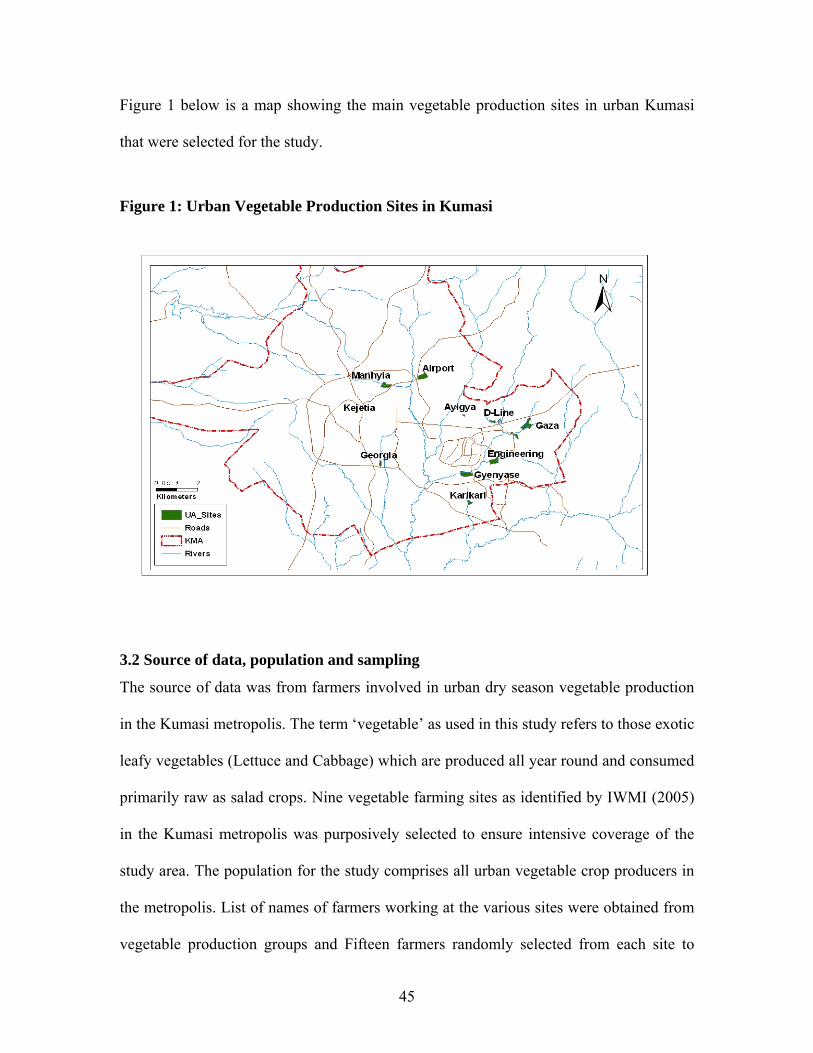
45

Figure 1 below is a map showing the main vegetable production sites in urban Kumasi

that were selected for the study.

Figure 1: Urban Vegetable Production Sites in Kumasi

3.2 Source of data, population and sampling

The source of data was from farmers involved in urban dry season vegetable production

in the Kumasi metropolis. The term ‘vegetable’ as used in this study refers to those exotic

leafy vegetables (Lettuce and Cabbage) which are produced all year round and consumed

primarily raw as salad crops. Nine vegetable farming sites as identified by IWMI (2005)

in the Kumasi metropolis was purposively selected to ensure intensive coverage of the

study area. The population for the study comprises all urban vegetable crop producers in

the metropolis. List of names of farmers working at the various sites were obtained from

vegetable production groups and Fifteen farmers randomly selected from each site to

46

eliminate bias in the sampling process. This gives a sample size of 15 per site and 135-

(15*9) in the whole survey.

3.3 Data collection Techniques

The major instrument for collecting the primary data was a semi-structured questionnaire,

which was administered to vegetable farmers through personal interviews. Secondary

data on existing vegetable production groups and production characteristics of the various

sites were also obtained from IWMI office-Kumasi.

Focus group discussions were organized to investigate farmers’ knowledge and

perceptions regarding the use of untreated water for irrigation, health concerns as well as

the various inputs used and to share ideas to enhance production.

3.4 THEORETICAL FRAMEWORK.

3.4.1 Theory of production and Productive efficiency

The economic theory of production provides the analytical framework for most empirical

research on productivity and efficiency. Productive efficiency means the attainment of a

production goal without a waste. Beginning from this basic idea of ‘‘no waste’’,

economists have built up a variety of theories of efficiency. The fundamental idea

underlying all efficiency measures, however, is that of the quantity of goods and services

per unit of input. Consequently, a production unit is said to be technically inefficient if

too little output is being produced from a given bundle of inputs. There are two basic

methods of measuring efficiency – the classical approach and the frontier approach. The

classical approach is based on the ratio of output to a particular input, and is termed

partial productivity measure.

47

Dissatisfaction with the shortcomings of this approach led economists to develop

advanced econometric and linear programming methods for analysing productivity and

efficiency. The frontier measure of efficiency implies that efficient firms are those

operating on the production frontier. The amount by which a firm lies below its

production frontier is regarded as the measure of inefficiency.

3.4.2 Stochastic Production Frontier (SPF) Analysis and measurement of efficiency

The frontier function approach is a method to measure productive inefficiency of

individual producers. Inefficiency is measured by the deviation from the frontier, which

represent a best-practiced technology among all observed firms.

Coelli (1995) presents two reasons to estimate frontier functions, rather than cost

functions, which are conventionally estimated by OLS method. First, the frontier function

is consistent with theoretical representation of production activities, which is derived

from an optimization process. For example, the production function consists of a series of

outputs attainable, given different combinations of inputs, while cost and profit functions

are represented by frontiers derived from optimization. Second, the estimation of frontier

function provides a tool for measuring the efficiency level of each firm within a given

sample.

The SPF method of analysing efficiency is chosen for this study. The justification is that,

unlike other methods (for example the Data Envelopment Analysis, DEA) the SFP allows

for the sensitivity of data to random shocks by including a conventional random error

48

term in the estimation of the production frontier such that only deviation caused by

controllable decisions are attributed to inefficiency (Jaforullah and Premachandra, 2003).

Inefficiency is assumed to be part of the error term consisting of two parts – a random

error term, which is normally distributed N (0,σ2) and represent random shocks and

statistical errors, and the inefficiency term which is one-sided (non-negative). The

inefficiency error term has a half normal distribution. The SPF is expressed as

Yi = f (Xi,β)ev-u (1)

In logarithm terms the SPF is expressed as

lnYi = ln f (Xi,β) + Vi – Ui (2)

Where Yi is the output vector, Xi is the input vector, β is an unknown parameter vector,

Vi is the random error term assumed to be iid N (0, σ2), Ui is the inefficiency term

independently distributed from Vi.

There is disagreement among econometricians as to the distribution of Ui (Jaforullah and

Premachandra, 2003). Previous studies have used several distributions including single

parameter half-normal distribution, exponential and truncated normal distributions and

two parameter gamma distribution (Jaforullah and Delvin, 1996; Bravo-Ureta and Reiger,

1990; and Sharma et al, 1991). In this study the half normal distribution used by

(Jaforullah and Premachandra, 2003) in a cross sectional data similar to this study will be

adopted.

49

For the technical efficiency of firm i at time t, uit, is transformed as TEit = exp (-ui),

which now represents technical efficiency index. The technical efficiency of the ith firm,

defined by TEi = exp(-ui), has a technical inefficiency effect,ui which is

unobservable.Even if the true value of the parameter vector,β,in the stochastic frontier

model was known, only the difference,εi = vi –ui,could be observed.The best predictor for

ui is the conditional expectation given the value of vi –ui.This result was first recognized

and applied in the stochastic frontier model by Jondrow et al (1982),who derived the

result as follows:

E [ui/ εi] = σλ [ φ(z) – Z]        (3) 1 + λ2 1 - φ(z) Where z = εiλ, φ is read from the normal distribution table. σ An operational predictor of ui involves replacing the unknown parameters with the ML

estimates. Jondrow et al suggested that the technical efficiency of the ith firm should be

predicted using E [ui/ εi]. The rationale for this prediction is that 1 – ui is a first order

approximation to the equation:

exp (-ui) = 1 – ui + ui2/2 –ui

3/6 +…... (4)

After estimating the Uis, firm specific technical efficiency (TE) is then calculated using

the formula:

TE = exp (-ui) = e-ui (5)

The SPF requires the specification of a functional form. Most efficiency studies have

used the Cobb-Douglas production function on the basis of its simplicity (in terms of

analysis and interpretation). But it has been severely criticized for its restrictiveness such

as constant elasticity of substitution and fixed returns to scale, the non compliance of

which can severely affect the results. Based on this, the use of a more flexible function is

50

imperative. Some studies have employed the translog functional form.The translog

function does not establish any restriction beforehand on the elasticity of substitution

between inputs, it does not assume homogeneity or seperablity.Furthermore, the

flexibility of the translog function minimizes the risk of making errors in the

specification.But this functional form has to overcome possible problems of

multicollinearity and degrees of freedom. Generally, the translog function is expressed

as:

ln Yi = β0 + Σiβi lnPi + ΣjβjTj + 1ΣiΣiβii (ln Pi)2 +1ΣjΣjβjj (ln Tj)2

2 2

+ ΣiΣjβij ln PiTj +Vi –Ui (6)

Where Yi is output, Pi and Ti are inputs of variables, Vi is a random error term, Ui is a

measure of inefficiency, βi, βj, βij, βii are unknown parameter estimates.

The above function is assumed to satisfy monotonicity and convexity conditions and such

a functional form may be interpreted as an exact functional form or as a functional form

close to an unknown function obtained as a Taylor’s serial development around an

approximation point. According to research conducted by Denny and Fuss (1977) and

Alvarez (1994), this study has chosen the appropriate functional form obtained by

typifying the variables, that is, by dividing all and each one of the original inputs by their

geometric measures which will facilitate the calculation of the elasticities.

Adopting the above to the peculiarities of cross sectional data, the following model is

suggested:

51

LnYi = ln f (Xi, β) + Vi –Ui (7)

Where Yi is the output vector, Xi is the input vector, β is an unknown parameter vector,

Vi is the random error term assumed to be iid N (0,σ2), Ui is the inefficiency term

independently distributed from Vi and assumes a half-normal distribution.

3.4.3 Analytical Models

For empirical analysis, Cobb-Douglas (1928) stochastic frontier production function will

be estimated. It is vital to note that the Cobb-Douglas frontier is the restricted form of the

translog frontier, in which the second order terms in the translog function are restricted to

be zero.

A Cobb-Douglas production frontier is used to represent the production technology used

by vegetable farmers. In defense of this choice, the following can be said. The Cobb-

Douglas has been the most commonly used function in the specification of and estimation

of production frontiers in empirical studies. It is attractive due to its simplicity and

because of the logarithmic nature of the production function that makes econometric

estimation of the parameters a very simple matter. It is true as Yin (2000) points out, that

this function may be criticized for its restrictive assumptions such as unitary elasticity of

substitution and constant returns to scale and input elasticities, but alternatives such as

translog production functions also have their own limitations such as being susceptible to

multicollinearity and degrees of freedom problems. A study done by Kopp and Smith

(1980) suggests that functional specification has only a small impact on measured

efficiency. Furthermore, Coelli and Perelman (1999) points out that if an industry is not

characterized by perfectly competitive producers, then the use of a Cobb-Douglas

52

functional form is justifiedddd.Considering the fact that the vegetable production industry

in Kumasi is not perfectly competitive, the use of this functional form is justified.

3.4.3 Empirical estimation of Technical efficiency

For our imperical analysis, the Cobb-Douglas frontier production function specifies the

technology of the production process. The variables associated with production are

categorized into output (Y) of lettuce and cabbage in kilograms, Labour (Lab) in

mandays,Quantity of manure / fertilizer (M/F) used in kilograms, Quantity of pesticides

applied in litres,Capital (Cap) used in cedis, and material (Mat) are other inputs measured

as the value of other inputs including fertilizers, manure seeds and pesticides. The model

is defined as:

Y = f (Land, lab, Cap, Mat, Pest, M/F) (8)

The operational Cobb-Douglas stochastic frontier function for lettuce and cabbage

production will be expressed as:

LnY = β0 + β1lnLand + β2lnLab + β3lnCap +β4lnMat +β5lnPest + β6 lnM/F + Ei

(9)

Y is the output, Cap is the value of capital equipments at current cost on the plot, Lab is

the number of mandays of both family and hired labour working on the field, Mat is the

value of other inputs including fertilizers, manure seeds and pesticides, Ei is the

composed error term given as Ei = Vi –Ui, where Vi is the statistical errors and random

shocks such as bad weather, errors in measurement, Ui is the error term measuring the

level of inefficiency in production. The βs represents parameters of linear terms.

53

The technical efficiency of an individual firm is defined in terms of the ratio of observed

output to the corresponding frontier output, conditional on the levels of input used by the

firm. Hence, the technical efficiency of the ith firm is expressed as:

TEi = ln yi / ln y* = (f (xi; β ) exp (vi-ui) / f (xi; β ) exp (vi) (10)

Following Battese and Coelli (1992) the firm specific technical efficiency (TE) can be

evaluated using the conditional expectation of Ui on the random Variable Ei.

TE = exp (-Ui) =e-ui (11)

Such that, 0 ≤ TE ≥ 1

Firm specific technical inefficiency index is then given as

(1 – exp [-Ui]) (12)

If U = 0, it means that vegetable production lies on the stochastic frontier and production

is technically efficient. If U > 0, it implies vegetable production lies below the frontier

and is inefficient. Inefficiency in production could result from the quality and availability

of labour and land, the use of capital and materials, and unhealthy interactions between

these factors.

The explanatory variables to be included in the model are similar to those used in

previous studies of developing country agriculture (Taylor, Drummond and Gomes,

1986; Taylor and Shonkwiler, 1986). A major difference is that we estimate separate

54

production frontiers for two individual crops while most studies rely on estimates of total

value product frontiers.

Estimation of equation (9) was accomplished by maximum likelihood estimation (MLE).

Following Aigner, Lovell, and Schmidt (1977) in which Vi ∼N (0,δv2) and Ui ∼|N

(0,δu2)|, the following log likelihood function could be obtained:

Ln X = Σ ilnLi = Σ i [ -lnδ -1 ln(2 ) –(εi)2 +lnθ (-εδ) ] (13)

2 π δ δ

Where i is the number of observations, δ = (δ2 + δu2)1/2 , λ = δu/δv, εi = vi –ui and θ is

the normal distribution of the function.

3.4.4 Socio-economic model

Average level of technical efficiency measured by mode of truncated normal distribution

(i.e.μit) has been assumed (Dawson, Lingard and Woodford, 1991; Kumbhakar and

Heshmatic, 1995 and Yao and Liu, 1998) to be a function of Socio-economic factors as

shown in the relationship below.

μit = α0 +.α1R1it +α2R2it +α3R3it +α4R4it +α5R5it (14)

Where R1, R2, R3, R4, and R5 are age of farmer, level of education, farming experience,

access to credit and access to off –farm income respectively. These variables are assumed

to influence technical efficiency of the farmers. α0 to α5 are parameters which will be

estimation using OLS.

55

3.4.5 Empirical estimation of Allocative Efficiency of Vegetable production.

Allocative efficiency reflects the ability of a firm to use inputs in optimal proportions,

given their respective prices. A production process is said to be allocatively efficient if it

equates the marginal rate of substitution between each pair of inputs with the input price

ratio. The requirement for the fulfillment of allocative efficiency is for the marginal

physical product (MPP) of all productive resources to be known (Ellis, 1988). The aim of

this study is to estimate the allocative efficiencies of labour and Capital since it is these

factors that are substituted for in the production process.

From the cobb-Duaglas function presented in equation 8, the factor elasticities of labour

and capital (ELand EK, respectively) are obtained directly from the equation. The

estimation process is based on the allocative efficiency rule which states that the slop e of

the production function (MPP) should equal the inverse ratio of input price to output

price at the point of profit maximization (Ellis, 1988).

MPPi = w (15)

Py

W is the wage rate, Py is the price of output (Lettuce).Cross multiplying yields

MPL. Py = MVPL = w (16)

MVPL = 1 (17)

w

56

That is, the marginal value product of the variable input divided by the input price should

equal one. This is the allocative efficiency index (Z) for a single input given by

Z = MVPx (18) for any variable X

Py

Similarly, for capital,

Z = MVPK (19) k is the unit price of capital. Py The marginal products will be calculated as follows: MPL = µYi * EL (20) of labour µXi MPL = µYi * Ek (21) µXi for Capital The allocative efficiency ratios are then expressed as Z = MPL * Py (22) for labour input W Z = MPK * Py (23) for capital input W

Where MPL, MPK are the marginal products of labour and capital respectively,µYi and

µXi are the arithmetic means (logs) of the output and inputs respectively of the

production process.

If Z =1, it implies that the input is utilized efficiently

If Z > 1,it implies an underutilization of the factor input

If Z < 1, it implies an over utilization of the factor input.

57

3.5 Hypothesis Testing

For the frontier model, the null hypothesis that there are no technical inefficiency effects

in the model can be conducted by testing the null and the alternative hypothesis Ho:γ = 0

against H1: γ > 0 .The Wald statistic can be used to test the hypothesis. For the Wald test,

the ratio of the estimate for γ to its estimated standard error is calculated. If Ho:γ = 0 is

true, this statistic is asymptotically distributed as a standard normal random variable.

However, the test must be performed as a one-sided test because γ cannot take negative

values. For the fact that the Wald test is handicapped by its poor size properties, Coelli

(1995) suggested that the generalized likelihood-ratio test should be performed when ML

estimation is involved because this test has the correct size. However, difficulties arise in

testing Ho:γ = 0 because: γ = 0 lies on the boundary of the parameter space for γ. Coelli

(1995) recommended the one-sided generalized likelihood ratio test of size α which says:

Reject Ho:γ = 0 in favor of H1: γ > 0 if λ exceedsχ22(α).The value for a test of size α=

0.05, is 2.706 [table 1of Kodde and Palm, (1986)].

The first hypothesis which specifies that the sample enterprises are technically efficient

will be tested using the generalized likelihood ratio test statistic, which is defined by:

λ = -2 ln [L (Ho) /L (H1)] (24)

Where L (Ho) is the value of the likelihood function for the frontier model, in which the

parameter restrictions specified by the null hypothesis, Ho, are imposed, and H1 is the

value of the likelihood function for the general frontier model. If the null hypothesis is

true, the λ has approximately chi-square (or mixed square) distribution with degrees of

58

freedom equal to the difference between the parameters estimated under H1 and Ho,

respectively. The second hypothesis will be tested using the ratio of the estimated

coefficient of the policy variables to the standard error.

3.6 Estimation of stochastic Frontier and Technical Inefficiency functions.

The estimation was carried out in three steps. First, Ordinary least squares (OLS)

estimation of the Stochastic Frontier production function yields estimates of β

coefficients. All the estimates except the one for the intercept, βo are biased. Second a

grid search finds γ using the OLS estimates of βo and σ2 which are adjusted according to

the corrected Ordinary least squares formula presented in Coelli (1995). The coefficients,

δ are set to zero and γ is limited between zero and one and defined as:

γ = σ2u / σ2 (25)

The regression is estimated using the values selected in the grid search as starting values

in an iterative procedure to obtain the final ML estimates of the coefficients β and δ,

together with the variance parameters that are expressed as:

σ2 = σ2v + σ2 u (26)

The ML estimates for the parameters of the Stochastic frontier model and the predicted

technical and allocative efficiency estimates were obtained by using the computer

Programme, Lindep Version 7.0, in which the variance parameters are expressed in

terms of: γ = σ2u / σ2 and σ2 = σ2

v + σ2 u Coelli (1996).

3.7 Definition of Variables

It is argued that the productivity of any enterprise depends on labour and capital.

Productivity measurement of outputs, therefore, is a means of quantifying the efficiency

59

with which these inputs are utilized in the production processes a measure of the output

of a firm, effective inputs will be considered for this study. In this study, environmental

and social effects are not considered as having impact on input use since the main

concern is to find out the inefficiency in utilizing the labour and other inputs considered

in the production process.

3.7.1 List of variables

Output, input and cost variables associated with dry season vegetable production have

been identified. Other variables such as age, education etc relate to policy influences that

can enhance the efficiency of the firm will be gathered.

3.7.2 Inputs

Land: area devoted to Cabbage and Lettuce production (hacters) per season.

Labour: Sum of family and hired labour measured in man -days, one man-day is

equivalent to 8 hours in this study.

Manure / fertilizer: The quantity of manure /fertilizer in kilograms applied per hectare in

a season

Insecticides: The volume of insecticides (in Liters) used per hectare in a season

Material: refers to all cash expenses (Variable cost) incurred in producing an output in a

season. Material consists of cost of seeds, cost of fertilizer / manure, cost of insecticides,

and other service charges. The measuring unit of material is in cedis.

Capital refers to the value of equipments at current cost used in production.

60

3.7.3 Determinants of efficiency.

R1 = Age of farmer

R2 = Level of education of farmer / decision maker

R3 = years of farming experience (vegetables only)

R4 = Access to credit during the cropping season

R5 = access to off-farm income

61

CHAPTER FOUR

RESULTS AND DISCUSSION

4.0 Introduction This chapter presents a discussion of the results. Results on the technical and allocative

efficiencies of vegetable production are presented and discussed. The results on factors

influencing technical efficiency, productivity of land and labour and the problems of

marketing vegetables are also presented and discussed. Finally, the perception of farmers

on untreated water use are identified and analyzed.

4.1.1: Estimates of the production frontier function

The estimation of the relative efficiency of production units is conducted by assuming the

appropriateness of the log-linear Cobb-Douglas case. The specification of the translog

function was also tested. The results of the translog function is not reported in this study

because it did not have the right signs for the coefficients and almost all the variables

included in the model were found not to be significant. Thus, the specification using the

translog function to represent the production technology was not appropriate. Results of

the Cobb-Douglas gave the best estimates and hence the choice for it.

All the estimations were done using maximum likelihood methods from the statistical

programme LINDEP Version 7.0.The goodness of fit of the estimated regression

equations evaluated by R2 for the OLS looks low. The poor R2 value may be accounted

for by the fact that outliers existed. Apart from these outliers, The R2 value implies that

the inputs to the model do statistically explain the model output. In addition, the F-

Statistic of 11.33 shows that the relationship between the variables are significant at 1%

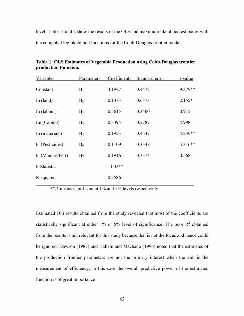
62

level. Tables 1 and 2 show the results of the OLS and maximum likelihood estimates with

the computed log likelihood functions for the Cobb-Douglas frontier model.

Table 1: OLS Estimates of Vegetable Production using Cobb-Douglas frontier production Function. Variables Parameters Coefficients Standard error t-value Constant B1 4.1947 0.4472 9.379** In (land) B2 0.1373 0.6373 2.155* In (labour) B3 0.3615 0.3400 0.915 Ln (Capital) B4 0.3395 0.2787 4.998 In (materials) B4 0.1923 0.4537 4.239** ln (Pesticides) B6 0.1109 0.3348 3.316** ln (Manure/Fert) B7 0.1916 0.3374 0.568 F-Statistic 11.33** R-squared 0.2586 **,* means significant at 1% and 5% levels respectively

Estimated OlS results obtained from the study revealed that most of the coefficients are

statistically significant at either 1% or 5% level of significance. The poor R2 obtained

from the results is not relevant for this study because that is not the focus and hence could

be ignored. Dawson (1987) and Hallam and Machado (1996) noted that the estimates of

the production frontier parameters are not the primary interest when the aim is the

measurement of efficiency; in this case the overall predictive power of the estimated

function is of great importance

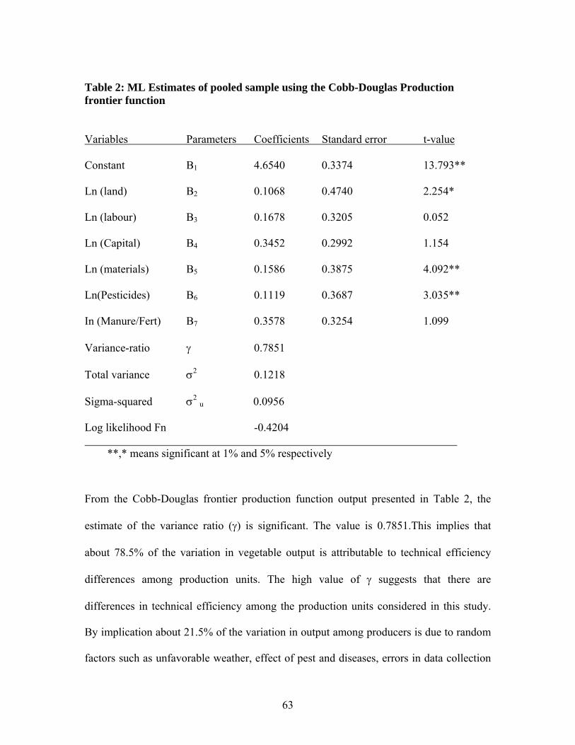
63

Table 2: ML Estimates of pooled sample using the Cobb-Douglas Production frontier function Variables Parameters Coefficients Standard error t-value Constant B1 4.6540 0.3374 13.793** Ln (land) B2 0.1068 0.4740 2.254* Ln (labour) B3 0.1678 0.3205 0.052 Ln (Capital) B4 0.3452 0.2992 1.154 Ln (materials) B5 0.1586 0.3875 4.092** Ln(Pesticides) B6 0.1119 0.3687 3.035** In (Manure/Fert) B7 0.3578 0.3254 1.099 Variance-ratio γ 0.7851 Total variance σ2 0.1218 Sigma-squared σ2 u 0.0956 Log likelihood Fn -0.4204 **,* means significant at 1% and 5% respectively

From the Cobb-Douglas frontier production function output presented in Table 2, the

estimate of the variance ratio (γ) is significant. The value is 0.7851.This implies that

about 78.5% of the variation in vegetable output is attributable to technical efficiency

differences among production units. The high value of γ suggests that there are

differences in technical efficiency among the production units considered in this study.

By implication about 21.5% of the variation in output among producers is due to random

factors such as unfavorable weather, effect of pest and diseases, errors in data collection

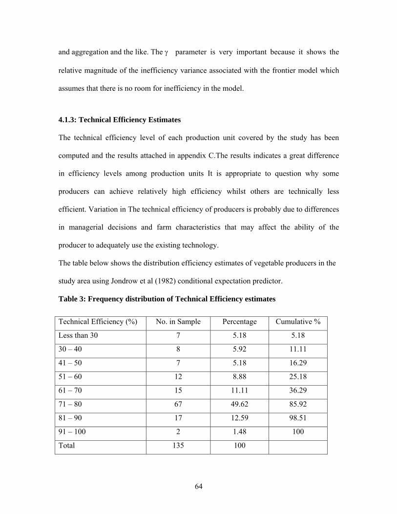
64

and aggregation and the like. The γ parameter is very important because it shows the

relative magnitude of the inefficiency variance associated with the frontier model which

assumes that there is no room for inefficiency in the model.

4.1.3: Technical Efficiency Estimates

The technical efficiency level of each production unit covered by the study has been

computed and the results attached in appendix C.The results indicates a great difference

in efficiency levels among production units It is appropriate to question why some

producers can achieve relatively high efficiency whilst others are technically less

efficient. Variation in The technical efficiency of producers is probably due to differences

in managerial decisions and farm characteristics that may affect the ability of the

producer to adequately use the existing technology.

The table below shows the distribution efficiency estimates of vegetable producers in the

study area using Jondrow et al (1982) conditional expectation predictor.

Table 3: Frequency distribution of Technical Efficiency estimates

Technical Efficiency (%) No. in Sample Percentage Cumulative %

Less than 30 7 5.18 5.18

30 – 40 8 5.92 11.11

41 – 50 7 5.18 16.29

51 – 60 12 8.88 25.18

61 – 70 15 11.11 36.29

71 – 80 67 49.62 85.92

81 – 90 17 12.59 98.51

91 – 100 2 1.48 100

Total 135 100

65

The study shows that technical efficiency ranges between 21.9% - 95.02%.The lowest

level of efficiency is 21.9% which is far below the efficient frontier by 78.1%.Such

production units are technically inefficient. The highest level of efficiency is 95.02%

which is only 4.98% away from the frontier. Such production units can be classified as

being technically efficient since in reality production units hardly operate at 100% level

of efficiency. The mean technical efficiency of the pooled sample is 66.67%.This

compares favorably with other efficiency studies conducted in other areas of agriculture.

For instance, previous studies in rice had 65% (Kalirajan and Shand, 1986); 75%

(Kumbhakar, 1994); 50% (Kalirajan and Flinn, 1983); 59% (Bravo-ureta and Evenson,

1993) and 66% (Pierani and Rizzi, 2002).

The 66.67% mean technical efficiency implies that on the average, 33.33% more output

would have been produced with the same level of inputs if producers were to produce on

the most efficient frontier following best practices. A greater proportion of the production

units (49.6%) are concentrated in the efficiency class of 71 – 80%.The next highest

concentration of producers’ the efficiency class 81 – 90% which contains 12.59% of the

pooled sample.

4.1.4 Hypothesis Testing

The null hypothesis of the study stipulates that there is no technical difference among the

sampled vegetable farmers. To test the null hypothesis, the logarithmic likelihood

function on the Cobb –Douglas frontier is compared to that of the traditional production

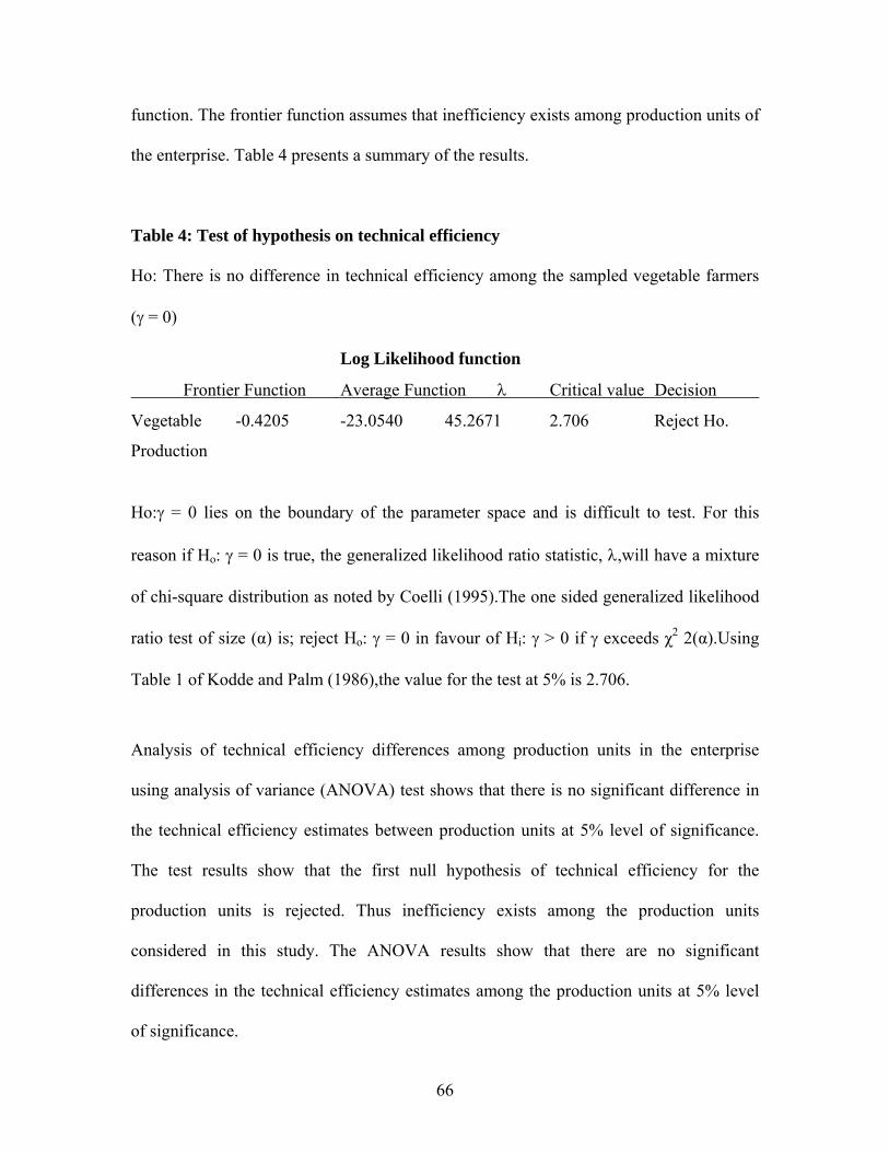
66

function. The frontier function assumes that inefficiency exists among production units of

the enterprise. Table 4 presents a summary of the results.

Table 4: Test of hypothesis on technical efficiency

Ho: There is no difference in technical efficiency among the sampled vegetable farmers

(γ = 0)

Log Likelihood function

Frontier Function Average Function λ Critical value Decision

Vegetable -0.4205 -23.0540 45.2671 2.706 Reject Ho.

Production

Ho:γ = 0 lies on the boundary of the parameter space and is difficult to test. For this

reason if Ho: γ = 0 is true, the generalized likelihood ratio statistic, λ,will have a mixture

of chi-square distribution as noted by Coelli (1995).The one sided generalized likelihood

ratio test of size (α) is; reject Ho: γ = 0 in favour of Hi: γ > 0 if γ exceeds χ2 2(α).Using

Table 1 of Kodde and Palm (1986),the value for the test at 5% is 2.706.

Analysis of technical efficiency differences among production units in the enterprise

using analysis of variance (ANOVA) test shows that there is no significant difference in

the technical efficiency estimates between production units at 5% level of significance.

The test results show that the first null hypothesis of technical efficiency for the

production units is rejected. Thus inefficiency exists among the production units

considered in this study. The ANOVA results show that there are no significant

differences in the technical efficiency estimates among the production units at 5% level

of significance.

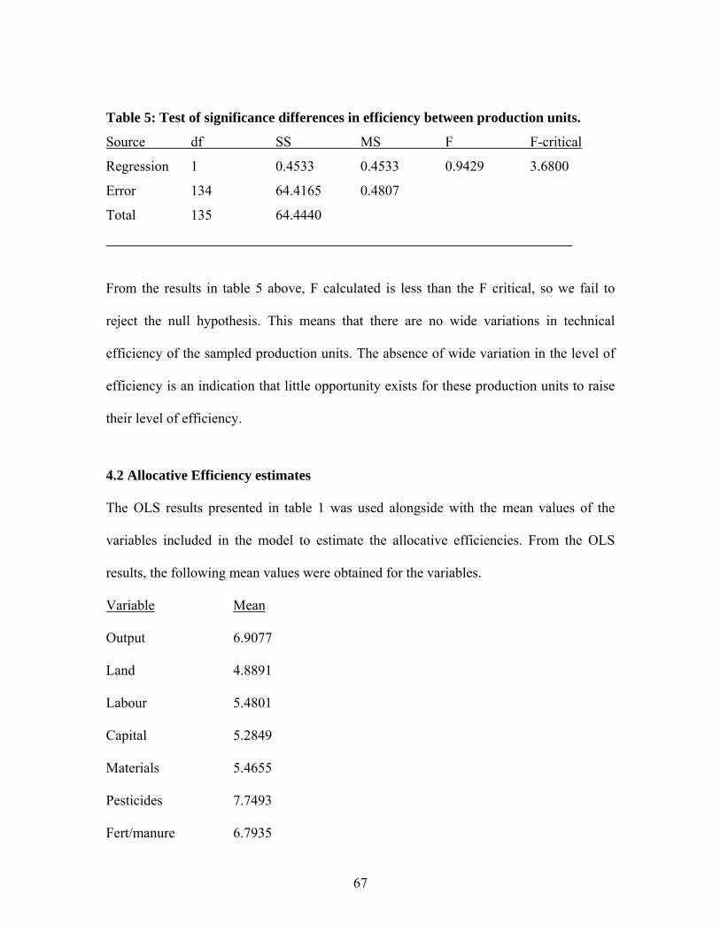
67

Table 5: Test of significance differences in efficiency between production units.

Source df SS MS F F-critical

Regression 1 0.4533 0.4533 0.9429 3.6800

Error 134 64.4165 0.4807

Total 135 64.4440

From the results in table 5 above, F calculated is less than the F critical, so we fail to

reject the null hypothesis. This means that there are no wide variations in technical

efficiency of the sampled production units. The absence of wide variation in the level of

efficiency is an indication that little opportunity exists for these production units to raise

their level of efficiency.

4.2 Allocative Efficiency estimates

The OLS results presented in table 1 was used alongside with the mean values of the

variables included in the model to estimate the allocative efficiencies. From the OLS

results, the following mean values were obtained for the variables.

Variable Mean

Output 6.9077

Land 4.8891

Labour 5.4801

Capital 5.2849

Materials 5.4655

Pesticides 7.7493

Fert/manure 6.7935

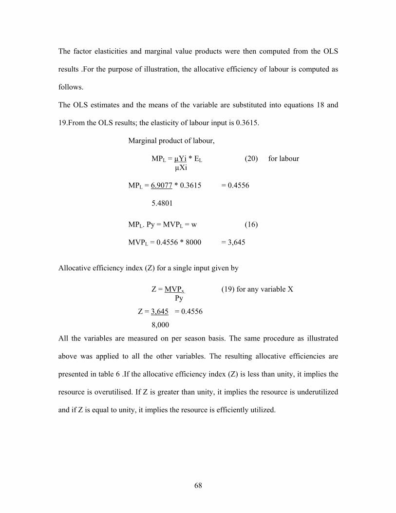
68

The factor elasticities and marginal value products were then computed from the OLS

results .For the purpose of illustration, the allocative efficiency of labour is computed as

follows.

The OLS estimates and the means of the variable are substituted into equations 18 and

19.From the OLS results; the elasticity of labour input is 0.3615.

Marginal product of labour,

MPL = µYi * EL (20) for labour µXi MPL = 6.9077 * 0.3615 = 0.4556 5.4801

MPL. Py = MVPL = w (16)

MVPL = 0.4556 * 8000 = 3,645

Allocative efficiency index (Z) for a single input given by

Z = MVPx (19) for any variable X Py

Z = 3,645 = 0.4556

8,000

All the variables are measured on per season basis. The same procedure as illustrated

above was applied to all the other variables. The resulting allocative efficiencies are

presented in table 6 .If the allocative efficiency index (Z) is less than unity, it implies the

resource is overutilised. If Z is greater than unity, it implies the resource is underutilized

and if Z is equal to unity, it implies the resource is efficiently utilized.

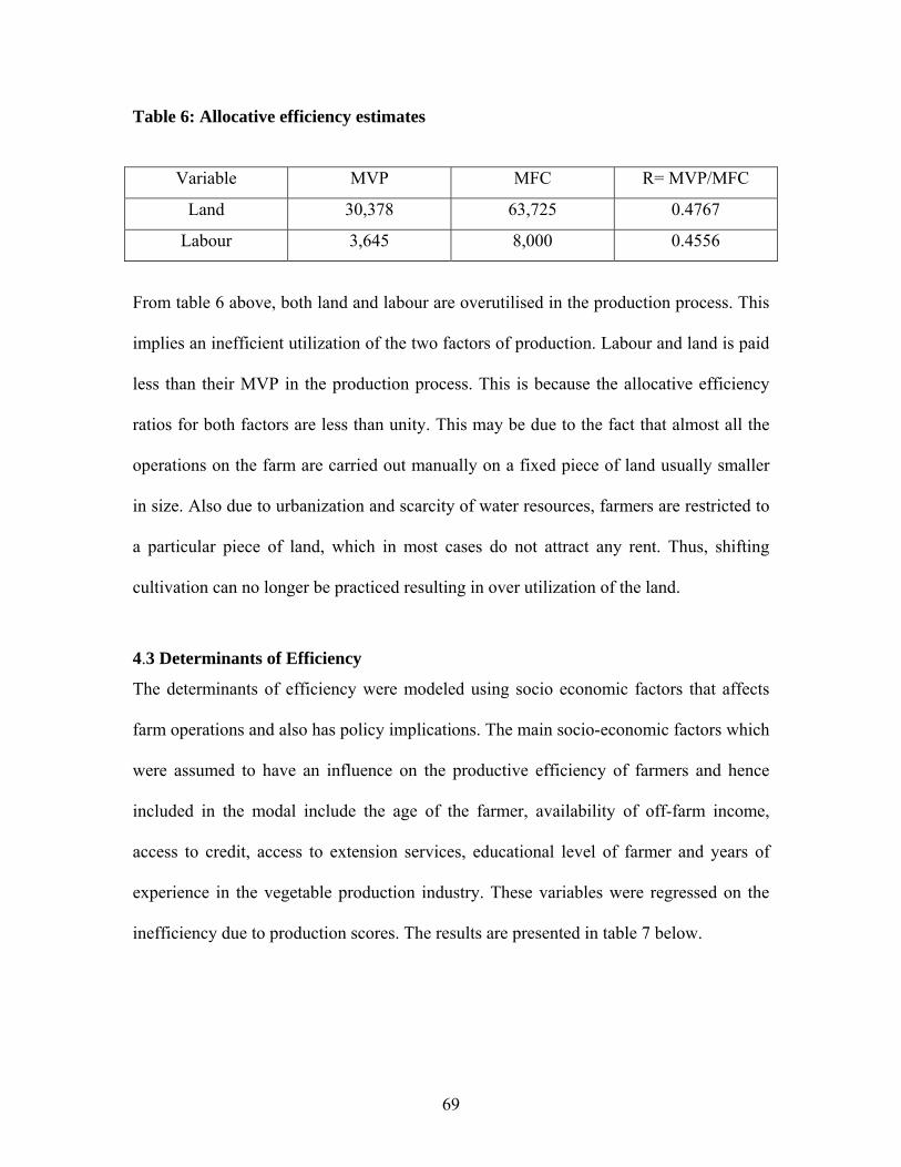
69

Table 6: Allocative efficiency estimates

Variable MVP MFC R= MVP/MFC

Land 30,378 63,725 0.4767

Labour 3,645 8,000 0.4556

From table 6 above, both land and labour are overutilised in the production process. This

implies an inefficient utilization of the two factors of production. Labour and land is paid

less than their MVP in the production process. This is because the allocative efficiency

ratios for both factors are less than unity. This may be due to the fact that almost all the

operations on the farm are carried out manually on a fixed piece of land usually smaller

in size. Also due to urbanization and scarcity of water resources, farmers are restricted to

a particular piece of land, which in most cases do not attract any rent. Thus, shifting

cultivation can no longer be practiced resulting in over utilization of the land.

4.3 Determinants of Efficiency

The determinants of efficiency were modeled using socio economic factors that affects

farm operations and also has policy implications. The main socio-economic factors which

were assumed to have an influence on the productive efficiency of farmers and hence

included in the modal include the age of the farmer, availability of off-farm income,

access to credit, access to extension services, educational level of farmer and years of

experience in the vegetable production industry. These variables were regressed on the

inefficiency due to production scores. The results are presented in table 7 below.

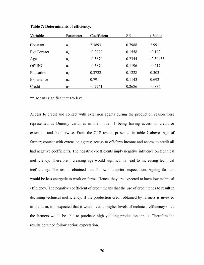
70

Table 7: Determinants of efficiency.

Variable Parameter Coefficient SE t-Value

Constant α1 2.3893 0.7988 2.991

Ext.Contact α2 -0.2990 0.1558 -0.192

Age α3 -0.5870 0.2344 -2.504**

Off INC α4 -0.5870 0.1196 -0.217

Education α5 0.3722 0.1228 0.303

Experience α6 0.7911 0.1143 0.692

Credit α7 -0.2241 0.2686 -0.835

**, Means significant at 1% level.

Access to credit and contact with extension agents during the production season were

represented as Dummy variables in the model; 1 being having access to credit or

extension and 0 otherwise. From the OLS results presented in table 7 above, Age of

farmer; contact with extension agents; access to off-farm income and access to credit all

had negative coefficients. The negative coefficients imply negative influence on technical

inefficiency. Therefore increasing age would significantly lead to increasing technical

inefficiency. The results obtained here follow the apriori expectation. Ageing farmers

would be less energetic to work on farms. Hence, they are expected to have low technical

efficiency. The negative coefficient of credit means that the use of credit tends to result in

declining technical inefficiency. If the production credit obtained by farmers is invested

in the farm, it is expected that it would lead to higher levels of technical efficiency since

the farmers would be able to purchase high yielding production inputs. Therefore the

results obtained follow apriori expectation.

71

The positive coefficients obtained for level of education, and years of farming experience

also follows apriori expectation, given that educational is an important factor in

technology adoption. Educated farmers are expected to be receptive to improved farming

techniques and therefore should have a higher level of technical efficiency than farmers

with less education. The positive coefficient of education is in line with the findings of

previous studies by Obwona ,2000; Sidhu and Baanate, 1981; Jamison and Lau, 1982;

Pudasaini, 1983) that education has a positive effect on profits, a result that indicates the

existence of management related inefficiency (Ali and Byerlee, 1991).

Farming experience having positive coefficient indicates that farming experience would

lead to an increase in technical efficiency. This result has also confirmed apriori

expectation. More experienced farmers are expected to have higher level of technical

efficiency than farmers with low farming experience, given that farming business

involves annual routine activity.

Even though from theory access to credit, availability of off-farm income, contact with

extension agents and years of production experience are expected to impact significantly

on the productive efficiency of farmers, the results obtained from this study is at variance

with it. This is explained by the fact that only a small proportion of the respondents had

access to these services. Majority of the respondents (59%) did not achieve basic

education required to enhance their efficiency. Only 4.44% of the respondents had

tertiary education and 36.3% had secondary education (JSS & SSS). Also, only 7.4% of

the respondents had access to credit; 15.5%had access to extension services; and 29.6%

had access to off-farm income.

72

The age of the farmer was found to be highly significantly related to productive

efficiency at the 1% level of significance. This is explained by the fact that majority of

the respondents covered by the study were between the ages of 18 –39 required to boast

agricultural production. They are described as being energetic, smart to adopt new

technologies and market oriented in production. This therefore enhances their chances of

being efficient in the production process. The study revealed that 76.3% of the

respondents were between the ages of 18-39years; 20% were between 40 – 49years and

only 3.7% was fifty years and above old. This therefore suggests a greater potential to

make the vegetable industry more efficient.

Due to the youthful nature of the age structure of the respondents, the number of years

that farmers had been in production was very less. Since majority of the respondents were

youthful with few years of experience in the vegetable production industry, the study

found years of experience in production not to be significantly related to productive

efficiency.

4.4 Productivity of land and labour

Partial productivity measures for individual inputs were estimated. The parameters

estimated from the field as attached in appendix C is used in calculating the productivity

of various factors of production in the production process. The productivity of land is the

ratio of gross revenue obtained from production to the land area put under cultivation.

The productivity of land was determined for all the nine sites covered by the study.

Productivity of land varies from ¢72,386,587/ha to ¢140,325,417/ha. The highest

productivity of land is found at Georgia. This could be explained by the fact that it is

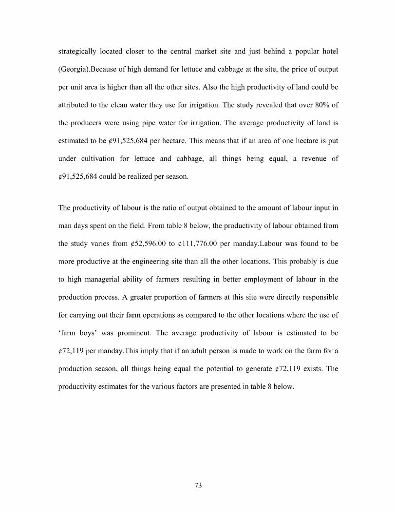
73

strategically located closer to the central market site and just behind a popular hotel

(Georgia).Because of high demand for lettuce and cabbage at the site, the price of output

per unit area is higher than all the other sites. Also the high productivity of land could be

attributed to the clean water they use for irrigation. The study revealed that over 80% of

the producers were using pipe water for irrigation. The average productivity of land is

estimated to be ¢91,525,684 per hectare. This means that if an area of one hectare is put

under cultivation for lettuce and cabbage, all things being equal, a revenue of

¢91,525,684 could be realized per season.

The productivity of labour is the ratio of output obtained to the amount of labour input in

man days spent on the field. From table 8 below, the productivity of labour obtained from

the study varies from ¢52,596.00 to ¢111,776.00 per manday.Labour was found to be

more productive at the engineering site than all the other locations. This probably is due

to high managerial ability of farmers resulting in better employment of labour in the

production process. A greater proportion of farmers at this site were directly responsible

for carrying out their farm operations as compared to the other locations where the use of

‘farm boys’ was prominent. The average productivity of labour is estimated to be

¢72,119 per manday.This imply that if an adult person is made to work on the farm for a

production season, all things being equal the potential to generate ¢72,119 exists. The

productivity estimates for the various factors are presented in table 8 below.

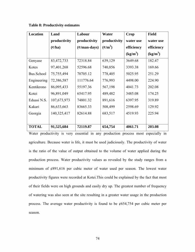
74

Table 8: Productivity estimates Location Land

productivity

(¢/ha)

Labour

productivity

(¢/man-days)

Water

productivity

(¢/m3)

Crop

water use

efficiency

(kg/m3)

Field

water use

efficiency

(kg/m3)

Genyase

Kotes

Bus.School

Engineering

Kentikrono

Kotei

Eduasi N.S.

Kakari

Georgia

83,472,733

97,401,268

75,755,494

72,386,587

86,095,433

96,891,049

107,673,973

86,633,663

140,325,417

72318.84

52596.68

70705.12

111776.64

55197.36

65417.95

74801.32

83665.33

82614.88

639,129

740,856

778,405

776,993

567,198

489,482

891,616

508,499

683,517

3649.68

3393.38

5025.95

4498.00

4041.73

3485.08

6397.95

2598.69

4519.93

182.47

169.66

251.29

224.90

202.08

174.25

319.89

129.92

225.94

TOTAL 91,525,684 72119.87 654,754 4061.71 203.08

Water productivity is very essential in any production process most especially in

agriculture. Because water is life, it must be used judiciously. The productivity of water

is the ratio of the value of output obtained to the volume of water applied during the

production process. Water productivity values as revealed by the study ranges from a

minimum of ¢891,616 per cubic meter of water used per season. The lowest water

productivity figures were recorded at Kotei.This could be explained by the fact that most

of their fields were on high grounds and easily dry up. The greatest number of frequency

of watering was also seen at the site resulting in a greater water usage in the production

process. The average water productivity is found to be ¢654,754 per cubic meter per

season.

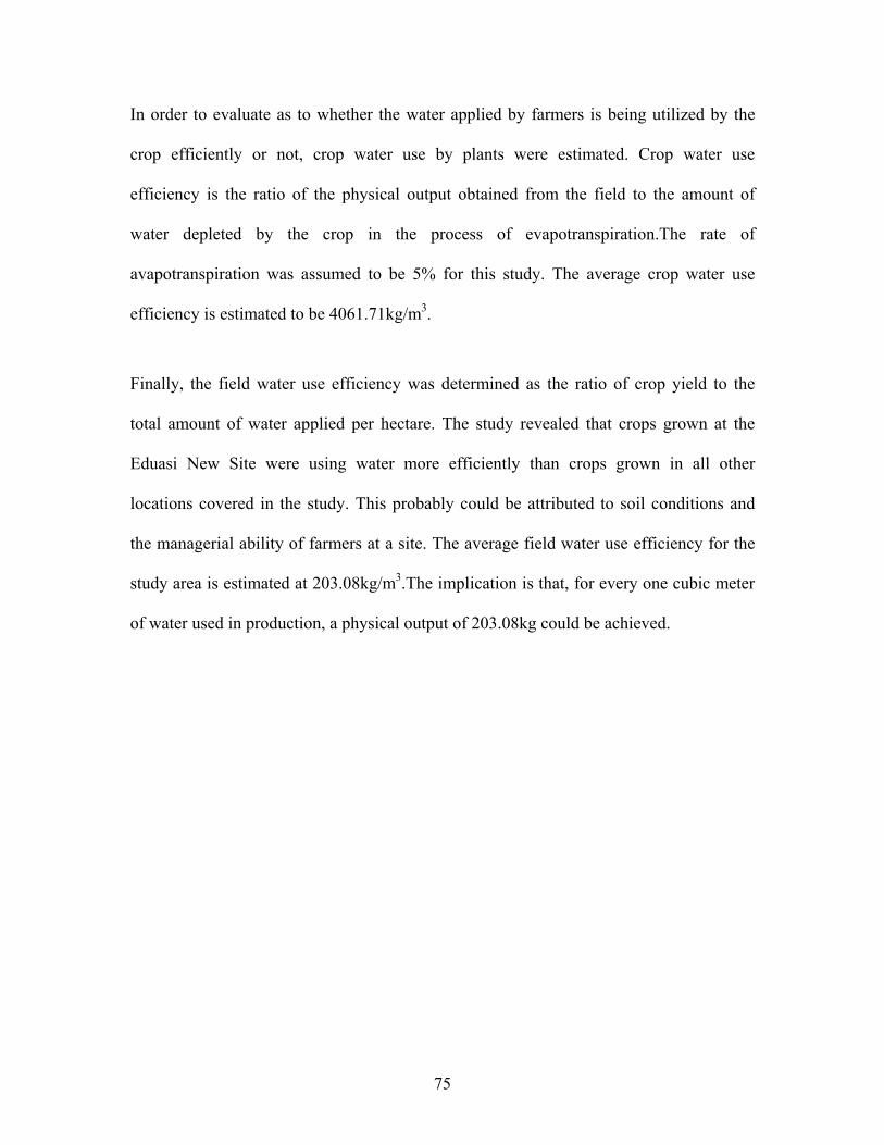
75

In order to evaluate as to whether the water applied by farmers is being utilized by the

crop efficiently or not, crop water use by plants were estimated. Crop water use

efficiency is the ratio of the physical output obtained from the field to the amount of

water depleted by the crop in the process of evapotranspiration.The rate of

avapotranspiration was assumed to be 5% for this study. The average crop water use

efficiency is estimated to be 4061.71kg/m3.

Finally, the field water use efficiency was determined as the ratio of crop yield to the

total amount of water applied per hectare. The study revealed that crops grown at the

Eduasi New Site were using water more efficiently than crops grown in all other

locations covered in the study. This probably could be attributed to soil conditions and

the managerial ability of farmers at a site. The average field water use efficiency for the

study area is estimated at 203.08kg/m3.The implication is that, for every one cubic meter

of water used in production, a physical output of 203.08kg could be achieved.

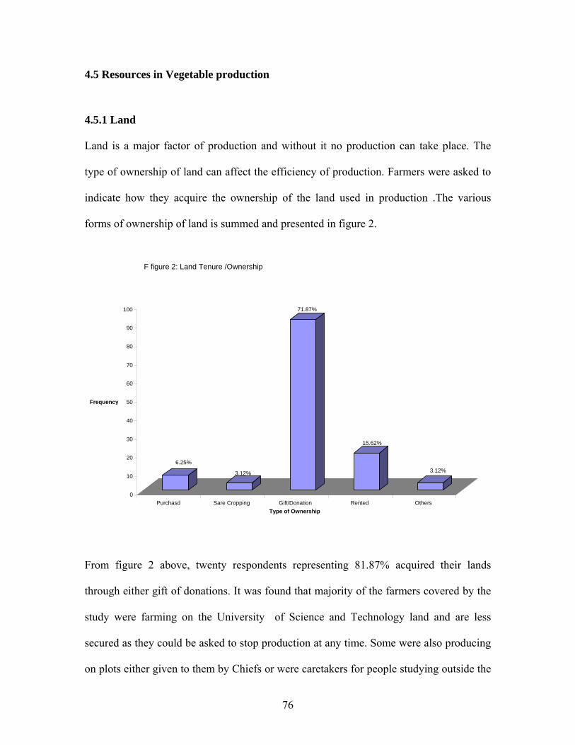
76

4.5 Resources in Vegetable production

4.5.1 Land

Land is a major factor of production and without it no production can take place. The

type of ownership of land can affect the efficiency of production. Farmers were asked to

indicate how they acquire the ownership of the land used in production .The various

forms of ownership of land is summed and presented in figure 2.

From figure 2 above, twenty respondents representing 81.87% acquired their lands

through either gift of donations. It was found that majority of the farmers covered by the

study were farming on the University of Science and Technology land and are less

secured as they could be asked to stop production at any time. Some were also producing

on plots either given to them by Chiefs or were caretakers for people studying outside the

0

10

20

30

40

50

60

70

80

90

100

Frequency

Purchasd Sare Cropping Gift/Donation Rented OthersType of Ownership

F figure 2: Land Tenure /Ownership

71.87%

6.25%

3.12%

15.62%

3.12%

77

region or abroad. The implication is that, the development of permanent structures such

as wells to ensure all year round production and enhance efficiency in production cannot

be achieved. About 3.12% of the respondents were practicing share cropping system.

Under this arrangement, land owners are allocated a specified number of beds in every

production season. This system is mostly practiced at Kentikrono area. Almost all the

farmers who had their lands through this arrangement were migrants from Northern

Ghana specifically Upper East Region. One quarter of the number of beds produced per

season goes to the land owner while three-quarters is for the farmer.

About 6.25% of the respondents had their lands through purchase. The average amount

paid for an area of 10,000m2 varies from ¢3,000,000 to ¢12,000,000 cedis.Only 3.12% of

the respondents hand their lands through inheritance.

In general, over 80% of vegetable producers covered by the study do not owe land

permanently to undertake any meaningful production. The implication is that,

investments made in developing the land is minimal or non-existent, permanent farm

structures cannot be erected and the future of the vegetable industry is uncertain though it

proof profitable to most farmers.

4.5.2 Water

4.5.2.1 Sources of water used in Irrigation

The use of untreated water in agriculture is growing due to water scarcity, population

growth and urbanization which all lead to the generation of yet more wastewater in urban

areas. Farmers in the Kumasi metropolis use a variety of water sources for irrigation. Out

of the total number of respondents covered by the study, 9.62% were using the same

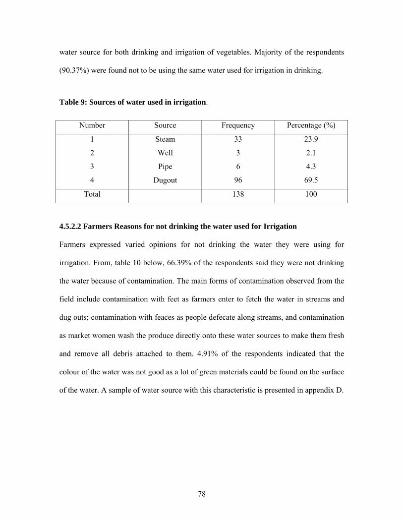
78

water source for both drinking and irrigation of vegetables. Majority of the respondents

(90.37%) were found not to be using the same water used for irrigation in drinking.

Table 9: Sources of water used in irrigation.

Number Source Frequency Percentage (%)

1

2

3

4

Steam

Well

Pipe

Dugout

33

3

6

96

23.9

2.1

4.3

69.5

Total 138 100

4.5.2.2 Farmers Reasons for not drinking the water used for Irrigation

Farmers expressed varied opinions for not drinking the water they were using for

irrigation. From, table 10 below, 66.39% of the respondents said they were not drinking

the water because of contamination. The main forms of contamination observed from the

field include contamination with feet as farmers enter to fetch the water in streams and

dug outs; contamination with feaces as people defecate along streams, and contamination

as market women wash the produce directly onto these water sources to make them fresh

and remove all debris attached to them. 4.91% of the respondents indicated that the

colour of the water was not good as a lot of green materials could be found on the surface

of the water. A sample of water source with this characteristic is presented in appendix D.

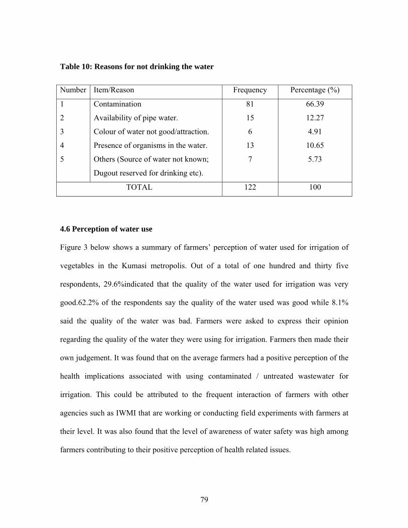
79

Table 10: Reasons for not drinking the water

Number Item/Reason Frequency Percentage (%)

1

2

3

4

5

Contamination

Availability of pipe water.

Colour of water not good/attraction.

Presence of organisms in the water.

Others (Source of water not known;

Dugout reserved for drinking etc).

81

15

6

13

7

66.39

12.27

4.91

10.65

5.73

TOTAL 122 100

4.6 Perception of water use Figure 3 below shows a summary of farmers’ perception of water used for irrigation of

vegetables in the Kumasi metropolis. Out of a total of one hundred and thirty five

respondents, 29.6%indicated that the quality of the water used for irrigation was very

good.62.2% of the respondents say the quality of the water used was good while 8.1%

said the quality of the water was bad. Farmers were asked to express their opinion

regarding the quality of the water they were using for irrigation. Farmers then made their

own judgement. It was found that on the average farmers had a positive perception of the

health implications associated with using contaminated / untreated wastewater for

irrigation. This could be attributed to the frequent interaction of farmers with other

agencies such as IWMI that are working or conducting field experiments with farmers at

their level. It was also found that the level of awareness of water safety was high among

farmers contributing to their positive perception of health related issues.

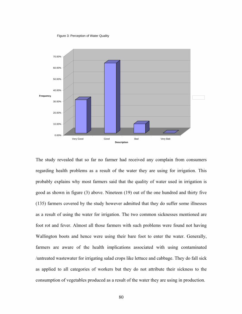
80

The study revealed that so far no farmer had received any complain from consumers

regarding health problems as a result of the water they are using for irrigation. This

probably explains why most farmers said that the quality of water used in irrigation is

good as shown in figure (3) above. Nineteen (19) out of the one hundred and thirty five

(135) farmers covered by the study however admitted that they do suffer some illnesses

as a result of using the water for irrigation. The two common sicknesses mentioned are

foot rot and fever. Almost all those farmers with such problems were found not having

Wallington boots and hence were using their bare foot to enter the water. Generally,

farmers are aware of the health implications associated with using contaminated

/untreated wastewater for irrigating salad crops like lettuce and cabbage. They do fall sick

as applied to all categories of workers but they do not attribute their sickness to the

consumption of vegetables produced as a result of the water they are using in production.

0.00%

10.00%

20.00%

30.00%

40.00%

50.00%

60.00%

70.00%

Frequency

Very Good Good Bad Very BabDescription

Figure 3: Perception of Water Quality

81

4.7 Marketing of Vegetables.

The study revealed that all the farmers covered by the study sell their produce at the farm

gate level through market women. Farmers in the study area are therefore restricted to a

single channel through which they sell their produce. Hundred percent of the farmers

covered were found to be selling their produce through market women. When asked why

they could not go to the central market and sell directly to individuals and other

organizations, varied responses were given . The main reasons offered by farmers

include the intensive nature of their farm operations which may not allow them time to

wait and make sales at the market; Creating jobs for others (market women) ; and

difficulty in selling the produce at the desired price because of collusive behavior of

market women.

4.7.1 Problems of marketing Lettuce and Cabbage.

Table 9 presents the main problems encountered by vegetable farmers in the production

process. In most developing countries production is not much of a problem but rather

marketing. Farmers were asked to state at least two most pressing problems in order of

priority facing them relating to marketing of their produce. The main problems raised is

summarized and presented below.

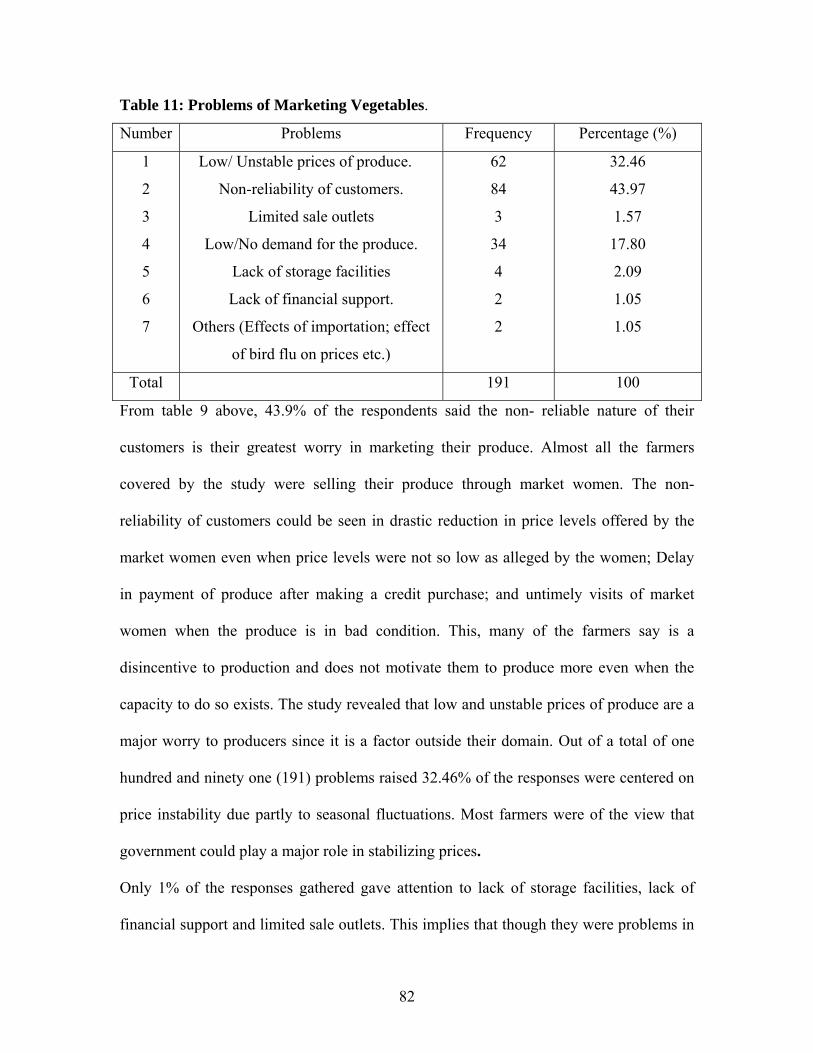
82

Table 11: Problems of Marketing Vegetables.

Number Problems Frequency Percentage (%)

1

2

3

4

5

6

7

Low/ Unstable prices of produce.

Non-reliability of customers.

Limited sale outlets

Low/No demand for the produce.

Lack of storage facilities

Lack of financial support.

Others (Effects of importation; effect

of bird flu on prices etc.)

62

84

3

34

4

2

2

32.46

43.97

1.57

17.80

2.09

1.05

1.05

Total 191 100

From table 9 above, 43.9% of the respondents said the non- reliable nature of their

customers is their greatest worry in marketing their produce. Almost all the farmers

covered by the study were selling their produce through market women. The non-

reliability of customers could be seen in drastic reduction in price levels offered by the

market women even when price levels were not so low as alleged by the women; Delay

in payment of produce after making a credit purchase; and untimely visits of market

women when the produce is in bad condition. This, many of the farmers say is a

disincentive to production and does not motivate them to produce more even when the

capacity to do so exists. The study revealed that low and unstable prices of produce are a

major worry to producers since it is a factor outside their domain. Out of a total of one

hundred and ninety one (191) problems raised 32.46% of the responses were centered on

price instability due partly to seasonal fluctuations. Most farmers were of the view that

government could play a major role in stabilizing prices.

Only 1% of the responses gathered gave attention to lack of storage facilities, lack of

financial support and limited sale outlets. This implies that though they were problems in

83

the vegetable production industry, in terms of priority ranking from the viewpoint of

farmers, they constitute the least problems facing farmers.17.8% of the responses were on

low or no demand for the produce (vegetables) especially during some seasons of the

year. To most farmers, the industry was lucrative during the months of March, April and

May when the number of producers were fewer due to drying up of most dugouts

resulting in higher prices.

The advent of the bird flu disease in poultry was also seen as having a negative impact on

the profit levels of vegetable farmers in the metropolis. Farmers said that fast food sellers

were the major class of people who demand their produce consistently and in greater

quantities. They complained that since the inception of the bird flu disease, most

Ghanaians in the metropolis has either stopped or reduced the consumption of fried rice

and this they say is having a spillover effect on the demand for lettuce and cabbage

produced by them.

84

CHAPTER FIVE

SUMMARY, CONCLUTIONS, AND RECOMMENDATIONS

5.1 Summary

Efficiencies of the production of vegetables in the Kumasi metropolis have been

analysed. The stochastic frontier approach with an inefficiency effects model

incorporated has been used for the analysis. The results obtained by the one-stage ML

estimation of the model shows that output is irresponsive to changes in labour input. This

most likely implies that labour in the agricultural sector is oversupplied and it is not used

efficiently. It also has an implication for average earnings rate for farmers. In such

circumstances farmers will be paid to work at a very low rate of earnings. As changes for

labour input does not have significant effects on agricultural output, government policies

directed towards diverting labour into other sectors would not induce an immediate

reduction in agricultural output.

Results from the stochastic frontier analysis shows that 78.5% of the variation in

vegetable production output is attributable to technical efficiency differences among

producers. About 21.5% of the variation in output among producers is due to random

shocks such as unfavorable weather, water scarcity, pest and disease attacks and other

factors outside the control of producers including errors in data collection and

aggregation. The mean technical efficiency of the pooled sample is 66.67%. This high

level of efficiency confirms the ‘poor but efficient hypothesis’ propounded by Schultz.

The mean technical efficiency of 66.67% compares favorably with other efficiency

studies conducted in other areas of agriculture. For instance, previous studies in rice had

85

65% (Kalirajan and Shand, 1986); 75% (Kumbhakar, 1994); 50% (Kalirajan and Flinn,

1983); 59% (Bravo-ureta and Evenson, 1993) and 66% (Pierani and Rizzi, 2002

Test for technical efficiency differences among production units shows that there is no

significant difference in the technical efficiency estimates between production units at

5% level of significance. The test results show that the first null hypothesis of technical

efficiency for the production units is rejected. Thus inefficiency exists among the

production units considered in this study. The ANOVA results show that there are no

significant differences in the technical efficiency estimates among the production units at

5% level of significance.

The allocative efficiency ratios for land and labour obtained from the study are 0.4556

and 0.4651 reapectively. The implication is that both factors of production are

overutilised in the production process.

The main socio-economic factors which were assumed to have an influence on the

productive efficiency of farmers and hence included in the modal include the age of the

farmer, availability of off-farm income, access to credit, access to extension services,

educational level of farmer and years of experience in the vegetable production industry.

Age of farmer; contact with extension agents; access to off-farm income and access to

credit all had negative coefficients. The negative coefficients imply negative influence on

technical inefficiency. Farming experience and level of education had positive effects on

technical efficiency.

86

The productivity of land, labour and water were estimated to be ¢91,525,684 per hectare,

¢72,119 per man days and ¢654,754 per cubic meter respectively. Crop water use

efficiency as well as field water use efficiency was also estimated to be 1061.71kg/m3

and 203.08kg/m3 respectively.

The study revealed that majority (81.87%) of vegetable farmers in the Kumasi metropolis

are producing on government lands. The implication is that, the development of

permanent structures such as wells to ensure all year round production and enhance

efficiency in production cannot be achieved.

The non reliable nature of customers is the greatest problem affecting vegetable

producers regarding marketing. The non-reliability could be seen in reduction in prices

agreed upon by market women, delay in payment of goods and untimely visits when the

produce is ready for sale. Problems such as lack of storage facilities, lack of financial

support and limited sale outlets were found to be of little concern to farmers in terms of

priority ranking of problems that affect the industry.

Generally, farmers are aware of the health implications associated with the use of

contaminated water for irrigating salad crops. About 91.8% of the farmers said the

quality of water used in irrigation is good and had no health effects on vegetables

produced when consumed. The study found that no incidence of ill health arising from

the consumption of vegetables produced had been recorded or reported to farmers or

market women by consumers. Though farmers admitted that they do fall sick as applied

87

to all categories of workers they do not attribute their sickness to the consumption of

vegetables produced as a result of the water they are using in production.

5.2 Conclusions

By estimating a stochastic frontier, for a sample of 135 vegetable producers, the results

show that efficiency levels are significantly different across all production units. While

some production units were efficient others were not. The uneven distribution of

efficiency scores revealed that there are important factors that reduce efficiency which

are related to particular production units. Though majority (77.7%) of the production

units achieved higher efficiencies, there is stillroom for improvement.

The frontier model used in this study is a static model. The results are the current levels

of efficiency of the production units, which could change with time. It was found that

there is inefficiency in the production system. This suggests that a significant proportion

of the error term in the production is explained by inefficiency effects.

The second stage regression analysis using the determinants of efficiency indicates that

most of the variables included in the model were not statistically significant even though

they were having the correct signs. Only the age of the farmer was statistically significant

at 1% level of significance.

Over 80% of vegetable producers covered by the study do not owe land permanently to

undertake any meaningful production. The implication is that, investments made in

developing the land is minimal or non-existent, permanent farm structures cannot be

88

erected and the future of the vegetable industry is uncertain though it proof profitable to

most farmers.

The allocative efficiency indices for land and labour obtained from the study are 0.4556

and 0.4651 respectively. The implication is that both factors of production are

overutilised in the production process. In fact, the effect of labour on agricultural output

in general is statistically insignificant. This is consistent with the proposition that the use

of labour in the agricultural sector is inefficient.

The productivity of land, labour and water were estimated to be ¢91,525,684 per hectare,

¢72,119 per man days and ¢654,754 per cubic meter respectively. Crop water use

efficiency as well as field water use efficiency was also estimated to be 1061.71kg/m3 and

203.08kg/m3 respectively.

The non reliable nature of customers is the greatest problem affecting vegetable

producers regarding marketing. The non-reliability could be seen in reduction in prices

agreed upon by market women, delay in payment of goods and untimely visits when the

produce is ready for sale. Problems such as lack of storage facilities, lack of financial

support and limited sale outlets were found to be of little concern to farmers in terms of

priority ranking of problems that affect the industry.

Generally, farmers are aware of the health implications associated with the use of

contaminated water for irrigating salad crops. About 91.5% of farmers hold the view that

the quality of water being used for irrigation is good and do not pose any threat to the

89

lives of consumers. Water quality is of little priority concern to farmers. What matters

most to them is regular supply of water all year round since most of them do not pay for

it.

5.3 Recommendations

The results of the study have some policy implications.

First, the existence of wide variations in the current level of productive efficiency of

farmers is a sign that there is ample opportunity for these enterprises to improve upon

their operations. Given that a rise in age would lead to a decline in the mean efficiency,

government policy should be focused on attracting the youth who are more agile and

aggressive to go into vegetable production. The youth employment and job creation

programme embarked upon by government could be a platform to accomplish this task.

The youth who constitute the majority of the respondents covered in this study has the

potential and much-needed effort to help raise the current level of efficiency. More

programmes and resources should therefore be channeled through the youth who are

engaged in agriculture or are willing to go into agriculture.

Government policies should be aimed at increasing and improving access to credit and

extension services to vegetable farmers. A high level of financial support and extension

services will not only enhance the acquisition and use of capital equipments needed to

enhance farm operations but also facilitate the teaching of new and improved

technologies with high level of adoption. This kind of policy may be vital in achieving

increased efficiency and productivity of farmers.

90

Since most resources (land, Labour Manure) are overutilised in the production process

less of these factors should be employed by farmers to allow for efficient resource use.

Farmers should play active role in reducing the level of water pollution at the farm level

by disallowing market women to wash their produce directly inside the water sources

they use for irrigation. Also, practices by farmers themselves such as washing themselves

inside steams after pesticide application should be stopped.

To help overcome the numerous problems facing farmers relating to marketing of their

produce ,research is needed to investigate how government policy relating to pricing

could be designed and effectively implemented for the benefit of producers.

91

BIBLIOGRAPHY

Abbot, J.C. (1958) FAO marketing Guide Number 1.Marketing problems and

Improvements.

Adeolu, A. R. (2002) economic analysis of cocoa-based agroforestry system in Oyo state,

Nigeria: Stochastic frontier production approach. Research proposal submitted to

African Economic Research consortium, Nairobi, Kenya.

Adesina, A.A.and Djato K.K. (1996), Farm size, relative efficiency and agrarian policy in

Cote d’Ivoire: profit function analysis of rice farms. Journal of agricultural

economics, 14:93-102.

Anthonio,Q. B. O. (1968) Factors of Agricultural growth in West Africa, Problems of

marketing Agricultural produce with special reference to foodstuffs in Nigeria.

Bagi, F.S (1982a): Relationship between farm size and technical efficiency in West

Tennessee Agriculture. Southern Journal of applied economics, 14:139-144.

Bamire, A.S and Oke J.T.O. (2003), profitability of Vegetable farming Under Rainy-and

Dry season Production in Southwestern Nigeria.Journal of Vegetable crop

production, 9:11-18

Bonilla, M; Garcia, L.; Marti, M.L.; Puertas R undated. Efficiency in the Eurobond

market: A contrast between parametric and non-parametric efficiencies. JEL

classification: G140, G150.

Bravo-Ureta, B.E and Evenson R. E. (1994), Efficiency in Agricultural production: the

case of peasant farmers in eastern Paraguay.journal of Agricultural Economics,

10:27-37.

92

Buechler, S. and Devi, G. (2002a) highlighting the user in wastewater research: the case

of Hyderabad, Andhra Pradesh, India. Paper presented at the IWMI / IDRC

International Expert’s meeting on wastewater: wastewater use in irrigated

agriculture: confronting the livelihood and environmental realities,11-14

November 2002,Hyderabad, India.

Buechler, S. and Devi, G. (2002b) Wastewater as a source of multiple livelihoods? A

study of a rural area near Hyderabad city, Andhra Pradesh, India. In: Rama Devi

and Ahsan, N.(eds)water and wastewater: Developing country perspective

s.International Water Association,London,Uk,pp.939-948.

Campbell, R., Rogers, K., and Rezek, J. (2000) efficient frontier estimation maximum

entropy approach. Department of finance and economics, Mississippi state

University.

Carr, R.M., Blumenthal, U.J., and Mara, D.D. (2004) Health Guidelines for the use of

wastewater in Agriculture: Developing realistic guidelines, pp 41-58.

Chirwa, E.W. (2003) sources of technical efficiency among smallholder maize farms in

Southern Malawi.Draft Final report presented to the Biannual Research workshop

of the African Economic Research consortium, Nairobi, Kenya.

Christopher Ritson (1997), Marketing Agriculture and Economics: Presidential address.

Journal of Agricultural Economics 48 (3) page 279-299.

Coelli, J.T. and Perelman, S. (1999).A comparism of parametric and non-parametric

distance functions: With application to European railways. European Journal of

operational Research 117: 326-339.

93

Cornish, G.A. and Lawrence, P. (2001) Informal irrigation in peri-urban areas: A

summary of findings and Recommendations. Report OD/TN 144, November

2001, HR Wallingford Ltd, Wallingford, UK.

Cowie, J. and Riddington, G. (1996) measuring the efficiency of European railways.

Journal of applied Economics, 28, 1027-1035.

Danso,G.,Fialor,S.C. and Drechsel,P.(2002b) Perceptions of organic agriculture by urban

vegetable farmers and consumers in Ghana. Urban Agriculture magazine 6,23-24.

Dhawan, G. and Gerdes, G. (1997) estimating technological change using a stochastic

Frontier Production Function framework: evidence from U.S. firm -level

Data.Journal of productivity analysis, 8, 431-446.

Dolton, P., Marcenaro, O.D. and Navarro, L. (2001) the effective use of student time: A

stochastic Frontier Production Function case study. Published by centre for the

economics of education, London school of economics and Political science.

FAO (1988), vegetable production under arid and semi-arid conditions in tropical Africa.

FAO plant production and protection paper 89.

Farrell, M.J. (1957), ‘The measurement of productive efficiency’. Journal of the royal

statistical Society. Vol.120. Series A.Part 111, pp.253-144.

Faruqui, N.I., Niang, S. and Redwood, M. (2004) untreated wastewater use in market

Gardens: A case study of Dakar, Senegal.IDRC, Ottawa, Canada; IFAN, Dakar,

Senegal.

Favero, C. and Papi, L. (1995) technical efficiency and scale efficiency in the Italian

banking sector: a non-parametric approach. Journal of applied Economics, 27,

385-395.

94

Green, W.H. (2000) Simulated likelihood estimation of the Normal- Gamma Stochastic

Frontier Function. Stern school of business. New York University.

Hensher, M. (2001). Financing Health systems through efficiency gains. CMH working

paper series. Paper no. WG3: 2.

Herrero, I. and Pascoe, S. (2002) estimation of technical efficiency: A review of some of

the stochastic frontier and Data envelopment Analysis software.

Heshmati, A and Kumbhakar, S.C. (1997), estimation of technical efficiency in Swedish

crop farms: A pseudo panel data approach. Journal of agricultural economics,

48:22-37.

Jafarullah, M. and Premachandra, E.(2003).Sensitivity of technical efficiency estimates to

estimation approaches: An investigation using New Zealand dairy industry data.

University of Otago.Economics Discussion Papers. No.0.306.

Kalirajan, K.P and Shand, R.T. (1999). Frontier Production Functions and Technical

efficiency measures. Journal of Economic Surveys Vol.13, No.2.pp.149 –172.

Keraita, B.N., and Drechsel, P. (2004) Agricultural use of untreated urban wastewater in

Ghana.IWMI, West Africa sub-regional office, Accra, Ghana.pp101-111.

Kodde, D.A. and Palm, F.C.(1986), ‘Wald criteria for jointly testing equality and

inequality restrictions’. Econometrica.

Kopp, R.J. and Smith, V.K. (1980).Frontier production function estimates for stream

electric generation: A comparative analysis. Southern Economic Journal 47:1049-

59

Kumordzie (2000) Report on study of Agriculture in the urban gaps of Kumasi City.

Kumasi Natural Resources Management.

95

La-Anyane, S (1969), the case for an agricultural revolution in Ghana.Paper presented at

the New Year school, Legon Ghana.

Nahm, D. and Sutummakid, N. (2003), ‘Efficiency of Agricultural production in the

Central Region of Thailand’’. Department of Economics.Macquarie University,

Sydney, NSW 2109.

Nchare, A. (2002) analysis of factors affecting technical efficiency of Arabica coffee

producers in Cameroon. Research proposal submitted to African Economic

Research consortium, Nairobi, Kenya.

Nurah, G.K (1999): A base line study of Vegetable production in Ghana.Final Socio-

economic study report, National Agricultural project (NARP).

Obuobie, E.(2003) Institutional aspects of urban agriculture and wastewater use in

Accra, Ghana. MSc Thesis, Wageningen University, Wageningen, The

Netherlands, 63pp.

Odulaja, A.and Kiros, F.G. (1996), modelling agricultural production of small-scale

farmers in Sub-Saharan Africa: A case study in western Kenya.Journal of

agricultural economics, 14: 85-91.

Ogundele, O.O.and Okoruwa, V.O. (2003) technical change and productivity differential

in Rice production technologies in Nigeria.Proposal submitted to African

Economic Research consortium, Nairobi, Kenya.

Richter, J et al (1994), Vegetable production in peri-urban areas in the tropics and sub-

tropics- food, income and quality of life -proceedings of an international

workshop, Nov.1994.

96

Schippers, R.R. (2000), African IndigenousVegetables. An overview of the cultivated

species. National resource Institute, United Kingdom.

Scott, C.A., Faruqui, N.I., and Rashid-Sally, L. (2004) Wastewater use in Irrigated

Agriculture: Management and challenges in Developing countries.

Sigh, S. K. and Venkatesh, A. (2000) Comparing efficiency across state transport

undertakings: A production frontier approach.

Taylor, T.G., H.E Drummond and A.T.Gomes (1986), Agricultural credit programmes

and Production efficiency: an analysis of traditional farming in southeastern

Minas Gerais, Brazil.American Journal of Agricultural economics, 68:110-119.

Tindall, H.D (1983), Vegetables in the tropics. Macmillan Press limited, London and

Basingstoke.

Trevallion and Hood. (1968) A plan for Town Report for the Ministry of Housing, Accra.

Wang, J., Cramer G.L., and Wailes E.J. (1996), production efficiency of Chinese

agriculture: evidence from rural household survey data. Journal of agricultural

economics, 15:17-28.

Xu, X.; Jeffrey, S. (1997). ‘Efficiency and technical progress in traditional and modern

agriculture: evidence from rice production’’. Agricultural Economics.

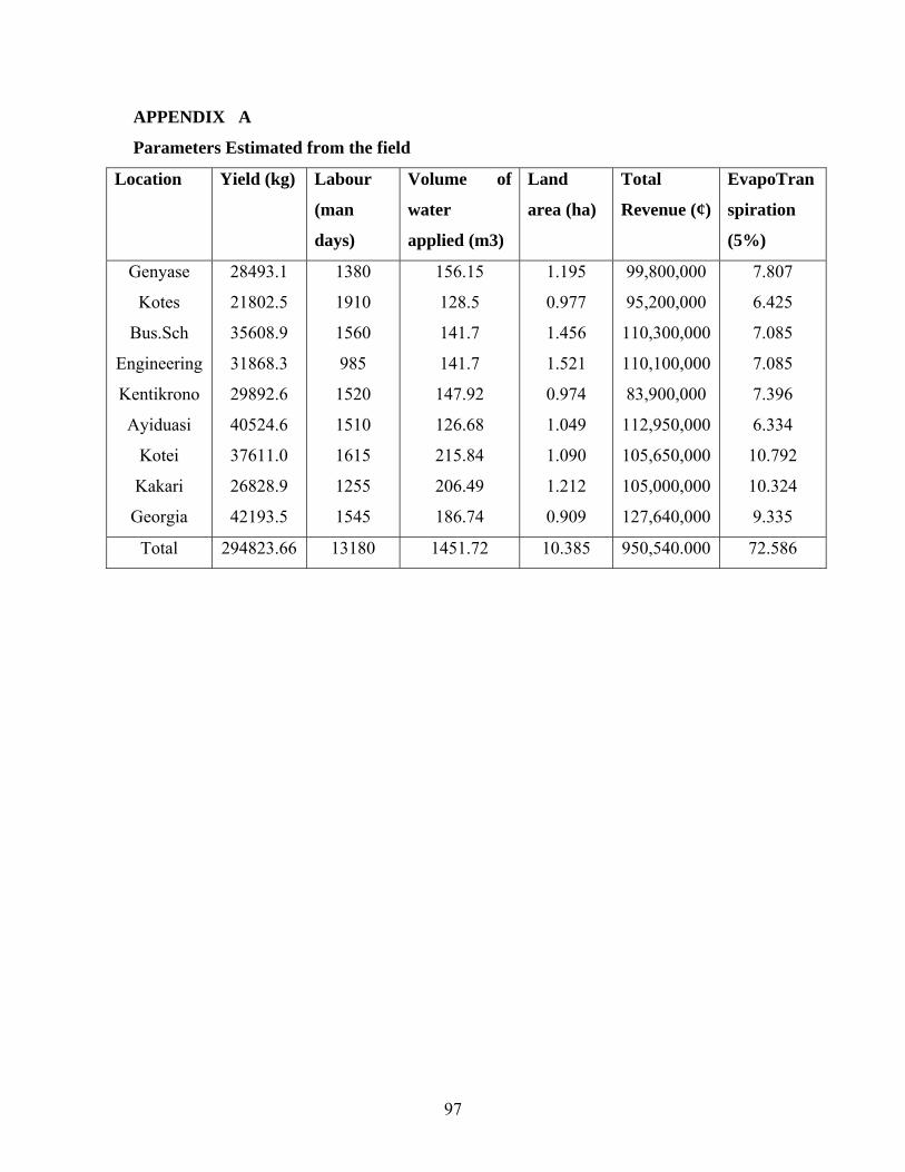
97

APPENDIX A

Parameters Estimated from the field

Location Yield (kg) Labour

(man

days)

Volume of

water

applied (m3)

Land

area (ha)

Total

Revenue (¢)

EvapoTran

spiration

(5%)

Genyase

Kotes

Bus.Sch

Engineering

Kentikrono

Ayiduasi

Kotei

Kakari

Georgia

28493.1

21802.5

35608.9

31868.3

29892.6

40524.6

37611.0

26828.9

42193.5

1380

1910

1560

985

1520

1510

1615

1255

1545

156.15

128.5

141.7

141.7

147.92

126.68

215.84

206.49

186.74

1.195

0.977

1.456

1.521

0.974

1.049

1.090

1.212

0.909

99,800,000

95,200,000

110,300,000

110,100,000

83,900,000

112,950,000

105,650,000

105,000,000

127,640,000

7.807

6.425

7.085

7.085

7.396

6.334

10.792

10.324

9.335

Total 294823.66 13180 1451.72 10.385 950,540.000 72.586

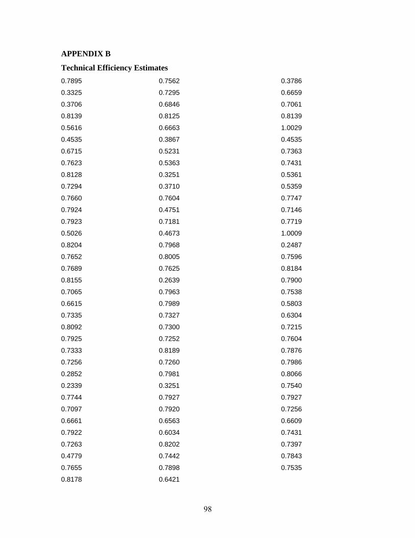
98

APPENDIX B

Technical Efficiency Estimates 0.7895 0.7562 0.3786

0.3325 0.7295 0.6659

0.3706 0.6846 0.7061

0.8139 0.8125 0.8139

0.5616 0.6663 1.0029

0.4535 0.3867 0.4535

0.6715 0.5231 0.7363

0.7623 0.5363 0.7431

0.8128 0.3251 0.5361

0.7294 0.3710 0.5359

0.7660 0.7604 0.7747

0.7924 0.4751 0.7146

0.7923 0.7181 0.7719

0.5026 0.4673 1.0009

0.8204 0.7968 0.2487

0.7652 0.8005 0.7596

0.7689 0.7625 0.8184

0.8155 0.2639 0.7900

0.7065 0.7963 0.7538

0.6615 0.7989 0.5803

0.7335 0.7327 0.6304

0.8092 0.7300 0.7215

0.7925 0.7252 0.7604

0.7333 0.8189 0.7876

0.7256 0.7260 0.7986

0.2852 0.7981 0.8066

0.2339 0.3251 0.7540

0.7744 0.7927 0.7927

0.7097 0.7920 0.7256

0.6661 0.6563 0.6609

0.7922 0.6034 0.7431

0.7263 0.8202 0.7397

0.4779 0.7442 0.7843

0.7655 0.7898 0.7535

0.8178 0.6421

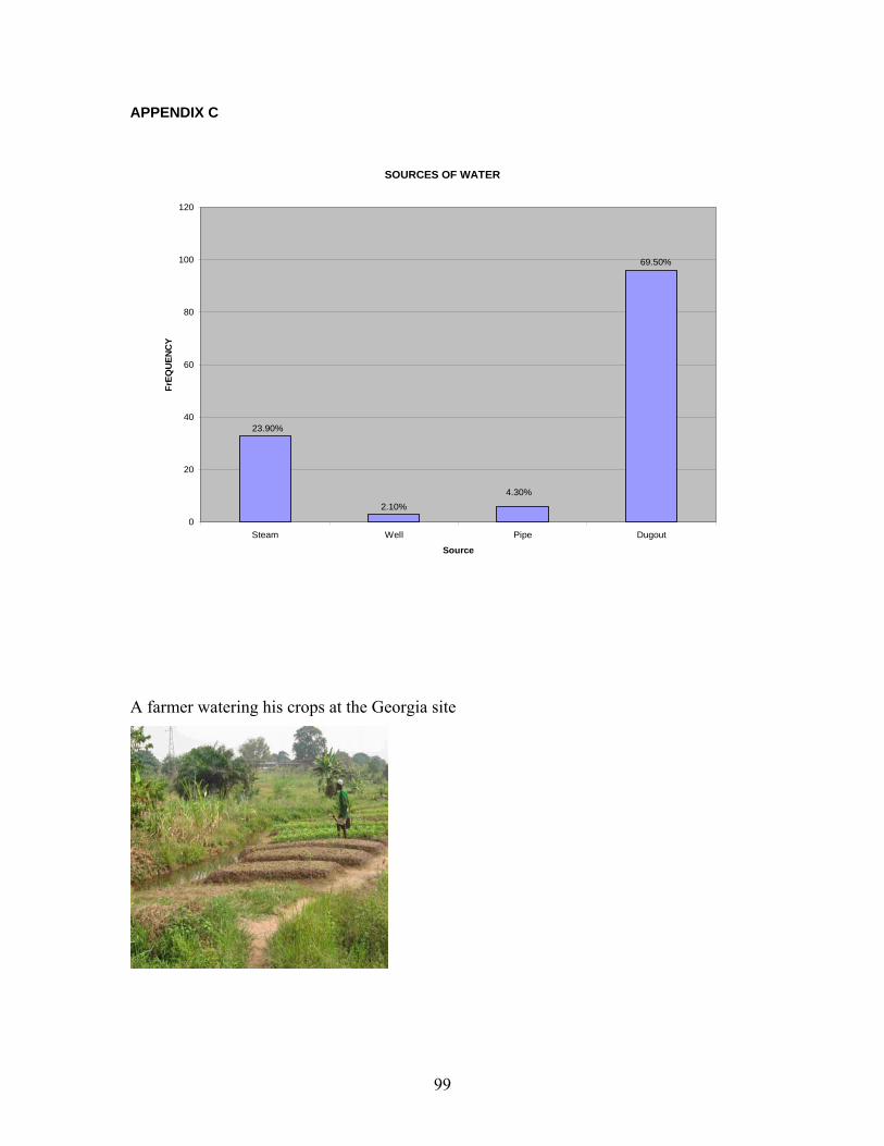
99

APPENDIX C

SOURCES OF WATER

0

20

40

60

80

100

120

Steam Well Pipe Dugout

Source

FrEQ

UEN

CY

23.90%

2.10%4.30%

69.50%

A farmer watering his crops at the Georgia site

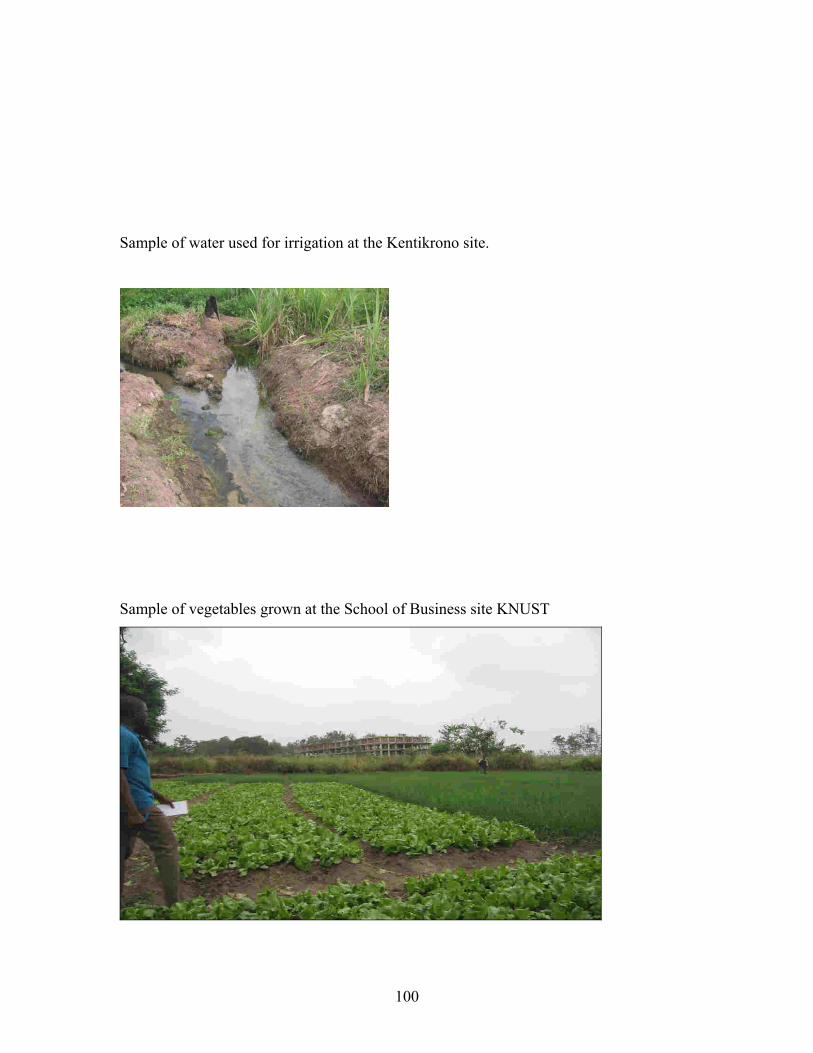
100

Sample of water used for irrigation at the Kentikrono site.

Sample of vegetables grown at the School of Business site KNUST

101

APPENDIX D

RESOURCE USE EFFICIENCY IN VEGETABLE PRODUCTION

FIELD SURVEY QUESTIONNAIRE

BACKGROUND

1 Date…………… 2 Questionnaire number…………………

3 Name of interviewer…………………………………………………..

4 Name of farmer:………………………………………………………

5 Age of respondent:…………… 6. Sex………………………….

7 Location/ Site:……………………………………………………..

8 Marital Status: Married [1] Single [2] Widowed [3]

9 Farmer’s household Size:…………………………………………….

10 Level of respondent’s education:

Illiterate /Basic[1] secondary [2] Tertiary [4]

11 Religion: Christianity [1] Islam [2] others [3]…………

12 What is your main occupation?:…………………………………

Agriculture [1] Trading/Commerce [2] Artisan/Carpentry[3]

public Service [4] Others [5] specify………….

13 How much do you earn on the average per month/season?.......................

14 Apart from farming what other work do you do?

Public Service [1] Trading/Commerce[2] Artisan/Carpentry[3]

Agriculture [4] Others [5] Specify…………………………

15 How much do you earn per month/season?.........................................

16 Since when did you start cultivating vegetables?....................................

LAND TENURE

I How did you get the ownership of this farm? Purchase [1] Rented [4]

inheritance [2] donation [3] Share Cropping [5] others [5]

specify………..

2 If purchased, indicate the Cost of land purchased per

season/year……………………

102

3 If rented, what is the cost ………………… and conditions attached in

using the land per season?...........................................................................

4 What is the total size of your vegetable farm?…………………………

5 What size of the land was used for Lettuce…………… and Cabbage

……….Cultivation this season?

6 Have you increased the area for these two crops this season as compared

to last two years? Yes [1] No [0]

7 If yes, by how much area?....................

8 do you think the acquisition of land is a constraint to vegetable production

in the area? Yes [1] No [0]

LABOUR

1 Source of labour used: Family [1] Hired labour [2]

2 If family labour is used, indicate the number of people who worked

permanently on the field during this season……………….

3 How many man-days do you work on the farm per

week?.................................

4 Complete the table below if hired labour was used.

Farm

Operation

No. of

people

duration of

labor contract

No.of man

days

Wage

Rate/day

Total

Cost

Land clearing

Bed Preparation

Nursery work

Planting

Weeding/fokinSpra

ying

Fert. application

Watering

Harvesting

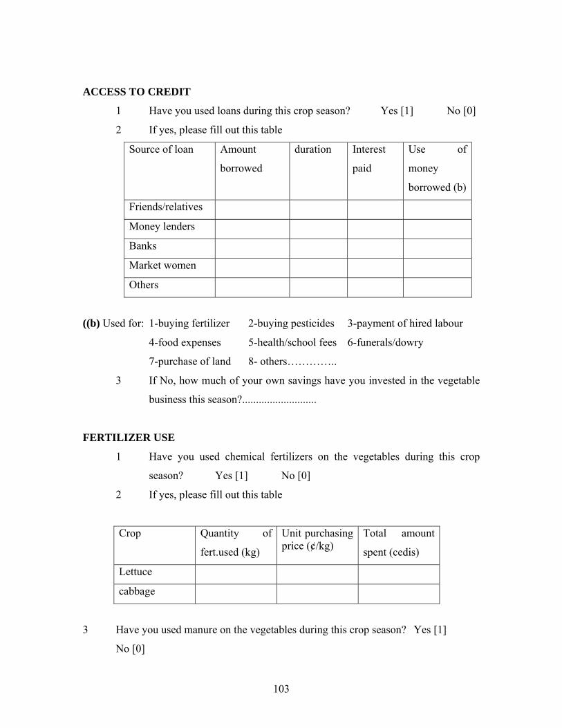
103

ACCESS TO CREDIT

1 Have you used loans during this crop season? Yes [1] No [0]

2 If yes, please fill out this table

Source of loan Amount

borrowed

duration Interest

paid

Use of

money

borrowed (b)

Friends/relatives

Money lenders

Banks

Market women

Others

((b) Used for: 1-buying fertilizer 2-buying pesticides 3-payment of hired labour

4-food expenses 5-health/school fees 6-funerals/dowry

7-purchase of land 8- others…………..

3 If No, how much of your own savings have you invested in the vegetable

business this season?...........................

FERTILIZER USE

1 Have you used chemical fertilizers on the vegetables during this crop

season? Yes [1] No [0]

2 If yes, please fill out this table

Crop Quantity of

fert.used (kg)

Unit purchasing price (¢/kg)

Total amount

spent (cedis)

Lettuce

cabbage

3 Have you used manure on the vegetables during this crop season? Yes [1]

No [0]

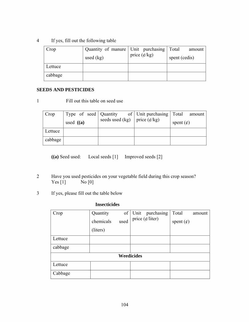
104

4 If yes, fill out the following table

Crop Quantity of manure

used (kg)

Unit purchasing price (¢/kg)

Total amount

spent (cedis)

Lettuce

cabbage

SEEDS AND PESTICIDES 1 Fill out this table on seed use

((a) Seed used: Local seeds [1] Improved seeds [2]

2 Have you used pesticides on your vegetable field during this crop season? Yes [1] No [0] 3 If yes, please fill out the table below Insecticides

Crop Quantity of

chemicals used

(liters)

Unit purchasing price (¢/liter)

Total amount

spent (¢)

Lettuce

cabbage

Weedicides

Lettuce

Cabbage

Crop Type of seed

used ((a)

Quantity of seeds used (kg)

Unit purchasing price (¢/kg)

Total amount

spent (¢)

Lettuce

cabbage

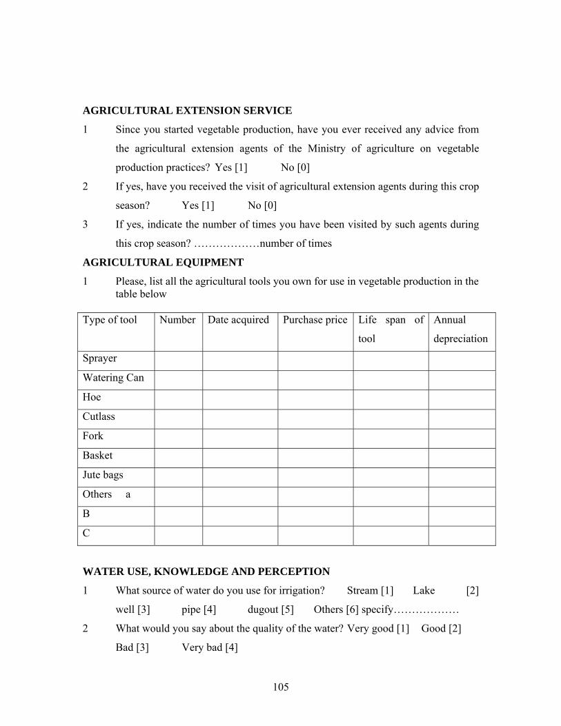
105

AGRICULTURAL EXTENSION SERVICE

1 Since you started vegetable production, have you ever received any advice from

the agricultural extension agents of the Ministry of agriculture on vegetable

production practices? Yes [1] No [0]

2 If yes, have you received the visit of agricultural extension agents during this crop

season? Yes [1] No [0]

3 If yes, indicate the number of times you have been visited by such agents during

this crop season? ………………number of times

AGRICULTURAL EQUIPMENT

1 Please, list all the agricultural tools you own for use in vegetable production in the table below

Type of tool Number Date acquired Purchase price Life span of

tool

Annual

depreciation

Sprayer

Watering Can

Hoe

Cutlass

Fork

Basket

Jute bags

Others a

B

C

WATER USE, KNOWLEDGE AND PERCEPTION

1 What source of water do you use for irrigation? Stream [1] Lake [2]

well [3] pipe [4] dugout [5] Others [6] specify………………

2 What would you say about the quality of the water? Very good [1] Good [2]

Bad [3] Very bad [4]

106

3 Do you drink the water you use for irrigation? Yes [1] No [0]

4 If no, why?..............................................................................................................

5 Do you experience any health problems in using the water for irrigation?

Yes [1] No [0]

6 If yes, what are they?…………………………………………………………….. ………………………………………………………………………………………………………………………………

7 Has any customer ever complained of any health problems after consuming

vegetables produced by you? Yes [1] No [0]

8 If yes, what was the problem ………………………………….and what was your

Response?.................................................................................................................

9 Do you pay for the water you use for irrigation? Yes [1] No [0]

10 If yes, how much per month?……………………………………………………

11 If there is an option {pipe water} to the water being used currently, would you be

willing to pay some amount for it? Yes [1] No [0]

12 What quantity of water (in Cans) do you usually apply per day on

cabbage……………… and lettuce……………….per bed?

13 How often do you water the plants? Once a day [1] Twice a day [2]

Once every two days [3] Once every three days [4] Other [5]……..

OUTPUT AND MARKETING

1 Please indicate the quantities of vegetables harvested this season from your field.

Crop Quantity harvested(kg) /No. of beds *No of plants

Lettuce

cabbage

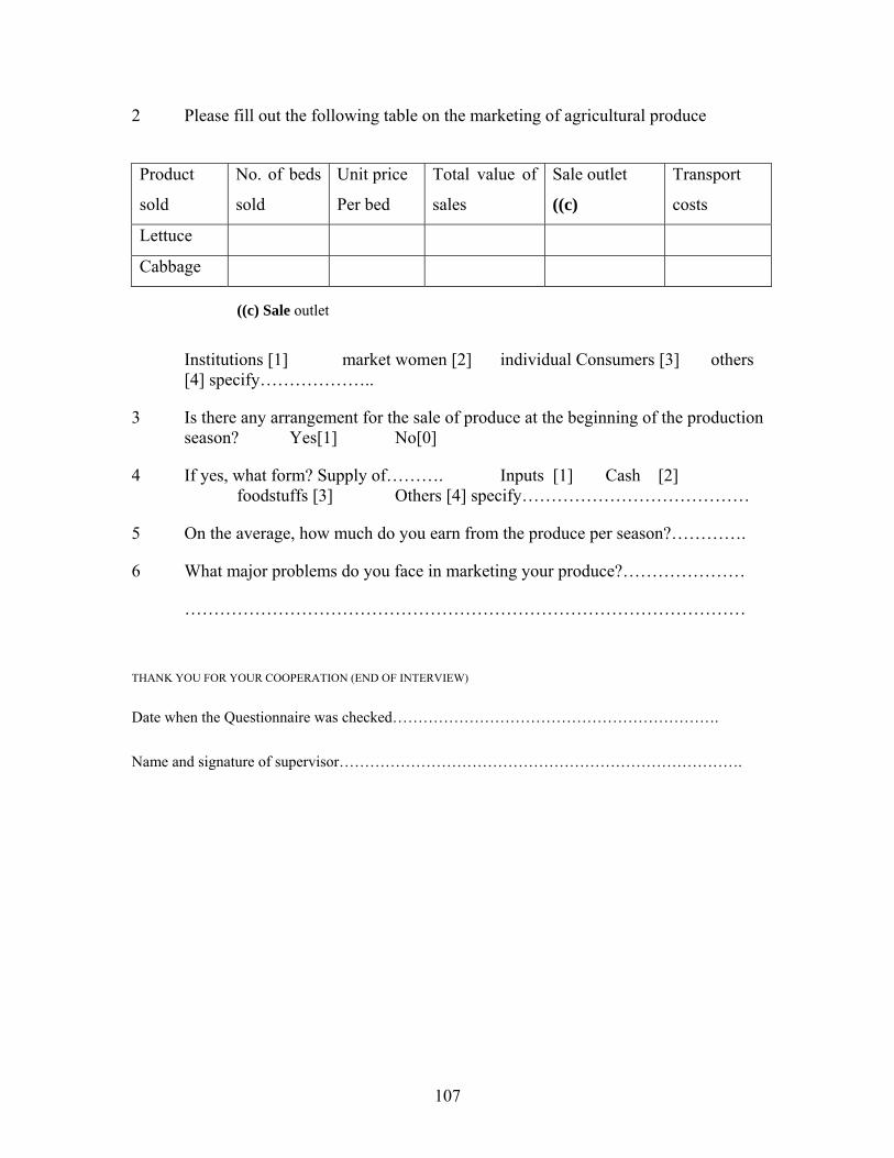
107

2 Please fill out the following table on the marketing of agricultural produce

Product

sold

No. of beds

sold

Unit price

Per bed

Total value of

sales

Sale outlet

((c)

Transport

costs

Lettuce

Cabbage

((c) Sale outlet

Institutions [1] market women [2] individual Consumers [3] others [4] specify………………..

3 Is there any arrangement for the sale of produce at the beginning of the production season? Yes[1] No[0]

4 If yes, what form? Supply of………. Inputs [1] Cash [2] foodstuffs [3] Others [4] specify…………………………………

5 On the average, how much do you earn from the produce per season?………….

6 What major problems do you face in marketing your produce?…………………

……………………………………………………………………………………

THANK YOU FOR YOUR COOPERATION (END OF INTERVIEW)

Date when the Questionnaire was checked……………………………………………………….

Name and signature of supervisor…………………………………………………………………….