Resource Bricolage for Parallel Database Systems

Jiexing Li #, Jeffrey Naughton #, Rimma V. Nehme ∗

#University of Wisconsin, Madison ∗Microsoft Jim Gray Systems Lab{jxli, naughton}@cs.wisc.edu rimman@microsoft.com

ABSTRACTRunning parallel database systems in an environment withheterogeneous resources has become increasingly common,due to cluster evolution and increasing interest in movingapplications into public clouds. For database systems run-ning in a heterogeneous cluster, the default uniform datapartitioning strategy may overload some of the slow ma-chines while at the same time it may under-utilize the morepowerful machines. Since the processing time of a parallelquery is determined by the slowest machine, such an alloca-tion strategy may result in a significant query performancedegradation.

We take a first step to address this problem by intro-ducing a technique we call resource bricolage that improvesdatabase performance in heterogeneous environments. Ourapproach quantifies the performance differences among ma-chines with various resources as they process workloads withdiverse resource requirements. We formalize the problem ofminimizing workload execution time and view it as an opti-mization problem, and then we employ linear programmingto obtain a recommended data partitioning scheme. Weverify the effectiveness of our technique with an extensiveexperimental study on a commercial database system.

1. INTRODUCTIONWith the growth of the Internet, our ability to generate

extremely large amounts of data has dramatically increased.This sheer volume of data that needs to be managed andanalyzed has led to the wide adoption of parallel databasesystems. To exploit data parallelism, these systems typicallypartition data among multiple machines. A query runningon the systems is then broken up into subqueries, which areexecuted in parallel on the separate data chunks.

Nowadays, running parallel database systems in an envi-ronment with heterogeneous resources has become increas-ingly common, due to cluster evolution and increasing inter-est in moving applications into public clouds. For example,when a cluster is first built, it typically begins with a set

This work is licensed under the Creative Commons Attribution-NonCommercial-NoDerivs 3.0 Unported License. To view a copy of this li-cense, visit http://creativecommons.org/licenses/by-nc-nd/3.0/. Obtain per-mission prior to any use beyond those covered by the license. Contactcopyright holder by emailing info@vldb.org. Articles from this volumewere invited to present their results at the 41st International Conference onVery Large Data Bases, August 31st - September 4th 2015, Kohala Coast,Hawaii.Proceedings of the VLDB Endowment, Vol. 8, No. 1Copyright 2014 VLDB Endowment 2150-8097/14/09.

0

100

200

300

400

Q1 Q2 Q3 Q4 Q5

TPC-H Query

Query execution time (sec)

UniformBricolage

Figure 1: Query execution times with different datapartitioning strategies.

of identical machines. Over time, old machines may be re-configured, upgraded, or replaced, and new machines maybe added, thus resulting in a heterogeneous cluster. At thesame time, more and more parallel database systems aremoving into public clouds. Previous research has revealedthat the supposedly identical instances provided by publicclouds often exhibit measurably different performance. Per-formance variations exist extensively in disk, CPU, memory,and network [12, 20, 29, 30].

1.1 MotivationPerformance differences among machines (either physi-

cal or virtual) in the same cluster pose new challenges forparallel database systems. By default, parallel systems ig-nore differences among machines and try to assign the sameamount of data to each. If these machines have differentdisk, CPU, memory, and network resources, they will takevarying amounts of time to process the same amount of data.Unfortunately, the execution time of a query in a paralleldatabase system is determined by its slowest machine. Atworst, a slow machine can substantially degrade the perfor-mance of the query.

On the other hand, a fast machine in such a system willbe under-utilized, finishing its work early, sitting idle, andwaiting for the slower machines to finish. This suggests thatwe can reduce execution time by allocating more data tomore powerful machines and less data to the overloaded slowmachines, in order to reduce the execution times of the slowones. In Figure 1, we compare the execution times of thefirst 5 TPC-H queries running on a heterogeneous clusterwith two different data partitioning strategies. One strategypartitions the data uniformly across all the machines, whilethe other partitions the data using our proposed technique,which we present in Section 4. The detailed cluster setupis described in Section 5. As can be seen from the graph,we can significantly reduce total query execution time by

25

carefully partitioning the data.Our task is complicated by the fact that whether a ma-

chine should be considered powerful or not depends on theworkload. For example, a machine with powerful CPUs isconsidered “fast” if we have a CPU-intensive workload. Foran I/O-intensive workload, it is considered “slow” if it haslimited disks. Furthermore, to partition the data in a betterway, we also need to know how much data we should allocateper machine. Obviously, enough data should be assigned tomachines to fully exploit their potential for the best perfor-mance, but at the same time, we do not want to push toofar to turn things around by overloading the powerful ma-chines. The problem gets more complicated when queries ina workload have different (mixed) resource requirements, asusually happens in practice. For a workload with a mix ofI/O, CPU, and network-intensive queries, the partitioningof data with the goal of reducing overall execution time is anon-trivial task.

Automated partitioning design for parallel databases isa fairly well-researched problem [8, 25, 26, 27]. The pro-posed approaches improve system performance by selectingthe most suitable partitioning keys for base tables or min-imizing the number of distributed transactions for OLTPworkloads. Somewhat surprisingly, despite the apparent im-portance of this problem, no existing approach aims directlyat minimizing decision support execution time for hetero-geneous clusters. We will provide detailed explanations inSection 6.

1.2 Our ContributionsTo improve performance of parallel database systems run-

ning in heterogeneous environments, we propose a techniquewe call resource bricolage. The term bricolage refers toconstruction or creation of a work from a diverse range ofthings that happen to be available, or a work created by sucha process. The keys to the success of bricolage are knowingthe characteristics of the available items, and knowing a wayto utilize and get the most out of them during construction.

In the context of our problem, a set of heterogeneous ma-chines are the available resources, and we want to use themto process a database workload as fast as possible. Thus,to implement resource bricolage, we must know the perfor-mance characteristics of the machines that execute databasequeries, and we must also know which machines to use andhow to partition data across them to minimize workloadexecution time. To do this, we quantify differences amongmachines by using the query optimizer and a set of profilingqueries that estimate the machines’ performance parame-ters. We then formalize the problem of minimizing work-load execution time and view it as an optimization prob-lem that takes the performance parameters as input. Wesolve the problem using a standard linear program solver toobtain a recommended data partitioning scheme. In Sec-tion 4.4, we also discuss alternatives for handling nonlinearsituations. We implemented our techniques and tested themin Microsoft SQL Server Parallel Data Warehouse (PDW)[1], and our experimental results show the effectiveness ofour proposed solution.

The rest of the paper is organized as follows. Section 2 for-malizes the resource bricolage problem. Section 3 describesour way of characterizing the performance of a machine.Section 4 presents our approach for finding an effective datapartitioning scheme. Section 5 experimentally confirms the

effectiveness of our proposed solution. Section 6 briefly re-views the related work. Finally, Section 7 concludes thepaper with directions for future work.

2. THE PROBLEM

2.1 FormalizationTo enable parallelism in a parallel database system, ta-

bles are typically horizontally partitioned across machines.The tuples of a table are assigned to a machine either byapplying a partitioning function, such as a hash or a rangepartitioning function, or in a round-robin fashion. A par-titioning function maps the tuples of a table to machinesbased on the values of specified column(s), which is (are)called the partitioning key of the table. As a result, a par-titioning function determines the number of tuples that willbe mapped to each machine.

CPU

DiskDiskDisk

CPU CPU

Partitioning schemes

For I/O-intensive queries:

For CPU-intensive queries:

33% 67%

67% 33%

Machine 1 Machine 2

Figure 2: Different data partitioning schemes.

A uniform partitioning function may result in poor per-formance. Let us consider a simple example where we havetwo machines in a cluster as shown in Figure 2. Let theCPUs of the first machine be twice as fast as that of thesecond machine, and let the disks of the first machine be50% slower than that of the second machine. We want tofind the best data partitioning scheme to allocate the datato these two machines. Suppose that we have only one queryin our workload, and it is I/O intensive. This query scansa table and counts the number of tuples in the table. Thequery completes when both machines finish their process-ing. To minimize the total execution time, it is easy forus to come up with the best partitioning scheme, which as-signs 33% of the data to the first machine and 67% of thedata to the second machine. In this case, both machineswill have similar response times. Assume now that we adda CPU-intensive query to the workload. It scans and sortsthe tuples in the table. Determining the best partitioningscheme in this case becomes a non-trivial task. Intuitively,if the CPU-intensive query takes longer to execute than theI/O-intensive query, we should assign more data to the firstmachine to take advantage of its more powerful CPUs, andvice versa.

...Workload

Query 1

Query q

...

Step 1

Step s

(Subquery 1, …, Subquery n)

...

...

Figure 3: A query workload.

In general, we may have a set of heterogeneous machineswith different disk, CPU, and network performance, andthey may have different amounts of memory. At the sametime, we have a workload with a set of SQL queries as shown

26

in Figure 3. A query can be further decomposed into a num-ber of steps with different resource requirements. For eachstep, there will be a set of identical subqueries executing con-currently on different machines to exploit data parallelism.A step will not start until all steps upon which it dependson, if any, have finished. Thus, the running time of a stepis determined by the longest-running subquery. The queryresult of a step will be repartitioned to be utilized by latersteps, if needed.

t11

M1

t21 tn1...

t12 t22 tn2...

t1h t2h tnh...

...

M2 Mn

S1

S2

Sh

n machines

h steps

l1 l2 ln

Figure 4: Problem setting.

We visually depict our problem setting in Figure 4. LetM1, M2, ..., Mn be a set of machines in the cluster, and letW be a workload consisting of multiple queries. Each queryconsists of a certain number of steps, and we concatenate allthe steps in all of the queries to get a total of h steps: S1,S2, ..., Sh. Assume that tij would be the execution time forstep Sj running on machine Mi if all the data were assignedto Mi. Each column in the graph corresponds to a machine,and each row represents the set of subqueries running on themachines for a particular step. In addition, we assume thata machine Mi also has a storage limit li, which representsthe maximum percentage of the entire data set that it canhold. The goal of resource bricolage is to find the best wayto partition data across machines in order to minimize thetotal execution time of the entire workload.

2.2 Potential for ImprovementWhether it is worth allocating data to machines in a non-

uniform fashion is dependent on the characteristics of theavailable computing resources. If all the machines in a clus-ter are identical or have similar performance, there is no needfor us to consider the resource bricolage problem at all. Atthe other extreme, if all the machines are fast except for afew slow ones, we can improve performance and come closeto the optimal solution by just deleting the slow machines.The time that we can save by dealing with performancevariability depends on many factors, such as the hardwaredifferences among machines, the percentage of fast/slow ma-chines, and the workloads.

To gain preliminary insight as to when explicitly modelingresource heterogeneity can and cannot pay off, we considerthree data partitioning strategies: Uniform, Delete, and Op-timal. Uniform is the default data allocation strategy of aparallel database system. It ignores differences among ma-chines and assigns the same amount of data to each ma-chine. Since there is no commonly accepted approach forthe problem we address in the paper, we propose Delete asa simple heuristic that attempts to handle resource hetero-geneity. It deletes some slow machines before it partitionsthe data uniformly to the remaining ones. It tries to deletethe slowest set of machines first, and then the second slowest

next. This process is repeated until no further improvementcan be made. Optimal is the ideal data partitioning strategythat we want to pursue. It distributes data to machines in away that can minimize the overall workload execution time.The corresponding query execution times for these strategiesare denoted as tu, tdel, and topt, respectively. According tothe definitions, we have tu ≥ tdel ≥ topt.

We start with a simple case with n machines in total,where a fraction p of them are fast and (1−p) are slow. Ourworkload contains just one single-step query. For simplicity,we assume that one fast machine can process all data in 1unit of time (e.g., 1 hour, 1 day, etc.), and the slow machinesneed r units of time (r ≥ 1). We also assume that, for eachmachine, the processing time of a step changes linearly withthe amount of data. The value r can also be consideredto be the ratio between execution times of a slow machineand a fast machine. We omit the underlying reasons thatlead to the performance differences (e.g., due to a slow disk,CPU, or network connection), since they are not importantfor our discussion here. It is easy to see that tu = 1

nr,

tdel = min{ 1nr, 1

np}. In this limited specialized case that we

are considering, calculating topt is easy and can be conductedin the following way. We denote the fractions of data weallocate to a fast machine as p1 and to a slow machine as p2,respectively. The optimal strategy assigns data to machinesin such a way that the processing times are identical. Thiscan be represented as p1 = rp2. Since the sum of p1 and p2is 1, we can derive topt = r

n(rp+1−p).

To see how much improvement we can make by goingfrom a simple strategy to a more sophisticated one, we cal-culate the percentage of time we can reduce from t1 to t2 as100(1− t2/t1). We discuss the reduction that can be madeby adopting the simple heuristic Delete first, and then wepresent the further reduction that can be achieved by tryingto come up with Optimal.

From Uniform to Delete. When r ≤ 1p, we have tdel =

1nr = tu. The decision is to keep all machines, and no

improvement can be made by deleting slow machines. Whenr > 1

p, tdel = 1

np. The percentage of reduction we can make

is 100(1− 1rp

). When rp is big, the percentage of reduction

can get close to 100%. Delete is well-suited for clusters wherethere are only a few slow machines and the more powerfulmachines are much faster than the slow ones. Thus, given aheterogeneous cluster, the first thing we should do is try tofind the slow outliers and delete them.

0 20 40 60 80 1005

1015

200

1020304050

Percent of improvement (%)

p% of fast machines

Ratio r

Percent of improvement (%)

Figure 5: Potential for improvement.

From Delete to Optimal. In this case, the improve-ment we can make is not so obvious. In Figure 5, we plot thepercentage of time that can be reduced from tdel to topt. Wevary p from 0 to 100% and r from 0 to 20. As we can see fromthe graph, when r is fixed, the percentage of reduction in-creases at first and then decreases as p gets bigger. Similarly,

27

when p is fixed, the percentage of reduction also increases atfirst and then decreases as we vary r from 0 to 20. More pre-cisely, when r ≤ 1

p, tdel = 1

nr. The percentage of reduction

can be calculated as 100(1 − topt/tdel) = 100(1 − 1rp+1−p

).Since rp ≤ 1, we have rp + 1 − p < 2. As a result, the re-duction 100(1− 1

rp+1−p) is less than 50%. When r > 1

p, we

have tdel = 1np

, and the reduction is 100(1− 1

1+ 1rp

− 1r

). Since

rp > 1, the denominator is no larger than 2. Therefore, thepercent of reduction is also less than 50%.

Now, let us consider a more complicated example with nmachines and n/2 + 1 steps. In this example, we will showthat in the worst case, the performance gap between Deleteand Optimal can be arbitrarily large. The detailed tij valuesare indicated in Figure 6, where a is large constant and εis a very small positive number. If we use each machine in-dividually to process the data, the workload execution timefor a machine in the first half on the left is a+(n

2+1)ε. This

is longer than the workload execution time a + (n2− 1)ε for

a machine in the second half. When we look at these ma-chines individually, the first n/2 of them are considered tobe relatively slow.

M1 Mn/2 Mn/2+2

S1

Mn/2+1

S2

S3

a+ɛ

ɛ

ɛ

a+ɛ

ɛ

ɛ

ɛ

a-ɛ

ɛ

ɛ

ɛ

a-ɛ...

Mn

ɛ

ɛ

ɛ

Sn/2+1 ɛ ɛ ɛ ɛ a-ɛ

...

“slow” machines “fast” machines

Figure 6: A worst-case example.

Given these machines, Delete works as follows. First, itcalculates the execution time of the workload when data ispartitioned uniformly across all machines. The runtime forthe first step S1 is 1

n(a+ ε). The runtime for a later step Sj

(j ≥ 2) is 1n

(a− ε), which is the processing time of machineMn/2+j−1. In total, we have n/2 number of such steps. Asa result, the execution time of all steps is 1

n(a+ε)+ 1

2(a−ε).

Then Delete tries to reduce the execution time by deletingslow machines, thus it will try to delete {M1, M2, ..., Mn/2}first. We can prove that the best choice for Delete is to useall machines. On the other hand, the optimal strategy isto use just the “slow” machines and assign 2

nof the data

to each of them, and we have topt = 2n

(a + ε). AlthoughDelete uses more machines than Optimal, it is easy to getthat tdel

topt≈ n

4.

2.3 ChallengesAlthough the worst-case situation may not happen very

often in the real world, our main point here is that whenthere are many different machines in a cluster and we havequeries with various resource demands, the heuristic (Delete)that works well for simple cases may generate results farfrom optimal. In addition, the heuristic works by deletingthe set of obviously slow machines. However, simple caseswhere we can divide machines in the same cluster into a fastgroup and a slow group may not happen very often. Accord-ing to Moore’s law, computers’ capabilities double approx-imately every two years. If cluster administrators performhardware upgrades every one or two years, it is reasonableto assume that we may see 2x, 4x, or maybe 8x differences inmachine performance in the same cluster. This assumption

is also consistent with what has been observed in a very largeGoogle cluster [28]. Normally, we would not add a machineto a cluster that is significantly different from the others toperform the same tasks. On the other hand, machines thatare too slow and out of date will be eventually phased out.For systems running on a public cloud, requesting a set ofVM instances of the same type to run an application is themost common situation. As we discussed in Section 1, thesupposedly identical instances from public clouds may stillhave different performance. Previous studies, which used anumber of benchmarks to test the performance of 40 Ama-zon EC2 m1.small instances, observed that the speedup ofthe best performance instance over the worst performanceinstance is usually in the range from 0% to 300% for differentresources [12].

Thus, it is important for us to come up with the optimalpartitioning strategy to better utilize computing resources.To do this, there are a number of challenges that need to betackled. First of all, we need to quantify performance differ-ences among machines in order to assign the proper amountsof data to them. Second, we need to know which machinesto use and how much data to assign to each of them forbest performance. Intuitively, we should choose “fast” ma-chines, and we should add more machines to a cluster toreduce query execution times. However, this is not true inthe worst-case example we discussed. In our example, theperformance of the set of “slow” machines used by Optimalare similar, and the bottlenecks of the subqueries are clus-tered on the same step (S1). Delete uses some additional“fast” machines, but these machines do not collaborate wellin the system. They introduce additional bottlenecks inother steps (S2 to Sn/2+1), which result in longer executiontimes.

3. QUANTIFYING PERFORMANCEDIFFERENCES

For each machine in the cluster, we use the runtimes ofthe queries that will be executed to quantify its performance.Since we do not know actual query execution times beforethey finish, we need to estimate these values.

There has been a lot of work in the area of query execu-tion time estimation [5, 6, 16, 18, 23]. Unlike previous work,we do not need to get perfect time estimates to make a gooddata partitioning recommendation. As we will see in the ex-perimental section, the ratios in time between machines arethe key information that we need to deal with heterogeneousresources. Thus, we adopt a less accurate but much simplerapproach to estimate query execution times. Our approachcan be summarized as follows. For a given database query,we retrieve its execution plan from the optimizer, and wedivide the plan into a set of pipelines. We then use the opti-mizer’s cost model to estimate the CPU, I/O, and network“work” that needs to be done by each pipeline. To estimatethe times to execute the pipelines on different machines, werun profiling queries to measure the speeds to process theestimated work for each machine.

3.1 Estimating the Cost of a PipelineLike previous work on execution time estimation [6, 18],

we use the execution plan for a query to estimate its runtime.An execution plan is a tree of physical operators chosen bya query optimizer. In addition to the most commonly used

28

operators in a single-node DBMS, such as Table Scan, Filter,Hash Join, etc., a parallel database system also employs datamovement operators, which are used for transferring databetween DBMS instances running on different machines.

Table Scan

[Orders]

Hash Join

Table Scan

[Lineitem]

Shuffle Move

[Temp t]

P1

P2

Figure 7: An execution plan with two pipelines.

An execution plan is divided into a set of pipelines delim-ited by blocking operators (e.g., Hash Join, Group-by, anddata movement operators). The example plan in Figure 7 isdivided into two different pipelines P1 and P2. Pipelines areexecuted one after another. If we can estimate the executiontime for each pipeline, the total runtime of a query is sim-ply the sum of the execution time(s) of its pipeline(s). Toestimate a pipeline’s execution time, we first predict whatis the work of the pipeline and what is the speed to processthe work. We then estimate the runtime of a pipeline as theestimated work divided by the processing speed.

For each pipeline, we use the optimizer’s cost model toestimate the work (called cost) that needs to be done byCPUs, disks, and network, respectively. These costs areestimated based on the available memory size. We utilizethe optimizer estimated cost units to define the work for anoperator in a pipeline. We follow the idea presented in [16]to calculate the cost for a pipeline, and the interested readeris referred to that paper for details.

However, the default optimizer estimated cost is calcu-lated using parameters with predefined values (e.g., the timeto fetch a page sequentially), which are set by optimizer de-signers without taking into account the resources that willbe available on the machine for running a query. Thus, itis not a good indication of actual query execution time fora specific machine. To obtain more accurate predictions,we keep the original estimates and treat them as estimatedwork if a query was to run on a “standard” machine withdefault parameters. Then, we test on a given machine tosee how fast it can go through this estimated work with itsresources (the speeds).

3.2 Measuring Speeds to Process the CostMeasuring I/O speed. To test the speed to process the

estimated I/O cost for a machine, we execute the followingquery with a cold buffer cache: select count(*) from T. Thisquery simply scans a table T and returns the number oftuples in the table. It is an I/O-intensive query with negli-gible CPU cost. For this query, we use the query optimizerto get its estimated I/O cost, and then we run it to obtainits execution time for the given machine. Then we calculatethe I/O speed for this machine as the estimated I/O costdivided by the query execution time.

Measuring CPU speed. To measure the CPU speed,we test a CPU-intensive query: select T.a from T group byT.a from a warm buffer cache. For this query, we can alsoget its estimated CPU cost and runtime, and we calculatethe CPU speed for this machine in a similar way. Since small

queries tend to have higher variation in the cost estimatesand execution times, one practical suggestion is to use asufficiently big table for the test. Meanwhile, since the timespent on transferring query results from a database engine toan external test program is not used to process the estimatedCPU cost, we need to limit the number of tuples that willbe returned. In our experiment, T contains 18M unsortedtuples, and only 4 distinct T.a values are returned.

Measuring network speed. We use a small and sepa-rate program to test the network speed instead of a queryrunning on an actual database system. The reason is thatit is hard to find a query to test the network speed whenisolating all other factors that can contribute to query exe-cution times. For a query with data movement operators ina fully functional system, the query may need to read datafrom a local disk and store data in a destination table. Ifnetwork is not the bottleneck resource, we can not observethe true network speed. Thus we wrote a small program toresemble the actual system for transmitting data betweenmachines. We run this program at its full speed to send(receive) data to (from) another machine that is known tohave a fast network connection. At the end, we calculatethe average bytes of data that can be transferred per secondas the network speed for the tested machine.

Finally, for a pipeline P , we estimate its execution time asthe maximum of CRes(P )/SpeedRes, for any Res in {CPU,I/O, network}. The execution time of a plan is the sum ofthe execution times of all pipelines in the plan.

4. RESOURCE BRICOLAGEAfter we estimate the performance differences among ma-

chines for running our workload, we now need to find a bet-ter way to utilize the machines to process a given workloadas fast as possible. We model and solve this problem us-ing linear programming, and we deploy special strategies tohandle nonlinear scenarios.

4.1 Base and Intermediate Data PartitioningData partitioning can happen in two different places. One

is base table partitioning when loading data into a system,and the other one is intermediate result reshuffling at the endof an intermediate step. For example, consider a subquery ofa step that uses the execution plan shown in Figure 7. Thisplan scans two base tables: Lineitem and Orders, which maybe partitioned across all machines. The result of this sub-query, which can be viewed as a temporary table, is servedas input to next steps, if there are any. Thus, the outputtable may also be redistributed among the machines.

The execution time of a plan running on a given machineis usually determined by the input table sizes. For example,the runtime of the plan in Figure 7 depends on the numberof Lineitem and Orders (L and O for short) tuples. Theruntime of a plan that takes a temporary table as input isagain determined by the size of the temporary table.

In some cases, the partitioning of an immediate table canbe independent of the partitioning of any other tables. Forexample, if the output of L ./ O is used to perform a lo-cal aggregate in the next step, we can use a partitioningfunction different from the one used to partition L and Oto redistribute the join results. However, if the output ofL ./ O is used to join with other tables in a later step,we must partition all tables participating in the join in adistribution-compatible way. In other words, we have to use

29

the same partitioning function to allocate the data for thesetables.

In our work, we consider data partitioning for both baseand intermediate tables. Note that our technique can alsobe applied to systems that do not partition base tables apriori or do not store data in local disks. For these systems,our approach can be used to decide the initial assignmentof data to the set of parallel tasks running with heteroge-neous resources, and similarly, our approach can be usedfor intermediate result reshuffling. Instead of reading pre-partitioned data from local disks, these systems read datafrom distributed file systems or remote servers. In order toapply our technique, we need to replace the time estimatesfor reading data locally with the time estimates for access-ing remote data. We omit the details here since it is not thefocus of our paper.

4.2 The Linear Programming ModelNext, we will first give our solution to the situation where

all tables must be partitioned using the same partitioningfunction, and then we extend it to cases where multiple par-titioning functions are allowed at the same time.

Recall that in our problem setting, we have n machines,and the maximum percentage of the entire data set thatmachine Mi can hold is li. Our workload consists of h steps,and it would take time tij for machine Mi to process stepSj if all data were assigned to Mi. The actual tij values areunknown, and we use the technique proposed in Section 3 toestimate them. We want to find a data partitioning schemethat can minimize the overall workload execution time.

When all tables are partitioned in the same way, we canuse just one variable to represent the percentage of data thatgoes to a particular machine for different tables. Let pi bethe percentage of the data that is allocated to Mi for eachtable. We assume that the time it takes for Mi to processstep Sj is proportional to the percentage of data assignedto it. Based on this assumption, pitij represents the time toprocess pi of the data for step Sj running on machine Mi.The execution time of Sj , which is determined by the slow-est machine, is maxn

i=1 pitij . Then the total execution time

of the workload can be calculated as∑h

j=1 maxni=1 pitij . In

order to use a linear program to model this problem, we in-troduce an additional variable xj to represent the executiontime of step Sj . Thus, the total execution time of the work-

load can also be represented as∑h

j=1 xj . The linear programthat minimizes the total execution time of the workload canbe formulated below.

For step Sj , since the execution time xj is the longestexecution time of all machines, we must have pitij ≤ xj formachine Mi. We also know that the percentage of data thatcan be allocated to Mi must be at least 0 and at most li. Thesum of all pis is 1, since all data must be processed. We cansolve this linear programming model using standard linearoptimization techniques to derive the values for pis (0 ≤ i ≤n) and xjs (0 ≤ j ≤ h), where the set of pi values represents

a data partitioning scheme that minimizes∑h

j=1 xj . Notethat we may use only a subset of the machines, since we donot need to run queries on a machine with 0% of the data.Thus, the data partitioning scheme suggests a way to selectthe most suitable set of machines and a way to utilize themto process the database workload efficiently.

4.3 Allowing Multiple Partitioning Functions

minimize

h∑j=1

xj

subject to pitij ≤ xj 1 ≤ i ≤ n, 1 ≤ j ≤ hn∑

i=1

pi = 1

0 ≤ pi ≤ li 1 ≤ i ≤ n

When different partitioning functions are allowed to beused by different tables, we are given more flexibility formaking improvements. Thus, we want to apply differentpartitioning functions whenever possible. In order to do this,we need to identify sets of tables that must be partitioned inthe same way to produce join-compatible distributions, andwe apply different partition functions to tables in differentsets.

Step S

To

Ti1 Ti2 TiI...

Figure 8: The input and output tables for a step.

For step S in workload W , let {Ti1, Ti2, ..., TiI} be theset of its input tables and To be its output table as we showin Figure 8. An input table to S could be a base table oran output table of another step, and all input tables will bejoined together in step S. In order to perform joins, tuplesin these tables must be mapped to machines using the samepartitioning function, otherwise tuples that can be joinedtogether may go to different machines1.

We define a distribution-compatible group as the setof input and output tables for W that must be partitionedusing the same function, together with the set of steps in Wthat take these tables as input. Placing a step to a groupimplies that how to partition the tables in the group hasa significant impact on the execution time of the step. Ifwe can find all distribution-compatible groups for W , wecan apply different functions to tables in different groupsfor data allocation.

Given a database, we assume that the partitioning keysfor base tables and whether two base tables should be parti-tioned in a distribution-compatible way or not are designedby a database administrator or an automated algorithm [2,25, 27]. As a result, we know which base tables shouldbelong to a distribution-compatible group. For interme-diate tables, we need to figure this out. We generate thedistribution-compatible groups for a workload W in the fol-lowing way:

1. Create initial groups with corresponding distribution-compatible base tables according to the database de-sign.

2. For each step S in W , perform the following threeinstructions.

1We omit replicated tables in our problem. Since a full copyof a replicated table will be kept on a machine, there is noneed to worry about partitioning.

30

(a) For the input tables to S, find the groups thatthey belong to. If more than one group is found,we merge them into a single group.

(b) Assign S to the group.

(c) Create a new group with the output table of S.

S1

G1

O → To1

L, O

L, OS1

L, OS1

L, OS1

To4

C To1

C, To1S2

To2

C, To1S2

To2S3

G2C

L, OS1

C, To1S2, S4

To2S3

L, O, To4S1, S5

C, To1S2, S4

To2S3

G3

G4

G5

L

S2 C → To2To1

S3 Agg(To2) return

S4 C → To4

S5 O returnTo4

Steps: Groups:

Figure 9: Example of distribution-compatible groupgeneration.

We go through a small example shown in Figure 9 todemonstrate how it works. The example has only five stepsand three base tables: L, O, and C, where L and O aredistribution-compatible according to the physical design. First,we create two groups G1 and G2 for the base tables, and Land O belong to the same group G1. Then for each step inthe workload, we perform the three instructions (a) to (c) asdescribed above. Step S1 joins L and O from the group G1.Since both of them belong to the same group, there is noneed to merge. We assign step S1 to group G1 to indicatethat the partitioning of the tables in G1 has a significantimpact on the runtime of S1. A new group G3 is then cre-ated for the output table To1 of S1. No query step has beenassigned to the new group yet, since we do not know whichstep(s) will use To1. S2 will then be processed. Since S2

joins To1 in G3 with table C in G2, we merge G3 with G2.We do this by inserting every element in G3 into G2. Wethen assign S2 to the group that contains tables C and To1,and we create a new group G4 for To2. At step S3, a localaggregation on To2 is performed, and the result is returnedto the user. Thus we assign S3 to group G4. After all stepsare processed, we get three groups for this workload.

For each distribution-compatible group generated, we canemploy the linear model proposed above to obtain a parti-tioning scheme for the tables to minimize total runtime ofthe steps in the group.

4.4 Handling Nonlinear Growth in TimeIn our proposed linear programming model, we assume

that query execution time changes linearly with the datasize. Unfortunately, this assumption does not always holdtrue for database queries. However, as we will see laterin our experiments, the assumption is valid in many cases,and even when it does not strictly hold, it is a reasonableheuristic that yields good performance.

This assumption is valid for the network cost of a query,where the transmission time increases in proportion to datasize. It is also true for the CPU and I/O costs of manydatabase operators, such as Table/Index Scan, Filter, and

Compute Scalar. These operators take a large proportion ofquery execution times for analytical workloads.

The linear assumption may be invalid for multi-phase op-erators such as Hash Join and Sort. We may introduce er-rors by choosing fixed linear functions for these operatorsin the following way. To estimate the tij value for step Sj

running on machine Mi, we first assume that Mi gets 1/nof the data. We then use the query optimizer to generatethe execution plan for Sj , and we estimate the runtime forthe plan. Finally, the estimated value is magnified n timesand returned as the tij value for Sj running on Mi. Basedon all tijs we predict, a recommended partitioning is com-puted using the linear programming model, and the data weeventually allocate to Mi may be less or more than 1/n.

Num. of I/Os

Num. of pages N to sort

B B(B-1) B(B-1)2

1/n data

2N

4N

6N

pisafe

Figure 10: I/O cost for Sort.

If the plan is the same as the estimated plan and the op-erator costs increase linearly with the data size, everythingwill work as is. However, since the input table sizes couldbe different from our assumption, the plan may change, andsome multi-phase operators may need more or fewer passesto perform their tasks. We use the I/O cost for Sort as ourrunning example, and the I/O cost for Hash Join is similar.To sort a table with N pages using B buffer pages, the num-ber of passes for merging is dlogB−1dN/Bee. In each pass,N pages of data will be written to disk and then broughtback to memory. The number of I/Os for Sort2 can be cal-culated as 2NdlogB−1dN/Bee, and we plot this nonlinearfunction in Figure 10. The axes are in log scale. As we cansee from the graph, for a multi-phase operator like Sort, bymaking a linear assumption, we will stick with a particu-lar linear function (e.g., 4N in the graph) for predicting thetime. Thus, the estimated times we used to quantify theperformance differences among machines may be wrong.

The impact of the changes in plans and operator execu-tions is twofold. When a plan with lower cost is selected orfewer passes are needed for an operator, the actual queryruntime should be shorter than our estimate, leaving moreroom for improvement. When things change in the oppo-site direction, query execution times may be longer than ex-pected, and we may place too much data on a machine. Thelatter case is an unfavorable situation that we should watchout for. We use the following strategies to avoid making abad recommendation.

• Detection: before we actually adopt a partitioningrecommendation, we involve the query optimizer againto generate execution plans. We re-estimate query ex-ecution times when assuming that each machine getsthe fraction of data as suggested by our model. We

2We assume that the I/Os for generating the sorted runs aredone by a scan operator, and we omit the cost here.

31

return a warning to the user, if we find that the newestimated workload runtime is longer than the old es-timate. This approach works for both plan and phasechanges.

• Safeguard: to avoid overloading a machine Mi, wecan add a new constraint pi ≤ pisafe to our model.By selecting a suitable value for pisafe as a guardingpoint, we can force the problem to stay in the region,where query execution times grow linearly with datasize. For the example shown in Figure 10, we can usethe value of the second dark point as pisafe , to preventdata processing time from growing too fast.

Even if additional passes are required for some operators,the data processing time of a powerful machine may still beshorter than that of a slow machine. One possible directionwould be to use a mixed-integer program to fully exploit thepotential of a powerful machine. Due to lack of space, weleave this as an interesting direction for future work.

It is worth noting that a linear region spans a large range.For a sort operator with x passes, the range starts at B(B−1)(x−1) and ends at B(B−1)x. The end point is B−1 timesas large as the start point. B is typically a very large num-ber. For example, if the page size is 8KB, an 8MB bufferpool consists of 1024 pages. Thus, introducing one morepass is easy if the assumed 1/n of the data happens to beclose to an end point. To introduce two more passes, weneed to assign at least 1000 times more data to a machine.Meanwhile, we typically will not assign so much more datato a machine, since the performance differences among ma-chines in our problem are usually not very big (e.g., no morethan 8x).

5. EXPERIMENTAL EVALUATIONThis section experimentally evaluates the effectiveness and

efficiency of our proposed techniques. Our experiments fo-cus on whether we can accurately predict the performancedifferences among machines, and whether we are able toachieve the estimated improvements provided by our model.We also evaluate our technique’s ability to handle situationswhere data processing times increase faster than linear.

5.1 Experimental SetupWe implemented and tested our techniques in SQL Server

PDW. Our cluster consisted of 9 physical machines, whichwere connected by a 1Gbit HP Procurve Ethernet switch.Each machine had two 2.33GHz Intel E5410 quad-core pro-cessors, 16GB of main memory, and eight SAS 10K RPM147GB disks. On top of each physical machine, we created avirtual machine (VM) to run our database system. One VMserved as a control node for our system, while the remain-ing eight were compute nodes. We artificially introducedheterogeneity by allowing VMs to use varying numbers ofprocessors and disks, limiting the amount of main memory,and by “throttling” the network connection.

Table Partition Key Table Partition KeyCustomer c custkey Part p partkeyLineitem l orderkey Partsupp ps partkeyNation (replicated) Region (replicated)Orders o orderkey Supplier s suppkey

Table 1: Partition keys for the TPC-H tables.

The parallel database system we ran consists of single-node DBMSs connected by a distribution layer, and we haveeight instances of this single-node DBMS, each running inone of the VMs. The single-node DBMS is responsible forexploiting the resources within the node (e.g., multiple coresand disks), however, this is transparent to the parallel dis-tribution layer. We used a TPC-H 200GB database for ourexperiments. Each table was either hash partitioned or repli-cated across all compute nodes. Table 1 summarizes thepartition keys used for the TPC-H tables. Replicated tableswere stored at every compute node on a single disk.

5.2 Overall PerformanceTo test the performance of different data partitioning ap-

proaches, we used a workload of 22 TPC-H queries. By de-fault, each VM used 4 disks, 8 CPUs, 1Gb/s network band-width, and 8GB memory. In the first set of experiments, wecreated 6 different heterogeneous environments as summa-rized below to run the queries. In these cases, we vary onlythe number of disks, CPUs, and the network bandwidth forthe VMs. We will study the impact of heterogeneous mem-ory in a separate subsection later.

1. CPU-intensive configuration : to make more queriesCPU bound, we use as few CPUs as possible for theVMs. In this setting, we use just one CPU for halfof the VMs, and two CPUs for the other half. As aresult, CPU capacity of the fast machines is twice thatof the slow machines.

2. Network-intensive configuration : similarly, to makemore queries network bound, we reduce network band-width for the VMs. We set the bandwidth for half ofthem to 10 Mb/s and for the other half to 20 Mb/s.

3. I/O-intensive configuration (2): we reduce the num-ber of disks that are used by the VMs. We limit thenumber of disks used for half of them to one and forthe remainder to two.

4. I/O-intensive configuration (4): in this setting, wehave 4 types of machines. We set the number of disksused by the VMs to 1, 1, 2, 2, 4, 4, 8, and 8, respec-tively. Note that the I/O speeds of the machines with8 disks (the fastest machines) are roughly 4 times asfast as the I/O speeds of the machines with just 1 disk(the slowest machines), and the I/O speeds of the ma-chines with 4 disks are roughly 3.2 times as fast as theI/O speeds of the slowest machines.

5. CPU and I/O-intensive configuration : the num-ber of disks used by the VMs is the same as in theabove configuration, but we reduce their CPU capa-bility. We set the number of CPUs that they use to2, 4, 2, 4, 2, 4, 2, and 4, respectively. In this setting,all VMs are different. If we calculate a ratio to repre-sent the number of CPUs to the number of disks fora VM, we can conclude that subqueries running on aVM with a small ratio tend to be CPU bound, whilesubqueries running on a VM with a large ratio tend tobe I/O bound. We refer to this configuration as Mix-2.

6. CPU, I/O, and network-intensive configuration :The CPU and I/O settings are the same as above. Wealso reduce network bandwidth to make some of the

32

Strategy CPU-intensive Network-intensive I/O-intensive (2) I/O-intensive (4) Mix-2 Mix-3Uniform (sec) 5346 5628 5302 5583 6451 8709Delete (sec) 5346 (0.0%) 5628 (0.0%) 5103 (3.7%) 3522 (36.9%) 4760 (26.2%) 8052 (7.5%)

Bricolage (sec) 4115 (23.0%) 4583 (18.6%) 3317 (37.4%) 2431 (56.5%) 3420 (47.0%) 5202 (40.3%)

(a) Estimated execution time and percentage of time reduction for different data partitioning strategies

Strategy CPU-intensive Network-intensive I/O-intensive (2) I/O-intensive (4) Mix-2 Mix-3Uniform (sec) 7371 8720 6037 6275 7680 11564Delete (sec) 7371 (0.0%) 8720 (0.0%) 6581 (-9.0%) 4026 (35.8%) 6107 (20.5%) 9202 (20.4%)

Bricolage (sec) 6024 (18.3%) 7205 (17.4%) 4195 (30.5%) 3236 (48.4%) 5131 (33.2%) 5767 (50.1%)

(b) Actual execution time and percentage of time reduction for different data partitioning strategies

Table 2: Overall performance (22 TPC-H queries).

subqueries network bound. We set the bandwidth forthe VMs in Mb/s to 30, 30, 30, 10, 10, 30, 30, and 30,respectively. We refer to this configuration as Mix-3.

For each heterogeneous cluster configuration, we evaluatethe performance of the strategy proposed in this paper (werefer to it as Bricolage). We use Uniform and Delete asthe competitors, since to the best of our knowledge, thereare no previously proposed solutions in the literature. Theimprovement in execution time due to our bricolage tech-niques depends on differences among machines. For eachcluster configuration, we first measure the processing speedsfor each machine using the profiling queries and the networktest program described in Section 3. For a given machine,the data we use to measure its I/O speed is a 50MB Cus-tomer table, and the data we use to measure its CPU speedis a 2GB Lineitem table. We then generate execution plansfor the queries in our workload assuming uniform partition-ing, and we estimate the processing times for these plansrunning on different machines (the estimated tij values).These values are then used as input parameters for bothDelete and Bricolage. For machine Mi, Delete sums up allits tij values and uses the summation as its score. Deletethen tries to delete machines in descending order of theirscores until no further improvements can be made. We thenestimate the new query execution times for Delete whereonly the remaining machines are used. For our approach,we use the tij values together with the li values (determinedby storage limits) as input to the model, and then we solvethe linear program using a standard optimization techniquecalled the simplex method [9]. The model returns a recom-mended data partitioning scheme together with the targetedworkload execution time. In Table 2(a), we illustrate thepredicted workload execution time for different approachesrunning with different cluster configurations. We also cal-culate the percentage of time that can be reduced comparedto the Uniform approach.

We load the data into our cluster using different data par-titioning strategies to run the queries, and we measure theactual workload processing times and the improvements. InTable 2(b), we list the numbers we observe after running theworkload. As we can see from the table, although in somecases, our absolute time estimates are not very precise, thepercentage improvement we achieve is close to our predic-tions. As a result, we can conclude that our model is reliablefor making recommendations.

In Figure 1, we show the execution times of the first 5TPC-H queries (Q1 to Q5) running with the I/O-intensive(4) configuration. The percentages of data that Bricolage

0

200

400

600

Q6 Q7 Q8 Q9 Q10

TPC-H Query

Query execution time (sec)

UniformDelete

Bricolage

Figure 11: Query execution time comparison.

allocates to the 8 machines are 5.6%, 4.2%, 9.9%, 9.8%,14.1%, 14.4%, 21.2%, and 20.8%, respectively. In Figure11, we show the results for the next 5 TPC-H queries (Q6

to Q10) along with the results for Delete. Compared toUniform, Delete reduces query execution times by removingthe slowest machines (the bottleneck) with just one disk. ForQ6, Delete and Bricolage have similar performance, sincethis query moves a lot of data to the control node, whichis the bottleneck when data is partitioned using these twostrategies. For other queries, Bricolage can further reducequery execution times by fully utilizing all the computingresources.

5.3 Execution Time EstimationIn our work, we quantify differences among machines us-

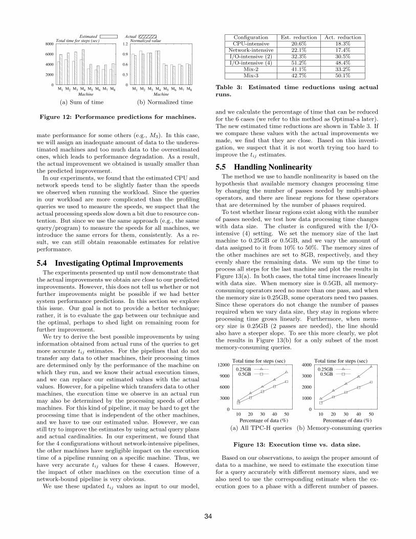
ing data processing times (the tijs). Thus, we want to seewhether our estimated times truly indicate the performancedifferences. For each machine in the cluster, we sum upits estimated and actual execution times for all steps. InFigure 12(a), we plot the results for the CPU-intensive con-figuration. In this case, the estimated workload executiontime is 5346 seconds, which is shorter than the actual execu-tion time of 7371 seconds. From the graph, we can see thatthe estimated times for all machines are consistently shorterthan the corresponding actual execution times. If we pickthe machine with the longest actual processing time (M4 inthe graph) and use the actual (estimated) time for it to nor-malize the actual (estimated) times for other machines, weget the normalized performance for all machines as shownin Figure 12(b). Ideally, we hope that for each machine itsnormalized estimated value is the same as the actual value.Although our estimates are not perfect, the errors we makewhen predicting relative performance differences are muchsmaller than when predicting absolute performance.

From Figure 12(b), we can also see that we underestimateperformance for some machines (e.g., M2) while overesti-

33

Estimated Actual

0

2000

4000

6000

8000

M1M

2M

3M

4M

5M

6M

7M

8

Machine

Total time for steps (sec)

0

0.3

0.6

0.9

1.2

M1

M2

M3

M4

M5

M6

M7

M8

Machine

Normalized value

(a) Sum of time (b) Normalized time

Figure 12: Performance predictions for machines.

mate performance for some others (e.g., M3). In this case,we will assign an inadequate amount of data to the underes-timated machines and too much data to the overestimatedones, which leads to performance degradation. As a result,the actual improvement we obtained is usually smaller thanthe predicted improvement.

In our experiments, we found that the estimated CPU andnetwork speeds tend to be slightly faster than the speedswe observed when running the workload. Since the queriesin our workload are more complicated than the profilingqueries we used to measure the speeds, we suspect that theactual processing speeds slow down a bit due to resource con-tention. But since we use the same approach (e.g., the samequery/program) to measure the speeds for all machines, weintroduce the same errors for them, consistently. As a re-sult, we can still obtain reasonable estimates for relativeperformance.

5.4 Investigating Optimal ImprovementsThe experiments presented up until now demonstrate that

the actual improvements we obtain are close to our predictedimprovements. However, this does not tell us whether or notfurther improvements might be possible if we had bettersystem performance predictions. In this section we explorethis issue. Our goal is not to provide a better technique;rather, it is to evaluate the gap between our technique andthe optimal, perhaps to shed light on remaining room forfurther improvement.

We try to derive the best possible improvements by usinginformation obtained from actual runs of the queries to getmore accurate tij estimates. For the pipelines that do nottransfer any data to other machines, their processing timesare determined only by the performance of the machine onwhich they run, and we know their actual execution times,and we can replace our estimated values with the actualvalues. However, for a pipeline which transfers data to othermachines, the execution time we observe in an actual runmay also be determined by the processing speeds of othermachines. For this kind of pipeline, it may be hard to get theprocessing time that is independent of the other machines,and we have to use our estimated value. However, we canstill try to improve the estimates by using actual query plansand actual cardinalities. In our experiment, we found thatfor the 4 configurations without network-intensive pipelines,the other machines have negligible impact on the executiontime of a pipeline running on a specific machine. Thus, wehave very accurate tij values for these 4 cases. However,the impact of other machines on the execution time of anetwork-bound pipeline is very obvious.

We use these updated tij values as input to our model,

Configuration Est. reduction Act. reductionCPU-intensive 20.6% 18.3%

Network-intensive 22.1% 17.4%I/O-intensive (2) 32.3% 30.5%I/O-intensive (4) 51.2% 48.4%

Mix-2 41.1% 33.2%Mix-3 42.7% 50.1%

Table 3: Estimated time reductions using actualruns.

and we calculate the percentage of time that can be reducedfor the 6 cases (we refer to this method as Optimal-a later).The new estimated time reductions are shown in Table 3. Ifwe compare these values with the actual improvements wemade, we find that they are close. Based on this investi-gation, we suspect that it is not worth trying too hard toimprove the tij estimates.

5.5 Handling NonlinearityThe method we use to handle nonlinearity is based on the

hypothesis that available memory changes processing timeby changing the number of passes needed by multi-phaseoperators, and there are linear regions for these operatorsthat are determined by the number of phases required.

To test whether linear regions exist along with the numberof passes needed, we test how data processing time changeswith data size. The cluster is configured with the I/O-intensive (4) setting. We set the memory size of the lastmachine to 0.25GB or 0.5GB, and we vary the amount ofdata assigned to it from 10% to 50%. The memory sizes ofthe other machines are set to 8GB, respectively, and theyevenly share the remaining data. We sum up the time toprocess all steps for the last machine and plot the results inFigure 13(a). In both cases, the total time increases linearlywith data size. When memory size is 0.5GB, all memory-consuming operators need no more than one pass, and whenthe memory size is 0.25GB, some operators need two passes.Since these operators do not change the number of passesrequired when we vary data size, they stay in regions whereprocessing time grows linearly. Furthermore, when mem-ory size is 0.25GB (2 passes are needed), the line shouldalso have a steeper slope. To see this more clearly, we plotthe results in Figure 13(b) for a only subset of the mostmemory-consuming queries.

12000

9000

6000

3000

05040302010

Percentage of data (%)

Total time for steps (sec)

0.25GB0.5GB

4000

3000

2000

1000

05040302010

Percentage of data (%)

Total time for steps (sec)

0.25GB0.5GB

(a) All TPC-H queries (b) Memory-consuming queries

Figure 13: Execution time vs. data size.

Based on our observations, to assign the proper amount ofdata to a machine, we need to estimate the execution timefor a query accurately with different memory sizes, and wealso need to use the corresponding estimate when the ex-ecution goes to a phase with a different number of passes.

34

For the system that we worked with, our technique is effec-tive when no more than one pass is needed. Take the I/O-intensive configuration as an example. We set the DBMSmemory size to 0.5GB (where no operator needs more thanone pass) for the last machine and 8GB for other machinesto repeat the experiment. The predicted and actual timereductions for our approach are 53.5% and 46.7%, respec-tively. The time estimates for the last machine correctlyrepresent its performance differences compared to other ma-chines, and thus less data is assigned to it compared to itsoriginal configuration with 8GB memory.

Strategy Bricolage-d Bricolage-g Optimal-aEst. reduction 53.1% 52.5% 46.7%Act. reduction 35.2% 44.1% 44.9%

Table 4: Percentage of time reductions when mem-ory size is 0.25GB for the last machine.

However, when memory is really scarce and more thanone pass is required, the I/O cost estimates provided by oursystem are no longer accurate. Our predicted times are usu-ally smaller than the actual processing times. In the firstcolumn of Table 4, we show the estimated and actual re-ductions in time for our default approach without guardingpoints (we refer to it as Bricolage-d in the table), when theDBMS memory size is set to 0.25GB for the last machine.This is a really adversarial situation, since the last machinehas the most powerful disks to accomplish more I/O workwhile at the same time, it does not have enough memoryto accommodate the data. The actual performance we ob-tained is much worse than our prediction, since we assigntoo much data to the last machine.

We have proposed two strategies in Section 4.4 for han-dling this: issuing a warning or using guarding points. Inthe above case, after we use Bricolage-d to provide an alloca-tion recommendation, we estimate the input size |S| for eachmemory-consuming operator as if data were partitioned inthe suggested way. We found that some operators need twopasses based on the estimated input table sizes and availablememory. Thus, we can issue a warning saying that we arenot sure about our estimate this time. Another approachdenoted as Bricolage-g is to use guarding points. For ma-chine Mi, we calculated a pisafe value, to ensure that as longas the data allocated to Mi is no more than pisafe , no op-erator needs more than one pass. As we can see from thetable, by using guarding points, our estimate is now moreaccurate. We also investigate the optimal improvement forthis case by using information derived from actual runs asinput parameters to the model. The results are shown inthe last column of Table 4. Although the actual reductionsfor Bricolage-g and Optimal-a are similar here, in general,an approach that uses true performance for machines canbetter exploit their capabilities. As a result, we leave ac-curate time estimation for memory-consuming operators asour future work.

5.6 Overhead of Our SolutionOur approach needs to estimate the processing speeds for

machines, estimate plans and their execution times, andsolve the linear model. Here, we describe the overheadsinvolved. In our experiments, we used 2 minutes each totest the I/O and the CPU speeds for a machine. This canbe done on all machines concurrently. We used 30 secondsto test the network speed for a machine, but another fast

machine is required for sending/receiving the data. In theworst case, where we use just one fast machine to do the test,we need 0.5n minutes to test all n machines. We think thisoverhead is sufficiently small. For example, we need only 50minutes to test the network speeds for 100 machines. Forthe complex analytical TPC-H workload, the average timeto generate plans and estimate processing times for a queryis 2.3 seconds. Thus the expected total time to estimate theperformance parameters for a workload is 2.3|W |, where |W |is the number of queries in the workload. After we get allthe estimates, the linear program can be solved efficiently.For example, for a cluster with 100 machines of 10 differentkinds, and a workload with 100 queries, the linear programsolver returns the solution in less than 3 seconds.

6. RELATED WORKOur work is related to query execution time estimation,

which can be loosely classified into two categories. The firstcategory includes work on progress estimation for runningqueries [5, 15, 16, 18, 19, 22]. The key idea for this work isto collect runtime statistics from the actual execution of aquery to dynamically predict the remaining work/time forthe query. In general, no prediction can be made before thequery starts. The debug run-based progress estimator forMapReduce jobs proposed in [24] is an exception. However,it cannot provide accurate estimates for queries running ondatabase systems [17]. On the other hand, the second cate-gory of work focuses on query running time prediction beforea query starts [4, 11, 13, 31, 32]. In [32] the authors proposeda technique to calibrate the cost units in the optimizer costmodel to match the true performance of the hardware andsoftware on which the query will be run, in order to estimatequery execution time. This paper gave details about how tocalibrate the five parameters used by PostgreSQL. However,different database optimizers may use different cost formu-las and parameters. Additional work is required before wecan apply the technique to other database systems. Usageof machine-learning based techniques for the estimation ofquery runtime has been explored in [4, 11, 13]. One keylimitation of these approaches is that they do not work wellfor new “ad-hoc” queries, since they usually use supervisedmachine learning techniques.

Another related research direction is automated partition-ing design for parallel databases. The goal of a partitioningadvisor is to automatically determine the optimal way ofpartitioning the data, so that the overall workload cost isminimized. The work in [14] investigates different multi-attribute partitioning strategies, and it tries to place tuplesthat satisfy the same selection predicates on fewer machines.The work in [7, 21] studies three data placement issues:choosing the number of machines over which to partitionbase data, selecting the set of machines on which to placeeach relation, and deciding whether to place the data ondisk or cache it permanently in memory. In [25, 27], themost suitable partitioning key for each table is automati-cally selected in order to minimize estimated costs, such asdata movement costs. While these approaches can substan-tially improve system performance, they focus on base tablepartitioning and treat all machines in the cluster as identi-cal. In our work, we aim at improving query performancein heterogeneous environments. Instead of always applyinga uniform partitioning function to these keys, we vary theamount of data that will be assigned to each machine for the

35

purpose of better resource utilization and faster query exe-cution. The work in [8, 26] attempts to improve scalabilityof distributed databases by minimizing the number of dis-tributed transactions for OLTP workloads. Our work tar-gets resource-intensive analytical workloads where queriesare typically distributed.

Our work is also related to skew handling in parallel databasesystems [10, 33, 34]. Skew handling is in a sense the dualproblem of the one that we deal with in the paper. It as-sumes that the hardware is homogeneous, but data skew canlead to load imbalances in the cluster. It then tries to levelthe imbalances that arise.

Finally, our paper is related to various approaches pro-posed for improving system performance in heterogeneousenvironments [3, 35]. A suite of optimizations are proposedin [3] to improve MapReduce performance on heterogeneousclusters. Zaharia et al. [35] develop a scheduling algorithmto dispatch straggling tasks to reduce execution times ofMapReduce jobs. Since a MapReduce system does not useknowledge of data distribution and location, our techniquecannot be used to pre-partition the data in HDFS. However,we can apply our technique to partition intermediate datain MapReduce systems with streaming pipelines.

7. CONCLUSIONWe studied the problem of improving database perfor-

mance in heterogeneous environments. We developed a tech-nique to quantify performance differences among machineswith heterogeneous resources and to assign proper amountsof data to them. Extensive experiments confirm that ourtechnique can provide good and reliable partition recom-mendations for given workloads with minimal overhead.

This paper lays down a foundation for several directionstowards future studies to improve database performance run-ning in the cloud. Previous research has revealed that thesupposedly identical instances provided by a public cloudoften exhibit measurable performance differences. One in-teresting problem is to select the set of most cost-efficient in-stances to minimize the execution time of a workload. Whilethe focus of this work has been on static data partitioningstrategies, the natural follow-up will be to study how to dy-namically repartition the data at runtime, when our initialprediction was not accurate or system conditions change.

AcknowledgmentThis research was supported by a grant from Microsoft JimGray Systems Lab, Madison, WI. We would like to thankeveryone in the lab for valuable suggestions on this project.

8. REFERENCES[1] SQL Server 2012 Parallel Data Warehouse.

http://www.microsoft.com/en-ca/server-cloud/products/analytics-platform-system/.

[2] S. Agrawal, V. Narasayya, and B. Yang. Integrating verticaland horizontal partitioning into automated physical databasedesign. SIGMOD, 2004.

[3] F. Ahmad, S. T. Chakradhar, A. Raghunathan, and T. N.Vijaykumar. Tarazu: Optimizing mapreduce on heterogeneousclusters. ASPLOS, 2012.

[4] M. Akdere, U. Cetintemel, M. Riondato, E. Upfal, and S. B.Zdonik. Learning-based query performance modeling andprediction. ICDE, 2012.

[5] S. Chaudhuri, R. Kaushik, and R. Ramamurthy. When can wetrust progress estimators for SQL queries? In SIGMOD, 2005.

[6] S. Chaudhuri, V. Narasayya, and R. Ramamurthy. Estimatingprogress of execution for SQL queries. In SIGMOD, 2004.

[7] G. Copeland, W. Alexander, E. Boughter, and T. Keller. Dataplacement in Bubba. SIGMOD Record, 1988.

[8] C. Curino, E. Jones, Y. Zhang, and S. Madden. Schism: aworkload-driven approach to database replication andpartitioning. PVLDB, 2010.

[9] G. B. Dantzig and M. N. Thapa. Linear Programming 1:Introduction. Springer-Verlag, 1997.

[10] D. J. DeWitt, J. F. Naughton, D. A. Schneider, and S. Seshadri.Practical skew handling in parallel joins. VLDB, 1992.

[11] J. Duggan, U. Cetintemel, O. Papaemmanouil, and E. Upfal.Performance prediction for concurrent database workloads.SIGMOD, 2011.

[12] B. Farley, A. Juels, V. Varadarajan, T. Ristenpart, K. D.Bowers, and M. M. Swift. More for your money: exploitingperformance heterogeneity in public clouds. SoCC, 2012.

[13] A. Ganapathi, H. Kuno, U. Dayal, J. L. Wiener, A. Fox,M. Jordan, and D. Patterson. Predicting multiple metrics forqueries: Better decisions enabled by machine learning. ICDE,2009.

[14] S. Ghandeharizadeh, D. J. DeWitt, and W. Qureshi. Aperformance analysis of alternative multi-attribute declusteringstrategies. SIGMOD, 1992.

[15] A. C. Konig, B. Ding, S. Chaudhuri, and V. Narasayya. Astatistical approach towards robust progress estimation.PVLDB, 2012.

[16] J. Li, R. V. Nehme, and J. F. Naughton. GSLPI: A cost-basedquery progress indicator. In ICDE, 2012.

[17] J. Li, R. V. Nehme, and J. F. Naughton. Toward progressindicators on steroids for big data systems. In CIDR, 2013.

[18] G. Luo, J. F. Naughton, C. J. Ellmann, and M. W. Watzke.Toward a progress indicator for database queries. In SIGMOD,2004.

[19] G. Luo, J. F. Naughton, C. J. Ellmann, and M. W. Watzke.Increasing the accuracy and coverage of SQL progressindicators. In ICDE, 2005.

[20] D. Mangot. EC2 variability: The numbers revealed.http://tech.mangot.com/roller/dave/entry/ec2 variabilitythe numbers revealed, 2009.

[21] M. Mehta and D. J. DeWitt. Data placement in shared-nothingparallel database systems. The VLDB Journal, 1997.

[22] C. Mishra and N. Koudas. A lightweight online framework forquery progress indicators. ICDE, 2007.

[23] K. Morton, M. Balazinska, and D. Grossman. Paratimer: aprogress indicator for MapReduce DAGs. In SIGMOD, 2010.

[24] K. Morton, A. Friesen, M. Balazinska, and D. Grossman.Estimating the progress of MapReduce pipelines. In ICDE,2010.

[25] R. Nehme and N. Bruno. Automated partitioning design inparallel database systems. SIGMOD, 2011.

[26] A. Pavlo, C. Curino, and S. Zdonik. Skew-aware automaticdatabase partitioning in shared-nothing, parallel OLTPsystems. SIGMOD, 2012.

[27] J. Rao, C. Zhang, N. Megiddo, and G. Lohman. Automatingphysical database design in a parallel database. SIGMOD, 2002.

[28] C. Reiss, A. Tumanov, G. R. Ganger, R. H. Katz, and M. A.Kozuch. Heterogeneity and dynamicity of clouds at scale:Google trace analysis. SoCC, 2012.

[29] J. Schad, J. Dittrich, and J.-A. Quiane-Ruiz. Runtimemeasurements in the cloud: observing, analyzing, and reducingvariance. In PVLDB, 2010.

[30] G. Wang and T. S. E. Ng. The impact of virtualization onnetwork performance of amazon EC2 data center. INFOCOM,2010.

[31] W. Wu, Y. Chi, H. Hacıgumus, and J. F. Naughton. Towardspredicting query execution time for concurrent and dynamicdatabase workloads. PVLDB, 2013.

[32] W. Wu, Y. Chi, S. Zhu, J. Tatemura, H. Hacigumus, and J. F.Naughton. Predicting query execution time: Are optimizer costmodels really unusable? In ICDE, 2013.

[33] Y. Xu and P. Kostamaa. Efficient outer join data skewhandling in parallel DBMS. PVLDB, 2009.

[34] Y. Xu, P. Kostamaa, X. Zhou, and L. Chen. Handling dataskew in parallel joins in shared-nothing systems. SIGMOD,2008.

[35] M. Zaharia, A. Konwinski, A. D. Joseph, R. Katz, andI. Stoica. Improving mapreduce performance in heterogeneousenvironments. OSDI, 2008.

36