Proceedings World Geothermal Congress 2010 Bali, Indonesia, 25-29 April 2010

1

Resistivity Structures of Lahendong and Kamojang Geothermal Systems Revealed from 3-D Magnetotelluric Inversions, A Comparative Study

Imam B. Raharjo1, Virginia Maris, Phil E. Wannamaker, David S. Chapman

Dept. of G&G, University of Utah, Frederick A. Sutton Bldg, 115 S. 1460 E Rm 283, SLC, Utah 84112, USA 1Pertamina Geothermal Energy, Menara Cakrawala 15th fl, Jl. MH Thamrin 9, Jakarta 10340, Indonesia

imam.raharjo@utah.edu, iraharjo@pgeindonesia.com

Keywords: Lahendong, Kamojang, magnetotellurics, MT, geothermal

ABSTRACT

Three-dimensional magnetotelluric (MT) inversions of Lahendong and Kamojang datasets have been performed to obtain their resistivity structures. Gauss-Newton finite diference method of Sasaki was used, with several modifications including changing the parameter step solution to modified Cholesky and invoking a different system of parameter smoothing weights. The 2005 and 2008 MT datasets were binned to sets of frequencies for efficient inversions and provided a depth range of sensitivity from ~100 m to ~5 km, where the final misfits were three and two respectively.

Lahendong field has a liquid dominated reservoir in the north part and a two-phase region in the south part. The current electricity production is 40MW. The inversion reveals a subsurface dome with the resistivity of 20-60 ohm.m covered by a conductor, e.g. <10 ohm.m, that depicts a propylytic reservoir encapsulated by geothermal clay caps. The peak of the dome is situated under Linau acidic lake. The conductor rapidly thickens and deepens to the north and west, and gradually thickens to the south indicating a deeper prospect. The biggest well LHD-23, >35MW, penetrates the center block of the dome, where the propylitic region at 1.5 km deep is about 3x4 km2.

Kamojang on the other hand, is a vapor system hosted in a caldera surrounded by volcanic ranges. The fumaroles are situated in the north-east corner of the caldera at a higher elevation. The inversion reveals a spectacular finding. At a shallow depth, a conductor from the fumarolic area extends down to the caldera and merges with the conductive formations. The conductor becomes pervasive with depth down to about one km where the propylitic zone starts taking places. Within the production depth, e.g. 1.5 km, a subsurface u-shape proplytic ridge facing west is observed. The ridge represents the vapor zone that feeds the 200MW power plants. The shape of the ridge opens and vanishes to the west where the region becomes more conductive and associates with two-phase characteristics. An intriguing vertical resistive column, e.g. ~ 100 ohm.m feeding the Kamojang fumarolic area is also observed. The inversion suggests that the Kamojang caldera structure dictates the subsurface u-shape propylitic ridge in a steam dominated region.

1. INTRODUCTION

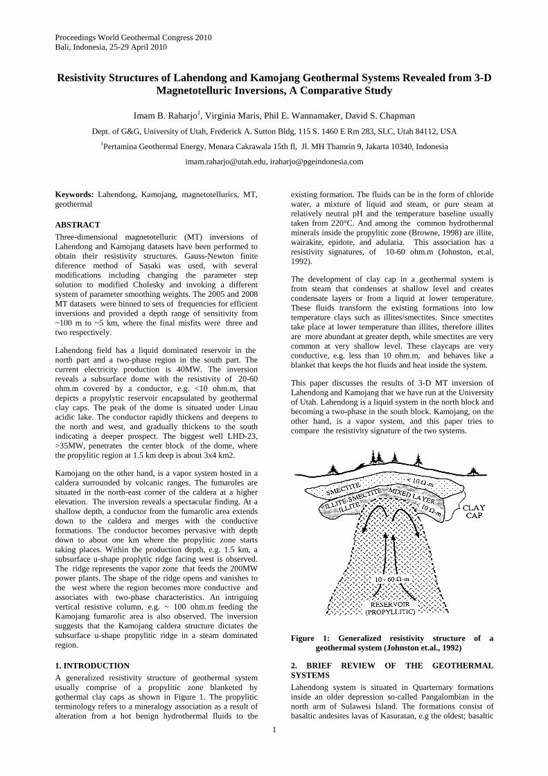
A generalized resistivity structure of geothermal system usually comprise of a propylitic zone blanketed by gothermal clay caps as shown in Figure 1. The propylitic terminology refers to a mineralogy association as a result of alteration from a hot benign hydrothermal fluids to the

existing formation. The fluids can be in the form of chloride water, a mixture of liquid and steam, or pure steam at relatively neutral pH and the temperature baseline usually taken from 220°C. And among the common hydrothermal minerals inside the propylitic zone (Browne, 1998) are illite, wairakite, epidote, and adularia. This association has a resistivity signatures, of 10-60 ohm.m (Johnston, et.al, 1992).

The development of clay cap in a geothermal system is from steam that condenses at shallow level and creates condensate layers or from a liquid at lower temperature. These fluids transform the existing formations into low temperature clays such as illites/smectites. Since smectites take place at lower temperature than illites, therefore illites are more abundant at greater depth, while smectites are very common at very shallow level. These claycaps are very conductive, e.g. less than 10 ohm.m, and behaves like a blanket that keeps the hot fluids and heat inside the system.

This paper discusses the results of 3-D MT inversion of Lahendong and Kamojang that we have run at the University of Utah. Lahendong is a liquid system in the north block and becoming a two-phase in the south block. Kamojang, on the other hand, is a vapor system, and this paper tries to compare the resistivity signature of the two systems.

Figure 1: Generalized resistivity structure of a geothermal system (Johnston et.al., 1992)

2. BRIEF REVIEW OF THE GEOTHERMAL SYSTEMS

Lahendong system is situated in Quarternary formations inside an older depression so-called Pangalombian in the north arm of Sulawesi Island. The formations consist of basaltic andesites lavas of Kasuratan, e.g the oldest; basaltic

Raharjo et al.

2

andesite lava dan pyroclatic deposits of Tampusu; andesitic basalt lava with obsidian and tuff of G.Lengkoan, and the youngest hydrothermal breccias of Linau (Siahaan et.al., 2005). Figure 2 shows the situation map of the Lahendong.

701 702 703 704 705 706 707137

138

139

140

141

142

143

775

775

775

800

825

825

825

825

850

850

850

850

875

875

875

900

900

00

900

925

925

925

925

950

950

950975

975

975

1000

1000

1000

1025

1025

1025

1050

1050

1075

1075

1100

1100

easting, km. datum WGS-84 51 North

nort

hing

, km

40MW p.plants

Lake Linau

6

11

15 8 9

1017

1814

7 5

1

16

19

12 4

2

23

Figure 2: Map showing the Lahendong area and vicinity, numbers show the wells, while dots are MT sites

Thermal expression at the surface is shown by hotsprings, fumaroles, steaming ground, mudpool, and a huge hydrothermal vent namely Lake Linau. In some places the fumaroles are superheated. From the downhole measuremet we observe the temperature of the field varies from about 280 and exceeding 320 °C. The geological structures contribute important role in the permeability of the reservoir and the surface manifestations. The system is liquid dominated at lower temperature in the northern part, and gradually changes into a hotter two phase system in the south. The field currently produces 40MW, with another development on the way.

802 803 804 805 806 807 808 809 810 811 812 8139204

9205

9206

9207

9208

9209

9210

9211

9212

9213

9214

1050

1075

1075

1100

1100

1100

1100

1125

1125

1125

1125

1150

1150

1150

1175

1175

1200

1200

1200

1225

1225

1225

1250

1250

1275

1275

1275

1275

1275

1300

1300

1300

1300

1325

1325

1325

1350

1350

1350

1375

1375

1400

1400

1400

1425

1425

1425

1450

1450

1475

1475

1500

1500

1500

1500

1525

1525

1525

1525

1525

1550

1550

1550

1550

1550 1550

1550

1550

1575

1575

1575

1 575

1575

1575

1575

1600

1600

1600

1600

1600

1600

1600

16251625

1625

1625

1625

1650

1650

1650

1650

1650

1650

1675

1675

1675

1675

1675

1675

1675

1700

1700

1700

1700

1700

1700

1725

1725

1725

1725

1725

1725

1750

1750

1750

1750

1750

1750

1775

1775

1775

1775

1775

1775

1800

1800

1800

1800

1800

1800

1825

1825

1825

1825

1825

1850

185 0

18501850

1875

1875

1875

1900

1900

1900

19251950

1975

2000

20252050

Easting, km

Nor

thin

g, k

m

o MT station/ well track

ℵ fumarolic area⊗ p.plants 140MW⊕ p.plant 60MW

contours in meter

WGS84 48South

Calderaoutline

Figure 3: Map showing the Kamojang area and vicinity, lines show the wells trajectory, while dots are the MT sites. Kendang fault is indicated by the straight contour break aligned NE, and the flat area at the center indicates the caldera

Kamojang is a geothermal system located in West Java and hosted inside a series of Quarternary volcanic formations.

Many investigators divided the series into more detailed formations, and for the purpose of this paper we considered the lithology as mostly andesite lavas and pyroclastic rocks. The prominent structure in Kamojang is a circular depression at the center and a north east trending Kendang Fault as shown in Figure 3. The surface expression from the upwelling regime is situated north east of the caldera, where fumaroles associated with altered ground, mudpool, and hotsprings are found. The temperature of the production portion of Kamojang reservoir varies from 220 to 245°C. The field currently produces 200 MW of electricity from four sets of turbine-generators.

3. MAGNETOTELLURIC & INVERSION METHOD

Magnetotelluric (MT) signals are natural electromagnetic wave fields induced by magnetospheric or ionospheric currents. The signals are used to image the resistivity structure of the earth (Vozoff, 1991; Jiracek et al., 1995). Since the source far from the survey area, MT waves can be treated as planar (Zhdanov and Keller, 1998). The waves propagate in a conducting earth diffusively (Vozoff, 1991). The second theorem of Maxwell's equations states that

t

BE

∂∂−=×∇ (1)

where E and B are electric and magnetic fields respectively. If the electrical properties of earth material are constant and independent of frequency, and the method employs low frequency signals where there are no dielectric displacement currents, equation (1) takes the form

)ˆˆ(

0

00

ˆˆˆ

0 ydHxdHi

EEz

zdydxd

yx

yx

+=

⎥⎥⎥⎥

⎦

⎤

⎢⎢⎢⎢

⎣

⎡

∂∂ ωµ

(2)

where ω is angular frequency, the induced magnetic field due to the existence of material is denoted as H, magnetic permeability is denoted as µo, and B=µoH. Since the plane wave propagates perpendicular to the earth surface, the vertical electric field (Ez) and its derivatives in x and y directions are zero. Expanding this equation and applying the Helmholtz solution (Zhdanov and Keller, 1998), we end up with two sets of apparent resistivities as function of frequency derived from the impedances:

H

E12

y

x

oxy ωµ

ρ = , and H

E12

x

y

oyx ωµ

ρ −= . (3)

In MT field campaign, we measure the orthogonal electric and magnetic fields as shown in Figure 4. We have used the x-axis being positive north, and the y-axis being positive east, while the z-axis is positive down.

Figure 4: Schematic diagram of MT field setup, where two pairs of orthogonal electric and magnetic fields are recorded

Raharjo, et al.

3

A robust remote reference was deployed to improve the data quality. This implementation yielded the overall quality of the data being excellent as shown in the Figure 5. As we have shown here, the figure exhibits excellent apparent resistivity and phase curves downto about 3000 seconds.

10-3

10-2

10-1

100

101

102

103

104

100

101

102

103

Period, seconds

App

aent

res

istiv

ity,

ohm

.m • xy, + yx

10-3

10-2

10-1

100

101

102

103

104

-150

-100

-50

0

50

100

150

Period, seconds

Pha

se,

degr

ee

Figure 5: An example of an excellent MT data taken during the campaign

3.1 Lahendong Inversion

Thirty five MT tensors were used for the 3-D inversion with a spacing varies from 1-2.5 km. The static shift of the tensors due to local topography have been corrected using TDEM. The inversion program was finite difference, with Gauss-Newton algorithm (Sasaki, 2004) obtained through a cooperative agreement. The size of the grid is 115×91×40 nodes in x-y-z direction. The inversion domain is 31×25×25. The lateral size of the cells inside the interested area is 150 meter, while the vertical size grows with depth, started from 40’s and became 200’s meters within the target depth.

During the inversion, the algorithm is designed to modify/ update the parameter step solutions, with Cholesky decomposition. In addition, regularization to the weighting parameter for smoothing is also carried out. The regularization is based on the adherence to apriori model, damping curvature, and vertical weighting as a function of depth. Cells located at shallow depth have smooth inversion parameter, and then under relaxation toward greater depth. The approach is in accordance with the relative influence from the individual parameter to the response. To achieve efficient inversion, the data are binned into 12 frequencies from 32 until 0.056 Hz on the basis of Gauss Method. The simplification is considered to be adequate to represent the frequency variation of the data and provides sensitivity range of depth from about ~100 m up to 5 km. The cell size ratio is also affects to the output response stability.

In general, the quality of the data is excellent down to 0.1 Hz, and some sites start to exhibits errors around this frequency. However, the error does not affect for the investigation of the resistivity structure within geothermal exploration depth range. The lower limit in the inversion is about ~2 % for the apparent resistivity and about ~1-1,5 degree for the phase, both for rhoxy and rhoyx modes. The convergence in general is obtained within six iterations. The convergence starts from a misfit of about 15 and ends at about three. For an ideal Gaussian dataset, in general there is no difficulties to reach an RMS of about one. For the

Lahendong dataset, we have a slightly larger error than the nominal error that are tabulated in the original EDI files. This is a typical real case even for a high quality data.

Prior to the inversion, the static distortion in the MT tensor have been corrected using TDEM dataset. However, partially, a slightly deviation from TDEM correction is found. In this research, the inversion was applied to both with static shift implementation and without static shift implementation. Similar results were obtained. And this paper displays the model with static shift implementation.

3.2 Kamojang Inversion

For the Kamojang case, we use thirty nine MT tensors with a spacing shown in the Figure 3. The size of the grid is 63×69×38 nodes in x-y-z direction, while the inversion domain is 34×37×24. To data are binned into 11 frequencies from 62 until 0.18 Hz on the basis of Gauss Method. The lateral size of the cells inside the interested area is 150 meter, while the vertical size grows with depth, started from 40’s and 200’s meters within the target depth.

Error floors equivalent to 2 log10 % apparent resistivity and 1-1/3 deg impedance phase were imposed for both modes of data. Convergence was achieved typically in five iterations with a starting normalized RMS misfit near 10 and ending near two. With an ideal Gaussian data set having no other complications, achieving an RMS near one is sought. In this data set, scatter in the data points was greater than the nominal error bars supplied with the original EDI listings, and somewhat greater even than the error floors stated above. This is a typical experience with field data, even that of the highest quality. This fit overall is quite good, with only limited outliers and even there the features of the data are qualitatively fit.

4. RESISTIVITY STRUCTURE OF LAHENDONG

The 3-D MT inversion result of Lahendong shows the existence of an updome resistivity structure, with the upwelling region situated under the Lake Linau. Three selected slices at different depth are shown to exhibit the dome, and each of them is shown in Figure 6, Figure 7, and Figure 8 respectively. The slices are also shown in 3-D view running from shallower to greater depth so that we can visualize the dome. Lake Linau is also shown by the gray area on the topographic mesh, and the average elevation is taken as 700 meters above sea level (masl.). The top surface of the 3-D block model is referred to this level, and the grid is also oriented to the north-east axis. The resistivity value is color coded as shown by the colorbar in each figure. We use hot color for conductive and the cool color for very resistive. The color gradation from yellow, light green to cyan represents a resistivity ranging from 10, 60, to 100 ohm.m. And this color spectrum is our main interest.

At this shallow level we observe a conductor layer concentrated in the vicinity of Lake Linau. The observation is shown by the slice in Figure 6. The size of the slice is about 5×5 km2, 125 meters thick, and situated at the elevation from 475 to 600 masl. The orientation of the conductor more or less is east-west in the south of Lake Linau and curling to the north west in the north of the lake. Beyond these blocks more resistive region is observe, as shown by the greenish to slightly blue color.

At a slightly deeper level we observe the conductor layer extents wider and enclose an interesting region. As shown by the second slice in Figure 7, the thickness of the slice is 160 m, and is situated at the elevation from 40 to 200 masl.

Raharjo et al.

4

The conductor circles a slightly resistive region, e.g. 20-60 ohm.m, shown by the yellow to cyan colored blocks. The interesting zone is situated right under the Lake, with an elongated shape trending ENE-WSW, and curling to the south at the southern end.

At a greater depth we observe the interesting region enclosed by the conductors extends even wider. As shown by the Figure 8, the extent is about 3×4 km2. At this level, the thickness of the slice shown is 200 m, while the position is situated from -700 to -500 masl, or abut 1.4 km from the average ground level of 700 masl. The shape of the enclosure more or less is circular under the lake, and extending to the south at a greater depth. The configuration of three slices is quite convincing to show the existence of a subsurface resistivity updome under Lake Linau. The dome also has a steeper side in the north and a gentler side in the south.

Figure 6: Three-dimesional view of resistivity structure of Lahendong at shallow depth. The slice is situated at 475 - 600 masl

Figure 7: Three-dimesional view of the resistivity structure of Lahendong shown by the horizontal slice located at 40 - 200 masl. Well track LHD23 is shown

Figure 8: Three-dimesional view of the resistivity structure of Lahendong at a depth of 1.5 km overlain by topographic mesh. Well track LHD23 is shown. Slice thickness is 200 m, situated at -0.7 to -0.5 masl

5. RESISTIVITY STRUCTURE OF KAMOJANG

Similar display technique is used for the Kamojang 3-D grid. The average elevation of 1500 masl is the reference for the very top surface of the 3-D grid. The grid originally is oriented to N48E following the major structural trend in the vicinity, and we have plotted the grid superimposed on the north-east axis as shown in the Figure 9, Figure 10, and Figure 11. The existing wells and the topography margins are also displayed to give a comprehensive three dimensional view of the field.

At a very shallow depth, we observe two spots of conductive area, as marked by A and B in the Figure 9. Not surprisingly, the conductor A is associated with surface thermal expression while the conductor B is the respond from the caldera-fill materials. At a shallow-intermediate depth, the conductors merge and become pervasive as shown in the Figure 10. The thickness of the slice in this figure is 125 m thick, and situated from 925 to 1050 masl. Another finding in the figure is a spot of slightly resistive region under the fumarolic area.

Figure 9: Three-dimesional view of resistivity structure of Kamojang at shallow depth. Two shallow conductive spots marked A and B are underlined in the text. The 60m thin slice is situated at 1400 - 1460 masl

Raharjo, et al.

5

Figure 10: Three-dimesional view of resistivity structure of Kamojang at an intermediate depth, e.g 925-1050 masl, 125 m thick. A pervasive conductor is observed

At a greater depth the conductors take place on the margin and enclosing a slightly resistive region (20-60 ohm.m) as shown by the slice in the Figure 11. The thickness of the slice is 200 meters, situated from 125 masl down to -75 masl. In the west, the south, and east regions, the conductors perfectly seal the interesting areas. While in the central area we observe a u-shape ridge facing to the west circled by the conductors. Another attractive observation is the spot under the thermal expression area. The spot has become more resistive compared to the other regions. In the north side of the slice the conductors are not fully sealing the interesting region, since two continuous elongated bodies extending out to the north and the north west are found. Thus, more MT sites further to the north are still needed so that we could draw the north boundary.

802804

806808

810812

814

9204

9206

9208

9210

9212

9214

0

1

2

northing, km

easting, km. datum WGS84 48South

elev

atio

n, k

m

1|

10|

100|

1000|

Ω .m

Figure 11: Three-dimesional view of the resistivity structure of Kamojang at a productive depth. The 200-m slice is situated from -0.075 to 125 masl. U-shape propylitic ridge is observed

DISCUSSION

The resistivity structure of Lahendong shows rather simple dome of a proplytic zone encapsulated by hydrothermal clay cap. The very shallow conductor in the vicinity of Lake Linau is associated with the shallow hydrothermal alteration that we have seen in the field. In this area we found altered ground, superheated fumaroles, and acidic mudpool. The existence of altered ground and acidic mudpool are from the

shallow acid zone as the result from H2S from the deep being oxidized to create sulphuric acid. The acid alters the host rocks and transforms them into clays, such as smectites and kaolins. Shallow slim holes drilled during the early stages of the exploration have confirmed the existence of this acid shallow zone.

LHD-23 is the biggest liquid well in Lahendong with the production capacity exceeding 35 MW,and it is shown in Figure 6, Figure 7, and Figure 8. This is a deviated well having the total depth of 2000 m and that penetrates the clay caps and the 20-60 ohm.m propylitic zone. From the drilling records, the argilic conductor having a composition of about 50-60 percent clays was found down to the depth of about ~1100 m. At this section the lithology was dominated by hydrothermally altered tuff breccias and andesite lava. The appearance of epidote, the key mineral to propylitic zone, was found at a depth of ~1240 m, followed by partially loss circulation fluid at a depth of ~1360 m. The total loss circulation started at a depth of ~1700 m until the final depth. The production test of LHD-23 shows the potency of >35 MW, and one of the biggest well in Pertamina own operation. From resistivity point of view, the well penetrates the upwelling region of the dome shape structure. From this study the wells that located in the south west corner of the prospect penetrate the edge of the interesting blocks, and a appropriate maneuvers are needed to have a better production.

The resistivity structure of Kamojang shows rather a more complicated configuration. At a shallow depth, a conductor from the fumarolic area extends down to the caldera and merges with the conductive formations creating a pervasive clay caps. Keep in mind, this widely extent conductor may represent a geothermal clay caps, weathered layer on a volcano flank, and caldera-fill deposits. The caps, or combination of them, create a perfect blanket for the Kamojang geothermal system. The clay caps are quite extensive down to about 500 meters and gradually decrease down to about a kilometer. Beyond this level we find the propylitic reservoir that has been proven by drilling. The Kamojang propylitic zone contains wairakite and epidote (Utami and Browne, 1999).

The propylitic zone in Kamojang as interpreted from the resistivity structure, has a u-shape ridge that faces west. This zone currently provides the steam for the 200 MW power generation, especially from the north and west arms. In the north east portion of the ridge we also observe a vertical resistive column pointing up to the fumarolic area. This spot is interpreted as the upflow zone of the system, and will be an interesting object for a further research . On the west part of the u-shape propylitic zone we observed a conductive spot. This portion has been drilled and it has a slightly different characteristics, e.g the reservoir contains liquid. The model suggests size of the propylitic zone is about 5×4 km2, excluding the questionable spots on the north and north west margins.

CONCLUSIONS

Three-dimensional magnetotelluric inversions of Lahendong and Kamojang geothermal systems have been performed. Lahendong model yields a simple propylitic dome having the resistivity of 20-60 ohm.m encapsulated by a conductive clay cap of less than 10 ohm.m. The peak of the dome is pointing to the acidic Lake Linau and situated about 500 m underground. At a depth of about 1.5 km the size of the dome is about 3×4 km2. Kamojang model on the other hand exhibits a widely spread clay cap situated down to about one km underground. The cap is slightly elevated in the

Raharjo et al.

6

vicinity of the fumarolic area. Underneath the widespread cap the propylitic zone is found having a u-shape ridge facing west, and possibly controlled by the caldera structure. The model implies the size of the propylitic zone of about 5×4 km2. In the north east portion of the propylitic zone a vertical resistive column feeding the fumarolic area is also found, and this feature is very intriguing as a subject for further research. Further work that we would like to perform is to constrain the model with other geologic information or possibly downhole logging data.

ACKNOWLEDGMENT

Dr. Yutaka Sasaki for providing the 3-D codes through Phil Wannamaker.

PT Pertamina Geothermal Energy BOD’s for providing the funding for the PhD of the first author at the University of Utah, Salt Lake City, USA.

REFERENCES

Browne, P.R.L. : Hydrothermal Alteration, 665.611 Class Notes, Geothermal Institute, The University of Auckland, (1998)

Jiracek, G.R., Haak, V., and Olsen, K.H.: Practical Magnetotellurics in a continental rift environment, in Continental Rifts: Evolution, Structure and Tectonics, pp 103-129 (1995)

Johnston, J.M., Pellerin, L. and Hohmann, G.W. : Evaluation of Electromagnetic Methods for

GeothermalReservoir Detection. Geothermal Resources Council Transactions, Vol 16. pp 241 – 245 (1992)

Sasaki, Y. : Three-dimensional Inversion of Static Shifted Magnetotelluric Data, EarthPlanets Space, 56, 239-248 (2004).

Siahaan, E.E., Soemarinda, S., Fauzi, A., Silitonga, T., Azimudin, T., and Raharjo, I.B., Tectonism and Volcanism Study in the Minahasa Compartment of the North Arm of Sulawesi Related to Lahendong Geothermal Field, Indonesia, Proc. World Geothermal Congress, Antalya (2005)

Utami, P. and Browne., P.R.L.: Subsurface Hydrothermal Alteration in the Kamojang Geothermal Field, West Java, Indonesia, Proc. 24th Workshop on Geothermal Reservoir Engineering, Stanford, California (1999)

Vozoff, K.,: The magnetotelluric method, in Electro-magnetic methods in applied geophysics, ed.by Nabighian, M. N., v. 2B. Soc. Explor. Geophys.,Tulsa, 641-711 (1991).

Wannamaker, P.E., Stodt., J.A., and Rijo, L.: A stable Finite Element Solution for Two Dimensional agnetotelluric modeling, Geophy, J. Roy., Astr. Soc. (1987)

Zhdanov, M.S., Keller., G.V.: 1994, The Geoelectrical Methods in Geophysical exploration, Elsevier (1994)

Zhdanov, M.S.: Geophysical Inverse Theory and Regularization Problem, Elsevier (2002)