Embed Size (px)
Citation preview
Residual Stress Measurement of AISI 304 Stainless Steel
Nuclear Canister Plates by X-ray Diffraction
A Major Qualifying Project report to be submitted to the faculty of
WORCESTER POLYTECHNIC INSTITUTE in partial
fulfillment of the requirements for the Degree of Bachelor of Science
Submitted By
Jessica Ma
Submitted on
April 23rd,2015
Approved by:
Professor Richard Sisson
2
Abstract
The nuclear fuel storage canisters are used to store spent fuel of the nuclear plants. However,
some of the storage sites are located near the sea coast which the environment has high chloride
concentration. Such environment along with the residual stress in the AISI 304 stainless steel
canister plates caused by welding make them susceptible to stress corrosion cracking. The goal of
this project is to study the residual stress in the plates by performing X-ray diffraction method.
The macro and micro hardness as well as microstructure of the plates were also measured and
examined.
3
Acknowledgement
I want to thank both of my advisors, Professor Richard Sisson from Worcester Polytechnic
Institute, and Professor Ronald Ballinger from Massachusetts Institute of Technology for their
advices and support. I really appreciate that I have an opportunity to work on this amazing project.
I would gratefully acknowledge the support of Dr. Boquan Li from Worcester
Polytechnic Institute and Mr. Peter Stahle from Massachusetts Institute of Technology on sample
preparation and instrument training. I also would like to thank graduate students from WPI, Yuan
Lu and Haixuan Yu, for their valuable time and generous support to help me to achieve the goals
of this project.
This work was supported by the H.H. Uhlig Corrosion Lab’s project of the Life
Prediction of Spent Fuel Storage Canister Material, which is funded by U.S. Department of
Energy under Award Number: DE-AC07-051D14517
4
Contents Abstract ......................................................................................................................................................... 2
Acknowledgement ........................................................................................................................................ 3
Table of Figures ............................................................................................................................................. 6
Introduction .................................................................................................................................................. 7
Background ................................................................................................................................................... 9
Residual Stress .......................................................................................................................................... 9
Residual Stress Induced by Welding ....................................................................................................... 11
AISI Stainless Steel 304 ........................................................................................................................... 11
Contour Method ..................................................................................................................................... 13
X-ray Diffraction ...................................................................................................................................... 16
Neutron Diffraction Method ................................................................................................................... 18
Hole Drilling Method ............................................................................................................................... 20
Methodology ............................................................................................................................................... 22
Young’s Modulus ..................................................................................................................................... 22
Macro and Micro Hardness ..................................................................................................................... 23
Microstructure ........................................................................................................................................ 24
Phase Identification by Using X-ray Diffraction ...................................................................................... 24
Sample Annealing & Strain-free Lattice Parameter Determination ....................................................... 25
Stress Measurement by X-ray Diffraction ............................................................................................... 26
Results and Discussion ................................................................................................................................ 32
Elastic Modulus ....................................................................................................................................... 32
Macro and Micro Hardness ..................................................................................................................... 32
Microstructure ........................................................................................................................................ 33
Phase Identification ................................................................................................................................ 34
Strain Free Lattice Parameter ................................................................................................................. 35
Stress Calculation .................................................................................................................................... 36
Normal Stress .......................................................................................................................................... 37
Stress Measurements ............................................................................................................................. 37
Set One ................................................................................................................................................ 37
Set Two................................................................................................................................................ 43
Discussion ............................................................................................................................................ 48
Conclusion ................................................................................................................................................... 51

5
Bibliography ................................................................................................................................................ 53
Appendices .................................................................................................................................................. 55
Appendix A Sample Data Calculation .................................................................................................... 55
Appendix B Sample Neutron Diffraction Data ........................................................................................ 57
6
Table of Figures Figure 1. Dry Cask Storage System [3] .......................................................................................................... 8
Figure 2. Superposition Principle for Contour Method; Stresses are Plotted on One Quarter of the
Original Body [9] ......................................................................................................................................... 14
Figure 3. Averaging Two Contours to Eliminate Anti-symmetric Errors [9] ................................................ 15
Figure 4. Bulge Error Effect [9] .................................................................................................................... 16
Figure 5. Diffraction within a crystal structure, d denotes for inter lattice spacing, ϴ denotes for Bragg
angle, λ denotes for wavelength. [10] ........................................................................................................ 17
Figure 6.Schematic of X-ray diffraction on (a) unstressed state and (b) stressed state under applied load.
[10] .............................................................................................................................................................. 17
Figure 7. . Schematic of neutron diffraction setup, the gage volume is the intersection between the
incident beam and the diffracted beam, the scattering vector Q bisects the intersection. [11] ............... 19
Figure 8. Schematic of Hole Drilling Method, A, B, C Denote the Strain Gage. .......................................... 21
Figure 9. Standardized Hole Drilling Strain Gage Rosettes [12] .................................................................. 21
Figure 10. Hole drilling machines (a) SINT MTS 3000 and (b) Micro-Measurement RS-200 [12] ............... 21
Figure 11. AISI 304 Stainless Steel Sample with Large Size ......................................................................... 23
Figure 12. AISI 304 Stainless Steel Sample with Small Size ......................................................................... 23
Figure 13. Electrochemical Etching ............................................................................................................. 24
Figure 14. AISI 304 Medium-size Sample with a Dimension of 10cm*5cm*2cm ....................................... 25
Figure 15. Medium-size Sample with Measurement Points ....................................................................... 27
Figure 16. Schematic of Stress Measurement in XRD [14] ......................................................................... 28
Figure 17. Actual Experimental Setup ......................................................................................................... 28
Figure 18.Strain Directions on Actual Sample............................................................................................. 29
Figure 19. Biaxial Stress State with Linear Behavior ................................................................................... 30
Figure 20. Triaxial Stress State- ψ Splitting Behavior .................................................................................. 30
Figure 21. Micro Hardness on Eight Small Samples .................................................................................... 33
Figure 22. Microstructure of AISI 304 Stainless Steel Sample .................................................................... 34
Figure 23. Phase Identification Diagram of AISI 304 Sample ...................................................................... 35
Figure 24. (a) Linear Behavior with Small Shear Stress; (b) ψ Splitting Behavior with Larger Shear Stress
(triangle indicates data measured at positive ψ and square indicates data measured at negative ψ) ..... 37
Figure 25. Normal Stress Distribution across the Sample........................................................................... 39
Figure 26. Transverse Stress Distribution across the Sample (orange line represents the triaxial state and
blue line represents the biaxial state) ........................................................................................................ 41
Figure 27. Longitudinal Stress Distribution across the Sample (orange line represents the triaxial state
and blue line represents the biaxial state) ................................................................................................. 43
Figure 28.Normal Stress Distribution across the Sample ........................................................................... 44
Figure 29.Transverse Stress Distribution across the Sample (orange line represents the triaxial state and
blue line represents the biaxial state) ........................................................................................................ 46
Figure 30. Longitudinal Stress Distribution across the Sample (orange line represents the triaxial state
and blue line represents the biaxial state) ................................................................................................. 48
Figure 31. Residual Stress Distribution across the Sample: 1-longtudinal stress; 2-Transverse Stress [18]
.................................................................................................................................................................... 49
Figure 32. Normal Residual Stress Distribution in Welded Samples [19] ................................................... 49
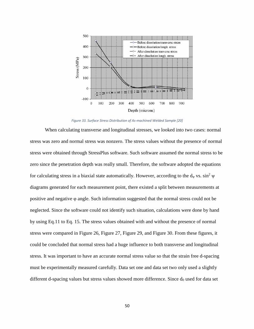
Figure 33. Surface Stress Distribution of As-machined Welded Sample [20] ............................................. 50
7
Introduction The spent nuclear fuel is expected to be stored on the fuel rods at the nuclear plants. In
service, these rods need to be changed periodically because they tend to lose efficiency over
time. When the rods are replaced, the spent fuel that already existed in the rods will be moved to
the pools of water at the reactor site where the fuel will be kept safely. The newly generated
spent fuel will fill up the new rods in the plants and such process occurs over and over again. In
early 1980s, the pools were found having a low capacity and the concept of dry storage cask
canisters appeared. [1] A typical storage cask canister has a metal cylinder which contains the
spent fuel and such canister is surrounded by a metal or concrete cask to prevent radiation. The
cask system is safe and environmentally friendly which it provides heat management, radiation,
and nuclear fission containment. Such system also resists earthquake, projectiles, tornadoes,
floods, temperature extremes and others natural or human related catastrophes. The spent fuel in
the canister only emits a little amount of heat and its heat emission and radioactivity decrease
over time. Therefore, the dry cask system provides the maximum safety for nuclear fuel storage.
[2]
8
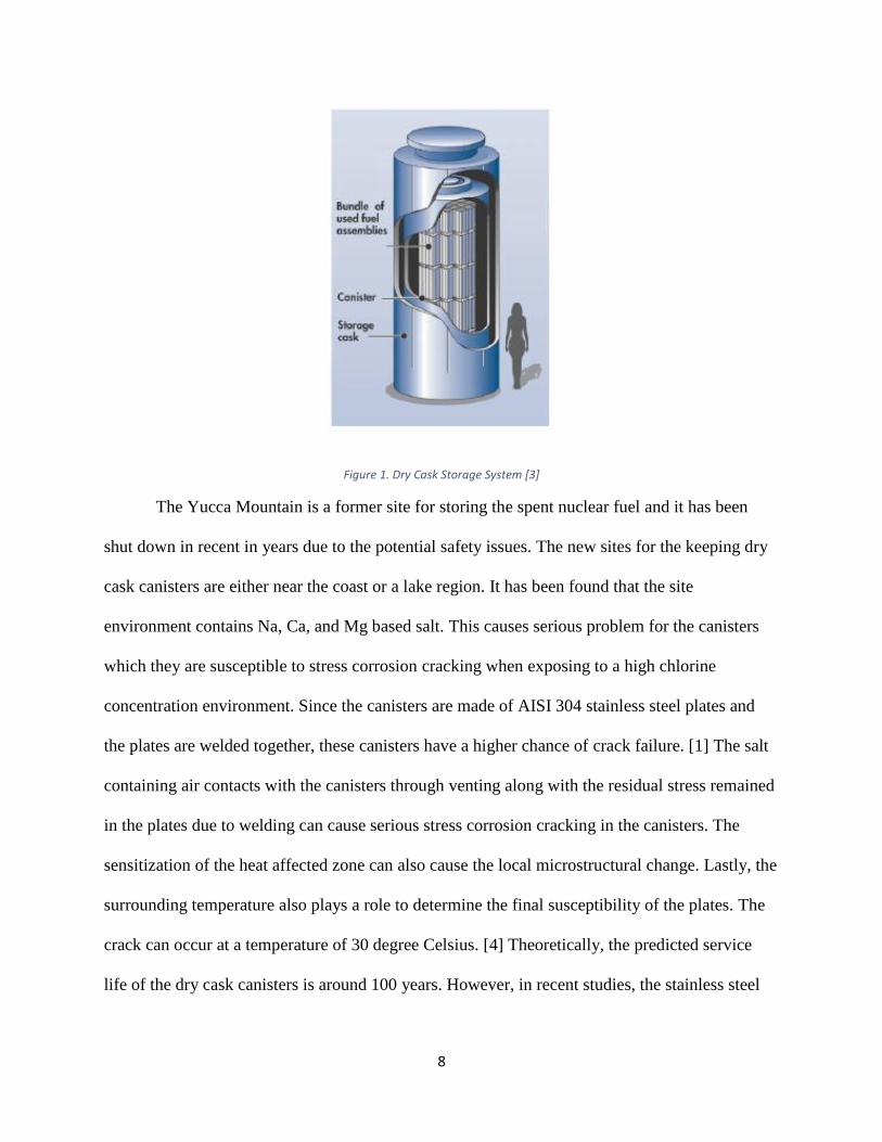
Figure 1. Dry Cask Storage System [3]
The Yucca Mountain is a former site for storing the spent nuclear fuel and it has been
shut down in recent in years due to the potential safety issues. The new sites for the keeping dry
cask canisters are either near the coast or a lake region. It has been found that the site
environment contains Na, Ca, and Mg based salt. This causes serious problem for the canisters
which they are susceptible to stress corrosion cracking when exposing to a high chlorine
concentration environment. Since the canisters are made of AISI 304 stainless steel plates and
the plates are welded together, these canisters have a higher chance of crack failure. [1] The salt
containing air contacts with the canisters through venting along with the residual stress remained
in the plates due to welding can cause serious stress corrosion cracking in the canisters. The
sensitization of the heat affected zone can also cause the local microstructural change. Lastly, the
surrounding temperature also plays a role to determine the final susceptibility of the plates. The
crack can occur at a temperature of 30 degree Celsius. [4] Theoretically, the predicted service
life of the dry cask canisters is around 100 years. However, in recent studies, the stainless steel
9
piping in the nuclear plants suffered from stress corrosion cracking due to salt containing
environment which its service life reduced to 30 years compare to 100 years. [1]
Therefore, the goal of this Major Qualifying Project (MQP) is to measure the residual
stress within the canister welded plates. The main method used was X-ray diffraction and the
strain data obtained will be combined with data acquired from neutron diffraction and contour
method to form a database. X-ray diffraction only has a penetration depth around 10 to 50 μm
below the surface, while neutron diffraction could provide a penetration depth within the range
of 1 to 20 mm and contour method could provide strain information right at the surface, such
comprehensive data set will provide accurate stress information within the sample. The stress
data set will also be applied in the final probabilistic service life model of the canisters to predict
the chance of material failure during the periods up to 100 years with the presence of chlorine
contained environment and residual stress.
Background
Residual Stress
Residual stress is considered as “lock-in” stress within the structures without presence of
external load. Such stress is typically self-equilibrating which the local tensile and compressive
stress cancel each other out and the moment resultants are also zero. Almost all manufacturing
processes create residual stress within the sample structures and such stress can also grow as the
structures are in service. When these structures serve within their service life, the non-uniform
plastic deformation may present which can cause local structural changes such as strain
mismatch within the materials. To balance out such changes, some parts within the materials
10
must deform elastically to preserve the integrity of the structure. Thus, such elastic deformation
can produce residual stress. [5]
There are three different types of manufacturing processes that can induce residual stress
within the structures [5]:
1. Non-uniform plastic deformation caused by forging, rolling, bending, extrusion, and
in service surface deformation, etc.
2. Surface modification caused by grinding, machining, peening, and in service
corrosion, etc.
3. Material phase and density change caused by welding, casting, quenching, phase
transformation, and in service radiation damage in nuclear reactors, etc.
There are also three different types of residual stress [5]:
1. Type I residual stress is macro stress that occurs in a distance range lager than
microns.
2. Type II residual stress is micro stress that occurs in a distance range in microns.
3. Type III residual stress is the stress occurs at atomic level near dislocations within the
crystal structure and at crystal interfaces.
It has been found that Type I stress may be one cause of Type II stress. In this project, we
mainly examined Type II stress which is the stress that occurs in a distance within micron range.
Residual stress can be both beneficial and harmful. Residual stress can be beneficial in
the case of the toughened glass. Such glass possesses a high compressive residual stress which
helps it to improve its crack resistance. However, in the canister case, the presence of the
residual stress can be harmful. Since the residual stress is not distributed evenly within the
11
structure, for example, partially tensile and partially compressive with different magnitudes, the
large stress gradients exist, especially in welded samples. The location of the high stress
concentration gradient is also uncertain. Therefore, to predict the occurrence of stress corrosion
cracking in the structure, it is crucial to make many measurements on small and different parts of
the samples to determine the location and magnitude of the largest stress gradient. [5]
Residual Stress Induced by Welding
Welding involves in joining two materials by heating. In the canister case, two stainless
steel plates are heated over a high temperature until both edges of the plates melt. Then a filler
material will be added to molten metal to join two edges together which the joint becomes the
weld centerline. The entire structure then cools down. The heat affected zone refers to the area
within the structure that is not being heated during welding but its microstructure has been
altered by the heat. The hot molten metal and the heat affected zone cool down over a large
temperature range which eventually shrink a lot. To maintain the structural integrity and to
response to the strain change due to welding, a longitudinal tensile stress is produced along the
weld centerline to balance the compressive stress which causes the structure to contract upon
cooling. After the structure cools down completely, the tensile residual stress remains across the
centerline which creates compressive stress in the area further away from weld centerline to
cancel out the stress. The tensile stress along the weld centerline is proved to reduce material’s
fatigue strength and fracture toughness. [5] [6]
AISI Stainless Steel 304
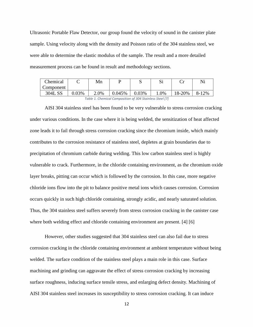
AISI 304 stainless steel has high strength and corrosion resistance. It is mainly composed
of chromium, which contributes to its corrosion resistance, and nickel, which mainly contributes
to its strength. Its chemical composition can be found in Table 1 below. By using GE USN 60
12
Ultrasonic Portable Flaw Detector, our group found the velocity of sound in the canister plate
sample. Using velocity along with the density and Poisson ratio of the 304 stainless steel, we
were able to determine the elastic modulus of the sample. The result and a more detailed
measurement process can be found in result and methodology sections.
Chemical
Component
C Mn P S Si Cr Ni
304L SS 0.03% 2.0% 0.045% 0.03% 1.0% 18-20% 8-12% Table 1. Chemical Composition of 304 Stainless Steel [7]
AISI 304 stainless steel has been found to be very vulnerable to stress corrosion cracking
under various conditions. In the case where it is being welded, the sensitization of heat affected
zone leads it to fail through stress corrosion cracking since the chromium inside, which mainly
contributes to the corrosion resistance of stainless steel, depletes at grain boundaries due to
precipitation of chromium carbide during welding. This low carbon stainless steel is highly
vulnerable to crack. Furthermore, in the chloride containing environment, as the chromium oxide
layer breaks, pitting can occur which is followed by the corrosion. In this case, more negative
chloride ions flow into the pit to balance positive metal ions which causes corrosion. Corrosion
occurs quickly in such high chloride containing, strongly acidic, and nearly saturated solution.
Thus, the 304 stainless steel suffers severely from stress corrosion cracking in the canister case
where both welding effect and chloride containing environment are present. [4] [6]
However, other studies suggested that 304 stainless steel can also fail due to stress
corrosion cracking in the chloride containing environment at ambient temperature without being
welded. The surface condition of the stainless steel plays a main role in this case. Surface
machining and grinding can aggravate the effect of stress corrosion cracking by increasing
surface roughness, inducing surface tensile stress, and enlarging defect density. Machining of
AISI 304 stainless steel increases its susceptibility to stress corrosion cracking. It can induce
13
surface plastic strain and deformation which result in the transformation of austenite matrix near
the surface into martensite. Such transformation results in a large amount of work-hardening of
the material. The work hardened layers cause the material to crack much faster in the chloride
solution. Since the canister plates were grinded for surface cleaning once welding was done, the
surface deformation by such machining requires a closer attention when characterizing residual
stress. [8]
Contour Method
The contour method involves in cutting specimen into two pieces and measuring the
structural deformation on the cut planes after residual stress has been relieved. The measured
deformation data is being input to a finite element model to calculate residual stress at the
surface of the specimen before cut. In the finite element model, the deformation data is imposed
as a set of displacement boundary conditions on the model. The model accounts for material
properties and geometry of the specimen as well as thermo data during the measurement to
produce a comprehensive calculation of the residual stress. Specimens used for contour method
are typically metals and they are being cut by electric discharge machining (EDM) method which
induces minimum cutting stress. [9]
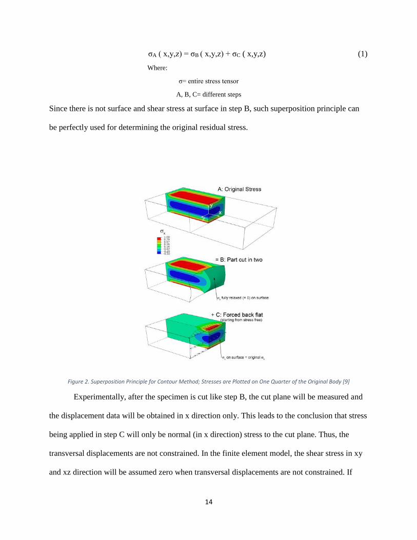
The contour method follows a superposition principle as shown in Figure 2. The step A
shows the original one quarter of uncut specimen with residual stress in the structure. In step B,
the specimen is cut in half at x=0 and the residual stress is being released. In step C, stress is
being applied on cut surface and forces it back to its original shape like in step A. The amount of
such applied stress is the amount of the residual stress that exists in the original specimen. This
step is typically done by using the finite element model. [9]Steps mentioned above can be also
described by Equation 2 in the following:
14
σA ( x,y,z) = σB ( x,y,z) + σC ( x,y,z) (1)
Where:
σ= entire stress tensor
A, B, C= different steps
Since there is not surface and shear stress at surface in step B, such superposition principle can
be perfectly used for determining the original residual stress.
Figure 2. Superposition Principle for Contour Method; Stresses are Plotted on One Quarter of the Original Body [9]
Experimentally, after the specimen is cut like step B, the cut plane will be measured and
the displacement data will be obtained in x direction only. This leads to the conclusion that stress
being applied in step C will only be normal (in x direction) stress to the cut plane. Thus, the
transversal displacements are not constrained. In the finite element model, the shear stress in xy
and xz direction will be assumed zero when transversal displacements are not constrained. If
15
there is any shear stress or transversal displacement appears, averaging two cut contours can
cancel them out which results in only normal displacement exists at the cut plane. [9]
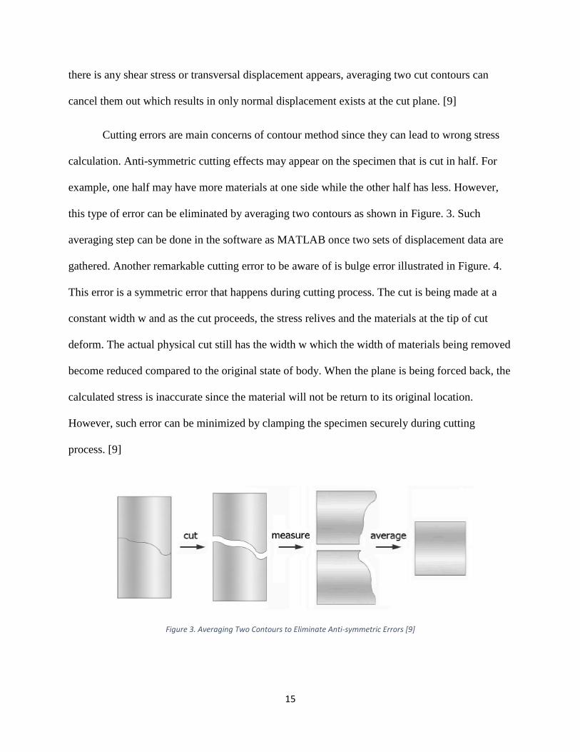
Cutting errors are main concerns of contour method since they can lead to wrong stress
calculation. Anti-symmetric cutting effects may appear on the specimen that is cut in half. For
example, one half may have more materials at one side while the other half has less. However,
this type of error can be eliminated by averaging two contours as shown in Figure. 3. Such
averaging step can be done in the software as MATLAB once two sets of displacement data are
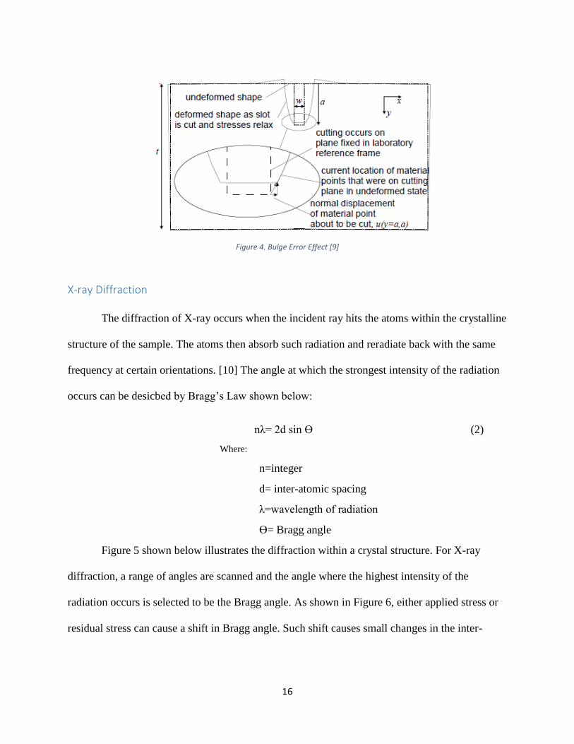
gathered. Another remarkable cutting error to be aware of is bulge error illustrated in Figure. 4.
This error is a symmetric error that happens during cutting process. The cut is being made at a
constant width w and as the cut proceeds, the stress relives and the materials at the tip of cut
deform. The actual physical cut still has the width w which the width of materials being removed
become reduced compared to the original state of body. When the plane is being forced back, the
calculated stress is inaccurate since the material will not be return to its original location.
However, such error can be minimized by clamping the specimen securely during cutting
process. [9]
Figure 3. Averaging Two Contours to Eliminate Anti-symmetric Errors [9]
16
X-ray Diffraction
The diffraction of X-ray occurs when the incident ray hits the atoms within the crystalline
structure of the sample. The atoms then absorb such radiation and reradiate back with the same
frequency at certain orientations. [10] The angle at which the strongest intensity of the radiation
occurs can be desicbed by Bragg’s Law shown below:
nλ= 2d sin ϴ (2)
Where:
n=integer
d= inter-atomic spacing
λ=wavelength of radiation
ϴ= Bragg angle
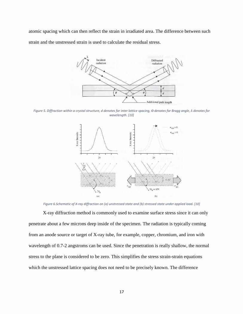
Figure 5 shown below illustrates the diffraction within a crystal structure. For X-ray
diffraction, a range of angles are scanned and the angle where the highest intensity of the
radiation occurs is selected to be the Bragg angle. As shown in Figure 6, either applied stress or
residual stress can cause a shift in Bragg angle. Such shift causes small changes in the inter-
Figure 4. Bulge Error Effect [9]
17
atomic spacing which can then reflect the strain in irradiated area. The difference between such
strain and the unstressed strain is used to calculate the residual stress.
Figure 5. Diffraction within a crystal structure, d denotes for inter lattice spacing, ϴ denotes for Bragg angle, λ denotes for wavelength. [10]
Figure 6.Schematic of X-ray diffraction on (a) unstressed state and (b) stressed state under applied load. [10]
X-ray diffraction method is commonly used to examine surface stress since it can only
penetrate about a few microns deep inside of the specimen. The radiation is typically coming
from an anode source or target of X-ray tube, for example, copper, chromium, and iron with
wavelength of 0.7-2 angstroms can be used. Since the penetration is really shallow, the normal
stress to the plane is considered to be zero. This simplifies the stress strain-strain equations
which the unstressed lattice spacing does not need to be precisely known. The difference
18
between specific lattice planes at several angles to the surface plane can be used to extrapolate
the strain condition to a vector in the plane of the surface. [10]
Two techniques can be used to measure strain and stress through X-ray diffraction [10]:
1. Determining the elastic strain by measuring the atomic lattice spacing along
different orientations using a diffractometer. These strains then undergo the
transformation law for second rank tensors to compute strain tensors in the
specimen coordinate. The stresses can then be calculated through Hooke’s Law.
This technique can be used in either single crystal structures or polycrystalline
structures.
2. Determining the local and global curvatures of single-crystal sample through
tracking the orientation of a crystal direction as a function of position within the
sample using a goniometer equipped with a translation gage. If these curvatures are
caused by the elastic constraints within the sample, the stresses can be calculated by
using various formulas such as the Stoney Formula.
Neutron Diffraction Method
Neutron diffraction method also uses radiation penetrating technique to measure
deformed strains caused by residual stress. Unlike in X-ray diffraction which the radiation
interacts with the atoms in the crystal structure, in neutron diffraction, the neutrons are emitted to
interact directly with the nucleus of the atoms. The diffracted intensity interacts with the
electrons. Neutron diffraction also allows the radiation to penetrate in cm range deep inside the
material which bulk stress can be measured. Neutrons are generally produced from fission or
spallation and neutron energy usually provides 0.3 to 7 Angstroms for wavelength. Neutron
19
diffraction allows the measurement of residual stress of samples that can have 0.1-1.5m
thickness with a spatial resolution less than 1 mm which it does not require materials removal
from the samples. Compare to X-ray diffraction method, neutron diffraction method also uses
Bragg angle to calculate lattice spacing. The difference in lattice spacing indicates the change in
strain which the residual stress can be calculated. However, neutron diffraction provides
measurement of 3-dimensional stress which the unstressed lattice spacing must be precisely
known. [11]
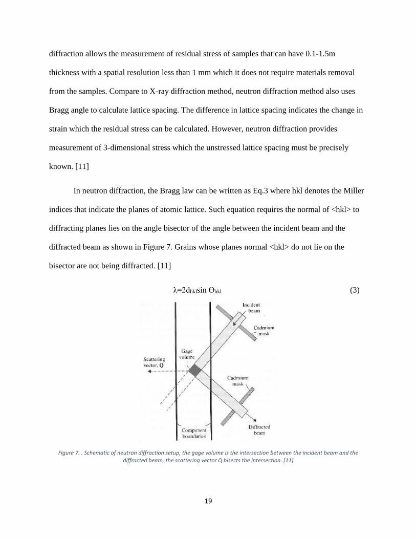
In neutron diffraction, the Bragg law can be written as Eq.3 where hkl denotes the Miller
indices that indicate the planes of atomic lattice. Such equation requires the normal of <hkl> to
diffracting planes lies on the angle bisector of the angle between the incident beam and the
diffracted beam as shown in Figure 7. Grains whose planes normal <hkl> do not lie on the
bisector are not being diffracted. [11]
λ=2dhklsin ϴhkl (3)
Figure 7. . Schematic of neutron diffraction setup, the gage volume is the intersection between the incident beam and the diffracted beam, the scattering vector Q bisects the intersection. [11]
20
Hole Drilling Method
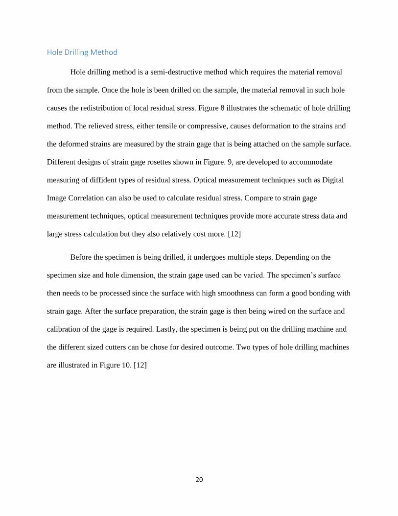
Hole drilling method is a semi-destructive method which requires the material removal
from the sample. Once the hole is been drilled on the sample, the material removal in such hole
causes the redistribution of local residual stress. Figure 8 illustrates the schematic of hole drilling
method. The relieved stress, either tensile or compressive, causes deformation to the strains and
the deformed strains are measured by the strain gage that is being attached on the sample surface.
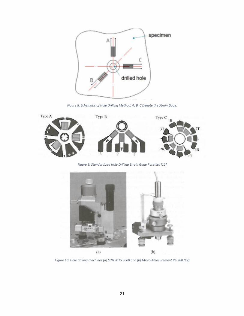
Different designs of strain gage rosettes shown in Figure. 9, are developed to accommodate
measuring of diffident types of residual stress. Optical measurement techniques such as Digital
Image Correlation can also be used to calculate residual stress. Compare to strain gage
measurement techniques, optical measurement techniques provide more accurate stress data and
large stress calculation but they also relatively cost more. [12]
Before the specimen is being drilled, it undergoes multiple steps. Depending on the
specimen size and hole dimension, the strain gage used can be varied. The specimen’s surface
then needs to be processed since the surface with high smoothness can form a good bonding with
strain gage. After the surface preparation, the strain gage is then being wired on the surface and
calibration of the gage is required. Lastly, the specimen is being put on the drilling machine and
the different sized cutters can be chose for desired outcome. Two types of hole drilling machines
are illustrated in Figure 10. [12]
21
Figure 8. Schematic of Hole Drilling Method, A, B, C Denote the Strain Gage.
Figure 9. Standardized Hole Drilling Strain Gage Rosettes [12]
Figure 10. Hole drilling machines (a) SINT MTS 3000 and (b) Micro-Measurement RS-200 [12]
22
Methodology
Various material properties were characterized for the stainless steel samples for better
understanding of the materials and accurate stress calculation.
Young’s Modulus
In order to compare and confirm results with parallel tensile testing, we wanted to
measure the Young’s Modulus of the stainless steel sample by another method. The acoustic
method where the Young’s Modulus of the material is calculated from density, poisson ratio and
the velocity of sound in the material was selected. The velocity of sound in a material is
influenced by many factors including the Young’s modulus of the material, which means that the
Young’s modulus of a material can be calculated if given the velocity of sound in that material.
The Young’s modulus is given by
E = 𝑉2𝜌(1+𝑣)(1−2𝑣)
1−𝑣
Where V is the velocity of sound, 𝜌 is the density of material and v is the Poisson ratio of
the material. For this measurement, both 𝜌 and v are taken from literature that 𝜌=7778kgm-3 and
v=0.27.
The velocity of sound in the material is measured by GE USN 60 Ultrasonic Portable
Flaw Detector, Krautkramer. A single element probe N5198 of frequency 10MHz was used in
couple. The auto calibration feature of USN 60 was used to calculate velocity of sound and the
values obtained are readings displayed on USN 60. Two pieces of sample of same stainless steel
but with different thickness were required for such calibration. Their thicknesses were measured
with a Vernier Caliper (0.001 inch). Calibration was performed five times and the average of the
velocity of sound was 5740±4ms-1.
(4)
23
Macro and Micro Hardness
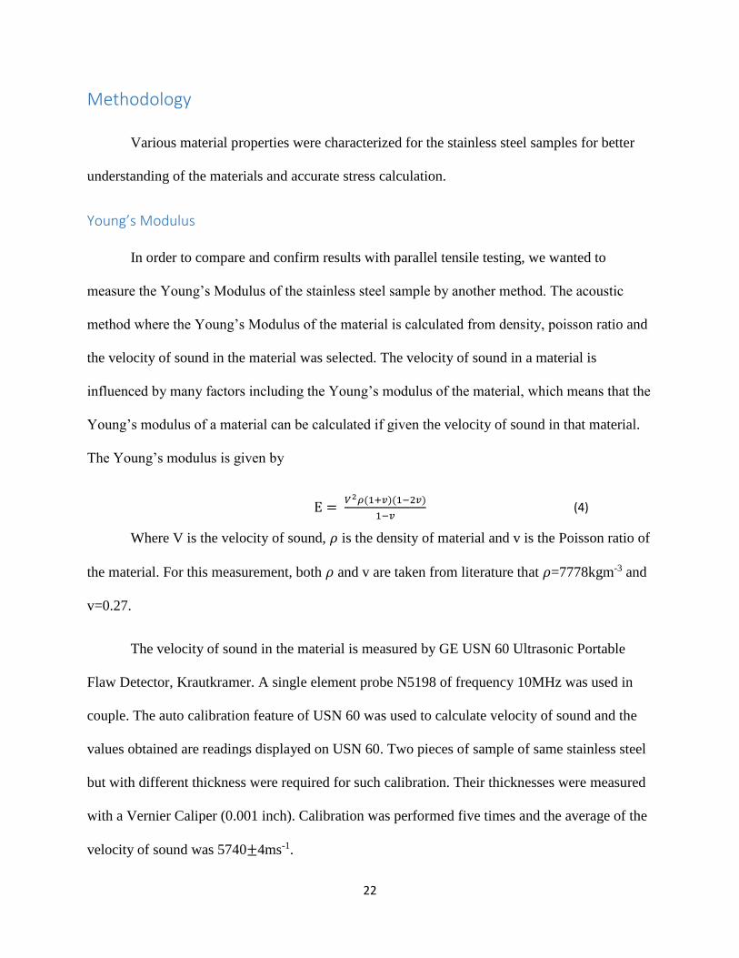
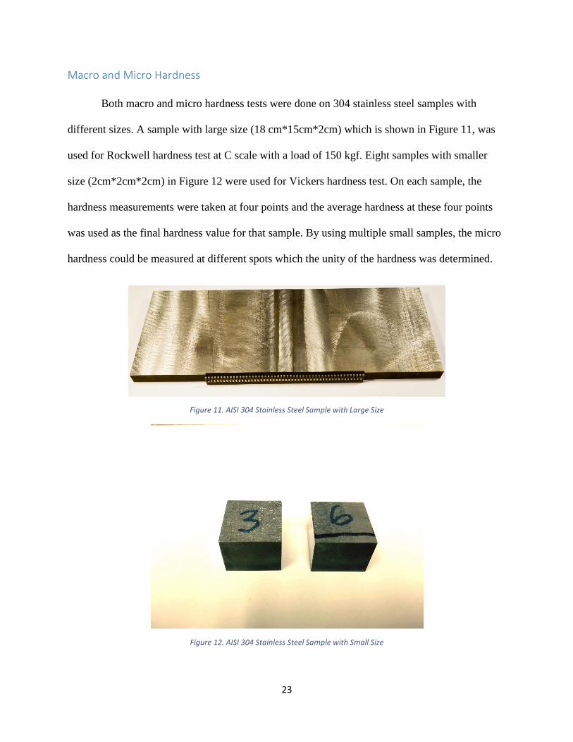
Both macro and micro hardness tests were done on 304 stainless steel samples with
different sizes. A sample with large size (18 cm*15cm*2cm) which is shown in Figure 11, was
used for Rockwell hardness test at C scale with a load of 150 kgf. Eight samples with smaller
size (2cm*2cm*2cm) in Figure 12 were used for Vickers hardness test. On each sample, the
hardness measurements were taken at four points and the average hardness at these four points
was used as the final hardness value for that sample. By using multiple small samples, the micro
hardness could be measured at different spots which the unity of the hardness was determined.
Figure 11. AISI 304 Stainless Steel Sample with Large Size
Figure 12. AISI 304 Stainless Steel Sample with Small Size
24
Microstructure
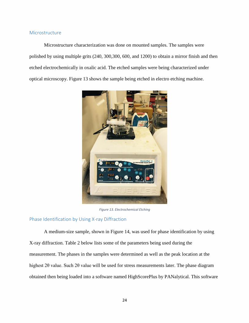
Microstructure characterization was done on mounted samples. The samples were
polished by using multiple grits (240, 300,300, 600, and 1200) to obtain a mirror finish and then
etched electrochemically in oxalic acid. The etched samples were being characterized under
optical microscopy. Figure 13 shows the sample being etched in electro etching machine.
Figure 13. Electrochemical Etching
Phase Identification by Using X-ray Diffraction
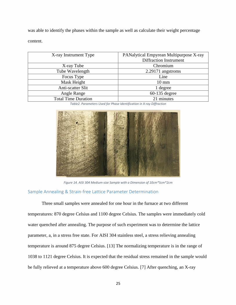
A medium-size sample, shown in Figure 14, was used for phase identification by using
X-ray diffraction. Table 2 below lists some of the parameters being used during the
measurement. The phases in the samples were determined as well as the peak location at the
highest 2θ value. Such 2θ value will be used for stress measurements later. The phase diagram
obtained then being loaded into a software named HighScorePlus by PANalytical. This software
25
was able to identify the phases within the sample as well as calculate their weight percentage
content.
X-ray Instrument Type PANalytical Empyrean Multipurpose X-ray
Diffraction Instrument
X-ray Tube Chromium
Tube Wavelength 2.29171 angstroms
Focus Type Line
Mask Height 10 mm
Anti-scatter Slit 1 degree
Angle Range 60-135 degree
Total Time Duration 21 minutes Table2. Parameters Used for Phase Identification in X-ray Diffraction
Figure 14. AISI 304 Medium-size Sample with a Dimension of 10cm*5cm*2cm
Sample Annealing & Strain-free Lattice Parameter Determination
Three small samples were annealed for one hour in the furnace at two different
temperatures: 870 degree Celsius and 1100 degree Celsius. The samples were immediately cold
water quenched after annealing. The purpose of such experiment was to determine the lattice
parameter, a, in a stress free state. For AISI 304 stainless steel, a stress relieving annealing
temperature is around 875 degree Celsius. [13] The normalizing temperature is in the range of
1038 to 1121 degree Celsius. It is expected that the residual stress remained in the sample would
be fully relieved at a temperature above 600 degree Celsius. [7] After quenching, an X-ray
26
diffraction analysis was done on all samples with the same parameters listed in Table 2 above.
Once the highest peak location was determined for all samples, the Bragg Law which was shown
in Eq. 2, was used to calculate d-spacing. Once the d-spacing values were obtained, the strain-
free lattice parameter could be obtained from Eq.5.
(5)
Where:
d= d-spacing
a= lattice parameter
h,k,l= Miller Indices
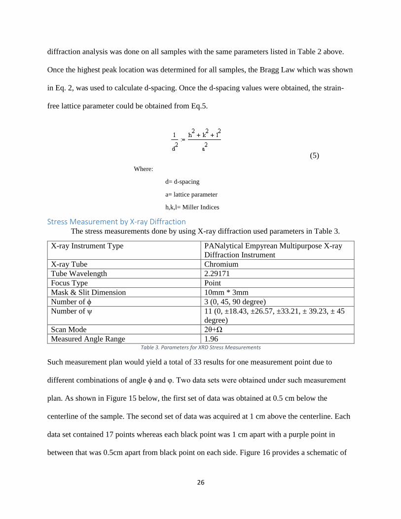
Stress Measurement by X-ray Diffraction The stress measurements done by using X-ray diffraction used parameters in Table 3.
X-ray Instrument Type PANalytical Empyrean Multipurpose X-ray
Diffraction Instrument
X-ray Tube Chromium
Tube Wavelength 2.29171
Focus Type Point
Mask & Slit Dimension 10mm * 3mm
Number of ϕ 3 (0, 45, 90 degree)
Number of ψ 11 (0, ±18.43, ±26.57, ±33.21, ± 39.23, ± 45
degree)
Scan Mode 2θ+Ω
Measured Angle Range 1.96 Table 3. Parameters for XRD Stress Measurements
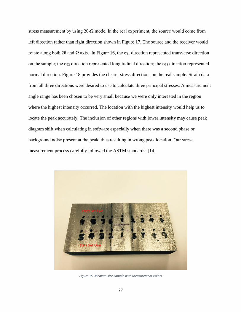
Such measurement plan would yield a total of 33 results for one measurement point due to
different combinations of angle ϕ and φ. Two data sets were obtained under such measurement
plan. As shown in Figure 15 below, the first set of data was obtained at 0.5 cm below the
centerline of the sample. The second set of data was acquired at 1 cm above the centerline. Each
data set contained 17 points whereas each black point was 1 cm apart with a purple point in
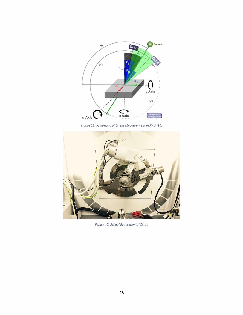
between that was 0.5cm apart from black point on each side. Figure 16 provides a schematic of
27
stress measurement by using 2θ-Ω mode. In the real experiment, the source would come from
left direction rather than right direction shown in Figure 17. The source and the receiver would
rotate along both 2θ and Ω axis. In Figure 16, the σ11 direction represented transverse direction
on the sample; the σ22 direction represented longitudinal direction; the σ33 direction represented
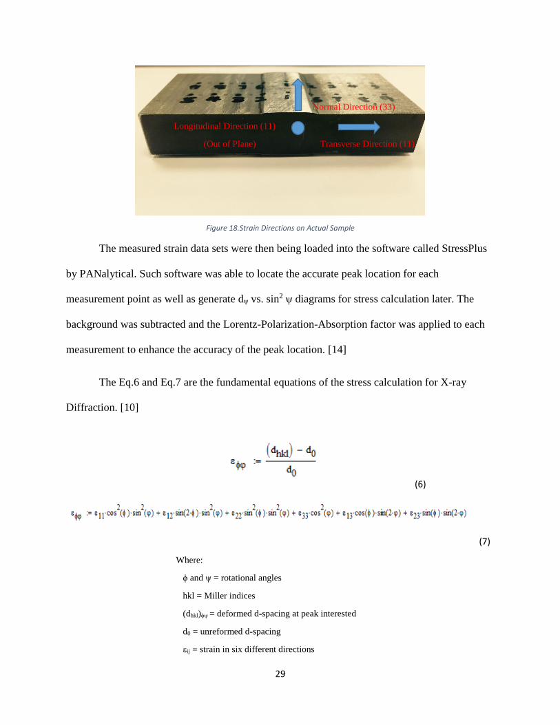
normal direction. Figure 18 provides the clearer stress directions on the real sample. Strain data
from all three directions were desired to use to calculate three principal stresses. A measurement
angle range has been chosen to be very small because we were only interested in the region
where the highest intensity occurred. The location with the highest intensity would help us to
locate the peak accurately. The inclusion of other regions with lower intensity may cause peak
diagram shift when calculating in software especially when there was a second phase or
background noise present at the peak, thus resulting in wrong peak location. Our stress
measurement process carefully followed the ASTM standards. [14]
Figure 15. Medium-size Sample with Measurement Points
Data Set One
Data Set Two
28
Figure 16. Schematic of Stress Measurement in XRD [14]
Figure 17. Actual Experimental Setup
29
Figure 18.Strain Directions on Actual Sample
The measured strain data sets were then being loaded into the software called StressPlus
by PANalytical. Such software was able to locate the accurate peak location for each
measurement point as well as generate dψ vs. sin2 ψ diagrams for stress calculation later. The
background was subtracted and the Lorentz-Polarization-Absorption factor was applied to each
measurement to enhance the accuracy of the peak location. [14]
The Eq.6 and Eq.7 are the fundamental equations of the stress calculation for X-ray
Diffraction. [10]
(6)
(7)
Where:
ϕ and ψ = rotational angles
hkl = Miller indices
(dhkl)ϕψ = deformed d-spacing at peak interested
d0 = unreformed d-spacing
εij = strain in six different directions
Transverse Direction (11)
Normal Direction (33)
Longitudinal Direction (11)
(Out of Plane)
30
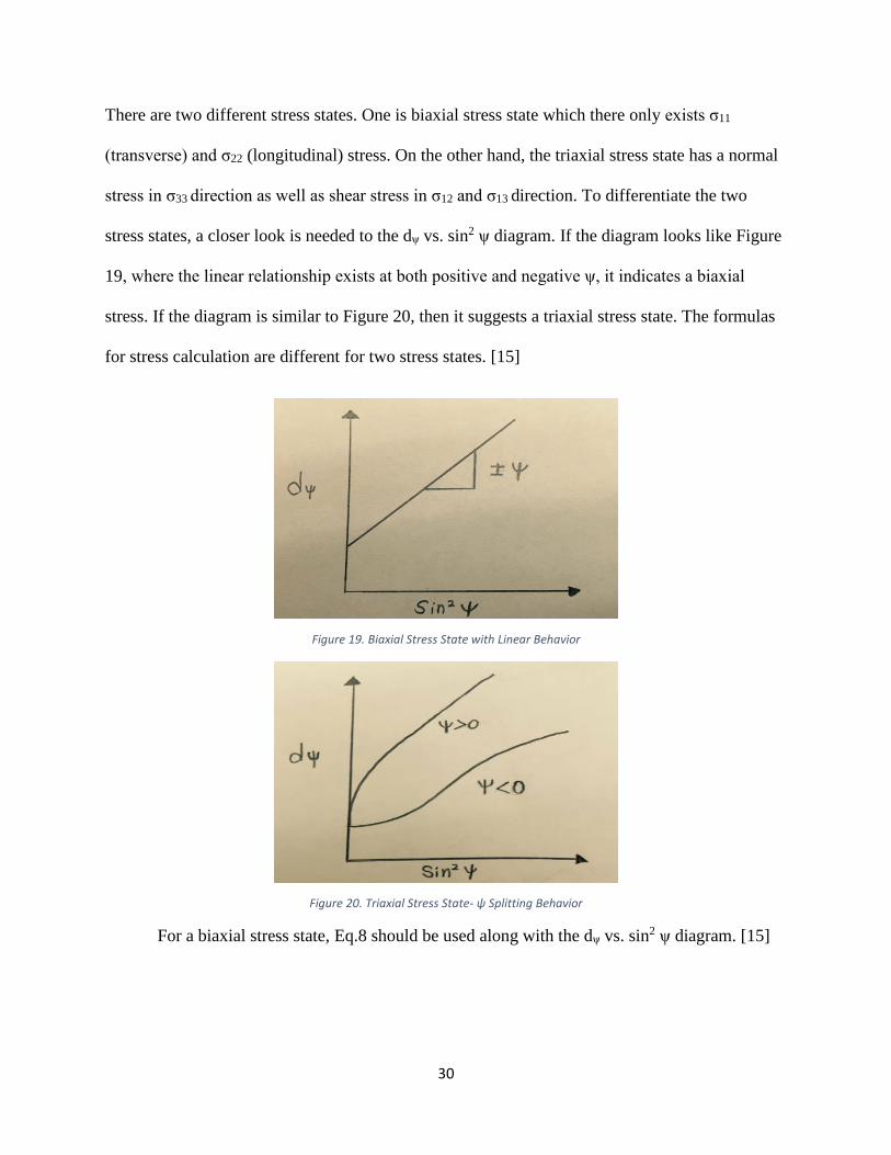
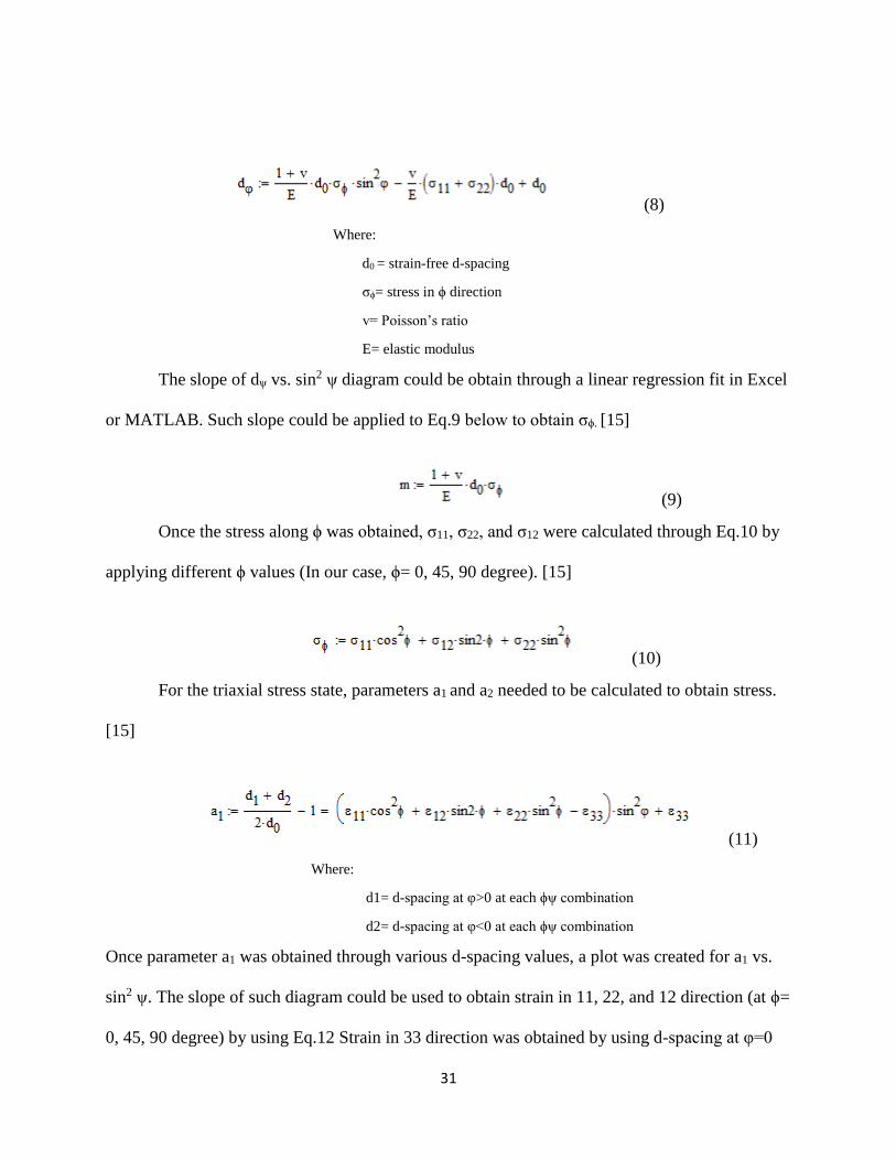
There are two different stress states. One is biaxial stress state which there only exists σ11
(transverse) and σ22 (longitudinal) stress. On the other hand, the triaxial stress state has a normal
stress in σ33 direction as well as shear stress in σ12 and σ13 direction. To differentiate the two
stress states, a closer look is needed to the dψ vs. sin2 ψ diagram. If the diagram looks like Figure
19, where the linear relationship exists at both positive and negative ψ, it indicates a biaxial
stress. If the diagram is similar to Figure 20, then it suggests a triaxial stress state. The formulas
for stress calculation are different for two stress states. [15]
Figure 19. Biaxial Stress State with Linear Behavior
Figure 20. Triaxial Stress State- ψ Splitting Behavior
For a biaxial stress state, Eq.8 should be used along with the dψ vs. sin2 ψ diagram. [15]
31
(8)
Where:
d0 = strain-free d-spacing
σϕ= stress in ϕ direction
v= Poisson’s ratio
E= elastic modulus
The slope of dψ vs. sin2 ψ diagram could be obtain through a linear regression fit in Excel
or MATLAB. Such slope could be applied to Eq.9 below to obtain σϕ. [15]
(9)
Once the stress along ϕ was obtained, σ11, σ22, and σ12 were calculated through Eq.10 by
applying different ϕ values (In our case, ϕ= 0, 45, 90 degree). [15]
(10)
For the triaxial stress state, parameters a1 and a2 needed to be calculated to obtain stress.
[15]
(11)
Where:
d1= d-spacing at φ>0 at each ϕψ combination
d2= d-spacing at φ<0 at each ϕψ combination
Once parameter a1 was obtained through various d-spacing values, a plot was created for a1 vs.
sin2 ψ. The slope of such diagram could be used to obtain strain in 11, 22, and 12 direction (at ϕ=
0, 45, 90 degree) by using Eq.12 Strain in 33 direction was obtained by using d-spacing at φ=0
32
and ϕ= 0, 45, 90. Note that all three d-spacing values at φ=0 should be the same and such
phenomenon would indicate if any misalignments of the instrument exist in the system. [15]
(12)
Parameter a2 could be generated by using Eq. 13. [15]
(13)
Once a2 was obtained from Eq.13, a plot was created for a2 vs. sin |2𝜑|. The sloped was
extracted from the linear fitted line and it could be applied to Eq.14 to obtain shear strains in 12
direction (ϕ=0) and 23 direction (ϕ=90). [15]
(14)
All strains acquired were used to calculate stress in different directions by multiplying them with
elastic modulus and one plus Poisson ratio.
Results and Discussion
Elastic Modulus
According to Eq.1 the E was calculated to be 205GPa. Assuming ρ and v were exact
values, the error involved in measurement is about 0.1%.
Macro and Micro Hardness
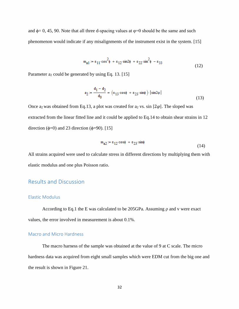
The macro harness of the sample was obtained at the value of 9 at C scale. The micro
hardness data was acquired from eight small samples which were EDM cut from the big one and
the result is shown in Figure 21.
33
Figure 21. Micro Hardness on Eight Small Samples
According to both hardness results, it has been confirmed that the stainless steel samples have
been annealed which the materials were really soft.
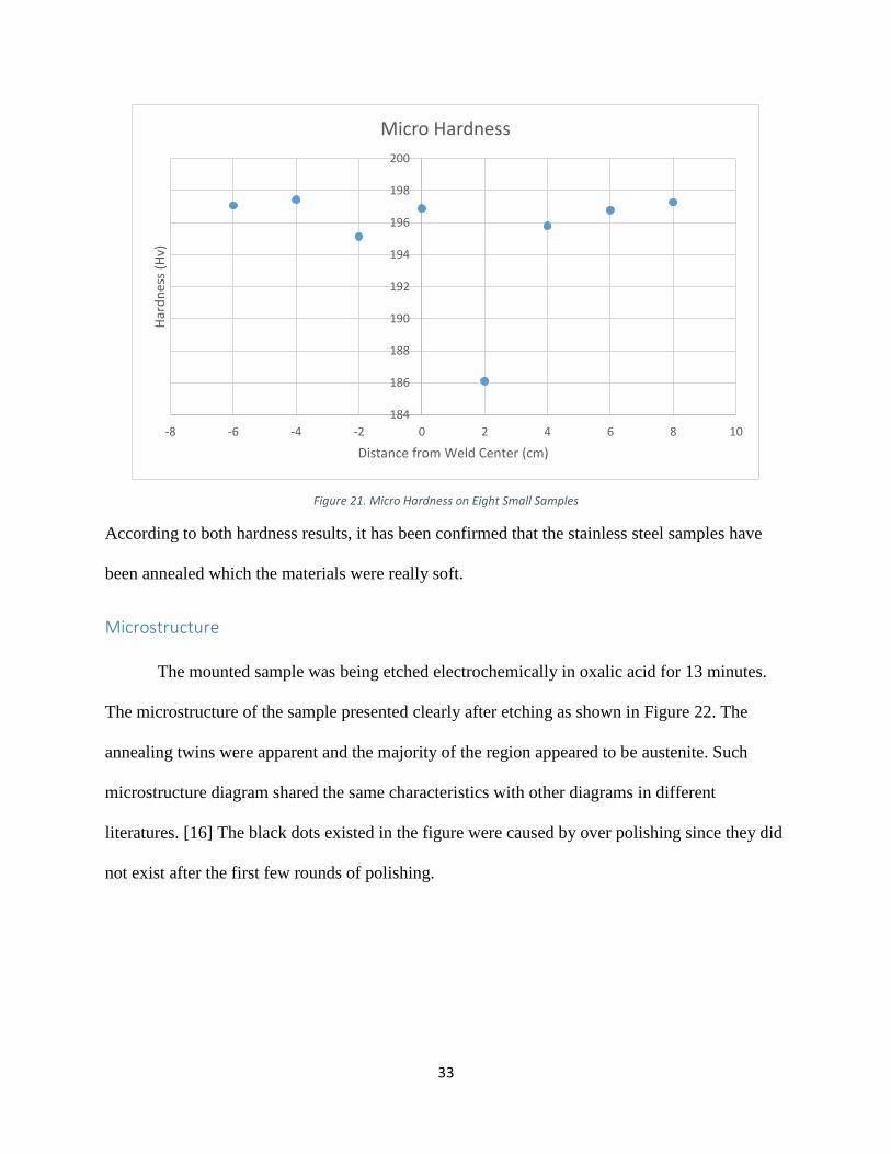
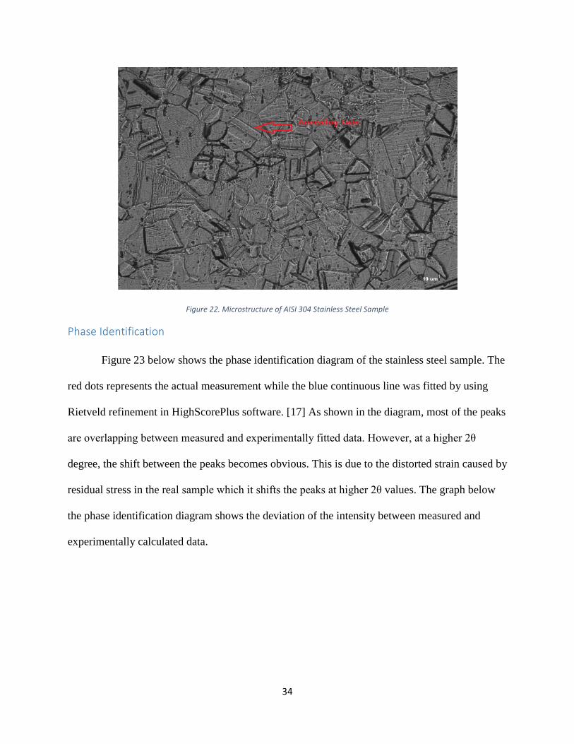
Microstructure
The mounted sample was being etched electrochemically in oxalic acid for 13 minutes.
The microstructure of the sample presented clearly after etching as shown in Figure 22. The
annealing twins were apparent and the majority of the region appeared to be austenite. Such
microstructure diagram shared the same characteristics with other diagrams in different
literatures. [16] The black dots existed in the figure were caused by over polishing since they did
not exist after the first few rounds of polishing.
184
186
188
190
192
194
196
198
200
-8 -6 -4 -2 0 2 4 6 8 10
Har
dn
ess
(Hv)
Distance from Weld Center (cm)
Micro Hardness
34
Figure 22. Microstructure of AISI 304 Stainless Steel Sample
Phase Identification
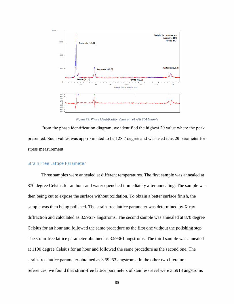
Figure 23 below shows the phase identification diagram of the stainless steel sample. The
red dots represents the actual measurement while the blue continuous line was fitted by using
Rietveld refinement in HighScorePlus software. [17] As shown in the diagram, most of the peaks
are overlapping between measured and experimentally fitted data. However, at a higher 2θ
degree, the shift between the peaks becomes obvious. This is due to the distorted strain caused by
residual stress in the real sample which it shifts the peaks at higher 2θ values. The graph below
the phase identification diagram shows the deviation of the intensity between measured and
experimentally calculated data.
35
Figure 23. Phase Identification Diagram of AISI 304 Sample
From the phase identification diagram, we identified the highest 2θ value where the peak
presented. Such values was approximated to be 128.7 degree and was used it as 2θ parameter for
stress measurement.
Strain Free Lattice Parameter
Three samples were annealed at different temperatures. The first sample was annealed at
870 degree Celsius for an hour and water quenched immediately after annealing. The sample was
then being cut to expose the surface without oxidation. To obtain a better surface finish, the
sample was then being polished. The strain-free lattice parameter was determined by X-ray
diffraction and calculated as 3.59617 angstroms. The second sample was annealed at 870 degree
Celsius for an hour and followed the same procedure as the first one without the polishing step.
The strain-free lattice parameter obtained as 3.59361 angstroms. The third sample was annealed
at 1100 degree Celsius for an hour and followed the same procedure as the second one. The
strain-free lattice parameter obtained as 3.59253 angstroms. In the other two literature
references, we found that strain-free lattice parameters of stainless steel were 3.5918 angstroms
36
and 3.6114 angstroms. Due to slightly chemical component difference and various machining
processes for different stainless steel samples, it was safe to assume that any strain-free
parameters in the range of 3.5918 to 3.6114 were acceptable for AISI 304 stainless steel. All
three measured values fell into this range but we preferred the second and third value since
polishing may induce some stress to the sample. Table 4 lists the d-spacing values with their
respective lattice parameters.
A( lattice parameter, angstroms) D0 (strain-free d-spacing, angstroms)
3.59617 (annealed @880 C, polished) 1.27189
3.59361(annealed @ 880C) 1.27053
3.59253 (annealed @ 1100C) 1.27015
3.5918 1.26989
3.6114 1.27682 Table 4. D-spacing Values with Their Respective Strain-free Lattice Parameters
For the stress calculation in this project, the values of d0 were chose to be 1.27053 for data set
one and 1.27015 for data set two.
Stress Calculation
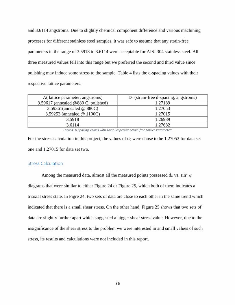
Among the measured data, almost all the measured points possessed dψ vs. sin2 ψ
diagrams that were similar to either Figure 24 or Figure 25, which both of them indicates a
triaxial stress state. In Figre 24, two sets of data are close to each other in the same trend which
indicated that there is a small shear stress. On the other hand, Figure 25 shows that two sets of
data are slightly further apart which suggested a bigger shear stress value. However, due to the
insignificance of the shear stress to the problem we were interested in and small values of such
stress, its results and calculations were not included in this report.
37
(a) (b)
Normal Stress
Normal stress plays an important role in determining transverse stress and longitudinal
stress according to Eq. 15. It is the formula for calculating normal strain.
(15)
In this formula, three dϕφ were measured at φ=0 and ϕ=0, 45, 90. All three values should be the
same or varied slightly to check if the instruments have any errors. [10]
Stress Measurements
Set One
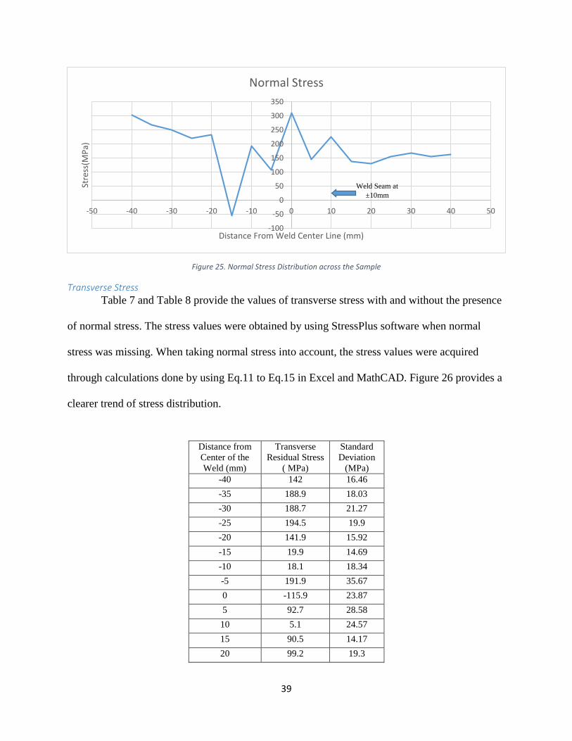
Normal Stress
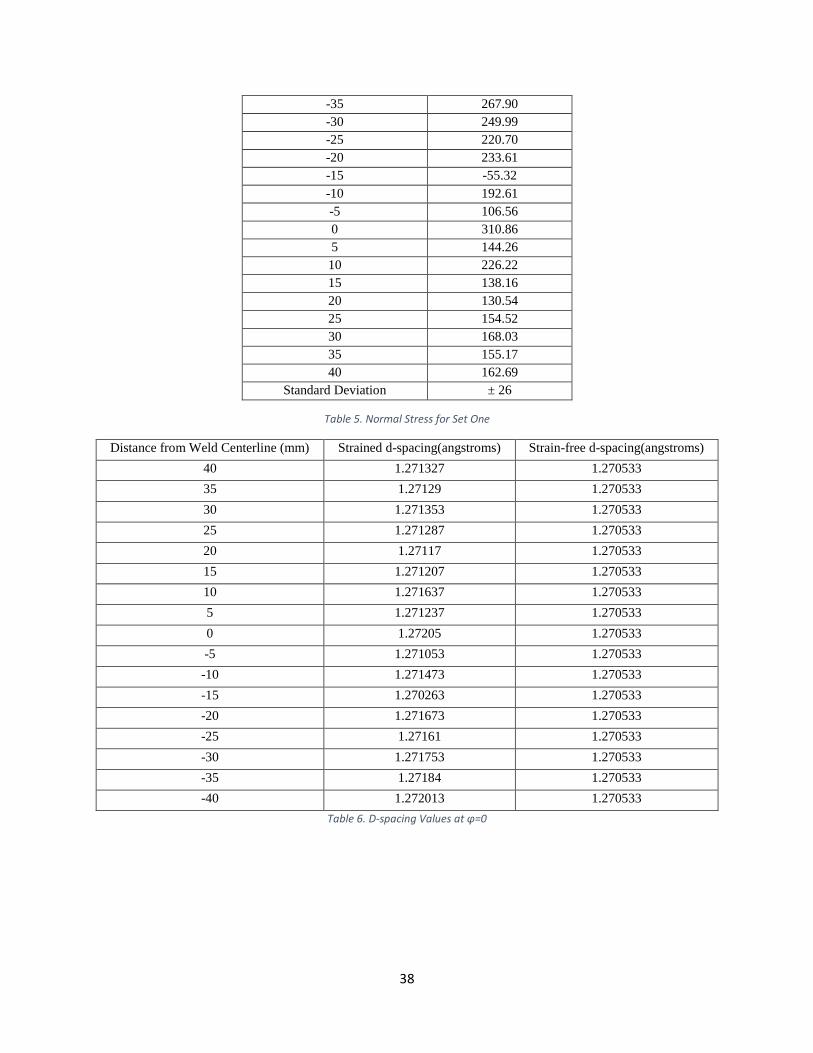
Table 5 includes the value of normal stress at each measured point. Figure 25 provides a
clearer trend of normal stress across the sample. The strain free d-spacing value used was
1.270533 for stress calculations in all three directions. Table 6 includes d-spacing values
measured at φ=0 for normal stress calculation.
Distance from Center of the
Weld (mm)
Normal Residual Stress
( MPa)
-40 303.30
Figure 24. (a) Linear Behavior with Small Shear Stress; (b) ψ Splitting Behavior with Larger Shear Stress (triangle indicates data measured at positive ψ and square indicates data measured at negative ψ)
38
Table 5. Normal Stress for Set One
Distance from Weld Centerline (mm) Strained d-spacing(angstroms) Strain-free d-spacing(angstroms)
40 1.271327 1.270533
35 1.27129 1.270533
30 1.271353 1.270533
25 1.271287 1.270533
20 1.27117 1.270533
15 1.271207 1.270533
10 1.271637 1.270533
5 1.271237 1.270533
0 1.27205 1.270533
-5 1.271053 1.270533
-10 1.271473 1.270533
-15 1.270263 1.270533
-20 1.271673 1.270533
-25 1.27161 1.270533
-30 1.271753 1.270533
-35 1.27184 1.270533
-40 1.272013 1.270533
Table 6. D-spacing Values at φ=0
-35 267.90
-30 249.99
-25 220.70
-20 233.61
-15 -55.32
-10 192.61
-5 106.56
0 310.86
5 144.26
10 226.22
15 138.16
20 130.54
25 154.52
30 168.03
35 155.17
40 162.69
Standard Deviation ± 26
39
Figure 25. Normal Stress Distribution across the Sample
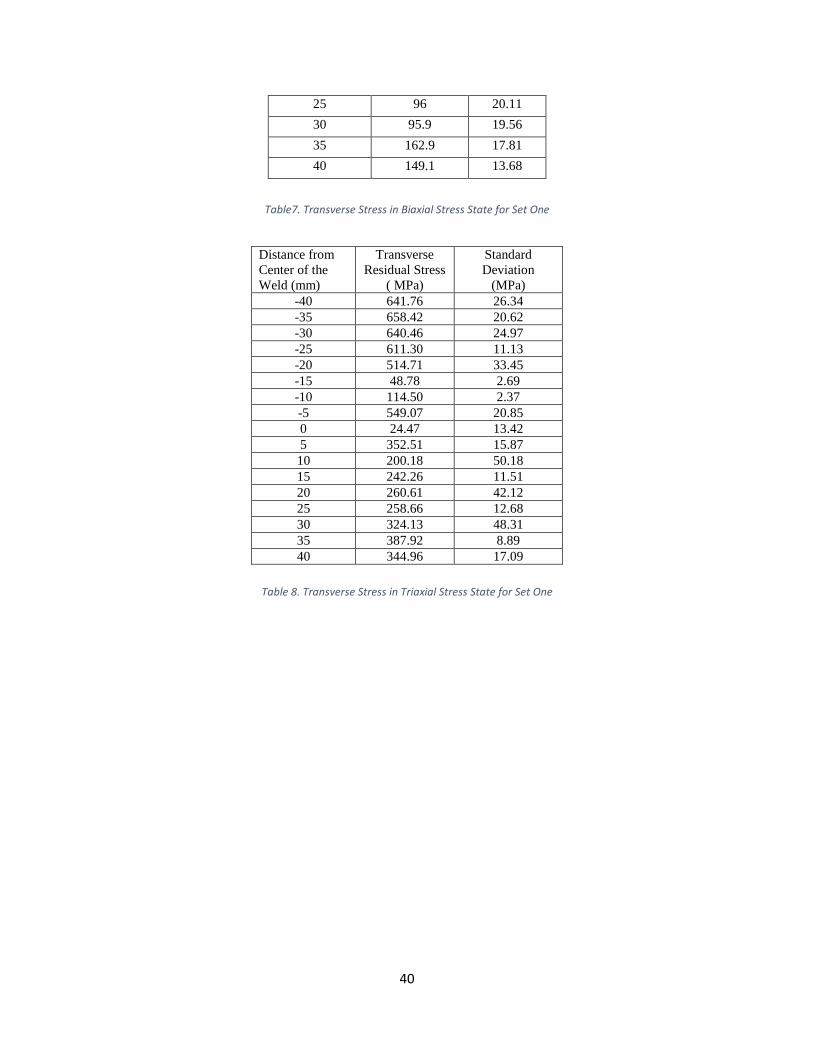
Transverse Stress
Table 7 and Table 8 provide the values of transverse stress with and without the presence
of normal stress. The stress values were obtained by using StressPlus software when normal
stress was missing. When taking normal stress into account, the stress values were acquired
through calculations done by using Eq.11 to Eq.15 in Excel and MathCAD. Figure 26 provides a
clearer trend of stress distribution.
-100
-50
0
50
100
150
200
250
300
350
-50 -40 -30 -20 -10 0 10 20 30 40 50
Stre
ss(M
Pa)
Distance From Weld Center Line (mm)
Normal Stress
Distance from
Center of the
Weld (mm)
Transverse
Residual Stress
( MPa)
Standard
Deviation
(MPa)
-40 142 16.46
-35 188.9 18.03
-30 188.7 21.27
-25 194.5 19.9
-20 141.9 15.92
-15 19.9 14.69
-10 18.1 18.34
-5 191.9 35.67
0 -115.9 23.87
5 92.7 28.58
10 5.1 24.57
15 90.5 14.17
20 99.2 19.3
Weld Seam at
±10mm
40
Table7. Transverse Stress in Biaxial Stress State for Set One
Table 8. Transverse Stress in Triaxial Stress State for Set One
25 96 20.11
30 95.9 19.56
35 162.9 17.81
40 149.1 13.68
Distance from
Center of the
Weld (mm)
Transverse
Residual Stress
( MPa)
Standard
Deviation
(MPa)
-40 641.76 26.34
-35 658.42 20.62
-30 640.46 24.97
-25 611.30 11.13
-20 514.71 33.45
-15 48.78 2.69
-10 114.50 2.37
-5 549.07 20.85
0 24.47 13.42
5 352.51 15.87
10 200.18 50.18
15 242.26 11.51
20 260.61 42.12
25 258.66 12.68
30 324.13 48.31
35 387.92 8.89
40 344.96 17.09
41
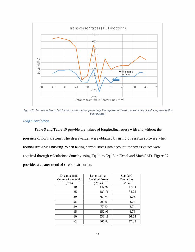
Figure 26. Transverse Stress Distribution across the Sample (orange line represents the triaxial state and blue line represents the biaxial state)
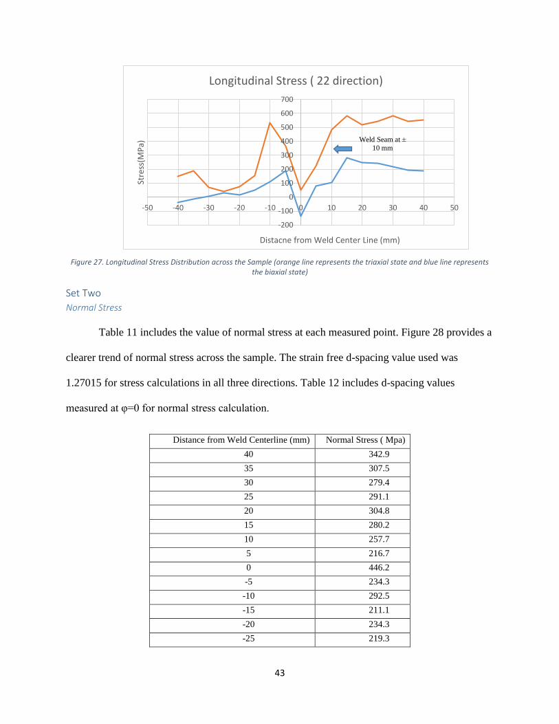
Longitudinal Stress
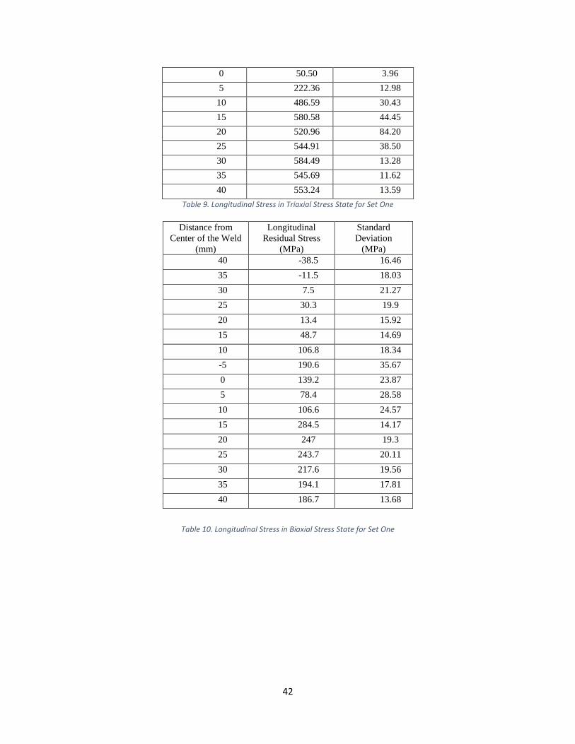
Table 9 and Table 10 provide the values of longitudinal stress with and without the
presence of normal stress. The stress values were obtained by using StressPlus software when
normal stress was missing. When taking normal stress into account, the stress values were
acquired through calculations done by using Eq.11 to Eq.15 in Excel and MathCAD. Figure 27
provides a clearer trend of stress distribution.
Distance from
Center of the Weld
(mm)
Longitudinal
Residual Stress
( MPa)
Standard
Deviation
(MPa)
40 147.07 17.34
35 189.71 34.25
30 67.74 5.08
25 38.45 4.97
20 77.40 8.74
15 152.96 3.76
10 531.11 16.64
-5 366.83 17.02
-200
-100
0
100
200
300
400
500
600
700
-50 -40 -30 -20 -10 0 10 20 30 40 50
Stre
ss (
MP
a)
Distance from Weld Center Line ( mm)
Transverse Stress (11 Direction)
Weld Seam at
±10mm
42
0 50.50 3.96
5 222.36 12.98
10 486.59 30.43
15 580.58 44.45
20 520.96 84.20
25 544.91 38.50
30 584.49 13.28
35 545.69 11.62
40 553.24 13.59
Table 9. Longitudinal Stress in Triaxial Stress State for Set One
Table 10. Longitudinal Stress in Biaxial Stress State for Set One
Distance from
Center of the Weld
(mm)
Longitudinal
Residual Stress
(MPa)
Standard
Deviation
(MPa)
40 -38.5 16.46
35 -11.5 18.03
30 7.5 21.27
25 30.3 19.9
20 13.4 15.92
15 48.7 14.69
10 106.8 18.34
-5 190.6 35.67
0 139.2 23.87
5 78.4 28.58
10 106.6 24.57
15 284.5 14.17
20 247 19.3
25 243.7 20.11
30 217.6 19.56
35 194.1 17.81
40 186.7 13.68
43
Figure 27. Longitudinal Stress Distribution across the Sample (orange line represents the triaxial state and blue line represents the biaxial state)
Set Two
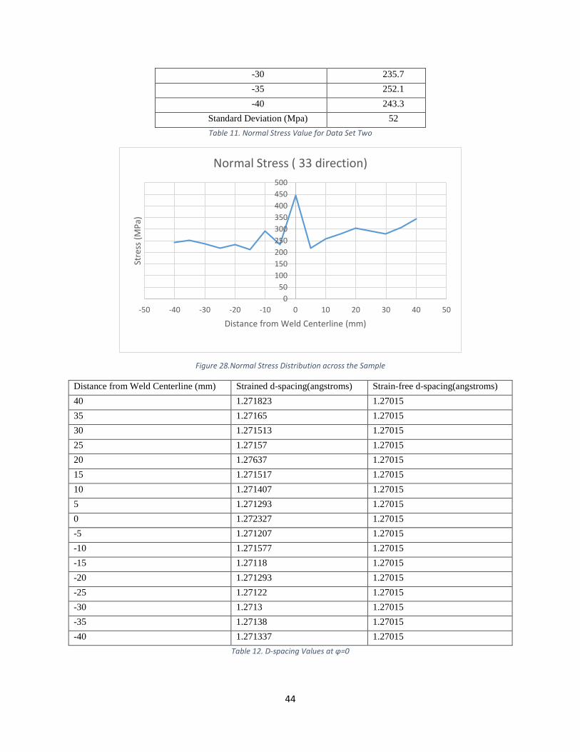
Normal Stress
Table 11 includes the value of normal stress at each measured point. Figure 28 provides a
clearer trend of normal stress across the sample. The strain free d-spacing value used was
1.27015 for stress calculations in all three directions. Table 12 includes d-spacing values
measured at φ=0 for normal stress calculation.
Distance from Weld Centerline (mm) Normal Stress ( Mpa)
40 342.9
35 307.5
30 279.4
25 291.1
20 304.8
15 280.2
10 257.7
5 216.7
0 446.2
-5 234.3
-10 292.5
-15 211.1
-20 234.3
-25 219.3
-200
-100
0
100
200
300
400
500
600
700
-50 -40 -30 -20 -10 0 10 20 30 40 50
Stre
ss(M
Pa)
Distacne from Weld Center Line (mm)
Longitudinal Stress ( 22 direction)
Weld Seam at ±
10 mm
44
-30 235.7
-35 252.1
-40 243.3
Standard Deviation (Mpa) 52
Table 11. Normal Stress Value for Data Set Two
Figure 28.Normal Stress Distribution across the Sample
Distance from Weld Centerline (mm) Strained d-spacing(angstroms) Strain-free d-spacing(angstroms)
40 1.271823 1.27015
35 1.27165 1.27015
30 1.271513 1.27015
25 1.27157 1.27015
20 1.27637 1.27015
15 1.271517 1.27015
10 1.271407 1.27015
5 1.271293 1.27015
0 1.272327 1.27015
-5 1.271207 1.27015
-10 1.271577 1.27015
-15 1.27118 1.27015
-20 1.271293 1.27015
-25 1.27122 1.27015
-30 1.2713 1.27015
-35 1.27138 1.27015
-40 1.271337 1.27015
Table 12. D-spacing Values at φ=0
0
50
100
150
200
250
300
350
400
450
500
-50 -40 -30 -20 -10 0 10 20 30 40 50
Stre
ss (
MP
a)
Distance from Weld Centerline (mm)
Normal Stress ( 33 direction)
45
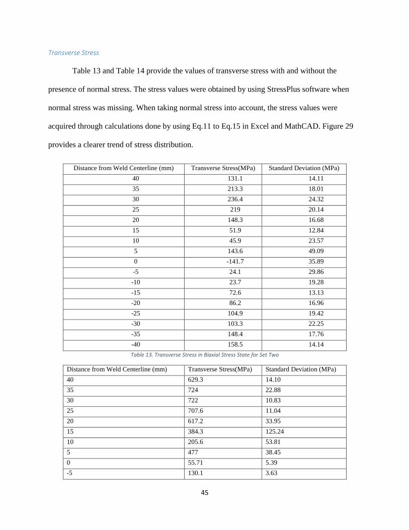
Transverse Stress
Table 13 and Table 14 provide the values of transverse stress with and without the
presence of normal stress. The stress values were obtained by using StressPlus software when
normal stress was missing. When taking normal stress into account, the stress values were
acquired through calculations done by using Eq.11 to Eq.15 in Excel and MathCAD. Figure 29
provides a clearer trend of stress distribution.
Distance from Weld Centerline (mm) Transverse Stress(MPa) Standard Deviation (MPa)
40 131.1 14.11
35 213.3 18.01
30 236.4 24.32
25 219 20.14
20 148.3 16.68
15 51.9 12.84
10 45.9 23.57
5 143.6 49.09
0 -141.7 35.89
-5 24.1 29.86
-10 23.7 19.28
-15 72.6 13.13
-20 86.2 16.96
-25 104.9 19.42
-30 103.3 22.25
-35 148.4 17.76
-40 158.5 14.14
Table 13. Transverse Stress in Biaxial Stress State for Set Two
Distance from Weld Centerline (mm) Transverse Stress(MPa) Standard Deviation (MPa)
40 629.3 14.10
35 724 22.88
30 722 10.83
25 707.6 11.04
20 617.2 33.95
15 384.3 125.24
10 205.6 53.81
5 477 38.45
0 55.71 5.39
-5 130.1 3.63
46
-10 240.4 82.58
-15 367.3 0.26
-20 364.5 16.22
-25 349.5 45.75
-30 365.9 61.84
-35 434.4 22.68
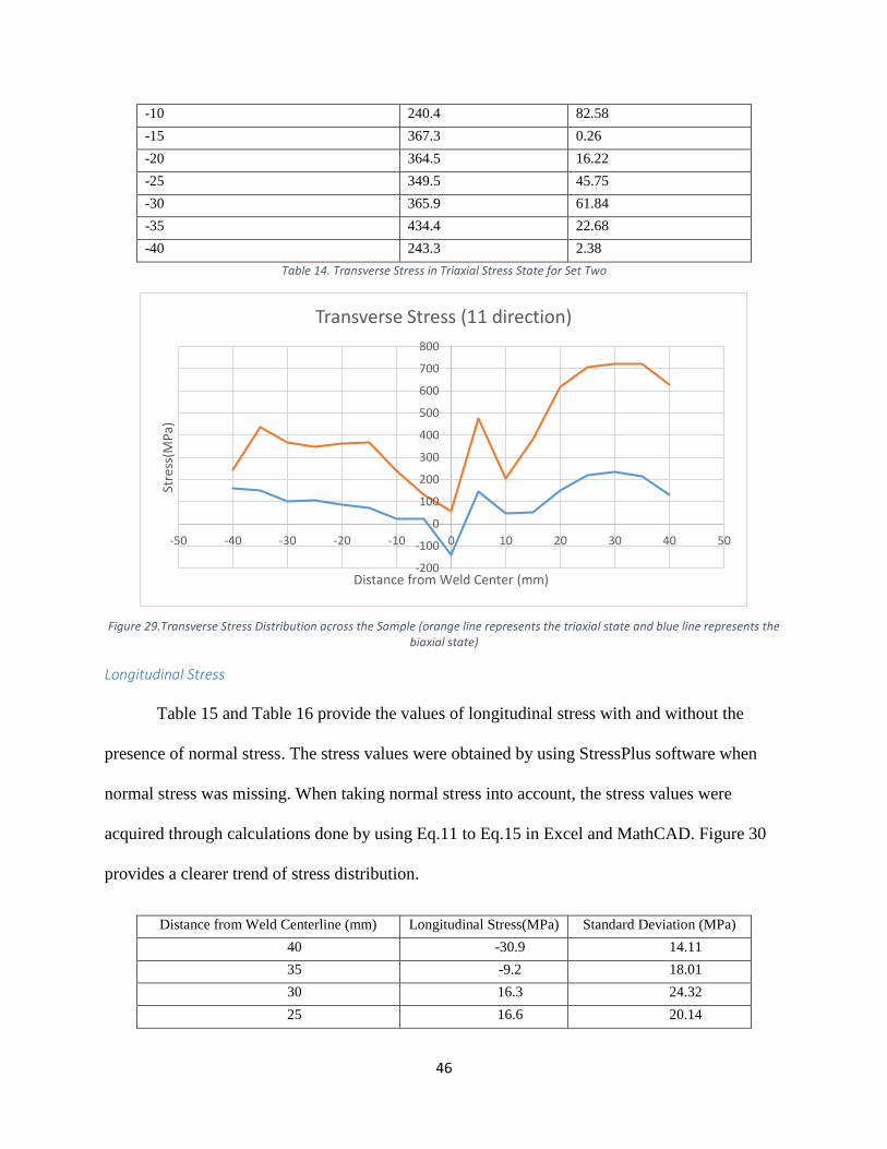
-40 243.3 2.38
Table 14. Transverse Stress in Triaxial Stress State for Set Two
Figure 29.Transverse Stress Distribution across the Sample (orange line represents the triaxial state and blue line represents the biaxial state)
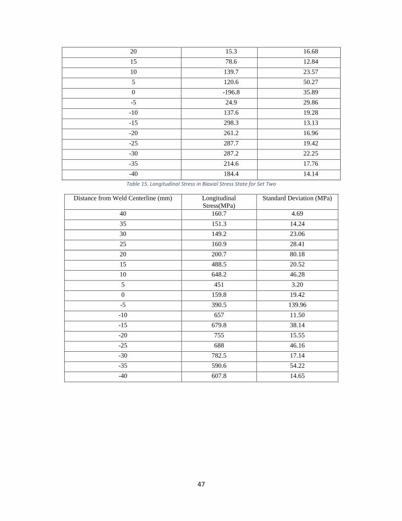
Longitudinal Stress
Table 15 and Table 16 provide the values of longitudinal stress with and without the
presence of normal stress. The stress values were obtained by using StressPlus software when
normal stress was missing. When taking normal stress into account, the stress values were
acquired through calculations done by using Eq.11 to Eq.15 in Excel and MathCAD. Figure 30
provides a clearer trend of stress distribution.
Distance from Weld Centerline (mm) Longitudinal Stress(MPa) Standard Deviation (MPa)
40 -30.9 14.11
35 -9.2 18.01
30 16.3 24.32
25 16.6 20.14
-200
-100
0
100
200
300
400
500
600
700
800
-50 -40 -30 -20 -10 0 10 20 30 40 50
Stre
ss(M
Pa)
Distance from Weld Center (mm)
Transverse Stress (11 direction)
47
20 15.3 16.68
15 78.6 12.84
10 139.7 23.57
5 120.6 50.27
0 -196.8 35.89
-5 24.9 29.86
-10 137.6 19.28
-15 298.3 13.13
-20 261.2 16.96
-25 287.7 19.42
-30 287.2 22.25
-35 214.6 17.76
-40 184.4 14.14
Table 15. Longitudinal Stress in Biaxial Stress State for Set Two
Distance from Weld Centerline (mm) Longitudinal
Stress(MPa)
Standard Deviation (MPa)
40 160.7 4.69
35 151.3 14.24
30 149.2 23.06
25 160.9 28.41
20 200.7 80.18
15 488.5 20.52
10 648.2 46.28
5 451 3.20
0 159.8 19.42
-5 390.5 139.96
-10 657 11.50
-15 679.8 38.14
-20 755 15.55
-25 688 46.16
-30 782.5 17.14
-35 590.6 54.22
-40 607.8 14.65
48
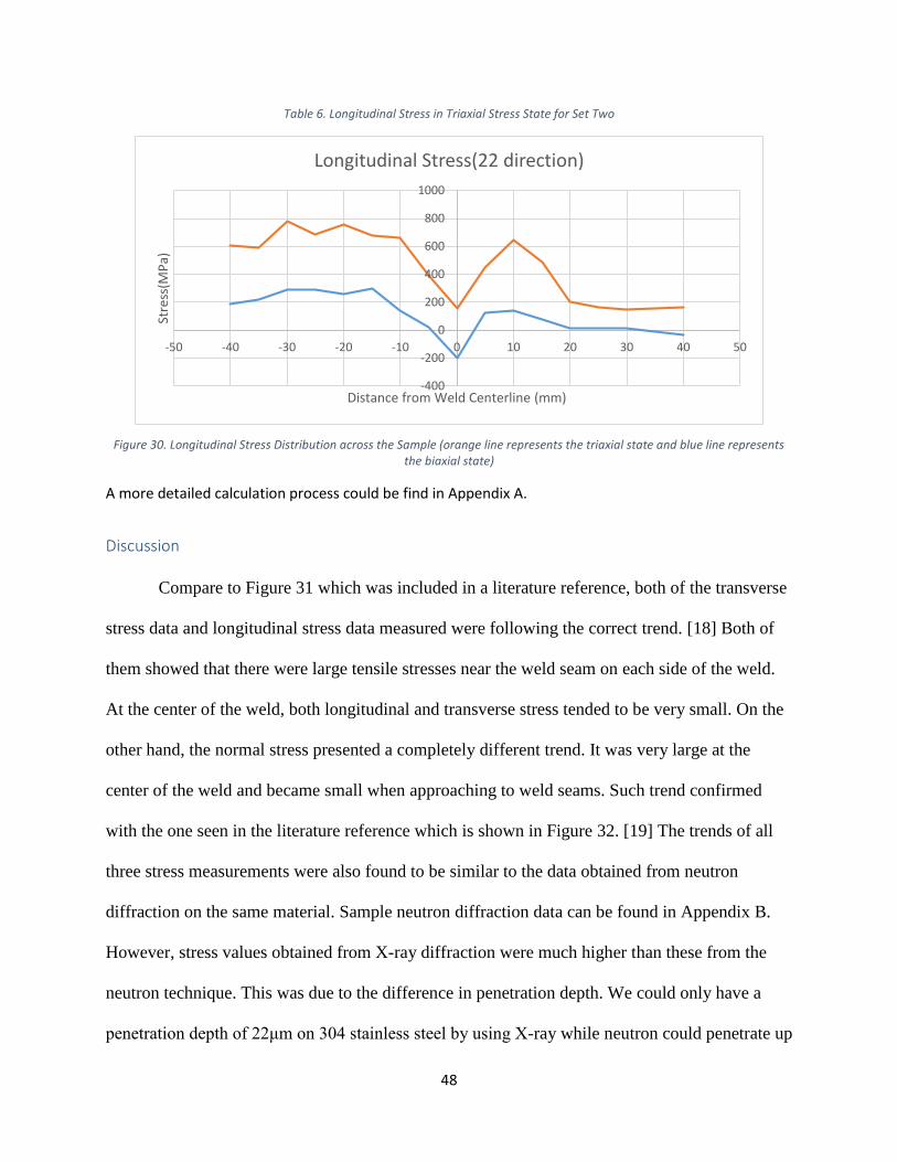
Table 6. Longitudinal Stress in Triaxial Stress State for Set Two
Figure 30. Longitudinal Stress Distribution across the Sample (orange line represents the triaxial state and blue line represents the biaxial state)
A more detailed calculation process could be find in Appendix A.
Discussion
Compare to Figure 31 which was included in a literature reference, both of the transverse
stress data and longitudinal stress data measured were following the correct trend. [18] Both of
them showed that there were large tensile stresses near the weld seam on each side of the weld.
At the center of the weld, both longitudinal and transverse stress tended to be very small. On the
other hand, the normal stress presented a completely different trend. It was very large at the
center of the weld and became small when approaching to weld seams. Such trend confirmed
with the one seen in the literature reference which is shown in Figure 32. [19] The trends of all
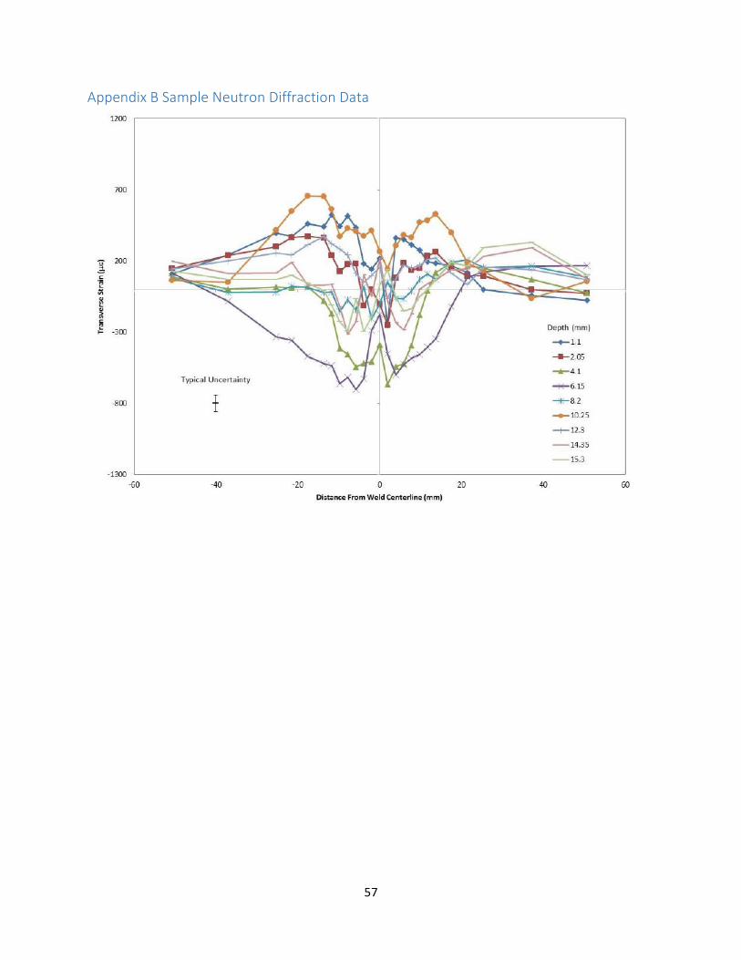
three stress measurements were also found to be similar to the data obtained from neutron
diffraction on the same material. Sample neutron diffraction data can be found in Appendix B.
However, stress values obtained from X-ray diffraction were much higher than these from the
neutron technique. This was due to the difference in penetration depth. We could only have a
penetration depth of 22μm on 304 stainless steel by using X-ray while neutron could penetrate up
-400
-200
0
200
400
600
800
1000
-50 -40 -30 -20 -10 0 10 20 30 40 50
Stre
ss(M
Pa)
Distance from Weld Centerline (mm)
Longitudinal Stress(22 direction)
49
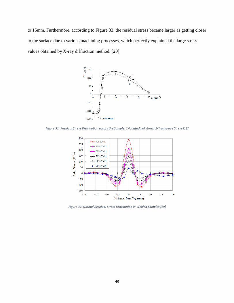
to 15mm. Furthermore, according to Figure 33, the residual stress became larger as getting closer
to the surface due to various machining processes, which perfectly explained the large stress
values obtained by X-ray diffraction method. [20]
Figure 31. Residual Stress Distribution across the Sample: 1-longtudinal stress; 2-Transverse Stress [18]
Figure 32. Normal Residual Stress Distribution in Welded Samples [19]
50
Figure 33. Surface Stress Distribution of As-machined Welded Sample [20]
When calculating transverse and longitudinal stresses, we looked into two cases: normal
stress was zero and normal stress was nonzero. The stress values without the presence of normal
stress were obtained through StressPlus software. Such software assumed the normal stress to be
zero since the penetration depth was really small. Therefore, the software adopted the equations
for calculating stress in a biaxial state automatically. However, according to the dψ vs. sin2 ψ
diagrams generated for each measurement point, there existed a split between measurements at
positive and negative φ angle. Such information suggested that the normal stress could not be
neglected. Since the software could not identify such situation, calculations were done by hand
by using Eq.11 to Eq. 15. The stress values obtained with and without the presence of normal
stress were compared in Figure 26, Figure 27, Figure 29, and Figure 30. From these figures, it
could be concluded that normal stress had a huge influence to both transverse and longitudinal
stress. It was important to have an accurate normal stress value so that the strain free d-spacing
must be experimentally measured carefully. Data set one and data set two only used a slightly
different d-spacing values but stress values showed more difference. Since d0 used for data set
51
two was taking from an annealed sample at its normalizing temperature, such value should be
used for better accuracy.
There were various sources of error that might need to be consider. The first one was the
misalignment of the instrument and the measuring samples. Detectors might misalign over usage
time without causing any notice to the users so that it could affect the results obtained. During
stress measurement, users were required to rotate the sample manually to different ϕ. Such
rotation might contain minor errors which could also influence the results. Secondly, the
sample’s surface might also cause errors in data. The samples being tested might not be flat
throughout their entire surface and since stress measurement by X-ray diffraction was sensitive
to sample’s height, errors might occur. Thirdly, the peak locations might not be identified
accurately by the software due to small background noise. Lastly, the strain-free d-spacing value
might not be the most accurate one due to cutting after annealing. Cutting might induce small
residual stress to the sample which could result in distorted lattice parameter. [15]
Conclusion
The 304 stainless steel welded plates were susceptible to stress corrosion cracking
through chlorine containing environment and residual stress due to welding. According to the
phase diagram and microstructure figure, our samples possessed typical characteristics of 304
stainless steel. The hardness tests furthered confirmed that our samples were annealed after
welding. From the stress measurements by using X-ray diffraction, we were able to see that at
the weld seam on each side of the weld, there existed large tensile stresses in both transverse and
longitudinal direction. At the center of the weld, stress values in both directions dropped sharply.
The normal stress shared a completely different trend. It tended to be the maximum at the center
52
of the weld and it became smaller while approaching the weld seam on each side. The stress
trends in all three directions were confirmed by literature references and stress data obtained
from neutron diffraction on the same material. However, the stress values measured by X-ray
diffraction were large compared to the ones acquired from neutron method. This was due to the
difference in penetration depth. X-ray diffraction could only had a penetration depth of 22µm
into the 304 stainless steel samples while neutron could have up to 15mm. The stress values near
the surface tended to become very large due to various machining processes. There could be
some sources of error such as instrument misalignment, rough sample surface, wrong peak
searching in software, and inaccurate strain-free d-spacing values.
53
Bibliography
[1] R. Ballinger, "Life Prediction of Spent Fuel Storage Canister Material," U.S.Department of Energy,
2014.
[2] "United States Nulcear Regulation Commission," 20th October 2014. [Online]. Available:
http://www.nrc.gov/waste/spent-fuel-storage/diagram-typical-dry-cask-system.html.
[3] "Nuclear Power Technology," 13th April 2014. [Online]. Available:
http://criepi.denken.or.jp/en/activities/project/nuclear.html.
[4] R. Parrott and H. Pitts, "Chloride Stress Corrosion Cracking in Austenitic Stainless Steel," Health and
Safety Executive, Derbyshire, 2011.
[5] G. Schajer and C. Ruud, "Overview of Residual Stresses and Their Measurement," in Practical
Residual Stress Measurement Methods, Vancouver, WILEY, 2013, pp. 1-29.
[6] P. Cole, C. Ikeagu, A. Thistlethwaite, S. Williams, T. Nagy, W. Suder, A. Steuwer and T. Pirling, "The
Welding Process Impact on Residual Stress and Distortion," Science and Technology of Welding
and Joining , pp. 717-725, 2009.
[7] "AK Steel," 3rd April 2014. [Online]. Available:
http://www.aksteel.com/pdf/markets_products/stainless/austenitic/304_304L_Data_Sheet.pdf.
[8] S. Chosh and V. Kain, "Microstrutual Changes in AISI 304L Stainless Steel due to Surface Machining:
Effect on its Susceptibility to Chloride Stress Corrosion Cracking," Journal of Nulcear Materials , pp.
62-67, 2010.
[9] M. Prime and A. DeWald, "The Contour Method," in Practical Residual Stress Measurement
Methods, Vancouver, WILEY, 2013, pp. 109-135.
[10] C. Murray and I. C. Noyan, "Applied and Residual Stress Determination Using X-ray Diffraction," in
Practical Residual Stress Measurement Methods, Vancouver, University of British Columbia , 2013,
pp. 139-161.
[11] T. Holden, "Neutron Diffraction," in Practical Residual Stress Measurement Methods , Vancouver,
WILEY, 2013, pp. 195-221.
[12] G. Schajer and P. Whitehead, "Hole Drilling and Ring Coring," in Practical Residual Stress
Measurement Methods , Vancouver, WILEY, 2013, pp. 29-61.
[13] M. Bateni, J. Szpunar, X. Wang and D. Li, "Wear and Corrosion Wear of Medium Carbon Steel and
304 Stainless Steel," WEAR, pp. 116-122, 2006.
[14] "ASTM Standards Info," 13th April 2015. [Online]. Available:
http://astm.nufu.eu/std/ASTM+E2860+-+12.
54
[15] B. D. Cullity, Elements Of X Ray Diffraction, New Jersey: Prentice Hall , 2001.
[16] D. Ye, Y. Xu, L. Xiao and H. Cha, "Effects of Low-cycle Fatigue on Static Mechanical Properties,
Microstructures, and Fracture Behavior of 304 Stainless Steel," Materials Science & Engineering ,
pp. 4092-4102, 2010.
[17] "Lucideon," 20th April 2014. [Online]. Available: http://www.ceram.com/testing-
analysis/techniques/x-ray-diffraction-xrd/rietveld-refinement/.
[18] J. Assis, V. Monin, J. Teodosio and T. Curova, "X-ray Analysis of Residual Stress Distribution in Weld
Region," Advances in X-ray Analysis, pp. 225-231, 2002.
[19] "Mitigation of Weld Induced Residual Stresses by Mechanical Stress Relieving," Pakistan Research
Repository, pp. 141-178.
[20] D. Thibault, P. Bocher and M. Thomas, "Residual Stress and Microstructure in Welds of 13%Cr–
4%Ni Martensitic Stainless Steel," Journal of Materials Processing Technology, pp. 2195-2202,
2009.
[21] "Wasteland: the 50-year battle to entomb our toxic nuclear remains," 13th April 2014. [Online].
Available: http://www.theverge.com/2012/6/14/3038814/yucca-mountain-wipp-wasteland-
battle-entomb-nuclear-waste.
55
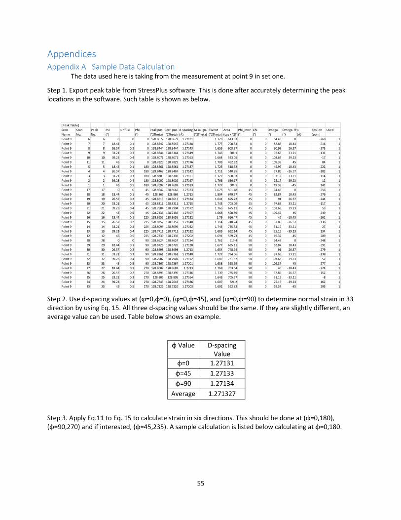
Appendices Appendix A Sample Data Calculation The data used here is taking from the measurement at point 9 in set one.
Step 1. Export peak table from StressPlus software. This is done after accurately determining the peak locations in the software. Such table is shown as below.
Step 2. Use d-spacing values at (ϕ=0,φ=0), (ϕ=0,φ=45), and (ϕ=0,φ=90) to determine normal strain in 33 direction by using Eq. 15. All three d-spacing values should be the same. If they are slightly different, an average value can be used. Table below shows an example.
φ Value D-spacing Value
φ=0 1.27131
φ=45 1.27133
φ=90 1.27134
Average 1.271327
Step 3. Apply Eq.11 to Eq. 15 to calculate strain in six directions. This should be done at (φ=0,180), (φ=90,270) and if interested, (φ=45,235). A sample calculation is listed below calculating at φ=0,180.
[Peak Table]
Scan Scan Peak Psi sin²Psi Phi Peak pos. Corr. pos. d-spacing Misalign. FWHM Area Phi_instr Chi Omega Omega-Thetaa Epsilon Used
Name No. No. (°) (°) (°2Theta) (°2Theta) (Å) (°2Theta) (°2Theta) (cps x °2Theta)(°) (°) (°) (°) (Å) (ppm)
Point 9 6 6 0 0 0 128.8672 128.8672 1.27131 1.723 613.63 0 0 64.43 0 -268 1
Point 9 7 7 18.44 0.1 0 128.8547 128.8547 1.27138 1.777 700.33 0 0 82.86 18.43 -216 1
Point 9 8 8 26.57 0.2 0 128.8444 128.8444 1.27143 1.655 603.37 0 0 90.99 26.57 -173 1
Point 9 9 9 33.21 0.3 0 128.8344 128.8344 1.27149 1.743 601.1 0 0 97.63 33.21 -131 1
Point 9 10 10 39.23 0.4 0 128.8071 128.8071 1.27163 1.664 523.05 0 0 103.64 39.23 -17 1
Point 9 11 11 45 0.5 0 128.7829 128.7829 1.27176 1.703 492.82 0 0 109.39 45 84 1
Point 9 5 5 18.44 0.1 180 128.8561 128.8561 1.27137 1.725 518.52 0 0 45.99 -18.43 -222 1
Point 9 4 4 26.57 0.2 180 128.8467 128.8467 1.27142 1.711 540.95 0 0 37.86 -26.57 -182 1
Point 9 3 3 33.21 0.3 180 128.8303 128.8303 1.27151 1.722 598.03 0 0 31.2 -33.21 -114 1
Point 9 2 2 39.23 0.4 180 128.8002 128.8002 1.27167 1.766 636.17 0 0 25.17 -39.23 12 1
Point 9 1 1 45 0.5 180 128.7692 128.7692 1.27183 1.727 604.1 0 0 19.38 -45 141 1
Point 9 17 17 0 0 45 128.8642 128.8642 1.27133 1.673 591.48 45 0 64.43 0 -256 1
Point 9 18 18 18.44 0.1 45 128.869 128.869 1.2713 1.804 649.37 45 0 82.87 18.43 -276 1
Point 9 19 19 26.57 0.2 45 128.8613 128.8613 1.27134 1.641 695.22 45 0 91 26.57 -244 1
Point 9 20 20 33.21 0.3 45 128.8311 128.8311 1.2715 1.743 703.09 45 0 97.63 33.21 -117 1
Point 9 21 21 39.23 0.4 45 128.7904 128.7904 1.27172 1.766 675.11 45 0 103.63 39.23 53 1
Point 9 22 22 45 0.5 45 128.7436 128.7436 1.27197 1.668 590.89 45 0 109.37 45 249 1
Point 9 16 16 18.44 0.1 225 128.8655 128.8655 1.27132 1.79 656.47 45 0 46 -18.43 -261 1
Point 9 15 15 26.57 0.2 225 128.8357 128.8357 1.27148 1.714 748.74 45 0 37.85 -26.57 -136 1
Point 9 14 14 33.21 0.3 225 128.8095 128.8095 1.27162 1.745 735.33 45 0 31.19 -33.21 -27 1
Point 9 13 13 39.23 0.4 225 128.7711 128.7711 1.27182 1.685 662.14 45 0 25.15 -39.23 134 1
Point 9 12 12 45 0.5 225 128.7339 128.7339 1.27202 1.691 569.73 45 0 19.37 -45 289 1
Point 9 28 28 0 0 90 128.8624 128.8624 1.27134 1.761 619.4 90 0 64.43 0 -248 1
Point 9 29 29 18.44 0.1 90 128.8726 128.8726 1.27128 1.677 685.11 90 0 82.87 18.43 -291 1
Point 9 30 30 26.57 0.2 90 128.8698 128.8698 1.2713 1.654 748.94 90 0 91 26.57 -279 1
Point 9 31 31 33.21 0.3 90 128.8361 128.8361 1.27148 1.727 794.06 90 0 97.63 33.21 -138 1
Point 9 32 32 39.23 0.4 90 128.7907 128.7907 1.27172 1.682 731.67 90 0 103.63 39.23 52 1
Point 9 33 33 45 0.5 90 128.7367 128.7367 1.27201 1.658 598.59 90 0 109.37 45 277 1
Point 9 27 27 18.44 0.1 270 128.8687 128.8687 1.2713 1.768 763.54 90 0 46 -18.43 -274 1
Point 9 26 26 26.57 0.2 270 128.8395 128.8395 1.27146 1.739 785.19 90 0 37.85 -26.57 -152 1
Point 9 25 25 33.21 0.3 270 128.805 128.805 1.27164 1.643 705.27 90 0 31.19 -33.21 -8 1
Point 9 24 24 39.23 0.4 270 128.7643 128.7643 1.27186 1.607 621.2 90 0 25.15 -39.23 162 1
Point 9 23 23 45 0.5 270 128.7326 128.7326 1.27203 1.692 552.82 90 0 19.37 -45 295 1
56
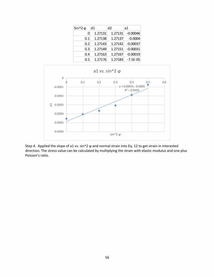
Step 4. Applied the slope of a1 vs. sin^2 ϕ and normal strain into Eq. 12 to get strain in interested direction. The stress value can be calculated by multiplying the strain with elastic modulus and one plus Poisson’s ratio.
Sin^2 ϕ d1 d2 a1
0 1.27131 1.27131 -0.00046
0.1 1.27138 1.27137 -0.0004
0.2 1.27143 1.27142 -0.00037
0.3 1.27149 1.27151 -0.00031
0.4 1.27163 1.27167 -0.00019
0.5 1.27176 1.27183 -7.5E-05
y = 0.0007x - 0.0005R² = 0.9493
-0.0006
-0.0005
-0.0004
-0.0003
-0.0002
-0.0001
0
0 0.1 0.2 0.3 0.4 0.5 0.6
a1
sin^2 ϕ
a1 vs. sin^2 ϕ
57
Appendix B Sample Neutron Diffraction Data
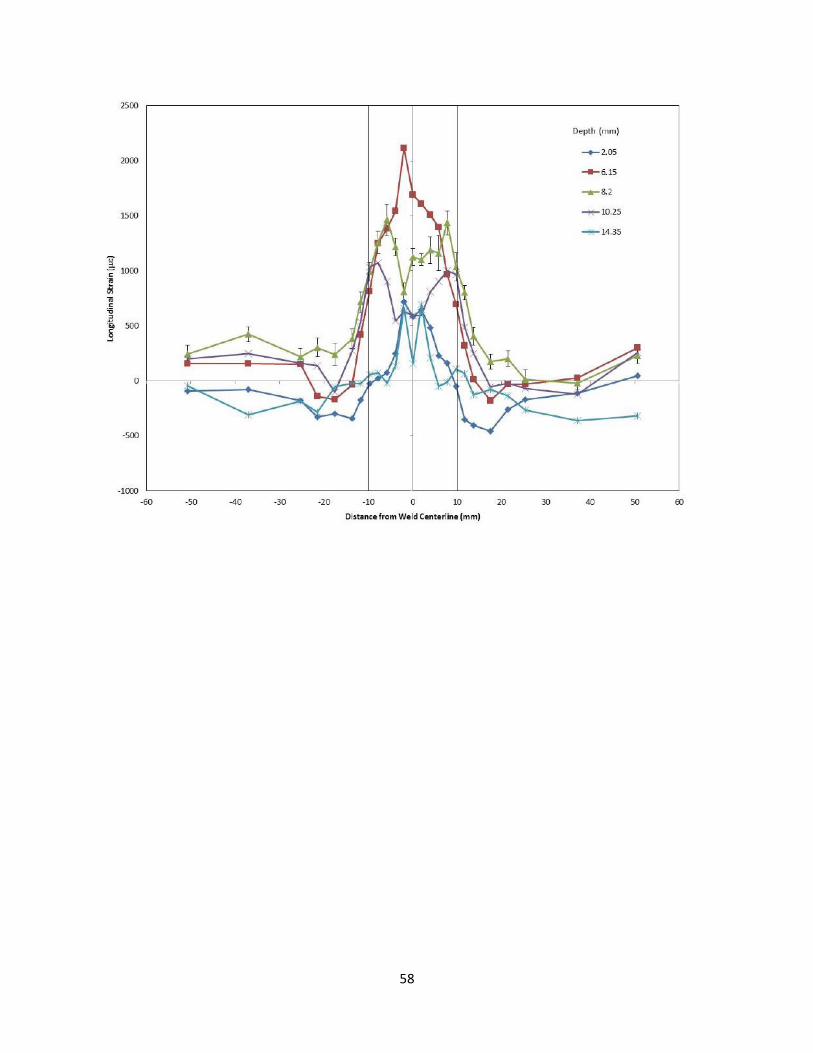
58
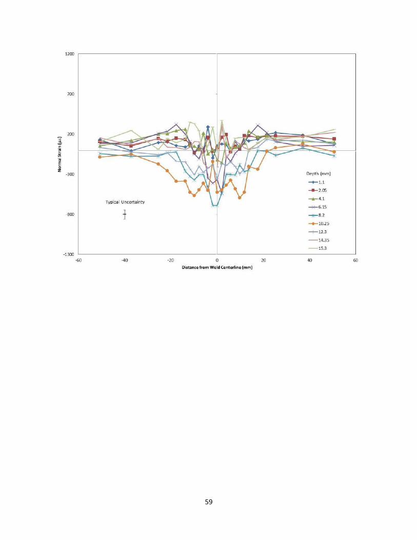
59