Embed Size (px)
Citation preview

Residual monomer reduction in polymer latex products byextraction with supercritical carbon dioxideCitation for published version (APA):Aerts, M. (2012). Residual monomer reduction in polymer latex products by extraction with supercritical carbondioxide. Eindhoven: Technische Universiteit Eindhoven. https://doi.org/10.6100/IR723144
DOI:10.6100/IR723144
Document status and date:Published: 01/01/2012
Document Version:Publisher’s PDF, also known as Version of Record (includes final page, issue and volume numbers)
Please check the document version of this publication:
• A submitted manuscript is the version of the article upon submission and before peer-review. There can beimportant differences between the submitted version and the official published version of record. Peopleinterested in the research are advised to contact the author for the final version of the publication, or visit theDOI to the publisher's website.• The final author version and the galley proof are versions of the publication after peer review.• The final published version features the final layout of the paper including the volume, issue and pagenumbers.Link to publication
General rightsCopyright and moral rights for the publications made accessible in the public portal are retained by the authors and/or other copyright ownersand it is a condition of accessing publications that users recognise and abide by the legal requirements associated with these rights.
• Users may download and print one copy of any publication from the public portal for the purpose of private study or research. • You may not further distribute the material or use it for any profit-making activity or commercial gain • You may freely distribute the URL identifying the publication in the public portal.
If the publication is distributed under the terms of Article 25fa of the Dutch Copyright Act, indicated by the “Taverne” license above, pleasefollow below link for the End User Agreement:www.tue.nl/taverne
Take down policyIf you believe that this document breaches copyright please contact us at:[email protected] details and we will investigate your claim.
Download date: 30. Mar. 2020

Residual monomer reduction in polymer latex products by
extraction with supercritical carbon dioxide
PROEFSCHRIFT ter verkrijging van de graad van doctor aan de Technische Universiteit Eindhoven, op gezag van de rector magnificus, prof.dr.ir. C.J. van Duijn, voor een commissie aangewezen door het College voor Promoties in het openbaar te verdedigen op dinsdag 7 februari 2012 om 16.00 uur door Marijke Aerts geboren te Hasselt, België

Dit proefschrift is goedgekeurd door de promotoren: prof.dr.ir. J.T.F. Keurentjes en prof.dr. J. Meuldijk A catalogue record is available from the Eindhoven University of Technology Library ISBN: 978-90-386-3073-1 © 2012, Marijke Aerts This research was financially supported by the Foundation of Emulsion Polymerization (SEP). Cover design: Nina Middelkamp and Marijke Aerts Printed at the Universiteitsdrukkerij, Eindhoven University of Technology

Niet alles draait om carrière en geld
Maar ook om liefde en vriendschap die je kunt geven,
Pas dan ben je ook geslaagd als mens voor de rest van je leven.


i
Table of Contents
Table of contents i
Summary iii
Samenvatting v
Chapter 1 Introduction: Residual monomer reduction in polymer emulsion polymerization products: Limitations and challenges 1
Chapter 2 Partitioning of residual monomer between polymer and CO2
– A theoretical approach 9 Chapter 3 Experimental determination of the partition coefficient of
monomers over polymer and supercritical carbon dioxide 27
Chapter 4 Mass transport phenomena in the supercritical carbon dioxide
extraction of residual monomer from latex products 61 Chapter 5 Process design for the residual monomer reduction in latex
with supercritical carbon dioxide 83 Chapter 6 High pressure carbon dioxide in the extraction of residual
monomer from latex products: additional results and outlook 137 Notation 147 Dankwoord 155 Curriculum Vitae 157


iii
Summary
Residual monomer reduction in polymer (latex) products by extraction with
supercritical carbon dioxide
The increased awareness for environmental issues as well as for public health, demands
“greener” processes as well as products. In the polymer industry, one of the major concerns
relate to residual monomer in polymer (latex) products. Low molecular species are toxic.
When monomer units diffuse out of their polymeric matrix, they contaminate the surrounding
area. Decreasing the residual monomer level in polymer (latex) products is especially of
great importance in food packaging, toys for children, etc. Conventional techniques to reduce
residual monomer in polymer (latex) products are energy intensive, time consuming and not
able to fulfill the increasingly stringent requirements for further reduction of residual monomer
in polymer products, i.e. < 100 parts per million (ppm).
In this thesis the reduction of residual monomer in polymer (latex) products by extraction with
supercritical carbon dioxide (scCO2) is explored. The Peng-Robinson equation of state has
been used to describe the binary phase diagram of CO2 and styrene as well as of CO2 and
methyl methacrylate. The ternary phase diagram of CO2-styrene-polystyrene as well as of
CO2-methyl methacrylate-polymethyl methacrylate has been estimated with the Perturbed
Chain - Statistical Associated Fluid Theory. The partition coefficient of the distribution of
monomer between CO2 and CO2 swollen polymer has been calculated.
In a high pressure autoclave the partition coefficient of the distribution of monomer between
CO2 and CO2 swollen polymer has been determined experimentally at a range of
temperatures and pressures. The experimental results demonstrate the partition coefficient is
approximately independent of pressure and temperature. For the partitioning of styrene
between CO2 and CO2 swollen polystyrene a value of 2 [kg PS/kg CO2] has been found,
while for the partitioning of methyl methacrylate between CO2 and CO2 swollen polymethyl
methacrylate a value of 0.3 [kg PMMA/kg CO2] has been determined.
Mass transport of monomer from the polymer phase to the CO2 phase is governed by the
shuttle effect. The monomer is hereby directly transferred from the polymer particles to the

Summary
iv
CO2 phase due to Brownian motion of the particles to and from the CO2/H2O interface. The
main resistance against mass transfer has been demonstrated to be located in the polymer
particles.
The countercurrent extraction process to reduce residual monomer in polymer (latex)
products from 104 ppm to 1 ppm in a column has been designed. Latex has been chosen as
the continuous phase in which 1 mm CO2 bubbles are dispersed with a hold up of 20 %. The
column is operated at 100 bar and 35 °C. A column volume of 4.75 m3 applies for a
throughput of 6000 kg PS latex (45% solids)/hr. The extraction process reducing the residual
monomer costs 22 €/ton latex for a production capacity of 50 kt PS latex (45% solids)/yr.
Continuous steam stripping only costs 12 €/ton latex to reduce the residual monomer level
from 104 to 100 ppm, whereas the purification costs of the CO2-based extraction process are
similar for a reduction to 100, 10 or 1 ppm. Reduction to lower levels of residual monomer,
lower than 100 ppm, by means of steam stripping is hardly possible, mainly due to
thermodynamic (and to some extent transport) limitations. The results of calculations for a
residual monomer reduction from 104 to 10 ppm with 100 °C steam point to a tremendous
increase of the utility costs. The costs of a continuous steam stripping process are then more
than 75 €/ton latex. The lowest residual monomer concentration in latex of 1 ppm can
certainly only be achieved by extraction with (sc)CO2.

v
Samenvatting
Verminderen van het restmonomeer gehalte in polymeren door middel van
extractie met superkritisch kooldioxide
“Groene” processen en producten worden steeds belangrijker in het dagelijkse leven door de
groeiende bezorgdheid om ons milieu, onze gezondheid en de beschikbaarheid van
(fossiele) grondstoffen. Eén van de grootste aandachtspunten bij de productie van polymere
materialen is het restmonomeer gehalte. Vooral in onder andere verpakkingsmateriaal voor
voeding en in speelgoed is het verminderen van restmonomeer van groot belang. De
technieken die nu gebruikt worden om restmonomeer in polymeer producten te verlagen zijn
tijdrovend, kosten veel energie en kunnen het restmonomeer gehalte niet tot het gewenste
niveau doen dalen , dat wil zeggen tot niveaus duidelijk lager dan 100 ppm.
In het in dit proefschrift beschreven werk is de extractie van restmonomeer uit polymeren
door middel van superkritisch CO2 (scCO2) bestudeerd. Het binaire fasengedrag van zowel
CO2 en styreen als van CO2 en methyl methacrylaat werd beschreven met de Peng-
Robinson toestandsvergelijking. Het ternaire fasendiagram van CO2-styreen-polystyreen en
van CO2-methyl methacrylaat-polymethyl methacrylaat werd in kaart gebracht met de
Perturbed Chain - Statistical Associated Fluid Theory (PC SAFT). De verdelingscoefficient
van monomeer over de CO2-fase en het polymeer gezwollen met CO2 is berekend met het
PC SAFT model.
De experimentele bepaling van de verdelingscoefficient van monomeer over de CO2 fase en
het polymeer gezwollen met CO2 werd uitgevoerd in een hoge druk cel bij verschillende
drukken en temperaturen. De experimentele resultaten laten zien dat de verdelingscoefficient
nagenoeg onafhankelijk is van druk en temperatuur. De gemeten waarden van de
verdelingscoëfficiënt wijken aanzienlijk af van de met PC SAFT berekende waarden. De
reden voor deze verschillen tussen de berekende en gemeten waarden is waarschijnlijk het
uitgangspunt bij de berekeningen. Bij de berekeningen is uitgegaan van een ideaal polymeer
zonder verknopingen (entanglements). Voor de metingen zijn niet-behandelde
reactorproducten gebruikt.

Samenvatting
vi
Het zogenaamde ‘shuttle effect’ domineert monomeer transport van de polymeer fase naar
de CO2 fase. De polymeerdeeltjes bewegen naar en van het CO2/H2O grensvlak ten gevolge
van de Brownse beweging. Hierdoor ontstaat er een direct contact tussen het
polymeerdeeltje en CO2, waardoor monomeer direct wordt overgedragen naar het CO2. De
grootste weerstand tegen het monomeertransport ligt in de polymeerdeeltjes.
Het tegenstroom extractie proces om het restmonomeer gehalte in polymeer te verlagen van
104 naar 1 ppm is ontworpen als een kolomproces. Latex is hierin de continue fase waarin 1
mm CO2 druppels worden gedispergeerd met een volumefractie van 0,2. De extractiekolom
is ontworpen voor een druk van 100 bar en een temperatuur van 35 °C. Voor het verwerken
van 6000 kg PS latex (45% droge stof)/uur, is een kolomvolume van 4.75 m³ berekend. De
kosten van de extractie van restmonomeer zijn geschat op 22 €/ton latex voor een productie
capaciteit van 50103 ton PS latex (45% droge stof)/jaar. Het verminderen van
restmonomeer van 104 tot 100 ppm met stoomstrippen als continu proces kost slechts 12
€/ton latex. De kosten voor de extractie met CO2 van 104 ppm restmonomeer naar 100, 10 of
1 ppm blijven echter ongeveer gelijk. Mogelijkheden om het restmonomeergehalte met
stoomstrippen verder te verlagen dan 100 ppm zijn zeer beperkt, omdat het proces zowel
thermodynamisch als wat betreft monomeertransport in de polymeerdeeltjes is gelimiteerd.
Een berekening voor het verlagen van restmonomeer van 104 naar 10 ppm met stoom
strippen toont een enorme stijging van de proceskosten, voornamelijk door de grote
hoeveelheid stoom die verbruikt wordt. Het continue stoom strip proces kost dan maar liefst
75 €/ton latex. Een restmonomeer niveau van 1 ppm kan enkel worden bereikt door middel
van extractie met scCO2.


1
Chapter 1
Introduction: Residual monomer reduction in polymer
emulsion polymerization products: Limitations and
challenges
Introduction
Emulsion polymerization is frequently used in industry to produce e.g. adhesives, latex
paints, coatings and rubbers (Gilbert, 1995). Emulsion polymerization is a free radical
polymerization in a heterogeneous reaction system, yielding a colloidally stable
dispersion of submicron polymer particles in an aqueous medium. The process is
governed by a complex mechanism, see e.g. Gilbert (1995) and van Herk (2005). In
many cases three time-separated stages can be distinguished in a batch process, i.e.
particle nucleation, particle growth in the presence of monomer droplets and completion
of the polymerization when the monomer droplets have been consumed. A simple
description of the mechanism of emulsion polymerization has first been given by Harkins
(1947) and later worked out by Smith and Ewart (1948). Many research groups have
studied the emulsion polymerization process, see e.g. Hansen and Ugelstad (1982),
Gilbert (1995), van Herk (2005), De la Cal et al. (2005) and De Cal et al. (2007).
However, complete insight into the whole process has not been reached up to now. In
general, emulsion polymerization yields a high molecular weight polymer product.
Typical values of the degree of polymerization are mostly considerable larger than 103.
Molecular mass can e.g. be reduced by chain transfer agents. In the last stage of the
process the rate of polymerization will decrease due to the decreasing monomer
concentration inside the particles. Due to diffusion limitations in the particle phase the
polymerization reaction will not proceed to completion. As a consequence, the polymer
Chapter 1
2
latex product contains a significant amount of residual monomer inside the polymer
particles, generally in the range of a thousand parts per million (ppm). Reduction of the
residual monomer level in polymer latex products is essential for safe and non-toxic use.
Moreover, increasingly stringent requirements demand for further reduction of residual
monomer in polymer products. Various conventional techniques to reduce the residual
monomer level in polymer latex products are energy intensive (e.g. steam stripping,
Englund, 1981), time consuming (e.g. temperature increase) or even might change the
product properties (e.g. addition of initiator). Most important, conventional techniques are
not able to fulfill the stringent requirements as the result of thermodynamic and transport
limitations.
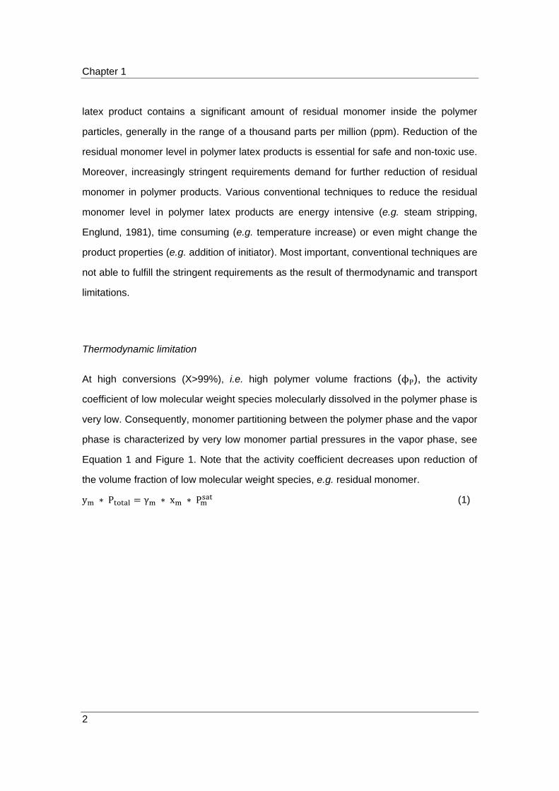
Thermodynamic limitation
At high conversions (X>99%), i.e. high polymer volume fractions (ϕP), the activity
coefficient of low molecular weight species molecularly dissolved in the polymer phase is
very low. Consequently, monomer partitioning between the polymer phase and the vapor
phase is characterized by very low monomer partial pressures in the vapor phase, see
Equation 1 and Figure 1. Note that the activity coefficient decreases upon reduction of
the volume fraction of low molecular weight species, e.g. residual monomer.
y ∗ P γ ∗ x ∗ P (1)
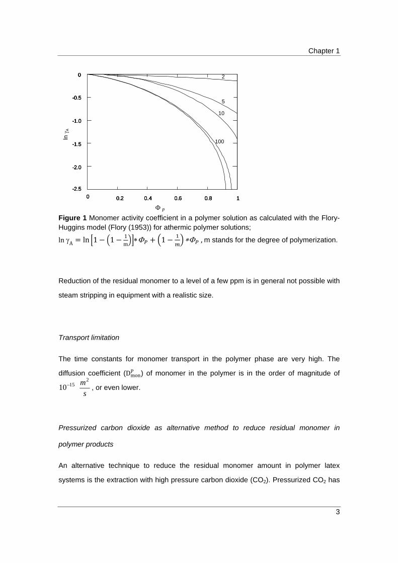
Chapter 1
3
Figure 1 Monomer activity coefficient in a polymer solution as calculated with the Flory-Huggins model (Flory (1953)) for athermic polymer solutions;
lnA ln 1 1 1m
1 ,m stands for the degree of polymerization.
Reduction of the residual monomer to a level of a few ppm is in general not possible with
steam stripping in equipment with a realistic size.
Transport limitation
The time constants for monomer transport in the polymer phase are very high. The
diffusion coefficient (DmonP ) of monomer in the polymer is in the order of magnitude of
s
m21510 , or even lower.
Pressurized carbon dioxide as alternative method to reduce residual monomer in
polymer products
An alternative technique to reduce the residual monomer amount in polymer latex
systems is the extraction with high pressure carbon dioxide (CO2). Pressurized CO2 has
P
0
-0.5
-1.0
-1.5
-2.0
-2.5
0 0.2 0.4 0.6 0.8 1
2
5
10
100
0
-0.5
-1.0
-1.5
-2.0
-2.5
0 0.2 0.4 0.6 0.8 1
0
-0.5
-1.0
-1.5
-2.0
-2.5
0 0.2 0.4 0.6 0.8 1
2
5
10
100
ln
A

Chapter 1
4
several advantages to be used as extraction medium. At conditions above the critical
temperature (304 K) and the critical pressure (73 bar) of CO2 (Poling et al., 2001), the
physical properties lie between those of a liquid and a gas, combining favorable qualities
of the liquid phase as well as the gas phase, see Table 1. For example, at high
pressures a SCF has solubility and density properties close to those of a liquid, but with
considerable larger diffusion coefficients and lower viscosity.
Table 1 Typical properties of gases, supercritical fluids (SCF) and liquids property gas SCF liquid
density (kg/m³) 1 100-800 1000
viscosity (mPa.s) 0.01 0.05-0.1 0.5-1
diffusivity (m²/s) 10-5 10-7 10-9
High pressure extraction with near supercritical or supercritical fluids (SCF) has been in
use for several decades on an industrial scale (Kilzer et al., 2011, Morgan, 2000, Araújo,
2002), e.g. for the decaffeination of coffee. Relatively small changes in the CO2 pressure
as well as in temperature result in large density changes favoring the extraction process.
The most important advantage of using high pressure CO2 is that CO2 increases the
fugacity of the monomer in the polymer phase (i.e. decreasing ϕP by swelling the
polymer with CO2), thereby increasing the monomer molar fraction in the gas or SCF
phase, see Equation 1.
Note that as a result of swelling the polymer is softened and plasticized. Monomer
transport rates (in terms of DmonP ) in the polymer phase swollen with CO2 increase from
values 10 to about 10 or even higher (Alsoy and Duda, 1998), leading to
improved monomer transport rates compared to e.g. steam stripping. Note that for highly
amorphous or rubbery polymers, a maximum can be reached in the mass transfer rate
with increasing pressure (Vandenburg, 2000). With increasing pressure, i.e. more CO2
uptake in the polymer matrix, the softening point of the polymer, i.e. the glass transition
temperature Tg, decreases. If Tg falls below the operation temperature in the extraction
process, the polymer particles will become sticky and the extraction process is
Chapter 1
5
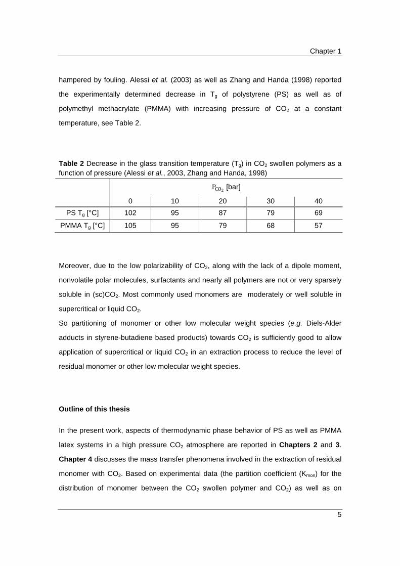
hampered by fouling. Alessi et al. (2003) as well as Zhang and Handa (1998) reported
the experimentally determined decrease in Tg of polystyrene (PS) as well as of
polymethyl methacrylate (PMMA) with increasing pressure of CO2 at a constant
temperature, see Table 2.
Table 2 Decrease in the glass transition temperature (Tg) in CO2 swollen polymers as a function of pressure (Alessi et al., 2003, Zhang and Handa, 1998) PCO2 [bar]
0 10 20 30 40
PS Tg [°C] 102 95 87 79 69
PMMA Tg [°C] 105 95 79 68 57
Moreover, due to the low polarizability of CO2, along with the lack of a dipole moment,
nonvolatile polar molecules, surfactants and nearly all polymers are not or very sparsely
soluble in (sc)CO2. Most commonly used monomers are moderately or well soluble in
supercritical or liquid CO2.
So partitioning of monomer or other low molecular weight species (e.g. Diels-Alder
adducts in styrene-butadiene based products) towards CO2 is sufficiently good to allow
application of supercritical or liquid CO2 in an extraction process to reduce the level of
residual monomer or other low molecular weight species.
Outline of this thesis
In the present work, aspects of thermodynamic phase behavior of PS as well as PMMA
latex systems in a high pressure CO2 atmosphere are reported in Chapters 2 and 3.
Chapter 4 discusses the mass transfer phenomena involved in the extraction of residual
monomer with CO2. Based on experimental data (the partition coefficient (Kmon) for the
distribution of monomer between the CO2 swollen polymer and CO2) as well as on

Chapter 1
6
theoretically predicted parameters (dispersed phase hold up, droplet size) the design of
an extraction process is described in Chapter 5. In Chapter 5 also an economic
evaluation of the CO2 based extraction process is given. The results of this evaluation
are compared with the results of a cost estimation of a steam stripping process. In
Chapter 6 additional comments as well as the challenges and opportunities in field of
extraction of residual monomer from polymer (latex) products with scCO2 are presented.
Chapter 1
7
References P. Alessi, A. Cortesi, I. Kikic, F. Vecchione, “Plasticization of polymers with supercritical carbon dioxide: Experimental determination of glass-transition temperatures”, J. Appl. Polym. Sci., 2003, 88, 2189-2193 S. Alsoy, J. L. Duda, “Supercritical devolatilization of polymers”, AIChE, 1998, 44, 3, 582-590 P. H. H. Araújo, C. Sayer, J. G. R. Poço, R. Guidici, “Techniques for reducing residual monomer content in polymers: A review”, Polym. Eng. Sci., 2002, 42, 7 J. C. De La Cal, J. R. Leiza, J. M. Asua, A. Buttè, G. Storti, M. Morbidelli, “Emulsion polymerization”, in “Handbook of polymer reaction engineering”, J. T. F. Keurentjes, T. Meyer, Eds., 2005, Wiley-VCH, Weinheim J. C. De La Cal, Chapter 6 in “Polymer reaction engineering”, J. M. Asua, Ed., 2007, Blackwell, Oxford S. M. Englund, “Monomer removal from latex”, Chem. Eng. Progr., 1981, 55-59; and references therein R. G. Gilbert, “Emulsion polymerization, A mechanistic approach”, Academic Press, 1995 Hansen, Ugelstad, Chapter 6 in “Emulsion polymerization, I. Piirma, Ed., Academic Press, 1982, London A. M. van Herk, “Chemistry and technology of Emulsion polymerization”, Ed., 2005, Blackwell, Oxford A. Kilzer, S. Kareth, E. Weidner, “Neue Entwicklungen bei Reinigungs- und Trennprozessen mit über- und nahkritischen Fluiden”, Chemie Ingenieur Technik, 2011, 83, 9, 1405–1418 E. D. Morgan, “III/Natural products/Supercritical fluid extraction”, Academic Press, 2000 Z. Zhang, Y. P. Handa, “An in situ study of plasticization of polymers by high-pressure gases”, J. Polym. Sci., Part B: Polym. Phys., 1998, 36, 977-982 H. J. Vandenburg, “III/Polymers/Supercritical fluid extraction”, Academic Press, 2000


9
Chapter 2
Partitioning of residual monomer between polymer and
CO2
– A theoretical approach
Abstract
The efficiency of high pressure carbon dioxide to reduce residual monomer level in polymer
products strongly depends on the monomer partitioning over the various phases involved in
the separation process.
Phase behavior of the styrene – carbon dioxide as well as of the methyl methacrylate –
carbon dioxide binary systems has been modeled with the Peng-Robinson equation of state.
Monomer partitioning between the polystyrene or polymethyl methacrylate phase and the
CO2 phase has been estimated with the Perturbed Chain – Statistical Associated Fluid
Theory (PC-SAFT).
Introduction
Extraction with supercritical or high pressure carbon dioxide ((sc)CO2) is an interesting
alternative to e.g. steam stripping to reduce the residual monomer level in polymer (latex)
products. Knowledge of the phase behavior of the system monomer/polymer (latex)/(sc)CO2
as a function of various operating conditions is a necessary prerequisite for process design.

Chapter 2
10
Vapor-liquid phase equilibria at high pressure
For every component i in the mixture, the condition of thermodynamic equilibrium is the
fugacity of a component is equal in all phases involved, see Equation 1 (Poling et al., 2001,
Prausnitz and Ghmeling, 1979).
fi1 fi
2 (1)
The fugacity of a component in a mixture depends on temperature, pressure and
composition of the particular mixture. The relation between fugacity, pressure, temperature
and composition is expressed in the fugacity coefficient, Equations 2 and 3.
fiV φi*yi*P for the vapor phase (2)
fiL γi*xi*fi
O L γi*xi*φisat*Pi
sat for the liquid phase (3)
The fugacity coefficient of the vapor and liquid phase can be calculated from vapor phase
data, usually introduced by an equation of state1. An equation of state is an algebraic relation
between pressure, volume and temperature.
For liquids, the fugacity of component i in the liquid phase can also be calculated by another
approach, the activity coefficient approach. The activity coefficient is expressed in Equation 4
(see Appendix A).
∂n*GE
∂ni P,T,njμiE RT ln γi (4)
The activity coefficient must obey the Gibbs-Duhem criterion, i.e. ∑x dlnγ , 0.
While liquid properties are generally not sensitive to pressure changes, pressure effects
become only significant in high pressure systems, especially in systems containing
supercritical components. The activity coefficient approach to determine the liquid fugacity
coefficient is therefore not practical in high pressure systems. Describing high pressure
phase equilibria, the fugacity coefficient of both the liquid and vapor phase is calculated with
an appropriate equation of state. The fugacity coefficient of a component i in a mixture,
derived from the chemical potential, is expressed in Equation 5 (Sadowski, 2003).
1 At low pressures it is often assumed φ
∗1 (Poling et al., 2001)

Chapter 2
11
RT lnφ , ,
dV RTln Z (5)
An typical Van der Waals type equation of state able to describe the pressure, volume,
temperature relation for high pressure and supercritical fluids is the semi empirical equation
of state reported by Peng and Robinson (1976). The Peng-Robinson equation of state
expresses pressure as the sum of a repulsive term and an attractive term, Equation 6.
P
,
(6)
The parameter a(T,) reflects the temperature dependent intermolecular attraction. The
parameter b reflects the Van der Waals hard sphere volume. For pure components, a and b
can be estimated from the critical pressure (Pc) and the critical temperature (Tc), see
Equations 7 and 8 (Peng and Robinson, 1976, Prausnitz and Gmehling, 1979).
a T,ω 0.45724 1 0.37464 1.54226ω 0.26992ω 1 T (7)
b 0.07780 (8)
Applying Equation 5, the following expression for the fugacity coefficient of component i in a
mixture has been derived (Peng and Robinson, 1976).
lnφi lnfixiP
bibmix
Z‐1 ‐ ln Z‐B ‐A
2√2B
2* ∑ xkakik
amix‐
bibmix
lnZ 2.414B
Z‐0.414B (9)
where A
(10)
B P
RT (11)
Z Pv
RT (12)
The mixture parameters used in Equation 9 follow from mixing rules, e.g.
a ∑ ∑ x ∗ x ∗ a (13)
bmix ∑ ∑ x ∗ x *bijmi 1 (14)
Various expressions have been proposed to calculate the mixture coefficients amix and bmix
(Panagioutopoulos and Reid, 1985, Stryjek and Vera, 1986, Michelsen and Kistenmacher,
1990, Mathias and Klotz, 1991, Wong and Sandler, 1992). In the present work, the quadratic
Chapter 2
12
mixing rule has been chosen to estimate the cross parameter aij, Equation 15 (Poling et al.,
2001).
a a ∗ a. ∗ 1 k (15)
The cross parameter bij is often neglected due to its very small contribution to the description
of phase equilibria. For simplicity, bmix is expressed with a linear equation, Equation 16 (Han
et al., 1988).
b ∑ x ∗ b (16)
Phase equilibria in polymer solutions
Thermodynamic modeling of phase behavior when polymers are involved, requires a model
that is able to account for the dissimilarity in size between the different molecules, the
polymer and solvent interactions and for the pressure dependence. The well known Flory-
Huggins theory (Smith et al., 2001, Prausnitz and Gmehling, 1979) is in general not able to
describe the pressure influence. The Sanchez-Lacombe model (Sanchez and Lacombe,
1976) does take into account the requirements mentioned before, but a large set of
parameters has to be determined. An alternative approach is the perturbed chain statistical
associated fluid theory (PC-SAFT) equation of state (Gross and Sadowski, 2000, 2001),
particularly developed for the thermodynamic modeling of systems containing both
compressible components as well as chain-like molecules such as polymers. The PC-SAFT
equation of state shows great similarity with the well known SAFT equation of state
developed by Chapman et al. (1989). Both equations require three pure component
parameters to describe a system: the number of segments, the size of the segments, and the
energy related to the interaction of two segments. To describe a binary system, a binary
interaction parameter kij is included correcting for the intermolecular interactions with respect
to the pure components. Both models can be written as separate contributions to the
Helmholtz energy, Equation 17,
A A A (17)

Chapter 2
13
The residual Helmholtz energy (deviation from the ideal gas state) of a system is the sum of
the contributions of a reference system and a perturbation term. The reference system
covers the repulsive interactions of the molecules, the perturbation term includes all kinds of
attractive contributions, e.g. chain formation, dispersion, etc.. In contrast to the SAFT
equation of state (Chapman et al., 1989) where the reference system is the hard sphere
system, the reference system in the PC-SAFT equation of state is the hard chain fluid
system. In this way the dispersion term considers the attraction of chain molecules instead of
that of unbounded segments, covering the influence neighboring segments of the same
molecule on each other (de Loos, 2005). The different contributions to the residual Helmholtz
energy in the PC-SAFT equation of state are summarized in Equation 18.
Ares Ahc Adisp Aassoc (18)
The association contribution to the Helmholtz energy accounts for specific short-range
interactions, e.g. hydrogen bonding, dipole-dipole interactions.
For a detailed description of the PC-SAFT equation of state and its development, the reader
is referred to literature (Gross and Sadowski, 2000, 2001).
Results and discussion of calculations
Vapor-liquid phase equilibria at high pressure
The vapor-liquid phase equilibria of styrene (Sty) – CO2 as well as of methyl methacrylate
(MMA) – CO2 have been modeled with the Peng-Robinson equation of state. Table 1 lists the
parameters used in the Peng-Robinson equation of state. The pure component parameters
of Sty, MMA and CO2 are taken from Poling (2001); binary interaction parameters are taken
from Suppes and McHugh (1989) and Uzun et al. (2005).

Chapter 2
14
Table 1 Peng-Robinson parameters as used for calculations. Pure component parameters are taken from Poling et al. (2001), binary interaction parameter kij taken from Suppes and McHugh (1989) and Uzun et al. (2005)
parameter Sty MMA CO2
Tc [K] 647.05 563.95 304.25 Pc [105 Pa] 39.9 36.8 73.8
ω [-] 0.257 0.317 0.225
kSty‐CO2 0.046 kMMA‐CO2 0.033
Experimental data for the binary systems Sty – CO2 and MMA – CO2 are available in
literature (Suppes and McHugh, 1989, Uzun et al., 2005). These data have been used to
model the respective binary systems. Figure 1 shows the results of the modeling of the
experimental liquid-vapor data for Sty-CO2 (Suppes and McHugh, 1989) as well as for MMA-
CO2 (Uzun et al., 2005).
Figure 1 Phase equilibrium data of the binary system Styrene-CO2 (a). Symbols represent experimental data taken from Suppes and McHugh (1989) 35 °C, 55 °C. Lines represent calculations with the Peng-Robinson equation of state, 35 °C, 55 °C; kSty‐CO2 0.046
(Suppes and McHugh, 1989); MMA-CO2 (b). Symbols represent experimental data taken from Uzun et al. (2005), 35 °C, 60 °C. Lines represent calculations with the Peng-Robinson equation of state, 35 °C, 60 °C; kMMA‐CO2 0.033 (Uzun et al., 2005).
The Peng-Robinson equation of state applies well in modeling liquid-vapor phase equilibria
at high pressure. Knowledge of the phase behavior of the binary systems determines the

Chapter 2
15
lowest possible operating pressure at a chosen constant temperature (or vice versa) to
prevent phase separation of CO2 and monomer during the extraction process. On the other
hand it is noticed small changes in temperature and pressure should allow separation of CO2
and monomer after the extraction process.
Phase equilibria in polymer solutions
Phase equilibrium of the ternary systems polystyrene (PS) – styrene (Sty) – CO2 and
polymethyl methacrylate (PMMA) – methyl methacrylate (MMA) – CO2 has been modeled
with the Perturbed Chain – Statistical Associated Fluid Theory (PC-SAFT) equation of state
using the VLXE software of Laursen (2003). Table 2 shows the parameters used in the
phase behavior calculations with the PC-SAFT equation of state. The pure component
parameters were taken from the database of the VLXE software. The binary interaction
parameters in the PS – Sty – CO2 system were fitted to the cloud-point curve of the
respective binary systems (Suppes and McHugh, 1989, Wissinger and Paulaitis, 1991). The
binary interaction coefficients in the PMMA – MMA – CO2 system were taken from literature
(Görnert and Sadowski, 2008, Rajendran et al., 2005, Lora and McHugh, 1999).
Table 2 PC-SAFT parameters as used for calculations
parameter PS Sty PMMA MMA CO2
⁄ 267 295.98 245 265.69 169.21 4.107 3.712 3.6 3.624 2.785
m [-] Mw 0.019 3.08 Mw 0.019 3.06 2.07
kSty‐PS 0 kMMA‐PMMA - 0.02 kPS‐CO2 0.14 kPMMA‐ CO2 -4.6710-3 + 2.66710-4T [K] kSty‐CO2 0. 1 kMMA‐CO2 - 0.01
Note that the pure component parameters in Table 2, for both PS and PMMA, are
parameters for pretreated polymers, i.e. PS and PMMA have been annealed above their
glass transition temperature to remove any influence of the polymerization method as well as
of contaminants. In the present study of the extraction of residual monomer from polymer

Chapter 2
16
(latex) products, the polymers have not been pretreated in any way. It is very probable that
pretreatment of the polymers changes physical interactions in comparison with untreated
polymers.
Figure 2 shows the calculated phase behavior of the ternary system PS (100 kg/mol) – Sty –
CO2 at 18 °C for the pressures of 50 and 100 bar, respectively. The solid lines (phase
boundary) as well as the dashed lines (tie lines) have been calculated with the PC-SAFT
equation of state using the parameters listed in Table 2.
Figure 2 Phase behavior of the system PS (Mw = 100 kg/mol) – Sty – CO2 at 18 °C, calculated with the PC-SAFT equation of state, concentrations are given in mass fractions. Solid lines represent phase boundaries, dashed lines represent tie lines; kSty‐CO2 0.1 ;
kSty‐PS 0 ; kCO2‐PS 0.14. Triangles represent the borders of the VLLE region. a: 50 bar, b: 100
bar.
Figure 2a illustrates a homogeneous system at low CO2 mass fractions at 50 bar. For higher
CO2 mass fractions the phase boundary is reached. A three phase region is formed due to
the vapor-liquid equilibrium between Sty and CO2 at 18 °C and 50 bar, as mentioned in the
previous section. The triangles in Figure 2a represent the borders of the vapor-liquid-liquid
equilibrium (VLLE) region. In the VLLE region a CO2 vapor phase containing very small
a: P = 50 bar b: P = 100 bar
VLLE

Chapter 2
17
amounts of Sty, is in equilibrium with a polymer rich liquid phase and a polymer lean liquid
phase. Increasing the pressure to 100 bar, as shown in Figure 2b, a supercritical Sty-CO2
mixture is formed. No three phase region exists anymore. A CO2 rich vapor phase is in
equilibrium with a polymer rich phase. Note that the slopes of the tie lines are more positive
towards CO2 at the higher pressure of 100 bar, indicating that more Sty dissolves in CO2
compared to the system at the 50 bar. Choosing the operating conditions for the extraction of
residual monomer from polymer (latex) products with high pressure CO2, the binary phase
behavior of CO2 and monomer must be taken into account. A phase separation between
monomer and CO2 should be avoided.
Figure 3 shows the influence of temperature at a chosen constant pressure of 100 bar on the
phase behavior of the PS (100 kg/mol) – Sty – CO2 system.
Figure 3 Phase behavior of the system PS (100 kg/mol) – Sty – CO2 at 100 bar, calculated with the PC-SAFT equation of state, pictures are based on mass fractions. Solid lines represent phase boundaries, dashed lines represent tie lines; kSty‐CO2 0.1 .; kSty‐PS 0 ;
kCO2‐PS 0.14. a: 18 °C; b: 35 °C.
b: 35 °C a: 35 °C

Chapter 2
18
For the ternary system at a temperature of 18 °C as well as at 35 °C at 100 bar, no three
phase regions appear in the phase diagram. For higher CO2 mass fractions only a two phase
region exist where the CO2 rich vapor phase is in equilibrium with a polymer rich liquid
phase. Phase separation between Sty and CO2 appears at different compositions of
monomer and CO2 on increasing the temperature. Notice the slopes of the tie lines become
more positive towards the polymer rich phase. Moreover, with increasing temperature the
polymer rich phase contains more Sty, while the CO2 rich phase contains less Sty. At
constant pressure CO2 extracts more Sty at a lower temperature than at higher
temperatures. Note that at a low temperature and a high pressure the density of CO2 is
higher than at a high temperature and a high pressure.
Partitioning of Sty between CO2-swollen PS and CO2 has been calculated based on the
monomer concentrations in both phases as predicted with the PC-SAFT equation of state.
The partition coefficient is defined in Equation 19.
Kmon CmonCO2
Cmonpol
kgpolymer
kgCO2 (19)
The extraction of residual monomer in polymer products with high pressure CO2 deals with
very low monomer concentrations, i.e. less than 104 parts per million (ppm). In Table 3
calculated partition coefficients for distribution of styrene between CO2-swollen PS and CO2
for various temperatures and pressures at low monomer concentrations in the CO2-swollen
polymer phase are collected. Partition coefficients were calculated with PC-SAFT and
physical constants given in Table 2.
Table 3 Partition coefficient of Sty between CO2-swollen PS (100 kg/mol) and CO2, for a concentration of Sty in PS below 104 ppm
Temperature [°C] Pressure [bar] Partition coefficient kgPS
kgCO2
*
18 50 0.007
18 100 0.62
18 200 0.75
35 100 0.42
35 200 0.64
40 100 0.34 *see equation 20

Chapter 2
19
The results in Table 3 demonstrate that increasing pressure at a constant temperature leads
to higher values of the partition coefficient. The CO2 density increases upon pressurizing the
system, dissolving more monomer. The results in Table 3 also demonstrate that the partition
coefficient deceases upon increasing temperature at a constant pressure. Due to the
decreasing CO2 density at higher temperatures, the partition coefficient also decreases as
less monomer is dissolved in CO2. An interesting issue is the partition coefficient at 18 °C
and 100 bar is almost equal to the partition coefficient at 35 °C and 200 bar. For these two
conditions the CO2 density is approximately equal (i.e. 800 kg/m³). The partition coefficient
therefore strongly depends on the temperature and pressure of the system, due to the
changes in the CO2 density. The partition coefficient of Sty at 18 °C and 50 bar is very low
due to the phase separation between Sty and CO2, as explained earlier.
Similar calculations have been performed predicting the phase behavior of the ternary
system PMMA – MMA – CO2 with the PC-SAFT equation of state using the parameters listed
in Table 2. Table 4 summarizes the results of the calculations of the partition coefficient of
MMA between CO2-swollen PMMA and CO2 at various temperatures and pressures.
Table 4 Partition coefficients of MMA between CO2-swollen PMMA (100 kg/mol) and CO2, for a concentration of MMA in PMMA below 104 ppm
Temperature [°C] Pressure [bar] Partition coefficient kgPMMA
kgCO2
*
35 50 0.014
35 100 2.1
35 200 4
40 100 1.7
50 100 1.5 * See equation 20
For the system PMMA – MMA – CO2 the partition coefficient also increases when the
pressure increases at a constant temperature (CO2 density increases), and decreases when
the temperature increases at a constant pressure (CO2 density decreases). Note that at 35
°C and 50 bar MMA and CO2 do not form a supercritical mixture which results in a very low
partition coefficient.

Chapter 2
20
The Gibbs-Helmholtz relation indicates the decrease of the partition coefficient with
increasing temperature when ∆∆Hsolution < 0. The Gibbs-Helmholtz relation is expressed in
Equation 21. The partition coefficient is written in terms of Gibbs free energies of solution,
Equation 20.
Kmon e‐∆∆Gsolution
RT with ∆∆G ∆∆G ∆∆G
(20)
When the heats of solution are independent of temperature, Equation 21 holds, see also
Chapter 3.
ln ∆∆
∗ (21)
Figure 4 illustrates the relation between the calculated partition coefficient and the
temperature at 100 bar for the ternary systems PS – Sty – CO2 (solid symbols) and PMMA –
MMA – CO2 (open symbols).
Figure 4 Partition coefficient of monomer between CO2-swollen polymer and CO2 at 100 bar in function of the temperature. Solid symbols represent styrene, open symbols represent
MMA. Data points are fitted to ln KmonT ‐ ∆∆HsolutionR
* 1
Tconstant with Kmon
CmonCO2
Cmonpol , based
on weight fractions.
3.2 3.3 3.4 3.5-1.2
-1.0
-0.8
-0.6
-0.4
-0.2
3.0 3.1 3.2 3.30.3
0.4
0.5
0.6
0.7
0.8
ln K
Sty [k
g P
S/ k
g C
O2]
1/T [10-3/K]
ln K
MM
A [k
g P
MM
A/ k
g C
O2]
1/T [10-3/K]
Chapter 2
21
The difference in heat of solution of Sty dissolved in CO2 and the heat of solution of Sty
dissolved in PS swollen with CO2 at 40 °C and 18 °C is ~ 21 kJ/mol, see Equation 21. The
difference in heat of solution of MMA dissolved in CO2 and the heat of solution of MMA
dissolved in CO2 swollen PMMA at 50 °C and 35 °C is ~ 19 kJ/mol.
Note that the calculated partition coefficients for distribution of Sty between CO2 swollen PS
and CO2 are generally lower than the partition coefficients for the distribution of MMA
between CO2 swollen PMMA and CO2. This difference suggests that the molecular
interactions between Sty and (sc)CO2 are weaker than the MMA and (sc)CO2 interactions,
resulting in a lower affinity of Sty in (sc)CO2. Kazarian et al. (1996a) studied the specific
interactions of CO2 with monomers to gain insight into interactions of CO2 with polymers.
With Fourier transform infrared (FTIR) spectroscopy, Kazarian and coworkers (1996a)
demonstrated that CO2 acts as a Lewis acid. An electron donor-acceptor complex between
the carbonyl oxygen atom of MMA and the CO2 carbon atom is formed, increasing solubility.
For styrene there are no specific interactions with CO2 as for MMA and CO2. Similar
observations have also been reported by Kazarian et al. (1996 b) and Shieh and Liu (2002).
Concluding remarks
The phase behavior of the binary systems Sty- CO2 and MMA – CO2 has been modeled with
the Peng-Robinson equation of state. The calculated pressures approach the experimentally
determined pressures (taken from literature) very well. The ternary systems PS – Sty – CO2
and PMMA – MMA – CO2 have been modeled with the Perturbed Chain – Statistical
Associated Fluid Theory at various temperatures between 18 °C and 50 °C at various
pressures between 50 bar and 200 bar. Monomer partitioning between the CO2 swollen
polymer phase and CO2 strongly depends on the temperature and pressure. The partition
coefficients for distribution of Sty between CO2 swollen PS are generally lower than the
partition coefficients for the distribution of MMA between CO2 swollen PMMA and CO2.

Chapter 2
22
References
W. G. Chapman, K. E. Gubbins, G. Jackson, M. Radosz, “SAFT: Equation of state model for associating fluids”, Fluid Phase Equilib., 1989, 52, 31-38
M. Görnert, G. Sadowski, “Phase-equilibrium measurement and modeling of the PMMA/MMA/carbon dioxide ternary system”, J. of Supercrit. Fluids, 2008, 46, 218-225
J. Gross, G. Sadowski, “Application of perturbation theory to a hard-chain reference fluid: an equation of state for square-well chains”, Fluid Phase Equilibria, 2000, 168, 183-199
J. Gross, G. Sadowski, “Perturbed-Chain SAFT: An equation of state based on a perturbation theory for chain molecules”, Ind. Eng. Chem. Res., 2001, 40, 1244-1260
S. J. Han, H. M. Lin, K. C. Chao, “Vapor-liquid equilibrium of molecular fluid mixtures by equation of state”, Chem. Eng. Sci., 1988, 43, 2327
S. G. Kazarian, C. A. Eckert, J. C. Meredith, K. P. Johnston, J. M. Seminario, “Quantitative equilibrium constants between CO2 and Lewis bases from FTIR spectroscopy”, J. Phys. Chem., 1996 (a) , 100, 10837-10848
S. G. Kazarian, M. F. Vincent, F. V. Bright, C. L. Liotta, C. A. Eckert, “Specific intermolecular interaction of carbon dioxide with polymers”, J. Am. Chem. Soc., 1996 (b), 118, 1729-1736
T. Laursen, Technical University of Denmark, 2003, http://www.vlxe.com
T. W. de Loos, “Polymer thermodynamics”, in “Handbook of polymer reaction engineering”, T. Meyer, J. Keurentjes, Eds., 2005, Wiley-VCH, Weinheim
M. Lora, M. A. McHugh, “Phase behavior and modeling of the poly(methyl methacrylate)-CO2-methyl methacrylate system”, Fluid Phase Equilibria, 1999, 285-297
P. M. Mathias, H. C. Klotz, J. M. Prausnitz, “Equation-of-state mixing rules for multicomponent mixtures: the problem of invariance”, Fluid phase equilibria, 1991, 67, 31
M. L. Michelsen, H. Kistenmacher, “On composition-dependent interaction coefficients”, Fluid Phase Equilibria, 1990, 58, 229
A. Z. Panagiotopoulos, R. C. Reid, “High-pressure phase equilibria in ternary fluid mixtures with a supercritical component”, ACS Div. Chem., Prep., 1985, 30, 46
D. Peng, D. B. Robinson, “A new two-constant equation of state”, Ind. Eng. Chem. Fund., 1976, 15, 59-64
B. E. Poling, J. M. Prausnitz, J. P. O’Connell, “The properties of gases and liquids”, 5th ed., 2001, McGraw-Hill Companies, Inc., USA
J. M. Prausnitz, J. Gmehling, “vt-Hochschulkurs III: Thermische verfahrenstechnik phasengleichgewichte”, Thermische Verfahrenstechnik, 1979, 13, 3
A. Rajendran, B. Bonavoglia, N. Forrer, G. Storti, M. Mazotti, M. Mordibelli, “Simultaneous measurement of swelling and sorption in a supercritical CO2-poly(methyl methacrylate) system”, Ind. Eng. Chem. Res., 2005, 44, 2549-2560

Chapter 2
23
G. Sadowksi, “Thermodynamik der polymerlösungen”, Habilitationsschrift, Technischen Universität Berlin, 2000, 2003, Shaker, Aachen
I. C. Sanchez, R. H. Lacombe, “An elementary molecular theory of classical fluids. Pure fluids”, J. Phys. Chem., 1976, 80, 2352-2362
Y.-T. Shieh, K.-H. Liu, “Solubility of CO2 in glassy PMMA and PS over a wide pressure range: the effect of the carbonyl groups”, J. Polym. Res., 2002, 9, 107-113
J. M. Smith, H. C. Van Ness, M. M. Abbot, “Introduction to chemical engineering thermodynamics”, 2001,
R. Streyjek, J. H. Vera, “A cubic equation of state for accurate vapour-liquid equilibria calculations”, Can. J. Chem. Eng., 1986, 64, 820
G. J. Suppes, M. McHugh, “Phase behavior of the carbon dioxide-styrene system”, J. Chem. Eng. Dat., 1989, 34, 310-312
N. I. Uzun, M. Akgün, N. Baran, S. Deniz, S. Dinçer, “Methyl methacrylate plus carbon dioxide phase equilbria at high pressures”, J. Chem. Eng. Dat., 2005, 50, 4, 1144-1147
R. G. Wissinger, M. E. Paulaitis, “Molecular thermodynamic model for sorption and swelling in glassy polymer-CO2 systems at elevated pressures”, Ind. Eng. Chem. Res., 1991, 30, 5, 842-851
D. S. H. Wong, S. I. Sandler, “A theoretically correct mixing rule for cubic equations of state”, AIChE Journal, 1992, 38, 671

Chapter 2
24
Appendix A
The molar Gibbs free energy of mixing for an ideal system is the Gibbs energy of mixing per
unit amount of mixture formed, defined as Equation A.1 (DeVoe, 2001)
∗ (A.1)
The enthalpy and entropy of 1 mole ideal mixture are written as, Equations A.2 and A.3.
∑ ∗ ° (A.2)
∑ ∗ ° ∗ ln (A.3)
For an ideal solution 0 , so
∆ ∗ ∆ (A.4)
The molar Gibbs free energy of mixing in an ideal system then is, Equation A.5.
∆ ∗ ∑ ∗ ln (A.5)
For mixing pure substances to form a non-ideal solution, the deviation from an ideal solution
is expressed in terms of excess molar mixing quantities at the same conditions of pressure,
temperature and composition, see Equation A.6.
∆ , ,
∆ , , ,∑ ∗ , ∑ ∗ ∑ ∗ ln
(A.6)
Note that the relation between the excess molar Gibbs energy and the activity coefficient
follows from Equation A.7.
, ° , ° ln ° ln∗ °
°
ln∗ ° ln (A.7)


27
Chapter 3
Experimental determination of the partition coefficient of
monomers over polymer and supercritical carbon dioxide
Abstract
The efficiency of high pressure carbon dioxide to reduce residual monomer in polymer
products strongly depends on the monomer partitioning over the various phases involved in
the separation process.
Phase behavior of the methyl methacrylate-carbon dioxide and styrene-carbon dioxide binary
systems has been studied in a high-pressure variable volume optical cell and in a closed
high pressure autoclave. The Peng-Robinson equation of state has been used to describe
the pressure as a function of the composition in terms of of monomer and carbon dioxide.
Monomer partitioning between the polymethyl methacrylate or polystyrene phase and the
carbon dioxide phase has been determined experimentally for a range of pressures and
temperatures in a high pressure autoclave.
Introduction
Extraction with supercritical or high pressure carbon dioxide ((sc)CO2) is an interesting
alternative to e.g. steam stripping to reduce the residual monomer level in polymer (latex)
products. Knowledge of the phase behavior of the system monomer/polymer (latex)/(sc)CO2
as a function of various operating conditions is a prerequisite for process design.
Several authors already reported the results of phase behavior measurements of methyl
methacrylate (MMA)-(sc)CO2 (Lora and McHugh, 1999, Uzun et al., 2005, Zwolak et al.,
2005, da Silva et al., 2007) and of styrene (Sty)-(sc)CO2 (Suppes and McHugh, 1989, Tan et
al., 1991, Akgun et al., 2004, Zhang et al., 2005) for a range of temperatures and

Chapter 3
28
concentrations. In the present work experimental phase equilibria of the binary systems
MMA-(sc)CO2 and Sty-(sc)CO2 at 35, 45 and 60 °C have been collected. Cloud-point
measurements were performed using a high pressure variable volume optical cell. The
concentrations of the coexisting phases were determined in a high-pressure autoclave with
an online sampling system.
Phase behavior of the ternary system polystyrene (PS)-Sty-(sc)CO2, for high monomer
concentrations in the polymer phase, was studied by Görnert and Sadowski (2007) and Wu
et al. (2002); polymethyl methacrylate (PMMA)-MMA-(sc)CO2, for high monomer
concentrations in the polymer phase, was also investigated by Görnert and Sadowski (2008).
Wu et al. (2002) reported experimentally determined distribution coefficients of styrene
between the corresponding polymer (molecular weight ~ 160 kg/mol) and the supercritical
phase at 35 °C and 45 °C over the pressure range of 120-200 bar. Görnert and Sadowski
(2007, 2008) presented isothermal measurements at 65 and 80 °C and pressures of 100 and
150 bar, for polymer samples having molecular weights of 6, 18 or 10 kg/mol, for both the
PS-Sty-(sc)CO2 and the PMMA-MMA-(sc)CO2 system. In the present work experiments were
performed at 35, 45 and 60 °C and 100, 140 and 180 bar, for polymer samples with
molecular weights above 10 kg/mol and monomer concentrations in the polymer phase
below 104 ppm. The concentrations of MMA or Sty in the coexisting PS or PMMA and
(sc)CO2 phases were measured by means of a high-pressure autoclave with an online
sampling system.
The experimentally determined monomer partition coefficient for distribution of monomer
between the CO2 swollen polymer and the (sc)CO2 phase is used for design of extraction
equipment for residual monomer reduction (see Chapter 5).
Experimental
Materials
Carbon dioxide (CO2), grade 5.0 was obtained from Linde (The Netherlands). Prior to use
CO2 was led over a Messer Oxisorb filter to remove oxygen and moisture.

Chapter 3
29
Styrene and methyl methacrylate monomer (purity ≥ 99 %), obtained from Aldrich, were
stored under argon. Additional inhibitor (4-tert-butylcatechol) was added to obtain a
concentration of 10 parts per million (ppm) to suppress polymerization during the experiment.
Polystyrene beads (diameter 1 mm and 5 mm) and polymethyl methacrylate beads (diameter
0.5 mm), both with a molecular mass of about 105 kg/kmol, were kindly provided by BASF,
Germany, and were used as received.
High-pressure variable volume optical cell
The high-pressure stainless steel optical cell (Sitec), see Figure 1, was temperature
controlled by circulating oil in the heating jacket (PT100, 0.1 °C accuracy, TIC). The inner
volume of the cell could be varied from 18 mL to 30 mL by means of a movable piston. The
piston was driven by a hydraulic system. The pressure could be measured inside the cell, in
direct contact with the mixture under investigation (HAEMI, circa 0.1 bar accuracy, PI). The
maximum attainable temperature of the optical cell was 300 °C. The maximum pressure
allowed was 300 bar. A sapphire window allowed for observing 80% of the inner volume of
the cell. CO2 was fed into the optical cell by a syringe pump (ISCO – model 260D, FP).
Figure 1 High-pressure variable volume cell. FP pump for liquid carbon dioxide, PI pressure indicator, TIC temperature indicator controller, VI volume indicator, RD rupture disk assembly.

Chapter 3
30
Cloud-point measurements – Monomer was weighed in into an empty cell, after which the
cell was closed. The volume of the cell was decreased to its lowest value of 18 mL CO2 gas
was fed to the reactor at room temperature (pressure ~ 30 bar) and the mixture was then
stirred with a small magnetic stirrer bar at the bottom of the optical cell. The cell content was
heated to a temperature of 35 °C and consecutively CO2 was charged into the cell at a
constant flow up to the pressure at which a homogeneous mixture was observed. These
conditions were maintained for 10 minutes to allow for equilibration of the system. Starting
from a homogeneous solution, the pressure was decreased by increasing the inner volume
of the cell until the system starts to be turbid. After demixing, the pressure was increased
until the system became homogeneous again. Decreasing and increasing the pressure of the
system was repeated at least three times for one composition at the given temperature. Next,
the temperature was increased to 45 °C. After equilibrium was reached, the same procedure
of decreasing and increasing pressure was repeated for several times. Finally the
temperature was increased to 60 °C and the procedure as described above was repeated.
High-pressure autoclave
The stainless steel (AISI 304L) reactor (modified “Andorra” high pressure autoclave, Premex,
De Heer B.V.) with a volume of 100 mL, see Figure 2, was designed to withstand a maximum
pressure of 300 bar at a maximum temperature of 300 °C. The system was stirred with a
magnetic stirrer head (Premex Maxonmotor, M) equipped with a Rushton-Turbine impeller. A
small cylindrical basket, made of 2 layers of gauze with 400 nm pores crossed over each
other, was attached to the stirrer. CO2 was fed into the reactor by a syringe pump (ISCO –
model 260D, FP). The amount of CO2 was calculated with the Modified Webb-Benedict-
Ruben equation of state (MWBR EOS). Monomer was pumped into the autoclave by a high
pressure pump for liquid chromatography (Shimadzu, HPLC). The temperature of the
autoclave was controlled with an electrical circuit (3508 controller, Ordino Light, Pro Control
B. V., TIC1). The pressure of the reactor was monitored with a calibrated pressure
transducer (ATM, AE Sensors, accuracy circa 0.005 bar, PI1). Sampling from the top and
bottom phase of the mixture in the autoclave was carried out using 2 independent Rolsi
capillary sampler injectors (Mines ParisTech, R). The sampler-injectors were connected to

Chapter 3
31
the autoclave through 0.1 mm inner diameter capillaries and were in direct contact with the
top and bottom phase respectively. The outlet of the capillaries was closed by a movable
microstem operated by an electromagnet. When the electromagnet was activated, the outlet
of the capillary was opened so that an accurate amount of the sample could flow into an
expansion room. The expansion room was crossed by the carrier gas of a gas
chromatograph (2010, Shimadzu), which swept the sample into the gas chromatograph
column (Factor Four VF-5 ms fused silica column, isothermal method at 50 °C). The sample
volume could be accurately adjusted continuously from 0.1 to 1 μL with an electronic timer.
Due to the small sample size no pressure drop in the autoclave was observed. The
expansion room of the sampler was heated independently from the autoclave to allow the
samples to remain in the vapor state or to vaporize liquid samples.
Figure 2 High-pressure autoclave. FP pump for liquid carbon dioxide, M magnetic stirring head, RD rupture disk assembly, R Rolsi, PI pressure indicator, TI temperature indicator, VI volume indicator, TIC temperature indicator controller.
Binary phase diagrams – The basket was removed from the stirrer. The autoclave was
closed and gaseous CO2 was fed into the vessel at room temperature (pressure ~ 30 bar).
Next, the stirrer was turned on with a revolution speed of 300 rpm and the autoclave was
heated to a temperature of 35 or 45 °C. When the desired temperature was reached, CO2
was charged into the autoclave at a constant flow up to a pressure of 90 bar. Consequently,
a known volume of monomer was pumped into the autoclave while stirring. After 10 minutes

Chapter 3
32
stirring was stopped to allow phase separation in the vessel. Samples of the top and bottom
phase were withdrawn every 12 minutes during 2 hours. Sampling was stopped and stirring
was turned on again. Then an accurately known volume of monomer was added to the
vessel content. After 10 minutes stirring was stopped again and sampling of top and bottom
phase was started. This procedure was repeated several times.
Monomer partitioning over CO2 swollen polymer and scCO2 – An accurate amount of polymer
was brought into the basket, an accurately known mass of monomer (10000 ppm or 100
ppm, based on polymer mass) was loaded into the autoclave. The autoclave was closed and
the stirring was started with a speed of 150 rpm. Gaseous CO2 was fed into the vessel at
room temperature (pressure ~ 30 bar) after which the vessel was heated to a temperature of
35, 45 or 60 °C. When the desired temperature was reached, CO2 was charged into the
autoclave with a constant flow rate up to a pressure of 100 bar was reached. Samples of the
vessel content, both top (R1) and bottom (R2), were withdrawn every 12 minutes. In
preliminary trials it was observed that in about 2 hours phase equilibrium was reached
(Appendix A). After at least 3 to 4 hours, sampling was stopped and the pressure of the
autoclave was increased to 140 bar. Sampling was started again after the desired pressure
was reached, also with a frequency of 1 sample per 12 minutes. The same procedure was
repeated to increase the pressure of the autoclave to 180 bar.
Calibration of gas chromatographic analysis
Addition of an internal standard to the mixture under investigation will change the equilibrium
pressure of the mixture. Therefore another method was chosen to calibrate the gas
chromatograph. With a gas syringe an accurately known volume (known amount of moles) of
CO2 was injected into the gas chromatograph. Injected volumes were in the range from 0.01
to 5 μL. For every volume the injection was repeated 6 to 10 times. The peak area of the
chromatogram were plotted as a function of the amount of moles CO2 injected. The resulting
plot was described with two separate equations with a 95 % confidence window (see
Appendix B). The same procedure using a μL-sized syringe for liquids was followed to know
the amount of moles of monomer in the sample.

Chapter 3
33
Results and discussion
Phase behavior of the binary systems
The vapor – liquid equilibrium data are determined for the Sty-(sc)CO2 and the MMA-(sc)CO2
system at 35, 45 and 60 °C for monomer weight fractions in a range of 0.7 to 0.97. The
results of the cloud-point measurements are collected in Figures 3 and 4 (solid symbols).
The gas phase compositions corresponding to the cloud-points are calculated with the Peng-
Robinson equation of state (eos) (Appendix D). To confirm the reliability of the high-pressure
autoclave, the concentrations of the coexisting monomer and (sc)CO2 phase are measured
at 35 °C for Sty-(sc)CO2 and at 45 °C for MMA-(sc)CO2 (half open symbols). The
experiments have been repeated several times. The equilibrium compositions shown have
been calculated from the average of the results of the repeated experiments at the same
conditions. For comparison, literature data of the Sty-(sc)CO2 and MMA-(sc)CO2 systems are
included in the respective figures (open symbols).

Chapter 3
34
Figure 3 Cloud-point data of the Sty-CO2 binary system. 35 °C, data collected from Suppes and McHugh (1989),Tan et al. (1991), Zhang et al. (2005), 35 °C, this work (solid symbols in the liquid (L) phase are data collected from the high-pressure optical cell, closed symbols in the gas (G) phase are calculated data; the half open symbols are experimental points of respectively the liquid and the gas phase measured in the high-pressure autoclave), 45 °C, data collected from Tan et al. (1991), Zhang et al. (2005), 45 °C, this work (data in L were experimentally determined points, data in G were calculated), 60 °C, data collected from Akgün et al. (2004), 60 °C, this work (data in L were experimentally determined, data in G were calculated). Literature data are shown in terms of weight fractions, recalculated from the reported molar fractions. Calculation with the Peng-Robinson equation of state; 35 °C, 45 °C, 60 °C, ksty/CO2= 0.046 (Suppes and McHugh, 1989). The parameters
a(T), b and ω have been calculated from the critical properties of the components, see Appendix D.
The cloud-point measurements as well as the data from the high-pressure autoclave show
good reproducibility, i. e. small experimental error (see Appendix C). Comparing cloud-points
observed by Zhang et al. (2005) and the high-pressure autoclave equilibrium data (35 °C), a
small deviation of only 0.51% exists.
0.99 10.3 0.4 0.5 0.6 0.7 0.8 0.9
60
80
100
120
wCO
2
, G [-]
P
[b
ar]
wCO
2
, L [-]

Chapter 3
35
The experimentally determined values of the monomer concentration in the coexisting
phases overlap the cloud-point data as well as the data of Zhang et al. (2005), demonstrating
the reliability of the high-pressure autoclave.
Some discrepancies exist between data collected in the present work and the previously
published data of Suppes and McHugh (1989), Tan et al. (1991) and Akgün et al. (2004).
The authors mentioned reported P-x-y data at different temperatures, with P being the
pressure in the syringe pump. So the pressure was not recorded inside the equilibrium cell
and therefore the pressure decrease due to the decrease in the fugacity of the monomer and
(sc)CO2 mixture on adding (sc)CO2 was not taken into account (see Chapter 2).
In the present work the experiments have been performed with a pressure indicator directly
in contact with the binary mixture.

Chapter 3
36
Figure 4 Cloud-point data of the MMA-CO2 binary system. 35 °C Zwolak et al. (2005), 35 °C this work (data in L were experimentally determined points, data in G were calculated), 40 °C, data collected from Zwolak et al. (2005), da Silva et al. (2007), this work 45 °C (solid symbols in the liquid (L) phase represent data collected from the high-pressure optical cell, solid symbols in the gas (G) phase were calculated; the half open symbols are experimental points, respectively of the liquid and gas phase measured in the high-pressure autoclave), 50 °C, data collected from Zwolak et al. (2005), da Silva et al. (2007), Uzun et al. (2005), 60 °C, data collected from Zwolak et al. (2005), Uzun et al. (2005), 60 °C, this work (data in L were experimentally determined points, data in G were calculated). Literature data are shown in terms of weight fractions, recalculated from the reported molar fractions. Calculations with the Peng-Robinson equation of state; 35 °C, 45 °C, 60 °C; kMMA/CO2 = 0.033 (Zwolak et al., 2005). The parameters a(T), b and ω have been calculated
from the critical properties of the components, see Appendix D.
To the best of the authors’ knowledge no experimental vapor-liquid equilibria for the MMA-
(sc)CO2 system at 45 °C are reported in literature. Therefore, in Figure 4, vapor-liquid data at
40 and 50 °C were included to check to what extent experimental data at 45 °C determined
in the present work agree with the trends reported by Zwolak et al. (2005), da Silva et al.
(2007) and Uzun et al. (2005).
0.5 0.6 0.7 0.8 0.9
60
80
100
0.96 0.98 1
P
[ba
r]
wCO
2
, L [-]
wCO
2
, G [-]

Chapter 3
37
The experimental error of the equilibrium data of the MMA-(sc)CO2 system reported in the
present work is very small (see Appendix C), i. e. the experiments are very reproducible.
The results at 35 and 60 °C from the present work and from Zwolak et al. (2005) and da Silva
et al. (2007) are comparable. The discrepancy with the data at 60 °C from Uzun et al. (2005)
is again probably due to the method of pressure indication. Uzun et al. (2005) measured the
pressure outside the equilibrium cell, not taking into account the pressure decrease upon
mixing MMA and (sc)CO2, whereas in the present work the pressure is measured directly in
the equilibrium cell. The 45 °C isotherm obtained from the cloud-point measurements
matches the data of da Silva et al. (2007) and Zwolak et al. (2005) at 40 °C, whereas the
equilibrium data from the high-pressure autoclave are found between 40 °C and 50 °C for
higher weight fractions; below a weight fraction of CO2 of 0.7, the data fit more at the 50 °C
isotherm. Although the cloud-point measurements at 45 °C show a small experimental error,
the reason why the data show correspondence with the 40 °C data of Zwolak et al. (2005)
and da Silva et al. (2007) is unknown. It is believed that the equilibrium data set measured
with the high-pressure autoclave is accurate and reliable for the higher weight fractions of
CO2, as the data are found right in between the 40 °C and 50 °C data from Zwolak et al.
(2005) and da Silva et al. (2007). Following the trend of the curves of all data included in
Figure 4, the experimental values of the pressure for CO2 weight fractions below 0.7 are
somewhat too high.
All pressures obtained in the present work are well correlated by the Peng-Robinson
equation of state (eos) using one adjustable parameter, the binary interaction parameter kij
(see Appendix D). The data collected by the other authors are also well described with the
Peng-Robinson eos and the same value for kij (for clarity the data calculations with the Peng-
Robinson eos found in literature are not included in the respective graphs. The reader is
referred to the articles of Zwolak et al. (2005) and Uzun et al. (2005)). This observation also
holds for the data determined in the experimental set-up measuring the pressure outside the
equilibrium cell. So the Peng-Robinson eos seems to correlate every data set very well, due
to the simple mixing rules imported in the Peng-Robinson eos. All reported correlations,
including the present work, use the symmetrical Van der Waals mixing rules (Poling, 2001).
The interaction parameter (amix) and the volume parameter (bmix), calculated from critical
Chapter 3
38
data, in the Van der Waals mixing rules have little sensitivity to small changes in pressure
and weight fraction of the components.
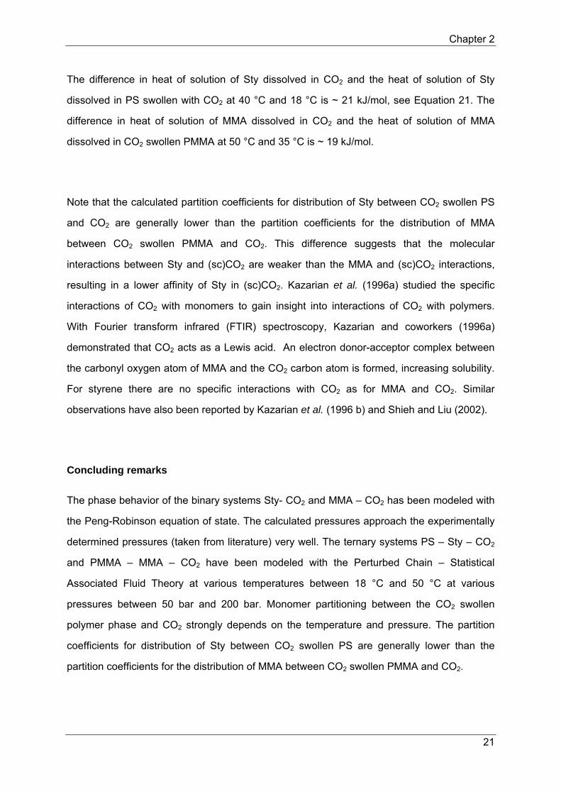
For both the Sty-(sc)CO2 as well as the MMA-(sc)CO2 system it is observed that the
monomer solubility in CO2 decreases with increasing temperature, i.e. at higher
temperatures, a higher pressure is needed to obtain a homogeneous mixture, see Figure 5.
The relation between solubility and pressure is expressed in Equation 1.
y ∗ P γ ∗ x ∗ P (1)
Figure 5a illustrates the solubility of Sty and MMA in CO2 at 35 °C, Figure 5b at 60 °C. Only
the experimentally obtained data points are shown in the figures.
Figure 5 Phase separation pressure of Sty and MMA in (sc)CO2 at 35 °C (a) and 60 °C (b). Open symbols represent Sty, solid symbols represent MMA.
0.6 0.7 0.8 0.9 1.0
90
100
0.6 0.7 0.8 0.9 1.0
60
70
wCO
2
[-]
ba
P [
ba
r]
wCO
2
[-]

Chapter 3
39
The results in Figure 5 demonstrate that Sty-(sc)CO2 isotherms are shifted to higher
pressures than MMA-(sc)CO2 isotherms. This behavior suggests that the molecular
interactions between Sty and (sc)CO2 are weaker than the MMA and (sc)CO2 interactions,
resulting in a lower solubility of Sty in (sc)CO2. Kazarian et al. (1996a) studied the specific
interactions of CO2 with monomers to gain insight into interactions of CO2 with polymers.
With Fourier transform infrared (FTIR) spectroscopy, Kazarian et al. (1996a) demonstrated
that CO2 acts as a Lewis acid. An electron donor-acceptor complex between the carbonyl
oxygen atom of MMA and the CO2 carbon atom is formed, increasing solubility. Styrene does
not possess a carbonyl oxygen atom and therefore no strong Lewis acid-base interactions
with CO2 exist. Other authors reported similar observations (Kazarian et al., 1996 b, Shieh
and Liu, 2002).
The difference in solubility of Sty and MMA in CO2 is also explained by Equations 2 and 3
(DeVoe, 2001), see also Figure 6. Note that Equation 3 follows from Equation 2 using the
Gibbs-Helmholtz relation with temperature independent heats of solution.
Figure 6 schematic representation of a monomer/CO2 mixture.
The monomer distribution coefficient, i.e. the ratio of the monomer weight fraction in the
vapor phase and the monomer weight fraction in the liquid phase, is expressed in terms of
Gibbs free energies of solution, see Equation 2.
Kmon e‐∆∆Gsolution
R*T (2)
ln ∆∆ ∗ (3)

Chapter 3
40
The change in the heat of solution for a monomer solved in CO2 at constant pressure is
calculated through the partition coefficient (Kmon) of the monomer between the liquid and the
vapor phase at a certain temperature. Figure 7 shows the relation between the partition
coefficient and the temperature for both Sty-CO2 (solid symbols) and for MMA-CO2 (open
symbols) at 65.5 bar. The data points calculated from experimentally determined
compositions have been collected in Appendix E.
Figure 7 Partition coefficients for the distribution of monomer over the liquid phase and the vapor phase versus temperature at 65.5 bar. Open symbols represent Sty, solid symbols
represent MMA. Data points are fitted to ln KmonT ‐ ∆∆HsolutionR
1
Tconstant with
Kmon wmonvapor
wmonliquid.
The difference in heat of solution (Hsolution=Hsolution (CO2)-Hsolution (CO2 swollen polymer))
for Sty dissolved in CO2 is ~ - 38 kJ/mole, whereas for MMA this difference is ~ - 60 kJ/mole.
2.9 3.0 3.1 3.2 3.3 3.4-6.0
-5.5
-5.0
-4.5
-4.0
-3.5
-3.0
-2.5
-2.0
ln K
mon
[ k
g m
on/
kg C
O2
]
1/T [10-3/K]

Chapter 3
41
Monomer partitioning over CO2 swollen polymer and scCO2
The monomer partitioning between CO2 swollen polymer and (sc)CO2 has been determined
at 100, 140 and 180 bar at 35, 45 and 60 °C, by adding 10000 ppm and 100 ppm monomer.
The amount of 104 ppm and 100 ppm monomer to be added to the polymer/CO2 mixture has
been chosen to verify if the partition coefficient for distribution of monomer between CO2-
swollen polymer and (sc)CO2 remains constant at the same conditions of temperature and
pressure even when the amount of monomer present decreases. 100 ppm has been chosen
as the experimental lower limit as it becomes more difficult to add an accurate amount of
monomer when the amount to add decreases. While analyzing the CO2 rich phase when only
100 ppm of monomer was added to the system, the resulting concentration of monomer in
CO2 was found to be much higher than 100 ppm. This result suggests that the received PS
and PMMA polymer contain residual monomer. By means of several experiments and some
iterations (see Appendix F) it was found that in the PS granules (~5 mm) about 500 ppm
styrene and in the smaller PS beads (~1 mm) about 2600 ppm styrene was left after
polymerization; in the PMMA beads (~0.5 mm) about 800 ppm residual MMA was found.
Monomer partitioning between the polymer particles and (sc)CO2 is expressed in the partition
coefficient:
K
(4)
Figure 8a shows the results for the determination of the monomer partition coefficient for Sty-
PS-(sc)CO2, Figure 8b graphically represents the results for MMA-PMMA-(sc)CO2. The
phase ratio is in the range 0.035 to 0.045 g polymer/g CO2. Both cases for the addition of
approximately 10000 ppm and 100 ppm of monomer are included.

Chapter 3
42
Figure 8 Partition coefficient for distribution of styrene between (sc)CO2 and PS (a, open symbols) and for distribution of MMA between (sc)CO2 and PMMA (b, solid symbols). , 35 °C, , 45 °C, , 60 °C.
For 100 bar the partition coefficient of Sty at 35 and 45 °C shows an unexpected deviation
(Appendix F). At higher pressures the partition coefficient has an approximately constant
value of 2 [kg PS/ kg CO2]. The same results were obtained for a total of 10000 ppm and for
approximately 3000 ppm (vide supra) styrene in the system. Also the particle diameter size
did not influence the outcome. The partition coefficient of MMA between PMMA and (sc)CO2
is ~0.3 [kg PMMA/kg CO2] for every combination of pressure and temperature analyzed. The
partition coefficients for 10000 ppm and approximately 1000 ppm (vide supra) MMA in the
PMMA/(sc)CO2 mixture are equal.
Theoretical predictions of the partition coefficient with the Perturbed Chain - Statistical
Association Fluid Theory (PC-SAFT) eos, see Chapter 2, and the work of Görnert and
Sadowski (2007 and 2008) suggest that the partition coefficient depends on the (sc)CO2
100 120 140 160 1800
0.2
0.4
0.6
0.8
1.0
100 120 140 160 1800
5
10
15
20
25
30
K M
MA
[ kg
PM
MA
/ kg
CO
2 ]
P [bar]
b: MMA/PMMAa: styrene/PS
K
Sty [
kg
PS
/ kg
CO
2 ]
P [bar]

Chapter 3
43
density and on the solubility of the monomer in the (sc)CO2 phase. The higher the density of
the (sc)CO2 phase, the higher the partition coefficient. The more soluble monomer (MMA)
partitions more towards the (sc)CO2 than the less soluble monomer (Sty). The experimental
values of the partition coefficient in the present work neither show a significant dependence
on (sc)CO2 density, nor show the expected influence of monomer affinity for (sc)CO2, i.e. the
partition coefficient of Sty between PS and (sc)CO2 is found to be higher than the partition
coefficient of MMA between PMMA and (sc)CO2.
The density profile of CO2, see Figure 9, demonstrates that at low pressures CO2 behaves
more gas-like. The binary phase diagrams Sty-CO2 (Figure 3) and MMA-CO2 (Figure 4) also
show a large miscibility gap between monomer and CO2 in the lower pressure region, i.e. low
solubility.
Figure 9 CO2 density profile as a function of pressure for several temperatures. 25 °C, 35 °C, 45 °C, 50 °C, 60 °C, 70 °C, 80 °C, 90 °C; data are calculated with the Modified-Webb-Benedict-Ruben equation of state (Poling et al., 2001).
0 50 100 150 2000.0
0.2
0.4
0.6
0.8
1.0
CO
2 d
en
sity
[g/m
l]
P [bar]

Chapter 3
44
At moderate pressures the CO2 density increases rapidly with increasing pressure, especially
for temperatures lower than 60 °C. At the same time the “solvency ability” of CO2 increases
with increasing pressure. Hence, more monomer dissolves in the CO2 phase. At high
pressures, CO2 becomes more liquid-like, making its density and solubility behavior less
sensitive to pressure changes. Increasing temperature decreases the CO2 density and
“solvency ability”, i.e. less monomer uptake. On the other hand, higher temperatures improve
the monomer volatility, increasing the driving force for monomer uptake by CO2. The
experimental results demonstrate that the latter two effects rule each other out in the higher
pressure region, keeping the partition coefficient approximately independent of pressure.
Although Wu et al. (2002) found different values for the distribution coefficient of Sty between
PS and CO2, these authors reported similar findings about the constancy of the value with
increasing pressure and temperature.
A second issue is that both Görnert and Sadowski (2007, 2008) and Wu et al. (2002) perform
their measurements with annealed polymers, i.e. the polymer product is heated above the
glass transition temperature to remove so-called history effects. By heating the polymer
above the Tg, build-in defects and specific characteristics introduced by the preparation
method of the polymer disappear and a smooth polymer product is obtained. The databank
used in the PC-SAFT modeling is also based on the characteristics of annealed polymers to
calculate its parameters. Already in the seventies of the previous century, van de Ven (1975)
emphasized the influence of history effects in analyzing polymer products, describing
colloidal interactions. Huvard et al. (1980) reported about the influence of annealing poly
acrylonitrile (PAN) on CO2 sorption. Huvard et al. (1980) observed that the sorption capacity
of glassy PAN microspheres decreased by ~30% after annealing the microspheres in
comparison to the “as made” microspheres. The author refers to Koros et al. (1978) and to
Chan et al. (1978) who observed similar effects in CO2 sorption in poly(ethylene terephtalate)
and in polycarbonate, respectively. In the present work the polymers are used as received
from industry, without annealing the product.
A third aspect concerns a possible explanation why the experimentally determined partition
coefficient for Sty is higher than that for MMA, while the theory predicted it the other way
around. Polymers can form physical or entangled networks including ion bridging from one

Chapter 3
45
chain to another and hydrophobic and hydrophilic bonding (Goodwin and Hughes, 2008).
Entanglements in amorphous polymers refer to the degree of topological constraint on the
relative chain motion. An amorphous polymer, both in the glassy and rubbery state can often
be idealized as a network of entangled strands linked at entanglement points. The
entanglement network is characterized by, for example, the density of the entanglement
points (Teerenstra et al., 2003). Teerenstra et al. (2003) pointed out that not only the chain
flexibility is important for the entanglement density, but also the chain diameter plays a
significant role. These authors observed that a larger chain diameter decreases the
entanglement density. The phenyl side groups of PS are larger than the alkyl groups of
PMMA. Bucknall (2001) found that the degree of ductility of a polymeric material also
depends on the entanglement density, both decreasing from polycarbonate to
polyvinylchloride to PMMA to PS. For PS 1.35 bonds per nm3 are counted, for PMMA 1.50
bonds per nm3. Meijer et al. (2000) also reported an increase of the entanglement density
from PS to PMMA. The findings of the authors mentioned are applicable to polymer films,
polymer melts and diluted polymer samples. High-pressure CO2 acts as a plasticizing agent,
swelling the polymer, thereby decreasing the volume fraction of the polymer. The glass
transition temperature of the polymer also decreases changing the polymer from the glassy
to the rubbery state. The plasticization, characterized by increased segmental motion, chain
mobility and inter-chain distance, is largely determined by polymer-solvent interactions and
solvent size (Kazarian, 2000). As mentioned earlier, PMMA and (sc)CO2 form an electron
donor-acceptor complex (Kazarian et al., 1996a) which results in an additional network link
decreasing the distance between entanglements, i.e. increasing the entanglement density
(Goodwin and Hughes, 2008, Brown, 2001). Therefore it is believed that it is easier to extract
Sty from PS than MMA from PMMA due to the higher entanglement density of PMMA.
The same partitioning experiments as presented in Figure 8 have been performed with
polymer beads equilibrated with water. The polymer beads were completely immersed in
demineralized water for several days. Before the experiment started, the water attached to
the surface of the polymer particles was removed. The results for monomer partitioning
between polymer equilibrated with water and (sc)CO2 and those between dry polymer and
(sc)CO2 are not significantly different. There exists no influence of traces of water in the
polymer phase on the monomer partitioning between CO2-swollen polymer and scCO2.

Chapter 3
46
Concluding remarks
A high-pressure optical cell and a high-pressure autoclave have been used to determine the
binary phase behavior for Sty-CO2 and for MMA-CO2. The optical cell as well as the high-
pressure autoclave are found to provide accurate results. In the high-pressure autoclave the
monomer partition coefficients for distribution of monomer between CO2-swollen polymer
particles and (sc)CO2 have been experimentally determined at various pressures between
100 and 180 bar at various temperatures between 35 and 60 °C. The experimental results
demonstrate the partition coefficient is approximately independent of pressure and
temperature. For Sty-PS-(sc)CO2 a partition coefficient of 2 [kg PS/kg (sc)CO2] is found for
the different combinations of pressure and temperature, for MMA-PMMA-(sc)CO2 a value of
0.3 [kg PMMA/kg (sc)CO2] is observed.

Chapter 3
47
References
M. Akgün, D. Emel, N. Baran, N. A. Akgün, S. Deniz, S. Dinçer, “Styrene-carbon dioxide phase equilibria at high pressures”, J. Supercritical Fluids, 2004, 31, 27-32
H. R. Brown, “Relation between the width of an interface between two polymers and its toughness”, Macromol., 2001, 34, 11, 3720-3724
C. B. Bucknall, “Blends containing core-shell impact modifiers Part 1: Structure and tensile deformation mechanisms”, Pure Appl. Chem., 2001, 73, 6, 897-912
A. H. Chan, D.R. Paul, “Effect of sub -Tg annealing on CO2 sorption in polycarbonate”, ACS Preprints, 1978, 39, 230
H. DeVoe, “Thermodynamics and Chemistry”, 2001, Prentice Hall, New York
J. W. Goodwin, R. W. Hughes, “Rheology for chemists: An introduction”, 2nd new ed., 2008, Royal Society of Chemistry, Cambridge
M. Görnert, G. Sadowski, “Phase-equilibrium measurements of the polystyrene/styrene/carbon dioxide ternary system at elevated pressures using ATR-FTIR spectroscopy”, Macromol. Symp., 2007, 259, 236-242
M. Görnert, G. Sadowski, “Phase-equilibrium measurement and modeling of the PMMA/MMA/carbon dioxide ternary system”, J. Supercritical Fluids, 2008, 46, 218-225
G. S. Huvard, V. T. Stannett, W. J. Koros, H. P. Hopfenberg, “The pressure dependence of CO2 sorption and permeation in poly(acrylonitrile)”, J. of Membrane Sci., 1980, 6, 185-201
S. G. Kazarian, C. A. Eckert, J. C. Meredith, K. P. Johnston, J. M. Seminario, “Quantitative equilibrium constants between CO2 and Lewis bases from FTIR spectroscopy”, J. Phys. Chem., 1996 (a) , 100, 10837-10848
S. G. Kazarian, M. F. Vincent, F. V. Bright, C. L. Liotta, C. A. Eckert, “Specific intermolecular interaction of carbon dioxide with polymers”, J. Am. Chem. Soc., 1996 (b), 118, 1729-1736
S. G. Kazarian, “Review: Polymer processing with supercritical fluids”, Polym. Sci., Ser. C, 2000, 42, 78-101
W. J. Koros, D. R. Paul, “CO2 sorption in poly(ethylene terephthalate) above and below the glass transition temperature”, J. Polym. Sci., Polym. Phys. Ed., 1978, 16, 1947
K.-M. Krüger, G. Sadowski, “Fickian and non-fickian sorption kinetics of toluene in glassy polystyrene”, Macromol., 2005, 38, 8408-8417
M. Lora, M. A. McHugh, “Phase behavior and modeling of the poly(methyl methacrylate)-CO2-methyl methacrylate system”, Fluid Phase Eq., 1999, 157, 285-297
H. E. H. Meijer, L. E. Govaert, R. J. M. Smit, “A multi-level finite element method for modeling rubber-toughened amorphous polymers” in R. A. Pearson, H. –J. Sue, A. F. Yee (Eds.) “Toughening of plastics: advances in modeling and experiments”, 2000, American Chemical Society, Washington D. C.
B. E. Poling, J. M. Prausnitz, J. P. O’Connell, “The properties of g ases and liquids”, 5th ed., 2001, The McGraw-Hill Companies, Inc., USA

Chapter 3
48
M. S. da Silva, M. Temtem, S. Henriques, T. Casimiro, A. Aguiar-Rocardo, “Phase behavior studies of 2-hydroxylethyl methacrylate and methyl methacrylate in high-pressure carbon dioxide”, J. Chem. Eng. Dat., 2007, 52, 5, 1970-1974
Y.-T. Shieh, K.-H. Liu, “Solubility of CO2 in glassy PMMA and PS over a wide pressure range: the effect of the carbonyl groups”, J. Polym. Res., 2002, 9, 107-113
G. J. Suppes, M. McHugh, “Phase behavior of the carbon dioxide-styrene system”, J. Chem. Eng. Dat., 1989, 34, 310-312
C.-S. Tan, S.- J. Yarn, J.- H. Hsu, “Vapour-liquid equilibria for the systems carbon dioxide-ethylbenzene and carbon dioxide-styrene”, J. Chem. Eng. Dat., 1991, 36, 23-25
M. N. Teernestra, P. A. M. Steeman, W. Iwnes, A. Vandervelden, D. R. Suwier, B. Van Mele, C. E. Koning, “On the entanglement density of differently N-substituted styrene-maleimide copolymers”, e-Polym., 2003, 045, 1-12
N. I. Uzun, M. Akgün, N. Baran, S. Deniz, S. Dinçer, “Methyl methacrylate plus carbon dioxide phase equilbria at high pressures”, J. Chem. Eng. Dat., 2005, 50, 4, 1144-1147
T. G. M. van de Ven, PhD thesis, 1975, McGill University, Montreal, Canada
J. Wu, Q. Pan, G. L. Rempel, “High pressure phase equilibria for a styrene/CO2/polystyrene ternary system”, J. Appl. Polym. Sci., 2002, 85, 1938-1944
J. Zhang, L. Gao, X. Zhang, B. Zong, T. Jiang, B. Han, “Phase behaviors, density, and isothermal compressibility of styrene + CO2, ethylbenzene + CO2, and ethylbenzene + styrene+ CO2 systems”, J. Chem. Eng. Data, 2005, 50, 1818-1822
G. Zwolak, L Lioe, F. P. Lucien, ”Vapor-liquid equilibria of carbon dioxide plus methyl methacrylate at 308, 313, 323 and 333 K”, Ind. Eng. Chem. Res., 2005, 44, 1021-1026

Chapter 3
49
Appendix A
Concentration time history of monomer in CO2, Figure A.1.a shows the profile for Sty in CO2
at 35 °C and 100 bar, Figure A.1.b for MMA in CO2. After about 2 hours the equilibrium
concentration is set.
Figure A. 1 Concentration profile of a) Sty in CO2 and b) MMA in CO2.
Krüger and Sadowski (2005) studied the sorption kinetics of toluene in glassy polystyrene.
Krüger reported the toluene mass uptake in polystyrene films of thicknesses between 20 and
100 μm at 100 °C while increasing the pressure from 0-400 mbar. The resulting curves show
that sorption of toluene in polystyrene is very slow and can take several days or weeks
before equilibrium is reached.
The reason equilibrium in this work is reached rather fast, only 2 hours, is ascribed to the
preparation of the polymer samples. Krüger and Sadowski (2005) made the polymer films by
increasing the polymer temperature above its glass transition temperature, thereby removing
all influences of the polymerization process. In the present work the polymer particles are
0 2 4 6 8 10 12 140
2
4
6
8
10
12
14
16
18
0 2 4 6 8 10 12 14 160
2
4
6
8
10
12
14
16
mo
le S
ty/
m3 C
O2
time [hr]
ba
mo
le M
MA
/ m3 C
O2
time [hr]

Chapter 3
50
used as received as it is this kind of polymer that in general is the reactor product applied in
industry.

Chapter 3
51
Appendix B
Figure B.1 and B.2 show the calibration plots of the peak area in the chromatogram as a
function of the amount of moles CO2 injected. The calibration has been described with two
separate equations due to the behavior of CO2. Up till an amount of 1.3 ∗ 10-5 moles CO2
injected, the resulting plot can be described with an exponential function, see Equation B.1.
y p 1 ∗e ∗ (B.1)
where p(1) and p(2) stand for the coefficients fitted to the plot (p(1) = 6.17 * 10-6 and p(2) =
0.24 * 10-6 respectively).
Figure B.1 Peak area as a function of the amount of moles CO2 injected (<1.3 ∗ 10-5 moles CO2) into the gas chromatograph. The open symbols represent the measured peak areas of an accurately known amount of moles CO2 injected. The solid line represents the calibration
line fitted to the data, y p 1 ∗ e ∗
Once the amount of moles CO2 injected surmounts 1.3 ∗10-5 moles CO2, the measured data
points have been found to show a linear relation between the peak area and the amount of
moles CO2 injected, see Equation B.2 and Figure B.2.
4 5 6 7 8 9 10 11 12
x 106
1
2
3
4
5
6
7
8
9x 10
-5
amou
nt o
f mol
es C
O2
inje
cted
[10-5
mol
es]
area [106 μm²]

Chapter 3
52
y p 1 p 2 *x (B.2)
where p(1) and p(2) stand for the coefficients fitted to the plot (p(1) = ‐0.35 ∗10-4 and p(2) =
1.1∗10-11 respectively).
Figure B.2 Peak area in function of the amount of moles CO2 injected (>1.3 ∗ 10-5 moles CO2) into the gas chromatograph. The open symbols represent the measured peak areas of an accurately known amount of moles CO2 injected. The solid line represents the calibration line fitted to the data, y p 1 p 2 *x
0 0.5 1 1.5 2 2.5 3 3.5 4 4.5 5
x 106
0
0.2
0.4
0.6
0.8
1
1.2
1.4x 10
-5
amou
nt o
f mol
es C
O2
inje
cted
[10-5
mol
es]
area [106 μm²]

Chapter 3
53
Appendix C
Experimentally determined cloud-points of Sty-(sc)CO2 and MMA-(sc)CO2 at 35, 45 and 60
°C are presented in Table C.1.a and C.2.a respectively. The pressure is the calculated mean
of all the experiments at one condition the standard deviation. Liquid and gas phase
compositions of Sty-(sc)CO2 at 35 °C and of MMA-(sc)CO2 at 45 °C are collected in Table
C.1.b and C.2.b. The weight fraction of (sc)CO2 is the calculated mean of all the experiments
at one condition the standard deviation.
Table C.1.a Cloud-point data of Sty-(sc)CO2
P [bar] at 35 °C P [bar] at 45 °C P [bar] at 60 °C
0.98 72.4 0.8 87 4 101 1
0.89 827 1 104 1
0.86 69 2 80 2 104 2
0.81 68 2 81 3 104 1
0.69 66 2 78 1 99 2
Table C.1.b Liquid and gas phase compositions of Sty-(sc)CO2 at 35 °C
P [bar] at 35 °C in the liquid phase in the gas phase
72 0.934 0.008 0.995 0.0017
70 0.829 0.034 0.994 0.0004

Chapter 3
54
Table C.2.a Cloud-point data of MMA-(sc)CO2
P [bar] at 35 °C P [bar] at 45 °C P [bar] at 60 °C
0.94 68 0.3 80 0.3 97 0.9
0.87 6 0.5 77 0.6 96 0.1
0.85 64 0.4 74 0.4 94 0.4
0.76 60 0.5 71 0.5 91 0.3
Table C.2.b Liquid and gas phase compositions of MMA-(sc)CO2
P [bar] at 45 °C in the liquid phase in the gas phase
82.5 0.94 0.0002 0.95 0.0007
81 0.84 0.0014 0.96 0.0002
73 0.68 0.0005 0.97 0.0001
71 0.63 0.0007 0.97 0.00004

Chapter 3
55
Appendix D
Tables D.1 and D.2 show the vapor-liquid equilibria of Sty-CO2 and of MMA-CO2 at 35 °C, 45
°C and 60 °C respectively. The composition of the liquid phase [L] is weighed into the
equilibrium cell. The vapor phase [V] composition is calculated with the Peng-Robinson
Equation of State, with a binary interaction parameter of 0.046 for Sty-CO2 (Suppes and
McHugh, 1989) and 0.033 for MMA-CO2 (Zwolak et al., 2005). Table D.3 gives the pure
component parameters used in the Peng-Robinson eos.
Table D.1.a Vapor-liquid equilibria of Sty-CO2 at 35 °C.
P [bar] wSty [L] wSty [V] calc wCO2 [V] calc K K
72.4 0.02 0.003 0.997 0.12 1.03
68.9 0.14 0.008 0.992 0.06 1.16
68.1 0.19 0.007 0.993 0.04 1.23
65.5 0.31 0.007 0.993 0.22 1.43
Table D.1.b Vapor-liquid equilibria of Sty-CO2 at 45 °C
P [bar] wSty [L] wSty [V] calc wCO2 [V] calc K K
86.9 0.02 0.003 0.997 0.13 1.02
81.7 0.11 0.003 0.997 0.03 1.12
80.4 0.14 0.003 0.997 0.02 1.16
80.9 0.19 0.003 0.997 0.015 1.23
77.5 0.31 0.004 0.996 0.013 1.44
Table D.1.c Vapor-liquid equilibria of Sty-CO2 at 60 °C
P [bar] wSty [L] wSty [V] calc wCO2 [V] calc K K
101.3 0.02 0.01 0.989 0.43 1.01
103.6 0.11 - - 0.02 1.09
103.5 0.14 - - 0.015 1.12
103.9 0.19 - - 0.007 1.17
99.2 0.31 0.001 0.999 0.003 1.43
Chapter 3
56
Table D.2.a Vapor-liquid equilibria of MMA-CO2 at 35 °C
P [bar] wSty [L] wSty [V] calc wCO2 [V] calc K K
68.4 0.06 0.009 0.991 0.15 1.05
65.6 0.13 0.014 0.986 0.10 1.10
64.3 0.15 0.015 0.985 0.09 1.13
60.2 0.24 0.016 0.984 0.06 1.2
Table D.2.b Vapor-liquid equilibria for MMA-CO2 at 45 °C
P [bar] wSty [L] wSty [V] calc wCO2 [V] calc K K
79.6 0.06 0.015 0.985 0.25 0.95
76.7 0.13 0.014 0.986 0.11 0.88
74.7 0.15 0.014 0.986 0.09 0.86
71.4 0.24 0.013 0.987 0.05 0.77
Table D.2.c Vapor-liquid equilibria for MMA-CO2 at 60 °C
P [bar] wSty [L] wSty [V] calc wCO2 [V] calc K K
96.7 0.06 0.014 0.986 0.23 1.05
95.7 0.13 0.014 0.986 0.11 0.88
94 0.15 0.015 0.985 0.10 0.86
90.0 0.24 0.015 0.985 0.06 0.77
Table D.3 Peng-Robinson parameters as used for calculations. Pure component parameters are taken from Poling et al. (2001), binary interaction parameter kij taken from Suppes and McHugh (1989) and Uzun et al. (2005)
parameter Sty MMA CO2
Tc [K] 647.05 563.95 304.25 Pc [105 Pa] 39.9 36.8 73.8
ω [-] 0.257 0.317 0.225
kSty‐CO2 0.046 kMMA‐CO2 0.033

Chapter 3
57
Appendix E
Tables E.1 and E.2 give the vapor-liquid composition data for Sty-CO2 and for MMA-CO2
respectively, at 65.5 bar at different temperatures, calculated with the Peng-Robinson
Equation of State. The partition coefficient is defined as the ratio of the monomer
concentration in the vapor phase (y) over the monomer concentration in the liquid phase (x),
i. e. Kmon y
x. For the pure component parameters used in the Peng-Robinson eos, see
Table D.3.
Table E.1 Vapor-liquid composition of Sty-CO2 at 65.5 bar and 35, 45 and 60 °C
35 °C 45 °C 60 °C
wSty (x) wSty (y) KSty wSty (x) wSty (y) KSty wSty (x) wSty (y) KSty
0.31 0.007 0.02 0.63 0.006 0.009 0.67 0.005 0.007
Table E.2 Vapor-liquid composition of MMA-CO2 at 65.5 bar and 35, 45 and 60 °C
35 °C 45 °C 60 °C
wMMA (x) wMMA (y) KMMA wMMA (x) wMMA (y) KMMA wMMA (x) wMMA (y) KMMA
0.13 0.01 0.11 0.40 0.01 0.03 0.54 0.01 0.01

Chapter 3
58
Appendix F
Experimentally determined monomer partition coefficient between polymer and CO2. Table
F.1 represents the results for Sty-PS-(sc)CO2, Table F.2 shows the results for MMA-PMMA-
(sc)CO2.
Table F.1 Partition coefficient of Sty between PS and (sc)CO2 [ kg PS/ kg (sc)CO2]
P [bar] K at 35 °C K at 45 °C K at 60 °C
100 18 10 9 2.2 1.8 0.1
140 2 2.5 0.1 1.40 0.01
180 1.0 1.8 0.3 1.00 0.02
Table F.2 Partition coefficient of MMA between PMMA and (sc)CO2 [kg PMMA/ kg (sc)CO2]
P [bar] K at 35 °C K at 45 °C K at 60 °C
100 0.29 0.002 0.25 0.02 0.24 0.01
140 0.38 0.01 0.29 0.02 0.32 0.01
180 0.35 0.01 0.3 0.02 0.28 0.01
The partition coefficient for the distribution of monomer between CO2 swollen polymer and
CO2 has been calculated with Equation F.1
molmon polymer
molmon CO2 (F.1)
The monomer concentration in the polymer phase followed from a mass balance of the
monomer, see Equation F.2.
molmon added molmon CO2 molmon polymer (F.2)
The amount of moles of monomer added to the autoclave was accurately known (see section
‘Materials and methods’). The monomer concentration in the (sc)CO2 phase was measured.
Without any addition of monomer to the polymer, the analysis of the (sc)CO2 showed that

Chapter 3
59
there was already monomer present in the polymer. The calculated partition coefficient, see
Equation F.1, was set as starting value in the determination of the amount of monomer
present in the polymer phase. The newly found number of monomer in the polymer phase
was then added to the number found from the measurement and a new partition coefficient
was determined. This iteration was repeated until a constant value for the partition coefficient
had been found.


61
Chapter 4
Mass transport phenomena in the supercritical carbon dioxide
extraction of residual monomer from latex products
Abstract
The mechanism of mass transport involved in the extraction of residual monomer from a
latex product with supercritical carbon dioxide (scCO2) has been studied. Monomer transport
was found to be governed by the shuttle effect, based on Brownian motion of the polymer
particles to and from the water/scCO2 interface. Surface Gibbs free energy considerations
were used to predict the position of the particles at the (sc)CO2/H2O interface. The main
resistance against monomer transfer from the polymer particles to the (sc)CO2 phase has
been demonstrated to be located inside the polymer particles.
Introduction
Latex is a colloidally stable dispersion of submicron (~100 nm) polymer particles in water.
The polymer particles contain residual monomer due to incomplete conversion. Supercritical
or high-pressure carbon dioxide ((sc)CO2) has been studied as extraction medium to reduce
the residual monomer level in polymer based products. The present work focuses on the
monomer transport mechanism from the submicron polystyrene or polymethyl methacrylate
particles to the (sc)CO2 phase.
Two mechanisms for transfer of monomer from latex particles to (sc)CO2 operate in parallel.
The resistance in series approach, i.e. solid-to-liquid-to-fluid (SLF) mass transfer, as well as
a direct solid-to-fluid (SF) mass transfer model, also referred to as the shuttle effect
(Beenackers and van Swaaij, 1993, Vinke et al., 1993).

Chapter 4
62
In the resistance in series approach, the monomer diffuses out of the polymer particles
through the water (H2O) phase into the (sc)CO2 phase. The main resistance against mass
transfer is located in the H2O phase due to the low monomer solubility (Zhang and Ray,
1997), Figure 1.
Figure 1 The resistance in series mass transport approach. Cmon is the monomer concentration in the respective phases.
Describing the diffusion of monomer through the three phases, i.e. the polymer particles, the
H2O phase and the CO2 phase, the film model has been used. The overall molar mass
transfer flux of the monomer (ϕmon ) is expressed in Equation 1.
ϕmon
∗ /
∗ /
∗ a ∗
∗ C / ∗ / (1)
where kmi , Kmoni/j and aP stand for the monomer mass transfer coefficient in phase i, the
monomer partition coefficient between phase i and phase j and the specific mass transfer
area of the polymer particles, respectively.
In the SF mass transfer approach, the polymer particles move through the H2O phase
towards the H2O/CO2 interface. The monomer diffuses out of the polymer particles directly
into the (sc)CO2 phase, see Figure 2.

Chapter 4
63
Figure 2 The solid-to-fluid mass transfer approach (shuttle mechanism).
The dimension of the polymer particles, allows for Brownian motion in water and
consequently can reside for some time at the H2O/(sc)CO2 interface (Brilman et al., 1998). At
the H2O/(sc)CO2 interface the polymer particle is in direct contact with the (sc)CO2 phase
allowing direct diffusional transport of the monomer from the polymer particles to the (sc)CO2
phase. Alper et al. (1980) used the boundary layer model to describe mass transfer by the
shuttle effect. After a certain contact time the particles near the interface have lost part of the
initially present monomer. Dumont and Delmes (2003) emphasize that in many situations the
contact time between particle and fluid is so short that the steady-state concentration
gradient of the particles containing film does not have enough time to develop. Therefore,
only unsteady-state models can be used to describe mass transfer.
Concentration leveling of the monomer in the polymer phase is related to time or the Fourier
number, see Equation 2 and Figure 3.
Fo ∗ , (2)

Chapter 4
64
Figure 3 Concentration leveling of the monomer in a polymer particle. rp is the polymer particle radius, C0 the initial monomer concentration in the polymer particle (at tcontact = 0), i.e. just before arriving at the H2O/CO2 interface, Cs the monomer concentration at the polymer particle surface, directly after arriving on the H2O/CO2 interface.
Chon et al. (2005) suggest that the residence time of polymer particles at the H2O/(sc)CO2
interface (tcontact, P) can be regarded in terms of Brownian motion of the polymer particles in
the water phase, see Equation 3. Chon et al. (2005) used Al2O3 nanoparticles to increase
the heat conductivity of water and validated that Brownian motion of the nanoparticles is the
key mechanism for thermal conductivity enhancement. Comparable observations are
reported by other authors (Jang and Choi, 2004). tcontact, P can be described as the ratio of the
length scale of the interfacial region (∆s) and the Brownian velocity of of the polymer
particles (vBr).
t ,p (3)
The length scale of the interfacial region is assumed to be 10 μm (Kemmere et al., 2002); Δ
is of the same order of magnitude. The Brownian velocity (vBr) follows from Equation 4.
v ∗
∗ ∗ ∗ ∗ (4)
where kb stands for the Boltzman constant, η for the water viscosity and lBF for the mean free
path of the particle in water (l = 0.17 nm (Jang and Choi, 2004)).

Chapter 4
65
For Fo < 0.1, mass transport in the polymer particles can be regarded to be in a semi-infinite
medium. Then the penetration theory applies for mass transport, Equation 5 (Welty et al.,
2001, Bird et al., 2002).
k 2 ∗ ∗ ,
(5)
For Fo > 0.1, intraparticle mass transport can be described with Equation 6 (van den Akker
and Mudde, 1997), see Figure 3.
Sh ∗
6.6 (6)
The mass transfer resistance depends on the specific area of the H2O/(sc)CO2 interface.
Joly-Vuillemin and Bellefon (1999) suggest that the polymer particles partially cover the
H2O/(sc)CO2 interface. The effective specific mass transfer area is then defined as:
a SF a ∗ θ for the shuttle effect (7)
a SLF a * 1‐θ for the SLF approach (8)
Note that θmax is 0.74, i.e. the maximum fractional surface coverage by spherical particles in
a three dimensional closest packing.
As mentioned earlier the SLF model is diffusion limited due to the low monomer solubility in
water (Zhang and Ray, 1997). The partitioning of monomer between the particles and the
water phase is very low towards the water phase, K / is in the order of magnitude
of 10-3 kg polymer/kg H2O (Kemmere et al. 2005, González et al., 2007). In comparison with
the SF mass transfer model, phase equilibrium of monomer between the particles and
(sc)CO2 cannot be reached within a short time. The shuttle effect is therefore dominating
the mass transfer. The mass transfer-in-series contribution is assumed to be negligible.
Interfacial properties
Interfacial properties, more specifically interfacial tension between the phases involved is an
important quantity associated with mass transfer. The interfacial tension, related to the
specific interfacial Gibbs energy, is the excess Gibbs energy per unit area due to the

Chapter 4
66
formation of an interface (Van Krevelen, 1997). The interfacial tension is closely related to
the cohesion energy of a system (O’Neill et al., 1998).
In 1907, Pickering observed that solid particles could adhere to a liquid-liquid interface
thereby stabilizing emulsions (Pickering, 1907). Finkle et al. (1923) suggested the emulsions
were stabilized because the particles were partially wetted by the two liquids involved. The
ability of solid particles to adhere to a liquid-liquid interface has been described by Colver et
al. (2006) in terms of energy contributions.
Torza and Mason (1970) reported a thermodynamic approach to predict the morphology of
two immiscible liquids suspended in a liquid immiscible with both other liquids. Based on the
pioneering work of Torza and Mason (1970), numerous authors were able to
thermodynamically predict the morphology of composite latex systems, see e.g. Sundberg et
al. (1990), Chen et al. (1991) and Sundberg and Sundberg (1993).
In all cases reported, the thermodynamically preferred morphology is the one that has the
lowest interfacial Gibbs free energy. The driving force to obtain the preferred morphology at
fixed pressure and temperature, the Gibbs free energy change (∆G) of the process, can be
expressed as (Hiemenz and Rajagopalan, 1997):
∆G ∑ γ ∗ A γ ∗ A (9)
where γi, Ai, γ0 and A0 stand for the interfacial tension of the ith interface and its
corresponding interfacial area, the interfacial tension of the original polymer suspended in
water and the corresponding interfacial area, respectively.
In the present work, the position of polystyrene (PS) and polymethyl methacrylate (PMMA)
latex particles in a biphasic (sc)CO2/H2O environment has been predicted using the theory of
Torza and Mason (1970) as well as the theory of Colver et al. (2006).
Torza and Mason (1970) defined the spreading coefficients (Si) of a three-phase system,
which yields the same result as an analysis based on minimizing the Gibbs free energy, as:
(10)

Chapter 4
67
By convention, phase 1 must be the phase for which , so that S1 < 0. Then
complete engulfment, i.e. core-shell morphology, occurs when S2 < 0 and S3 > 0. If S2 < 0
and S3 < 0, the engulfment is only partial and leads to hemispherical morphologies. When
S2 > 0 and S3 < 0, separated structures are preferred. Removing the restriction that
, a fourth less common morphology can be predicted as a special case of core-shell, i.e.
inverted core-shell, when S1 > 0, S2 < 0 and S3 < 0. Figure 4 shows all possible structures
and their spreading coefficients.
Figure 4 Engulfment and spreading coefficients according to the theory of Torza and Mason (1970).
In the present work, two systems have been investigated; a polystyrene (PS) latex and a
polymethyl methacrylate (PMMA) latex are both submitted to extraction with (sc)CO2.
Interfacial tension between polymer particles and (sc)CO2 decreases with increasing
pressure due to the adsorption of (sc)CO2 at the interface (Jaeger et al., 1996, Otake et al.,
1994).
Table 1 gives the interfacial tensions between H2O and CO2 (Tewes and Boury, 2004,
Owens and Wendt, 1969, da Rocha et al., 2001, Kvamme et al., 2007, Dhanuka et al.,
2006), H2O and polymer (Sundberg et al., 1990, Webber et al., 1997) as well as between
CO2 and polymer at 100 bar and 35 °C, without any surfactant in either phase. The
spreading coefficients are also collected in Table 1. The interfacial tension between CO2 and
polymer has been calculated by fitting data of Otake et al. (2004), who correlated the CO2
density to the interfacial tension between CO2 and PS as well as between CO2 and PMMA.

Chapter 4
68
The spreading coefficients have been calculated according to Torza’s theory (Torza and
Mason, 1970). To fulfill the condition , PS, H2O and CO2 were designated as
phase 1, 2, 3 respectively. In case of PMMA, CO2 was taken as phase 1 and PMMA as
phase 3.
Table 1 Interfacial tensions at 100 bar and 35 °C between H2O and CO2 (Kvamme et al., 2007 et al.), between H2O and polymer (Sundberg et al., 1990, Webber et al., 1997) and between CO2 and polymer (Otake et al., 2004). The spreading coefficients have been calculated with the Torza theory (Torza and Mason, 1970). The systems do not contain surfactant molecules.
Interfacial tensions [mN.m-1] Spreading coefficients
polymer S1 S2 S3
PS 30 5.4 40.1 - 15.5 - 64.7 4.7
PMMA 30 5.1 25.4 - 9.7 - 50.3 - 0.5
The calculated spreading coefficients predict complete wetting of polymer particles in CO2
for PS, i.e. CO2 completely wets the polymer particles, and an intermediate structure, i. e.
the polymer particles are partially wetted by the CO2 and partially by the H2O, for PMMA.
As mentioned before, latex is a dispersion of submicron polymer particles in water,
colloidally stabilized by surface active agents. Surfactants consist of both a hydrophilic part
and a hydrophobic part. Upon addition of a surfactant to a system of two immiscible phases,
the surface active agent is adsorbed at the interface. When the surfactant molecules replace
molecules from the original interface, the interaction across the interface is now between the
hydrophilic group of the surfactant and the polar phase on one side of the interface and
between the hydrophobic group of the surfactant and the apolar phase on the other side of
the interface. The newly formed interactions are much stronger than the original interaction
between the dissimilar polar and apolar molecules, consequently the interfacial tension is
significantly reduced by the presence of the surfactant (Rosen, 2004, Chattoraj, 2001).
Rosen (2004) also compared several surfactants in the performance of reducing the
interfacial tension. Every type of surfactant, i.e. non-ionic, ionic or electrosteric, has a
certain efficiency in adsorbing at the interface between two phases, depending on the

Chapter 4
69
investigated system, thereby decreasing the interfacial tension. Harrison et al. (1996) also
reported about the effect of different surfactants on the interfacial tension between two
phases.
The latex systems investigated in the present work are stabilized by sulfate group containing
surfactants. For simplicity, sodium dodecyl sulfate (SDS) has been chosen as surfactant to
perform the calculations of Torza (Torza and Mason, 1970). Table 2 shows the interfacial
tensions between H2O/SDS and CO2 (Dhanuka et al., 2006), H2O/SDS and polymer
(Sundberg et al., 1990, Sundberg and Sundberg, 1993) and CO2 and polymer, as well as the
spreading coefficients. Otake et al. (2004) reported about the interfacial tension at the
CO2/polymer interface in the presence of tetradecanoic acid (MA), demonstrating the surface
activity of carboxylic surfactants. At the same CO2 density, the interfacial tension between
CO2 and polymer/MA is approximately half the value of the interfacial tension between CO2
and polymer without surfactant. Addition of SDS to the system CO2/polymer will also
decrease the interfacial tension as compared to the system without surfactant. However, due
to the lack of any experimental data, the interfacial tension of the surfactant free system is
used in the calculation of the spreading coefficients.1
In order to fulfill the requirement , polymer, H2O and CO2 were designated as
phase 1, 2 and 3, respectively.
Table 2 Interfacial tensions at 100 bar and 35 °C between H2O/SDS and CO2 (Dhanuka et al., 2006), between H2O/SDS and polymer (Sundberg et al., 1990, Sundberg and Sundberg, 1993) and between CO2 and polymer (Otake et al., 2004). The spreading coefficients have been calculated with the Torza theory (Torza and Mason, 1970). The water systems contain sodium dodecyl sulfate (SDS) as surfactant.
Interfacial tensions [mN.m-1] Spreading coefficients
polymer / / S1 S2 S3
PS 4 5.4 13.2 - 14.6 - 11.8 3.8
PMMA 4 5.1 10.7 - 11.8 - 9.6 1.6
1 The interfacial tension between CO2 and polymer without surfactant is already so small, that using this value instead of the slightly smaller interfacial tension between CO2-polymer/surfactant, does not change the result of the calculation of the spreading coefficients. In both cases, the same morphology has been predicted.

Chapter 4
70
The calculated spreading coefficients predict complete wetting of the polymer particles in
CO2 for both PS and PMMA.
The position of the polymer particles in the CO2/H2O interfacial region predicted by the
theory of Torza (Torza and Mason, 1970) was verified by the Pickering stabilization theory
(Colver et al., 2006). Colver et al. (2006) predict the polymer particle position with respect to
a flat liquid-liquid interface and relative to the centre of the spherical polymer particle defining
a dimensionless number, z0, see Equation 11 and Figure 5.
z (11)
Figure 5 Schematic representation for a sphere at a liquid-liquid interface.
The total Gibbs energy the system experiences is the sum of different energy contributions
of the three interfaces (polymer-phase 1, polymer-phase 2, phase 1-phase 2). Division of the
total Gibbs energy by kb ∗ T, results in the dimensionless total energy of the system, see
Equation 12.
G ∗ ∗
∗ ∗ z 2 ∗ a b ∗ z 2 ∗ a 2 ∗ b 1 (12)
with a γp1γ21
and b γp2γ21
. The minimum energy follows from the first derivative of G0 with
respect to z0, see Equation 13.
2 ∗ z 2 ∗ a b 0 (13)
The equilibrium position of the particle is, see Equation 14.
z b a (14)
There are three possible scenarios:

Chapter 4
71
z 1 the particle will be completely in phase 1
z 1 the particle will be completely in phase 2
1 z 1 the particle will adhere at the interface of phase 1 and 2
The interfacial tensions between polymer and CO2, polymer and H2O as well as between
CO2 and H2O at 100 bar and 35 °C (see also Table 1) are collected in Table 3. These
interfacial tensions have been used in the calculation of the equilibrium position and energy
of the polymer particle following the theory of Colver et al. (2006). CO2 is designated as
phase 1, H2O as phase 2. The system does not contain a surface active agent. The polymer
particles have a diameter of 100 nm.
Table 3 Interfacial tensions at 100 bar and 35 °C between H2O and CO2 (Kvamme et al., 2007 et al.), between H2O and polymer (Sundberg et al., 1990, Webber et al., 1997) and between CO2 and polymer (Otake et al., 2004). The equilibrium position of a polymer particle in a CO2-H2O system at 100 bar and 35 °C and the energy of the system have been calculated with the theory of Colver et al. (2006). There are no surfactants present in the system.
Interfacial tensions [mN.m-1] Equilibrium position of the polymer particle [-] and energy of the system [-]
polymer a b z0 G0 [106]
PS 5.4 40.1 30 0.18 1.34 1.16 38.5
PMMA 5.1 25.4 30 0.17 0.85 0.68 31.9
For PS, the theory of Colver et al. (2006) predicts that the PS particles will be completely
wetted by the CO2 phase (z0 ≥ 1). This result is comparable to the prediction of the position
of the PS in the interfacial region with the theory of Torza and Mason (1970). The PMMA
particles will adhere at the CO2-H2O interface (-1 ≤ z0 ≤ 1) as has also been predicted by the
theory of Torza and Mason (1970).
Table 4 shows the results of analogous calculations using the interfacial tensions between
polymer and CO2, polymer and H2O/SDS as well as between CO2 and H2O/SDS.

Chapter 4
72
Table 4 Interfacial tensions at 100 bar and 35 °C between H2O/SDS and CO2 (Dhanuka et al., 2006), between H2O/SDS and polymer (Sundberg et al., 1990, Sundberg and Sundberg, 1993) and between CO2 and polymer (Otake et al. 2004). The equilibrium position of a polymer particle in a CO2-H2O system at 100 bar and 35 °C and the energy of the system have been calculated with the theory of Colver et al. (2006). The water systems contain sodium dodecyl sulfate (SDS) as surfactant.
Interfacial tensions [mN.m-1] Equilibrium position of the polymer particle [-] and energy of the system [-]
polymer a b z0 G0 [106]
PS 5.4 13.2 4 1.35 3.3 1.95 33.2
PMMA 5.1 10.7 4 1.28 2.68 1.4 36.5
Again the equilibrium position predicted with the theory of Colver et al. (2006) corresponds to
that predicted with the theory of Torza and Mason (1970). Using interfacial tensions given in
Table 4 predicts completely wetted particles with CO2 for polystyrene as well as for
polymethyl methacrylate (z0 ≥ 1).
Interesting is that Colver et al. (2006) suggest that the Gibbs energy necessary to remove
the particle from its equilibrium position has a value in the order of 106*kb*T, meaning that
the polymer particle is irreversibly trapped at its equilibrium position and cannot escape via
simple Brownian motion. Figure 6 clarifies this suggestion graphically for a PMMA particle in
a CO2-H2O system at 100 bar and 35 °C without surfactant. The respective energy barriers
have been calculated according to Equations 15 and 16.
∆G G z 1 G z b a (15)
∆G G z 1 G z b a (16)

Chapter 4
73
Figure 6 Gibbs energy profile of a 100 nm PMMA particle in a CO2-H2O interfacial region at 100 bar and 35 °C, without surfactant.
For the other systems, i.e. a PS particle in a CO2-H2O system at 100 bar and 35 °C without
surfactant, a PMMA particle in a CO2-H2O system at 100 bar and 35 °C with surfactant, a PS
particle in a CO2-H2O system at 100 bar and 35 °C with surfactant, similar graphs are
obtained.
According to the theory of Torza and Mason (1970) as well as the theory of Colver et al.
(2006), when PS or PMMA latex, stabilized with SDS as surface active agent, are
submerged into a (sc)CO2 environment, the polymer particles will be completely wetted by
the (sc)CO2. Moreover, the polymer particles are trapped in the (sc)CO2 phase or in other
words the particles irreversibly move from the H2O phase into the (sc)CO2 phase!
This conclusion has not been confirmed by our experimental observations. In a mixture of a
PS latex, stabilized with SDS, and CO2 at 100 bar and 35 °C, the polymer particles were
“homogeneously” distributed throughout the mixture. No phase separation between the H2O
-1 0 10
50
100
150
200
G1 = 5.8 * 106 [-]
G2 = 156 * 108 [-]
CO2
H2O
G
0 [1
06 -]
z0 [-]

Chapter 4
74
phase and the CO2 phase containing the polymer particles occurred, i.e. flotation of the
polymer particles in the lighter CO2 phase was not observed.
The calculated results have been obtained with interfacial tension data from literature, see
Tables 1-4. The polymer films used in literature were all annealed at temperatures above
their glass transition temperature to exclude any effect of the synthesis method or by
impurities on the result of the measurement. Van de Ven (1975) emphasized the influence of
history effects describing colloidal interactions in a PS latex. Huvard et al. (1980) also
reported about the influence of annealing poly acrylonitrile (PAN) on CO2 sorption. Huvard et
al.(1980) observed that the sorption capacity of glassy PAN microspheres decreased by
~30% after annealing the microspheres. The author refers to Koros and Paul (1978) and to
Chan and Paul. (1978) who observed similar effects in CO2 sorption in poly(ethylene
terephtalate) and in polycarbonate, respectively. It is believed that including history effects
also has a profound effect on interfacial characteristics.
The interfacial tension between H2O containing the surfactant SDS and CO2 decreases with
a factor 8 in comparison to the interfacial tension between surfactant free H2O and CO2, due
to the orientation of the surfactant at the interface. The interactions between the polar part of
the surfactant and H2O on one hand and between the non polar part and CO2 on the other
hand are much stronger than the interactions between H2O and CO2, as explained earlier. In
latex systems, the tail group of the surfactant is oriented inside the polymer particles. When
all surfactant is located on the polymer particles, interaction between H2O and CO2 weakens
in comparison to a surfactant orientation over the H2O/CO2 interface. Note that the polymer
particles are surrounded by an electrical double layer of ions, changing the interaction with
CO2.
In either case of positioning of the polymer particles, i.e. at the H2O/CO2 interface or
completely in the CO2 phase, it should be realized that the particles are so small that the
maximum fractional interface coverage of 74 % is reached.

Chapter 4
75
Mass transfer resistance
In the solid-to-fluid (SF) mass transport approach, i.e. the shuttle effect, monomer diffuses
directly from the polymer particles to the (sc)CO2 phase. The residence time, tcontact,P of one
polymer particle at the H2O/(sc)CO2 interface, calculated with Equations 3 and 4 for 100 nm
particles, is3.8*10‐4s. Within this time monomer is transferred from the polymer to the
(sc)CO2 phase. The overall resistance against mass transfer at the position where the
polymer contacts the H2O/CO2 interface is expressed in Equation 17.
1
k*a overall 1
k*a polymerphase 1
k*a*Kmonpolymer/CO2
CO2phase
(17)
The specific area available for mass transport, a [m2/m3 polymer] , for spherical particles
applies. The partition coefficient Kmonpolymer/CO2 is defined as the ratio of monomer
concentration in the CO2 phase and the monomer concentration in the polymer phase, see
Equation 18.
K
(18)
When it is assumed that the polymer particle contacts the H2O/CO2 at one point, see Figure
7, mass transfer from the polymer particle through the interfacial region to the CO2 phase is
also possible.
Figure 7 Mass transfer from the polymer particle through the interfacial region to the (sc)CO2 phase.
The overall resistance against mass transfer through the interfacial region is expressed in
Equation 19, see also Figure 8.

Chapter 4
76
Figure 8 Concentration profile of monomer in the polymer, water and CO2 phase.
1
k*a overall
1
k*a polymerphase
1
k*a*Kmonpolymer/H2O
H2Ophase
1
k*a*KmonO/CO2
CO2phase (19)
The mass transfer coefficient of monomer in the H2O phase is defined by the film theory, see
Equation 1, averaged over the distance between the particle and the H2O/CO2 interface.
Example
It is assumed that residual monomer from PS latex and from PMMA latex is extracted by
(sc)CO2 in a countercurrent column. Latex has been chosen as the continuous phase,
(sc)CO2 is dispersed as 1 mm bubbles through the latex. Table 5 gives the parameters used
to calculate the mass transfer resistance in each phase. The mass transfer coefficient of
monomer in the polymer phase has been calculated according to Equation 5 (Fo < 0.1), for a
diffusion coefficient of monomer in CO2-swollen polymer of 10 . The concentration
leveling in a 1 mm CO2 bubble, i.e. when Fo = 0.1, requires 7 s; the mass transfer coefficient
of monomer in the CO2 bubble has then been calculated with Equation 5 for CO2 instead of
polymer. The mass transfer coefficient of monomer in water has been calculated for
distances from the H2O/CO2 interface to the surface of the polymer particle of 1 to 10 nm.

Chapter 4
77
Table 5 Parameters used in the prediction of the mass transfer resistance in the polymer particles, -H2O/CO2 interfacial region and in the CO2 bubble at 100 bar and 35 °C. (Kemmere et al., 2005, González et al., 2007)
polymer k
ms
D ms
kms
kms
KmP/H2O kgH2O
kgP Km
H2O/C kgCO2kgH O
PS 7 * 10-5 1.4 * 10-8 5 *10-5 4 * 10-1 3 * 10-3 20 PMMA 7 * 10-5 6.8 * 10-8 2.4 * 10-4 4 * 10-1 1.5 * 10-2 15
The partition coefficients of monomer between the polymer particles swollen with CO2 and
the (sc)CO2 phase have been experimentally determined, see Chapter 3,
KstyPS/CO2 2
kgPS
kgCO2 and K / 0.3
.
Table 6 collects the resulting mass transfer resistances in the polymer as well as in the CO2
phase respectively, see Equation 17. Calculations have been performed including the
specific surface area with relation to the surface area of the CO2 bubble.
Table 6 Time constants for the mass transfer resistance in the polymer and CO2 phase at the contact point of polymer particle and H2O/CO2 interface
polymer 1k*a polymerphase
s 1
k*a*Kmonpolymer/C
CO2 phase
s
PS 2.3 1.67 PMMA 2.3 0.02
Table 6 shows the mass transfer resistance in extraction of residual monomer from PS latex
as well as from PMMA latex with (sc)CO2 is for the major part inside the polymer particles.
Table 7 gives the calculated resistance against mass transfer inside the polymer particle,
through the H2O/CO2 interfacial region as well as in the CO2 bubble not attached to the
polymer particle, see Equation 19.
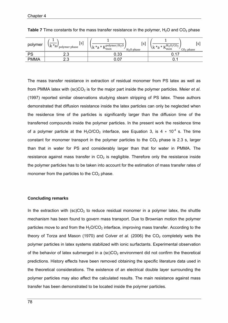
Chapter 4
78
Table 7 Time constants for the mass transfer resistance in the polymer, H2O and CO2 phase
The mass transfer resistance in extraction of residual monomer from PS latex as well as
from PMMA latex with (sc)CO2 is for the major part inside the polymer particles. Meier et al.
(1997) reported similar observations studying steam stripping of PS latex. These authors
demonstrated that diffusion resistance inside the latex particles can only be neglected when
the residence time of the particles is significantly larger than the diffusion time of the
transferred compounds inside the polymer particles. In the present work the residence time
of a polymer particle at the H2O/CO2 interface, see Equation 3, is 4 ∗ 10-4 s. The time
constant for monomer transport in the polymer particles to the CO2 phase is 2.3 s, larger
than that in water for PS and considerably larger than that for water in PMMA. The
resistance against mass transfer in CO2 is negligible. Therefore only the resistance inside
the polymer particles has to be taken into account for the estimation of mass transfer rates of
monomer from the particles to the CO2 phase.
Concluding remarks
In the extraction with (sc)CO2 to reduce residual monomer in a polymer latex, the shuttle
mechanism has been found to govern mass transport. Due to Brownian motion the polymer
particles move to and from the H2O/CO2 interface, improving mass transfer. According to the
theory of Torza and Mason (1970) and Colver et al. (2006) the CO2 completely wets the
polymer particles in latex systems stabilized with ionic surfactants. Experimental observation
of the behavior of latex submerged in a (sc)CO2 environment did not confirm the theoretical
predictions. History effects have been removed obtaining the specific literature data used in
the theoretical considerations. The existence of an electrical double layer surrounding the
polymer particles may also affect the calculated results. The main resistance against mass
transfer has been demonstrated to be located inside the polymer particles.
polymer 1k*a polymerphase
s 1
k*a*Kmonpolymer/H2O
H2Ophase
s1
k*a*KmonO/CO2
CO2phase
s
PS 2.3 0.33 0.17 PMMA 2.3 0.07 0.1

Chapter 4
79
References
H. E. A. van den Akker, R. F. Mudde, E. Stammers, “Fysische transportverschijnselen: 200 vraagstukken”, 1997, 2nd ed., Delft University Press, The Netherlands
E. Alper, B. Wichtendahl, W. D. Deckwer, “Gas absorption mechanism in catalytic slurry reactors”, Chem. Eng. Sci., 1980, 35, 217-222
A. A. C. M. Beenackers, W. P. M. van Swaaij, “Mass transfer in gas-liquid slurry reactors”, Chem. Eng. Sci., 1993, 48, 18, 3109-3139
R. B. Bird, W. E. Stewart, E. N. Lightfoot, “Transport phenomena”,2002, 2nd edition, J. Wiley and sons Inc., New York
D. W. F. Brilman, W. P. M. van Swaaij, G. F. Versteeg, “A one-dimensional instationary heterogeneous mass transfer model for gas absorption in multiphase systems”, Chem. Eng. Process., 1998, 37, 471-488
A. H. Chan, D. R. Paul, “Effect of sub-Tg annealing on CO2 sorption in polycarbonate”, ACS Preprints, 1978, 39, 230
D. K. Chattoraj, “Thermodynamics of adsorption at interfaces and the Gibbs surface excess”, PINSA, 2001, 67A, 6, 663-685
Y-C. Chen, V. Dimonie, M. S. El-Aasser, “ Interfacial phenomena controlling particle morphology of composite latexes”, J. Appl. Polym. Sci., 1991, 42, 1049-1063
Y-C. Chen, V. Dimonie, M. S. El-Aasser, “Effect of interfacial phenomena on the development of particle morphology in a polymer latex system”, Macromolec., 1991, 24, 3779-3787
C. H. Chon, K. D. Kihm, S. P. Lee, S. U. S. Choi, “Empirical correlation finding the role of temperature and particle size for nanofluid (Al2O3) thermal conductivity enhancement”, Appl. Phys. Lett., 2005, 87, 153107
P. J. Colver, T. Chen, S. A. F. Bon, “Supracolloidal structures through liquid-liquid interface driven assembly and polymerization”, Macromol. Symp., 2006, 245-246, 34-41
V. V. Dhanuka, J. L. Dickson, W. Ryoo, K. P. Johnston, “High internal phase CO2-in-water emulsions stabilized with a branched nonionic hydrocarbon surfactant”, J. Colloid Interface Sci., 2006, 298, 406-418
E. Dumont, H. Delmas, “Mass transfer enhancement of gas absorption in oil-in-water systems: a review”, Chem. Eng. Process., 2003, 42, 419-438
P. Finkle, H. D. Draper, J. H. Hildebrand, J. Amer. Chem. Soc., 1923, 45, 12, 2780-2788
L. M. González, O. Suárez-Iglesias, J. L. Bueno, C. Pizarro, I. Medina, “Limiting binary diffusivity of aniline, styrene, and mesitylene in supercritical carbon dioxide”, J. Chem. Eng. Data, 2007, 52, 1286-1290
K. L. Harrison, K. P. Johnston, I. C. Sanchez, “Effects of surfactants on the interfacial tension between carbon dioxide and polyethylene glycol”, Langmuir, 1996, 12, 2637-2544
P. C. Hiemenz, R. Rajagopalan, “Principles of colloid and surface chemistry”, 3th ed., 1997, Marcel Dekker, Inc., New York

Chapter 4
80
G. S. Huvard, V. T. Stannett, W. J. Koros, H. P. Hopfenberg, “The pressure dependence of CO2 sorption and permeation in poly(acrylonitrile)”, J. Membrane Sci., 1980, 6, 185-201
P. T. Jaeger, J. v. Schnitzler, R. Eggers, “Interfacial tension of fluid systems considering the nonstationary case with respect to mass transfer”, Chem. Eng. Technol., 1996, 19, 197-202
S. P. Jang, S. U. S. Choi, “Role of Brownian motion in the enhanced thermal conductivity of nanofluids”, Appl. Phys. Lett., 2004, 84, 21, 4316-4318
C. Joly-Vuillemin, C. Bellefon, “Solids effects on gas-liquid mass transfer in three-phase slurry catalytic hydrogenation of adiponitrile over raney nickel”, Chem. Eng. Sci., 1999, 51, 10, 2149-2158
J-Y. Jung, J. Y. Yoo, “Thermal conductivity enhancement of nanofluids in conjunction with electrical double layer (EDL)”, Int. J. Heat Mass Transfer, 2009, 52, 525-528
M. F. Kemmere, M. Cleven, M. A. van Schilt, J. T. F. Keurentjes, “Process design for the removal of residual monomer from latex products using supercritical carbon dioxide”, Chem. Eng. Sci., 2002, 57, 3929-3937
M. F. Kemmere, M. van Schilt, M. Jacobs, J. T. F. Keurentjes, “Reduction of residual monomer in latex products using high pressure carbon dioxide”, in “Supercritical carbon dioxide in polymer reaction engineering”, M. F. Kemmere, T. Meyer, Eds., 2005, Wiley-VCH, Germany
W. J. Koros, D. R. Paul, “CO2 sorption in poly(ethylene terephtalat) above and below glass transition”, J. Polym. Sci., Polym. Phys. Ed., 1978, 16, 1947
D. W. van Krevelen in “Properties of Polymers”; 3rd Ed., Amsterdam: Elsevier, 1997, Chapter 8
B. Kvamme, T. Kuznetsova, A. Hebach, A. Oberhof, E. Lunde, “Measurements and modeling of interfacial tension for water + carbon dioxide systems at elevated pressures”, Comp. Mat. Sci., 2007, 38, 506-513
D. Meier, H.-J. Warnecke, J. Prüss, “Modelling of mass transfer of volatile organic compounds in polymer dispersions”, Chem. Eng. J. , 1997, 67, 45-53
M. L. O’Neill, Q. Cao, M. Fang, K. P. Johnston, S. P. Wilkinson, C. D. Smith, J. L. Kerschner, S. H. Jureller, “Solubility of homopolymers and copolymers in carbon dioxide”, Ind. Eng. Chem. Res., 1998, 37, 3067-3079
K. Otake, M. Kobayashi, Y. Ozaki, S. Yoda, Y. Takebayashi, T. Sugeta, N. Nakazawa, H. Sakai, M. Abe, “Surface activity of myristic acid in the poly(methyl methacrylate)/supercritical carbon dioxide system”, Langmuir, 2004, 20, 6182-6186
D. K. Owens, R. C. Wendt, “Estimation of the surface free energy of polymers”, J. Appl. Polym. Sci., 1969, 13, 1741-1747
S. U. Pickering, “Emulsions”, J. Chem. Soc. Transactions, 1907, 91, 2001-2021
S. R. P. da Rocha, K. P .Johnston, R. E. Wetsacott, P. J. Rossky, “Molecular structure of the water-supercritical CO2 interface”, J. Phys. Chem. B, 2001, 105, 12092-12104
M. J. Rosen in “Surfactants and interfacial phenomena”; 3rd Ed., New York: John Wiley & sons, Inc., 2004, Chapter 5

Chapter 4
81
D. C. Sundberg, A. P. Cacassa, J. Pantazopoulos, M. R. Muscato, “Morphology development of polymeric microparticles in aqueous dispersions. I. Thermodynamic considerations”, J. Appl. Polym. Sci., 1990, 41, 1425-1442
E. Sundberg, D. C. Sundberg, “Morphology development for three-component emulsion polymers: Theory and experiments”, J. Appl. Polym. Sci., 1993, 47, 1277-1294
F. Tewes, F. Boury, “Thermodynamic and dynamic interfacial properties of binary carbon dioxide-water systems”, J. Phys. Chem. B , 2004, 108, 2405-2412
S. Torza, S. G. Mason, “Three-phase interactions in shear and electrical fields”, J. Colloid Interface Sci., 1970, 33, 1, 67-83
T. G. M. van de Ven, PhD thesis, 1975, McGill University, Montreal, Canada
H. Vinke, P. J. Hamersma, J. M. H. Fortuin, “Enhancement of the gas-absorption rate in agitated slurry reactors by gas-absorbing particles adhering to gas bubbles”, Chem. Eng. Sci., 1993, 48, 12, 2197-2210
J. A. Waters, “Predicting the surface morphology of composite latex particles”, Colloids and Surfaces A: Physicochem. Eng. Aspects, 1994, 83, 167-174
S. E. Webber, P. Munk, K. P. Johnston, K. Otake, “Swelling of polystyrene latex particles in water by high-pressure carbon dioxide”, Langmuir, 1997, 13, 20, 3047-3051
J. Welty, C. E. Wicks, R. E. Wilson, “Fundamentals of momentum, heat, and mass transfer”, 2001, 4th ed., Wiley, Chichester
S. X. Zhang, W. H. Ray, “Modelling and experimental studies of aqueous suspension polymerization processes. 3. Mass transfer and monomer solubility effects”, Ind. Eng. Chem. Res., 1997, 36, 1310-1321


83
Chapter 5
Process design for residual monomer reduction in latex with
supercritical carbon dioxide
Abstract
Processes other than steam stripping or chemical conversion to reduce residual monomer in
latex products are being intensively studied. One of the alternative processes is the
extraction of residual monomer with high pressure carbon dioxide (CO2). In the present work
extraction of residual monomer from a latex product with supercritical carbon dioxide
((sc)CO2) in a column has been studied. Operating conditions have been chosen at 35 °C
and 100 bar. For reducing the residual styrene level in a polystyrene latex from 104 parts per
million (ppm) to 1 ppm, a countercurrent mechanically agitated extractor with latex as
continuous and (sc)CO2 as the dispersed phase is suggested. Monomer partitioning was
demonstrated to be a key issue for equipment design. Monomer transport was found to be
governed by the shuttle effect, based on Brownian motion of the latex particles to and from
the H2O/CO2 interface. The drift flux approach of Wallis was followed to determine the
column flooding conditions. The influence of the dispersed phase hold up and the bubble
size on the extraction efficiency has been analyzed. Column volumes of 4.75 m3 are obtained
for a throughput of 6000 kg latex/hr.
An economic analysis indicates that monomer extraction with (sc)CO2 is a feasible process.
Moreover, the performance compared to steam stripping can be improved, since lower final
residual monomer levels can be attained.

Chapter 5
84
Introduction
Emulsion polymerization is widely used in industry for the production of paints, coatings,
adhesives and rubbers (Gilbert, 1995). The resulting latex is a dispersion of submicron (~100
nm) polymer particles in water. The free radical polymerization does not proceed to
completion due to e. g. diffusion limitations of the monomer in the polymer particles. As a
consequence, the polymer particles contain a significant amount of residual monomer,
generally in the order of magnitude of a thousand parts per million (ppm). Legislation on the
residual monomer level in polymer products is becoming increasingly strict. Reducing the
residual monomer level is therefore a major incentive for the polymer producing industry. In
practice, techniques such as steam stripping or a post polymerization temperature increase
to reduce the residual monomer level are both energy intensive, time consuming and unable
to meet future requirements (Englund, 1981). A novel method to reduce residual monomer in
the latex particles based on high pressure or supercritical carbon dioxide ((sc)CO2) extraction
is being developed. Polymer particles swell with supercritical or liquid CO2. The fugacity of
the free monomer in the particles tremendously increases with the volume fraction of low
molecular weight species in the polymer particles on addition of carbon dioxide. Moreover,
high pressure CO2 is an excellent extraction medium for various monomers as monomers
have a relatively high solubility in CO2, while (very) little water and practically no polymer
dissolves in CO2. Solubility and diffusivity of the monomer in (sc)CO2 can easily be tuned by
(small) changes in pressure and temperature. Due to the plasticizing effect the diffusion
coefficient (DmP ) of the monomer in the polymer particles increases from 10 to
10 or even higher (Alsoy and Duda, 1998).
High pressure or supercritical CO2 behaves partly gas-like, i.e. high diffusivity and low
viscosity, and partly liquid-like, i.e. high density. As the density of scCO2 is similar to liquids,
the monomer reduction with scCO2 can be described as liquid-liquid extraction. Within liquid-
liquid extraction the countercurrent arrangement is the best compromise between the
objectives of a high extract concentration and a high extraction efficiency (De Haan, 2007).
De Haan (2007) gives a comprehensive overview of industrial liquid-liquid extractors and
provides some guidance for selecting an appropriate extraction column. Based on this
guidance two types of extractors are discussed here: unagitated columns and mechanically

Chapter 5
85
agitated columns. Unagitated columns are very simple and cheap, but suffer from a low
efficiency. Spray towers are the most simple unagitated columns but due to poor phase
contacting and severe backmixing in the continuous phase the equivalent of more than one
or two theoretical stages or transfer units is hardly achieved (De Haan, 2007, Perry, 1999). In
packed columns phase contacting is improved and backmixing is reduced. To avoid
coalescence of the dispersed phase, it is required that the packing material is wetted by the
continuous phase. Applying a sinusoidal pulsation to the contents of the column, sieve-plate
or packed extraction columns improve efficiency (Scholtens, 2001). Maximizing the
dispersion of one phase in the other (i.e. minimizing “droplet” size) and minimizing
backmixing is also achieved by equipping the extractor with mechanically moving internals.
The Scheibel column, rotating disk contactor, asymmetric rotating disk contactor, Oldshue-
Rushton multiple mixer column and the Kuhni column employ rotary agitation. The Karr
column reciprocates the plates, consuming less energy but agitating evenly well in
comparison to rotating devices.
For simplicity, in the present work (sc)CO2 extraction of residual monomer from a polystyrene
latex in an empty, non agitated column has been designed for latex as the continuous and
(sc)CO2 as the dispersed phase. It is assumed that there is intensive phase contact and that
backmixing in the column is low, see the section ‘Monomer transport’. To keep in mind that
the (sc)CO2 phase is dispersed, the extractor is referred to as a bubble column. After
extraction at least one additional separation step is required to separate the
(sc)CO2/monomer mixture, thereby allowing recycling of (sc)CO2.
Figure 1 schematically shows the extraction equipment, excluding the separation process on
the extract phase.

Chapter 5
86
Figure 1 Schematic view of an extraction column for residual monomer reduction in a latex
with (sc)CO2.
Calculations have been conducted based on experimentally and theoretically determined
parameters, e.g. the partition coefficient, bubble size, dispersed phase hold up, etc., for a
reduction of residual monomer from 104 ppm to 100 ppm, to 10 ppm and to 1 ppm,
respectively.
Partitioning
The key issue for equipment design is partitioning of the monomer between the CO2-swollen
latex particles and the (sc)CO2 phase. Partitioning is expressed in the partition coefficient:
K
(1)
Note that the partition coefficient in general depends on concentrations, i.e. Km is not a
constant.
The partition coefficient governs the amount of (sc)CO2 needed for extraction, as indicated
by the mass balance over one stage of a countercurrent extraction column, see Equation 2
(McCabe, 2001), and Figure 2.

Chapter 5
87
ϕ ϕ ∗ , ,
, ,
m3
hr (2)
withC , K ∗ C , (3)
Figure 2 Flowrates and concentrations in a theoretical stage in extraction equipment.
Swelling the polymer particles with (sc)CO2, decreases the volume fraction of polymer in the
polymer phase (i.e. the polymer particles). The polymer volume fraction completely remains
in the reduced state during the extraction process in the column as the polymer particles are
swollen with (sc)CO2. Consequently, the monomer partition coefficient does not change from
stage to stage, but can be assumed to be a constant.
Monomer transport
Two mechanisms for transfer of monomer from latex particles to (sc)CO2 operate in parallel:
the resistance in series approach, i.e. solid-to-liquid-to-fluid (SLF) mass transfer as well as a
direct solid-to-fluid (SF) mass transfer model, also referred to as the shuttle effect
(Beenackers, 1993, Vinke, 1993).
In the resistance in series approach, the monomer diffuses out of the polymer particles
through the H2O phase into the (sc)CO2 phase. The main resistance against mass transfer is
located in the H2O phase due to low monomer solubility (Zhang, 1997), see Figure 3.

Chapter 5
88
Figure 3 The resistance in series mass transport approach.
Describing the diffusion of monomer in through the three phases, i.e. the polymer particles,
the H2O phase and the CO2 phase, the film model has been used. The overall molar mass
transfer flux of the monomer (ϕmon ) is expressed in Equation 4.
ϕmon
∗ /
∗ /
∗ a ∗
∗ C / ∗ / (4)
with kmi the monomer mass transfer coefficient in phase i, Kmoni/j the monomer partition
coefficient between phase i and phase j, aP the specific mass transfer area of the polymer
particles.
In the SF mass transfer approach, the polymer particles move through the H2O phase
towards the H2O/CO2 interface. The monomer diffuses out of the polymer particles directly
into the (sc)CO2 phase, see Figure 4.
Figure 4 The shuttle mechanism.

Chapter 5
89
The submicron polymer particles follow Brownian motion and consequently can reside for
some time at the (sc)CO2/H2O interface (Brilman, 1998). At the (sc)CO2/H2O interface the
polymer particle is in direct contact with the (sc)CO2 phase allowing direct diffusional
transport of the monomer from the polymer particles to the (sc)CO2 phase. Alper et al. (1980)
used the boundary layer model to describe mass transfer by the shuttle mechanism.
However, in case of a system with particles with a limited amount of material to be
transferred, stationary models cannot be applied. After a certain contact time the particles
near the interface have lost part of the initially present monomer. Dumont et al. (2003)
emphasizes that in many situations the contact time between particle and fluid is so short
that only unsteady-state models can be used to estimate the mass transfer coefficient in the
SF approach.
Concentration leveling of the monomer in the polymer phase is related to time or the Fourier
number, see Equation 5 and Figure 5.
Fo ∗ , (5)
with tcontact, P the contact time of the polymer at the H2O/CO2 interface, dparticle the polymer
particle diameter.
Figure 5 Concentration leveling of the monomer in a polymer particle. rp is the polymer particle radius, C0 the monomer concentration at tcontact = 0, Cs the monomer concentration at the polymer particle surface.

Chapter 5
90
Chon et al. (2005) suggest that the residence time of polymer particles at the H2O/(sc)CO2
interface can be regarded in terms of Brownian motion of the polymer particles in the H2O
phase, see Equation 6. Chon et al. (2005) used Al2O3 nanoparticles to increase the heat
conductivity of water and validated that Brownian motion of the nanoparticles is the key
mechanism for thermal conductivity enhancement. Comparable observations are reported by
other authors (Jang, 2004).
t ,p (6)
Δs is the distance a polymer particle travels through the H2O phase towards the H2O/CO2
interface. The length scale of the interfacial region is assumed to be 10 μm (Kemmere,
2002); Δ is of the same order of magnitude. vBr is the velocity of the polymer particles due to
Brownian motion, see Equation 7.
v ∗
∗ ∗ ∗ ∗ (7)
with kb the Boltzman constant, η the H2O viscosity, lBF the mean free path of the particle in
water (l = 0.17 nm (Jang, 2004)).
For Fo ≤ 0.1, mass transport in the polymer particles can be regarded to be in a semi-infinite
medium. Then the penetration theory applies for mass transport, see Equation 8 (Welty et
al., 2001, Bird et al., 2002 ).
k 2 ∗ ∗ ,
(8)
For Fo > 0.1, i.e. developed concentration profile in the particle, intraparticle mass transport
can be described with Equation 9 (van den Akker and Mudde, 1997), see Figure 5.
Sh ∗
6.6 (9)
Based on intrinsic properties, i.e. viscosity and surface tension, of the latex and (sc)CO2, the
(sc)CO2 bubbles are assumed to behave as rigid spheres (Wesselingh, 1987, Slater, 1994).
The monomer mass transfer coefficient in (sc)CO2 then depends on the contact time of the
polymer particle with the rising (sc)CO2 bubble (~ 1 mm, specified by the sieve plate at the
bottom of the column), see Equation 10.
Fo ∗ ,
(10)

Chapter 5
91
with DmCO2 the diffusion coefficient of monomer in the (sc)CO2 phase and d the diameter
of a CO2 bubble.
In a certain stage of the column, at the entrance of the (sc)CO2 bubbles, the bubble needs a
time t , for the average concentration in the bubble and the monomer concentration
at the surface to become approximately equal, i.e. Fo = 0.1, see also Figure 5. In the
neighboring stage, the bubble contacts polymer particles with a higher monomer
concentration. Again, the bubble needs a time t , to reach Fo = 0.1. This cycle
repeats itself till the bubble exits the column. Note that the concentration leveling of monomer
in the (sc)CO2 bubble can only develop when the (sc)CO2 and the latex phase become
efficiently mixed after every 7 seconds (follows from Equation 10 for Fo = 0.1; 1 mm CO2
bubble). While rising through one transfer unit, CO2 tends to coalesce, decreasing phase
contact with the latex phase. After 7 seconds the CO2 bubbles are assumed to redisperse,
providing extensive mixing of the (sc)CO2 and the latex phase at the beginning of each new
transfer unit, see Figure 6.
Figure 6 Schematic view of one transfer unit in an extraction column for residual monomer reduction in a latex with (sc)CO2.
In practice, intimate phase contact and reduced backmixing is achieved in a column including
internals, e.g. a rotating disk contactor (RDC) or a Karr reciprocating column. Including

Chapter 5
92
internals also supports the continuity of a small bubble size as well as of the width of the
bubble size distribution (Gourdon, 1994, Kumar, 1994).
The mass transport coefficient of monomer in the (sc)CO2 phase is then approximated
according to Equation 11.
k 2 ∗ ∗ ,
(11)
The mass transfer resistance depends on the specific area of the H2O/(sc)CO2 interface.
Joly-Vuillemin and Bellefon (1999) suggest that the polymer particles partially cover the
H2O/(sc)CO2 interface. The effective specific mass transfer area is then defined as
a SF a ∗ θ for the shuttle effect (12)
a SLF a * 1‐θ for the SLF approach (13)
Note that θmax is 0.74, i.e. the maximum surface coverage by spherical particles in a three
dimensional closest packing.
As mentioned earlier the SLF model is transport limited due to the resistance against
monomer transport through the aqueous phase as a result of low monomer solubility in water
(Zhang, 1997). In comparison with the SF mass transfer model, equilibrium cannot be
reached within a short time. The shuttle effect is therefore dominating mass transfer. The
mass transfer-in-series contribution is assumed to be negligible.
Equipment design
For extraction of residual monomer from a polystyrene (PS) latex by (sc)CO2 an empty non
agitated extraction column is chosen, referred to as a bubble column. Latex (containing 45 %
solids) enters the column at the top with a throughput of 6000 kg/hr; the continuous latex flow
is comparable to stripping a batch of 30 ton latex with steam in about 5 hours.
Countercurrently 1 mm (sc)CO2 bubbles (specified by the sieve plate at the bottom of the
column) are dispersed into the latex. Both the latex and the (sc)CO2 flow have been
considered to move through the column with negligible axial dispersion and perfect radial

Chapter 5
93
mixing, i.e. plug flow. Based on the results described in Chapter 3, the operating conditions
of the bubble column have been chosen, leading to an operating pressure of 100 bar and an
operating temperature of 35 °C. The partition coefficient of styrene between the PS latex and
the (sc)CO2 at the chosen operating conditions is 2 [kg PS/ kg (sc)CO2]. The lowest (sc)CO2
flow rate, i.e. when the incoming latex and the outgoing (sc)CO2 are at phase equilibrium
(McCabe, 2001), to reduce the residual styrene level in the PS latex from 104 ppm to 100
ppm, to 10 ppm and to 1 ppm, is approximately1 1400 kg/hr, see Equation 14 and Figure 2.
The lowest (sc)CO2 flow rate applies in a column with an infinite number of stages.
ϕ , ϕ ∗ , ,
, ,
m3
hr (14)
withC , K ∗ C , (15)
Note that for reducing the residual methyl methacrylate (MMA) in a polymethyl methacrylate
(PMMA) latex the lowest (sc)CO2 flow rate is about2 9000 kg/hr. More (sc)CO2 is required to
remove a similar amount of residual monomer from PMMA in comparison to the PS latex.
This is due to the lower partition coefficient of MMA between PMMA latex and (sc)CO2, i.e.
KMMA = 0.3 [kg PMMA/ kg (sc)CO2] at 100 bar and 35 °C. The actual (sc)CO2 flow rate has
been calculated with Equations 14 and 3 and depends on the amount of monomer mass the
extract phase may contain. A reduction from 104 ppm to 100 ppm, to 10 ppm and to 1 ppm
corresponds (in this system) with ~200 mole Sty/m3 (sc)CO2. The (sc)CO2 flow leaving the
extraction column contains 200 mole Sty/m3 (sc)CO2 for the minimum flow rate of 1400 kg
(sc)CO2/hr. When it is specified that the outgoing (sc)CO2 flow may contain only 90 mole
Sty/m3, a (sc)CO2 flow rate of 3050 kg/hr is required. To obtain an exiting (sc)CO2 flow with a
concentration of 50 mole Sty/m3 (sc)CO2, 5500 kg (sc)CO2/hr is necessary.
For designing the extraction column for residual monomer reduction in latex with (sc)CO2
from 104 ppm to 100 ppm , to 10 ppm and to 1 ppm, two approaches have been followed. In
a first approach the number of theoretical stages required for the extraction have been
determined based on the mass balance over one stage, see Equations 2 and 3. The mass
1 The lowest CO2 flow required for a residual styrene reduction in PS latex from 104 ppm to 100 ppm, to 10 ppm and to 1 ppm are slightly different, i.e. 1337, 1349 and 1350 kg CO2/hr, respectively. The value of the CO2 flow indicated in the present work is somewhat higher to account for the CO2 that dissolves in the H2O phase. 2 The lowest CO2 flow required for a residual MMA reduction in PMMA latex from 104 ppm to 100 ppm, to 10 ppm and to 1 ppm are slightly different, i.e. 8910, 8990 and 8999 kg CO2/hr, respectively.

Chapter 5
94
balance over one stage is extended with the McCabe-Thiele method (McCabe, 2001), see
e.g. Figure 7. The equilibrium line is straight as the partition coefficient is a constant, see
section ‘Partitioning’. The so-called operating line is always straight, the slope depends in
general on the ratio of the liquid and the vapor (fluid) phase, i.e. the extraction performance.
The monomer concentration in the entering latex phase as well as in the incoming (sc)CO2
are known (i.e. C0P 104 ppm and CN 1
CO2 0 ppm) . The required monomer concentration in the
latex phase leaving the column has been chosen (i.e.CNP 1 ppm) while the monomer level
in the outgoing (sc)CO2 depends on the ratio of the latex and the CO2 phase.
Figure 7 McCabe-Thiele diagram for the extraction of residual monomer in latex with (sc)CO2.
In a second approach the column dimensions have been determined with respect to a mass
balance over the latex phase and the (sc)CO2 phase, both in plug flow, in an infinitesimal
slice of the column, see Figure 8 and Equations 16 and 17.

Chapter 5
95
Figure 8 Schematic view of an infinitesimal piece ∆x in an extraction column.
0 φP*CmP |x ∆x‐φP*CmP |x 1
kmP
1
Km*kmCO2
‐1*aCO2*θ*εCO2*
π*rc2*∆x*CmCO2
Km‐CmP (16)
0 φCO2*CmCO2|x‐φCO2*Cm
CO2|x ∆x 1
kmP
1
Km*kmCO2
‐1*aCO2*θ*εCO2*
π*rc2*∆x* CmP ‐CmCO2
Km (17)
Designing an extraction column, the separation performance but also the hydrodynamic
characteristics, namely the dispersed phase hold up and bubble size, are key parameters in
determining the column capacity and the required column diameter to provide the desired
throughput and performance. First the influence of the dispersed phase hold up on the
column design is discussed, followed by the effect of the bubble size.
Dispersed phase hold up
The drift-flux model reported by Wallis et al. (Wallis, 1969) has been applied to describe the
flow characteristics in the latex-(sc)CO2 two-phase system. The drift flux is defined as the
volume flux of the continuous phase with respect to the total volume flux (i.e. vd + vc). The
drift-flux model is most importantly used to predict the flooding point (Xu, 1991). The drift-flux
is proportional to the slip velocity. The slip velocity is the relative velocity of the dispersed

Chapter 5
96
phase with respect to the continuous phase. The slip velocity is expressed in terms of the
effective velocities of the continuous and dispersed phase:
v
(18)
The superficial velocities of the dispersed as well as the continuous phase are defined as the
ratio of the volumetric flux of the respective phase over the column area, see Equation 19.
vi ϕv,i
Acolumn (19)
For solid (rigid spheres)-liquid systems, Richardson and Zaki (1954) experimentally
determined the relationship between the slip velocity and the single sphere terminal
settling/rising velocity (v∞), Equation 20. Note that the slip velocity is also a function of the
volume fraction of the dispersed phase in the column.
v v ∗ 1 ε (20)
In Equation 20, n is a function of the Reynolds number (Re v∞*dCO2*ρlatex
μlatex) for the rigid
spheres, see Equations 21 to 24 (Richardson and Zaki, 1954).
Re < 0.2 n =4.65 (21)
0.2 < Re < 1 n = 4.35 * Re-0.03 (22)
1 < Re < 500 n = 4.45 * Re-0.1 (23)
Re > 500 n = 2.39 (24)
The terminal rising velocity of one bubble is primarily controlled by buoyancy forces and the
fluid drag, also a function of Re, Equation 25. The derivation for Equation 23 from the force
balance is found in Appendix A.
v ∗∆ ∗ ∗
∗ ∗ (25)
For low Reynolds numbers, (i.e. Re < 1, creep flow) the drag coefficient is C (Bird
et al., 2002).
Equations 18 and 20 become equal for two values of the dispersed phase hold up, a lower
limit and un upper limit. The region between the hold up limits is assigned as stable working
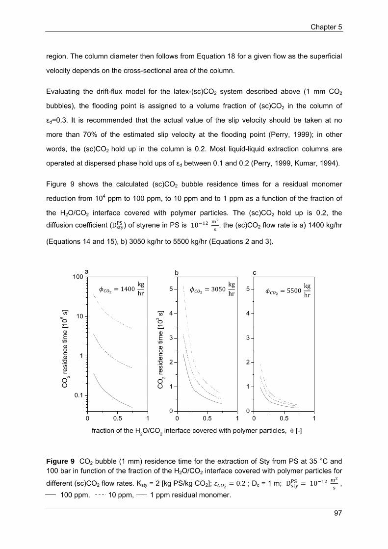
Chapter 5
97
3050kghr
1400kghr
5500kghr
region. The column diameter then follows from Equation 18 for a given flow as the superficial
velocity depends on the cross-sectional area of the column.
Evaluating the drift-flux model for the latex-(sc)CO2 system described above (1 mm CO2
bubbles), the flooding point is assigned to a volume fraction of (sc)CO2 in the column of
εd=0.3. It is recommended that the actual value of the slip velocity should be taken at no
more than 70% of the estimated slip velocity at the flooding point (Perry, 1999); in other
words, the (sc)CO2 hold up in the column is 0.2. Most liquid-liquid extraction columns are
operated at dispersed phase hold ups of εd between 0.1 and 0.2 (Perry, 1999, Kumar, 1994).
Figure 9 shows the calculated (sc)CO2 bubble residence times for a residual monomer
reduction from 104 ppm to 100 ppm, to 10 ppm and to 1 ppm as a function of the fraction of
the H2O/CO2 interface covered with polymer particles. The (sc)CO2 hold up is 0.2, the
diffusion coefficient (DstyPS ) of styrene in PS is 10 , the (sc)CO2 flow rate is a) 1400 kg/hr
(Equations 14 and 15), b) 3050 kg/hr to 5500 kg/hr (Equations 2 and 3).
Figure 9 CO2 bubble (1 mm) residence time for the extraction of Sty from PS at 35 °C and 100 bar in function of the fraction of the H2O/CO2 interface covered with polymer particles for
different (sc)CO2 flow rates. Ksty = 2 [kg PS/kg CO2]; 0.2 ; Dc = 1 m; D 10 ,
100 ppm, 10 ppm, 1 ppm residual monomer.
0 0.5 1
0.1
1
10
100
0 0.5 10
1
2
3
4
5
0 0.5 10
1
2
3
4
5
ba
CO
2 re
siden
ce ti
me [1
05 s]
c
CO
2 re
sidence
tim
e [1
03 s]
fraction of the H2O/CO
2 interface covered with polymer particles, [-]

Chapter 5
98
Figure 9 shows that the fraction of the H2O/CO2 interface covered with polymer particles
affects the residence time of the CO2 bubbles (and therefore also the column volume)
tremendously. Note that in Figure 9 the horizontal axis has a range of 0.1 < θ < 0.74. The
upper limit is θ = 0.74; the lower limit is arbitrarily chosen, according to the assumption
that mass transport of monomer from polymer particles into the (sc)CO2 phase is dominated
by the shuttle effect. How many particles actually adsorb to the H2O/CO2 interface depends
on the interfacial tensions between H2O(with surfactant)/polymer, polymer/CO2 and H2O(with
surfactant)/CO2 (Torza and Mason, 1970) and on the frequency the polymer particles arrive
at and move away from the H2O/CO2 interface. Predicting the number of particles adsorbed
at the H2O/CO2 interface according to the theory of Torza (1970), the upper limit value of
0.74 has been found.
As expected, increasing the (sc)CO2 flow rate, Figures 9a to 9c, decreases the monomer
concentration in the exiting (sc)CO2 flow, as well as the CO2 residence time in the column
(and therefore also the column volume). For the lowest (sc)CO2 flow rate, Figure 9a, the
actual column height is unrealistically high, i.e. 16 m for a residual monomer reduction from
104 ppm to 100 ppm to 1600 m for a reduction from 104 ppm to 1 ppm (at θ = 0.74). For a
flow rate of 3050 and 5500 kg (sc)CO2/hr, Figures 9b and 9c, acceptable column heights (< 4
m) have been calculated. Columns with an aspect ratio of about 3 are recommended, but
columns with an aspect ratio between 2 and 5 are also common (Seider, 2010). Based on
the aspect ratio in Figure 9b, (sc)CO2 flow rate of 3050 kg/hr, has been chosen as a base
case in this work.
Tables 1 and 2 give the CO2 bubble residence times in the column at some values of the
fraction of the H2O/CO2 interface covered with polymer particles, for a (sc)CO2 or dispersed
phase hold up of 0.2 and 0.1. The (sc)CO2 flow rate is 3050 kg/hr and the column diameter is
taken as 1 m. The 1 mm (sc)CO2 bubbles (specified by a sieve plate in the column) rise
through the column with a velocity of 1 mm/s (i.e. the slip velocity or hindered rising velocity
of the bubble swarm, calculated according to the drift flux approach, Equations 18 and 20).
As mentioned in the introduction, the diffusion coefficient (DstyPS ) of monomer in the polymer
phase increases from 10‐15m2
s to 10 < D < 10 due to the plasticizing effect of
CO2 (Alsoy, 1998). To analyze the effect of the transport constant of styrene in the polymer

Chapter 5
99
phase, the CO2 residence time has been calculated for D 10 and for D
10 .
Table 1 (sc)CO2 bubble residence time for operation with a CO2 hold up (εd) of 0.2 for a
residual monomer reduction from 104 ppm to 100 ppm, to 10 ppm and to 1 ppm as a function
of the fraction of the H2O/CO2 interface covered with polymer particles. *
D 10ms
D 10 ms
s s s s s s
0.74 314 491 697 196 295 403
0.3 785 1276 1698 442 707 982
*operating conditions: 100 bar, 35 °C, Ksty = 2 [kg PS/kg CO2], column diameter Dc = 1 m, 3050kg/hr, 1mm
Table 2 (sc)CO2 bubble residence time for operation with a CO2 hold up (εd) of 0.1 for a
residual monomer reduction from 104 ppm to 100 ppm, to 10 ppm and to 1 ppm as a function
of the fraction of the H2O/CO2 interface covered with polymer particles. *
D 10ms
D 10 ms
s s s s s s
0.74 589 982 1374 363 589 785
0.3 1571 2556 3436 982 1473 1963
*operating conditions: 100 bar, 35 °C, Ksty = 2 [kg PS/kg CO2], column diameter Dc = 1 m, 3050kg/hr, 1mm
For a (sc)CO2 hold up of 10%, a bubble residence time in the column more than twice the
time at a hold up of 20% is necessary to absorb the desired amount of monomer.
Consequently, the column height increases with approximately a factor 4, resulting in an
aspect ratio far above 5. Table 3 provides the calculated column heights corresponding to
the CO2 residence times reported in Tables 1 and 2. Only the column heights at the highest
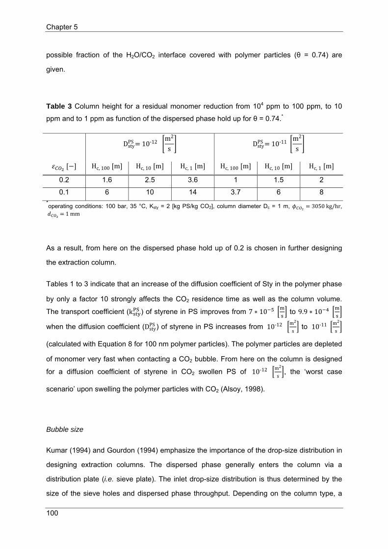
Chapter 5
100
possible fraction of the H2O/CO2 interface covered with polymer particles (θ = 0.74) are
given.
Table 3 Column height for a residual monomer reduction from 104 ppm to 100 ppm, to 10
ppm and to 1 ppm as function of the dispersed phase hold up for θ = 0.74.*
DstyPS 10‐12
m2
s Dsty
PS 10‐11m2
s
Hc,100 m Hc,10 m Hc,1 m Hc,100 m Hc,10 m Hc,1 m
0.2 1.6 2.5 3.6 1 1.5 2
0.1 6 10 14 3.7 6 8
*operating conditions: 100 bar, 35 °C, Ksty = 2 [kg PS/kg CO2], column diameter Dc = 1 m, 3050kg/hr, 1mm
As a result, from here on the dispersed phase hold up of 0.2 is chosen in further designing
the extraction column.
Tables 1 to 3 indicate that an increase of the diffusion coefficient of Sty in the polymer phase
by only a factor 10 strongly affects the CO2 residence time as well as the column volume.
The transport coefficient (k ) of styrene in PS improves from 7 ∗ 10 to 9.9 ∗ 10
when the diffusion coefficient (DstyPS ) of styrene in PS increases from 10‐12
m2
s to 10‐11
m2
s
(calculated with Equation 8 for 100 nm polymer particles). The polymer particles are depleted
of monomer very fast when contacting a CO2 bubble. From here on the column is designed
for a diffusion coefficient of styrene in CO2 swollen PS of 10‐12m2
s, the ‘worst case
scenario’ upon swelling the polymer particles with CO2 (Alsoy, 1998).
Bubble size
Kumar (1994) and Gourdon (1994) emphasize the importance of the drop-size distribution in
designing extraction columns. The dispersed phase generally enters the column via a
distribution plate (i.e. sieve plate). The inlet drop-size distribution is thus determined by the
size of the sieve holes and dispersed phase throughput. Depending on the column type, a

Chapter 5
101
steady drop-size distribution can be established, i.e. the drop-size distribution is practically
independent of the axial position in the column length. Therefore, an average drop size is
used to describe the extraction column. Kumar et al. (1996, 1994) give an overview of the
unified correlations for predicting drop or bubble sizes of several kinds of liquid-liquid
extraction columns. The predictions have been based upon experimental data obtained with
a well defined column diameter and column height. Korchinsky (1994) found that smaller
drops or bubbles require larger column diameters, because of a lower slip velocity relative to
the continuous phase. At the same time smaller drops provide larger specific interfacial
surface area, higher mass transfer rates and therefore columns become shorter. However, a
larger column diameter results in more axial dispersion in the column, hence decreasing
mass transfer (Godfrey, 1994). The axial mixing of the continuous phase is caused by the
tendency of the droplets to concentrate in the center of the column and move up together
with a core of continuous phase, which returns to the bottom through an annulus around the
wall, see Figure 10.
Figure 10 Schematic view of the axial mixing of the continuous phase in an extraction column induced by the dispersed phase.
In the present work, the average bubble size as well as the column diameter have been
defined, with respect to the flooding conditions according to the Wallis drift-flux model. From
these data the corresponding CO2 residence time and column height have been calculated.
Table 4 collects the CO2 residence time as well as the column height required for a residual
monomer reduction from 104 ppm to 100 ppm, to 10 ppm and to 1 ppm for 3 different
diameters of the CO2 bubbles.

Chapter 5
102
Table 4 CO2 residence time and the corresponding column height for a residual monomer
reduction from 104 ppm to 100 ppm, to 10 ppm and to 1 ppm in function of the CO2 bubble
diameter for θ = 0.74*
10‐3m s s s Hc,100 m Hc,10 m Hc,1 m
0.5 98 147 216 0.5 0.75 1.1
1 314 491 697 1.6 2.5 3.6
2 589 942 1306 3 4.8 6.7 *operating conditions: 100 bar, 35 °C, Ksty = 2 [kg PS/kg CO2], column diameter Dc = 1 m, 3050kg/hr,
DstyPS 10‐12 m2 s⁄ , 0.2
Increasing the bubble diameter results in higher CO2 residence times and larger columns,
similar to the findings of Korchinsky (1994), as mentioned above. The mass transfer
coefficient (k ) of styrene in the CO2 bubble decreases with increasing bubble size. Table
5 shows the required contact time of a CO2 bubble with a polymer particle for a developed
concentration profile in the CO2 bubble, calculated with Equation 10, as well as the mass
transfer coefficient (k ) of styrene in a CO2 bubble, calculated with Equation 11, with
respect to the contact time for 3 different bubble sizes.
Table 5 Contact time of a CO2 bubble with a polymer particle for a developed concentration profile in the CO2 bubble, calculated with Equation 10, and the corresponding mass transfer coefficient of styrene in the CO2 phase, calculated with Equation 11, as a function of the CO2 bubble size for θ = 0.74*
dCO2 10‐3m tcontact,CO2 [s] k 10
ms
0.5 2 10
1 7 5
2 29 2.5
*operating conditions: 100 bar, 35 °C, Ksty = 2 [kg PS/kg CO2], column diameter Dc = 1 m, 3050kg/hr,
DstyPS 10‐12 m2 s⁄ , 0.2
Large drops are internally well mixed, whereas small drops show an extra internal circulation
modifying the rigidity of the drop, i.e. the Marangoni effect, suppressing the benefit of a

Chapter 5
103
higher mass transfer rate in the dispersed phase (Bird, 2002). A bubble of 1 mm in diameter
with a slip velocity of ~ 1 mm/s is considered to be of realistic dimensions.
With respect to the mass balance over one stage, see Equation 2, extended over the total
height of the extraction column, the number of theoretical stages has been determined, see
Figure 2. It has been found that 12 equilibrium stages apply to reduce the residual monomer
in the latex from 104 ppm to 1 ppm. Knowing the number of stages required for the extraction
as well as the column height, the height equivalent of a theoretical stage follows from
Equation 26.
H N ∗ H (26)
Table 6 provides an overview of the operating conditions, design parameters and column
dimensions for the reduction of residual styrene in a PS latex from 104 ppm to 1 ppm by
extraction with scCO2.
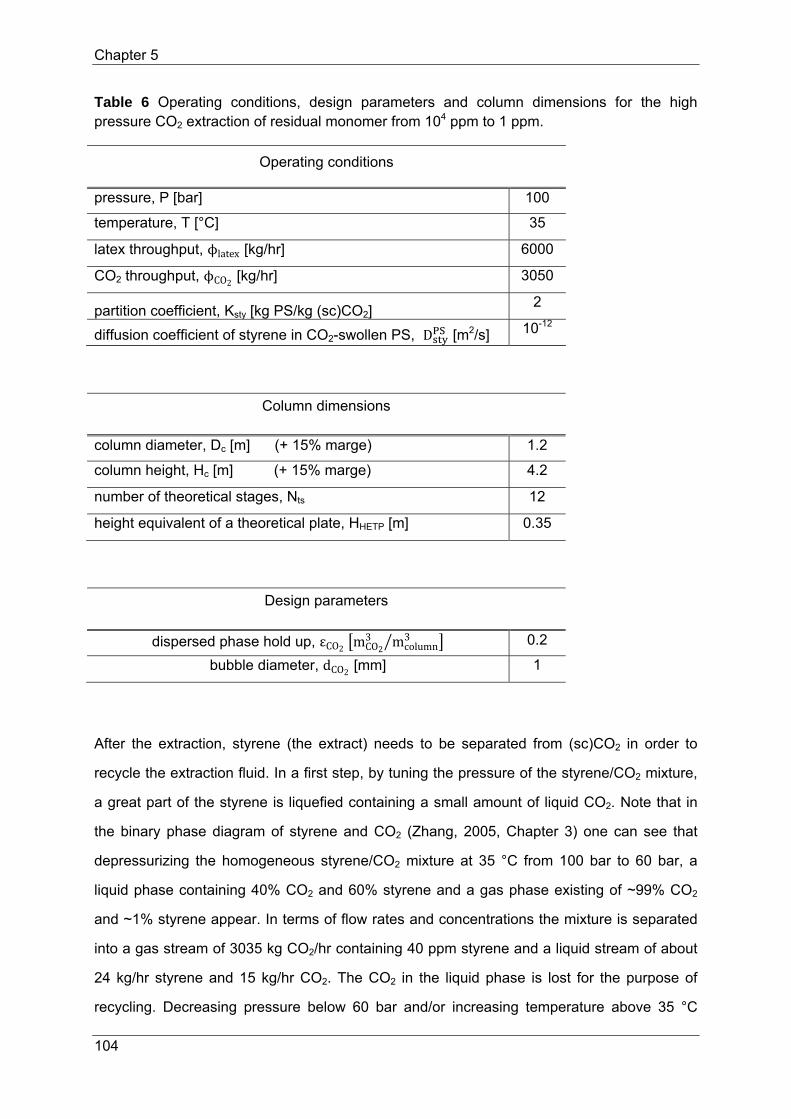
Chapter 5
104
Table 6 Operating conditions, design parameters and column dimensions for the high pressure CO2 extraction of residual monomer from 104 ppm to 1 ppm.
Operating conditions
pressure, P [bar] 100
temperature, T [°C] 35
latex throughput, ϕlatex [kg/hr] 6000
CO2 throughput, ϕCO2 [kg/hr] 3050
partition coefficient, Ksty [kg PS/kg (sc)CO2] 2
diffusion coefficient of styrene in CO2-swollen PS, D [m2/s] 10-12
Column dimensions
column diameter, Dc [m] (+ 15% marge) 1.2
column height, Hc [m] (+ 15% marge) 4.2
number of theoretical stages, Nts 12
height equivalent of a theoretical plate, HHETP [m] 0.35
Design parameters
dispersed phase hold up, εCO2 mCO23 mcolumn
3 0.2
bubble diameter, dCO2 [mm] 1
After the extraction, styrene (the extract) needs to be separated from (sc)CO2 in order to
recycle the extraction fluid. In a first step, by tuning the pressure of the styrene/CO2 mixture,
a great part of the styrene is liquefied containing a small amount of liquid CO2. Note that in
the binary phase diagram of styrene and CO2 (Zhang, 2005, Chapter 3) one can see that
depressurizing the homogeneous styrene/CO2 mixture at 35 °C from 100 bar to 60 bar, a
liquid phase containing 40% CO2 and 60% styrene and a gas phase existing of ~99% CO2
and ~1% styrene appear. In terms of flow rates and concentrations the mixture is separated
into a gas stream of 3035 kg CO2/hr containing 40 ppm styrene and a liquid stream of about
24 kg/hr styrene and 15 kg/hr CO2. The CO2 in the liquid phase is lost for the purpose of
recycling. Decreasing pressure below 60 bar and/or increasing temperature above 35 °C

Chapter 5
105
decreases the amount of liquid CO2 in the waste stream. The concentration of styrene in the
gaseous CO2 leaving the separator is very small but the CO2 still needs to be further purified
before recycling. The energy consumption and equipment costs to separate the styrene/CO2
mixture such that the liquid phase contains less CO2, are much higher than adding 15 kg new
CO2/hr to the recycle stream. So the operating conditions of the separation step are 35 °C
and 60 bar.3 It is suggested that in the top of separation vessel a demister is included to
prevent entrainment of liquid droplets.
In a second step the styrene (~40 ppm) is suggested to be removed from the gaseous CO2
flow by means of catalytic oxidation with oxygen (stoechiometric amount). The styrene/CO2
mixture is led over a fixed bed of Platinum (Pt) catalyst on a silica or alumina support in a
nitrogen-free environment. The styrene is completely converted into CO2 and H2O. The
oxidation is exothermic but requires some heat to start. The operating conditions in the
oxidation step have been chosen at 60 bar and 80 °C. The amount of catalyst needed has
been estimated at 180 kg when the Mcat/ϕstyrene O2 ratio is approximately 1 g/molhr-1 (for a
production capacity of 50 kt PS latex (45% solids)/yr). For more information concerning the
catalytic oxidation step the reader is referred to specialized literature (Seki, 2009, Evonik
Industries, 2011).
The purified latex or raffinate phase contains 1 ppm styrene but is still swollen with CO2 at a
pressure of 100 bar. Depressurizing the CO2-swollen latex is a key and delicate step as the
colloidal stability of the latex may change under pressure relief, i.e. foaming, coagulation,
etc.. These concerns are addressed in the next chapter.
Process flow diagram
Figure 11 shows the process flow diagram (PFD) for the reduction of the residual styrene
content in a PS latex from 104 ppm to 1 ppm by extraction with high pressure CO2. The
3 In the available binary phase diagrams of styrene-CO2 increasing the temperature to 75 °C (at 100 bar) (Suppes, 1989, Akgun, 2004) also creates a phase separation into a liquid phase containing 40 % CO2 but it appears that the mixture existing out of 98% CO2 is homogeneous at these conditions and phase separation will not occur. Accurate experimental data are necessary to verify this observation. When a phase separation of 40 % liquid and 99.5% gaseous CO2 can be achieved at 75 °C and 100 bar, the recompression of the CO2 recycle and therefore also the expensive compressor are no longer required. The overall cost and energy consumption decreases in comparison to the processes presented in the present section.

Chapter 5
106
respective streams entering and leaving the various pieces of equipment are indicated in
Figure 11a. The required work or power to heat or compress the streams are also given in
this figure, based on the information in Table 6.
Figure 11a Process flow diagram for the reduction of residual styrene in polystyrene latex from 104 ppm to 1 ppm by extraction with scCO2 at 100 bar and 35 °C. a) heat exchanger 1, b) pump, c) extraction column, d) heat exchanger 2, e) heat exchanger 3, f) pressure reducer, g) separator with demister, h) heat exchanger 4, i) catalytic oxidation, j) compressor. Green line represents latex circuit; black line represents CO2 circuit; red line represents the O2 stream.
Two separate circuits are distinguished in the PFD: one for latex and one for (sc)CO2. Latex
enters the circuit at 1 bar and 15 °C. As the extraction conditions are 100 bar and 35 °C, the
latex stream is heated (a) and pressurized (b). After extraction a purified latex product is
obtained.

Chapter 5
107
CO2 follows a more complicated circuit. After extraction of the latex, a styrene/CO2 mixture is
obtained, leaving the extraction column at 35 °C and 100 bar. As previously mentioned, the
separation step (g) requires a pressure decrease to 60 bar. In the Mollier diagram by Planck
and Kuprianoff, see Appendix C, one can see that isentropic depressurizing decreases the
temperature tremendously.4 Before separating the styrene from the CO2, the mixture needs
to be heated to 72 °C in order to allow the separator to operate at 35 °C and 60 bar. Before
entering the oxidation vessel (i) an isobaric temperature increase from 35 °C to 80 °C is
required. The purified CO2 at 60 bar and 80 °C is mixed with some fresh CO2 at 55 bar and
15 °C. The amount of fresh CO2 is less than 1% of the total CO2 required for extraction, so
there will be no significant influence on the temperature and pressure of the recycled CO2
stream. A compressor (j) isentropically pressurizes the CO2 to 100 bar, increasing the
temperature to 120 °C, see Mollier diagram, Appendix C. The energy flux of the CO2 stream
at 120 °C is very high, due to the relatively high heat capacity5 of dense CO2, and can be
used to heat the latex (a), the CO2 at the oxidation vessel (h) and partly the CO2 going to the
styrene/CO2 separator (d). Complementary heating the CO2 at the separator is achieved by
means of steam (e).
Figure 11b shows the complementary temperatures and pressures of the equipment in
Figure 11a.
4 As the amount of styrene in the styrene/CO2 mixture is so low, it has negligible influence on the behavior of CO2. 5 At 100 bar at 35 °C the specific heat of CO2 is 4.7 kJ/kg °C (deducted from the Mollier diagram, Appendix C).

Chapter 5
108
Figure 11b Temperature and pressure profiles corresponding with the PFD of the reduction of residual styrene in polystyrene latex from 104 ppm to 1 ppm by extraction with scCO2 at 100 bar and 35 °C shown in figure 7a. a) heat exchanger 1, b) pump, c) extraction column, d) heat exchanger 2, e) heat exchanger 3, f) pressure reducer, g) separator with demister, h) heat exchanger 4, i) catalytic oxidation, j) compressor. Green line represents the latex circuit; black line represents the CO2 circuit; red line represents the O2 stream.
Designing the (sc)CO2-based extraction process, calculations have been performed
assuming that the latex phase is swollen with (sc)CO2, so the molecular diffusion coefficient
of styrene in CO2-swollen PS (DstyPS ) is 10‐12
m2
s. It is therefore suggested that the start-up of
the extraction is performed semi-batch, i.e. (sc)CO2 is bubbled through the partially filled
column. Within a few cycles of the (sc)CO2 flow, the latex is swollen with CO2 and the actual
continuous extraction process is started. At this point also the required operating
temperatures and pressures of the equipment in every step are reached and the monomer
extraction by (sc)CO2 proceeds as described. Note that when the extraction column runs
stationary, some extra column volume is needed to allow for swelling of the latex phase. To
allow for a developed concentration profile in the polymer particles, i.e. Fo 0.1, the contact
time between the polymer particles and the (sc)CO2 (tcontact, p) is 1 s, calculated according to

Chapter 5
109
Equation 5 for 100 nm polymer particles and a diffusion coefficient (DCO2P ) of CO2 in PS of
10-15 m2/s.

Chapter 5
110
Equipment sizing and costs
Table 7 summarizes the costs, characteristic dimensions and process parameters for the
equipment as shown in Figure 11. The costs have been determined with the Aspen Process
Economic Analyzer based on a production capacity of 50 kt PS latex (45% solids)/year. All
equipment is made of stainless steel (316L) due to the corrosive properties of H2O/CO2
mixtures and the relatively high viscosity of the latex and the latex swollen with CO2.
Table 7 Characteristic dimensions and purchased costs of equipment
Capacity : 50 kt PS latex (45% solids)/yr
Extraction column Separator including demister Oxidation vessel
height [m] 4.2 1 1
diameter [m] 1.2 0.1 0.1
pressure [bar] 100 60 60
temperature [°C] 35 35 80
f.o.b. price* [k€] 614 45 45
material costs# [k€] 175 51 51
Compressor Pump
total power [kW] 31 20
f.o.b. price* [k€] 390 20
material costs# [k€] 40 12
Heat exchanger (a)
Heat exchanger (d)
Heat exchanger (e)
Heat exchanger (h)
duty [kW] 80.5 76.3 80.5 60.5
A [m2] 4.5 3.2 2.1 1.5
f.o.b. price* [k€] 39 34 18 22
material costs# [k€] 72 103 41 89 * f.o.b. price stands for free on board price, i.e. the price of the equipment without installation costs # the material costs include piping, instrumentation, insulation, etc.

Chapter 5
111
The total investment costs include materials for installation, i.e. piping, instrumentation,
insulation, etc., and labor costs. Table 8 generates the investment costs for the high
pressure CO2 extraction of residual monomer from 6000 kg PS latex (45% solids)/hr (≅ 50
kt/yr).
Table 8 Investment costs for the reduction of the residual monomer concentration in PS latex from 104 ppm to 1 ppm by extraction with (sc)CO2 at 100 bar and 35 °C for a production capacity of 50 kt PS latex (45% solids)/yr.
costs [M€]
Depreciation over 5 years Depreciation over 10 years [k€/yr] [€/ton latex] [k€/yr] [€/ton latex]
f.o.b. price* 1.2 material costs 0.7 labor costs 0.2
Total investment costs 2.1[M€] 417 [k€/yr] 8[€/ton latex] 208 [k€/yr] 4 [€/ton latex] * f.o.b. price stands for free on board price, i.e. the price of the equipment without installation costs
Table 9 collects the utility costs of the extraction process for a production capacity of 50 kt
PS latex (45% solids)/yr. The utility costs have been calculated based on price lists for steam
and electricity from DACE (2009), the CO2 price was delivered by Linde Gas Benelux, the
costs for the Pt/Al2O3 catalyst has been estimated based on a price list from Evonik (2011).
The costs for the O2 used in the oxidation step are not included due to the low consumption.
The start up costs for CO2 have been included.
Table 9 Utility costs for the reduction of the residual monomer concentration in PS latex from 104 ppm to 1 ppm by extraction with (sc)CO2 100 bar and 35 °C for a production capacity of 50 kt PS latex (45% solids)/yr. (see Figure 11a)
unit price amounts Costs [k€/yr] Costs [€/ton latex] electricity 0.14 €/kWh 51 kW 57.1 1.14 CO2
* 20 €/ton 3.05 ton/yr 61 ∗ 10 1∗ 10 15 ∗ 10 ton/hr 2.4 0.05
steam (1 bar, 100 °C)
30 €/ton 128 ∗ 10 ton/hr
31 0.61
catalyst 3500 €/kg 180 kg/yr 630 12.6
Total utility costs
720 14.4 * The CO2 amount used in the extraction process is based on a production capacity of 50 kt PS latex (45%
solids)/yr, without disruptions, i.e. cleaning of the equipment is performed once a year. In practice it is suggested the equipment is cleaned more often. The CO2 start up cost of 61 €/start up cycle then has to be included in the overall utility cost. Note, however, that the CO2 start up cost is negligible compared to the overall utility costs.

Chapter 5
112
In the first 5 years of the (sc)CO2 based extraction process reducing residual monomer level
in PS latex from 104 ppm to 1 ppm, the purification of the latex costs 22 €/ton latex. When the
investment costs are recovered, the cost of the extraction of the residual monomer from the
latex decreases to 14 €/ton latex.
Note that for a residual monomer reduction from 104 ppm to 100 ppm or to 10 ppm, the costs
for the purification of the latex are in the same range as for a reduction to 1 ppm. The higher
the allowed residual monomer concentration in the latex phase after extraction, the less CO2
required to perform the extraction, resulting in lower residence times needed, i.e. shorter
columns. The difference in CO2 needed to reduce the monomer concentration from 104 ppm
to 100 ppm, to 10 ppm or to 1 ppm, however, is small6, not affecting the total investment or
utility costs.
Steam stripping
Englund (1981) gives an overview of several types of latex strippers. The author reports
reducing the residual monomer level in latex with steam stripping is usually performed batch
wise, due to its simplicity and ease of operation. A batch of latex is charged into a simple
tank and steam is sparged through the latex at a certain flowrate, limited by foaming.
Defoaming agents are often used to suppress foaming (Kelley et al., 1978). Batch strippers
normally operate at 80-90% efficiency, but the amount of steam needed is higher than for
continuous countercurrent stripping. Englund (1981) states that for batch stripping the
frequency by which fresh steam bubbles contact the polymer particles is rate limiting. The
author refers to several patents for a description of a continuous countercurrent stripper.
Batch wise stripping as well as continuous countercurrent stripping for the reduction of
residual monomer level in PS latex from 104 ppm to 100 ppm are shortly discussed here.
6 The amount of CO2 required for residual monomer reduction in PS latex from 104 ppm to 100, 10 or 1 ppm, are 3000, 3022 and 3024 kg/hr, respectively. The value of the CO2 stream indicated in the present work is somewhat higher to account for the CO2 that dissolves in the H2O phase.

Chapter 5
113
Batch operation
The steam flow rate required for stripping a batch of 30 ton (45 % solids) PS latex in
approximately 5 hours (i.e. 6000 kg/hr) to reduce residual monomer from 104 ppm to about
100 ppm has been calculated according to Equation 27 (rs from B. Odedra, Synthomer, UK,
personal communication) .
ϕsteam Mdrysolids*rs (27)
rs stands for the steam mass flow rate per kg dry solids.
Assuming that stripping is performed at 90% efficiency, the required steam flow rate is 1700
kg/hr, calculated with Equation 27. In 5 hours a total amount of 8500 kg steam is needed to
reduce the residual monomer from 104 ppm to 100 ppm. The steam hold up in the latex is
usually about 10-20 % [m³ steam bubbles/m³ vessel) (Kantarci, 2005). The total liquid
volume in the stripping vessel at 20 % steam hold up becomes 38 m3. Englund (1981)
emphasizes that the batch stripping vessel is usually considerably larger than the liquid load
to allow for foaming. Assuming that the stripping vessel is enlarged by 50 % of the liquid
load, a tank of 57 m3 is needed. To operate the stripping vessel in the homogeneous bubble
flow regime, the superficial gas velocity needs to be smaller than 0.05 m/s (Kantarci, 2005).
The superficial gas velocity is defined as the ratio of the volumetric flow rate and the cross-
sectional area of the vessel. The density of steam at 100 °C is 0.6 kg/m3 (Perry, 1999). The
tank diameter for a superficial gas velocity of 0.05 m/s then is 2.2 m; the height of the vessel
is 14.5 m.
The latex batch, before stripping is started, is at 15 °C (i.e. latex from the polymerization
reaction is kept in a storage vessel). The steam at 100 °C is partly used for heating the latex,
i.e. 170 kg/hr or 850 kg steam during 5 hours of stripping (see Appendix D). So 10% of the
steam is used as heating source. As 10% is a significant part of the steam consumption, it is
added in the total steam flow required for stripping the latex.
Figure 12 illustrates the simple batch stripping vessel.

Chapter 5
114
Figure 12 Batch stripping vessel
The steam containing the residual monomer has been chosen to be purified in a water
treatment facility.
Continuously operated countercurrent stripping unit
Englund (1981) reports that the steam required to reduce residual monomer from 104 ppm to
100 ppm in a continuous countercurrent stripping vessel is less than the amount of steam
used in the batch stripping vessel. Assuming a throughput of 6000 kg PS latex/hr, the
number of theoretical stages is determined with the stage-to-stage calculation according to
Equation 2. Note that the monomer partition coefficient (Kmon) for the distribution of styrene
between the polymer particles and the steam decreases with decreasing residual monomer
concentration in the polymer particles, i.e. Kmon ↓ when Nts ↑, where Nts stands for the number
of theoretical stages. Table 10 shows the relation between the steam flow rate and the
number of equilibrium stages.
Table 10 Required number of theoretical stages in function of the steam flow rate for a residual monomer reduction from 104 ppm to 100 ppm.
steam flow rate kg
hr number of theoretical stages, Nts [-]
1700 13
1500 17
1400 23
1300 44

Chapter 5
115
Decreasing the steam flow rate increases the number of equilibrium stages needed to obtain
the same reduction in residual monomer. A further decrease in steam flow rate results in
unrealistic numbers of stages and is therefore not shown. Estimating the height equivalent to
one theoretical stage to be 35 cm – the same value as has been found in the CO2 extraction
process – the stripping vessel is 15.4 m high for a steam flow rate of 1300 kg/hr. For a
superficial gas velocity of 0.05 m/s (Kantarci, 2005) the column diameter has been calculated
to be 2.2 m.
Figure 12a shows the process flow diagram (PFD) for reduction of residual styrene by
continuous countercurrent stripping with steam.
Figure 12a Process flow diagram (PFD) for reduction of residual styrene from 104 ppm to ~ 100 ppm by continuous countercurrent stripping with steam. a) pump, b) heat exchanger, c) stripper.
In the PFD a pump is included to pressurize the latex from 1 to 1.3 bar, to overcome the
pressure drop inside the stripper. The latex flow is heated to the temperature of the stripping
vessel, i.e. 100 °C by the steam flow entering the column for stripping the latex. Therefore
somewhat more steam is required, i.e. 655 kg steam/hr for heating the latex (see Appendix

Chapter 5
116
D). Figure 12b shows the complementary pressures and temperatures corresponding to the
PFD, Figure 12a.
Figure 12b Temperature and pressure profiles for reduction of residual styrene from 104 ppm to about 100 ppm by continuous countercurrent stripping with steam corresponding to the PFD shown in figure 12a. a) pump, b) heat exchanger, c) stripper.
Similar to batch steam stripping the steam containing styrene is led to a water treatment
facility.
In the stripping vessels discussed above the residual monomer level in the latex was
reduced from 104 ppm to 100 ppm. For some latex products a reduction to 60 ppm residual
monomer is possible (Araújo et al., 2002). Reduction to lower levels of residual monomer is
hardly possible mainly due to thermodynamic (and to some extent transport) limitations. The
monomer activity coefficient in the polymer particles and as a consequence the equilibrium
monomer vapor pressure are very low at high conversions (X > 99%). Consequently,
monomer partitioning between the polymer phase and the steam phase is very low towards
the vapor phase, see Equation 28.
y ∗ P γ ∗ x ∗ P (28)

Chapter 5
117
In contrast to the CO2 extraction process, where the polymer phase is swollen with scCO2
increasing the monomer activity coefficient in the polymer phase, the partition coefficient for
steam stripping decreases with decreasing volume of the total amount of low molecular
weight species in the polymer phase see Chapter 1, Figure 1. At low monomer volume
fraction there is hardly any driving force for monomer anymore to diffuse to the vapor phase.
Moreover, the molecular diffusion coefficient of monomer in the polymer phase is very low
DmP 10‐15m2
s, i.e. a high mass transfer resistance in the particle phase.
Table 11 shows steam flow rates as a function of the number of equilibrium stages for a
monomer reduction from 104 to 10 ppm not taking into account the thermodynamic as well as
the transport limitation discussed above.
Table 11 Required number of theoretical stages in function of the steam flow rate for a residual monomer reduction from 104 to 10 ppm.
steam flow rate kg
hr number of theoretical stages, Nts [-]
15000 13
12000 20
11000 45
Equipment sizing and evaluation
Table 12 summarizes the characteristic dimensions, process parameters and costs for the
continuous steam stripping of residual monomer from PS latex, reducing the monomer level
from 104 ppm to about 100 ppm. The costs have been determined with Aspen Process
Economic Analyzer based on a production capacity of 50 kt PS latex (45% solids)/yr.
Stainless steel (316L) has been chosen as construction material.

Chapter 5
118
Table 12 Characteristic dimensions and purchased costs of equipment
column
heat exchanger
pump
height [m] 15.4 duty [kW] 411 total power [kW] 0.06 diameter [m] 2.2 A [m2] 4.8 f.o.b. price* [k€] 17
pressure [bar] 1
f.o.b.price* [k€] 10 material costs#
[k€] 11
temperature [°C] 100 material costs#
[k€] 41
f.o.b.price* [k€] 423 material costs# [k€]
177
* f.o.b. price stands for free on board price, i.e. the price of the equipment without installation costs # the material costs include piping, instrumentation, insulation, etc.
The total investment costs include materials for installation, i.e. piping, instrumentation,
insulation, etc., as well as labor costs. Table 13 gives the investment costs for the reduction
of residual monomer from 104 ppm to about 100 ppm with continuous steam stripping of
6000 kg PS latex/hr.
Table 13 Investment costs for the reduction of the residual monomer concentration in PS latex from 104 ppm to 100 ppm with 100 °C steam for a production capacity of 50 kt PS latex (45% solids)/yr.
costs [k€]
Depreciation over 5 years Depreciation over 10 years [k€/yr] [€/ton latex] [k€/yr] [€/ton latex]
f.o.b. price* 450 material costs 229 labor costs 96
Total investment costs 775 [k€] 155 [k€/yr] 3[€/ton latex] 77.5 [k€/yr] 2 [€/ton latex] * f.o.b. price stands for free on board price, i.e. the price of the equipment without installation costs
Table 14 collects the utility costs of the steam strip process for a production capacity of 50 kt
PS latex (45% solids)/yr. The utility costs have been calculated based on price lists for steam
and electricity from DACE (2009).

Chapter 5
119
Table 14 Utility costs for the reduction of the residual monomer concentration in PS latex from 104 ppm to 100 ppm with 100 °C steam for a production capacity of 50 kt PS latex (45% solids)/yr.
unit price amount Costs [k€/yr] Costs [€/ton latex] electricity 14 ct/kWh 0.061 kW 0.07 0.001 steam 30 €/ton 1.96 ton/hr 469 9.38
Total utility costs
718.9 9.39
In the first 5 years of the steam stripping process reducing residual monomer level in PS
latex (45% solids) from 104 ppm to 100 ppm, the cost of purifying the latex by stripping the
residual monomer content with steam is 12 €/ton latex. When the investment costs are
recovered, the cost of the stripping process decreases to 9 €/ton latex.
Note that when a residual monomer reduction from 104 to 10 ppm would be thermodymically
possible (within time limits), the utility costs of the steam consumption will tremendously
increase as compared to the costs for a monomer reduction from 104 to 100 ppm.. For a
steam flow rate of 15000 kg steam/hr, the utility costs for steam are 75 €/ton latex.
Extraction of residual monomer with (sc)CO2 extraction in comparison to steam
stripping
The purification costs per ton latex for the steam stripping process and the (sc)CO2-based
extraction process to reduce residual monomer in PS latex from 104 ppm to 100 ppm for a
production capacity of 50 kt PS latex (45% solids)/yr, are respectively 12 and 22 €/ton latex
in the period the investment costs are recovered. After a depreciation time of 5 years, the
price for steam stripping is 9 €/ton latex, whereas the cost for the (sc)CO2 based extraction
process is 14 €/ton latex. The (sc)CO2-based extraction process reduces the residual
monomer level to 1 ppm for the same price as a reduction to 100 ppm or to 10 ppm. Steam
stripping, however, reduces the residual monomer level in the latex to only about 100 ppm or
somewhat lower, but certainly not to a level of 1 ppm.

Chapter 5
120
Concluding remarks
Extraction with CO2 to reduce residual monomer from 104 ppm to 1 ppm in a countercurrent
extraction process in a column has been designed. Latex has been chosen as the
continuous phase in which 1 mm CO2 bubbles are dispersed with a hold up of 20 %. The
column is operated at 100 bar and 35 °C. The partition coefficient of monomer between the
CO2-swollen polymer particles and the CO2 phase is a key parameter in the performance of
the liquid-liquid extraction column in terms of the degree of residual monomer reduction. Due
to the plasticizing effect of (sc)CO2 the time constant for mass transport of monomer inside
the polymer particles decreases tremendously compared to non swollen polymer particles.
The mass transport mechanism is governed by the shuttle effect, due to the Brownian motion
of the polymer particles from and to the H2O/CO2 interface. A column volume of 4.75 m3
applies for a throughput of 6000 kg PS latex (45% solids)/hr.
The extraction process reducing the residual monomer costs 22 €/ton latex for a production
capacity of 50 kt PS latex (45% solids)/yr (for a reduction from 104 to 100 ppm, to 10 ppm or
to 1 ppm). Continuous steam stripping to reduce the residual monomer level in the latex from
104 ppm to 100 ppm only costs 12 €/ton latex. The lowest residual monomer concentration in
latex of 1 ppm can certainly only be achieved by extraction with (sc)CO2.

Chapter 5
121
References
M. Akgün, D. Emel, N. Baran, N. A. Akgün, S. Deniz, S. Dinçer, “Styrene-carbon dioxide phase equilibria at high pressures”, J. Supercritical Fluids, 2004, 31, 27-32
H. E. A. van den Akker, “Liquid-liquid spray columns – Hydrodynamic stability and reduction of axial mixing”, PhD Thesis, 1978, Eindhoven University of Technology, The Netherlands
H. E. A. van den Akker, R. F. Mudde, E. Stammers, “Fysische transportverschijnselen: 200 vraagstukken”, 1997, 2nd ed., Delft University Press, The Netherlands
E. Alper, B. Wichtendahl, W.-D. Deckwer, “Gas absorption mechanism in catalytic slurry reactors”, Chem. Eng. Sci., 1980, 35, 217-222
S. Alsoy, J. L. Duda, “Supercritical devolatilization of polymers”, AIChE, 1998, 44, 3, 582-590
P. H. H. Araújo, C. Sayer, J. G. R. Poço, R. Guidici, “Techniques for reducing residual monomer content in polymers: A review”, Polym. Eng. Sci., 2002, 42, 7
A. A. C. M. Beenackers, W. P. M. Van Swaaij, “Mass transfer in gas-liquid slurry reactors, a review article”, Chem. Eng. Sci. , 1993, 48, 18, 3109-3139
R. B. Bird, W. E. Stewart, E. N. Lightfoot, “Transport phenomena”,2002, 2nd edition, J. Wiley and sons Inc., New York
D. W. Brilman, W. P. M. van Swaaij, G. F. Versteeg, “A one-dimensional instationary heterogeneous mass transfer model for gas absorption in multiphase systems”, Chem. Eng. and Process., 1998, 37, 471-488
C. H. Chon, K. D. Kihm, “Empirical correlation finding the role of temperature and particle size for nanofluid (Al2O3) thermal conductivity enhancement”, Appl. Phys. Lett., 2005, 87, 153107, 1-3
A. B. De Haan, H. Bosch, “Fundamentals of industrial separations”, 2007, 2nd edition, The Netherlands
Dutch Association of Cost Engineers (DACE), “Prijzenboekje”, 27th ed., 2009
E. Dumont, H. Delmas, “Mass transfer enhancement of gas absorption in oil-in-water systems: a review”, Chem. Eng. and Process., 2003, 42, 419-438
S. M. Englund, “Monomer removal from latex”, Chem. Eng. Progr., 1981, 55-59; and references therein
J. van Deuren, T. Lloyd, S. Chhetry, R. Liou, J. Peck, Federal Remediation Technologies Roundtable, “Remediation technologies screening matrix and reference guide”, 4th ed., 2002, Washington
R. G. Gilbert, “Emulsion polymerization, A mechanistis approach”, Academic Press, 1995
J. C. Godfrey, M. J. Slater (Eds.), “Liquid-liquid extraction equipment”, 1994, J. Wiley and sons Inc., New York
C. Gourdon, G. Casamatta, G. Muratet, “Population balance based modeling of solvent extraction columns” in “Liquid-liquid extraction equipment”, eds. J. C. Godfrey, M. J. Slater, 1994, J. Wiley and sons Inc., New York

Chapter 5
122
S. J. Jang, “Role of Brownian motion in the enhanced thermal conductivity of nanofluids”, Appl. Phys. Lett., 2004, 84, 21, 4316
C. Joly-Vuillemin, C. Bellefon, “Solids effects on gas-liquid, Chem. Eng. Sci., 1999, 51, 10, 2149-2158
N. Kantarci, F. Borak, K. O. Ulgen, “Review: Bubble column reactors”, Proc. Biochem., 2005, 40, 2263-2283
E. L. Kelley, R. W. Harrison, B. B. Harris, “Defoamers: their theory and application with regard to the paint industry”, Polym., Paint and Colour J., 1978, 168, 734
M.F. Kemmere, M. Cleven, M. A. van Schilt, J. T. F. Keurentjes, “Process design for the removal of residual monomer from latex products using supercritical carbon dioxide”, Chem. Eng. Sci., 2002, 57, 3929-3937
A. Kumar, S. Hartland, “Empirical prediction of operating variables” in “Liquid-liquid extraction equipment” , eds. J. C. Godfrey, M. J. Slater, 1994, J. Wiley and sons Inc., New York
A. Kumar, S. Hartland, “Unified correlations for the prediction of drop size in liquid-liquid extraction columns”, Ind. Eng. Chem. Res., 1996, 35, 2682-2695
W. L. McCabe, J. C. Smith, P. Harriott, “Unit operations of chemical engineering”, 2001, 6th edition, McGraww-Hill, New York
J. H. Perry, Chapter 15, “Liquid-liquid extraction equipment” in “Chemical Engineer’s Handbook”, 1999, McGraw-Hill, New York
J. F. Richardson, W. N. Zaki, “Sedimentation and fluidization: part 1”, Trans. Inst. Chem. Eng., 1954, 32, 35
C. A. Scholtens, J. Meuldijk, A. A. H. Drinkenburg, “Production of copolymers with a predefined intermolecular chemical composition distribution by emulsion polymerisation in a continuously operated reactor”, Chem. Eng. Sci., 2001, 56, 955
W. D. Seider, J. D. Seader, D. R. Lewin, Widagdo, “Product and process design principles – Synthesis, analysis and evaluation”, 3th ed., 2010, John Wiley and sons Inc., USA
T. Seki, B. Alfons, “Catalytic oxidations in dense carbon dioxide”, Chem. Rev., 2009, 109, 6, 2409-2454
M. J. Slater, “Rate coefficients in liquid-liquid extraction systems”, in “Liquid-liquid extraction equipment”, eds. J. C. Godfrey, M. J. Slater, 1994, J. Wiley and sons Inc. , New York
G. J. Suppes, M. McHugh, “Phase behavior of the carbon dioxide-styrene system”, J. Chem. Eng. Dat., 1989, 34, 310-312
S. Torza, S. G. Mason, “Three-phase interactions in shear and electrical fields”, J. Colloid Interface Sci., 1970, 33, 1, 67-83
H. Vinke, P. J. Hamersma, J. M. H. Fortuin, “Enhancement of the gas-absorption rate in agitated slurry reactors by gas-absorbing particles adhering to gas bubbles”, Chem. Eng. Sci., 1993, 48, 12, 2197-2210
G. B. Wallis, “One-dimensional two-phase flow”, 1969, McGraww-Hill, New York
J. Welty, C. E. Wicks, R. E. Wilson, “Fundamentals of momentum, heat, and mass transfer”, 2001, 4th ed., Wiley, Chichester

Chapter 5
123
J. A. Wesselingh, “The velocity of particles, drops and bubbles”,Chem. Eng. Process., 1987, 21, 9-14
M. Xu, J. A. Finch, A. Uribe-Salas, “Maximum gas and bubble surface rates in flotation columns”, Inter. J. Miner. Process., 1991, 32, (3/4), 233
S. X. Zhang, W. H. Ray, “Modeling and experimental studies of aqueous suspension polymerization processes. 3. Mass transfer and monomer solubility effects”, Ind. Eng. Chem. Res., 1997, 36, 1310-1321
J. Zhang, L. Gao, X. Zhang, B. Zong, T. Jiang, B. Han, “Phase behaviors, density, and isothermal compressibility of styrene + CO2, ethylbenzene + CO2, and ethylbenzene + styrene+ CO2 systems”, J. Chem. Eng. Data, 2005, 50, 1818-1822

Chapter 5
124
Appendix A
According to Newton’s second law, three forces act on a (free falling) rigid sphere moving
through a liquid (stationary momentum balance) (De Haan, 2007, McCabe, 2001):
0 = external force – buoyant force – drag force
0 F F F (A.1)
The external force is in this case the gravitational force, the buoyant force is a force acting
parallel with the external force but in opposite direction, and the drag force appears
whenever there is relative motion between the spheres and the liquid.
F F m ∗ g V ∗ ρ ∗ g ∗
∗ ρ ρ ∗ g
(A.2)
The drag force is caused by the shear stresses at the surface of a particle moving through a
viscous liquid as well as in eddies in a possible wake and is generally described with a drag
coefficient, Equation A.3.
F C ∗ A ∗ ∗ ρ ∗ v C ∗ ∗
∗ ∗ ρ ∗ v (A.3)
The force balance, Equation A.1, then becomes
0 ∗
∗ ρ ρ ∗ g C ∗ ∗
∗ ∗ ρ ∗ v (A.4)
The terminal settling velocity is defined in Equation A.5:
v ∗ ∗ ∗
∗ ∗ (A.5)
For low Reynolds numbers, (i. e.Re v∞*ddispersedphase*ρcontinuousphase
μ < 1, creep flow) the drag
coefficient for rigid spheres is C (Bird et al., 2002).
The terminal rising (i.e. = settling velocity) velocity of a CO2 bubble then becomes:
v ∗ . ∗
(A.6)
Table A.1 gives the physical constants of the dispersed CO2 phase as well as of the
continuous latex phase used to calculate the terminal rising velocity (v∞) of a CO2 bubble.

Chapter 5
125
Table A.1 Physical constants of CO2 as well as of PS latex used to calculate the terminal rising velocity of a CO2 bubble through the latex.
ρCO2bubble (35 °C, 100 bar) 720 kg/m³ ρlatex 1020 kg/m³ dCO2bubble 10-3 m μlatex 64 mPas
The terminal rising velocity becomes:
v∞ = 3 ∗ 10 (A.7)
Note that the Reynolds number is indeed < 1, see Equation A.8.
Re ∗ ∗
∗ ∗ ∗
∗≅ 0.05 (A.8)
The rising velocity of the bubble swarm in the column according to Equation A.9 is:
v v ∗ 1 ε (A.9)
where n depends on Re, see Equations 21-24, and has a value of 4.65 fo the Reynolds
number of 0.05, see Equation A.8. For a CO2 hold up of 20% [m³ CO2 bubbles/m³ column] in
the column, vs becomes:
vs 3*10‐3* 1‐0.24.65‐1
≅1*10‐3m
s (A.10)

Chapter 5
126
Appendix B
In this appendix the process flow diagram (PFD), Figures 11a and 11b, is explained into
detail. The annotation used in this section corresponds to that in the respective figures.
1. Extraction column (c)
The extractor, 1.2 m in diameter and 4.2 m high, is operated at 100 bar and 35 °C. The
overall heat balance over the extraction column is expressed in Equation B.1:
ϕq column ϕm,CO2*Cp,CO2*∆T ϕm,latex*Cp,latex*∆T ϕq (B.1)
where ϕm,i, Cp,i and ϕq stand for the mass flow rate of phase i, for the specific heat of phase
i and for the heat flow lost to the surroundings. To prevent temperature gradients inside the
column due to cooling by the surrounding air, it is insulated with e.g. mineral wool. The air
temperature is assumed to be 15 °C. The heat flow rate from the extraction column to the
surroundings follows from Equation B.2. Note that the resistances against heat transfer from
the liquid in the column to the wall of the column as well as from the wall to the surrounding
air have been neglected.
ϕq U*A*∆T (B.2)
where U and A stand for the overall heat transfer coefficient and the column area
respectively. Mineral wool has a thermal conductivity coefficient ( ) of 0.0523W
m (Perry,
1999). An estimation of the overall heat transfer coefficient for mineral wool follows from
Equation B.3,
U λ
δinsulation
W
m2 1
W
m2 for an insulation thickness of 5 cm (B.3)
The resulting heat flow rate from the liquid in the column to the surrounding air then
becomes:
ϕ 1 ∗∗ . ∗ .
∗ 35 15 kW ≅ 0.32 kW (B.4)
Table B.1 gives the physical constants of latex as well as of CO2 at 100 bar at 35 °C.

Chapter 5
127
Table B.1 Flow rates and physical constants of latex as well as of CO2 at 100 bar at 35 °C
ϕ ρ Cp
kg/hr kg/s kg/m³ kJ/kg °C latex 6000 1.67 1020 2.9 CO2 3050 0.85 720 4.7
As the mass flow rate as well as the specific heat7 inside the column is known, the
temperature loss to the environment easily follows from Equation B.5:
∆T ϕq
ϕCO2 latex*Cp,CO2 latex
0.32
2.52*3.5 ≅0.04 (B.5)
So heat loss from the extraction unit to the environment is negligible.
2. Pump (b)
6000 kg PS latex/hr is delivered at 15 °C at 1 bar. Before entering the extraction column the
latex has to be pressurized to 100 bar and heated to 35 °C. For pressurizing the latex from 1
bar to 100 bar, a plunger pump has been chosen. The shaft work required for pressurizing
the latex has been calculated with Equation B.6:
ϕ , pump ϕ , ∗
(B.6)
where ϕ , and ρ stand for the mass flow and density of latex, see Table B.1. The
shaft work of the pump then becomes:
ϕ , pump 1.67 ∗ ∗ 10 W 16.2 kW (B.7)
Pressurizing heated latex increases the chance on fouling inside the pump. Regularly
cleaning has to be taken into account.
It is assumed the pump works at 80% of its efficiency, so
ϕw,tot pump ϕw,shaft pump
.≅20.3kW (B.8)
7 Inside the extraction column the total mass flow rate is 9050 kg/hr (= 2.52 kg/s) being 34 % CO2, with a specific heat of 4.7 [kJ/kg °C] (deducted from Mollier diagram) and 66 % latex, with a specific heat of 2.9 [kJ/kg °C] (Perry, 1999). Then the specific heat of the CO2/latex mixture is 3.5 [kJ/kg °C].

Chapter 5
128
20% of the work the pump delivers is dissipated in heat. Assuming that all the heat
dissipated is transferred to the latex, a temperature rise of the latex follows from Equation
B.9.
∆T . ∗ϕw,tot pump
, ∗ ,≅ 0.8 (B.9)
The latex still has to be heated by 19.2 °C, see heat exchanger (a).
3. Compressor (j)
The energy balance for the adiabatically operating compressor is expressed in Equation
B.10.
ϕw,shaft compressor ϕm,CO2*∆ u P
ρ ϕm,CO2*∆h (B.10)
3050 kg CO2/hr enters the compressor at 80 °C and 60 bar. The extraction conditions have
been chosen at 35 °C and 100 bar, so CO2 needs to be compressed and cooled. According
to the Mollier diagram, Appendix C, isentropic compression (i.e. s = 1.25 kcal/°C) from 60 to
100 bar requires 29.3 kJ/kg (i.e. 7 kcal/kg).
ϕw,shaft compressor 0.85*29.3 kW ≅25 kW (B.11)
At 80 % efficiency, the total power the compressor needs is
ϕw,tot compressor . kW ≅31 kW (B.12)
At the same time due to the isentropic compression the temperature of the CO2 rises to 120
°C. Isobaric cooling of the CO2 flow from 120 °C to 35 °C, generates 256 kJ/kg (i.e. 61
kcal/kg), which can be used to heat the latex and CO2 flow at other stages in the process,
see PFD, Figure 11, heat exchanger a, d and h.
4. Separation vessel (g)
To separate (to some extent) styrene from the CO2 leaving the extraction column, operating
conditions of the separation vessel have been chosen at 35 °C and 60 bar. The gas flow

Chapter 5
129
superficial velocity (vs) has been taken at 0.5 m/s. Table B.2 gives the physical constants
used in the calculation of the required vessel surface area.
Table B.2 Flow rates and physical constants used for the calculation of the vessel area perpendicular to flow at 35 °C at 60 bar.
ϕ , 3074 kg/hr 0.85 kg/s ρCO2 300 kg/m³ vs 0.5 m/s
The vessel area perpendicular to flow (Aseparator, ) has been calculated with Equation B.13.
Aseparator, ϕv,CO2 stryrene
vs (B.13)
where ϕv,CO2 stryrene stands for the volume flow of the mixture CO2/styrene.
Aseparator 0.85
300*
1
0.5 m2 ≅60 cm2 (B.14)
Including a demister, the dimensions of the separation vessel have been estimated at 0.1 m
in diameter and 1 m in height.
5. Oxidation vessel
In a second separation step the styrene (~40 ppm on weight base) is suggested to be
removed from the gaseous CO2 flow by means of catalytic oxidation with pure oxygen
(stoechiometric amount). The styrene/CO2 mixture is led over a fixed bed of Platinum (Pt)
catalyst on a silica or alumina support in a nitrogen free environment. The styrene is
completely converted into CO2 and H2O. The oxidation is exothermic but requires some heat
to start. The operating conditions in the oxidation step have been chosen at 60 bar and 80
°C. The amount of catalyst needed has been estimated at 180 kg when the Mcat/ϕstyrene O2
ratio is approximately 1 g/molhr-1 (for a production capacity of 50 kt PS latex (45% solids)/yr).
For more information concerning the catalytic oxidation step the reader is referred to
specialized literature (Seki, 2009, Evonik Industries, 2011).
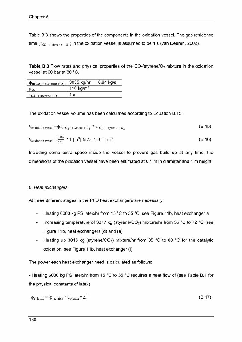
Chapter 5
130
Table B.3 shows the properties of the components in the oxidation vessel. The gas residence
time (τCO2 styrene O2) in the oxidation vessel is assumed to be 1 s (van Deuren, 2002).
Table B.3 Flow rates and physical properties of the CO2/styrene/O2 mixture in the oxidation vessel at 60 bar at 80 °C.
ϕ , 3035 kg/hr 0.84 kg/s ρCO2 110 kg/m³ τCO2 styrene O2 1 s
The oxidation vessel volume has been calculated according to Equation B.15.
Voxidationvessel ϕV,CO2 styrene O2*τCO2 styrene O2 (B.15)
Voxidationvessel0.84
110*1 m³ ≅7.6*10‐3 m3 (B.16)
Including some extra space inside the vessel to prevent gas build up at any time, the
dimensions of the oxidation vessel have been estimated at 0.1 m in diameter and 1 m height.
6. Heat exchangers
At three different stages in the PFD heat exchangers are necessary:
- Heating 6000 kg PS latex/hr from 15 °C to 35 °C, see Figure 11b, heat exchanger a
- Increasing temperature of 3077 kg (styrene/CO2) mixture/hr from 35 °C to 72 °C, see
Figure 11b, heat exchangers (d) and (e)
- Heating up 3045 kg (styrene/CO2) mixture/hr from 35 °C to 80 °C for the catalytic
oxidation, see Figure 11b, heat exchanger (i)
The power each heat exchanger need is calculated as follows:
- Heating 6000 kg PS latex/hr from 15 °C to 35 °C requires a heat flow of (see Table B.1 for
the physical constants of latex)
ϕq,latex ϕm,latex*Cp,latex*∆T (B.17)

Chapter 5
131
ϕq,latex 1.67*2.9*20 W ≅96.7kW (B.18)
Pressurizing the latex flow increases its temperature by 0.8 °C. Dimensioning the heat
exchanger, only 80.5 kW is required to increase the temperature from 15 °C to 34.2 °C.
- According to the Mollier diagram an isobaric temperature increase of the styrene/CO2
mixture (see Table B.2 for the physical constants) from 35 °C to 72 °C at 100 bar
corresponds to 176 kJ/kg (i.e. 42 kcal/kg).
ϕq,C separator ϕm,CO2*∆h (B.19)
ϕq,C separator 0.85*176 kW ≅150 kW (B.20)
- Increasing the temperature of the styrene/CO2 mixture (see Table B.3 for the physical
constants) from 35 °C to 80 °C at 60 bar requires 71 kJ/kg (i.e. 17 kcal/kg).
ϕq,C oxidationvessel 0.84*71 kW ≅60.5 kW (B.21)
As mentioned in the section 3, the CO2 after compression provides a latent heat loss of 256
kJ/kg (i.e. 61 kcal/kg) upon decreasing the temperature from 120 °C to 35 °C at 100 bar. In
the best scenario the CO2 latent heat loss is used to heat other streams in the following order
- At the catalytic oxidation (71 kJ/kg = 17 kcal/kg), heat exchanger (h)
The respective temperatures of the heated and cooled CO2 flow: 35 °C → 80 °C and
120 °C → 78 °C
- At the separator (~96.4 = 23 kcal/kg), heat exchanger (d)
The respective temperatures of the heated and cooled CO2 flow: 35 °C → 48 °C and
78 °C → 50 °C, heat exchanger (d)
- Before the pump pressurizing the latex flow ( ~ 88 kJ/kg = 21 kcal/kg), heat
exchanger (a)
The respective temperatures of the heated latex and cooled CO2 flow: 15 °C → 34.2
°C and 50 °C → 35 °C
At the separator one extra heat exchanger is required heating the CO2 flow from 48 °C to 72
°C. Steam at 100 °C and 1 bar is used for this purpose. The amount of steam required has

Chapter 5
132
been calculated dividing the required power by the heat of vaporization of steam (Perry,
1999) at 100 °C, Equation B.22.
ϕsteam ϕq,e heatexchangere
kg
hr80.5*3600
2257.8kg
hr128
kg
hr (B.22)
Dimensioning the different heat exchangers described above, has been performed according
to Equation B.23.
ϕq,i heatexchangeri U*A*∆Tln (B.23)
where ∆Tln stands for the logarithmic mean temperature difference between the heated and
cooled stream.
Table B.4 gives the physical properties as well as the resulting heat transfer area of the
different heat exchangers (h), at the oxidation vessel, (d) at the separator, (a) to heat the
latex, (e) at the separator.
Table B.4 Physical properties as well as the resulting heat transfer area for the heat exchangers (h), at the oxidation vessel, (d) at the separator, (a) to heat up the latex, (e) at the separator
heat exchanger i ϕq,i [kW] U W
m2 °C
8 ∆Tln [°C] Ai [m²]
h 60.5 1000 41.5 1.5
d 76.3 1000 24 3.2
a 80.5 1000 17.8 4.5
e 80.5 1000 38.8 2.1
7. Pressure reducer (f)
Before the styrene/CO2 mixture enters the separator, its pressure is expanded from 100 bar
to 60 bar. This process generates 21 kJ/kg (i.e. 5 kcal/kg) that is lost, see Equation B.24.
ϕq,C pressurereducer 0.85*21 kW ≅18 kW (B.24)
8 The overall heat transfer coefficient of CO2 is estimated at 1000
W
m2 °C, the same value as for H2O (Perry, 1999)
as the density of both components are very similar.

Chapter 5
133
Appendix C

Chapter 5
134
Appendix D
In a batch stripping vessel, steam at 100 °C is directly contacted with the cold latex of 15 °C.
The steam therefore condenses at 100 °C. The amount of steam needed to heat the latex
has been calculated with Equation D.1. Table D.1 shows the physical properties of latex.
Table D.1 Physical properties of latex
ϕ ρ Cp
kg/hr kg/s kg/m³ kJ/kg °C latex 6000 1.67 1020 2.9
ϕsteam ∗ , ∗ , (D.1)
ϕsteam 15*4.2*6000
2257.8kJhr
kJkg
170kg
hr (D.2)
In the continuous stripping process, the latex stream first needs to be heated before entering
the column. The amount of steam required to heat the latex from 15 °C to 100 °C, see
Equations D.3 to D.5.
ϕq, heatexchanger ϕm,latex*CP,latex*ΔT (D.3)
ϕq, heatexchanger 1.67*2.9*85≅411 kW (D.4)
ϕsteam ∗
.kJhr
kJkg
655kg
hr (D.5)


137
Chapter 6
High pressure carbon dioxide in the extraction of residual monomer
from latex products: additional results and outlook
Abstract
In retrospect to the previous chapters, this final chapter gives a perspective on some
challenges in the extraction of residual monomer from latex products with high pressure
carbon dioxide.
Monomer partitioning
The partition coefficient (Kmon) of the distribution of monomer between CO2-swollen polymer
and CO2 is the key issue in the extraction of residual monomer from latex with scCO2. The
phase behavior of a ternary system monomer-CO2-swollen polymer-CO2 is often estimated
by thermodynamic models based on the component properties. In Chapter 3 the large
deviation between the experimentally determined and the theoretically predicted partition
coefficient (Kmon) of the distribution of monomer between CO2-swollen polymer and CO2 has
been discussed. The polymers used in the present work have not been submitted to
annealing before experimental data have been collected. The polymer properties found in
literature as well as in the VLXE software (Laursen, 2003) databank, have been determined
from polymers which have been tempered at temperatures above their glass transition
temperature. The annealing process changes the polymer properties as it removes any
history effects as well as contaminants (van de Ven, 1975, Huvard et al., 1980). A proper
design of an extraction process for residual monomer reduction (and reduction of the level of
other low molecular weight species) from reactor products demands for partitioning data
based on the actual products formed during the polymerization. This will almost always mean

Chapter 6
138
that partition coefficients of residual monomer (and other relevant low molecular weight
species) have to be determined by experiments.
Colloidal stability
One of the challenges in the reduction of residual monomer in polymer (latex) products by
extraction with (sc)CO2 is the release of CO2 dissolved in the polymer particles. A rapid
pressure decrease leads to loss of colloidal stability, i.e. bubble formation and even foaming,
probably leading to surface coagulation/fouling. Foaming can be suppressed by introducing a
defoaming agent to the reactor product (Kelley et al., 1978). However, the characteristics of
the latex product can change, i.e. discoloration, hardness, etc.. Note that application of
defoaming agents adds contaminants to the latex product.
It has been observed experimentally1 that the first bottleneck in decreasing the pressure of a
scCO2 – latex mixture is the CO2 phase transition point, when CO2 changes from the
supercritical to the gas phase. The formation of gas bubbles in the latex may cause foaming
as a result of the presence of surface active species. Depending on the speed of the
pressure decrease, foaming is severe or moderate. Once the pressure is below the
supercritical pressure of 73 bar, decrease of the pressure can be controlled better than close
to the critical pressure. Decreasing the pressure from about 5 bar to atmospheric pressure is
also accompanied with some undesired phenomena. Note that particles are still swollen with
CO2 at these already low pressures. Release of CO2 is governed by mass transport. The
time constant for transport of CO2 out of the particles to the gas phase is probably larger than
the time constant for pressure decrease. So recording atmospheric pressure in the gas
phase ignores the CO2 present in the particles. Waiting for about 15 minutes allows CO2
transport from the particles to the gas phase, leading to a pressure increase. Repeating the
procedure of pressure decrease followed by CO2 gas release from the particles is
accompanied by fouling affixed to the wall of the vessel containing the latex. Also flocs of
polymer were observed. Note that about 15 minutes after a constant pressure of 1
atmosphere has been reached a coagulum free latex could be isolated. Industrial removal of
1 In the optical high pressure cell described in Chapter 3, latex was loaded with scCO2 at 100 bar at 35 °C. After 1 hour the pressure was relieved through a valve at the top of the high pressure cell.

Chapter 6
139
residual monomer with high pressure CO2 demands for filtration after complete pressure
release. Also cleaning of the equipment wall is necessary on a regular basis. The preliminary
observations make clear that an accurately controlled pressure decrease is a prerequisite for
a proper performance of a residual monomer reduction process based on (sc)CO2-based
extraction. Note that proper development of a pressure decrease procedure is also
applicable for e.g. emulsion vinylchloride/polyvinylchloride systems in emulsion and
suspension.
One of the alternative methods to allow for phase separation between the latex and the CO2
dissolved in the latex, is to chemically bind the CO2 by using a weak basic macroporous ion
exchange resin. CO2 reacts directly with primary or secondary amines generating their
respective carbamate salts (Riley et al., 1994), see Scheme 1 for the typical reversible
reaction.
Scheme 1. Reaction of amines with CO2.
The corresponding carbamate acid is not stable, only in the form of a sterically stabilized
anion. The CO2 dissolved in the latex can be captured by a proper amine when the latex/CO2
mixture is led over a macroporous weak basic ion exchanger containing amine groups. Saha
et al. (1999) as well as Samanta and Bandyopadhay (2009) discuss the kinetics as well as
the modeling of the absorption of CO2 into aqueous solutions of the sterically hindered amine
2-amino-2-methyl-1-propanol (AMP). Bonenfant et al. (2007) studied the CO2 absorption
capacities in aqueous 2-(2-aminoethylamino)ethanol (AEE) solutions. The authors mentioned
reported experimental observations of CO2 absorption in amine solutions from CO2
containing gas streams. The pressure in such processes are low to moderate, < 100 bar.
Nevertheless absorption of CO2 by leading the latex/CO2 mixture over an ion exchanger
containing amine groups is a promising method to remove the CO2 from the latex. Ion
Chapter 6
140
exchange resins saturated with CO2 by the reaction presented in Scheme 1 can be thermally
regenerated after washing out the latex particles with an amount of water as small as
possible. During the thermal regeneration the carbamate dissociates in CO2 and the amine
(note the analogy with the CO2 absorption process during the production synthesis gas for
ammonia synthesis).
Equilibrium between water and scCO2: pH-effects
Water in contact with carbon dioxide is known to become acidic due to the formation and
dissociation of carbonic acid, see Equation 1:
CO2 H2O⇌H2CO3⇌H HCO3‐ (1)
Organic species in an acidic medium can take up a proton, decreasing their solubility in CO2.
Thoews et al. (1995) measured the pH of water in contact with CO2 by observing UV-VIS
spectra of a pH indicator. The pH of water in equilibrium with scCO2 at equilibrium has been
found to be only slightly dependent of temperature in the range between 25 and 70 °C at
pressures ranging from 70 to 200 bar. Toews et al. (1995) reported a pH of water in
equilibrium with scCO2 between 2.8 and 3. Increasing pressure at constant temperature
decreases the pH. Increasing temperature at constant pressure increases the pH, due to the
lower solubility of CO2 in water at higher temperatures. The solubility behavior of CO2 in
water at supercritical conditions for CO2 resembles that of liquid CO2 in equilibrium with
water. The partial molar volume of liquid CO2 in water varies only slightly with pressure,
hence the solubility of liquid CO2 in water is rather independent of pressure. Li and Duan
(2007) report similar observations.
During the extraction of residual monomer from latex products with scCO2 the pH of the latex
will decrease with respect to the pH of the reactor product. The colloidal stability of the
latexes used in the experiments (vide supra), however, did not change. The latex used in the
experiments varied in pH from 5 to 9.

Chapter 6
141
Life Cycle Assessment
Green chemistry, low energy consumption, renewable resources, etc., are hot topics in
process technology. The ecological footprint of a product or process has never been so
emphasized as in the last two decades (Klöpffer, 2001-2006). Typically, a life cycle
assessment (LCA) is made to identify, quantify, interpret and evaluate the environmental
impact of a product or process. Van den Berg et al. (1995) defined LCA as a systematic
evaluation of the environmental impact of products or activities from the resources entering
the process to the ultimate waste disposal of the material. This so-called cradle-to-grave
concept implies the identification and quantification of emissions and material consumption
affecting the environment in all stages of the product life cycle. LCA is a diagnostic
engineering tool which can be used to compare existing or novel products or processes or
services with each other or with a standard.
Within LCA the definition of the system boundaries is very important. A functional unit
determines which products or processes can be meaningfully compared to each other. Note,
however, that in a comparative study, the compared products or processes are seldom
exactly identical. Van den Berg et al. (1995) described two solutions for this problem: define
a certain minimum level that all compared alternatives must obey, or leave qualitative
differences between compared alternatives out of the LCA calculations and describe them in
words. In either way, interpreting the LCA calculation results, one has to take into account
the assumptions made in the functional unit definition.
In every LCA it is necessary to define which environmental impacts have to be taken into
account. The International Organization for Standardization (ISO) published a series of
standards, including only headlines for impact categories: resource use, ecological
consequences and human health (ISO, 2007). In terms of more operational impact
categories, several areas have been indicated, e.g. toxicity potential (human and/or
ecotoxicity), energy consumption, global warming potential, acidification potential, land use,
etc (Van den Berg et al., 1995). In the next step, i.e. characterization, the contribution of
individual impacts per impact category has to be calculated. To perform this characterization
process objectively, the characterization results are normalized, i.e. the results are divided by
the actual or predicted magnitude for each impact category. Applying weighting factors, a

Chapter 6
142
single score or index for the total environmental impact of a product or process is obtained.
In the last stage of LCA, all previous stages and the assumptions made therein need to be
interpreted and evaluated. The robustness of the results needs to be tested, i.e. to check
whether conclusions hold even if critical and/or approximate data are changed. Such
evaluations typically cover sensitivity analysis, uncertainty analysis and data quality
assessment. Nevertheless, discussions on the methodology followed, and especially on the
choice of the functional unit, remains an important issue in the field of LCA.
Comparing the steam stripping process with the scCO2-based extraction process to reduce
residual monomer in latex products, the functional unit in an LCA can be assigned as the
residual monomer level in the latex. In this way the environmental impacts of each separation
process, i.e. steam stripping or extraction with scCO2, can be unambiguously compared. The
difficulty in interpreting the LCA results is hidden in the thermodynamic and transport
limitations of the steam stripping process to reduce the residual monomer level. The
monomer activity coefficient and as a consequence the monomer saturated vapor pressure
in the polymer phase, respectively in the surrounding vapor phase are very low at high
conversions (X > 99%). Consequently, monomer partitioning between the polymer phase and
the steam phase is very low towards the vapor phase, see Equation 2.
y ∗ P γ ∗ x ∗ P (2)
In contrast to the CO2 extraction process, where the polymer phase is swollen with (sc)CO2
increasing the monomer activity coefficient in the polymer phase with respect to the
unswollen polymer, the partition coefficient decreases with decreasing monomer mole
fraction in the polymer phase (ϕP), see Chapter 1, Figure 1. For low mole fractions of
monomer there is no driving force for monomer transfer to the vapor phase. Moreover, the
molecular diffusion coefficient of monomer in the polymer phase is very low
DmP 10‐15m2
s, i.e. there is high mass transfer resistance in the particle phase.
For some polymeric latexes a reduction to 60 parts per million (ppm) residual monomer has
been reported (Araújo et al., 2002). In the present work a final level of residual monomer in
the latex product of 100 ppm has been chosen as the lowest level of the residual monomer in
the latex with steam stripping. scCO2 as extraction medium is able to reduce the residual
monomer level in latex to 1 ppm with a slightly higher CO2 flow compared to a residual

Chapter 6
143
monomer reduction to 100 ppm. For a reduction of residual styrene in PS latex from 104 ppm
to 100 ppm 3000 kg scCO2/hr is needed with a concentration of 90 mol styrene/ m3 scCO2 in
the outgoing CO2 flow. Under the same circumstances, 3025 kg scCO2/hr is required to
reduce the residual styrene level in PS latex from 104 ppm to 1 ppm.
Applying a LCA to study the environmental impact of the scCO2 based extraction process
compared to the steam stripping to reduce residual monomer in latex delivers knowledge on
emission, energy consumption, etc.. However, the monomer reduction in latex with scCO2
extraction to only 1 ppm may counter balance the impact factors.
Concluding remarks
The work described in this thesis covers several important aspects of residual monomer
reduction in polymer products. High pressure or scCO2 has the potential to decrease time
constants for monomer transport in the polymer phase as well as to reach very low levels of
the residual monomer concentration in polymers (1 ppm) with a relatively small equipment
size. Performance compared with common techniques like steam stripping is better as the
final residual monomer level aimed at becomes lower.
Although the implementation of high pressure or scCO2 in residual monomer reduction
needs to be further explored, the author of this thesis believes that the described CO2
extraction-based process allows for the production of cleaner and greener polymer products.
Consequently, the developed methodology also provides an technical answer to the
increasingly stringent regulations in this respect.

Chapter 6
144
References
P. H. H. Aaújo, C. Sayer, J. G. R. Poço, R. Guidici, “Techniques for reducing residual monomer content in polymers: A review”, Polym. Eng. Sci., 2002, 42, 7
N. W. van den Berg, C. E. Dutilh, G. Huppes, “Beginning life cycle assessment: A guide into environmental life cycle assessment”, 1995, Leiden
D. Li, Z. Duan, “The speciation equilibrium coupling with phase equilibrium in the H2O-CO2-NaCl system from 0 to 250 °C, from 0 to 1000 bar, and from 0 to 5 molality of NaCl”, Chem. Geology, 2007, 244, 730-751
ISO 14001 Management Zone, UK, 2007, http://www.iso-14001.org.uk
E. L. Kelley, R. W. Harrison, B. B. Harris, “Defoamers: their theory and application with regard to the paint industry”, Polym., Paint and Colour J., 1978, 168, 734
W. Klöpffer, Ed., Int. J. of Life Cycle Assessment, 2001 - 2011
J. H. Perry, Chapter 16, “Adsorption and ion exchange” in “Chemical Engineer’s Handbook”, 1999, McGraw-Hill, New York
D. Riley, W. D. McGhee, T. Waldman, “Generation of urethanes and isocyanates from amines and carbon dioxide”, Am. Chem. Soc., 1994, 122-132.
K. L. Toews, R. M. Shroll, C. M. Wai, “pH – Defining equilibrium between water and supercritical CO2. Influence on SFE of organics and metal chelates”, Anal. Chem., 1995, 67, 4040-4043


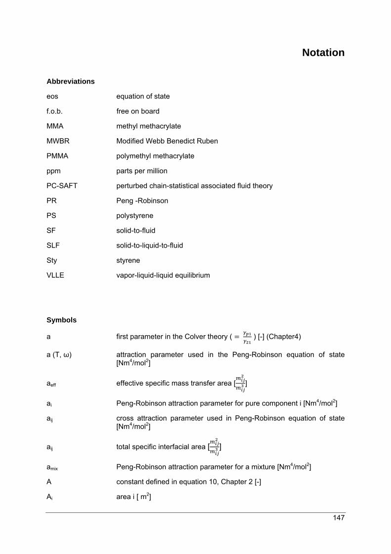
147
Notation
Abbreviations
eos equation of state
f.o.b. free on board
MMA methyl methacrylate
MWBR Modified Webb Benedict Ruben
PMMA polymethyl methacrylate
ppm parts per million
PC-SAFT perturbed chain-statistical associated fluid theory
PR Peng -Robinson
PS polystyrene
SF solid-to-fluid
SLF solid-to-liquid-to-fluid
Sty styrene
VLLE vapor-liquid-liquid equilibrium
Symbols
a first parameter in the Colver theory ( ) [-] (Chapter4)
a (T, ω) attraction parameter used in the Peng-Robinson equation of state [Nm4/mol2]
aeff effective specific mass transfer area [ ]
ai Peng-Robinson attraction parameter for pure component i [Nm4/mol2]
aij cross attraction parameter used in Peng-Robinson equation of state [Nm4/mol2]
aij total specific interfacial area [ ]
amix Peng-Robinson attraction parameter for a mixture [Nm4/mol2]
A constant defined in equation 10, Chapter 2 [-]
Ai area i [ m2]

Notation
148
Ai interfacial area of the ith interface [ m2]
Aassoc Helmholtz energy covering the association contribution [J]
Adisp Helmholtz energy covering the dispersion contribution [J]
Ahc Helmholtz energy covering the hard chain contribution [J]
Apert Helmholtz energy covering the perturbation contribution [J]
Aref Helmholtz energy of the reference system [J]
Ares residual Helmholtz energy [J]
b second parameter in the Colver theory ( ) [-] (Chapter 4)
b volume parameter used in the Peng-Robinson equation of state [m3/mol]
bi Peng-Robinson volume parameter for pure component i [m3/mol]
bmix Peng-Robinson volume parameter for a mixture [m3/mol]
B constant defined in equation 11, Chapter 2 [-]
C constant factor
CD drag coefficient [-]
C0 monomer concentration in the center of the polymer particle [ ]
CP,i specific heat of phase i [°
]
Cs monomer concentration at the surface of the polymer particle [ ]
Cmoni equilibrium monomer concentration in phase i [mol monomer / kg phase i]
Dc column diameter [m]
di diameter of sphere i [m]
dparticle diameter of polymer particle [m]
diffusion coefficient of monomer m in phase i [ ]
fi fugacity of a pure component i [Pa]
fi fugacity of component i in a mixture [Pa]
fi° standard fugacity of component i [Pa]
fin fugacity of component i in phase n [Pa]
FB buoyant force [N]
FD drag force [N]

Notation
149
FG external force [N]
Fo Fourier number [-]
g gravitational force [m/s²]
G0 total energy of a solid-liquid-liquid system [-]
Gm molar Gibbs free energy [J mole-1]
Gi° standard molar Gibbs energy [J mole-1]
GmE excess molar Gibbs energy [J mole-1]
∆G Gibbs free energy change [J]
∆Gi energy difference of phase I with respect to the minimal energy [-]
∆mixGm molar Gibbs energy of mixing [J mole-1]
∆mixGm, id molar Gibbs energy of mixing to form an ideal mixture [J mole-1]
∆∆Gsolution difference in Gibbs free energy of solution of monomer dissolved in CO2 and of monomer dissolved in CO2 swollen polymer [J mole-1]
h enthalpy per kg [kJ/kg]
Hc column height [m]
Hc, n column height when n ppm residual monomer is reached
HHETP height equivalent of a theoretical plate [m]
Hm enthalpy of mixing [J mole-1]
Hi° standard enthalpy [J mole-1]
∆∆Hsolution difference in heat of solution of monomer dissolved in CO2 and monomer dissolved in CO2 swollen polymer [ J mole-1]
kb Boltzman constant, 1.38 * 10-23 [ ]
partial mass transfer coefficient of monomer in phase i [ ]
kij binary interaction parameter accounting for the interaction of unlike molecules [-]
Ki partition coefficient of monomer i between (sc)CO2 and polymer i [kg polymer/ kg (sc)CO2]
Kmon partition coefficient of monomer between (sc)CO2 and polymer [kg polymer/ kg (sc)CO2]
K partition coefficient of monomer between the (sc)CO2 and polymer at temperature Ti [kg polymer/ kg (sc)CO2]
lBF mean free path of base fluid ( 0.17 nm) [m]
m number of segments [-]

Notation
150
msphere mass of sphere [kg]
Mi mass of species i [kg]
Mw weight averaged molecular weight [kg/mol]
Nts number of theoretical stages [-]
n total number of molecules [-]
ni number of molecules of component i [-]
P pressure [Pa]
PA attractive term of pressure [Pa]
Pc critical pressure [Pa]
PR repulsive term of pressure [Pa]
Ptotal total pressure of the system [bar]
p(I) coefficient number I, defined in Appendix B, Chapter 3
P monomer saturated vapor pressure [bar]
R gas constant [8.314 J mole-1 K-1]
Re Reynolds number [-]
RP polymer particle radius [m]
rp polymer particle radius [m]
rs steam flow rate [kg steam/kg dry solids s] (from personal communication)
s isentropy [kcal/°C]
∆s distance a particle travels in the interfacial region [m]
Si spreading coefficient of phase i [-]
Si° standard entropy [J mole-1 K-1]
Sh Sherwood number [-]
Sm entropy of mixing [J mole-1 K-1]
tcontact, i contact time of phase i [s]
T temperature [K]
Tc critical temperature [K]
Tg glass transition temperature [K]
Tr reduced temperature [-]
∆Tln logarithmic mean temperature difference [K][

Notation
151
u internal energy [kJ/kg]
U overall heat transfer coefficient [ °]
v molar volume [m3/mol]
vBr Brownian velocity of the polymer particles [ ]
vc superficial velocity of the continuous phase [ ]
vd superficial velocity of the dispersed phase [ ]
vi molar volume of component i [m3/mol]
vs slip velocity [ ]
v∞ hindered rising velocity of one bubble [ ]
V volume [m³]
xi molar fraction of component i in the liquid phase [-]
X conversion [-]
yi molar fraction of component i in the vapor phase [-]
wi weigth fraction of component i [-]
Z compressibility factor, defined in equation 12 [-]
z particle’s position with respect to the interface [m]
z0 ratio of the particles position with respect to the interface over the particle radius [-]
z particle’s equilibrium position (= b - a) [-]
Greek letters
ai activity of component i [-]
boundary layer thickness of phase i [m]
εd dispersed phase hold up
⁄ energy related to the interaction of two segments [K]
fugacity coefficient of component i in phase I [-]
mass flow rate of phase i kg
hr or
kg
ϕ heat flow kW

Notation
152
ϕ , shaft work kW
Φ polymer volume fraction [-]
activity coefficient of component i [-]
interfacial tension between phase i and j [ ]
monomer activity coefficient [-]
thermal conductivity coefficient [°
]
dynamic viscosity of H2O [Pa s]
μi chemical potential of component i [J mole-1]
μi° standard chemical potential of component i [J mole-1]
μiE excess chemical potential of component i [J mole-1]
μi, id chemical potential of component i of an ideal mixture [J mole-1]
ρ density
size of segments [Å]
residence time of CO2 bubbles in the column when n residual monomer level is reached [s]
fraction of the interfacial area covered with polymer particles [-]
ω acentric factor [-]


155
Dankwoord
Aan het einde van mijn promotieonderzoek kan ik terugkijken op een intensieve, leerrijke en
aangename periode in mijn leven. Natuurlijk zijn er heel veel mensen die hier op een of
andere manier toe hebben bijgedragen en ik wil hen dan ook graag bedanken.
Allereerst wil ik mijn promotor Jos Keurentjes bedanken voor de mogelijkheid dit ongelofelijk
interessante promotieonderzoek uit te voeren. Dankjewel voor je vertrouwen en
aanmoedigingen, voor je enthousiasme en klare kijk op zoveel dingen. Ik heb genoten van
onze gesprekken, zowel binnen als buiten het project, waardoor ik altijd weer een duidelijke
en open visie kreeg om de toekomst met vernieuwd enthousiasme tegemoet te gaan.
Ook wil ik graag mijn dagelijkse begeleiders bedanken. In het eerste deel van de promotie
was Maartje Kemmere hierin de aandrijvende kracht. Maartje, ik heb veel van je geleerd,
zowel op professioneel als op persoonlijk vlak. Dankjewel, ik zal je nooit vergeten. Jan
Meuldijk werd mijn nieuwe toeverlaat, een keuze die heel snel gemaakt werd. Jan, zoals je
zelf dikwijls hebt vermeld, hebben we ondertussen al een heel verleden samen. Van het
allereerste begin in Diepenbeek, april 2001, tot nu heb ik genoten van onze samenwerking
en jouw enorme kennis. Ook je bezorgdheid toen ik het moeilijker had, en vooral je positieve
kijk, stel ik enorm op prijs. Ik kijk ernaar uit om nog veel met jou te mogen samenwerken.
Dan zijn er nog de enthousiaste studenten die aan dit project hebben meegewerkt. Inge, Tijl,
Roel, Rob, Harro, Kirill, Willeke, Judith en Simone, hartelijk dank voor jullie inzet.
Chris, Dolf en Erik, bedankt voor jullie hulp om mijn opstelling draaiende te houden.
Dank aan mijn collega’s van SPD voor de fijne sfeer, zelfs wanneer we in aantal
verminderden. Ik heb veel gelachen en plezier beleefd. Speciale dank aan mijn paranimfen,
Fabiènne en Carin, collega’s en vriendinnen. Jullie weten wat jullie voor mij betekend hebben
tijdens de promotie en daarnaast. Danku!
Tot slot een dank aan mijn familie. Mama, papa, Anja, Michele, Nele en Livio, bedankt voor
jullie ondersteuning en onaflatende interesse in mijn werk en natuurlijk ook de fijne
momenten van ontspanning die zeker nodig waren! Moeke en papa, danku voor alles wat
jullie me gegeven hebben. Wat ik ook bereikt heb in mijn leven, op welk gebied dan ook, heb
ik aan jullie steun en liefde te danken. Danku voor de mogelijkheden die ik heb gekregen,
voor de aanmoedigingen, voor alle levenslessen, danku voor alles. Ook mijn lieve Paulien wil
ik danken om in mij te geloven. Je bent een prachtig persoon die heel veel te geven heeft. Ik
ben er fier op jouw zus te zijn!
Steve, jij bent mijn toeverlaat, mijn leven, mijn beste vriend. Tijdens de mooie momenten was
je er, maar nog meer tijdens de moeilijke momenten. Mijn leven delen met jou maakt de
wereld zoveel mooier…en het beste moet nog komen.


157
Curriculum Vitae
Marijke Aerts was born on January 2nd 1982 in Hasselt (Belgium). In 2000, she finalized her
secondary education at Lyceum (Atheneum III) in Hasselt. In October of that year, she
started studying chemistry at Hasselt University (Diepenbeek, Belgium). After completion of
her second year candidature in 2002, she continued her education in chemical engineering
at the Department of Chemical Engineering and Chemistry of the Eindhoven University of
Technology (The Netherlands). She performed her MSc graduation project entitled
“Synthesis of polyurethanes with carbon dioxide” in the Process Development Group. In
August 2005 she received her MSc degree in Chemical Engineering. From October 2005 till
December 2010, she performed a PhD graduation project in the Process Development
Group under supervision of prof.dr.ir. J.T.F. Keurentjes and prof.dr. J. Meuldijk. The subject
of the project was reduction of residual monomer in polymer latex products with high
pressure carbon dioxide. The results of this research project sponsored by the Foundation
Emulsion Polymerization, are summarized in this thesis. As from September 1st 2011, she is
working as a process development engineer at Bodec Process Technology in Best (The
Netherlands).