Embed Size (px)
Citation preview
Residential choice, the built environment, and non-work travel: Evidence using new data and methods Submitted to Environment and Planning A Additional minor changes, April 29, 2008 Daniel G. Chatman, Ph.D. Bloustein School of Planning and Public Policy Rutgers University 33 Livingston Ave, Suite 302 New Brunswick, NJ 08901 [email protected] 732.932.3822 x724 732.932.2253 (fax) Dan Chatman is an assistant professor of urban planning at Rutgers University. Acknowledgments – Many thanks to Randy Crane, Mike Manville, Bob Lake, Mike Greenberg, Bill Rodgers, Ken Small, and three anonymous reviewers for their detailed comments and suggestions. The planning and implementation of the survey and the subsequent data cleaning and construction of built environment measures was funded by the California Department of Transportation, through a contract managed by Terry Parker. The survey was carried out by telephone interviewers from M. Davis & Company of Philadelphia. Thanks to Jim Brown, Morris Davis and other staff at that firm. This article is a significantly modified version of a chapter of my dissertation, funding support for which was provided by the Federal Highway Administration’s Eisenhower Fellowship, the University of California Chancellor’s Fellowship, and the Department of Urban Planning at UCLA.

Residential choice and non-work travel: Evidence using new data and methods Dan Chatman
2
Residential choice and non-work travel: Evidence using new data and methods Dan Chatman
3
Residential choice and non-work travel: Evidence using new data and methods
Abstract. Residents of dense, mixed-use, transit-accessible neighborhoods use autos less. Recent studies have suggested that this relationship is partly because transit- and walk-preferring households seek and find such neighborhoods. If so, and if the number of such households is small, policies to alter the built environment may not influence auto use very much. I argue that many of these studies are inconclusive on methodological grounds, and more research is needed. Here a purpose-designed survey of households in two urban regions in California is investigated using a new methodological approach. I find that most surveyed households explicitly consider travel access of some kind when choosing a neighborhood, but this process of residential self-selection does not bias estimates of the built environment’s effects very much. To the extent that it does, the bias results in both underestimates and overestimates of the built environment’s effects, contrary to previous research. The analysis not only implies a need for deregulatory approaches to land use and transportation planning, but also suggests that there may be value in market interventions such as subsidies and new prescriptive regulations.
Residential choice and non-work travel: Evidence using new data and methods Dan Chatman
4
1. Introduction
People who live in densely-developed, transit-served neighborhoods with shops
and services near their homes tend to walk and use transit more, and own and use autos
less, than people who live in auto-oriented neighborhoods. Many planners and academic
researchers have therefore argued for policies to encourage denser development, with a
greater mix of uses, particularly near major transit stops. But this correlation between the
built environment and auto use may be misleading, and if so, such policies might not
have the intended effects.
The residential self-selection hypothesis, as conventionally framed, is as follows
(e.g., Schimek 1996; Badoe and Miller 2000; Bento et al. 2001; Boarnet and Crane
2001). Households choose neighborhoods based on their expected travel patterns.
Transit-seeking households are more likely to buy or rent homes near a stop on the line to
work; people who shop a lot by car are more likely to find a place to live near a highway
on-ramp; households who like to walk to the park choose neighborhoods with good parks
within walking distance. This sorting process, if not statistically controlled, confounds the
estimation of the neighborhood built environment’s effects upon household travel.
because if variation in the built environment leads to households spatially sorting
themselves according to their travel preferences, then those preferences will be highly
correlated with built environment characteristics.
But there are two more implicit parts of the residential self-selection hypothesis.
The first is that people who seek accessible neighborhoods generally find them. If they
did not, the correlation between pre-existing travel preferences and built environment
Residential choice and non-work travel: Evidence using new data and methods Dan Chatman
5
characteristics might not be strong enough to significantly bias estimates of the built
environment's effects on travel. In addition, there would be an argument for deregulatory
policies precisely to encourage more residential self-selection (Levine 1998).
The second implicit part is that a select group of willing households is reliant
upon the built environment to “express their preferences” to use transit and to walk, while
the remainder of the population is less responsive to built environment variation. But the
opposite is also possible. People who like to walk might be more willing to walk longer
distances; people who like to drive might not be dissuaded by traffic congestion caused
by dense development; and so on.
Thus the residential self-selection hypothesis is, in a nutshell, really three non-
mutually-exclusive hypotheses: (1) people decide where to live based on how they expect
to travel (and their predictions are correct), (2) this sorting process is not significantly
constrained, so preferences and built environment characteristics are highly correlated,
and (3) self-selecters are more responsive to the built environment.
The truth or falsity of these hypotheses will likely vary by urban area, with
differing policy implications. If the relationship between travel and the built environment
depends on alternative-mode-seeking households living in dense, transit-accessible
places, then the argument for government intervention depends on the size of that group,
and whether the supply of such neighborhoods is significantly constrained. If households
predisposed to use alternative travel modes already find neighborhoods that match their
preferences, policy interventions may not make much of a difference. But it could be that
a significant share of households seeking accessible neighborhoods is unsuccessful due to
Residential choice and non-work travel: Evidence using new data and methods Dan Chatman
6
land use regulations that constrain the supply of those neighborhoods. In that case one
policy solution would be to relax those constraints, particularly in targeted areas (e.g.,
near transit stops). Finally, if the built environment influences even habitual auto users to
use autos less, a more wide-scale adoption of policies to alter development patterns or
relax policy constraints on development may be appropriate, and the argument for
development subsidies and prescriptive regulation is strengthened.
This study builds upon existing literature, employing new methods of data
collection and analysis. Households in two metropolitan areas in California, San Diego
and the San Francisco Bay Area were surveyed. The data are used to analyze the
relationships between the built environment, non-work travel frequency by mode, and
residential choice. This study focuses on non-work travel because non work travel is a
substantial majority of household travel in the United States, accounting for 81 percent of
trips and 73 percent of distance traveled in the most recent nationwide survey of travel,
the 2001 NHTS (Hu and Reuscher 2004).
2. Theory
Empirical evidence strongly suggests that households simultaneously choose their
housing unit and neighborhood along with the anticipated mode and duration of their trip
to work (e.g., Lerman 1976; van Ommeren, Rietveld, and Nijkamp 1999; Cervero and
Duncan 2002), although other criteria can dominate choices for some households
(Giuliano 1991). Do households also choose where to live based on access to non-work
activity locations—such as parks, shops, doctors’ offices, movie theaters, and child care
establishments? As long-distance commuting has become less difficult with improved
Residential choice and non-work travel: Evidence using new data and methods Dan Chatman
7
automobile technology (Rouwendal and Nijkamp 2004), and work trips comprise a
diminishing share of household travel, perhaps non-work travel does have a greater
influence on residential choice. But three main factors discussed below—bundling, the
investment characteristics of homes, and supply constraints—imply that non-work travel
preferences are not likely to play a dominant role.
First, housing is purchased jointly with neighborhood goods, local goods, and
accessibility to activities (e.g., Goodman 1989; Mills and Hamilton 1989). Non-travel
goods in the bundle include the crime rate, municipal services, school quality, the
racial/ethnic mix, and microclimate (Tiebout 1956; Giuliano 1991; Giuliano and Small
1993; Wachs et al. 1993). A preferred rank ordering for all of these choice dimensions
may be impossible (cf. Arrow 1963), and the complexity of the decision may lead
households to prioritize a few salient characteristics (e.g., a safe neighborhood) and
ignore less important ones, in a process of “satisficing” (Simon 1957). For some
households travel accessibility will not be a priority.
Second, homeowners must take into account the resale value of the house which
depends partly on how others value its characteristics (Fischel 2001; Fennell 2006). This
makes it somewhat less likely that transit- and walk-preferring households are willing to
pay a premium for transit and walk access, because they are likely in the minority.
Third, the supply of neighborhoods with high non-work travel accessibility via
alternative modes—as measured by higher development density, proximity to shops,
proximity to transit, dense street grids, and proximity to job centers—may be
significantly constrained in housing markets with strict land use regulations such as San
Residential choice and non-work travel: Evidence using new data and methods Dan Chatman
8
Diego and the San Francisco Bay Area (see, e.g., Cervero 1989; Levine 1998; Glaeser
and Gyourko 2002; Levine, Inam, and Torng 2005). Any such constraint on supply is
likely to lower the probability that households who prefer walk or transit access to non-
work activities manage to locate in such neighborhoods.
3. Empirical literature
Recent research has not resolved the extent to which correlations between
residential built environment characteristics and household non-work travel reflect a
function of a market-sorting process or are an independent function of the built
environment. Four kinds of research design are employed: analyses of land value and
travel accessibility; simultaneous models of residential location and travel; studies of
travel behavior before and after residential moves; and studies using reported attitudes as
measures of travel preferences.
Land value studies can provide indirect support for the hypothesis that people
choose where to live based on access to retail and other non-work destinations, in the
form of evidence whether households pay more for proximity to those destinations. The
evidence here is mixed. For example, Song and Knaap (2003) found that commercial
proximity, land use diversity, and ease of walking increase property values, while Srour,
Kockelman and Dunn (2002) found no evidence of a relationship between residential
land value and walking access to parks and shops.
The second approach relies upon multiple-equation estimation to model the
household’s joint choice of where to live, and how to habitually travel. Boarnet and
Sarmiento (1998) Boarnet and Crane (2001), and Khattak and Rodriguez (2005) all used
Residential choice and non-work travel: Evidence using new data and methods Dan Chatman
9
the instrumental variables approach to create “predicted values” for built environment
characteristics that are based on a first-step equation modeling residential choice. Boarnet
and Sarmiento (1998) and Boarnet and Crane (2001) found that their predicted measures
were substantially less statistically significant than the uncorrected measures, implying
that the built environment influences non-work auto trip frequency only via a process of
residential self-selection. In contrast, Khattak and Rodriguez (2005) found that their
predicted values for a binary “neotraditional” variable did not change results much in
comparison to observed values.
The instrumental variables technique has its problems, chief among which is
reduced efficiency (resulting in lower levels of statistical significance), and the difficulty
of finding appropriate instruments (Gujarati 1995: 604-605). Boarnet and Crane (2001)
test their instruments and find they are statistically appropriate in only one case. Khattak
and Rodriguez (2005) do not report carrying out a test, but they apply the technique using
a variable (“neotraditional”) that takes on only values of 0 and 1 which likely leads to
relatively little variance between predicted and observed values.
Using a nested logit simultaneous model of activity scheduling and residential
location with a one-day activity diary from Massachusetts, Ben-Akiva and Bowman
(1998) found empirical evidence that neighborhood choice was conditioned on
anticipated activity schedules, implying that non-work travel preferences may play a
strong role in residential location choice. Bagley and Moktharian (2002) employ a
structural equations model (SEM) of commute and non-work travel, the built
environment, and travel-related attitudes (as discussed in more detail below). While the
Residential choice and non-work travel: Evidence using new data and methods Dan Chatman
10
SEM method is promising because it can account for mutual causality, the results are
often difficult to interpret, variables must conform to the assumption of normality or be
transformed, and in this case (as sometimes occurs with SEMs) the estimation routine
required significant truncation of the dataset.
The third approach has investigated household travel before and after a move.
With data from the Puget Sound Transportation Panel, Krizek (2003) found that higher
neighborhood and regional accessibility after moving were associated with lower vehicle
distance traveled, a greater number of vehicle tours, and a lower number of stops per
vehicle tour. Based on a survey in Northern California, Handy, Cao and Mokhtarian
(2006) found that residents reported walking more frequently after moving into
neighborhoods that they said were more accessible than their previous neighborhoods.
The before-and-after approach does not test the residential self-selection
hypothesis directly, although it can be combined with other methods. One cannot know
whether alternative-mode-preferring households sought neighborhoods enabling the new
travel patterns, or whether the moves were largely unrelated to the travel accessibility of
the new neighborhood. This approach may show that movers alter their travel behavior
when moving to certain environments, or that changes in the built environment due to a
move are associated with changes in travel behavior, but the method cannot by itself
account for the possibility that movers seek out such environments.
The fourth approach is the reported-attitudes strategy, in which answers to
questions about household attitudes and preferences relating to travel are used as proxy
variables to control for residential self-selection. Mokhtarian, Cao, Schwanen, Handy,
Residential choice and non-work travel: Evidence using new data and methods Dan Chatman
11
and co-authors have used this strategy in combination with structural equations and
quasi-longitudinal approaches (Kitamura, Mokhtarian, and Laidet 1997; Bagley and
Mokhtarian 2002; Schwanen, Dieleman, and Dijst 2004; Schwanen and Mokhtarian
2004; Schwanen and Mokhtarian 2005; Cao, Handy, and Mokhtarian 2006; Handy, Cao,
and Mokhtarian 2006; Cao, Mokhtarian, and Handy 2007). I discuss two early studies
from this set. Using data from households in five San Francisco Bay Area neighborhoods,
Kitamura, Mokhtarian and Laidet (1997) initially found statistically significant
relationships between the built environment characteristics of people’s neighborhoods
and their trip-making and mode choices. However, when measures of respondent
attitudes toward travel and residential location were included, the built environment
measures declined in significance. Bagley and Mokhtarian (2002) estimated a structural
equations model of commute and non-work travel by mode. Two attitude variables were
modeled as a function of the built environment and travel, while a large number of others
were treated as independent, including whether the household believed that having shops
and services near home is important; that public transportation is a good option in
situations when driving is too expensive; and that driving alone is preferable. Many of
these attitudinal variables were significantly related to distance traveled by mode, while
only in one case were either of the two built environment factors significantly related to
travel. In a somewhat different implementation of the strategy, Khattak and Rodriguez
(2005) use reported attitudes as instruments in a first-stage equation predicting whether
households choose to live in a neotraditional neighborhood. These variables include
responses to questions about whether having a back yard is important, whether it is nice
Residential choice and non-work travel: Evidence using new data and methods Dan Chatman
12
to have a house near the sidewalk, and whether new development consumes too much
land.
The reported-attitudes strategy is problematic because stated attitudes of
households about travel, travel-related topics, and the built environment could themselves
be influenced by characteristics of the neighborhoods that the households have chosen, as
well as by people’s travel behavior in the new neighborhood. First, people may alter their
attitudes, or their reports of their attitudes, to be consistent with their chosen
neighborhoods, in response to “cognitive dissonance” (Festinger 1957). Experiments by
social psychologists have shown that “after making important decisions, we usually
reduce dissonance by upgrading the chosen alternative and downgrading the unchosen
option” when asked to rate alternatives before and after making a choice (Myers 2002:
151). Rather than attitudes causing behavior, people will often change their attitudes
when their attitudes conflict with their behavior.
The relevance of cognitive dissonance in travel behavior and travel-related
attitudes has been shown empirically. A Los Angeles study employing simultaneous
equations models showed that perceptions of the attributes of transit buses influenced,
and were influenced by, habitual commute mode. Under one specification, behavior
influenced attitudes but the initial effect of attitudes on mode choice was rendered
statistically insignificant in the simultaneous model (Reibstein, Lovelock, and Dobson
1980). A study near Amsterdam showed evidence that solo driver attitudes about
carpooling were negatively influenced by construction of a new carpool lane, implying a
process of cognitive dissonance or self-justification (VanVugt et al. 1996). In another
Residential choice and non-work travel: Evidence using new data and methods Dan Chatman
13
study in the Netherlands, respondents confronted with the estimated environmental
impacts of their auto driving over an eight-week period were more likely to alter their
reported attitudes to be less “pro-environment” than to commit to changing their driving
habits (Tertoolen, van Kreveld, and Verstraten 1998).
In addition to the influence of travel habits on attitudes, attitudes may also
genuinely change over time either because of new travel habits, due to exposure to a new
environment, or due to changes in the household (e.g., Schwanen and Mokhtarian 2004).
The net result of cognitive dissonance and of other changes in attitudes is that households
may be more likely to report that “having shops and services close by is important to me”
if they have ended up living in a place with shops and services close by, even if they
chose the neighborhood for unrelated reasons.
Reported attitudes and preferences about travel or about the current neighborhood
and built environment may both be influenced by cognitive dissonance in a way that can
bias analysis—not only if travel attitudes are affected by current travel habits, but also if
neighborhood or built environment attitudes are influenced by the chosen built
environment, and if the built environment influences travel. Thus, like attitudes about
travel, attitudes about the built environment (or about sprawl, or about neighborhoods)
cannot be treated as independent influences on travel.
4. Research design
The research method employed here is a variant on the reported-attitudes
approach described above. I surveyed households about how they decided where to live
at the time of their most recent move, and their travel for a 24-hour period. Respondent
Residential choice and non-work travel: Evidence using new data and methods Dan Chatman
14
answers to the questions about the residential search process were used to construct
variables representing pre-move preferences. The cognitive dissonance phenomenon is
elicited when people are confronted with a conflict between the values they hold and their
actual behavior, and the questionnaire aims to reduce that conflict. The questions to elicit
residential choice criteria are asked before questions about travel, and the questions
themselves elicit previous search criteria rather than current preferences. Both differences
should produce measures that more closely track pre-move travel preferences both
because they are less subject to post-move changes in preferences that are caused by the
built environment itself, and because they are less subject to alterations in reports of
current preferences caused by cognitive dissonance.1
These attempts to reduce cognitive dissonance may not be entirely successful. But
the expected direction of any residual analytical bias due to cognitive dissonance is clear.
Like current reported preferences, contemporaneously-reported search criteria will be
more highly correlated with travel behavior and the current residential environment than
criteria at the time of the search. Therefore cognitive dissonance will cause false
negatives, not false positives, when measuring built environment influences; that is,
findings of statistical insignificance of built environment variables are less reliable than
are findings of statistical significance.
1 Handy, Cao and Mokhtarian (2006) and Cao, Mokhtarian and Handy (2007) include questions about “preferred neighbourhood characteristics” “when looking for a new place to live,” in addition to questions about attitudes toward travel. It is not clear whether these questions explicitly elicited search criteria at the time of the most recent move. These variables are not substituted for attitudinal variables in the models, but are employed along with them.
Residential choice and non-work travel: Evidence using new data and methods Dan Chatman
15
4.1. Data
A computer-aided telephone survey was administered between November 2003
and April 2004 to a stratified random sample of households living in the San Diego
metropolitan area and in the three core counties of the San Francisco-Oakland-San Jose
metropolitan area. The design included an over-sample of households living near twelve
selected rail stations in the two metropolitan areas (for details on station area selection,
see Chatman (2005: 199-217)). Respondents without listed telephone numbers in the
station areas were recruited to call a toll-free number while other households were
telephoned directly. The survey collected travel, demographic, and socioeconomic
information, including 24 hours of complete activity data using a retrospective activity
diary format similar to that used in the American Time Use Survey. The interview was
completed by 1,113 adults. Average interview time was 25 minutes, with 10 percent of
the sample requiring more than 40 minutes. Only those respondents who provided
sufficient address information for their homes to be geocoded, and who were responsive
to the questions about residential choice, were included, leaving 999 respondents in the
data set used for analysis.
The survey included questions about what respondents considered when choosing
their current neighborhoods, based in part on questions on the Los Angeles Family and
Neighborhood Survey (Sastry et al. 2000). About 74 percent of households had moved in
the previous ten years (slightly higher than, but comparable to the counties in the study
area, which ranged between 67 and 72 percent as of Census 2000). Follow-up questions
Residential choice and non-work travel: Evidence using new data and methods Dan Chatman
16
determined which travel modes were of interest at that time. Both questions were asked
early in the survey, prior to travel or demographic questions.
The first residential location question was:
When people move, they choose a new house or apartment and also choose a new neighborhood. Please think back to what kind of neighborhood you were hoping to find when you moved in [move year]. What were some things that you looked for? After each response, probe: What else did you look for? If respondent says housing cost or rent was important, probe: Given that you had to find a neighborhood that you could afford, what were some other things that you were looking for?
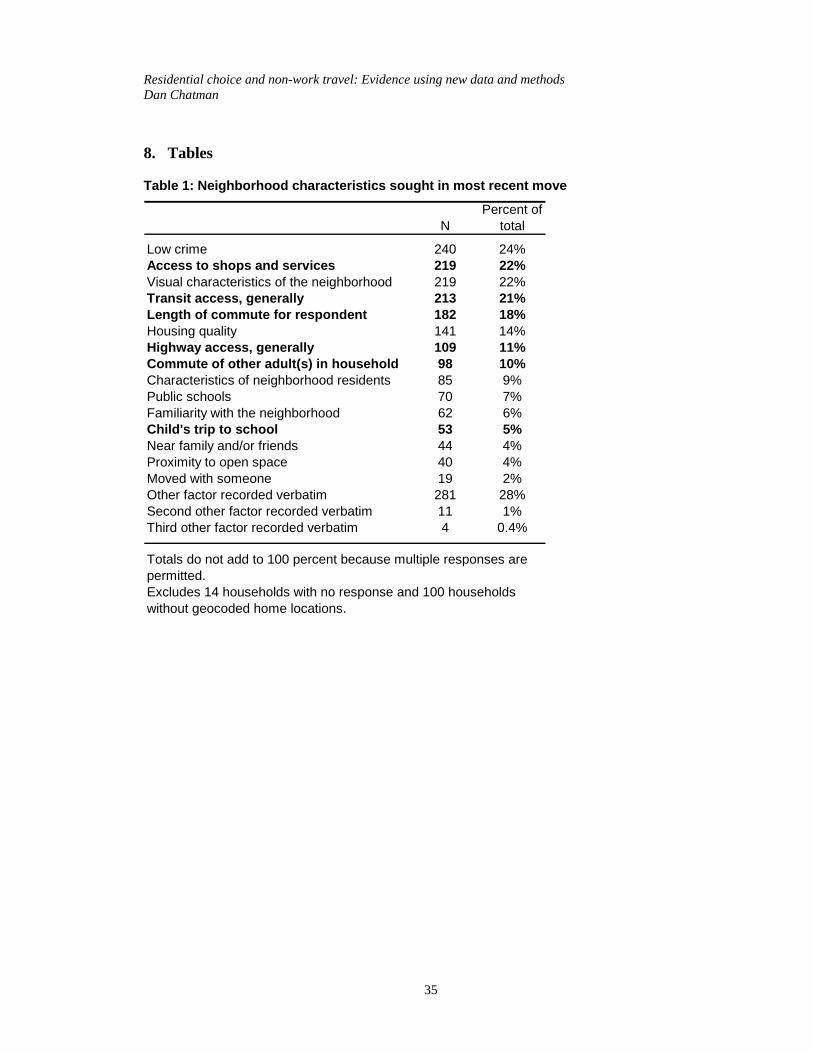
There were 15 precoded responses (see Table 1 for a complete list). Reasons not
falling within these categories were recorded verbatim, and recoded into the relevant
travel-related categories in post-processing.
[Table 1 about here]
The 532 respondents who stated that they prioritized their own commute, the
commute of another household member, a household child’s school trip, or access to
shops/services were asked follow-up questions regarding specific modes—for example:
For your personal commute to school or work, which transportation modes were important considerations in deciding where to live? You may choose more than one. Walking, biking, rail, bus, or personal vehicle (such as a car, van, SUV, pickup truck, RV or motorcycle)?
Multiple responses were allowed to each of the four such follow-up questions,
and were used to create the search criteria variables described in the next section.
Response rates for the metropolitan area strata and station area households with
known telephone numbers ranged between 20 and 24 percent, based on Council of
American Survey Research Organization standards. For those recruited via the mail, the
completion rate was about seven percent (a lower bound of the response rate because it
Residential choice and non-work travel: Evidence using new data and methods Dan Chatman
17
does not account for vacant units or incorrect addresses). The net response rate sample-
wide approaches 20 percent. While the low response rates do present a concern for the
representativeness of the sample for population description purposes, they pose a
substantially less significant concern for the validity of the comparative analysis among
subgroups that is presented here (see, e.g., Groves 1989, p 5). The data were to be used
primarily in estimating differences between subgroups of people, and demographic
characteristics are controlled. More details on the survey, survey dataset and built
environment data sources are available in Chatman (2005: 171-198).
4.2. Dependent variables
The three dependent variables are the number of non-work trips by auto
(including motorcycles and carpools), transit (bus or rail), and walk/bike. Respondents
were asked to provide destination type for all activities during a 24-hour period. They
provided information for about 80 percent of activities outside work, home, or school.
Non-work trips made up 83 percent of those carried out outside home, work, or school;
the remaining 17 percent were pick-up and drop-off trips not otherwise categorizable.
Return trips are excluded from the analysis. For segmented trips, mode is assigned based
on the longest-duration segment.
About 40 percent of respondents did not engage in a non-work activity outside the
home on the survey day, but all respondents are included in the analysis to avoid non-
random sample truncation. The average number of trips to access non-work activities was
1.24, 36 percent of the average total number of trips of 3.42 (which includes return trips
home). Auto and other personal vehicles accounted for 77 percent of non-work trips,
Residential choice and non-work travel: Evidence using new data and methods Dan Chatman
18
much lower than the average for the regions, reflecting the stratified sample which over-
represented transit-proximate, walk-accessible areas.
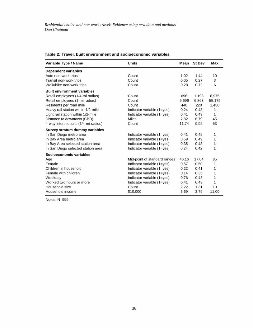
[Table 2 about here]
4.3. Independent variables
Search criteria variables. Respondents’ answers to the residential location
question and to the follow-up questions about specific modes were used to create dummy
variables set equal to one, and otherwise to zero (Table 3, below). For example, if the
respondent reported that the commute to work was an important criterion, and if both
auto and transit were mentioned as relevant modes, then the variables “Sought auto
access for any purpose” and “Sought transit access for any purpose” were set equal to
one, and all others were set equal to zero. In subsequent regression analysis the variables
were sometimes combined, as described below. They were also recoded for some
households in post-processing to account for those verbatim responses not initially
categorized as being travel-access-related.
Built environment variables were measured near the home (geocoded by street
address or in some cases nearest cross streets) using circular buffers. Measures consisted
of the number of retail workers within a 1/4 mile and a one mile radius; residents per road
mile within one-mile; four-way street intersections within 1/4-mile, presence of a heavy
rail station (BART or Caltrain) within 1/2-mile, presence of a light rail station (San Diego
trolley or Santa Clara Valley Transit Authority light rail) within 1/2-mile; distance to the
nearest major central business district (San Diego, San Jose, Oakland, or San Francisco);
and whether there is a sidewalk on both sides of the street (Table 2). All but the self-
Residential choice and non-work travel: Evidence using new data and methods Dan Chatman
19
reported sidewalk measure were calculated in a computationally intensive GIS process
using electronic parcel, Census block, transportation analysis zone, and street maps. See
Chatman (2005) for further details. In addition to these, stratum dummy variables are
included to partly control for any effects of the stratified sample design not captured by
other independent variables (Table 2). These variables show that the sample was 59
percent Bay Area, and 41 percent San Diego County, with Bay Area and San Diego
selected station areas making up 35 and 24 percent of the total respectively.
Control variables include household income; income squared; household size;
sex of respondent; whether children live in the household; an interaction of these two
(female respondent with children in household); whether the person worked outside the
home on the survey day for two hours or more; and whether the survey day was a
weekday (Table 2).
4.4. Model form
Estimating the influences of the built environment and residential preferences on
non-work trip frequency requires a modeling technique that accounts for the discrete
count nature of the dependent variable (Cameron and Trivedi 1998). Here a version of the
negative binomial model is used in which the variance is parameterized as a quadratic
function of the expected mean.
Although not a simultaneous modeling process, a set of count models has
advantages. Unlike a multinomial mode choice model, it takes into account both the share
and the number of trips by each mode, and can be used to investigate mode substitution
Residential choice and non-work travel: Evidence using new data and methods Dan Chatman
20
and induced travel simultaneously. It is not as prone to respondent error as is a model of
distance traveled (e.g., a VMT model).
The vector of independent variables includes measures likely to directly influence
trip making by one of the three modes, because these measures may have indirect effects
on trip frequency by the other modes. For example, the auto trip frequency model
includes transit access and pedestrian connectivity as independent variables in order to
test whether by increasing trip making by transit and walking, these built environment
characteristics decrease auto trip making. Thus each of the three mode-specific trip
frequency models can be thought of as a reduced form version of a simultaneous system
of equations across modes.
5. Results
Four interrelated research questions are addressed here:
1. What share of households explicitly considers non-work access specifically,
and travel access generally, when choosing where to live?
2. Do households who report seeking neighborhoods with good travel access
successfully find such neighborhoods?
3. Does any residential sorting of households according to travel preferences
confound conventional estimates of the built environment’s effects on travel?
4. Does the built environment have different effects on those with strong and
weak travel preferences?
Residential choice and non-work travel: Evidence using new data and methods Dan Chatman
21
5.1. Who considers travel access when choosing a neighborhood?
Access to shops and services was the second most highly sought-after
neighborhood characteristic, at 22 percent of the sample, just after low crime (24 percent
of the sample) (Table 1, above). “Access to transit” was mentioned by 21 percent of the
sample; the respondent’s commute length, 18 percent; highway proximity, 11 percent;
commute length for another adult in the household, 10 percent; and a child’s trip to
school, 5 percent. In all, slightly more than half of respondents (53 percent) cited travel
access of some kind when asked what they sought when choosing a neighborhood. Since
everyone needs to be within some distance of other people and places, these answers are
best understood as distinguishing households who strongly prioritized travel access from
those who prioritized other criteria.
Households who prioritized travel access were younger, smaller, and had lived in
their homes for 1.8 fewer years on average. They were significantly less likely to mention
the type of people living in the neighborhood (e.g., families with children, people of the
same race/ethnicity), the crime rate, having family and friends nearby, or their familiarity
with the area (based on chi-squared tabular frequency tests, not shown here). They were
also less likely to say that they restricted their search to neighborhoods with a particular
kind of housing (e.g., where more apartments or large houses were available). But at the
same time, these households were also substantially more likely to have competing
search priorities. Two-thirds also cited at least one other search criterion, compared to 38
percent of the group that did not cite travel access.
Residential choice and non-work travel: Evidence using new data and methods Dan Chatman
22
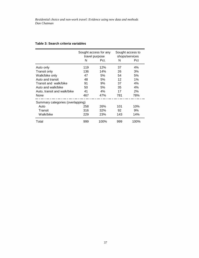
The answers to the follow up questions about travel mode are summarized in
Table 3. Respondents could cite more than one mode; for example, 4 percent of
respondents said they sought auto, transit and walk/bike access for some travel purpose.
Among respondents seeking access for any travel purpose, transit-only seekers made up
the largest group at 14 percent of respondents. (As described above, the survey
oversampled households living near selected rail stops.) Restricting the group specifically
to those who sought access to shops and services, the largest group was those who sought
walk/bike access (5 percent). Summary categories are also shown in Table 3.
[Table 3 about here]
5.2. Do households with strong travel preferences find matching neighborhoods?
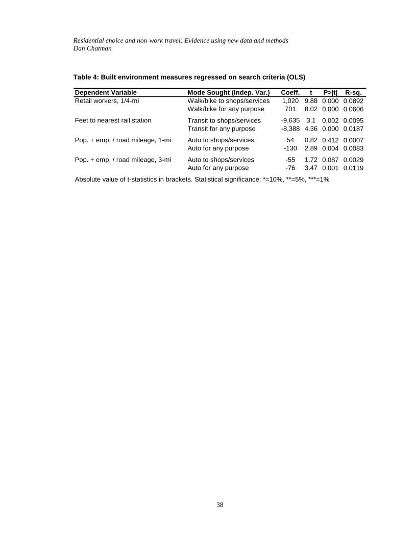
Simple regressions are used to test the correlation between built environment
measures and the share of households reporting that they sought travel access (Table 4).
Possible confounding factors, such as demographic characteristics, are not controlled.
The intention is to determine whether households that report seeking a certain kind of
access obtain such access at a higher rate than those who do not.
[Table 4 about here]
Households who sought good walk or bike access to shops and services live in
neighborhoods with an average of 1,020 more retail workers in the quarter mile area near
home (a one-standard-deviation increase in activity density). Those who sought transit
access to shops or services live an average of 9,635 feet (about 1.8 miles) closer to a rail
stop. Households who sought auto access for any purpose live in areas with 130 fewer
residents per road mile in the mile radius near home (a 1/2-standard-deviation decrease).
Residential choice and non-work travel: Evidence using new data and methods Dan Chatman
23
Finally, 74 percent of households who sought transit access live within a half-mile of a
rail station, versus 58 percent of the remainder (chi-squared 25.6, one degree of freedom,
p-value < 0.001). These regressions show that households who report that they sought
travel access at the time of the most recent move are more likely to live in neighborhoods
with good access via the desired mode, although the relationship is far from
determinative.
5.3. Do access-seeking households travel differently, and does this lead to biased estimates of built environment influences?
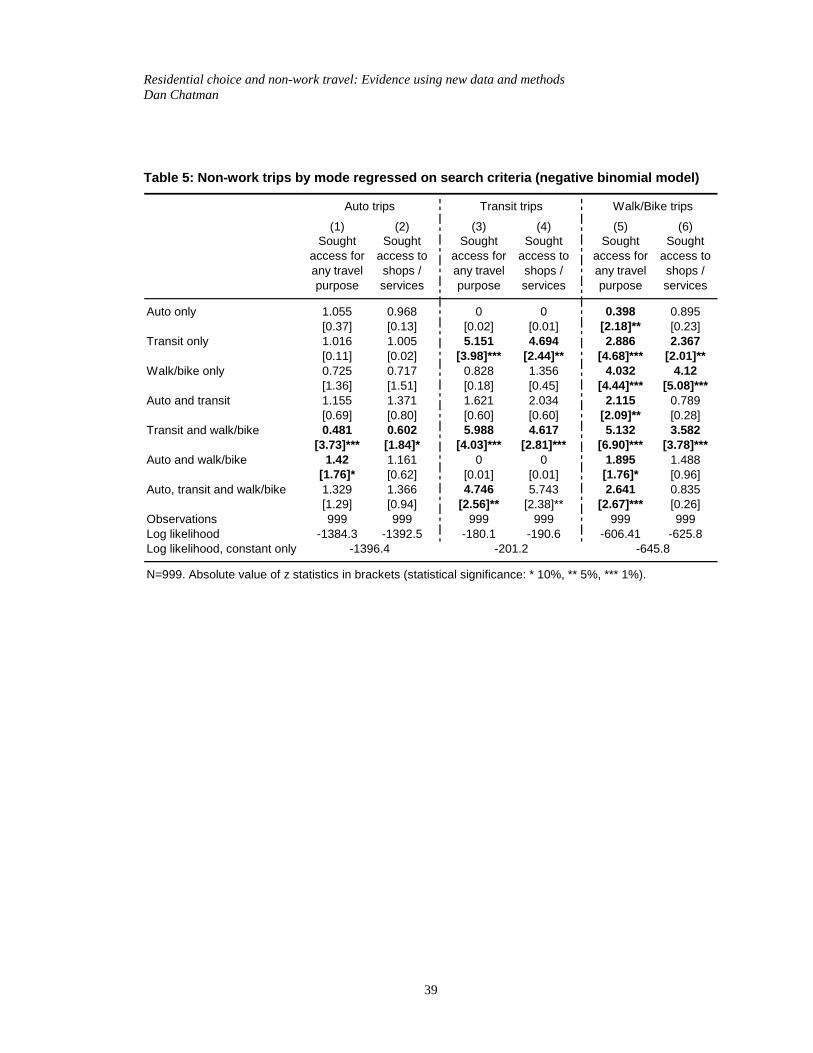
Do access-seeking households travel differently? Results from regressions of trip
frequency by mode on the two sets of search criteria variables (corresponding to the
search criteria summarized in the top portion of Table 3, above) are presented in Table 5.
Exponentiated coefficients (incidence risk ratios) are shown, indicating the relative
frequency of trip making compared to the base group (the “None” category in Table 3).
There are strong relationships between the neighborhood search criteria and the
frequency of non-work trip making by mode. Households seeking walking and bike
access for any purpose make only about half as many auto trips as the base group
(column 1), and those seeking the same type of modal access for shops and services make
about 60 percent as many (column 2), while those who sought both auto and transit
access for any travel purpose make about 40 percent more auto trips (column 1). Those
who sought transit access or transit and walk/bike access make from four-and-a-half to
almost six times the number of transit trips as the base group (columns 3 and 4). And
those who sought walking access (including those who sought it in combination with
some other mode(s)) make between 1.8 and 5.1 times as many walk trips, while those
Residential choice and non-work travel: Evidence using new data and methods Dan Chatman
24
who sought auto access only (for any travel purpose) make just 40 percent as many
walk/bike non-work trips (columns 5 and 6).
[Table 5 about here]
Does the high correlation of travel preferences, as measured by search criteria,
with built environment measures (see Table 4) along with the high correlation of those
pre-existing preferences with observed travel (Table 5), lead to biased estimates of the
built environment’s influences on travel? This question is addressed in the next step of
the analysis, which simultaneously controls for pre-existing travel preferences, built
environment measures and socioeconomic characteristics.
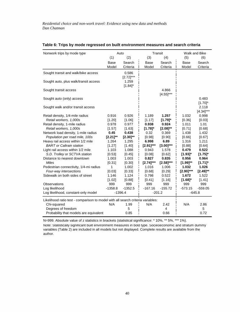
We begin with regressions of personal vehicle, transit, and walk/bike trips on built
environment measures and socioeconomic controls, then add a parsimonious set of the
preference dummy variables to those regressions (Table 6). Only variables that are
statistically significant in at least one of the models are shown. Socioeconomic control
variables are not discussed. The models are built using the set of seven “any travel
purpose” search criteria variables (first columns of Table 3), as those variables are more
highly significant (as shown in Table 5) and more relevant than the more narrowly
defined “shops-and-services” search criteria variables.
For the models shown in columns 2, 4 and 6 of Table 6, the set of seven search
criteria variables is winnowed down to one or two (sometimes combined together as one
variable, e.g., “sought walk or transit access”) based on the analysis shown in Table 5
along with a series of likelihood ratio tests. The final likelihood ratio model tests,
displayed at the bottom of the table, suggest that the models presented here are
Residential choice and non-work travel: Evidence using new data and methods Dan Chatman
25
statistically indistinguishable from models with the full set of preference variables. All
statistically significant search criteria variables are retained, and the omission of the
others hardly affects the coefficients on the built environment variables.
[Table 6 about here]
Accounting for pre-existing travel preferences in this way does not change
measured built environment relationships very much (Table 6). The change in
coefficients for the nine statistically significant built environment measures is in all cases
less than 10 percent, and in all but two cases less than 3 percent. In the base auto trip
model, the only statistically significant built environment measure is the number of
residents per road mile (column 1). This measure is intended to represent road congestion
due to intense development, and is empirically associated with lower road speeds in this
dataset (Chatman Forthcoming). Each additional 1,000 residents per road mile is
associated with 0.45 times as many non-work auto trips (Table 6, column 1), or 55
percent fewer trips. The next model (column 2) includes the two statistically significant
search criteria variables for this model, representing households who sought both transit
and walk/bike access in one group, and households who sought auto along with either
transit access, walk access, or both in the other group. Adding these two statistically
significant search criteria variables to the auto trip model, while improving the model fit,
hardly changes the built environment coefficients.
Non-work transit trip frequency is about six percent lower for each additional
1,000 retail workers in the one-mile radius around home, almost seven times as high
among households with a heavy rail station within one half mile, and 20 percent lower for
Residential choice and non-work travel: Evidence using new data and methods Dan Chatman
26
each mile farther away from the nearest downtown (San Diego, San Francisco, Oakland
or San Jose), where bus service is best (column 3). The model including search criteria
(column 4) shows that all else equal, households who sought some form of transit access
make about five times as many non-work transit trips as the remainder of the population,
but accounting for this preference changes the built environment coefficients very little.
Finally, walk/bike non-work trip frequency is 3.2 percent higher for each
additional four-way intersection within a quarter mile of home (a measure of pedestrian
connectivity); four percent lower for each mile further away from downtown, where
pedestrian-oriented retail uses may be less common; 67 percent higher if there is a
sidewalk on both sides of the street near home; and about 50 percent lower near light rail
stations, which may be less pedestrian-friendly than the metropolitan average (column 5).
Having sought auto access (only) is associated with halving the walk/bike trip frequency
rate, while having sought walk/bike access or transit access is associated with twice the
number of walk/bike trips (column 6). Including these variables changes the built
environment measures somewhat more than in the auto or transit trip frequency models.
The magnitude and statistical significance of the effects is reduced, but in each case less
than 10 percent, and all but the coefficient on the sidewalk variable remain significant at
the 10 percent level or better.
Note that the changes that do occur in the auto and transit non-work trip
frequency models actually marginally increase the statistical significance and the
magnitude of the measured built environment relationships. In these cases, accounting for
residential self-selection with this method seems to result in stronger built environment
Residential choice and non-work travel: Evidence using new data and methods Dan Chatman
27
relationships (although whether the changes themselves are statistically significant is not
tested). The opposite is true for the walk/bike model. The implications are explored in
more detail in the next section.
5.4. Are built environment relationships different for households with strong travel preferences?
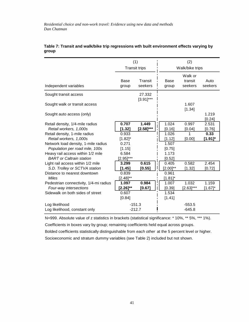
In the final stage of analysis I investigate whether built environment effects
appear to be different for groups of households with different search criteria. The
regression models shown in Table 6 are modified by interacting the search criteria
variables and the built environment measures; those equations are presented in Table 7
(displaying built environment measures only). There are no statistically significant
differences among groups in the auto trip frequency model, even when the most likely
candidates are entered one set at a time, so the auto trip model is not shown.
There are two main findings. First, there are relatively few differences in the
effects of the built environment among households prioritizing travel access and the base
group. Second, in the transit and walk/bike models, there is evidence that some built
environment characteristics have stronger “effects” on the travel of households who did
not seek access by that mode, as well as more conventional evidence that built
environment effects are restricted to households seeking travel access.
[Table 7 about here]
For about half of the built environment variables, the results are so far from
significant that the interactions are dropped entirely from the models. These include
network load density, heavy rail access, and sidewalk availability. For the transit model,
retail density at the one-mile radius is also dropped. The remaining built environment
Residential choice and non-work travel: Evidence using new data and methods Dan Chatman
28
variables are allowed to vary across the two groups, and are boxed in the table.
Coefficients that are statistically different from each other at the 10 percent level or
higher are bolded.
We begin with the transit model. Following the conventional expectation of the
residential self-selection hypothesis, households who sought transit access make 45
percent more transit trips for each additional 1,000 retail workers nearby, while there is
no statistically distinguishable effect for the base group. But those who did not seek
transit access make about 10 percent more transit trips for each additional four-way
intersection near home, while those who did seek transit access are not responsive to
pedestrian connectivity. Meanwhile, light rail access has a larger positive impact on
transit trip making for those who did not seek transit access than for those who did
(although the effect for neither group alone is statistically distinguishable from zero).
In the walk/bike trip model (column 2), the single significant difference is that
higher retail within one mile of home is associated with lower walk/bike trip frequency
among auto-access seekers than the remaining group. Perhaps auto seekers are more
likely to substitute auto for walking when shopping is within a short drive but a long
walk. Some of the remaining results, though not statistically significant, are interesting.
The correlation of walk/bike trips with retail within a quarter mile of home is quite high
for those seeking auto access and nearly absent for those seeking either walk/bike or
transit access. Higher pedestrian connectivity is more highly associated with the
walk/bike trip frequency of those who sought auto access than it is with either those who
Residential choice and non-work travel: Evidence using new data and methods Dan Chatman
29
sought walk/bike access or transit access, or the base group. Again, however, these
statistically insignificant differences are only suggestive.
6. Conclusions
This study adds to a body of research evidence that residential self-selection leads
to mis-estimation of the built environment’s influences on travel. But the measured bias
due to residential self-selection with these methods and data is modest, for the most part
reducing the size of estimated relationships rather than rendering them insignificant. This
study also provides new evidence that households seeking travel access are sometimes
less responsive to the built environment, contrary to the way that the residential self-
selection hypothesis is conventionally framed. Residential self-selection may actually
cause underestimates of built environment influences, because households prioritizing
travel access—particularly, transit accessibility—may be more set in their ways, and
because households may not find accessible neighborhoods even if they prioritize
accessibility.
The empirical models employ a set of seven search criteria dummy variables to
represent travel preferences along with eight more finely-measured built environment
variables. This is in contrast to some previous research that has included a large number
and variety of variables measuring travel-related attitudes, and a smaller number of less
sensitively measured built environment variables. Future research could explicitly test the
sensitivity of results to including more and better measures of pre-existing preferences
and of the built environment.
Residential choice and non-work travel: Evidence using new data and methods Dan Chatman
30
The results are relevant to development policy, though further research is needed
to confirm and expand upon the implications. A deregulatory approach—such as
eliminating height restrictions, low-density residential zoning, parking requirements, and
road level-of-service requirements—may be just a first step, and one insufficient for
significant change in travel behavior in many regions. Where households actively seeking
transit- or walk-accessible neighborhoods are in the minority, the market for such
development may be small.
But the larger group of households that does not seek out walk- and transit-
accessible neighborhoods may be responsive to the built environment nonetheless.
Because this larger share of the population will not demand such development,
prescriptive regulations may be appropriate. Such policies might include maximum
parking requirements, maximum level-of-service road standards, or minimum lot-line
standards, or even restricting the supply of land to drive up its cost and therefore the
density of development. Advocating such policies requires a much more careful
accounting of the social welfare arguments for intervention than can be given here,
including a more explicit assessment of the external costs of auto use, the external
benefits of transit use and walking, and evidence that households’ demand for low-
density, outlying neighborhoods does them more harm than good due to long commutes,
social isolation and sedentary lifestyles.
7. References
Arrow, Kenneth Joseph. 1963. Social choice and individual values. 2nd ed. New Haven: Yale University Press.
Residential choice and non-work travel: Evidence using new data and methods Dan Chatman
31
Badoe, Daniel A., and Eric J. Miller. 2000. Transportation - land-use interaction: Empirical findings in North America, and their implications for modeling. Transportation Research D 5 (4):[235]-263.
Bagley, Michael N., and Patricia L. Mokhtarian. 2002. The impact of residential neighborhood type on travel behavior: A structural equations modeling approach. Annals of Regional Science 36 (2):279-297.
Ben-Akiva, Moshe E., and John L. Bowman. 1998. Integration of an activity-based model system and a residential location model. Urban Studies 35 (7):1131-1153.
Bento, Antonio M., Maureen L. Cropper, Ahmed Mushfiq Mobarak, and Katja Vinha. 2001. The impact of urban spatial structure on travel demand in the United States.
Boarnet, Marlon G., and Randall Crane. 2001. Travel by design: The influence of urban form on travel. New York: Oxford University Press.
Boarnet, Marlon G., and Sharon Sarmiento. 1998. Can land use policy really affect travel behavior? A study of the link between non-work travel and land use characteristics. Urban Studies 35 (7):1155-1169.
Cameron, Adrian Colin, and Pravin K. Trivedi. 1998. Regression analysis of count data, Econometric Society monographs ; no. 30. Cambridge, U.K. ; New York: Cambridge University Press.
Cao, Xinyu Y., Susan L. Handy, and Patricia L. Mokhtarian. 2006. The influences of the built environment and residential self-selection on pedestrian behavior: Evidence from Austin, TX. Transportation 33 (1):1-20.
Cao, Xinyu Y., Patricia L. Mokhtarian, and Susan L. Handy. 2007. Do changes in neighborhood characteristics lead to changes in travel behavior ? A structural equations modeling approach. Transportation 34 (5):535-556.
Cervero, Robert. 1989. Jobs-housing balancing and regional mobility. Journal of the American Planning Association 55 (2):136-151.
Cervero, Robert, and Michael Duncan. 2002. Residential self-selection and rail commuting: A logit analysis (working paper). Berkeley: University of California Transportation Center.
Chatman, Daniel G. 2005. How the built environment influences non-work travel: Theoretical and empirical essays. Dissertation, Department of Urban Planning, University of California, Los Angeles.
Residential choice and non-work travel: Evidence using new data and methods Dan Chatman
32
———. Forthcoming. Deconstructing development density: Quality, quantity and price effects on household non-work travel. Transportation Research Part A: Policy and Practice.
Fennell, Lee Anne. 2006. Exclusion's attraction: Land use controls in Tieboutian perspective. In The Tiebout model at fifty, edited by W. A. Fischel. Washington DC: Lincoln Institute of Land Policy.
Festinger, Leon. 1957. A theory of cognitive dissonance. Stanford: Stanford University Press.
Fischel, William A. 2001. The homevoter hypothesis: How home values influence local government taxation, school finance, and land-use policies Cambridge, Mass.: Harvard University Press.
Giuliano, Genevieve. 1991. Is jobs-housing balance a transportation issue? Transportation Research Record 1305:305-312.
Giuliano, Genevieve, and Kenneth A. Small. 1993. Is the journey to work explained by urban structure? Urban Studies 30 (9):1485-1500.
Glaeser, Edward L., and Joseph Gyourko. 2002. The impact of zoning on housing affordability. Cambridge MA: Harvard Institute of Economic Research.
Goodman, Allen C. 1989. Topics in empirical housing research. In The economics of housing markets, edited by R. Arnott.
Groves, Robert M. 1989. Survey errors and survey costs. New York: John Wiley & Sons.
Gujarati, Damodar N. 1995. Basic econometrics. 3rd ed. New York: McGraw-Hill.
Handy, Susan, Xinyu Cao, and Patricia L. Mokhtarian. 2006. Self-selection in the relationship between the built environment and walking. Journal of the American Planning Association 72 (1):55-74.
Hu, Patricia S., and Timothy R. Reuscher. 2004. Summary of travel trends: 2001 National Household Travel Survey. Washington DC: U.S. Department of Transportation - Federal Highway Administration.
Khattak, Asad J., and Daniel Rodriguez. 2005. Travel behavior in neo-traditional neighborhood developments: A case study in USA. Transportation Research A 39 (6):481-500.
Kitamura, Ryuichi, Patricia L. Mokhtarian, and L. Laidet. 1997. A micro-analysis of land use and travel in five neighborhoods in the San Francisco Bay Area. Transportation 24 (2):125-158.
Residential choice and non-work travel: Evidence using new data and methods Dan Chatman
33
Krizek, Kevin J. 2003. Residential relocation and changes in urban travel: Does neighborhood-scale urban form matter? Journal of the American Planning Association 69 (3):265-281.
Lerman, Steven R. 1976. Location, housing, automobile ownership, and mode to work: A joint choice model. Transportation Research Record 610:6-11.
Levine, Jonathan. 1998. Rethinking accessibility and jobs-housing balance. Journal of the American Planning Association 64 (2):133-150.
Levine, Jonathan, A. Inam, and G. W. Torng. 2005. A choice-based rationale for land use and transportation alternatives - Evidence from Boston and Atlanta. Journal of Planning Education and Research 24 (3):317-330.
Mills, Edwin S., and Bruce W. Hamilton. 1989. Urban economics, 4th edition. Glenview IL: Scott, Foresman and Company.
Myers, David G. 2002. Social psychology. 7th ed. Boston: McGraw-Hill.
Reibstein, David J., Christopher H. Lovelock, and Ricardo de P. Dobson. 1980. The direction of causality between perceptions, affect, and behavior: An application to travel behavior. The Journal of Consumer Research 6 (4):370-376.
Rouwendal, Jan, and Peter Nijkamp. 2004. Living in two worlds: A review of home-to-work decisions. Growth and Change 35 (3):287-303.
Sastry, Narayan, Bonnie Ghosh-Dastidar, John Adams, and Anne Pebley. 2000. The design of a multilevel longitudinal survey of children, families, and communities: The Los Angeles Family and Neighborhood Survey. Santa Monica: RAND.
Schimek, Paul. 1996. Household motor vehicle ownership and use: How much does residential density matter? Transportation Research Record 1552:120-125.
Schwanen, T., F. M. Dieleman, and M. Dijst. 2004. The impact of metropolitan structure on commute behavior in the Netherlands: A multilevel approach. Growth and Change 35 (3):304-333.
Schwanen, Tim, and Patricia L. Mokhtarian. 2005. What affects commute mode choice: neighborhood physical structure or preferences toward neighborhoods? Journal of Transport Geography 13 (1):83-99.
Schwanen, Timothy, and Patricia L. Mokhtarian. 2004. The extent and determinants of dissonance between actual and preferred residential neighborhood type. Environment and Planning B-Planning & Design 31 (5):759-784.
Residential choice and non-work travel: Evidence using new data and methods Dan Chatman
34
Simon, Herbert Alexander. 1957. Models of man: Social and rational; Mathematical essays on rational human behavior in a social setting. New York: Wiley.
Song, Yan, and Gerrit-Jan Knaap. 2003. New urbanism and housing values: a disaggregate assessment. Journal of Urban Economics 54 (2):218-238.
Srour, Issam M., Kara M. Kockelman, and Travis P. Dunn. 2002. Accessibility indices - Connection to residential land prices and location choices. Transportation Research Record 1805:25-34.
Tertoolen, Gerard , Dik van Kreveld, and Ben Verstraten. 1998. Psychological resistance against attempts to reduce private car use. Transportation Research A 32 (3):171-181.
Tiebout, Charles M. 1956. A pure theory of local expenditures. Journal of Political Economy 64:416-424.
van Ommeren, Jos, Piet Rietveld, and Peter Nijkamp. 1999. Job moving, residential moving, and commuting: A search perspective. Journal of Urban Economics 46 (2):230-253.
VanVugt, Mark, Paul A. M. VanLange, Ree M. Meertens, and Jeffrey A. Joireman. 1996. How a structural solution to a real-world social dilemma failed: A field experiment on the first carpool lane in Europe. Social Psychology Quarterly 59 (4):364-374.
Wachs, Martin, Brian D. Taylor, Ned Levine, and Paul M. Ong. 1993. The changing commute: A case-study of the jobs-housing relationship over time. Urban Studies 30 (10):1711.
Residential choice and non-work travel: Evidence using new data and methods Dan Chatman
35
8. Tables
Table 1: Neighborhood characteristics sought in most recent move
NPercent of
total
Low crime 240 24%Access to shops and services 219 22%Visual characteristics of the neighborhood 219 22%Transit access, generally 213 21%Length of commute for respondent 182 18%Housing quality 141 14%Highway access, generally 109 11%Commute of other adult(s) in household 98 10%Characteristics of neighborhood residents 85 9%Public schools 70 7%Familiarity with the neighborhood 62 6%Child's trip to school 53 5%Near family and/or friends 44 4%Proximity to open space 40 4%Moved with someone 19 2%Other factor recorded verbatim 281 28%Second other factor recorded verbatim 11 1%Third other factor recorded verbatim 4 0.4%
Excludes 14 households with no response and 100 households without geocoded home locations.
Totals do not add to 100 percent because multiple responses are permitted.
Residential choice and non-work travel: Evidence using new data and methods Dan Chatman
36
Table 2: Travel, built environment and socioeconomic variables
Variable Type / Name Units Mean St Dev Max
Dependent variablesAuto non-work trips Count 1.02 1.44 10Transit non-work trips Count 0.05 0.27 3Walk/bike non-work trips Count 0.28 0.72 6
Built environment variablesRetail employees (1/4-mi radius) Count 696 1,198 8,975Retail employees (1-mi radius) Count 5,696 6,863 55,175Residents per road mile Count 448 220 1,458Heavy rail station within 1/2-mile Indicator variable (1=yes) 0.24 0.43 1Light rail station within 1/2-mile Indicator variable (1=yes) 0.41 0.49 1Distance to downtown (CBD) Miles 7.82 6.79 454-way intersections (1/4-mi radius) Count 11.74 9.92 53
Survey stratum dummy variablesIn San Diego metro area Indicator variable (1=yes) 0.41 0.49 1In Bay Area metro area Indicator variable (1=yes) 0.59 0.49 1In Bay Area selected station area Indicator variable (1=yes) 0.35 0.48 1In San Diego selected station area Indicator variable (1=yes) 0.24 0.42 1
Socioeconomic variablesAge Mid-point of standard ranges 46.16 17.04 85Female Indicator variable (1=yes) 0.57 0.50 1Children in household Indicator variable (1=yes) 0.22 0.41 1Female with children Indicator variable (1=yes) 0.14 0.35 1Weekday Indicator variable (1=yes) 0.76 0.43 1Worked two hours or more Indicator variable (1=yes) 0.41 0.49 1Household size Count 2.22 1.31 10Household income $10,000 5.69 3.79 11.00
Notes: N=999
Residential choice and non-work travel: Evidence using new data and methods Dan Chatman
37
Table 3: Search criteria variables
N Pct. N Pct
Auto only 119 12% 37 4%Transit only 136 14% 26 3%Walk/bike only 47 5% 54 5%Auto and transit 48 5% 12 1%Transit and walk/bike 91 9% 37 4%Auto and walk/bike 50 5% 35 4%Auto, transit and walk/bike 41 4% 17 2%None 467 47% 781 78%
Summary categories (overlapping)Auto 258 26% 101 10%Transit 316 32% 92 9%Walk/bike 229 23% 143 14%
Total 999 100% 999 100%
Sought access to shops/services
Sought access for any travel purpose
Residential choice and non-work travel: Evidence using new data and methods Dan Chatman
38
Table 4: Built environment measures regressed on search criteria (OLS)
Dependent Variable Mode Sought (Indep. Var.) Coeff. t P>|t| R-sq.Retail workers, 1/4-mi Walk/bike to shops/services 1,020 9.88 0.000 0.0892
Walk/bike for any purpose 701 8.02 0.000 0.0606
Feet to nearest rail station Transit to shops/services -9,635 3.1 0.002 0.0095Transit for any purpose -8,388 4.36 0.000 0.0187
Pop. + emp. / road mileage, 1-mi Auto to shops/services 54 0.82 0.412 0.0007Auto for any purpose -130 2.89 0.004 0.0083
Pop. + emp. / road mileage, 3-mi Auto to shops/services -55 1.72 0.087 0.0029Auto for any purpose -76 3.47 0.001 0.0119
Absolute value of t-statistics in brackets. Statistical significance: *=10%, **=5%, ***=1%
Residential choice and non-work travel: Evidence using new data and methods Dan Chatman
39
Table 5: Non-work trips by mode regressed on search criteria (negative binomial model)
(1) (2) (3) (4) (5) (6)Sought
access for any travel purpose
Sought access to shops / services
Sought access for any travel purpose
Sought access to shops / services
Sought access for any travel purpose
Sought access to shops / services
Auto only 1.055 0.968 0 0 0.398 0.895[0.37] [0.13] [0.02] [0.01] [2.18]** [0.23]
Transit only 1.016 1.005 5.151 4.694 2.886 2.367[0.11] [0.02] [3.98]*** [2.44]** [4.68]*** [2.01]**
Walk/bike only 0.725 0.717 0.828 1.356 4.032 4.12[1.36] [1.51] [0.18] [0.45] [4.44]*** [5.08]***
Auto and transit 1.155 1.371 1.621 2.034 2.115 0.789[0.69] [0.80] [0.60] [0.60] [2.09]** [0.28]
Transit and walk/bike 0.481 0.602 5.988 4.617 5.132 3.582[3.73]*** [1.84]* [4.03]*** [2.81]*** [6.90]*** [3.78]***
Auto and walk/bike 1.42 1.161 0 0 1.895 1.488[1.76]* [0.62] [0.01] [0.01] [1.76]* [0.96]
Auto, transit and walk/bike 1.329 1.366 4.746 5.743 2.641 0.835[1.29] [0.94] [2.56]** [2.38]** [2.67]*** [0.26]
Observations 999 999 999 999 999 999Log likelihood -1384.3 -1392.5 -180.1 -190.6 -606.41 -625.8Log likelihood, constant only
Auto trips Transit trips Walk/Bike trips
N=999. Absolute value of z statistics in brackets (statistical significance: * 10%, ** 5%, *** 1%).
-1396.4 -201.2 -645.8
Residential choice and non-work travel: Evidence using new data and methods Dan Chatman
40
Table 6: Trips by mode regressed on built environment measures and search criteria
Nonwork trips by mode type(1) (2) (3) (4) (5) (6)
Base Model
Search Criteria
Base Model
Search Criteria
Base Model
Search Criteria
Sought transit and walk/bike access 0.586[2.72]***
Sought auto, plus walk/transit access 1.259[1.84]*
Sought transit access 4.866[4.55]***
Sought auto (only) access 0.483[1.70]*
Sought walk and/or transit access 2.118[4.34]***
Retail density, 1/4-mile radius 0.916 0.926 1.189 1.257 1.032 0.998Retail workers, 1,000s [1.20] [1.06] [1.17] [1.79]* [0.36] [0.03]
Retail density, 1-mile radius 0.978 0.977 0.938 0.924 1.011 1.01Retail workers, 1,000s [1.57] [1.63] [1.78]* [2.08]** [0.71] [0.68]
Network load density, 1-mile radius 0.45 0.438 0.32 0.369 1.438 1.432Population per road mile, 100s [2.21]** [2.30]** [0.98] [0.90] [0.66] [0.67]
Heavy rail access within 1/2 mile 1.264 1.295 6.998 6.89 1.316 1.211BART or Caltrain station [1.27] [1.40] [2.91]*** [3.00]*** [0.88] [0.64]
Light rail access within 1/2 mile 1.103 1.088 0.943 1.578 0.479 0.522S.D. Trolley or SCTVA station [0.53] [0.45] [0.08] [0.62] [1.93]* [1.75]*
Distance to nearest downtown 1.003 1.003 0.827 0.835 0.956 0.964Miles [0.31] [0.30] [2.74]*** [2.58]*** [1.99]** [1.71]*
Pedestrian connectivity, 1/4-mi radius 1 1.002 1.016 1.006 1.032 1.026Four-way intersections [0.03] [0.33] [0.68] [0.29] [2.90]*** [2.49]**
Sidewalk on both sides of street 1.146 1.124 0.798 0.522 1.672 1.522[1.02] [0.88] [0.41] [1.16] [1.68]* [1.41]
Observations 999 999 999 999 999 999Log likelihood -1358.8 -1352.5 -167.16 -155.72 -573.15 -559.05Log likelihood, constant-only model
Likelihood ratio test - comparison to model with all search criteria variables:Chi-squared N/A 1.99 N/A 2.42 N/A 2.86Degrees of freedom 5 4 5Probability that models are equivalent 0.85 0.66 0.72
N=999. Absolute value of z statistics in brackets (statistical significance: * 10%, ** 5%, *** 1%).
TransitAuto Walk and Bike
Note: Statistically significant built environment measures in bold type. Socieoeconomic and stratum dummy variables (Table 2) are included in all models but not displayed. Complete results are available from the author.
-1396.4 -201.2 -645.8
Residential choice and non-work travel: Evidence using new data and methods Dan Chatman
41
Table 7: Transit and walk/bike trip regressions wth built environment effects varying by group
Independent variablesBase group
Transit seekers
Base group
Walk or transit
seekersAuto
seekers
Sought transit access 27.332[3.91]***
Sought walk or transit access 1.607[1.34]
Sought auto access (only) 1.219[0.24]
Retail density, 1/4-mile radius 0.707 1.449 1.024 0.997 2.531Retail workers, 1,000s [1.32] [2.58]*** [0.16] [0.04] [0.76]
Retail density, 1-mile radius 0.933 1.026 1 0.33Retail workers, 1,000s [1.82]* [1.12] [0.00] [1.91]*
Network load density, 1-mile radius 0.271 1.507Population per road mile, 100s [1.15] [0.75]
Heavy rail access within 1/2 mile 6.584 1.173BART or Caltrain station [2.95]*** [0.52]
Light rail access within 1/2 mile 3.299 0.615 0.405 0.582 2.454S.D. Trolley or SCTVA station [1.45] [0.55] [2.00]** [1.32] [0.72]
Distance to nearest downtown 0.839 0.961Miles [2.48]** [1.81]*
Pedestrian connectivity, 1/4-mi radius 1.097 0.984 1.007 1.032 1.159Four-way intersections [2.26]** [0.67] [0.39] [2.63]*** [1.67]*
Sidewalk on both sides of street 0.607 1.534[0.84] [1.41]
Log likelihoodLog likelihood, constant only
N=999. Absolute value of z statistics in brackets (statistical significance: * 10%, ** 5%, *** 1%).
Coefficients in boxes vary by group; remaining coefficients held equal across groups.
Bolded coefficients statistically distinguishable from each other at the 5 percent level or higher.
(1) (2)
-151.3-212.7
Walk/bike trips
-553.5-645.8
Transit trips
Socioeconomic and stratum dummy variables (see Table 2) included but not shown.