Reservoir Evaluation and Modelling of the Eburru Geothermal System, Kenya

Felix Mutugi Mwarania

Faculty of Industrial Engineering,

Mechanical Engineering and Computer Science

University of Iceland 2014

Reservoir Evaluation and Modelling of the Eburru Geothermal System, Kenya

Felix Mutugi Mwarania

60 ECTS thesis submitted in partial fulfilment of a

Magister Scientiarum degree in Mechanical Engineering

Advisors

Dr. Andri Arnaldsson Dr. Gudni Axelsson

Faculty Representative Dr. Halldór Pálsson

Faculty of Industrial Engineering,

Mechanical Engineering and Computer Science University of Iceland

Reykjavik, May 2014

Reservoir Evaluation and Modelling of the Eburru Geothermal System, Kenya

Reservoir Evaluation and Modelling

60 ECTS thesis submitted in partial fulfilment of a Magister Scientiarum degree in

Mechanical Engineering.

Copyright © 2014 Felix Mutugi Mwarania

All rights reserved

Faculty of Industrial Engineering,

Mechanical Engineering and Computer Science

School of Engineering and Natural Sciences

University of Iceland

VRII, Hjarðarhagi 2-6

107, Reykjavik

Iceland

Telephone: 525 4000

Bibliographic information:

Felix Mutugi Mwarania, 2014, Reservoir Evaluation and Modelling of the Eburru

Geothermal System, Kenya, Master’s thesis, Faculty of Industrial Engineering, Mechanical

Engineering and computer Science University of Iceland, pp. 72

Printing: Háskolaprent

Reykjavik, Iceland, May 2014

Abstract

Production capacity of the Eburru geothermal system is assessed in this study using both

volumetric method and numerical modelling. A conceptual reservoir model is first

proposed based on previous geoscientific research and downhole logging data. The Eburru

geothermal system covers an area ranging from 1-6 km2

and appears to be confined within

the caldera region only. One upflow is exhibited with recharge into the geothermal system

occurring from all directions. Volumetric method applied together with Monte Carlo

calculations indicates that the reservoir can sustain 7-11 MWe by 90% probability for a

period of between 30-50 years.

Results of a numerical model simulation are also presented with forward modeling applied

in parameter estimation. The results are achieved through a single run calibration process

where the system is driven to a steady-state then automatically proceeded to production

phase. The model is calibrated using 15 kg/s of fluid with 1260 kJ/kg injected into a layer

above the inactive bedrock, simulating hot inflow into the system. The natural state model

matches observed physical conditions reasonably well but production history match is

overestimated. Predictions from the model show that Eburru geothermal field can support

5 MWe for a period of 10 years even without reinjection. However, to double the current

production, the model predicts that at least two more production wells have to be added.

Dedication

This work is dedicated to my dad who passed on at very beginning of this study for

encouraging me to study from a tender age, to my dear wife for solely running our family

affairs and finally to our two sons.

vii

Table of Contents

List of Figures ..................................................................................................................... ix

List of Tables ....................................................................................................................... xi

Nomenclature ..................................................................................................................... xii

Acknowledgements ........................................................................................................... xiii

1 Introduction ..................................................................................................................... 1

2 Eburru Geothermal Field .............................................................................................. 3 2.1 Background ............................................................................................................. 3 2.2 Geological information............................................................................................ 4 2.3 Geophysical exploration .......................................................................................... 5

2.4 Analysis of Temperature and Pressure Logs ........................................................... 7 2.5 Eburru Conceptual Model ..................................................................................... 13

3 Reserve Estimation ....................................................................................................... 15 3.1 Introduction ........................................................................................................... 15

3.2 Volumetric Assessment Method ........................................................................... 15 3.3 Monte Carlo Method ............................................................................................. 16

3.3.1 Reservoir temperature .................................................................................. 16

3.3.2 Fluid properties ............................................................................................ 17 3.3.3 Reservoir volume ......................................................................................... 17

3.3.4 Rock properties ............................................................................................ 18 3.3.5 Recovery factor ............................................................................................ 18 3.3.6 Conversion efficiency .................................................................................. 19 3.3.7 Plant life ....................................................................................................... 19

3.4 Results ................................................................................................................... 20

4 Theoretical Background of Numerical Modelling ..................................................... 21 4.1 Forward Model ...................................................................................................... 21

4.1.1 Space and time discretization....................................................................... 22

5 Numerical Model ........................................................................................................... 25 5.1 General Mesh Features .......................................................................................... 26

5.1.1 Mesh design and boundary conditions ......................................................... 26

5.1.2 Rock properties ............................................................................................ 27 5.1.3 Initial conditions .......................................................................................... 29

5.2 Natural State Model............................................................................................... 30

5.3 Production History Model ..................................................................................... 30 5.4 Forecasting ............................................................................................................ 33

5.4.1 Forecasting scenarios ................................................................................... 33 5.5 Numerical Model Results ...................................................................................... 34

5.5.1 Natural state model ...................................................................................... 34

viii

5.5.2 Production history model ............................................................................. 36 5.5.3 Forecasting ................................................................................................... 36

5.6 Sensitivity Analysis ................................................................................................ 40

6 Conclusions .................................................................................................................... 41

References ........................................................................................................................... 43

A: Temperature and Pressure Plots ................................................................................. 47

B: Monte Carlo Simulations .............................................................................................. 51

C: Natural State Match Results ........................................................................................ 55

D: Results For Scenario I ................................................................................................... 65

E: Results For Scenario II ................................................................................................. 69

ix

List of Figures

Figure 1: Geothermal prospects in the Kenyan rift (Ofwona, 2002). ................................... 3

Figure 2: A geological map of Eburru showing the main geological structures

(Omenda and Karingithi, 1993). ........................................................................ 5

Figure 3: TEM resistivity cross-section of the Eburru geothermal system (Wameyo,

2007). .................................................................................................................. 6

Figure 4: Resistivity planar map at 3000 m b.s.l based on MT survey (Mwangi,

2011). .................................................................................................................. 7

Figure 5: Estimated formation temperature for the six wells in Eburru geothermal

field. .................................................................................................................... 8

Figure 6: Map showing the location of Eburru wells and the lines of cross-sections. ....... 10

Figure 7: Temperature cross-section A-A' through the Eburru geothermal system

(see location in Figure 5). ................................................................................ 10

Figure 8: Temperature cross-section B-B' through the Eburru geothermal system

(see location in Figure 5). ................................................................................ 11

Figure 9: Temperature planar map at 1000 m a.s.l in the Eburru geothermal system. ...... 11

Figure 10: Temperature planar map at 500 m a.s.l in the Eburru geothermal system. ...... 12

Figure 11: Pressure planar map at 1000 m a.s .l in the Eburru geothermal system .......... 13

Figure 12: The conceptual model of the Eburru geothermal system proposed in this

work. ................................................................................................................. 14

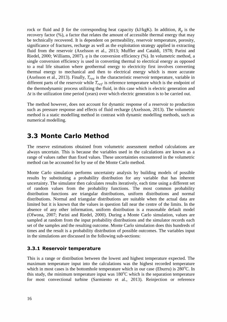
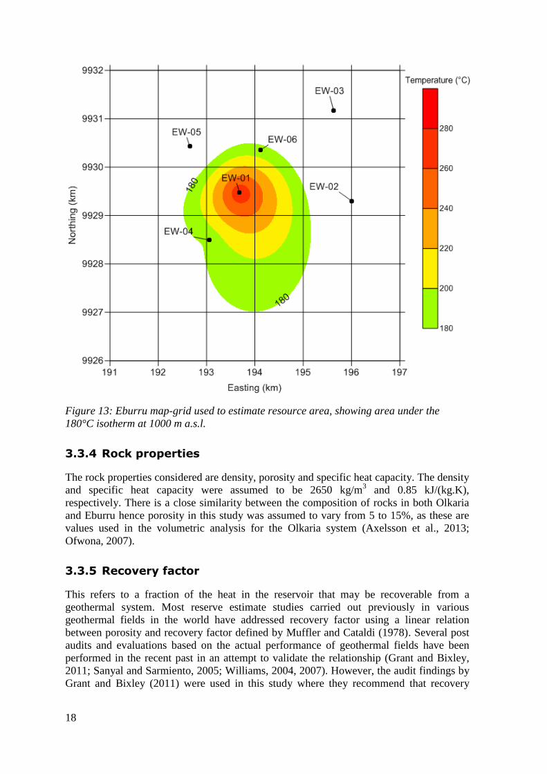
Figure 13: Eburru map-grid used to estimate resource area, showing area under the

180°C isotherm at 1000 m a.s.l. ....................................................................... 18

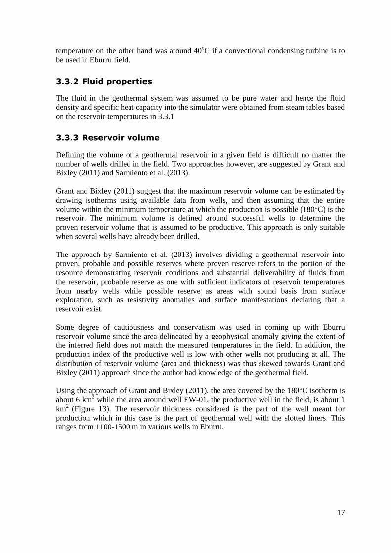
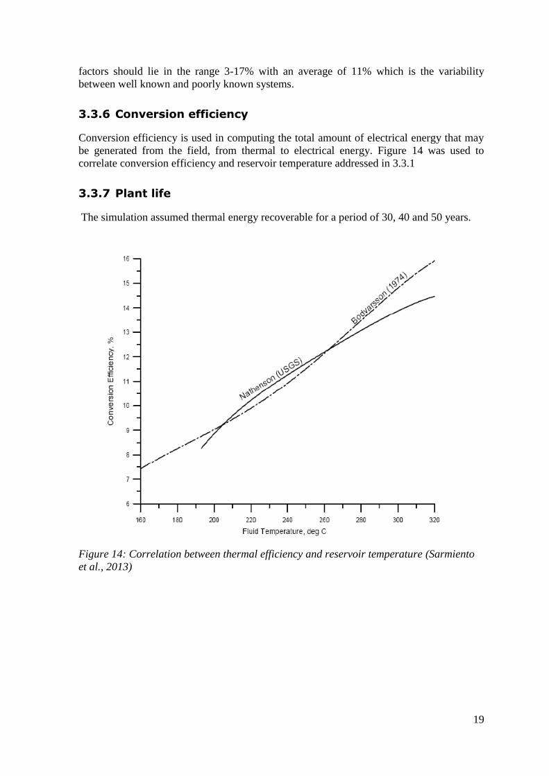
Figure 14: Correlation between thermal efficiency and reservoir temperature

(Sarmiento et al., 2013) .................................................................................... 19

Figure 15: Space discretization and the geometry data (Pruess, 1999). ............................ 23

Figure 16: Schematic of numerical modelling methodology............................................... 25

Figure 17: The numerical model grid of the Eburru geothermal system. ........................... 26

Figure 18: Vertical view of the model mesh for the Eburru geothermal system. ................ 27

Figure 19: Reservoir rocks clustered around the wells. ..................................................... 28

Figure 20: Average temperature per month for Eburru ..................................................... 29

x

Figure 21: T-S diagram of well EW-01. .............................................................................. 32

Figure 22: Production history of well EW-01 in Eburru. ................................................... 32

Figure 23: Location of hypothetical wells (red) in the Eburru geothermal field, used

for forecasting. ................................................................................................. 33

Figure 24: Comparison between observed and simulated temperatures. ........................... 35

Figure 25: Comparison between observed and simulated pressures. ................................ 35

Figure 26: Production history matching for EW-01. .......................................................... 36

Figure 27: Steam flow and the equivalent electric power for scenario I. ........................... 37

Figure 28: Pressure drawdown in layer K (100 m a.s.l) for scenario I. ............................. 38

Figure 29: Steam flow and the equivalent electric power for scenario II. ......................... 39

Figure 30: Pressure drawdown in layer K (100 m a.s.l) for scenario II. ........................... 39

xi

List of Tables

Table 1: Eburru geothermal field well information. ............................................................. 7

Table 2: Monte Carlo input data for the Eburru geothermal field. .................................... 20

Table 3: The results for the Monte Carlo volumetric assessment of the Eburru

geothermal system. ........................................................................................... 20

Table 4: Assumed physical properties for rocks in the numerical model of the Eburru

geothermal system. ........................................................................................... 28

xii

Nomenclature

A Area [m2]

D Distance [m]

E Thermal energy [J]

F Mass or heat flux [kg/s.m2] or [J/m

2s]

g Acceleration due to gravity [m/s2]

h Reservoir thickness [m] or enthalpy [J/kg]

k Absolute permeability [m2]

krβ Relative permeability [-]

M Mass per volume [kg/m3]

n Normal vector

P Pressure [Pa]

Pe Electric power [W]

q Mass flow rate [kg/s]

R Residual

Rg Recovery factor

S Saturation [m3/m

3]

T Temperature [°C]

t Time [s]

u Specific internal energy [J/kg]

U Darcy velocity [m/s]

V Volume [m3]

X Mass fraction

Greek letters

η Conversion efficiency

ρ Density [kg/m3]

μ Dynamic viscosity [kg/m.s]

ϕ Rock porosity

β Specific heat capacity [kJ/kg.K]

Γ Surface area [m2]

λ Thermal conductivity [W/m.°C]

xiii

Acknowledgements

My sincere gratitude to The Government of Iceland through the United Nations University

(UNU-GTP) and Kenya Electricity Generating Company (KenGen) for funding this MSc

study.

I would like to thank my supervisors Dr. Andri Arnaldsson, Dr. Gudni Axelsson and Dr.

Halldór Pálsson for their guidance and support throughout the project. I also extend my

thanks to Mr. Benedikt Steingrímsson for reviewing part of this work and to my fellow

colleague Mr. Vincent Koech for discussions and encouragement.

I appreciate the UNU-GTP staff for much assistance during my study and stay in Iceland.

Finally to my dear wife, Nkirote and to our sons, Kimathi and Koome, I salute you for your

patience, encouragements and support during the entire study period.

1

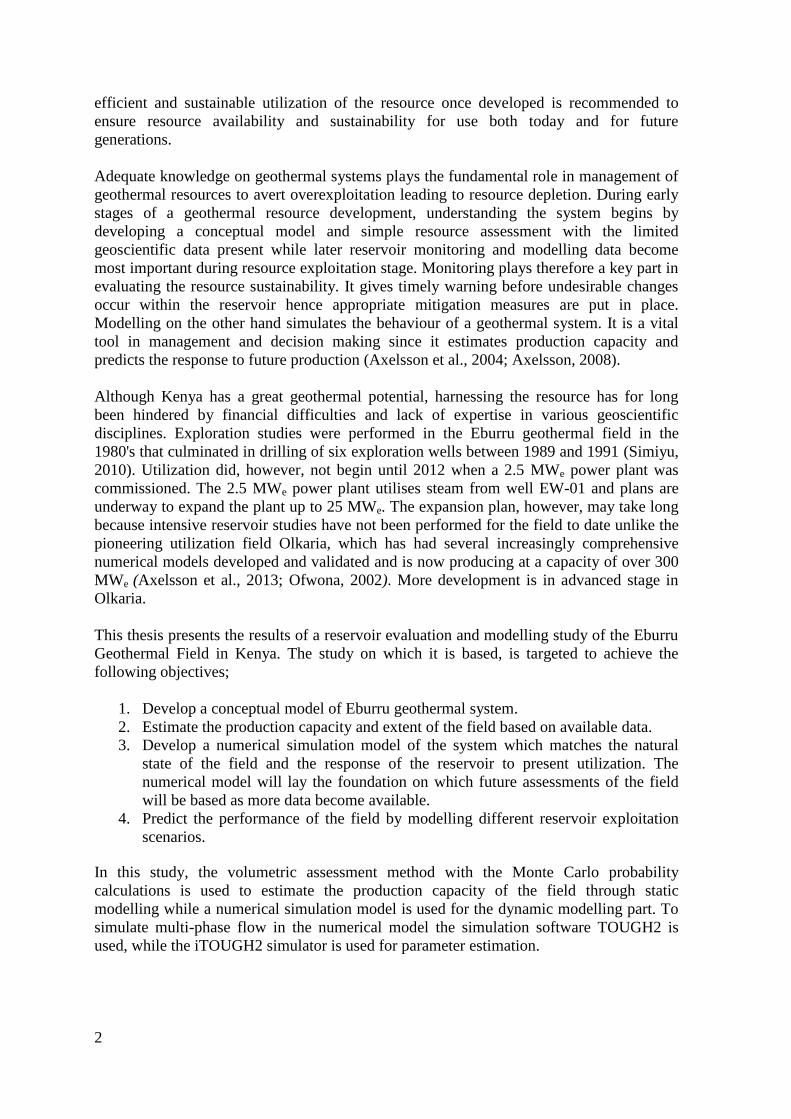
1 Introduction

Kenya has an installed generating capacity of 1,664 MWe of electricity against domestic

demand by a population of 40 million, institutions and industries. More than half of the

electricity supply is met by hydropower, mainly from the rivers Tana and Turkwel.

Demand for household energy (mainly from charcoal and wood) and demand for

agricultural land and timber production has put huge pressure on the country's forest cover

which is barely less than 3% of the total land (Mathu, 2011). This has severely affected the

catchment areas of the rivers utilised for hydropower generation, which consequently has

led to low water levels in the associated dams leaving consumers susceptible to power

outages and black-outs during dry seasons.

The demand-supply imbalance in the country has hitherto contributed to regular electricity

power rationing, particularly during dry spells. This undesirable situation has persisted

since 2006 and there is therefore a great need to correct it. To reduce rationing hours and

power outages, the government has put in temporary mitigation measures like connecting

thermal energy to the national grid. The thermal power plant installation cost is relatively

low but the cost of running the plants is high due to ever escalating oil prices. This then

increases the cost of electricity to prices unaffordable to most consumers. These power

outages coupled with high cost of electricity due to high oil prices has stagnated the

economic growth of the country in addition to raising the cost of living.

The government plans to fast track and develop the energy sector in line with Kenya vision

2030 policy, a policy to transform Kenya into a newly industrialised, middle-income

country by providing high quality life to all its citizens by 2030 in a clean and secure

environment. To achieve this goal, the government has embarked on generating reliable

electrical energy using other sources like coal, nuclear, wind and geothermal (Government

of the Republic of Kenya, 2007).

Geothermal energy is the immense natural heat of the earth, generated and stored in the

earth's core, mantle and crust. The natural heat is transferred from the interior towards the

surface mostly by conduction. This conductive heat flow, heats up the water of meteoric or

oceanic origin that percolates into the ground through faults and fissures. The heated water

rises through other faults and is replaced by more meteoric or oceanic water and hence

convective heat transfer is enhanced, creating geothermal systems. The potential of the

earth's geothermal resources is enormous when compared to its use today (Axelsson, 2013;

Fridleifsson et al., 2008). Geothermal energy is independent of the weather conditions and

thus can be used for both base load and peak power plants (Fridleifsson et al., 2008).

Geothermal resources are normally classified as renewable energy sources because they

are maintained by a continuous energy current. This is in accordance with the definition

that the energy extracted from the renewable sources is always replaced in a natural way

by additional amount of energy with the replacement taking place on a time-scale

comparable to that of the extracting rate (Axelsson, 2008). Even though the resources are

considered renewable, production capacity of geothermal resource is not unlimited thus

2

efficient and sustainable utilization of the resource once developed is recommended to

ensure resource availability and sustainability for use both today and for future

generations.

Adequate knowledge on geothermal systems plays the fundamental role in management of

geothermal resources to avert overexploitation leading to resource depletion. During early

stages of a geothermal resource development, understanding the system begins by

developing a conceptual model and simple resource assessment with the limited

geoscientific data present while later reservoir monitoring and modelling data become

most important during resource exploitation stage. Monitoring plays therefore a key part in

evaluating the resource sustainability. It gives timely warning before undesirable changes

occur within the reservoir hence appropriate mitigation measures are put in place.

Modelling on the other hand simulates the behaviour of a geothermal system. It is a vital

tool in management and decision making since it estimates production capacity and

predicts the response to future production (Axelsson et al., 2004; Axelsson, 2008).

Although Kenya has a great geothermal potential, harnessing the resource has for long

been hindered by financial difficulties and lack of expertise in various geoscientific

disciplines. Exploration studies were performed in the Eburru geothermal field in the

1980's that culminated in drilling of six exploration wells between 1989 and 1991 (Simiyu,

2010). Utilization did, however, not begin until 2012 when a 2.5 MWe power plant was

commissioned. The 2.5 MWe power plant utilises steam from well EW-01 and plans are

underway to expand the plant up to 25 MWe. The expansion plan, however, may take long

because intensive reservoir studies have not been performed for the field to date unlike the

pioneering utilization field Olkaria, which has had several increasingly comprehensive

numerical models developed and validated and is now producing at a capacity of over 300

MWe (Axelsson et al., 2013; Ofwona, 2002). More development is in advanced stage in

Olkaria.

This thesis presents the results of a reservoir evaluation and modelling study of the Eburru

Geothermal Field in Kenya. The study on which it is based, is targeted to achieve the

following objectives;

1. Develop a conceptual model of Eburru geothermal system.

2. Estimate the production capacity and extent of the field based on available data.

3. Develop a numerical simulation model of the system which matches the natural

state of the field and the response of the reservoir to present utilization. The

numerical model will lay the foundation on which future assessments of the field

will be based as more data become available.

4. Predict the performance of the field by modelling different reservoir exploitation

scenarios.

In this study, the volumetric assessment method with the Monte Carlo probability

calculations is used to estimate the production capacity of the field through static

modelling while a numerical simulation model is used for the dynamic modelling part. To

simulate multi-phase flow in the numerical model the simulation software TOUGH2 is

used, while the iTOUGH2 simulator is used for parameter estimation.

3

2 Eburru Geothermal Field

2.1 Background

Various geothermal surface manifestations such as fumaroles, geysers, hot grounds and hot

springs are eminent along the Kenyan rift. The rift, extending from Lake Turkana to Lake

Natron in northern Tanzania, is a part of The East African rift valley system that runs from

the Afar triple junction at the Gulf of Eden in the north to Mozambique in the south. It is

part of incipient continental diverging zone, a zone where thinning of the crust is occurring

and hence eruptions of lavas and associated volcanic activities (Lagat, 2003). A total of

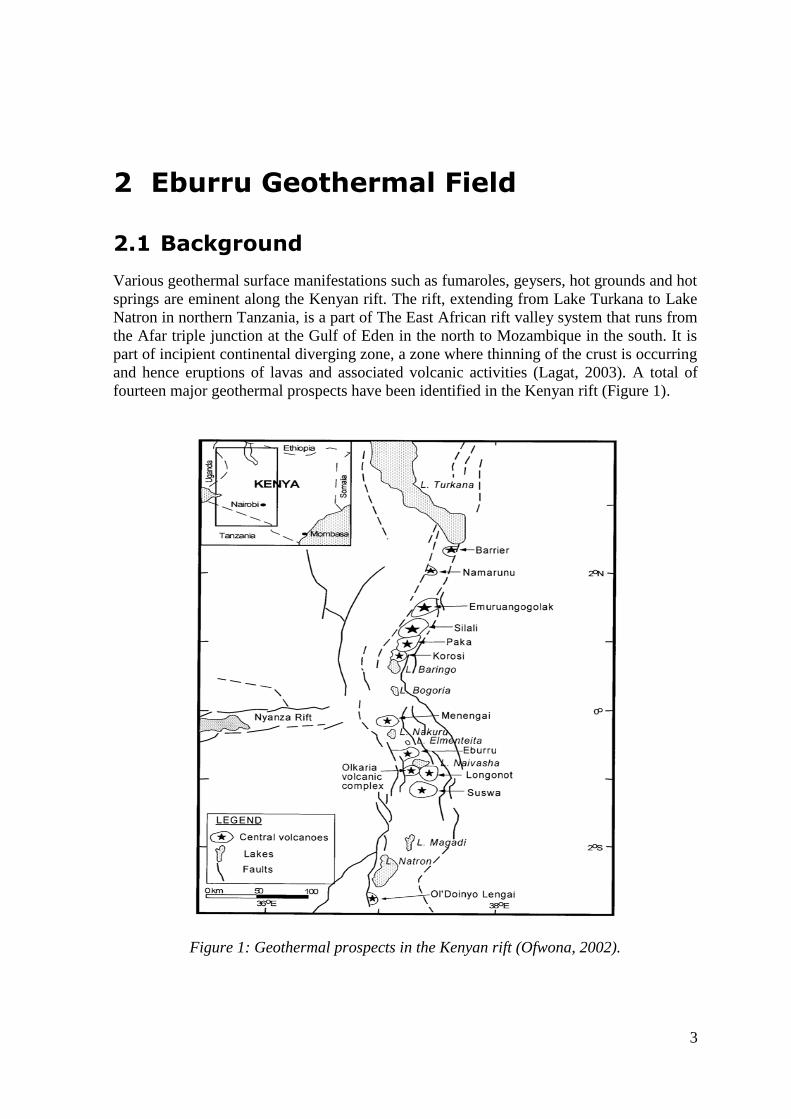
fourteen major geothermal prospects have been identified in the Kenyan rift (Figure 1).

Figure 1: Geothermal prospects in the Kenyan rift (Ofwona, 2002).

4

Only three prospects in the Kenyan rift have so far been drilled; Olkaria, Eburru and

Menengai. The Greater Olkaria geothermal field currently hosts three power plants and

three wellhead units. The Olkaria I and Olkaria II plants have a capacity of 45 MWe and

105 MWe respectively while the three wellhead units have a combined capacity of over 20

MWe. These two power plants together with the wellhead units are owned and operated by

Kenya Electricity Generating Company (KenGen). The Olkaria III with a capacity of 110

MWe, is owned and operated by an Independent Power Producer, OrPower4 Inc.

Construction of two more power plants with two 70 MWe turbines each (280 MWe in total)

is at an advanced stage with commissioning scheduled in mid-2014. This will bring the

power generated in this geothermal field to over 500 MWe. In addition, several wellhead

power plants are being put up to allow early generation as the company sources for more

funds to construct a big power plant (Axelsson et al., 2013; Market Watch – The Wall

street Journal, 2014; Thinkgeoenergy article, 2012).

Drilling of exploration wells in Menengai is currently in progress. The Geothermal

Development Company (GDC) has so far drilled over twenty wells in this field and plans

for a power plant ranging from 50-100 MWe are underway.

Eburru is located north of the Greater Olkaria geothermal field. The two fields are about

40km apart. Surface manifestations evident in the field include fumaroles, hot and

thermally altered grounds. Deep drilling of six wells to an average depth of 2500 m was

done between 1989 and 1991. Of the six wells drilled, only EW-01, EW-04 and EW-06

were productive, with an estimated capacity of 2.4 MWe, 1.0 MWe and 2.9 MWt

respectively, while the rest of the wells could not discharge (Lagat, 2003; Omenda, 2013).

The Eburru geothermal power plant, utilizing steam from well EW-01, has been generating

2.5 MWe since 2012 when the plant was commissioned. There are plans by KenGen to drill

and develop the field further.

2.2 Geological information

The Eburru volcano forms the highest topography within the entire Kenyan rift at an

elevation of about 2800 m. The volcano consists of east and west volcanic centres which

are composed of pyroclastics, rhyolites, basalts, trachytes, tuffs and pumice (Lagat, 2003).

The two volcanic centres are arranged in an E-W trend and extend as far to the west as the

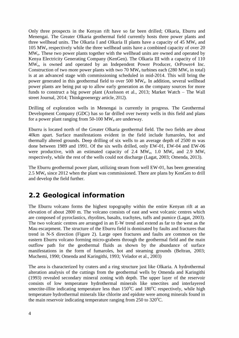
Mau escarpment. The structure of the Eburru field is dominated by faults and fractures that

trend in N-S direction (Figure 2). Large open fractures and faults are common on the

eastern Eburru volcano forming micro-grabens through the geothermal field and the main

outflow path for the geothermal fluids as shown by the abundance of surface

manifestations in the form of fumaroles, hot and steaming grounds (Beltran, 2003;

Muchemi, 1990; Omenda and Karingithi, 1993; Velador et al., 2003)

The area is characterized by craters and a ring structure just like Olkaria. A hydrothermal

alteration analysis of the cuttings from the geothermal wells by Omenda and Karingithi

(1993) revealed secondary mineral zoning with depth. The upper layer of the reservoir

consists of low temperature hydrothermal minerals like smectites and interlayered

smectite-illite indicating temperature less than 150oC and 180

oC respectively, while high

temperature hydrothermal minerals like chlorite and epidote were among minerals found in

the main reservoir indicating temperature ranging from 250 to 320oC.

5

The hydrothermal alteration minerals, however, indicate that the geothermal system is

cooling at present. Apart from well EW-01, the minerals indicate high temperatures but

compared to the measured temperatures there is a temperature drop at the boundary of the

field by more than 130°C in wells EW-02 and EW-05, 150°C in well EW-03, 80°C in well

EW-04 and 40°C in well EW-06. This shows that the heat source is cooling, allowing

incursions of cold ground water into the reservoir.

Figure 2: A geological map of Eburru showing the main geological structures (Omenda

and Karingithi, 1993).

2.3 Geophysical exploration

Various geophysical methods have been used to image the Eburru geothermal system. In

the early stages of exploration, gravity and Schlumberger resistivity methods were used

while MT and TEM resistivity surveying have been applied in recent work.

Gravity surveys of the East African rift system show a progressive change from north to

south in accordance with crustal separation and magmatic intensity. In the Red Sea where

crustal separation is significant and dense materials have intruded upwards, the gravity

anomalies are highest. Ethiopia has a positive anomaly while in Kenya there is a narrow

6

positive anomaly within a broader negative anomaly (-50 mgal) and the anomaly

disappears in North-Tanzania (Saemundsson, 2008). The Kenyan dome region is

characterised by a regional gravity low, with its maximum low in the Eburru and Olkaria

areas. However, within the general gravity low a localised high exists beneath the Eburru-

Olkaria volcanic complexes. The high density bodies underlying these complexes are

interpreted as mafic magma chambers (Velador et al., 2003).

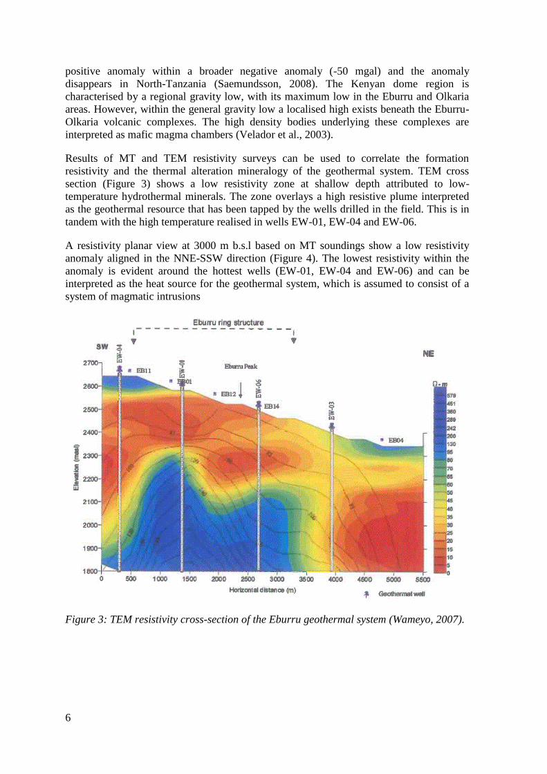
Results of MT and TEM resistivity surveys can be used to correlate the formation

resistivity and the thermal alteration mineralogy of the geothermal system. TEM cross

section (Figure 3) shows a low resistivity zone at shallow depth attributed to low-

temperature hydrothermal minerals. The zone overlays a high resistive plume interpreted

as the geothermal resource that has been tapped by the wells drilled in the field. This is in

tandem with the high temperature realised in wells EW-01, EW-04 and EW-06.

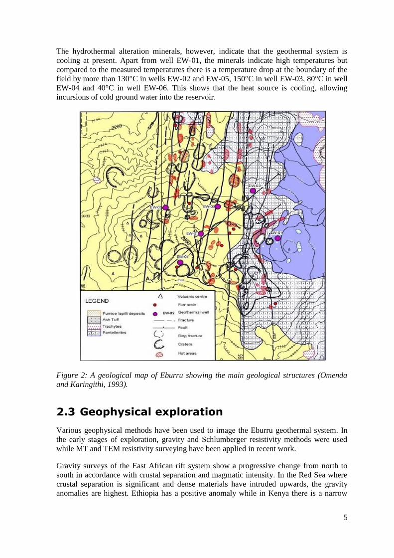
A resistivity planar view at 3000 m b.s.l based on MT soundings show a low resistivity

anomaly aligned in the NNE-SSW direction (Figure 4). The lowest resistivity within the

anomaly is evident around the hottest wells (EW-01, EW-04 and EW-06) and can be

interpreted as the heat source for the geothermal system, which is assumed to consist of a

system of magmatic intrusions

Figure 3: TEM resistivity cross-section of the Eburru geothermal system (Wameyo, 2007).

7

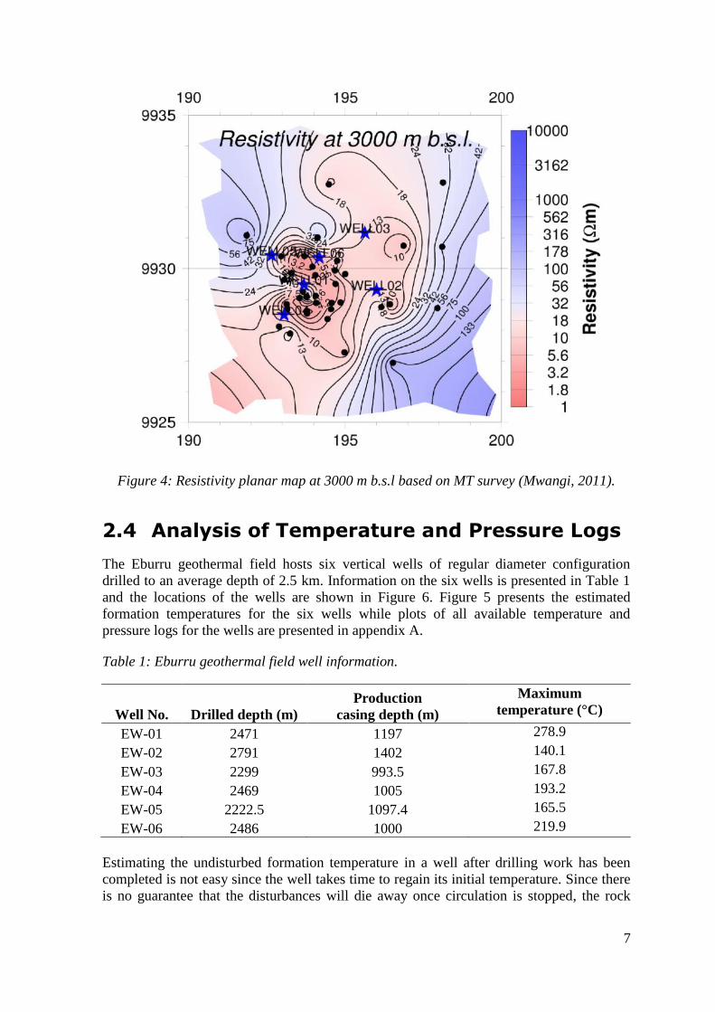
Figure 4: Resistivity planar map at 3000 m b.s.l based on MT survey (Mwangi, 2011).

2.4 Analysis of Temperature and Pressure Logs

The Eburru geothermal field hosts six vertical wells of regular diameter configuration

drilled to an average depth of 2.5 km. Information on the six wells is presented in Table 1

and the locations of the wells are shown in Figure 6. Figure 5 presents the estimated

formation temperatures for the six wells while plots of all available temperature and

pressure logs for the wells are presented in appendix A.

Table 1: Eburru geothermal field well information.

Well No. Drilled depth (m)

Production

casing depth (m)

Maximum

temperature (°C)

EW-01 2471 1197 278.9

EW-02 2791 1402 140.1

EW-03 2299 993.5 167.8

EW-04 2469 1005 193.2

EW-05 2222.5 1097.4 165.5

EW-06 2486 1000 219.9

Estimating the undisturbed formation temperature in a well after drilling work has been

completed is not easy since the well takes time to regain its initial temperature. Since there

is no guarantee that the disturbances will die away once circulation is stopped, the rock

8

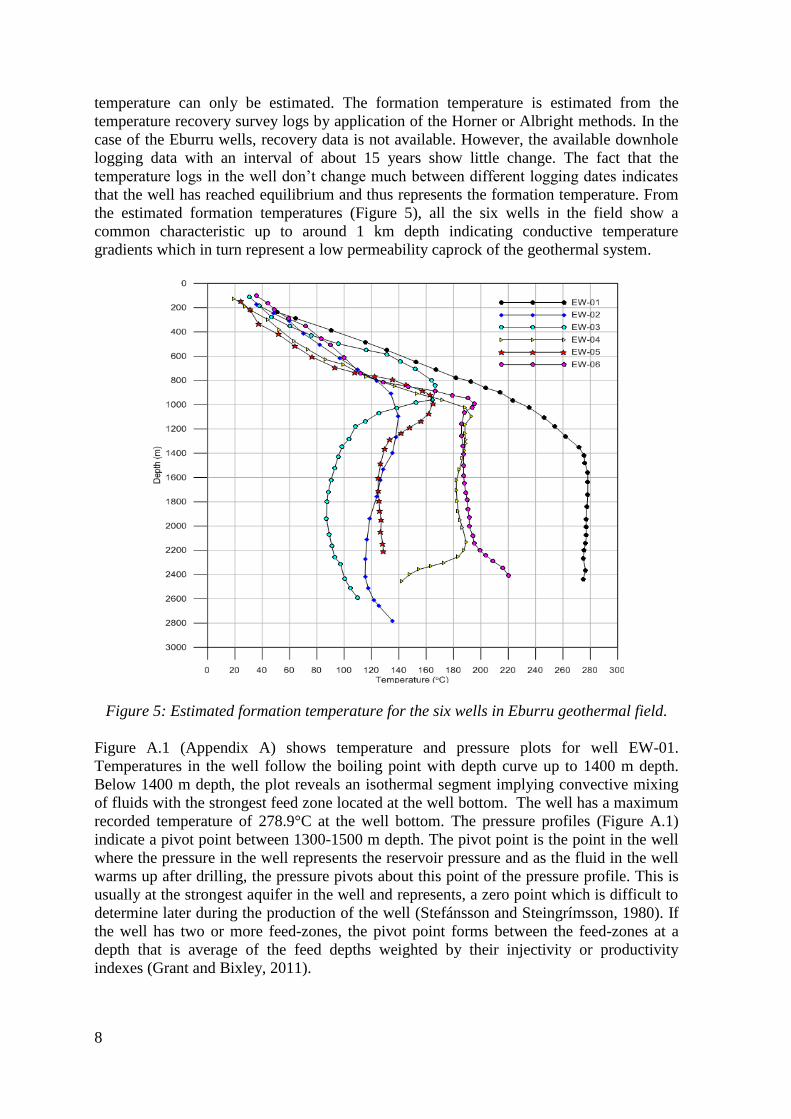
temperature can only be estimated. The formation temperature is estimated from the

temperature recovery survey logs by application of the Horner or Albright methods. In the

case of the Eburru wells, recovery data is not available. However, the available downhole

logging data with an interval of about 15 years show little change. The fact that the

temperature logs in the well don’t change much between different logging dates indicates

that the well has reached equilibrium and thus represents the formation temperature. From

the estimated formation temperatures (Figure 5), all the six wells in the field show a

common characteristic up to around 1 km depth indicating conductive temperature

gradients which in turn represent a low permeability caprock of the geothermal system.

Figure 5: Estimated formation temperature for the six wells in Eburru geothermal field.

Figure A.1 (Appendix A) shows temperature and pressure plots for well EW-01.

Temperatures in the well follow the boiling point with depth curve up to 1400 m depth.

Below 1400 m depth, the plot reveals an isothermal segment implying convective mixing

of fluids with the strongest feed zone located at the well bottom. The well has a maximum

recorded temperature of 278.9°C at the well bottom. The pressure profiles (Figure A.1)

indicate a pivot point between 1300-1500 m depth. The pivot point is the point in the well

where the pressure in the well represents the reservoir pressure and as the fluid in the well

warms up after drilling, the pressure pivots about this point of the pressure profile. This is

usually at the strongest aquifer in the well and represents, a zero point which is difficult to

determine later during the production of the well (Stefánsson and Steingrímsson, 1980). If

the well has two or more feed-zones, the pivot point forms between the feed-zones at a

depth that is average of the feed depths weighted by their injectivity or productivity

indexes (Grant and Bixley, 2011).

9

Figures A.2, A.3 and A.5 show temperature and pressure plots for wells EW-02, EW-03

and EW-05, respectively. The three well plots show relatively low temperatures with

inversion at depth implying a possible flow of cold water into the reservoir and that they

may lay at the outer boundary of the system. It is worth noting that the wells are very far

from boiling conditions. These wells did not discharge at all even after several airlifting

attempts. The pressure plots (Figure A.2, A.3 and A.5) available are not enough to

determine the pivot points in the wells.

An isothermal segment implying convective mixing of fluids is present in both of wells

EW-04 and EW-06 (Figures 5, A.4 and A.6). Both wells appear to have a major feed-zone

at around 2200 m depth. Below this depth, an inversion is observed in EW-04 indicating

that the well penetrates through the reservoir. On the other hand, EW-06 exhibits

completely different characteristic and positive temperature gradient below 2200 m depth.

The temperature profile shows heat transfer by conduction suggesting a relatively

impermeable formation below 2200 m and possibly proximity to upflow and heat source

for the reservoir.

The Eburru geothermal system is classified as liquid dominated. Liquid dominated

geothermal reservoirs have water temperature at or below the boiling point at the

prevailing pressures and the liquid water phase controls the pressure in the reservoir

(Axelsson, 2008). On the basis of temperature classification, Eburru has a high-

temperature system within the caldera region where reservoir temperatures exceed 200°C

at 1 km depth. Outside the caldera, the subsurface temperature are much lower and

possible geothermal resources there fall under the classification as low-temperature

systems as temperatures at 1 km depth are well below 150°C.

One way to visualise downhole data is by plotting planar views or cross sections hence

producing isovalue maps which represents the most basic aspects of a geothermal

reservoir. These isovalue maps can be produced using temperature and pressure data but

temperature is probably the most important parameter to analyse the geothermal reservoir

when sufficient wells have been drilled. Temperatures outside the reservoir are as

important as those within and should be included. These peripheral temperatures help

define the field boundaries which are important in the numerical simulations since they

imply permeability or its absence (Grant and Bixley, 2011).

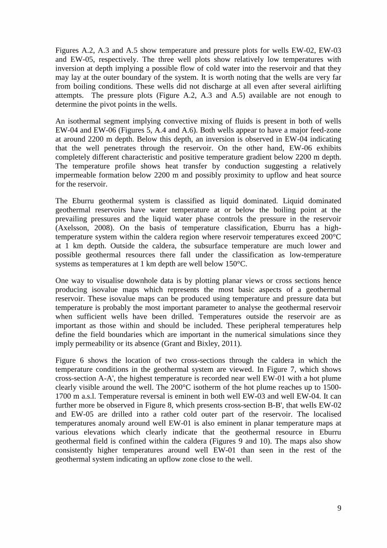
Figure 6 shows the location of two cross-sections through the caldera in which the

temperature conditions in the geothermal system are viewed. In Figure 7, which shows

cross-section A-A', the highest temperature is recorded near well EW-01 with a hot plume

clearly visible around the well. The 200°C isotherm of the hot plume reaches up to 1500-

1700 m a.s.l. Temperature reversal is eminent in both well EW-03 and well EW-04. It can

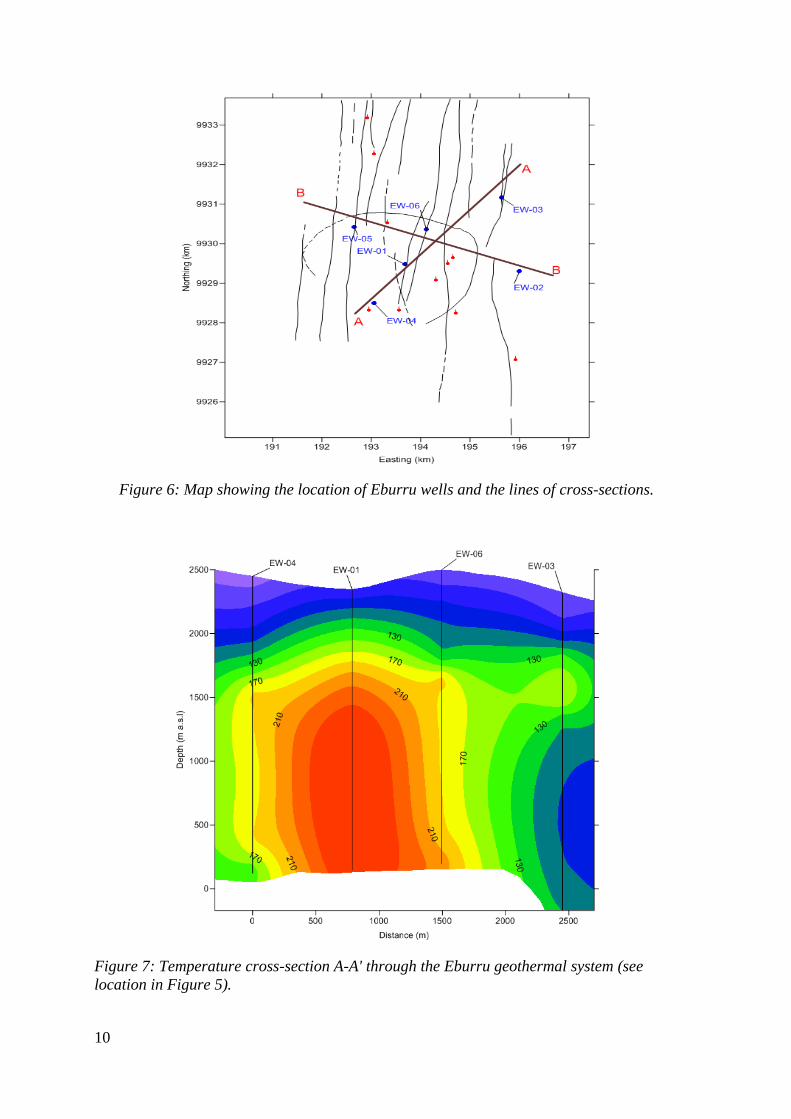
further more be observed in Figure 8, which presents cross-section B-B', that wells EW-02

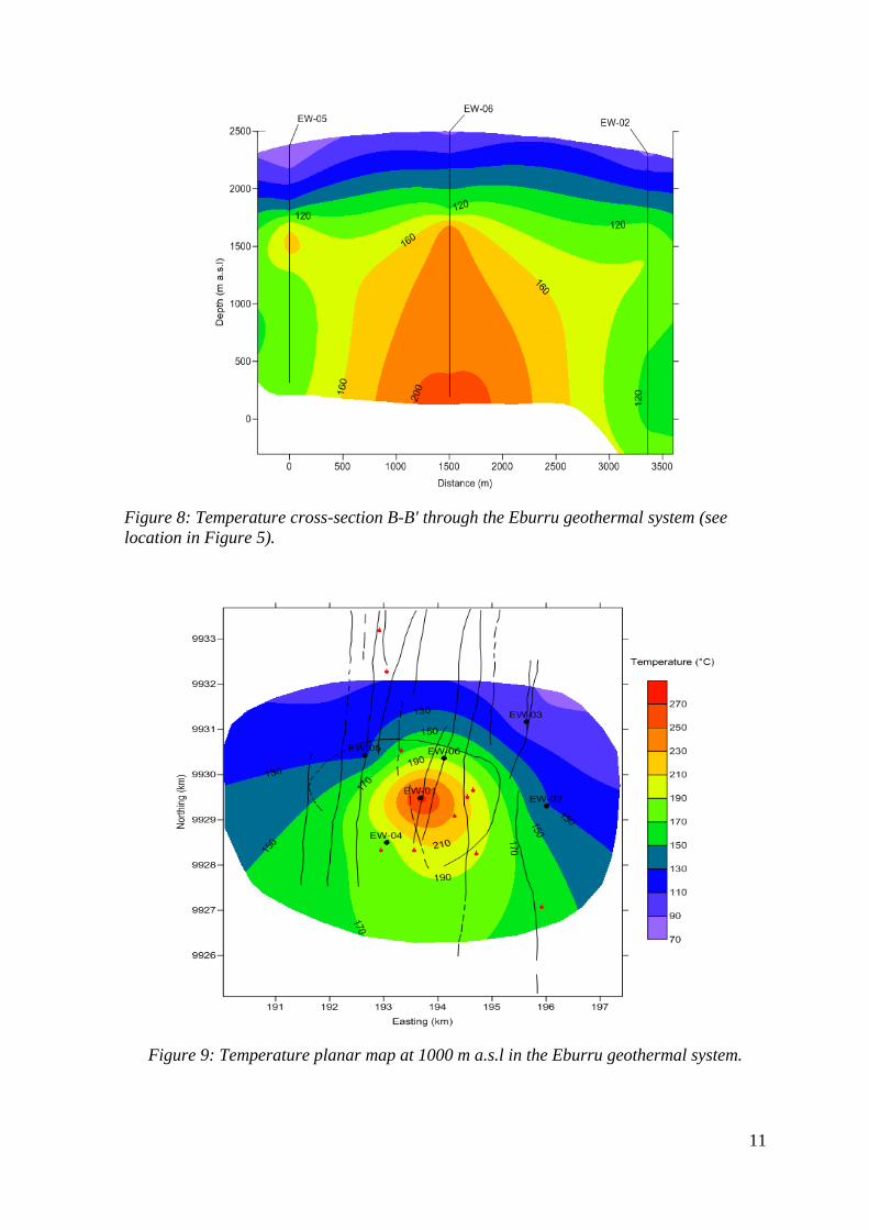
and EW-05 are drilled into a rather cold outer part of the reservoir. The localised

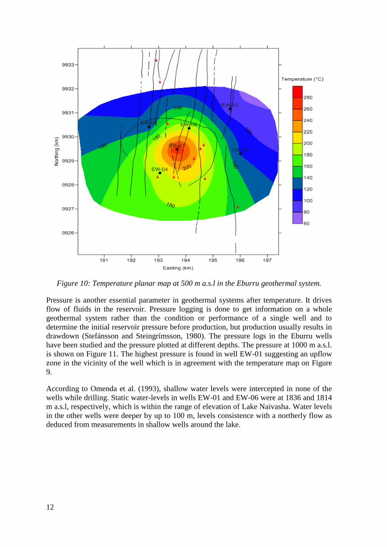
temperatures anomaly around well EW-01 is also eminent in planar temperature maps at

various elevations which clearly indicate that the geothermal resource in Eburru

geothermal field is confined within the caldera (Figures 9 and 10). The maps also show

consistently higher temperatures around well EW-01 than seen in the rest of the

geothermal system indicating an upflow zone close to the well.

10

Figure 6: Map showing the location of Eburru wells and the lines of cross-sections.

Figure 7: Temperature cross-section A-A' through the Eburru geothermal system (see

location in Figure 5).

11

Figure 8: Temperature cross-section B-B' through the Eburru geothermal system (see

location in Figure 5).

Figure 9: Temperature planar map at 1000 m a.s.l in the Eburru geothermal system.

12

Figure 10: Temperature planar map at 500 m a.s.l in the Eburru geothermal system.

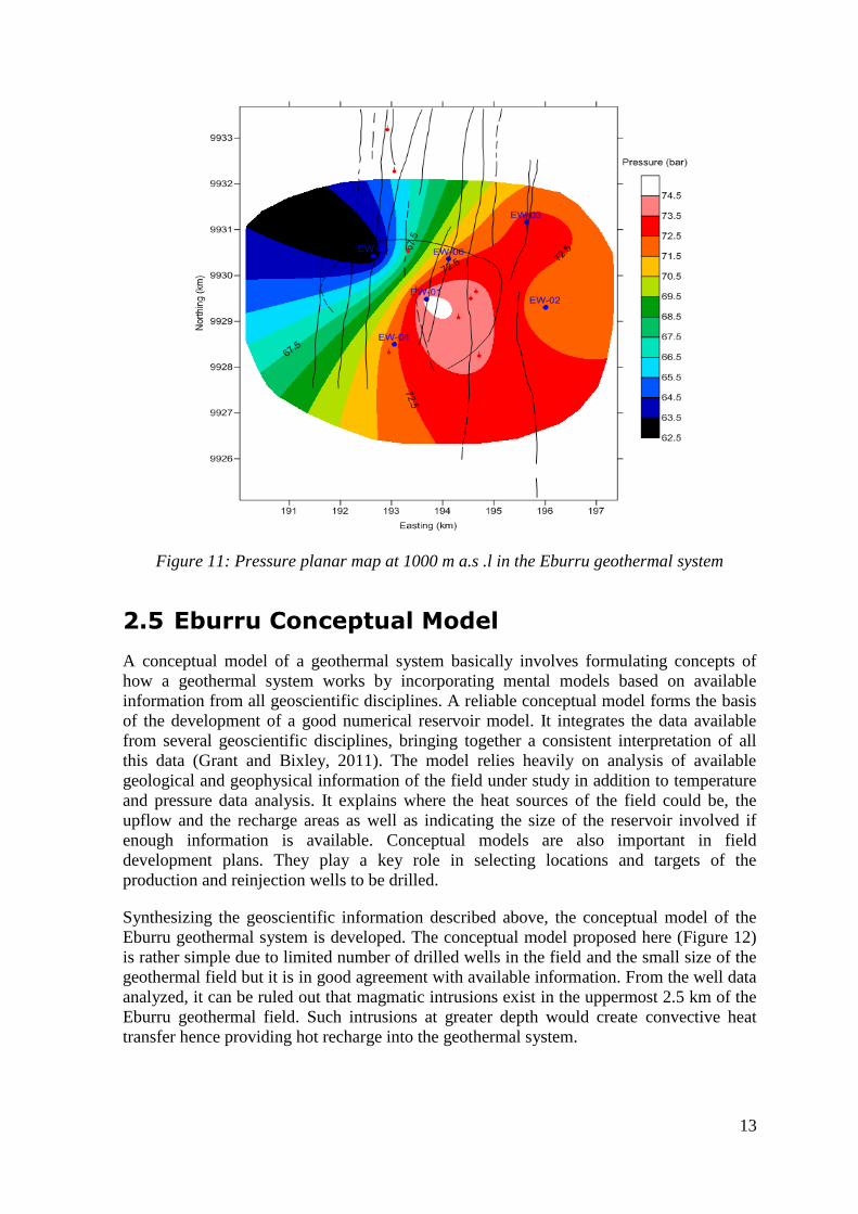
Pressure is another essential parameter in geothermal systems after temperature. It drives

flow of fluids in the reservoir. Pressure logging is done to get information on a whole

geothermal system rather than the condition or performance of a single well and to

determine the initial reservoir pressure before production, but production usually results in

drawdown (Stefánsson and Steingrímsson, 1980). The pressure logs in the Eburru wells

have been studied and the pressure plotted at different depths. The pressure at 1000 m a.s.l.

is shown on Figure 11. The highest pressure is found in well EW-01 suggesting an upflow

zone in the vicinity of the well which is in agreement with the temperature map on Figure

9.

According to Omenda et al. (1993), shallow water levels were intercepted in none of the

wells while drilling. Static water-levels in wells EW-01 and EW-06 were at 1836 and 1814

m a.s.l, respectively, which is within the range of elevation of Lake Naivasha. Water levels

in the other wells were deeper by up to 100 m, levels consistence with a northerly flow as

deduced from measurements in shallow wells around the lake.

13

Figure 11: Pressure planar map at 1000 m a.s .l in the Eburru geothermal system

2.5 Eburru Conceptual Model

A conceptual model of a geothermal system basically involves formulating concepts of

how a geothermal system works by incorporating mental models based on available

information from all geoscientific disciplines. A reliable conceptual model forms the basis

of the development of a good numerical reservoir model. It integrates the data available

from several geoscientific disciplines, bringing together a consistent interpretation of all

this data (Grant and Bixley, 2011). The model relies heavily on analysis of available

geological and geophysical information of the field under study in addition to temperature

and pressure data analysis. It explains where the heat sources of the field could be, the

upflow and the recharge areas as well as indicating the size of the reservoir involved if

enough information is available. Conceptual models are also important in field

development plans. They play a key role in selecting locations and targets of the

production and reinjection wells to be drilled.

Synthesizing the geoscientific information described above, the conceptual model of the

Eburru geothermal system is developed. The conceptual model proposed here (Figure 12)

is rather simple due to limited number of drilled wells in the field and the small size of the

geothermal field but it is in good agreement with available information. From the well data

analyzed, it can be ruled out that magmatic intrusions exist in the uppermost 2.5 km of the

Eburru geothermal field. Such intrusions at greater depth would create convective heat

transfer hence providing hot recharge into the geothermal system.

14

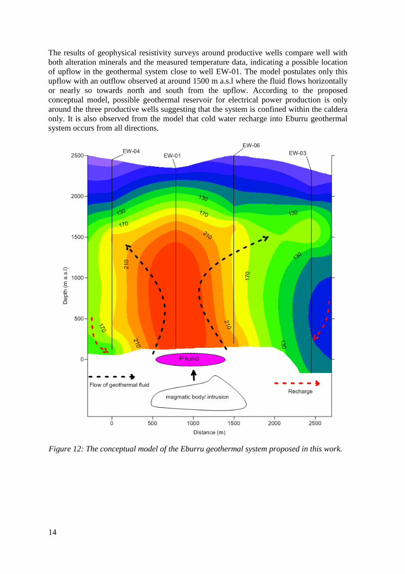
The results of geophysical resistivity surveys around productive wells compare well with

both alteration minerals and the measured temperature data, indicating a possible location

of upflow in the geothermal system close to well EW-01. The model postulates only this

upflow with an outflow observed at around 1500 m a.s.l where the fluid flows horizontally

or nearly so towards north and south from the upflow. According to the proposed

conceptual model, possible geothermal reservoir for electrical power production is only

around the three productive wells suggesting that the system is confined within the caldera

only. It is also observed from the model that cold water recharge into Eburru geothermal

system occurs from all directions.

Figure 12: The conceptual model of the Eburru geothermal system proposed in this work.

15

3 Reserve Estimation

3.1 Introduction

The primary reason for gathering geological, geophysical, geochemical and downhole data

is to be able to estimate the generating potential of the geothermal resource being

considered (Bodvarsson et al., 1989). Reserve estimation is used mostly in early stages of

geothermal field development since it neither requires significant number of wells nor a

long production history, as is the case with numerical modelling. There are various

methods available for estimating the potential of a geothermal system at an early stage of

development, but all have shortcomings in determining the amount of hot fluids in place,

rate of natural fluid recharge to the reservoir, the rate at which these fluids can be

economically extracted and the best program to develop the field at this early stage. The

most common method for estimating the potential of a geothermal system is the so-called

volumetric method applied together with Monte Carlo calculations. These two methods are

described below.

3.2 Volumetric Assessment Method

The volumetric method is one of the basic methods of assessing the potential of a

geothermal field in its preliminary stage of development. It is mostly applied to justify

drilling and commitment for a specified power plant. The method involves estimating the

amount of thermal energy stored in a reservoir, both in the rock matrix and the fluid

entrapped in the pores. It assumes that the reservoir rocks are porous and permeable and

that the water mass extracted from the reservoir extracts the heat from the whole volume of

the reservoir.

According to Williams (2007), the electric power generation potential from a geothermal

system depends on the thermal energy present in the reservoir, the amount of thermal

energy that can be extracted at wellhead and the thermal efficiency with which that

wellhead thermal energy can be converted to electric power. The total thermal energy

contained in a reservoir is estimated as;

(3.1)

While electric power recoverable from the reservoir is given by the equation;

(3.2)

In the equation 3.1 and 3.2, V (= Ah: area and thickness) stands for the reservoir volume

under the study (m3), ϕ for the porosity of the rock (%), ρ for the density (kg/m

3) of the

16

rock or fluid and β for the corresponding heat capacity (kJ/kgK). In addition, Rg is the

recovery factor (%), a factor that relates the amount of accessible thermal energy that may

be technically recovered. It is dependent on permeability, reservoir temperature, porosity,

significance of fractures, recharge as well as the exploitation strategy applied in extracting

fluid from the reservoir (Axelsson et al., 2013; Muffler and Cataldi, 1978; Parini and

Riedel, 2000; Williams, 2007). η is the conversion efficiency (%). In volumetric method, a

single conversion efficiency is used in converting thermal to electrical energy as opposed

to a real life situation where geothermal energy to electricity first involves converting

thermal energy to mechanical and then to electrical energy which is more accurate

(Axelsson et al., 2013). Finally, is the characteristic reservoir temperature, variable in

different parts of the reservoir while is reference temperature which is the endpoint of

the thermodynamic process utilizing the fluid, in this case which is electric generation and

Δt is the utilization time period (years) over which electric generation is to be carried out.

The method however, does not account for dynamic response of a reservoir to production

such as pressure response and effects of fluid recharge (Axelsson, 2013). The volumetric

method is a static modelling method in contrast with dynamic modelling methods, such as

numerical modelling.

3.3 Monte Carlo Method

The reserve estimations obtained from volumetric assessment method calculations are

always uncertain. This is because the variables used in the calculations are known as a

range of values rather than fixed values. These uncertainties encountered in the volumetric

method can be accounted for by use of the Monte Carlo method.

Monte Carlo simulation performs uncertainty analysis by building models of possible

results by substituting a probability distribution for any variable that has inherent

uncertainty. The simulator then calculates results iteratively, each time using a different set

of random values from the probability functions. The most common probability

distribution functions are triangular distributions, uniform distributions and normal

distributions. Normal and triangular distributions are suitable when the actual data are

limited but it is known that the values in question fall near the centre of the limits. In the

absence of any other information, uniform distribution is a reasonable default model

(Ofwona, 2007; Parini and Riedel, 2000). During a Monte Carlo simulation, values are

sampled at random from the input probability distributions and the simulator records each

set of the samples and the resulting outcome. Monte Carlo simulation does this hundreds of

times and the result is a probability distribution of possible outcomes. The variables input

in the simulations are discussed in the following sub-sections:

3.3.1 Reservoir temperature

This is a range or distribution between the lowest and highest temperature expected. The

maximum temperature input into the calculations was the highest recorded temperature

which in most cases is the bottomhole temperature which in our case (Eburru) is 280oC. In

this study, the minimum temperature input was 180oC which is the separation temperature

for most convectional turbine (Sarmiento et al., 2013). Reinjection or reference

17

temperature on the other hand was around 40oC if a convectional condensing turbine is to

be used in Eburru field.

3.3.2 Fluid properties

The fluid in the geothermal system was assumed to be pure water and hence the fluid

density and specific heat capacity into the simulator were obtained from steam tables based

on the reservoir temperatures in 3.3.1

3.3.3 Reservoir volume

Defining the volume of a geothermal reservoir in a given field is difficult no matter the

number of wells drilled in the field. Two approaches however, are suggested by Grant and

Bixley (2011) and Sarmiento et al. (2013).

Grant and Bixley (2011) suggest that the maximum reservoir volume can be estimated by

drawing isotherms using available data from wells, and then assuming that the entire

volume within the minimum temperature at which the production is possible (180°C) is the

reservoir. The minimum volume is defined around successful wells to determine the

proven reservoir volume that is assumed to be productive. This approach is only suitable

when several wells have already been drilled.

The approach by Sarmiento et al. (2013) involves dividing a geothermal reservoir into

proven, probable and possible reserves where proven reserve refers to the portion of the

resource demonstrating reservoir conditions and substantial deliverability of fluids from

the reservoir, probable reserve as one with sufficient indicators of reservoir temperatures

from nearby wells while possible reserve as areas with sound basis from surface

exploration, such as resistivity anomalies and surface manifestations declaring that a

reservoir exist.

Some degree of cautiousness and conservatism was used in coming up with Eburru

reservoir volume since the area delineated by a geophysical anomaly giving the extent of

the inferred field does not match the measured temperatures in the field. In addition, the

production index of the productive well is low with other wells not producing at all. The

distribution of reservoir volume (area and thickness) was thus skewed towards Grant and

Bixley (2011) approach since the author had knowledge of the geothermal field.

Using the approach of Grant and Bixley (2011), the area covered by the 180°C isotherm is

about 6 km2 while the area around well EW-01, the productive well in the field, is about 1

km2

(Figure 13). The reservoir thickness considered is the part of the well meant for

production which in this case is the part of geothermal well with the slotted liners. This

ranges from 1100-1500 m in various wells in Eburru.

18

Figure 13: Eburru map-grid used to estimate resource area, showing area under the

180°C isotherm at 1000 m a.s.l.

3.3.4 Rock properties

The rock properties considered are density, porosity and specific heat capacity. The density

and specific heat capacity were assumed to be 2650 kg/m3 and 0.85 kJ/(kg.K),

respectively. There is a close similarity between the composition of rocks in both Olkaria

and Eburru hence porosity in this study was assumed to vary from 5 to 15%, as these are

values used in the volumetric analysis for the Olkaria system (Axelsson et al., 2013;

Ofwona, 2007).

3.3.5 Recovery factor

This refers to a fraction of the heat in the reservoir that may be recoverable from a

geothermal system. Most reserve estimate studies carried out previously in various

geothermal fields in the world have addressed recovery factor using a linear relation

between porosity and recovery factor defined by Muffler and Cataldi (1978). Several post

audits and evaluations based on the actual performance of geothermal fields have been

performed in the recent past in an attempt to validate the relationship (Grant and Bixley,

2011; Sanyal and Sarmiento, 2005; Williams, 2004, 2007). However, the audit findings by

Grant and Bixley (2011) were used in this study where they recommend that recovery

19

factors should lie in the range 3-17% with an average of 11% which is the variability

between well known and poorly known systems.

3.3.6 Conversion efficiency

Conversion efficiency is used in computing the total amount of electrical energy that may

be generated from the field, from thermal to electrical energy. Figure 14 was used to

correlate conversion efficiency and reservoir temperature addressed in 3.3.1

3.3.7 Plant life

The simulation assumed thermal energy recoverable for a period of 30, 40 and 50 years.

Figure 14: Correlation between thermal efficiency and reservoir temperature (Sarmiento

et al., 2013)

20

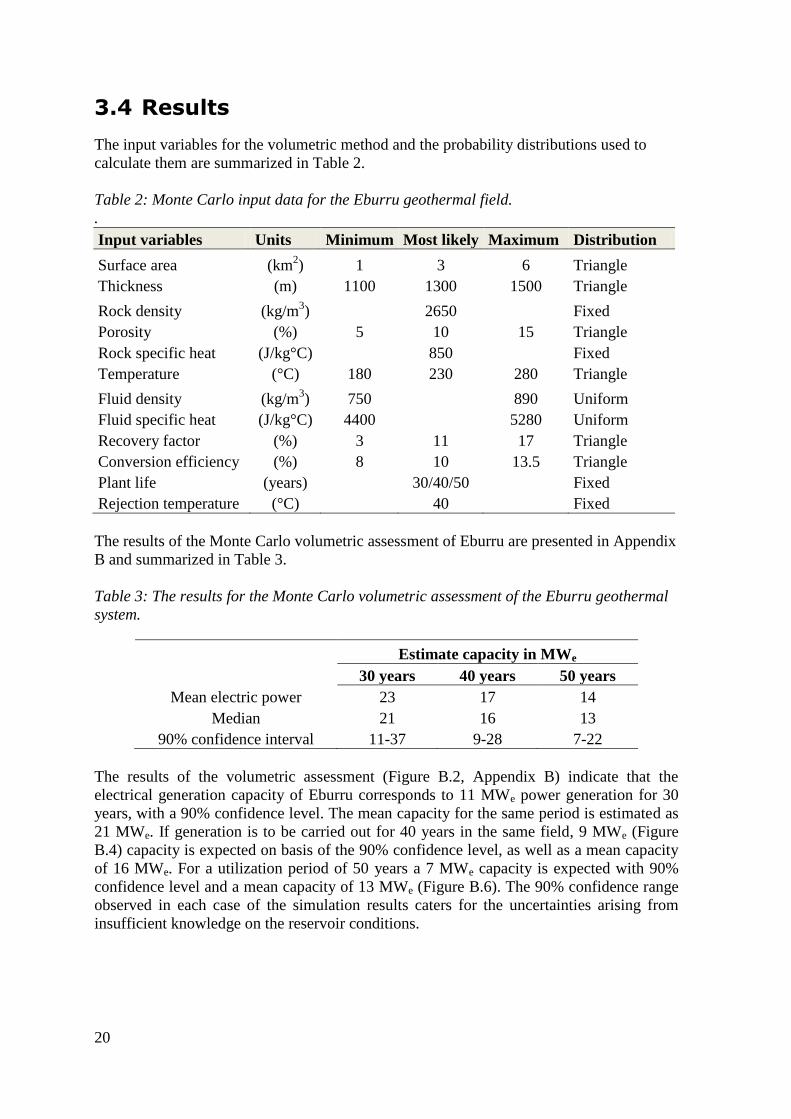
3.4 Results

The input variables for the volumetric method and the probability distributions used to

calculate them are summarized in Table 2.

Table 2: Monte Carlo input data for the Eburru geothermal field.

.

Input variables Units Minimum Most likely Maximum Distribution

Surface area (km2) 1 3 6 Triangle

Thickness (m) 1100 1300 1500 Triangle

Rock density (kg/m3)

2650

Fixed

Porosity (%) 5 10 15 Triangle

Rock specific heat (J/kg°C)

850

Fixed

Temperature (°C) 180 230 280 Triangle

Fluid density (kg/m3) 750

890 Uniform

Fluid specific heat (J/kg°C) 4400

5280 Uniform

Recovery factor (%) 3 11 17 Triangle

Conversion efficiency (%) 8 10 13.5 Triangle

Plant life (years)

30/40/50

Fixed

Rejection temperature (°C) 40 Fixed

The results of the Monte Carlo volumetric assessment of Eburru are presented in Appendix

B and summarized in Table 3.

Table 3: The results for the Monte Carlo volumetric assessment of the Eburru geothermal

system.

Estimate capacity in MWe

30 years 40 years 50 years

Mean electric power 23 17 14

Median 21 16 13

90% confidence interval 11-37 9-28 7-22

The results of the volumetric assessment (Figure B.2, Appendix B) indicate that the

electrical generation capacity of Eburru corresponds to 11 MWe power generation for 30

years, with a 90% confidence level. The mean capacity for the same period is estimated as

21 MWe. If generation is to be carried out for 40 years in the same field, 9 MWe (Figure

B.4) capacity is expected on basis of the 90% confidence level, as well as a mean capacity

of 16 MWe. For a utilization period of 50 years a 7 MWe capacity is expected with 90%

confidence level and a mean capacity of 13 MWe (Figure B.6). The 90% confidence range

observed in each case of the simulation results caters for the uncertainties arising from

insufficient knowledge on the reservoir conditions.

21

4 Theoretical Background of Numerical Modelling

4.1 Forward Model

TOUGH2 is a general purpose numerical simulator for non-isothermal flow of multi-

component, multi-phase fluids in one, two or three dimensional porous and fractured media

(Pruess et al., 1999). The basic mass conservation equations governing this kind of flow

can be written in the form;

(4.1)

F denotes the mass flux, q denotes sinks and sources while .n is a normal vector on the

surface element , pointing inwards into and M is the mass per volume. Equation 4.1

expresses the fact that the rate of change of fluid mass in is equal to the net inflow

across the surface of plus net gain from the fluid sources.

The general form of the mass accumulation term is

(4.2)

In the equation above, the total mass of the component k is obtained by summing over the

fluid phases β (that is liquid, gases). is the porosity, is the saturation of the phase β,

is the density of phase β and is the mass fraction of component k present in phase β.

Similarly the heat accumulation in the multiphase system is

(4.3)

Where and are grain density and specific heat of the rock respectively, T is temperature and

is specific internal energy in phase β.

22

Advective mass flux is the sum over phases.

and individual phase flux is given by a multiple version of the Darcy's law:

(4.5)

is the Darcy velocity (volume flux) in phase β, k is absolute permeability, is the

relative permeability to phase β, is the viscosity while is the fluid pressure in phase β

normally obtained by summing the pressure of a reference gas phase and the capillary

pressure.

Heat flux includes conductive and convective components

(4.6)

Where λ is thermal conductivity and is the specific enthalpy in phase β.

4.1.1 Space and time discretization

For numerical simulations, the continuous space and time must be discretized. The mass

and energy balance equation 4.1 is discretized in space by introducing volume and area

averages.

The mass and heat accumulation term becomes

(4.7)

While the source and sink term becomes

(4.8)

(4.4)

23

Where and are the average value of the two mass and energy balance terms over The total flux crossing the interfaces can be approximated by discrete summation as

(4.9)

is the average over surface segment between the volume element and . The

discretized flux corresponding to the basic Darcy flux term Equation 4.5 is expressed in

terms of averages over parameters for volume elements and as follows;

(4.10)

nm denotes a suitable averaging at the interface between the grid blocks n and m. which is the distance between the nodal points in n and m while is the

component of gravitational acceleration in the direction of m to n. The basic geometric

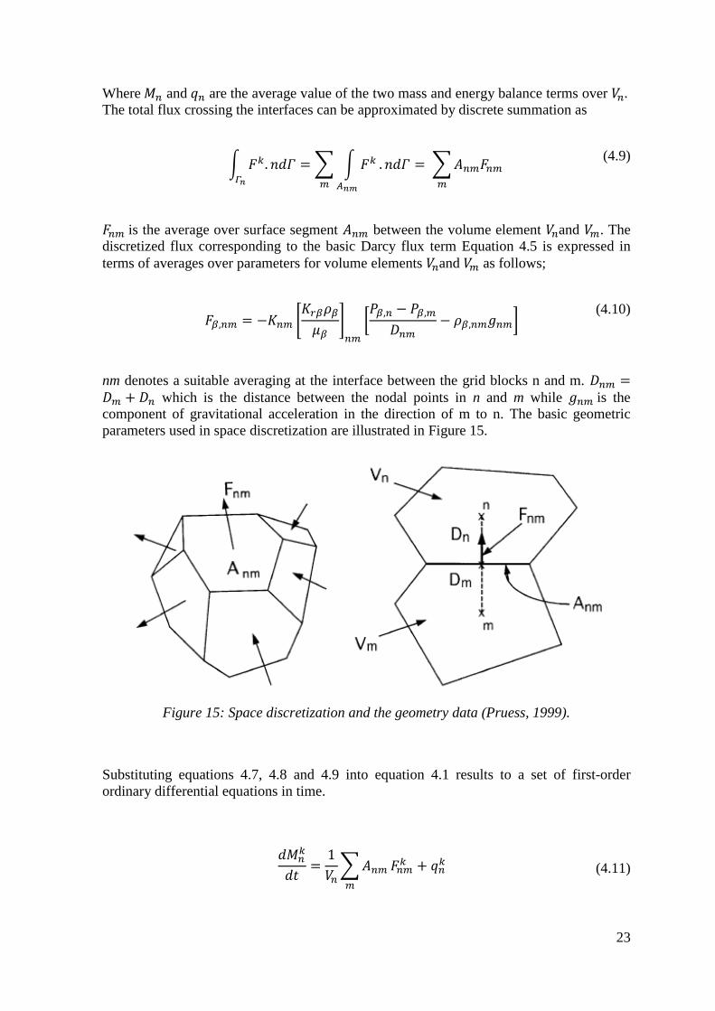
parameters used in space discretization are illustrated in Figure 15.

Figure 15: Space discretization and the geometry data (Pruess, 1999).

Substituting equations 4.7, 4.8 and 4.9 into equation 4.1 results to a set of first-order

ordinary differential equations in time.

(4.11)

24

Time is discretized as a first order finite difference. The flux, sink and source terms on the

right hand side of the equation 4.11 are evaluated at the new level , to

obtain the numerical stability needed for efficient calculation of multiphase flow. The time

discretization results to equation 4.12 below with introduced as residuals.

(4.12)

Equation 4.12 is solved by Newton-Raphson iteration by introducing an iteration index p

and expand the residual at iteration step p + 1 in a Taylor series in terms of those at index

p.

(4.13)

Retaining only terms up to first order results to;

(4.14)

All terms in the Jacobian matrix are evaluated by numerical differentiation to

achieve maximum flexibility in the manner in which various terms in the governing

equations may depend on the primary thermodynamic variable. Iterations are done until all

the residuals are reduced below a preset convergence tolerance typically chosen as .

(4.15)

25

5 Numerical Model

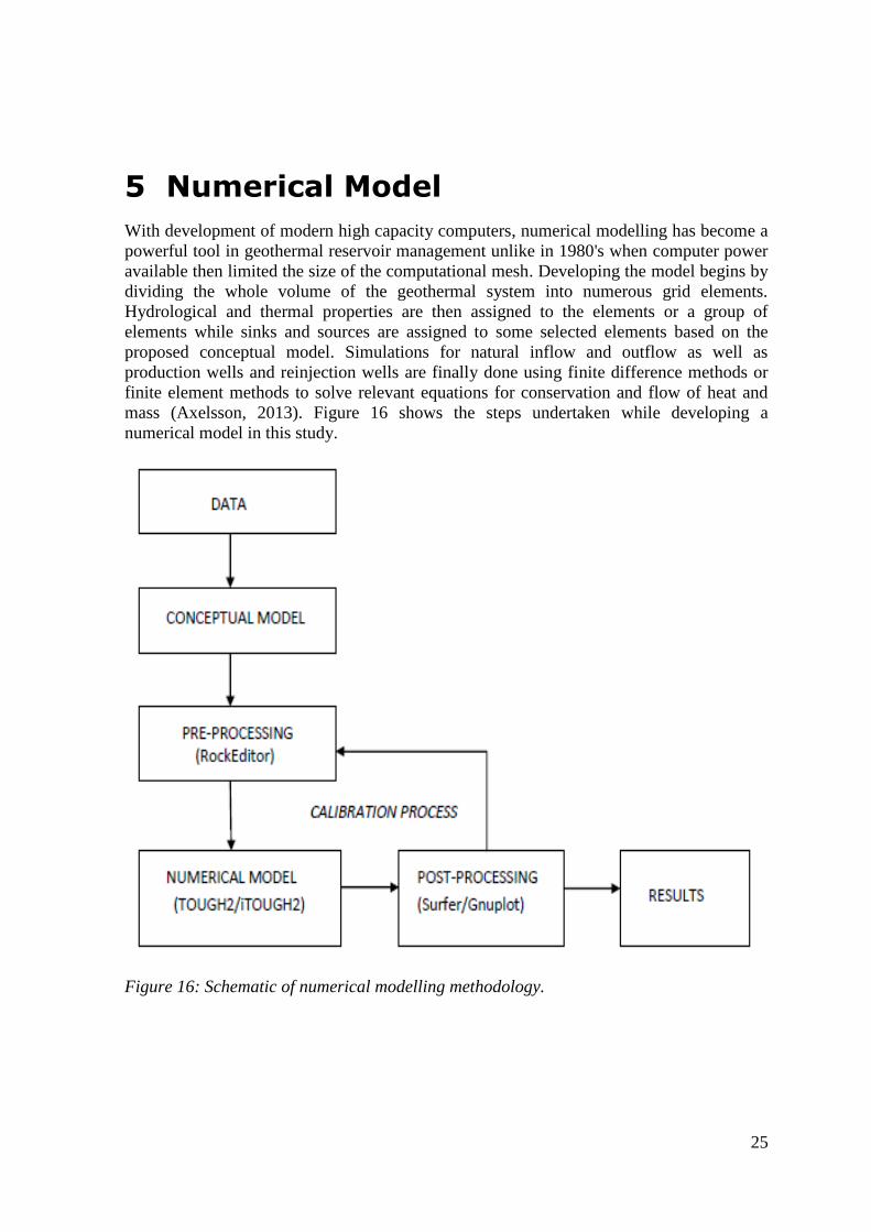
With development of modern high capacity computers, numerical modelling has become a

powerful tool in geothermal reservoir management unlike in 1980's when computer power

available then limited the size of the computational mesh. Developing the model begins by

dividing the whole volume of the geothermal system into numerous grid elements.

Hydrological and thermal properties are then assigned to the elements or a group of

elements while sinks and sources are assigned to some selected elements based on the

proposed conceptual model. Simulations for natural inflow and outflow as well as

production wells and reinjection wells are finally done using finite difference methods or

finite element methods to solve relevant equations for conservation and flow of heat and

mass (Axelsson, 2013). Figure 16 shows the steps undertaken while developing a

numerical model in this study.

Figure 16: Schematic of numerical modelling methodology.

26

5.1 General Mesh Features

5.1.1 Mesh design and boundary conditions

The mesh was set up using RockEditor software package which uses the Amesh program,

a program that generates discrete grids for numerical modelling of flow and transport

problems formulated on integral finite difference method basis. The mesh grid is based on

Voronoi tessellation, a method where a mesh of elements is created within a model domain

with the interface between neighbour elements as the perpendicular bisectors of the line

connecting the element centres. From the element centres, Amesh program computes the

element volume and connection information such as areas, connection distance and the

angle (Haukwa, 1998). The RockEditor software package produces output files suitable for

TOUGH2 simulator input.

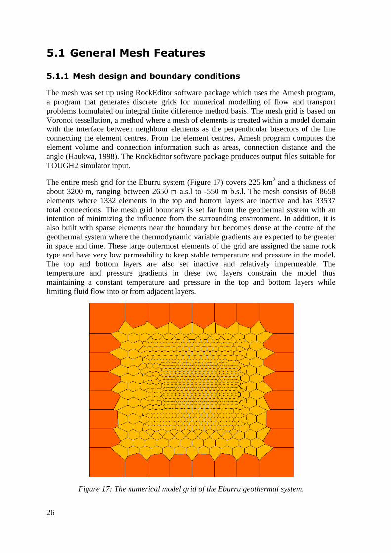
The entire mesh grid for the Eburru system (Figure 17) covers 225 km2 and a thickness of

about 3200 m, ranging between 2650 m a.s.l to -550 m b.s.l. The mesh consists of 8658

elements where 1332 elements in the top and bottom layers are inactive and has 33537

total connections. The mesh grid boundary is set far from the geothermal system with an

intention of minimizing the influence from the surrounding environment. In addition, it is

also built with sparse elements near the boundary but becomes dense at the centre of the

geothermal system where the thermodynamic variable gradients are expected to be greater

in space and time. These large outermost elements of the grid are assigned the same rock

type and have very low permeability to keep stable temperature and pressure in the model.

The top and bottom layers are also set inactive and relatively impermeable. The

temperature and pressure gradients in these two layers constrain the model thus

maintaining a constant temperature and pressure in the top and bottom layers while

limiting fluid flow into or from adjacent layers.

Figure 17: The numerical model grid of the Eburru geothermal system.

27

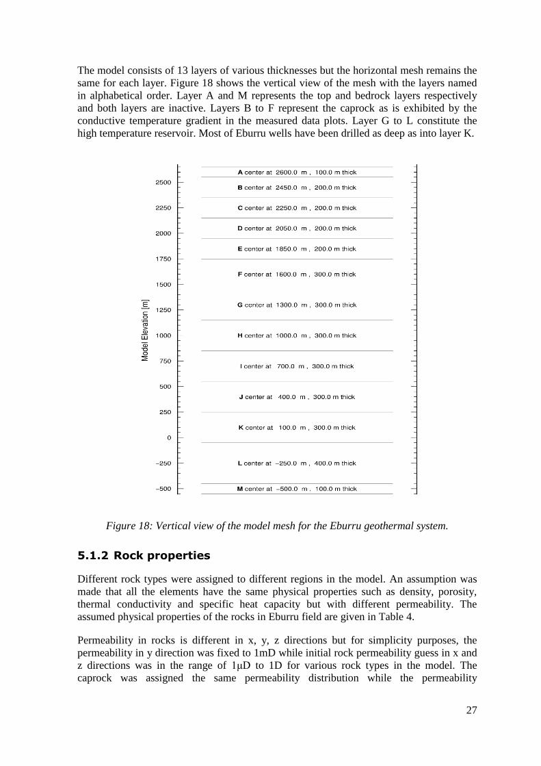
The model consists of 13 layers of various thicknesses but the horizontal mesh remains the

same for each layer. Figure 18 shows the vertical view of the mesh with the layers named

in alphabetical order. Layer A and M represents the top and bedrock layers respectively

and both layers are inactive. Layers B to F represent the caprock as is exhibited by the

conductive temperature gradient in the measured data plots. Layer G to L constitute the

high temperature reservoir. Most of Eburru wells have been drilled as deep as into layer K.

Figure 18: Vertical view of the model mesh for the Eburru geothermal system.

5.1.2 Rock properties

Different rock types were assigned to different regions in the model. An assumption was

made that all the elements have the same physical properties such as density, porosity,

thermal conductivity and specific heat capacity but with different permeability. The

assumed physical properties of the rocks in Eburru field are given in Table 4.

Permeability in rocks is different in x, y, z directions but for simplicity purposes, the

permeability in y direction was fixed to 1mD while initial rock permeability guess in x and

z directions was in the range of 1μD to 1D for various rock types in the model. The

caprock was assigned the same permeability distribution while the permeability

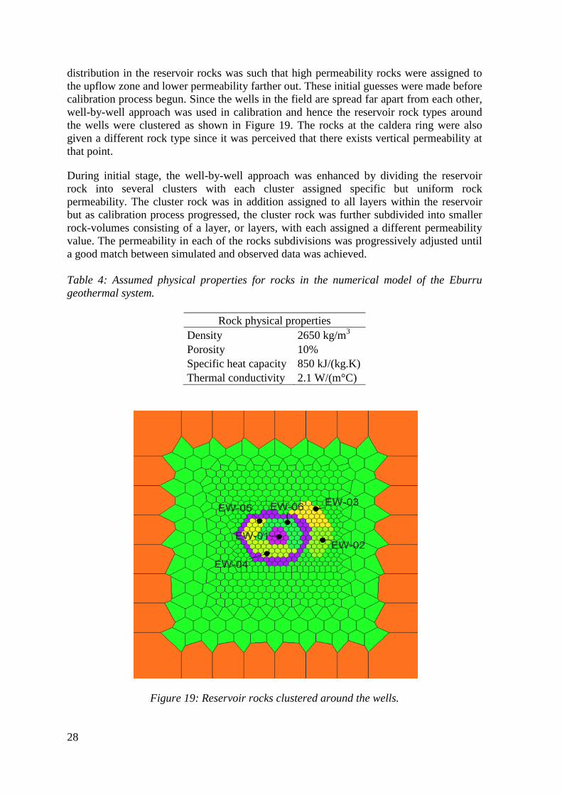
28

distribution in the reservoir rocks was such that high permeability rocks were assigned to

the upflow zone and lower permeability farther out. These initial guesses were made before

calibration process begun. Since the wells in the field are spread far apart from each other,

well-by-well approach was used in calibration and hence the reservoir rock types around

the wells were clustered as shown in Figure 19. The rocks at the caldera ring were also

given a different rock type since it was perceived that there exists vertical permeability at

that point.

During initial stage, the well-by-well approach was enhanced by dividing the reservoir

rock into several clusters with each cluster assigned specific but uniform rock

permeability. The cluster rock was in addition assigned to all layers within the reservoir

but as calibration process progressed, the cluster rock was further subdivided into smaller

rock-volumes consisting of a layer, or layers, with each assigned a different permeability

value. The permeability in each of the rocks subdivisions was progressively adjusted until

a good match between simulated and observed data was achieved.

Table 4: Assumed physical properties for rocks in the numerical model of the Eburru

geothermal system.

Rock physical properties

Density 2650 kg/m3

Porosity 10%

Specific heat capacity 850 kJ/(kg.K)

Thermal conductivity 2.1 W/(m°C)

Figure 19: Reservoir rocks clustered around the wells.

29

5.1.3 Initial conditions

The fluid in the numerical model was assumed to be pure water. All water properties into

the TOUGH2 model simulations were thus obtained from equation-of-state module EOS1

which contains steam table equations as given by the International Formulation Committee

(1967). The flow systems in the model were initialised by assigning a complete set of

primary thermodynamic variables to all grid blocks into which the flow domain was

discretized (Pruess et al., 1999).

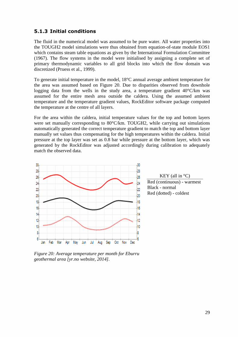
To generate initial temperature in the model, 18°C annual average ambient temperature for

the area was assumed based on Figure 20. Due to disparities observed from downhole

logging data from the wells in the study area, a temperature gradient 40°C/km was

assumed for the entire mesh area outside the caldera. Using the assumed ambient

temperature and the temperature gradient values, RockEditor software package computed

the temperature at the centre of all layers.

For the area within the caldera, initial temperature values for the top and bottom layers

were set manually corresponding to 80°C/km. TOUGH2, while carrying out simulations

automatically generated the correct temperature gradient to match the top and bottom layer

manually set values thus compensating for the high temperatures within the caldera. Initial

pressure at the top layer was set as 0.8 bar while pressure at the bottom layer, which was

generated by the RockEditor was adjusted accordingly during calibration to adequately

match the observed data.

Figure 20: Average temperature per month for Eburru

geothermal area [yr.no website, 2014].

KEY (all in °C)

Red (continuous) - warmest

Black - normal

Red (dotted) - coldest

30

5.2 Natural State Model

Natural state modelling simulates the physical state of a geothermal field prior to

production (Axelsson, 2013). The model is developed to verify the validity of conceptual

models and to quantify the natural flow within the system (Bodvarsson et al., 1989). It

consists running a model for a long time in a simulation of the development of the

geothermal field over a geological time (O' Sullivan et al., 2001). This was achieved in this

study by setting the simulation time to be very long (about 200,000 years) and running the

simulator until steady-state was reached. At steady-state, the heat and mass entering into

the model are equal to heat and mass released through the model boundaries and thus no

change is observed in thermodynamic variables. This was taken as the natural pre-

exploitation state model. According to Grant and Bixley (2011), the natural state of a

reservoir depends only on rock permeability, at a given inflow.

The model was constructed with an input of mass and heat at the bottom. Guided by the

conceptual model proposed in part 2.5, a mass source was set in 6 elements around well

EW-01 in layer L, a layer above the inactive bedrock where the upflow was perceived to

be located in the reservoir. The mass source supplied fluid of constant enthalpy with

constant mass flowrate. Simulation was done and once steady-state was reached, the

temperature and pressure distributions in the model were matched with measured field

data. The permeability distribution, the strength of the mass and heat upflow into the

system were adjusted. The location of the upflow was adjusted somewhat, as well. The

model was then re-run until steady-state was achieved and the process was repeated until a

satisfactory match between the calculated and measured data was achieved. To achieve the

best match between the measured and simulated data, a total of 15kg/s of fluid with an

enthalpy of around 1260kJ/kg was injected into the 6 elements in the model, giving a

thermal input of about 18.9 MWt.

In this study, the natural state was achieved by adjusting the permeability distribution,

strength of the heat and mass flow manually until an acceptable natural state match was

achieved. It took considerable amount of time but the good practice proposed by Grant and

Bixley (2011) was followed, which suggests starting with low permeability then increasing

it gradually until a good match is achieved. Automatic calibration was later attempted with

iTOUGH2, but the results obtained were similar to those obtained through the manual

calibration process. The results of the natural state model are presented in part 5.5 and in

Appendix C.

5.3 Production History Model

The natural state model earlier developed serves as an input, and as initial conditions, for

the production history model which describes the response of a reservoir to exploitation. It

refines the numerical model earlier calibrated by natural state model in readiness for future

production predictions from the study field. Simulation of the total production period

begins by assigning the past production for the well to relevant blocks in the model based

on information about the locations of the feed-zones. The entire data set is then calibrated

in a single run, that is, the system is driven to steady-state after which it proceeds

automatically to the production phase. All the results are finally compared to the measured

31

values and a decision based on that comparison is made by iTOUGH2 to continue to the

next calibration run.

In this study, flowing wells were simulated in the model by forced mass extraction per time

unit using option MASS in TOUGH2 simulator. The mass extracted from the well was

specified in the model calculations and only the enthalpy of the fluid extracted was used in

calibration of the model. Well EW-01 has been in production from 2012 and has been

supplying steam to a 2.5 MWe power plant since then. Eburru geothermal system therefore

has a very short production history but an attempt was made to calibrate the model using

the production data available now. The data available from the field included separation

pressure, steam flow and brine flow all captured by data loggers.

Fluid enthalpy at wellhead which was used in calibrating Eburru model was obtained

theoretically through an approach presented by Grant and Bixley (2011). Using the

approach, the total mass flow was obtained by summing the steam and brine flows since

both flows were measured at the same separation pressure.

(5.1)

Where and represents steam and brine flow rate respectively. The dryness fraction X

was obtained by the equation;

(5.2)

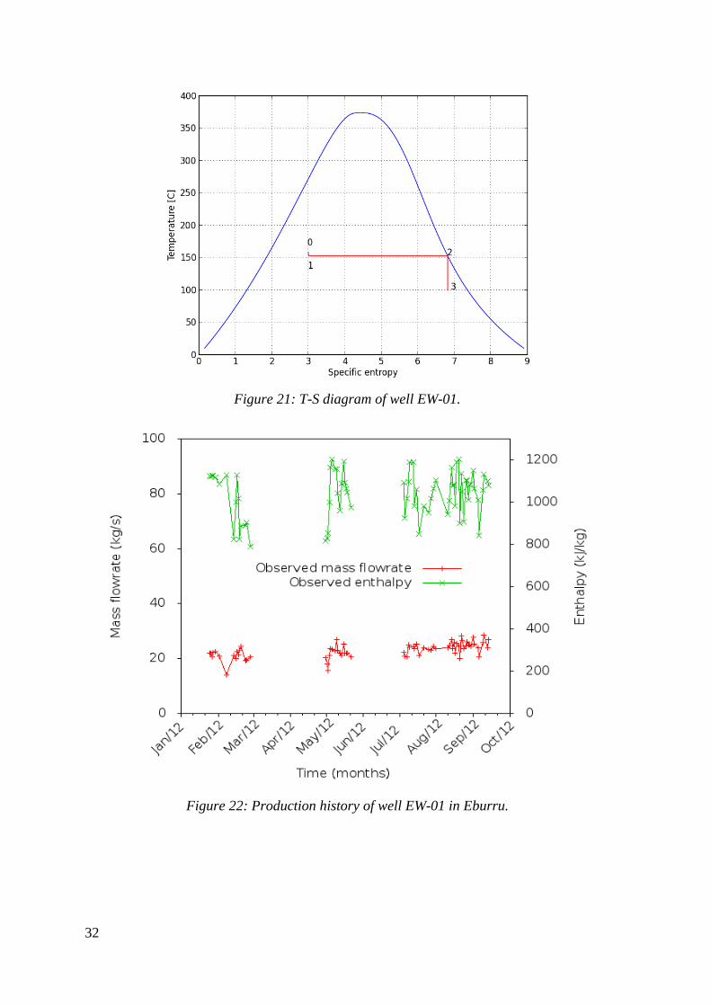
The fluid extracted from the well undergoes an isenthalpic process from the wellhead

(point 0 in Figure 21) to the steam separator (point 1 in Figure 21). The enthalpy of the

fluid at the wellhead was calculated as

(5.3)

Where and represents saturated liquid and steam enthalpies at the separation

pressure respectively. The enthalpy was calculated using Xsteam (IAPWS IF97

formulation by Holmgren) by calling h_px(h20) where separation pressure from the data

loggers and X calculated in equation 5.2 were used. The enthalpy at the turbine inlet (point

2 in Figure 21) is saturated steam enthalpy at the separator pressure while point 3 (Figure

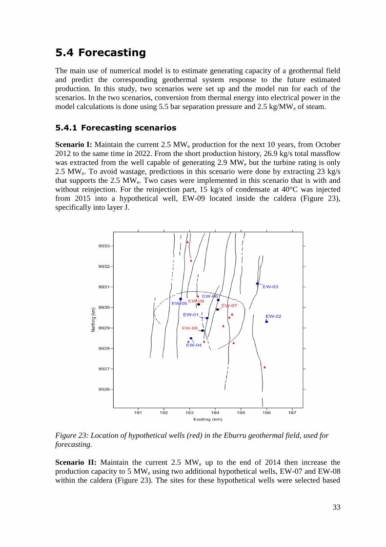
21) is the turbine exhaust fluid enthalpy at the condenser pressure. Figure 22 shows the

mass flow from well EW-01 and the corresponding enthalpy for a period of 8 months. The

reason for shutting the well was not known but an assumption was made that the power

plant had some technical problems.

The temperature plot for well EW-01 (Figure A.1 in Appendix A) shows that the well has

the major feed zone at the well bottom. To carry out production matching simulations, the

computed values for mass flow and enthalpy were assigned to the element in Layer K that

contains the well feed-zone. The results of the production history model are presented in

part 5.5.

32

Figure 21: T-S diagram of well EW-01.

Figure 22: Production history of well EW-01 in Eburru.

33

5.4 Forecasting

The main use of numerical model is to estimate generating capacity of a geothermal field

and predict the corresponding geothermal system response to the future estimated

production. In this study, two scenarios were set up and the model run for each of the

scenarios. In the two scenarios, conversion from thermal energy into electrical power in the

model calculations is done using 5.5 bar separation pressure and 2.5 kg/MWe of steam.

5.4.1 Forecasting scenarios

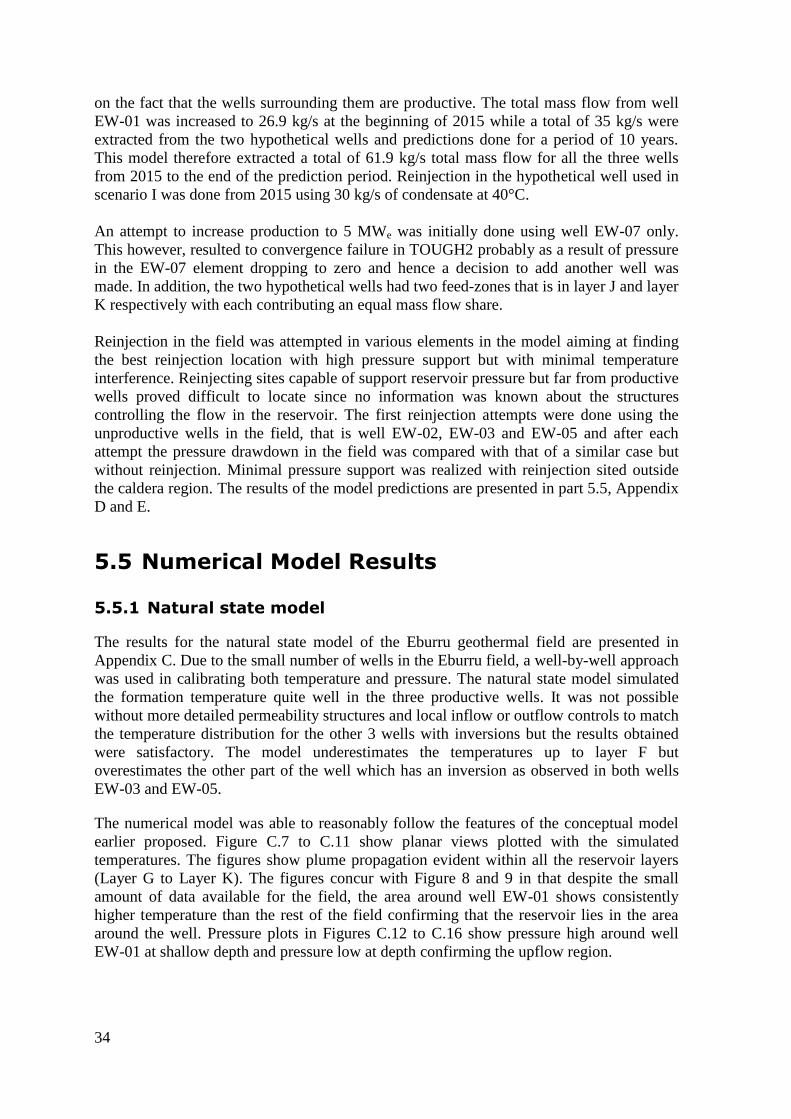
Scenario I: Maintain the current 2.5 MWe production for the next 10 years, from October

2012 to the same time in 2022. From the short production history, 26.9 kg/s total massflow

was extracted from the well capable of generating 2.9 MWe but the turbine rating is only

2.5 MWe. To avoid wastage, predictions in this scenario were done by extracting 23 kg/s

that supports the 2.5 MWe. Two cases were implemented in this scenario that is with and

without reinjection. For the reinjection part, 15 kg/s of condensate at 40°C was injected

from 2015 into a hypothetical well, EW-09 located inside the caldera (Figure 23),

specifically into layer J.

Figure 23: Location of hypothetical wells (red) in the Eburru geothermal field, used for

forecasting.

Scenario II: Maintain the current 2.5 MWe up to the end of 2014 then increase the

production capacity to 5 MWe using two additional hypothetical wells, EW-07 and EW-08

within the caldera (Figure 23). The sites for these hypothetical wells were selected based

34

on the fact that the wells surrounding them are productive. The total mass flow from well

EW-01 was increased to 26.9 kg/s at the beginning of 2015 while a total of 35 kg/s were

extracted from the two hypothetical wells and predictions done for a period of 10 years.

This model therefore extracted a total of 61.9 kg/s total mass flow for all the three wells

from 2015 to the end of the prediction period. Reinjection in the hypothetical well used in

scenario I was done from 2015 using 30 kg/s of condensate at 40°C.

An attempt to increase production to 5 MWe was initially done using well EW-07 only.

This however, resulted to convergence failure in TOUGH2 probably as a result of pressure

in the EW-07 element dropping to zero and hence a decision to add another well was

made. In addition, the two hypothetical wells had two feed-zones that is in layer J and layer

K respectively with each contributing an equal mass flow share.

Reinjection in the field was attempted in various elements in the model aiming at finding

the best reinjection location with high pressure support but with minimal temperature

interference. Reinjecting sites capable of support reservoir pressure but far from productive

wells proved difficult to locate since no information was known about the structures

controlling the flow in the reservoir. The first reinjection attempts were done using the

unproductive wells in the field, that is well EW-02, EW-03 and EW-05 and after each

attempt the pressure drawdown in the field was compared with that of a similar case but

without reinjection. Minimal pressure support was realized with reinjection sited outside

the caldera region. The results of the model predictions are presented in part 5.5, Appendix

D and E.

5.5 Numerical Model Results

5.5.1 Natural state model

The results for the natural state model of the Eburru geothermal field are presented in

Appendix C. Due to the small number of wells in the Eburru field, a well-by-well approach

was used in calibrating both temperature and pressure. The natural state model simulated

the formation temperature quite well in the three productive wells. It was not possible

without more detailed permeability structures and local inflow or outflow controls to match

the temperature distribution for the other 3 wells with inversions but the results obtained

were satisfactory. The model underestimates the temperatures up to layer F but

overestimates the other part of the well which has an inversion as observed in both wells

EW-03 and EW-05.

The numerical model was able to reasonably follow the features of the conceptual model

earlier proposed. Figure C.7 to C.11 show planar views plotted with the simulated

temperatures. The figures show plume propagation evident within all the reservoir layers

(Layer G to Layer K). The figures concur with Figure 8 and 9 in that despite the small

amount of data available for the field, the area around well EW-01 shows consistently

higher temperature than the rest of the field confirming that the reservoir lies in the area

around the well. Pressure plots in Figures C.12 to C.16 show pressure high around well

EW-01 at shallow depth and pressure low at depth confirming the upflow region.

35

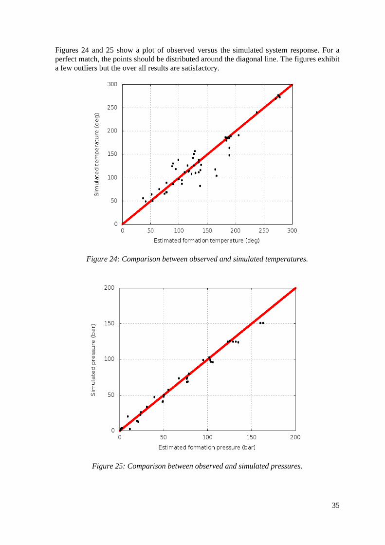
Figures 24 and 25 show a plot of observed versus the simulated system response. For a

perfect match, the points should be distributed around the diagonal line. The figures exhibit

a few outliers but the over all results are satisfactory.

Figure 24: Comparison between observed and simulated temperatures.

Figure 25: Comparison between observed and simulated pressures.

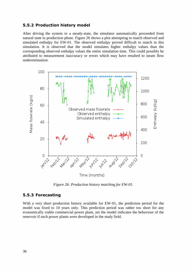
36

5.5.2 Production history model

After driving the system to a steady-state, the simulator automatically proceeded from

natural state to production phase. Figure 26 shows a plot attempting to match observed and

simulated enthalpy for EW-01. The observed enthalpy proved difficult to match in this

simulation. It is observed that the model simulates higher enthalpy values than the

corresponding observed enthalpy values the entire simulation time. This could possibly be

attributed to measurement inaccuracy or errors which may have resulted to steam flow

underestimation.

Figure 26: Production history matching for EW-01.

5.5.3 Forecasting

With a very short production history available for EW-01, the prediction period for the

model was fixed to 10 years only. This prediction period was rather too short for any

economically viable commercial power plant, yet the model indicates the behaviour of the

reservoir if such power plants were developed in the study field.

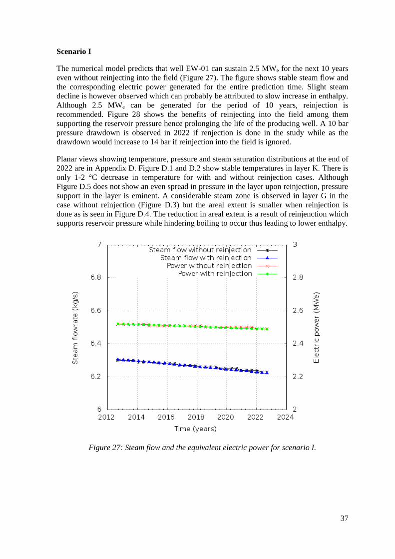
37

Scenario I

The numerical model predicts that well EW-01 can sustain 2.5 MWe for the next 10 years

even without reinjecting into the field (Figure 27). The figure shows stable steam flow and

the corresponding electric power generated for the entire prediction time. Slight steam

decline is however observed which can probably be attributed to slow increase in enthalpy.

Although 2.5 MWe can be generated for the period of 10 years, reinjection is

recommended. Figure 28 shows the benefits of reinjecting into the field among them

supporting the reservoir pressure hence prolonging the life of the producing well. A 10 bar

pressure drawdown is observed in 2022 if renjection is done in the study while as the

drawdown would increase to 14 bar if reinjection into the field is ignored.

Planar views showing temperature, pressure and steam saturation distributions at the end of

2022 are in Appendix D. Figure D.1 and D.2 show stable temperatures in layer K. There is

only 1-2 °C decrease in temperature for with and without reinjection cases. Although

Figure D.5 does not show an even spread in pressure in the layer upon reinjection, pressure

support in the layer is eminent. A considerable steam zone is observed in layer G in the

case without reinjection (Figure D.3) but the areal extent is smaller when reinjection is

done as is seen in Figure D.4. The reduction in areal extent is a result of reinjenction which

supports reservoir pressure while hindering boiling to occur thus leading to lower enthalpy.

Figure 27: Steam flow and the equivalent electric power for scenario I.

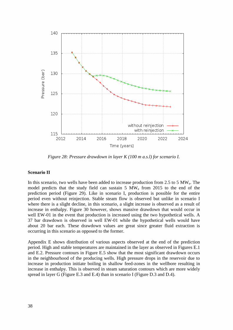
38

Figure 28: Pressure drawdown in layer K (100 m a.s.l) for scenario I.

Scenario II

In this scenario, two wells have been added to increase production from 2.5 to 5 MWe. The

model predicts that the study field can sustain 5 MWe from 2015 to the end of the

prediction period (Figure 29). Like in scenario I, production is possible for the entire

period even without reinjection. Stable steam flow is observed but unlike in scenario I

where there is a slight decline, in this scenario, a slight increase is observed as a result of

increase in enthalpy. Figure 30 however, shows massive drawdown that would occur in

well EW-01 in the event that production is increased using the two hypothetical wells. A

37 bar drawdown is observed in well EW-01 while the hypothetical wells would have

about 20 bar each. These drawdown values are great since greater fluid extraction is

occurring in this scenario as opposed to the former.

Appendix E shows distribution of various aspects observed at the end of the prediction

period. High and stable temperatures are maintained in the layer as observed in Figures E.1

and E.2. Pressure contours in Figure E.5 show that the most significant drawdown occurs

in the neighbourhood of the producing wells. High pressure drops in the reservoir due to

increase in production initiate boiling in shallow feed-zones in the wellbore resulting in

increase in enthalpy. This is observed in steam saturation contours which are more widely

spread in layer G (Figure E.3 and E.4) than in scenario I (Figure D.3 and D.4).

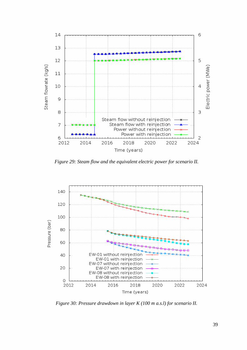
39

Figure 29: Steam flow and the equivalent electric power for scenario II.

Figure 30: Pressure drawdown in layer K (100 m a.s.l) for scenario II.

40

5.6 Sensitivity Analysis

The sensitivity analysis evaluated at the minimum of the objective function contains much

information regarding the impact of the parameters on the system behaviour and how

valuable certain data were in parameter estimation. The results provide an insight into data

sensitivity, parameter influence and correlation between the parameters. According to

Wellmann et al. (2014), the more sensitive a parameter is, and the less correlated it is with

the other parameters, the better it is to estimate its value from the available observations.

The information about sensitivity in the model simulations is provided in the iTOUGH2

output files.

The most influential parameters in the model is the permeability of the reservoir rocks

around well EW-06 followed by the enthalpy of the fluid input and the permeability of

reservoir rocks around well EW-01. It is worth noting that the permeability in the reservoir

rock in well EW-06 has the highest sensitivity to objective function yet there is no

production in that well contrary to the expectation which is that the permeability of the

reservoir rock in well EW-01 should be most sensitive since the well is located at the

inferred upflow zone and hence the mass and heat input into the model is right beneath the

well. From the correlation plot, the horizontal permeability in wells EW-02 and EW-03

show the highest positive correlation between its rock clusters indicating possibility of over

parameterization in the clusters.

From the analysis, it is evident that the model is not fully constrained and thus can be

regarded as partly calibrated. This can be attributed to the small number of wells in the

study field and the short production history from well EW-01, the only well under

utilization.

41

6 Conclusions

In this study, a conceptual model of the Eburru geothermal system has been developed on

basis of the goescientific information available. The conceptual model reveals only one

upflow zone in the field with an inferred heat source below well EW-01. This coincides

well with the geophysical analysis at depth that shows a low resistive zone attributed to the

heat source. It is evident from the model that the hot fluid flows upwards in the centre of

the system and then outflows at around 1500 m a.s.l. The conceptual model suggests that

the geothermal resource is within the caldera only and with recharge from all directions.

Intensive research on how to demarcate reservoir extent was performed and two

approaches arrived at. The results from the preferred approach showed that Eburru

geothermal resource covers an area ranging from 1-6 km2 and is within the caldera only as

described by the conceptual model. The resource area and thickness, together with other

parameters was used to estimate the electric power production capacity using Monte Carlo

simulations, a volumetric method analysis tool that caters for uncertainty. The results from

the Monte Carlo method indicate that the resource should sustain at least 7-11 MWe for a

period of 30-50 years. The simulations are reasonable and realistic but cannot be fully

relied on since the volumetric model does not consider the recharge from boundaries,

pressure decline and phase transition of the reservoir to exploitation and hence cannot

validate the sustainability of the generating capacity it yields.

The first numerical model of Eburru geothermal resource has been developed. The

numerical model was built using natural state and a very short production history data

available and could be described as partly calibrated. This is because only 6 wells were

used to explain the global understanding of Eburru geothermal field in addition to 8

months production history and this does not provide adequate constraints on the model.

The model mesh covers an area of 225 km2 and has 13 layers with a well-by-well approach

used in calibrating the wells. The temperature distribution for the productive wells was

adequately matched while the rest of the wells with an inversion proved difficult to match

exactly, but the results were quite satisfactory. Acceptable pressure distribution was also

obtained for almost all wells. The results of forward modelling estimated that about 15 kg/s

of 1260 kJ/kg fluid is injected into the model below well EW-01 where the upflow is

perceived to be in the Eburru geothermal system. Planar views generated from the

simulated data are in agreement with the conceptual model.

The calibrated numerical model was used in forecasting scenarios to predict the reservoir's

response to future exploitation. Two scenarios were considered where reinjection and no

reinjection cases were set out for each scenario. The results show that the geothermal

resource can sustain double the current electric power production with reinjection in the

field or without. To double electric power production, two hypothetical wells were used

since convergence failure occurred in TOUGH2 when one well was used. Convergence

failure was a clear sign that another well was required. Production from the two wells was

distributed in two feed-zones per well. Stable supply of steam with stable enthalpy has

42

been realised from the two prediction scenarios. There is no sign of cooling in the reservoir

at the end of the prediction period.

From this study, capabilities and limitations have been observed in simulating a reservoir

with a few wells and a short production history. Although predictions are calculated for a

limited period, the model can bring out the important aspects of the reservoir performance

that may affect development plans. The Eburru model can be validated in future by

comparing the observed actual behaviour from the producing well with the model

prediction, and consequently updated.

In the future, the numerical model needs refining, recalibrating and upgrading with

increase in database. Emphasis should be put on collecting more and accurate production

data from the producing well. In addition, a reinjection study involving tracer tests should

be carried out to realise the best reinjection sites.

43

References

Axelsson, G., Björnsson, G., and Stefánsson, V., 2004: Sustainable utilization of

geothermal resources for 100-300 years. Proceedings of the Twenty-Ninth workshop on

Geothermal Reservoir Engineering, Stanford, California, 9pp.

Axelsson, G., 2008: Management of geothermal resources. Proceedings of the workshop

for decision makers on district heating use of geothermal resources in Asia, organised by

UNU-GTP, TBLRREM and TBGMED, Tianjin, China, 15pp.

Axelsson, G., 2008: Production capacity of geothermal systems. Proceedings of the

workshop for decision makers on district heating use of geothermal resources in Asia,

organised by UNU-GTP, TBLRREM and TBGMED, Tianjin, China, 14pp.

Axelsson, G., Arnaldsson, A., Ármannsson, H., Árnason, K., Einarsson, G., Franzson, H.,

Fridriksson, T., Gudmundsson, G., Gylfadottir, S.S., Halldórsdóttir, S., Hersir, G.P.,

Mortensen, A.K., Thordarson, S., Jóhannesson, S., Bore, C., Karingithi, C., Koech, V.,

Mbithi, U., Muchemi, G., Mwarania, F., Kizito, O., and Ouma, P., 2013: Updated

conceptual model and capacity estimates for the Greater Olkaria Geothermal System,

Kenya. Proceedings of the 38th workshop on Geothermal Reservoir Engineering, Stanford

University, California, 16pp

Axelsson, G., Arnaldsson, A., Gylfadottir, S.S., Halldórsdóttir, S., Mortensen, A.K., Bore,

C., Karingithi, C., Koech, V., Mbithi, U., Muchemi, G., Mwarania, F., Kizito, O., and

Ouma, P., 2013: Conceptual model and resource assessment for the Olkaria Geothermal

System, Kenya. Proceedings of a short course v on conceptual modelling of geothermal

systems, organised by UNU-GTP and LaGeo, Santa Tecla, Elsavador, 21pp.

Axelsson, G., 2013: Dynamic modelling of geothermal systems. Proceedings of a short

course v on conceptual modelling of geothermal systems, organised by UNU-GTP and

LaGeo, Santa Tecla, Elsavador, 21pp.

Beltran, J. M.V., 2003: The origin of pantellerites and the geology of the Eburru volcanic

complex, kenya rift, Africa.MSc. Thesis, The University of Texas at El Paso.

Bodvarsson, G., and Witherspoon, P., 1989: Geothermal reservoir engineering, part I.

Geothermal Science and Technology, 2(1), 1-68.

Fridleifsson, I.B., Bertani, R., Huenges, E., Lund, W.J., Ragnarsson, A., and Rybach, L.,

2008. The possible role and contribution of geothermal energy to the mitigation of climate

change. Proceedings of O.Hohmeyer and T.Trittin (Eds.) IPCC Scoping Meeting on

renewable energy sources, Luebeck, Germany.

Grant, M.A., and Bixley, P.F., 2011: Geothermal reservoir engineering. 2nd

edition,

Academic Press, NY, 323pp

Government of the Republic of Kenya, 2007: Kenya vision 2030 the popular version 26pp.

44

Lagat, J.L., 2003: Geology and the geothermal systems of the southern segment of the

Kenyan rift. International Geothermal Conference, Reykjavik.

Haukwa, C.B., 1998: A mesh creating program for the integral finite difference method:

User's manual. Report LBNL-45284, Lawrence Berkeley National Laboratory, Berkeley,

California, 53pp

International Formulation Committee, 1967: A Formulation of the Thermodynamic

Properties of Ordinary Water Substances, IFC Secretariat, Düsseldorf, Germany.

Holmgren, M., 1997: "Excel thermodynamics Tables Add-in 2.0.8". Downloaded

from:www.me.ua.edu/excel

Market Watch – The Wall street Journal, 2014: Olkaria III Geothermal Complex in Kenya

Reaches 110 MW With Commercial Operation of Plant 3 - Geothermal Project Completed

Nearly Three Months Ahead of Schedule. Press release 04-02-

2014, http://www.marketwatch.com/story/olkaria-iii-geothermal-complex-in-kenya-

reaches-110-mw-with-commercial-operation-of-plant-3-2014-02-04

Mathu, W., 2011: Forest plantations and woodlots in Kenya. African Forest Forum, V1,

issue 13.

Mwangi, A., 2011: Joint ID inversion of MT and TEM data from Eburru, Kenya, and

processing of gravity from Theistareykir, NE-Iceland. UNU GTP report 27 pg 635- 668

Muffler, P., and Cataldi, R., 1978: Methods for the regional assessment of geothermal

resources. Geothermics v7, 53-89.

Muchemi, G., 1990: Geology of Eburru. Discussion papers for Scientific Review Meeting,

Kenya Power Company Limited, internal report.

Ofwona, C.O., 2002: A reservoir study of Olkaria East geothermal system, Kenya.

University of Iceland, M.Sc. thesis, UNU-GTP, Iceland, report 1, 86 pp.

Ofwona, C., 2007: Geothermal resource assessment - case example, Olkaria I. Proceedings

of a short course II on surface exploration for geothermal resources, organised by UNU-

GTP and KenGen, Naivasha, Kenya, 9pp.

Omenda, P. A., and Karingithi, C.W., 1993: Hydrothermal model of Eburru geothermal

field, Kenya. Geothermal Resources Council, Transactions, 17, 155-160.

Omenda, P,A., Onacha, S,A and Ambusso, W,J,. 1993: Occurence and distribution of high

temperature geothermal systems in Kenya. Proceedings 15th NZ geothermal workshop, pg

241-246.

Omenda, W., ''Interview 2013''.

O' Sullivan M.J., Pruess, K., and Lippmann, M., 2001: State of the art geothermal reservoir

simulation. Geothermics, 30, 395-429.

45

Parini, M., and Riedel, K., 2000: Combining probabilistic volumetric and numerical

simulation approaches to improve estimates of geothermal resource capacity. Proceedings

World Geothermal Congress, Kyushu, Japan, 6pp

Pruess, K., Oldenburg, C., and Moridis, G., 1999: TOUGH2, user's guide version 2.0.

Lawrence Berkeley National Laboratory, 197pp.

Saemundsson, K., 2008: East African Rift System - An overview. Short course III on

Exploration for Geothermal Resources, Kenya, October, 8pp.

Sanyal, S.K., and Sarmiento, Z., 2005: Booking geothermal energy reserves. Transactions,

Geothermal Resources Council, v29, 467-474.

Sarmiento, Z.F., Steingrímsson, B. and Axelsson, G., 2013: Volumetric resource

assessment. Short course on conceptual modelling of the geothermal systems, organised by

UNU-GTP and LaGeo, Santa Tecla, El Salvador, 15pp.

Simiyu, S., 2010: Status of geothermal exploration in Kenya and future plans for its

development. Proceedings of World Geothermal Congress, Bali, Indonesia, 11pp

Stefánsson, V., and Steingrímsson, B.S., 1980: Geothermal logging I, an introduction to

techniques and interpretation. Orkustofnun, Reykjavík, report OS-80017/JHD-09, 117 pp.

Thinkgeoenergy article, 2012: Green Energy Group completed 5 MW wellhead modular plant in

Kenya. Press release on 08-28-2012, http://thinkgeoenergy.com/archives/12145;

http://thinkgeoenergy.com/archives/17668

Velador, J.M., Omenda, P.A and Anthony, E.Y., 2003: An integrated mapping and remote

sensing investigation of the structural control for the fumarole location in the Eburru

volcanic complex , Kenya rift. Geothermal Resources Council, Transactions, 27. October

12-15.

Wameyo, P.M., 2007: Transient electromagnetic and magnetotelluric imaging of Eburru

geothermal field, KenGen internal report, 17pp.

Wellmann, J.F., Finsterle, S., and Croucher, A., 2014: Integrating structural geological data

into the inverse modelling framework of iTOUGH2. Computer & Geosciences 65, Elsevier

Journal, pg 95-109.

Williams, C.F., 2004: Development of revised techniques for assessing geothermal

resources. Proceedings of the Twenty-Ninth workshop on Geothermal Reservoir

Engineering, Stanford, California, 6pp.

Williams, C.F., 2007: Updated methods for estimating recovery factors for geothermal

resources. Proceedings of the Thirty-Second workshop on Geothermal Reservoir

Engineering, Stanford, California, 7pp.

yr.no website, 2014: "Weather statistics for Eburru settlement, Nakuru (Kenya)." Accessed

on 02-27-2014, http://www.yr.no/place/Kenya/Nakuru/Eburru_Settlement/statistics.html

47

A: Temperature and Pressure Plots

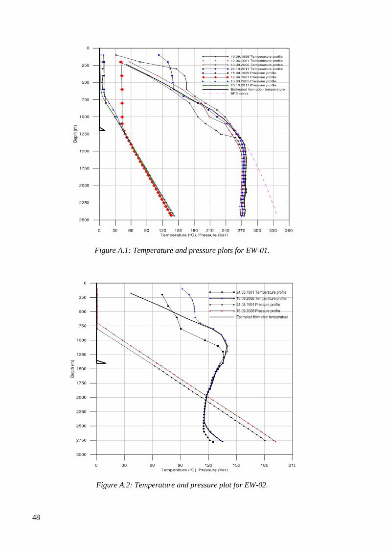
48

Figure A.1: Temperature and pressure plots for EW-01.

Figure A.2: Temperature and pressure plot for EW-02.

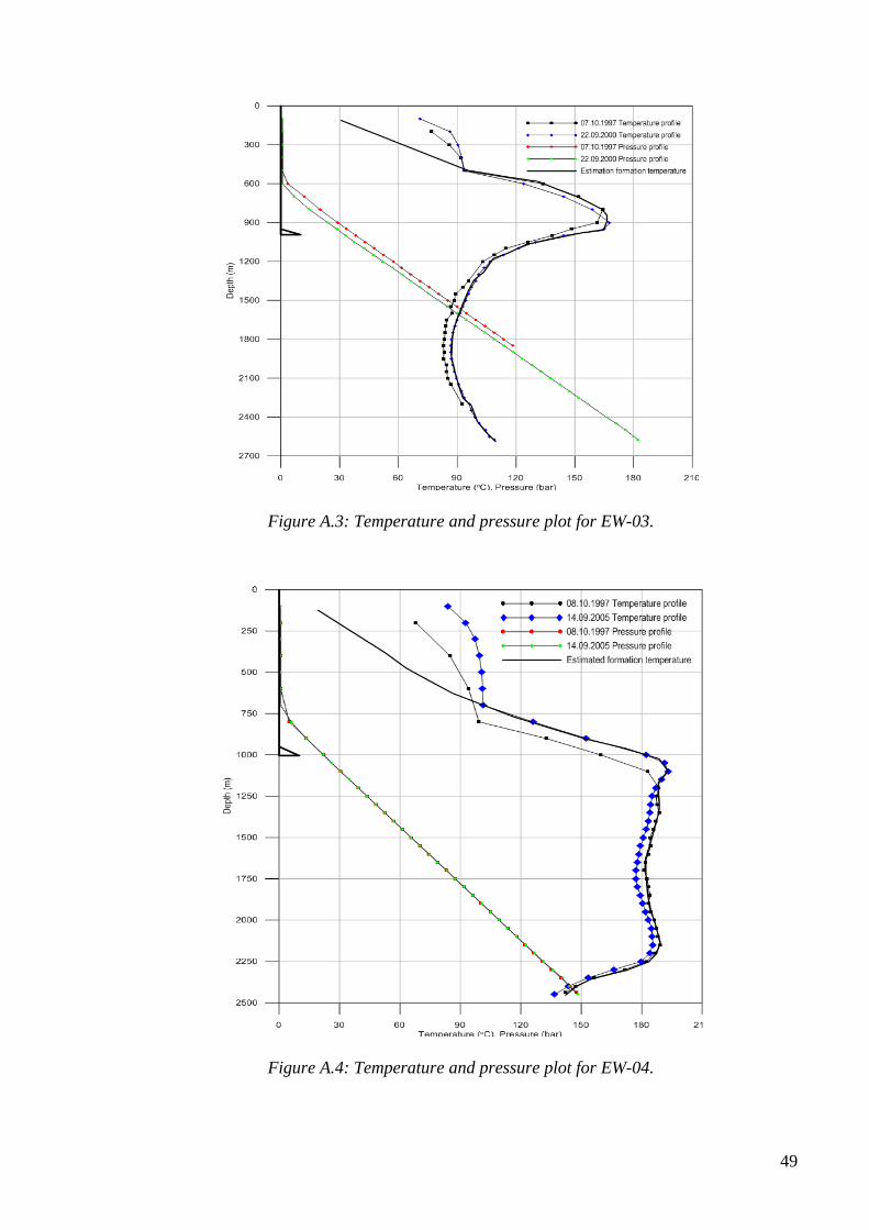
49

Figure A.3: Temperature and pressure plot for EW-03.

Figure A.4: Temperature and pressure plot for EW-04.

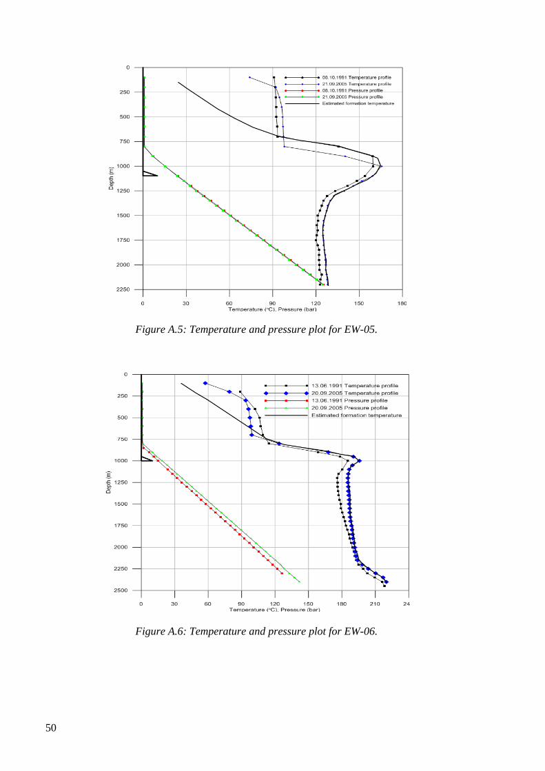
50

Figure A.5: Temperature and pressure plot for EW-05.

Figure A.6: Temperature and pressure plot for EW-06.

51

B: Monte Carlo Simulations

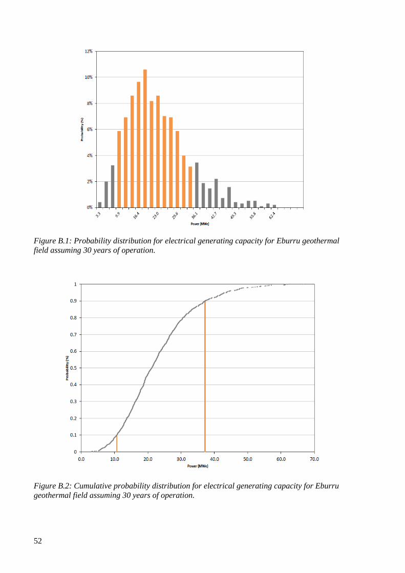
52

Figure B.1: Probability distribution for electrical generating capacity for Eburru geothermal

field assuming 30 years of operation.

Figure B.2: Cumulative probability distribution for electrical generating capacity for Eburru

geothermal field assuming 30 years of operation.

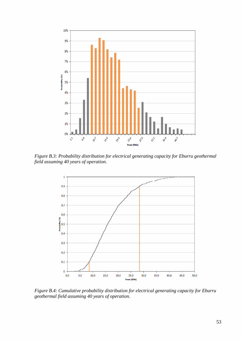
53

Figure B.3: Probability distribution for electrical generating capacity for Eburru geothermal

field assuming 40 years of operation.

Figure B.4: Cumulative probability distribution for electrical generating capacity for Eburru

geothermal field assuming 40 years of operation.

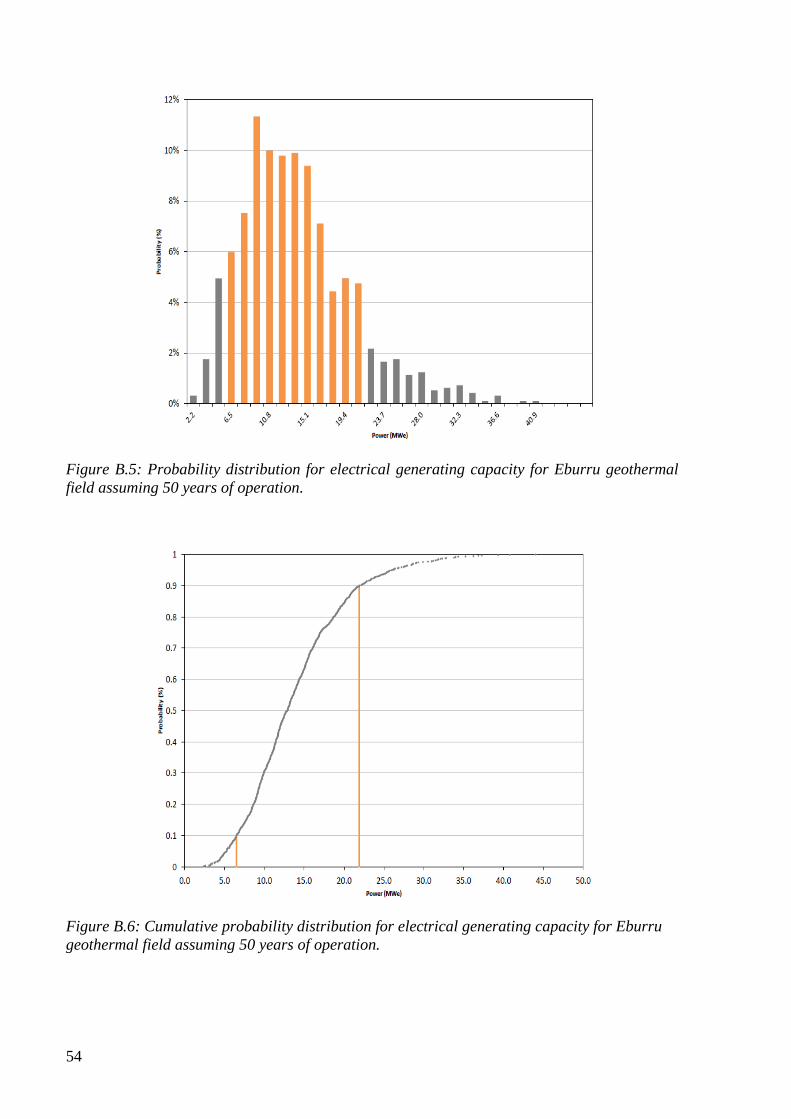
54

Figure B.5: Probability distribution for electrical generating capacity for Eburru geothermal

field assuming 50 years of operation.

Figure B.6: Cumulative probability distribution for electrical generating capacity for Eburru

geothermal field assuming 50 years of operation.

55

C: Natural State Match Results

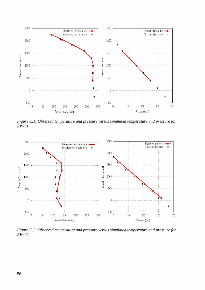
56

Figure C.1: Observed temperature and pressure versus simulated temperature and pressure for

EW-01.

Figure C.2: Observed temperature and pressure versus simulated temperature and pressure for

EW-02.

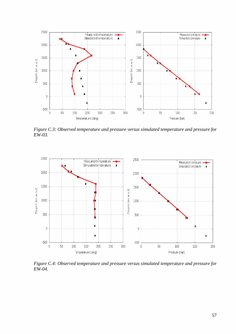
57

Figure C.3: Observed temperature and pressure versus simulated temperature and pressure for

EW-03.

Figure C.4: Observed temperature and pressure versus simulated temperature and pressure for

EW-04.

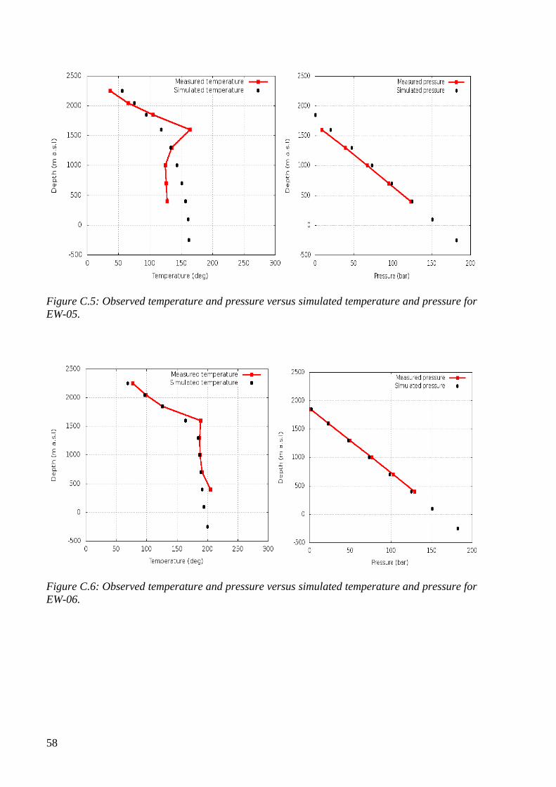
58

Figure C.5: Observed temperature and pressure versus simulated temperature and pressure for

EW-05.

Figure C.6: Observed temperature and pressure versus simulated temperature and pressure for

EW-06.

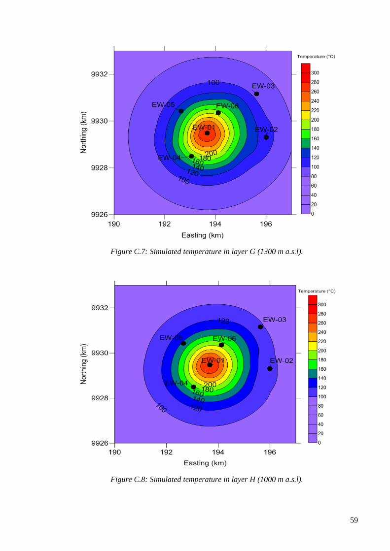
59

Figure C.7: Simulated temperature in layer G (1300 m a.s.l).

Figure C.8: Simulated temperature in layer H (1000 m a.s.l).

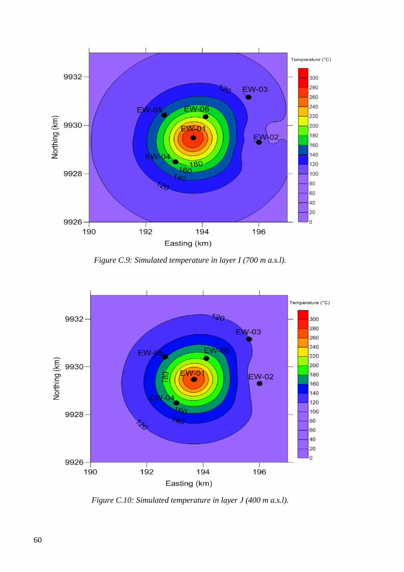
60

Figure C.9: Simulated temperature in layer I (700 m a.s.l).

Figure C.10: Simulated temperature in layer J (400 m a.s.l).

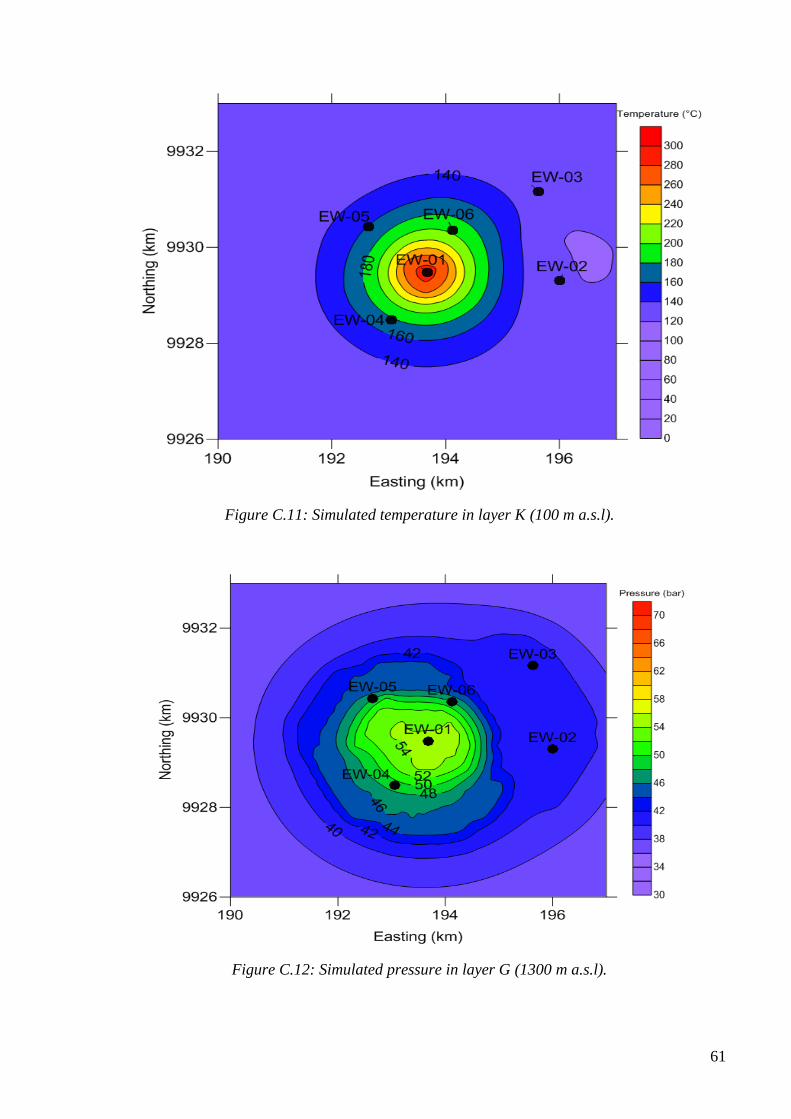
61

Figure C.11: Simulated temperature in layer K (100 m a.s.l).

Figure C.12: Simulated pressure in layer G (1300 m a.s.l).

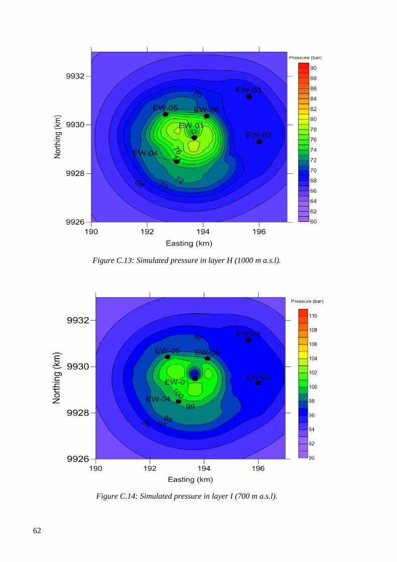
62

Figure C.13: Simulated pressure in layer H (1000 m a.s.l).

Figure C.14: Simulated pressure in layer I (700 m a.s.l).

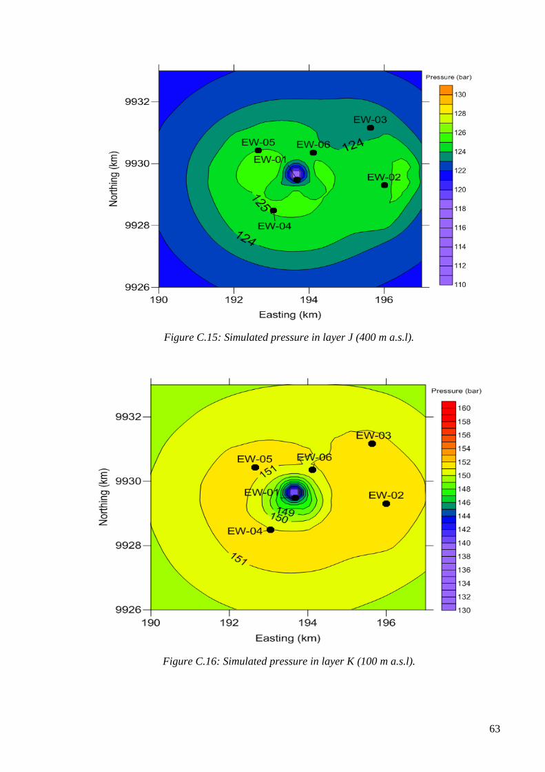
63

Figure C.15: Simulated pressure in layer J (400 m a.s.l).

Figure C.16: Simulated pressure in layer K (100 m a.s.l).

65

D: Results For Scenario I

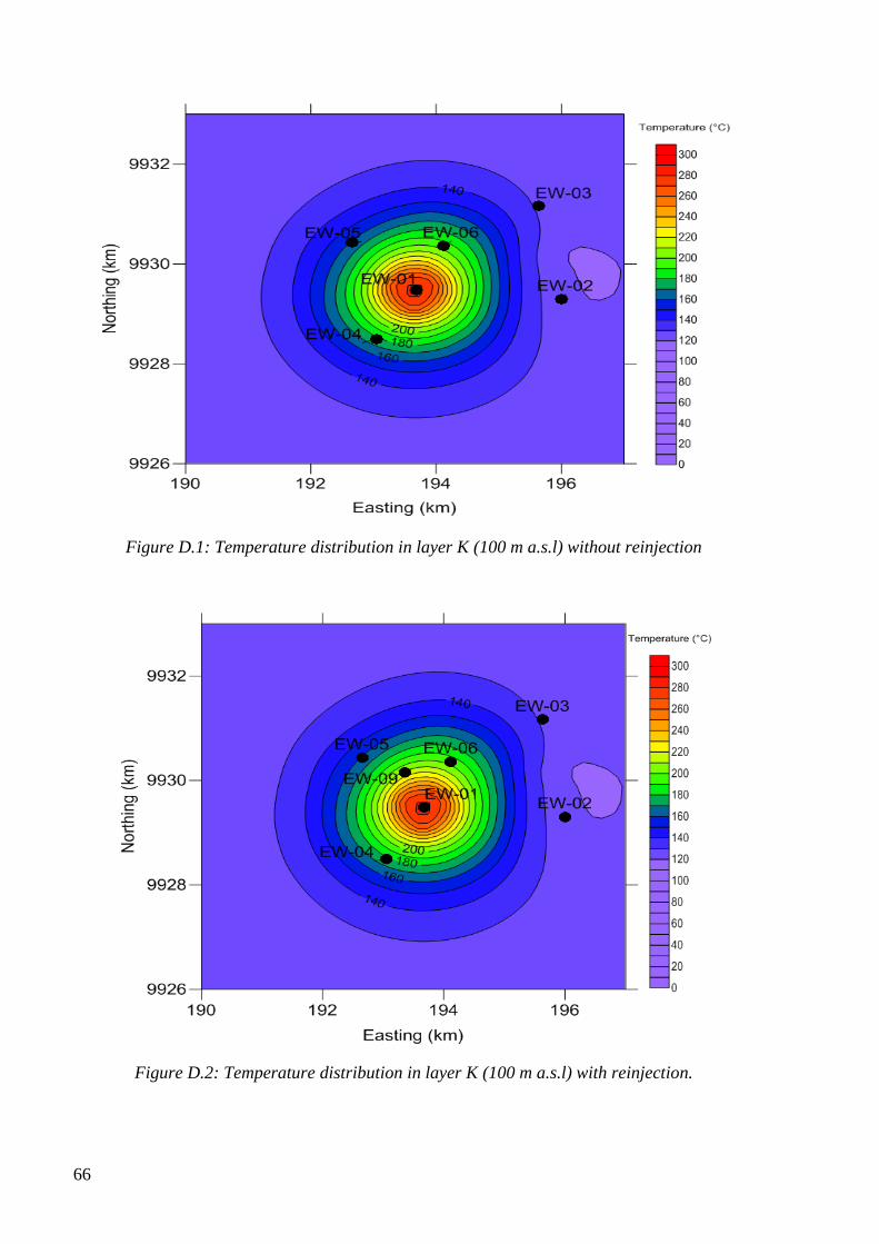
66

Figure D.1: Temperature distribution in layer K (100 m a.s.l) without reinjection

Figure D.2: Temperature distribution in layer K (100 m a.s.l) with reinjection.

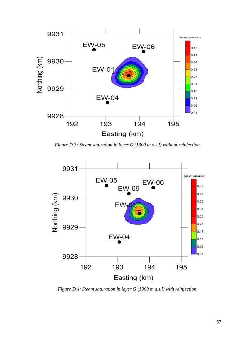
67

Figure D.3: Steam saturation in layer G (1300 m a.s.l) without reinjection.

Figure D.4: Steam saturation in layer G (1300 m a.s.l) with reinjection.

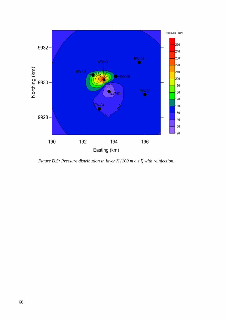
68

Figure D.5: Pressure distribution in layer K (100 m a.s.l) with reinjection.

69

E: Results For Scenario II

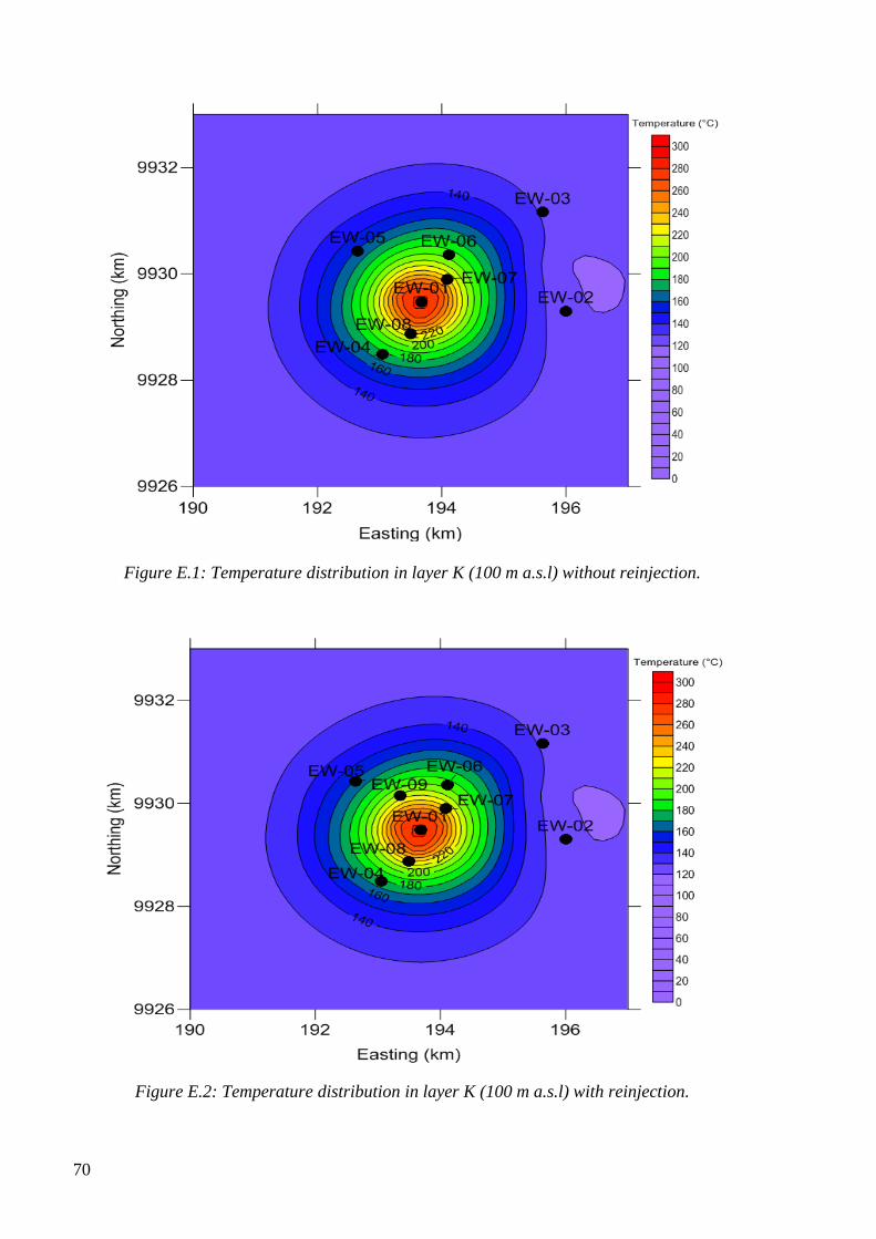
70

Figure E.1: Temperature distribution in layer K (100 m a.s.l) without reinjection.

Figure E.2: Temperature distribution in layer K (100 m a.s.l) with reinjection.

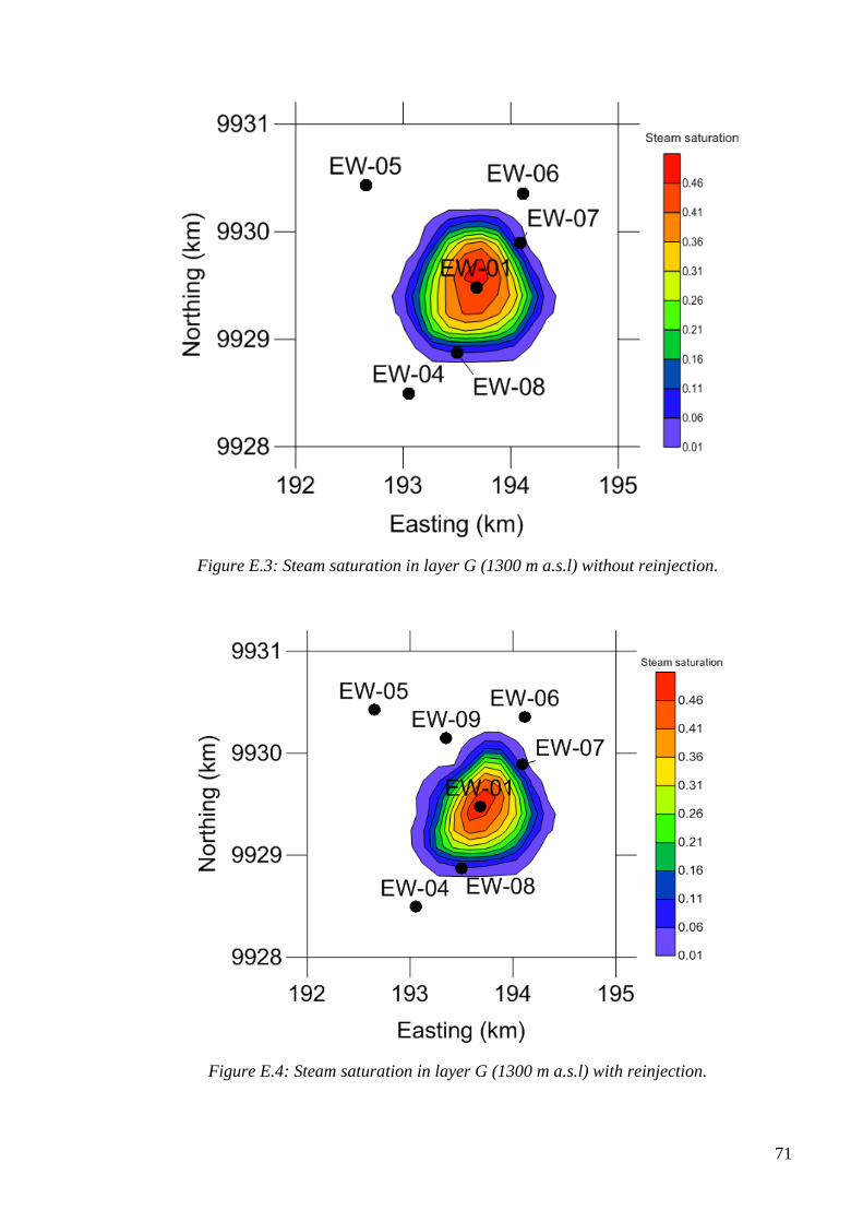
71

Figure E.3: Steam saturation in layer G (1300 m a.s.l) without reinjection.

Figure E.4: Steam saturation in layer G (1300 m a.s.l) with reinjection.

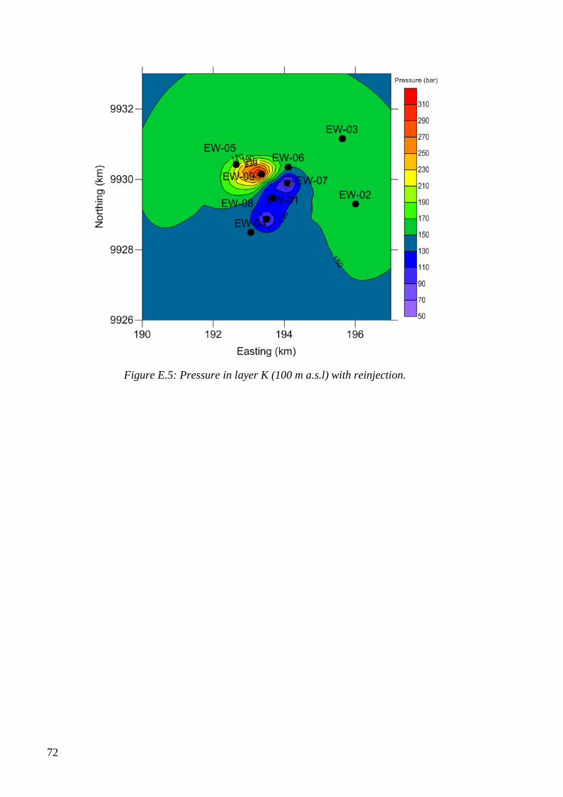
72

Figure E.5: Pressure in layer K (100 m a.s.l) with reinjection.