SPE 6892

by

GEOTHERMALRESERVOIRlIODELLING

K. H. CoatslNTERCGM? Resource Development

and Engineer~ng, Inc.

.

SPE-OfMTOkUII~WAIME

c CopyngrIt 1977. Amerrcan Instdute 01 Mmmg. Metallurgical. and Pef..,bum EnginLefS. Inc

Th!s papef was presented at me 52nd Annual Fall Techmcal Conference and Exhmmon of the SOC!ety01 PelrOleuM Engineers 01 AIME. IM:S III Denver. Colorado. Ott 9.12, 1977 The material ISsubject10coffecbon by the author Permission to COPYIS reslncted 10 an abslracl of not more Ihan 300 words Wrfte 6200 N Central EXIW. Dallas. %las 75206

ABSTRACT INTRODUCTION

This paper describes and partially This paper describes a numerical modelevaluates an implicit, three-diniensional for simulating geothermal well or reservoirgeothermal reservoir simulation model. The performance. The model is considerably moreevaluation emphasizes stability or time-step general than any described in the literaturetolerance of the implicit finite-difference to date. It treats transient, three-formulation. ln eeveral illustrative multi- dimensional, single- or two-phase fluid flowphase flow problems, the model stably ac- in normal heterogeneous or fractured-matrixcommodated time steps corresponding to grid formations. Both conductive and convectiveblock saturation changes of 80-100% and grid heat flow are accounted for and fluid states

block throughput ratios the order of 108. in the reservoir can range from undersaturated

This compares to our experience of limits of liquid to two-phase steam-water mixtures toSuperheated steam.3 to 10% saturation change and roughly 20,000 h

Aquifer water influx and

throughput ratio with sem”-implicit oil and ecc source/sink terms necessary in simulat-

geothermal reservoir models. ing free convection cells are included in themodel formulation.

The illustrative applications shed somelight on practical aspects of geothermal The primary purpose of the work described

reservoir behavior. Applications include here was evaluation of the capability of an

single- and two-phase single-well behavior, implicit model formulation. Our experiencefractured-matrix reservoir performance and with semi-implicit simulation of petroleum

well test interpretation, and extraction of and geothermal reservoirs has shown time step

energy from fractured hot dry rock. Model restrictions zelated to conditional stability.

stability allow+ inclusion of formation In multiphase flow problems, the maximum

fractures and wellbores as grid blocks. tolerable time step size generally correspondsto a maximwn of 3 to 10 percent saturation

An analytical derivation is presented change in any grid block intone time step.

for a well deliverability reduction factor In some steamflood and geothermal simulations,

which can be used in simulations using large we have found this to result in very small

grid blocks. time steps and correspondingly high computingThe factor accounts for reduced costs,deliverability due to hot water flashing and This work was performed with the

steam expansion accompanying pressure decline hope that the implicit model formulation

near the well. would give unconditional stability with notime step restriction other than that imposedby time truncation error.

Calculated results are presented for avariety of geothermal well and reservoirillustrative problems. Emphasis in connec-tion with these results is placed on thestability or time step tolerance of themodel . However, the applications are also

References and illustrations at end of paper.intended to shed some light on practicalaspects of geothermal reservoir behavior. I

~

2 GEOTHERMAL RESERVOIR MODELLING sP17K$la9

—.

Following description of the implicitmodel formulation, the paper presents ap-plications including singls-well deliver-ability under two-phase flow conditions,depletion of a fractured-matrix formationwith boiling, drawdown test interpretation insingle-phase, fractured-matrix formations,and heat extraction from artificitilly frac-tured hot dry rock. An analytical expressionis deri~~d to represent the effective tran-sient pr ductivity index of a well whichexperiences hot water flashing due to pres-sure drawdown from an exterior radius wheresteam saturation may be zero or small.

We have applied the model extensively insimulation of natural convection cells withzero porosity (hard rock) grid block defini-tion above and below the formation. Thisdefinition eliminates the’erroneous imposi-tion of constant temperature boundaries atthe top and bottom of the convection cellcommon in many reported studies ofkaturalconvection. Another application simulateddevelopment over geologic time of a super-heated (Geyser’s type) reservoir from anearly time of magma or heat source intrusionbeneath an initial normal gradient cold wateraquifer. These natural convection typeapplications are omitted here due to thesignificant length of the paper. Some ofthis convection work is reported in a recentpaper 11].

MODEL DESCRIPTION

The model consists of two equationsexpressing conservation of mass of H20 and

conservation of energy. These equationsaccount for three-dimensional, single- ortwo-phase fluid flow, convective and con-ductive heat flow in the reservoir andconductive heat transfer between the res-?rvoir and overlying and underlying strata.l’hephase configuration at any time can varyspatially through the formation from single-phase undersaturated water to two-phasesteam-water mixture to single-phasesuperheated steam..

The equations represent water influxfrom an aquifer extending beyond the res-ervoir grid using the Carter-Tracy [2] orsimpler approximations. Heat source and sinkterms in the equations are useful in imposingtemperature and/or heat flux boundary condi-tions in simulation of natural convection.~he model equations do not account for thepresence of inert gases or for varyingconcentration and precipitation of dissolvedsalts.

The model applies to reservoir gridsincluding one-dimensional, two-dimen-sional radial-z, x-z or x-y and three-dimensional, either x-y-z Cartesian orr-0-z cylindrical. In the r-z and r-0-zcase, the wellbore of a well at r = O can beincluded in the grid, resulting in enhancedstability and accuracy as discussed below.The r-z grid can be used in simulating asector of a fractured-matrix reservoir withthe horizontal and vertical fractures rep-resented by grid blocks. The grid caninclude blocks of zero porosity representinghard rock, with no pressure calculated, andblocks of 100% porosity representing eitherfractures or wellbcres.

The mass balance on H20 combines in a

single equation the steam-phase and liquidwater-phase mass balance equations. Thiscombination was proposed in our early steam-flood work [3] to eliminate difficulties inhandling the mass transfer term. The energybalance is the First Law of Thermodynamicsapplied to each grid block. The grid blockis an open system with fixed boundaries.With potential and kinetic energy termsignored, the er,ergybalance states that(enthalpy flow rate in) - (enthalpy flow rateout) = rate of gain of internal energy in thegrid block. For some reason, considerableconfusion exists in the literature regardingthis energy balance. Enthalpy is U + pvwhere U is internal energy. Many modellingpapers ignore the pv term, in which.case theenergy balance erroneously becomes (net flowrate of internal energy into the grid block =rate of gain of internal energy in the block)A recent paper [4] uses an erroneous energybalance stating (net flow rate of enthalpyinto the grid block = rate of gain of enthalp:in the block).

The two model equations are*

A[Tw(Apw - YWAZ) + Tg(Apg - ygAz)] - q =

~.~@Pwsw + OPgsg) (la)

[

IA[TwHw(Apw - ywAz) + ~gHg(Apg - ygAz)]

+ A(TCAT) - qHL - qH = (lb)

For a given grid block (i,j,k), all terms inthese equations are single-valued functionsOf (T, S9, p) ,

~,j,k and (T, S , p) in the six9

neighboring grid blocks (i+l,j~k)~ (i~-j~l,k)~(i,j,k~l). Thus, transpos~ng the right-handsides, we can write Equations (1) simply as

*see Nomenclature for definition Of terms.

-. - .- . - . . . . ..w ~’ ---.

IFl(~) = O A(TllAPl) + A(T12AP2) -tRI = CllP1 + C12P2

(2)(4

F2(~) = OA (T21AP1) + A(T22AP2) + R2 = C21P1 + C22P2

where ~ represents the vector of the abovelisted 21 unknowns. where Pl is either 6T or 6S and P~2 is 6p.

The terms RI,&9

R2 are F1(~ ), F2(~ ), respec-Following the totally implicit procedure

described by Blair and Weinaug [5], we apply tively, in Equations (3). The A(TAP) type

the Newton-Raphson iterative method to (2) as terms are not true Laplacians but rather are,as illustrated by the x-direction component

L

21 (3)

F2(~) A F2(~1) + x (aF2/axi)~6xi =i=l

~here we temporarily use xi to denote tht~21

unknowns and superscript t denotes latestiterate value. The operator ~ in Equat~.ons(1) denotes change over time step while 6 inEquations (3) denotes change over the coming

iteration. The approximation &xi S Xi,n+l-X~

becomes increasingly exact as we nearconvergence.

The partial derivatives in Equations (3)me all evaluated at latest iterate values>f xi. The functions Fl, F2 involve three

Iifferent types of terms: right-hand sides(accumulation terms), silk/source terms andLnterblock flow terms. Differentiation ofaccumulation terms is straightforward. The>eat loss term and its derivative is evalu-ated as described in Reference [3]. TheJell injection/production terms and theirDerivatives are evaluated as described insome detail below. The interlock flow termsare evaluated as follows: Relative perme-abilities and enthalpies are evaluated atupstream grid block conditions, interlockP/v and Y values are evaluated as arithmeticaverages of their values in the two gridblocks. Water phase pressure pw is expressed

as p - Pc where p is gas pressure and capil-

lary pressure Pc is a single-valued functionof s

9.

For all NXNYNZ grid blocks taken to-

gether, Equations (3) are 2NXNVNZ equations

in 3NXNYNZ unknowns, (6T, 6Sq,”6p) for each

grid black. Only two of the~e three unknownsin each block are independent. If the blockcontains undersaturated water or superheatedsteam, 6S = O and 6T, &p are the block’s two

9unknowns. - If the block is saturated, two-phaser then temperature T = T~(p) and 15Tis

(dT/dp)s6p where subscript s ~enotes the

saturated condition.

Equations (3) can be written for eachgrid block in the form

AX(TXAXP) = T;iPi+l -tT;iPi + T;ipi-l

where the center term T~i can be combined

with the appropriate C, . in Equation (4) and13need not be stored. More simply, Equation(4) can be written

where T and C are the 2 x 2 matrices T

cij’

., and R and P are column vectors. We use

r~~uced band width direct solution [6] tosolve Equation (5) for P,, P> and obtain new

Q+literate values as p ‘!Z-

‘P + 6p. Con-vergence is defined by

where MAX denotes maximum over all gridblocks . We generally use tolerances of .1psia, 1°F, 1% saturation and have not foundsensitivity of results to tighter tolerances.

PVT TREATMENT

At saturated conditions, Uw, Ug, Pw,

“9are evaluated as single-valued functions

of temperature from the Steam Tables [7].Uw is assumed a single-valued funccion of

temperature for undersaturated water.Density of undersaturated water is calculatedas

.‘w = PW5(T)[1 + CW(T)(P - PS(T))] (7)

where subscript s denotes saturation condi-tion. The “compressibility” CW(T) is

derived as follows. The Steam Tables [7]include a tabulation of (v - vs) for under-

saturated water as a function of temperatureand pressure, where v is specific volume,cubic feet per pound. The tabular valuesare fit well by the expression

v = vs - s(T)(P - Ps(T))

where s(T) is dependent only upontemperature as:

T, “F s(T) X 105

< 200 .0054300 .0072400 .0109500 .0205600 .065660 .355

This equation can be written

L=s(T)ow~(T)

Pw ~ - DWS(T) ‘p - ‘S(T))

Since S(T)PWS(T)(P - ps(T)) is small in

comparison to 1 (except at temperaturesapproaching 700°F), this equation can bewritten as Equation (7) where CW(T) issaws.

For superheated steam, internalenergy Ug and density p

9are approximated

by

Porosity is calculated from

o = O.(l -+Cr(p - Po)) (11)

where @o is porosity at pressure p. and Cr !S

constant. Reservoir thermal conductivity mayvary with spatial position, but is treated asindependent of pressure, temperature andsaturation. Formation rock heat capacity rayvary with position but is independent oftemperature. Overburden thermal conductivityand heat capacity are constants.

IMPLICIT AND SEMI-IMPLICIT ALLOCATIONS—OF WELL RATE AMONG LAYERS

I Numerical simulation of most resl.rvoir~processes encounters the problem of rep-resenting production rates from wells located,in grid blocks of large areal dimens .ons.~The reservoir grid system consists o: NZvertical layers with the layers numbered fromtoptobottomask=l, k=2, . . ..k=NZ.IA producing well located in areal block (i, j)is perforated or open to flow in layers k = klkl + 1, . . ., k2. For example, NZ might be

8 and a well open in layers 3-7, (kl = 3,

k2 = 7). The wellbore radius is denoted by rw

The grid blocks penetrated by the well are ofdimensions Ax, Ay, Azk where Ax and Ay are

‘the areal dimensions. Assuming (a) Ax S Ay,‘b) the well is located areally near thecenter of the grid block, (c) steady- orsemi-steady-state radial flow in each gridblock Ax, Ay, Azk open to the well, (d) no

vertical crossflow between open layers, we

u = Ugs(p) + cpsteam(T - ‘s(p)) ‘8) ‘an ‘erivefrom Darcy’s law for single-phase

9 flow of a unit mobility fluid (kr/u = 1)

TS(P) + 460

‘9 = ‘gs(p) T + 460 (9)

where specific heat Cpsteam is constant.

Equation (9) is accurate in proportion to theconstancy of steam z-factor from p, Ts(p) to

p, T. Water and steam phase viscosities areevaluated as single-valued functions oftemperature equal to their respectivesaturated values. Enthalpies are

Hw = Uw + 144/778.2 p/Pw

2n(kAz)kQk ~

ln(re/rw) + S(pk - ‘wbk) : ‘lk(pk - ‘wbk)

(12)

where

‘k = rate of radial flow of a unitmobility fluid in layer kfrom grid block to the well-bore, cubic feet/day,

‘k = absolute permeability oflayer k, md x 0.00633,

Azk = layer thickness, feet,.-(10) s = skin factor,

‘9 =Ug + 144/778.2 p/Pg

‘e ‘p= equivalent radius

The model uses steam phase pressure as the pk = pressure in grid block i,j,k

pressure variable in all PVT relationships, atr= ret psia,

pwbk = flowing wellbore pressureopposite layer k, psia.

—— ---- .- -. —-———

—

.

—

PE bBY2 K. H. COATS ,

In practice, for the case where re >> rw, As discussed above, the interlock flowrates and heat loss and conduction terms are

we assume pk equal to the average grid block all treated implicitly in the simulatorpressure calculated in the simulator and, for described herein. If, in addition, the wellmore rigor, replace S by S - 1/2 or S - 3/4 sink or source terms are implicit, then thefor steady- or semi-steady-state flow. PIk entire simulator is implicit. The logic and

denotes the coefficient in Equation (12), acoding necessary for implicit well treatment

layer productivity index in units of cubicis rather simple for the case of a well

feet/day-psi. All pressures pk, Pwbk refercompleted in a single layer of the reservoirgrid. Implicit treatment can be extremely

to points vertically centered in the difficult for a producing well completed inthickness Azk. several layers.

In the geothermal reservoir case treated In this section we describe an implicithere, ~ denotes the well target or desired treatment for multilayer well completion andproduction rate, and ~wb denotes the minimum present several semi-implicit simplifica-

flowing wellbore pressure in layer kt. Iftions. Note that C%kin Equations (14) is a

function of pressure, temperature and, dueno tubing is in the well, then kt would to relative permeabilities, saturation S

9“normally be specified as kl, the uppermost Enthalpies Hw, H are functions of pressureDpen layer. If tubing is in the perforated 9

and temperature. Total well production ratecasing, then a minimum (bottomhole tubing)wellbore pressure may be specified at any

q is the sum of qk over layers kl - k2 or

layer, kl ~ kt Z k2.

‘ak(pk - Apwbk) - pwbzakpwb denotes the actual flowing wellbore q = (15)

pressure at the center of layer k = Rt and q

ilenotesthe actual total well productionwhere the summation term Z denotes summation

rate, lbs H20 per day.from kl to k2.

The flowing wellbore givesRearranging Equation (15)

pressure in layer k is denoted bypwb = (xa~(Pk - ‘pwbk) - ~)/Zak (16)

pwbk = ‘wb + ‘Pwbk (13)

as the flowing bottomhole wellbore pressure

From Equations (12) and (13) the production at center of layer kt necessary to produce

rates of water phase, gas (steam) phase, the well target rate ~ lbs H20 per day- Thetotal H20 and enthalpy from layer k are well is on deliverability if pwb from Equatior

J16) is less than the specified minimum valueqwk = awk(pk - pwb - Apwbk) pwb s In any event, the production rates of

water, steam and H20 are given by Equations

qgk = ~gk(pk - Pwb - Apwbk) (14a) - (14c) with pwb equal to the larger of

(14) ~wb and the ValUe 9iVen by Equation (16).

q~ = qwk + qgk = ak (pk - pwbImplicit well treatment requires that

- Apwbk) water phase production rate given by Equation(14a) be expressed as

‘Hk aqwk= qwkHwk + qgkHgkqwk = q~k + ‘~

whereaqwk aqwk

awk = PIk(krwpw/~w)k + ~~ 6pm + ~ ‘Pwb (17)

where summation here is over m from kl to= PIk(krgPg/ug)k

agk‘2’ superscript t denotes evaluation at

latest iterate values of all.variables, all

‘k = awk + agk partial derivatives are evaluated at latestiterate conditions, &Tm, M ~, 6PM are

and Pw, p are phase densities in units of changes in layer m over the coming iteration9 and q is an approximation to the end-of-

lbs H20 per cubic foot. time !4Eep (implicit) value qwk,n+l. The gas

GEOTHERMAL RESE.

phase production rate qgk in Equation (14b)

is represented in an analogous fashion. Ifthe producing cell is two-phase (OcSg<l),

then ISTm= (dT/dp)~6pm where (dT/dp)s is the

slope of saturated temperature vs. saturated?ressure at the latest iterate pressureValue. If the producing cell is single-phase (Sg=O or S9=1), then 6S = O.

9Thus

>nly two of the three unknowns 6Tm, 6Sw’ ‘pm

me independent in any case.

The implicit expressions for qwk, qgk,

ZHk of type shown in Equation (17) introduce

me addit:or.alunknown &pwb for each well.

rhe additional required equation correspond-ing to this unknown is the constraint equatiolstating that the summation over k Z(qwk-+ q ]

gk?quals target well rate ~ lbs H201’day:

aq k+ (*+ ~)&sF aqwk +

+ (~w W m

*)6Pml+- (~+*;) c!Pwbl‘om w w

This Equation (18) guarantees thatZ(qwk + qqk) = q because q~k, q~k are

(18)

calculate; using latest iterate-values inEquations (14) and p$b from Equation (16).

Thak is, Z(q~k + q~k) = ~. If the well is on

L from Equation (16)deliverability (i.e. Pwb

iS ~ Fwb), then &pwb = O and Equation (18) is

not required.

The implicit well treatment consistingof Equations (17) (and similar equations forqgkt qHk) and (18) iS extremely difficult to

implement due to the derivatives involved.The derivatives aqwk/apm, aqg/aswt etc.,

where k # m arise from the wellbore pressuregradient term Apwbk which is pwbk - pI~b.

This term must be obtained by calculating thehorizontal flow rates of water and steamphases from each open layer into the well,cumulating these flow rates upward fromlayers k > kt, downward from layers k < kt,

performing an energy balance in each wellborelayer by flashing the total flowing stream toobtain quality, and then calculating density(psi/ft) in each wellbore layer by volu-metrically averaging steam and water den-sities. At a given iteration, thie calcula-tion is laborious and iterative in itself.

‘OTRMODELLING

A significant simplification results ifwe evaluatiethe term Apwbk in Equations (14)

at time level n. This, of course, results ina semi-implicit well treatment and can resultin a time step restriction or conditionalstability. Usin9 APwhk,n in Equations (14)

and employing an implicit approach to theremaining terms, we have

aqwk _aqwkqwk = ‘;k + ~ 6Tk + asgk6sgk

aqwk aqwk (19)

‘*pk + apwb+ apk ‘6pwb

and similar equations for qgk~ qHkt where

q~k and all partial derivatives are evaluated

at latest iterate conditions (except for

‘Pwbk,n)” The impact of taking Apwbk at

time level n is that all derivatives of typebYk/aXm are zero unless m = k. Again, the

Constraint Equation (18) applies (with3yk/axm = O if m # k) if the well is not

n deliverability (p~b > ~wb) and Equation

(18) is inactive with 6pwb = O if the well is

m deliverability (p~b = ~wb).

A further simplification, for the casevhere the well is not on deliverability, is

%C6S aqwk+ asgk gk) + —6pk

apk(20)

aqwk+ ~dpwb

#here aqwk/apk is simply a.wkand fwk is m=

fractional flow of water phase from layer k,

fwk = awk/(awk + agk) (21)

This simplification automatically holdsconstant over the coming iteration theq~ lbs H20/day from each layer, as well as

the sum Z(q~k + q~k) = ~. This constancy of

q~ eliminates the-need for terms involving

&sqk, 6Tk in the constraint Equation (18)

antithe constraint equation becomes simply

aqwk m ~ aqwk aq k

~ (q +A)apk+ z(~apk

+ a) bpwb = (1apwbwb

(22)

!hus the constraint equation involves only>ressures and if a single-variable pressure:quation is solved in a simulator, thenIquation (23) is compatible in that no;aturation unknowns appear. We used this.atter type of constraint equation four yearslgo in a black oil coning simulation andFound that addition of the 8pwb unknown

considerably improved stability and increased;ime step size.

If the well is on deliverability, no:onstraint equation or additional variablejpwb is involved and the simplification of

~valuating Apwbk at time level n iS generallY

satisfactory in geothermal simulations. Theincorporation of terms of type 3Yk/3Xm where

n # k in expressions for qwk, q=kf qHk or

incorporation of the constraint-equation is>ften difficult from a coding point of view.Phe difficulty is minimized if z-line SOR orrertical-plane block SOR or direct solutionis used, but even in these cases the storagered/or computing time requirements for many-rell problems can rise appreciably. If theiell is on deliverability, then the f~zs+simplification of Apwbk,n requires on -

ayk/3xk derivatives and no constraint

:quation applies. Therefore, we use this~implification for the deliverability case.

If the well is not on deliverability, we~se a simplification even more explicit thanthose described above. We express

afwkqwk = q;k + q~(3Tk

afwk6S‘6Tk + ~ gk $Jk

afwk‘dpk)+ apk

(24a

qHk = %&Tk+—‘;k (3Tk

a‘wk~apk

p~)

aH+ q~ (-6Tk

gk 3Tk+ hdpk)

apk

(24c

where q~k and q~gk are computed from Equations

(14) usin9 ‘pwbk,n and p~b from Equation (16).

Thus, Z(q;k + q;k) = <. The derivatives

3fwk/2Tk, etc., are evaluated at latest

iterate conditions. This simplification runsthe risk of pressure instability since noaqwk/apk = awkt etc., terms are used. This

instability increases as well p~oductivityindex PI increases and as rate q decreases.In two-dimensional areal calculations, nosuch instability exists since there is nopressure allocation among layers. In manythree-dimensional and two-dimensional cross-sectional problems, the PI is sufficientlylow that the instability is not significant.In many radial-z single-well problems, theinstability is severe and we return toimplicit procedures.

In radial-z single-well problems, weachieve implicit well treatment by simplyincorporating the wellbore in the reservoirgrid system. The result of this inclusion isan even more rigorous well treatment than theimplicit treatment described in Equations(17) - (18). For inclusion of the wellboreresults in transient mass and energy balancesapplied within the wellbore. Also, reverseflow in any layers from wellbore to theformation is automatically modelled whereasthis injection in a producing well is verydifficult to account for if the wellbore isnot modeled by inclusion in the grid. Anapparent disadvantage of wellbore modellingis the very small volume grid blocks givingrise to very large throughput ratios (definedbelow) for reasonable time step sizes. Ourhope at the outset of this work was that theimplicit treatment throughout the wellboreand reservoir would eliminate instabilitiesregardless of very high throughput ratios.

The multiphase flow vertically within orlaterally from the column of wellbore gridblocks cannot be modeled by the usual multi-phase Darcy flow expressions. The large gas-liquid density difference and high effectivevertical “permeability” of the wellboreresults in domination by gravity forces evenat very high prGducing rates. This gravitydominance gives low calculated steam satura-tions in the wellbore resulting in a liquidpressure gradient and high back pressure onthe lower formation. At normal rates ofgeothermal wells, the Reynolds number is sohigh that assumption of fully developedturbulent flow in the wellbore is usually agood one and assumption of no-slip two-phaseflow is an even better one. This no-slipcondition is equivalent to volumetricfractional flow equalling saturation.

We programmed this no-slip flow in lieuof usual Darcy flow logic for the wellbore.Alternativelyr we could use the Darcy flowlogic but calculate wellbore pseudo relativepermeabilities which result in volumetricfractional flow f = S

9 9“This approach would

require two sets of pseudo relative perme-abilities since gravity enters for verticalbut not for lateral flow. The verticalwellbore effective permeability used incalculations described below was sufficientlylarge to hold viscous pressure drops over 500feet of wellbore to less than 3 psi.

‘l’hisinclusion of the wellbore in thegrid system allows radial-z or r-0-z simulat-ion of the entire wellbore and overburdenfrom the formation to the surface (well-head). A problem arises here in alteringthe no-slip wellbore two-phase flow calcula-tion so that agreement is obtained withtwo-phase vertical pipe flow correlations.Apart from this problem, the model allowssimulation of transient wellbore flow condi-tions and wellbore heat losz~ in additionto the transient multiphase hect and fluidflow in the reservoir. Vertical griddefinition in this case would extend fromground surface down to and through thepermeable formation.

EFFECT OF STEZWIFLASHING

ON WELL DE%ZVERABILITY

A problem in use of Equations (14)arises even in an areal simulation where NZ =l,k= 1 and Apwbk = O. The nobilities and

specific volumes in Equations (14) aregenerally evaluated at average (exterior)grid block conditions. If flashing of steamoccurs between re and rw, then Equations

(14) can give considerable error since theydo not account for the increasing volumetricflow rate (at constant mass flow rate) towardthe well due to water flashing and steamexpansion accompanying pressure decline.

Deliverability of a single layer can becorrected to account for water flashing andsteam expansion by inser’:inga fraction f,equal to or less than 1, as

In addition to P*, p and Sge, f is also

dependent upon the relative permeabilitycurves. Therefore, a completely generalrepresentation of f is not possible. Figure1 gives f as a function of p*, P (= pe) and

s for relative permeability curvesge

k = [(SW- swc)/(l - Swc)]‘wrw (26a

krg = krgcw[ ‘Sg - sgc)/(l - Swc

Sgc)1‘g (26b

with Swc = .2, S =0, nw=n=2andgc 9krgcw = .5.

Figure 1 shows that the deliverabilityreduction factor is 1 for minimal drawdowns(Pe - P*), decreases with increasing drawdown

and, for a given drawdown, it increases withincreasing grid block steam saturation, Sac.

The factor can reach values of .25 or low~;for tow Sget high drawdown and/or low res-ervo.trpressure pe. This means that

deliverabilities calculated using Equation(14) can be erroneously high by a factor offour or more.

Comparison of Numerical Modeland Analytical Deliverabilx~es

A radial test problem was used tocompare the simulator’s calculated deliver-ability with that of Equation (25). Thisproblem was also used as a preliminary testof simulator stability and time-truncationerror. Reservoir and fluid property data forthis problem are given in Table 1. A 9x1radial grid was employed with the wellproducing on deliverability against awellbore pressure of 160 psia.

q = f(llw+ tig)(p- pwb) (25) In the past, we have performed radialgridding by specifying rw, re and an

where, as before, aw and a= are evaluated

at known block average (ex;erior) conditions.The factor f is a calculable function Of pwb,

..p and Sge where Sqe is gas saturation at

r = re,-w-hichin ~urn is generally very close

to average grid block saturation. Equation(25) presumes that the average grid blockcondition is saturated. The Appendixdescribesthe calculation of f and gives arevision of Equation (25) for the case wherethe saturation point lies between rw and re.

The calculation of f ignores capillary pres-sure and assumes steady-state radial flowfrom pressure p at re to pressure pwb at rw.

arbitrary first block “c@nte;” radius rl.

Geometric block center spacing givesr.1 = sri-l where i is r-direction grid block

index. N-1Thus, rN = a rl and rN+l = aNrl

where N is the number of radial reservoirgrid blocks. Demanding that re be the log

mean radius between requation

N and ‘N+l gives the

~N-1 (a

- l)rl

lna= re (27)

which is solved for a by the Newton-Raphsontechnique. Generally r, values of at least 3

feet or more have been ~sed to avoid exces-sively small grid blocks adjoining thewellbore.

In this work we retain the geometricspacing ri = sri-l but eliminate the

arbitrary specification of rl. Rather we

invoke an imaginary radius rO within the

wellbore in addition to radius rN+l outside

re and require rw be the log mean radius of

‘o and rl and re be the log mean of rN and

‘N+l“ This gives

(a - l)ro =

lna rw (28a

aN(a - l)rO

lna = ‘e (28k

(a) the model used a closed exterior boundary(b) the model is in a transient declineexhibiting semi-steady-state neither inpressure nor saturation, (c) Equation (25)assumes steady-state with an open exteriorboundary. Further, the deliverabilityfactor f varies from .3428 at Sae = O to .78

at Sge = .5 and the discrepaney”between the

two curves is much less than the error whichwould occur using Equation (25) with f = 1.

The one-dimensional radial test problemwas run to a large time to reach steady-statewith an exterior-block well injecting 400*Fwater at a bottomhole pressure of 251.08 psiaat r= r . Following several time steps to

100 dayseto allow pressure in grid block 9to fall below 251 psia (to activate theinjection well) , two 60,000-day time steps(these steps required 7 and 2 iterations)were taken. The steady-state flow ratecalculated was 130,000 lbs H20/hour.Equation (37) gives for pti= 160, Pe = 251

and Sqe = O (corresponding to injection of

and division of Equation (28b) by Equation satur;ted 100% liquid water) ,

(28a) gives a direct solution for a as

a = (re/rw)l/N (29)

Grid block boundary radii used tocalculate block pore volumes are calculatedas log mean values of adjacent block centerradii. Table 1 gives the resulting blockcenter and boundary radii for the case ofnine radial increments. The pore volume ofthe first grid block is 22.27 RB cor-responding to 500 feet of formation thickness

The simulator was run in one-dimensionalradial mode using constant 250-day time stepsto 16,000 days. Zero capillary pressure wasused and the well was on deliverabilityagainst the 160 psia flowing bottomholepressure. The solid curve in Figure 2 showsthe calculated flow rates, expressed per foot~f formation thickness, vs. average formationsteam saturation. This saturation is closeto the exterior grid block 9 saturation, butwas calculated as a volume weighted average~f all blocks. Figure 2 shows an initialfleliverabilitydecline followed by a tem-porary increase. This behavior was unaf-fected by time step size, closure tolerances,number of radial blocks and inclusion orexclusion of heat conduction and heat loss inthe calculation.

The dotted lines in Figure 2 showdeliverability from the steady-state Equation(25) for pwb = 160, p = p = 251. The agree-ernentbetween model production rate and Equa-tion (25) is good considering that

2rkAz1qH20 = — = 2IT(1OO)(500)(.00633)~n2000

ln> rw

“%%% = 117,349 lbs/hr

?

The discrepancy between 130,000 and 117,349lbs/hour is believed due to the model’supstream weighting of nobilities as opposedto the integration of mobility in Equation(37)● In any event, since f = .3428 for pe =

251, pW= 160 and Sge = O, the discrepancy of

about 13,000 lbs/hour is small in comparisonwith the error in using Equation (25) withno correcting f factor. Equations (14) usedfor an areal grid block of 2,000 feetequivalent exterior radius would give adeliverability of 343,000 lbs/hour. Use ofthe f factor and Equation (25) would give acalculated deliverability of 117,349 lbs/hour,

THROUGHPUT RATIO

Evaluation of any term in the interlockflow rates explicitly (at time level n) withrespect to any of the dependent variables (p,T, Sq) in general will result in a condi-

tional stability. This conditional stabilitytakes the form of an expression giving amaximum time step. Use of a time step sizeexceeding this maximum will result in di-vergence of the calculations. The expressionfor maximum time step generally involves, atleast in part, a throughput ratio defined insome manner.

GEOTHERMAL RESERVOTR MODFX,LTNG

(

1

(,

1

One of the most severe instabilities inmultiphase flow simulation is that arisingfrom explicit evaluation of saturation-dependent relative permeabilities in theinterlock transmissibilities. The through-put ratio that arises in analysis of thisinstability is

qiAt

‘Ti ‘vs. (30)pl

where i denotes phase (e.g., water, gas oroil), qi is volumetric phase flow rate

through the grid block, Si is grid block

saturation of phase i and VD is grid block

pore volume. Thus ~i is the ratio of total

volume of phase i passing through the gridblock in one time step divided by the volumeof phase i in the block.

Actually, this ratio appears with amultiplier equal to fractional flow deriva-tive, but we are not conczrned here withdetailed derivations or presentations ofstability analysis results. As a practic:hlmatter, we have rated the stability of amultiphase flow formulation or model by thecruder ratio

P(31)

vhere qv is.total (all phases) volumetric

flow rate through the grid block.

In the geothermal case we can expressthe above ratio in terms of total mass flowrate of H20 and quality X of the flowing

stream. Many of the results discussed belowinvolve a well producing on deliverability ata flowing bottomhole pressure of 160 psia.Using corresponding water and steam densities~f 55 and .355 lbs/cu.ft., respectively, wecan express RT as

‘T = 4.27(2.8x + .018)qAt/Vp (32)

#here q is total mass flow rate in lbsH20/hour,At is time step in days and Vn is

reservoir barrels (RB)..-

Our previous experience with a varietyof semi-implicit isothermal and thermalsimulators, producing under multiphase flowconditions, has indicated instability or timestep restriction at throughput ratios in therange of 1,000 to 20,000. We will return toEquation (32) in connection with resultsiliscussedbelow.

TIME TRUNCATION ERROR AND STABILITY

FOR ONE-DIMENSIONAL RADIAL PROBLEM

Time truncation error and modelstability were examined in the one-dimensional radial case by repeating the16,000-day run described above with timesteps of 500, 1,000, 2,000, 4,000, 8,000 and16,000 days. Table 2 shows the effect oftime step size on calculated recovery,producing quality and rate at 4,000, 8,000and 16,000 days. The time truncation erroris quite acceptable for time steps up to1,000 days.

All these runs converged each time stepwith two to three iterations per step exceptfor the first step when steam saturationincreased from zero to about .45 at thewell and O - .39 at the 9th block. The firsttime step required 20-23 iterations, the 23iterations corresponding to the 16,000-daytime step run. The largest throughput ratiooccurred for the 16,000-day time step which,from Equation (32), is

‘T = 4.27(2.8(.0835) +

.018)(67,900)(16,000)/22.27

‘6= 52.45 X 10

This ratio is more than three orders ofmagnitude larger thin the 20,000 ratios ofour previous experience mentioned earlier.However, one-dimensional problems aregenerally poor tests or indicators of truemodel competence and ratios from two-dimensional results presented below will begiven more emphasis.

TWO-DIMENSIONAL SINGLE-YELL

PROBLEM RESULTS

We simulated the radial flow problemdescribed in Table 1 using a two-dimensional10 x 5 radial-z grid. The five layerswere each 100 feet thick. The 10 radialgrid blocks :,ncludedthe wellbore. Table1 gives the grid block center radii,boundary radii and pore volumes calculatedusing Equation (29). Note”that the firstreservoir grid block has a center radius ofonly .40 feet and a pore volume of only4.45 RB. The pore volume of each wellboregrid block is 3.5 RB so that the throughputratio, Equation (32), becomes

‘T = 1.22(2.8Q + .018)qAt (33).

. . . .. . --. .-” J..

Rock capillary pressure was assumed In Runs 1-5 the well was on deliver-negligible in this problem and a pseudo ability in the first 500-day time step. Runsstraight-line capillary pressure curve 6-7 and 9-11 produced the target 300,000[8, 91 corresponding to layer thickness of lbs/hour rate for 1,500 days and Run 8100 feet was employed. Use of saturated produced the target rate for 500 days.steam-water densities at 400°F gives adensity difference of .369 psi/foot which Taken together, Runs 1-11 indicate thattranslates, for 100-foot layer thickness, a partial completion interval effectivelyto a pseudo capillary pressure equalling drains the portion of the reservoir formation18.45 psi at Sw = SW= = .2 and -18.45 at opposite and above the interval, but inef-Sw = 1.0. ficiently drains the formation below it.

A number of 10,000-day model runs were Spatial truncation errors in the resultsperformed for different well completion of Table 3 are very small as indicated byintervals. We assumed a tubing/casing several runs we made using a 10 x 10 gridconfiguration so that an additional with ten 50-foot thick layers. Time trunca-variable was the layer in which the tubing tion error was examined by repeating Run No.bottom or withdrawal point was located. For 10 using time steps of 250, 1,000, 2,000 andexample, with all layers 1-5 perforated, the 5,000 days. Figure 3 SLOWS producing ratetubing bottom could be placed in any one of and bottomhole producing quality vs. timethe layers. A packer was assumed placed at calculated using the various time steps. Thetop of formation. I?@SUlts with At = 250 and At = 500 days are

virtually identical. The error with At =A well target rate of 300,000 lbs/hour 1,000 days is significant but not large while

was specified for all runs with a minimum At = 2,000 days causes an error bordering onflowing wellbore pressure at tubing bottom of acceptability. The surprising feature of160 psia. For all runs, time step was these results is the small time truncationspecified as 500 days. Table 3 summarizes error for steps of 1,000 days or less inmodel results at 10,000 days. The listed light of the large changes in saturationmass fraction produced, producing bottomhole which occur in a single step.quality, producing rate and produced Btu/lball apply at the 10,000-day point in time. The saturation changes stably computedliverageBtu/lb produced is cumulative energy in a single step are illustrated in Table 4produced over 10,000 days divided by cumu- which shows saturations and pressures at thelat.ivemass produced. Energy produced is end of the first 2,000-day time step (allenthalpy, defined as U + pv at producing cell layers open, tubing at layer 3). Maximumconditions. Internal energy U is relative to saturation change was .9989 in grid blocka zero value for U of saturated water at (i=l,k=l) and maximum pressure change was60”F. -441.4 psi in grid block (i=l,k=5). Initial

pressures ranged from 469 to 618 psia fromTable 3 shows that the location of a formation top to bottom, some 200 to 350 psi

single-layer (100 feet) completion is very above saturation pressure corresponding toimportant. Comparing runs 1-3 shows that 400”F. That is, the model in this singlecumulative mass fraction recovered at 10,000 step proceeded from a highly undersaturated,days varies from 11.7% to 47.4% as a 100-foot 100% liquid configuration to that shown inproducing interval is lowered from the top Table 4. Note, also, from Figure 3 that100 feet to the bottom 100 feet of the 500- time truncation error for this first timefoot formation. step is virtually negligible. The reader

should recall in viewing Table 4 that theRuns 4-11 in Table 3 indicate that the first column of cells is the wellbore.

perforated or open interval location isimportant while the location of the tubing The calculated producing rate fbr thisbottom or withdrawal point within a given first 2,000-day step was 286,400 lbs/hour andopen interval is relatively unimportant. For bottomhole quality was .05794. Usingexample, Runs 4 and 5 show about equal Equation (33), the throughput ratio forrecovery values for their top 300 feet open withdrawal cell (i=l,k=3) wasinterval regardless of whether the tubingwithdrew from the top 100 feet or bottom 100feet of the interval. Runs 6-7 show the same

% = 1;22(286,400) (2.8(.05794)result for a bottom 300-foot open intervalregardless of the tubing position within the + .018)(2,000) = 126 X 106open interval. The best recoveries occurfor a completely penetrated or open forma-tion -- Runs 9-11 -- and performance is This throughput ratio was achieved with thenearly independent of whether the tubing is producing cell steam saturation changing fromset at top or bottom of the formation. O to .8993. That is, it is not a throughput

ratio corresponding to stabilized conditions

–2 EGEOTHERMAL RES

-ith small changes per time step. This ratiois three to four orders of magnitude larger-ban the 20,000 ratios we have previously-thieved with semi-implicit models under high=ate-of-change conditions.

Table 5 shows the n~er of required~terations per time step for each sLzp for~he three runs using At = 500, 1,000 and=,000 days. The numbers in parentheses in~able 5 are the maximum grid block saturation~hanges over the grid during each time step.

Tabie 6 shows calculated pressures andsaturations after the first 500-day time stepaf Run No. 8. Producing rate and qualityhere 300,000 lbs/hour and .04, respectively,so that the throughput ratio from Equation(33) was

~ = 1.22(300,000)(2.8(.04)●

+ .018)(500) = 23.8 X 106

~his ratio was achieved with a high steamSaturation change in the producing cell from~ to .8481. Required iterations for this=irst step were 30. The iterations declined=0 24 when initial pressure at formation top~as reduced to 270 rather than 450 psia. Thethroughput ratio at 10,000 days for this run

~as 11.5 x 106 corresponding to a producing==ate and quality of 53,100 lbs/hour and-1208, respectively.

Run 12 in Table 3 is identical to Run-0, except that permeability is 500 md rathernhan 100 md. The higher permeability re--ulted in a greater recovery of .7459 com-~ared to .5656 at 10,000 days and gave aconsiderably higher producing quality of-7058 at 10,000 days. Run 12 produced the=arget 300,000 lbs/hour rate until 5,000~ays. Figure 4 shows the effect of perme-~bility on producing rate and quality vs.mass fraction produced. Producing quality in?igure 4 is calculated at a separator=ondition of 100 psia. The curves of averageaeservoir pressure (volumetrically weightedsverage of all grid blocks) vs. mass fraction~roduced are not plotted, but are identical=or the two runs. Figure 4 shows that~roduced stream quality at the fixed sepa-aator condition is nearly a single-valued=unction of mass fraction produced and~ndependent of permeability level.

Figure 5 shows average reservoir pres--ure vs. mass fraction produced calculated~or 10,000-day runs using k = 100 and 500nd and $ = .05 and .35. The figure indicateszhat permeability level has a negligiblesffect cn average pressure vs. mass fraction~roduced. The large porosity results in a=ery slightly lower average reservoir pres-=ure. The small effect is due to the lower

701R MODELLING SPE 685

rock heat capacity (i.e. less rock) in ahigher porosity formation. This cmalleffect of porosity on pressure decline isin contradiction to results reportedelsewhere [4].

The average computer time per run forRuns 1-11 was 16 CDC 6600 CPU seconds. Forthe 10x5 grid and 20 steps per run thistranslates to .016 seconds per grid block-time step. This figure compares to a roughvalue of .01 seconds* per grid block-timestep for our semi-implicit models.

SIMULATION OF Ii

FRACTURED-MATRIX RESERVOIR

Many geothermal reservoirs are known orbelieved to be fractured-matrix systems.Conventional simulation is often used whereextensive fractures are known to exist. Suchsimulation employs an assumption that flow inthe matrix-fissure system can be adequatelymodeled by assuming an unfractured matrixformation with a high effective permeabilityreflecting the fracture system conductivity.

Here we examine the difference insimulated performances of’s fractured res-ervoir sector modelled first as an unfracture{formation, and second as a matrix-fissuresystem. While nature seldom provides near-uniformity in spacing of fractures, we mustemploy some semblance of uniform spacing toperform any calculations. We consider afractured system consisting on the average of40x40x40 feet matrix blocks separated bya three-dimensional orthogonal planar system~f vertical and horizontal fractures.

To reduce the dimensionality of thematrix calculation, we treat the matrix cubesas cylinders of equivalent radius 22.5676

feet (mr2 = 40 x 40) and height of 40 feet.i?ehave used this cylindrical approximationfor several years in black oil fracturednatrix simulation; it is partially justifiedsince the physically real irregularity offracture spacing and angles undoubtedlyyields a variety of matrix block shapesdeviating considerably from rectangularparallelepipeds.

Use of a fracture volume equal to 1% ofcombined fracture plus matrix volume leads toa fracture width of .029 feet. This figureassumes equal widths of horizontal andvertical fractures. From Muskat [10],fracture permeability for width w in cm, is

*This number can vary considerably. For“easy” multipha.se flow problems (weomit definitions of “easy” for brevity),we have achieved times as low as .0018seconds per block-step.

k = lo*w2/12 = 6.5 x 3.06Darcies

(34)

for the .029 feet width. In dating flowin fracture grid blocks, it is >nly necessaryto use fracture perxneabilities large enoughto render viscous forces negligible in com-parison with gravitational forces. Inprevious black oil fractured matrix reservoirwork and in this work, we have found resultsinsensitive to use of fracture permeabilitieshigher than 10 to 20 Darcies.

For the purpose of computations de-scribed here, the fracture system conduc-tivity is assumed sufficiently large that thereservoir behavior is dominated by verticaltransients in pressure, temperature andsaturation. The fracture conductivity isassumed sufficient to maintain negligibleareal gradients of these quantities. “Forexample, by this assumption any steam-watercontact in the fractures will be nearlyhorizontal over a wide areal expanse.

The withdrawal rate used for computa-tions was based on a well spacing of about300 acres with rates of 300,000 lbs H20/hour

per well. This translates to a rate of about40 lbs/hour for a 1,240-foot vertical columnsection of the reservoir with areal dimen-sions 40x40 feet. The vertical griddingconsisted of six matrix blocks each sub-divided vertically into 10-foot grid blocksand one last deep lrOOO-foot matrix gridblock. Calculations were terminated beforesteam-water contacts reached the deep blockso that its lack of gridding is immaterial.

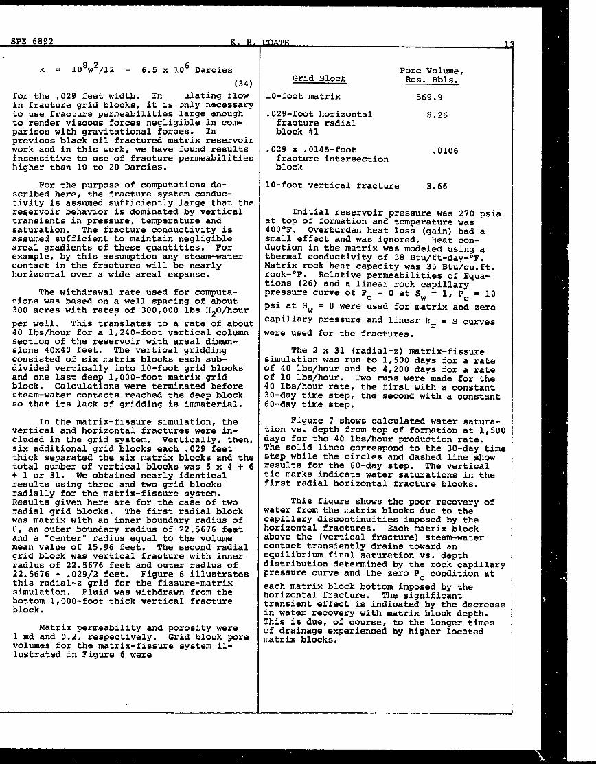
In the matrix-fissure simulation, thevertical and horizontal fractures were in-cluded in the grid system. Vertically, then,six additional grid blocks each .029 feetthick separated the six matrix blocks and thetotal number of vertical blocks was 6 x 4 + 6+ 1 or 31. We obtained nearly identicalresults using three and two grid blocksradially for the matrix-fissure system.Results given here are for the case of tworadial grid blocks. The first radial blockwas matrix with an inner boundary radius ofO, an outer boundary radius of 22.5676 feetand a “center” radius equal to the volumemean value of 15.96 feet. The second radialgrid block was vertical fracture with innerradius of 22.5676 feet and outer radius of22.5676 + .029/2 feet. Figure 6 illustratesthis radial-z grid for the fissure-matrixsimulation. Fluid was withdrawn from thebottom 1,000-foot thick vertical fractureblock.

Matrix permeability and porosity were1 md and 0.2, respectively. Grid block porevolumes for the matrix-fissure system il-lustrated in Figure 6 were

Pore Volume,Grid Block Res. Bbls .

10-foot matrix 569.9

.029-foot horizontal 8.26fracture radialblock #1

.029 X .0145-foot .0106fracture intersectionblock

10-foot vertical fracture 3.66

Initial reservoir pressure was 270 psiaat top of formation and temperature was400”F. Overburden heat loss (gain) had asmall effect and was ignored. Heat con-duction in the matrix was modeled using athermal conductivity of 38 Btu/ft-day-°F.Matrix rock heat capacity was 35 Btu/cu.ft.rock-°F. Relative perrneabilities of Equa-tions (26) and a linear rock capillarypressure curve of Pc = O at SW = 1, pc = 10

psi at Sw = O were used for matrix and zero

capillary pressure and linear kr = S curves

were used for the fractures.

The 2 x 31 (radial-z) matrix-fissuresimulation was run to 1,500 days for a rateof 40 lbs/hour and to 4,200 days for a rateof 10 lbs/hour. Two runs were made for the40 lbs/hour rate, the first with a constant30-day time step, the second with a constant60-day time step.

Figure 7 shows calculated water satura-tion vs. depth from top of forqation at 1,500days for the 40 lbs/hour production rate.‘l’hesolid lines correspond to the 30-day timestep while the circles and dashed line showresults for the 60-day step. The verticaltic marks indicate water saturations in thefirst radial horizontal fracture blocks.

This figure shows the poor recovery ofwater from the matrix blocks due to thecapillary discontinuities imposed by thehorizontal fractures. Each matrix blockabove the (vertical fracture) steam-watercontact transiently drains toward anequilibrium final saturation vs. depthdistribution determined by the rock capillarypressure curve and the zero Pc condition at

each matrix block bottom imposed by thehorizontal fracture. The significanttransient effect is indicated by the decreasein water recovery with matrix block depth.Phis is due, of course, to the longer timesof drainage experienced by higher locatedmatrix blocks.

,4 GEOTHERMAL RESER

The horizontal fracture blocks opFositethe 100% steam saturhted vertical fracturegrid blocks rapidly r~se toward 100% steamsaturation. Above the steam-water contact,the water draining from the bottom of amatrix block enters the i~orizontal fractureblock and then preferentially flows vertical-ly down into the top of the next lower matrixblock rather than laterally into the verticalfracture. This preference is very close to100%. These latter results are shown bymodel printouts of Watfi,rznd steam interlockflow rate macjnitudes and directions atselected times.

Table 7 summarizes averaqe iterationsper time step, average saturation change~maximum over grid) per time step and com-puting times for the three fL_FiCtUred-rnatrixSimulation runs. The negligible time trunca-tion error for 30- and 60-day time stepsshown in ?igure 7 is somewhat surprising inlight of the average saturation change risingfrom .;?~for t;:e30-day step to .66 for the60-da! ste~. The .66 figure is actuallyconscr”~ative~ince 27 vertical fracture gridblocks were swept from O to 100% steamsaturation in only 25 steps in Run 2. Notime steps were repeated due to divergence inmy of these runs in spite of nearly 100%;aturation chanqes in one step for the .01 R13?ore volume fracture-intersection grid blocks3oth Runs 1 a]ld2 .x~erienced a number ofLime steps of 90-100% saturation change.Vo.

Run1 computing time corresponds to a time

?er block-step of about .01 seconds.

Figure 8 compares the effect of produc-ing rate on matrix-fissure simulation resultsPhe calculated sa~urations for Run 1 at 40lbs/hour and Run 3 at 10 lbs/hour are com->ared at times cf equ~l cumulative produc-:iQn. The steam-water contact for the higher:ate is 40% (140 feet VS. 101 feet) deeperIue to the shorter time available for:ransient water drainage from the matrix)locks above the contact.

(conventional simulation results were]enerated by running the model in one-Iimensional vertical mode using 24 10-foot)locks and one lrOOO-foot block. The dashed.ine in Figure 9 shows resulting calculatedlater saturation vs. depth at 1,500 days form “effective” permeability of 50 md and amoducing rate of 40 lbs/hour. Gravity;orces dominate and the conventional results;how a sharp transition zone from a drained:Sw=swc= .2) upper region to the 100% water

zone. The transition zone is considerablyligher than the matrix-fissure simulationresults viewing either the matrix or theJertical fracture steam-water contact.

‘OIR MODELLING SPE 68

We can achieve somewhat greater realismin the conventional simulation by utilizingthe fact that the capillary discontinuitieseach 40 feet impose a maximum final recoveryof water (by flow alone) which can be pre-determined using the rock capillary pressurecurve, the 40-foot matrix block height andthe .369 psi/foot water-steam density(gradient) difference. Following Reference[81 we integrate the S - p= relation over

wthe 40 feet using the fact that Pc = O at

matrix block bottom and find that finalminimum average matrix block water saturationis .417. Using this value for Swc in the

relative permeability equations, the con-ventional simulation Sives the water satura-tion profile indicated by the larger dashedllne in Figure 9.

Further adjustments in various datamight be made to narrow the differencebetween matrix-fissure and conventionalsimulation results. Considering the basicdifference in mechanisms for the conventionaland more correct matrix-fissure calculations,we hold little hope for forcing accuracy froma conventional simulation. In particular,the above described rate effect (Figure 8)is shown by the more rigorous matrix-fissuresimulation, but not by conventional simula-tion (unless the permeability used is verylow).

A full three-dimensional simulation of afractured-matrix reservoir will require tyincrin this vertical two-dimensional RIZ matr~x--fissure calculation.to a two-dimensionalsreal calculation w.lerethe areal blockscormnunicatethrouq;,the fracture system andthe interlock flows reflect the different“sector” or areal ~lock steam-water contacts.rhis task will involve a significant effortin locjicand coding and will in many casesrequire disking on fixed memory machines.rhe two-dimensional R-Z matrix-fissurecalculation described here is adequate onlyif the areal gradients within the reservoiraxe assumed small due to high fractureconductivity.

Interpretation of Pressure Drawdown Tests

The major differences between conven-tional and matrix-fissure simulation resultsjust described arose because of the two-phaseE1OW in a system having capillary discon-tinuities. Here we illustrate difficultieswhich can arise in using conventional simula-tion to interpret pressure drawdown tests infractured-matrix, hot water systems withsingle-phase water flow.

Simulation of a well test in a systemhaving a three-dimensional network of or-thogonal fracture planes would require a fullthree-dimensional Cartesian grid. To sim-plify for the purpose of illustration, weconsider a system of 44-foot matrix layersseparated by ho~izontal fractures. A 10x5radial-z grid was used to model a horizontaldisk of matrix beneath a horizontal fracture.The disk dimensions were exterior radius re =10,000 feet and thickness = 22 feet. Thefive layer thicknesses were J/2, 2, 4, 8, 8feet where w is horizontal fracture thick-ness. This disk is a symmetrical element forthe case where the well penetrates the entireformation thickness.

The radial spacing was calculated usingEquation (29) with the wellbore included inthe grid. Wellbore radius was .25 and the 10block “center” radii were .25, .43, l~3&,4.48, 14.55, . . ., 5,242.37 feet. Porevolumes of the tiellborecells varied from.000014 to .2798 RB in layers 1-5 for a smallfracture width w = .245 mm.

Matrix and fracture layer porositieswere .2 and 1.0, respectively. Initialtemperature was uniformly 350”F and initialpressure was 2800 psia at top of formation.The illustrative pressure drawdown testconsisted of producing 10,000 lbs/hour from awell open in all five layers for ten days.Fracture conductivity and matrix permeabilitywere varied in five simulation runs astabulated in Figure 10. The fracture perme-abilities were related to fracture width by

the relationship k = 108w2/12 where k is inDarcies and w in cm. The homogeneous (nofracture) case, Run 4, has a permeability of90.9 md, which gives a total md-ft productfor the 22-foot thicfinessequal ~o that ofthe fracture cases.

Figure 10 shows calculated pressuredrawdown (initial pressure-flowing wellborepressure) vs. time on a semi-log plot forfive cases. The homogeneous case (Run 4)gives a straight-line and use of the well-known relationship, slope = Qu/4wkh, givesk = 90.9 md, in agreement with the valueused. Arbitrary use of the average slopefrom .1 to 1 days with the relation slope =Q1.i/4nkhgives k = 247, 188 and 157 rndforRuns 1-3, respectively. These permeabilitiesbear little resemblance to either fracture ormatrix permeabilities.

The semi-log plots of pressure drawdownVS. time actually are not linear ior thefracture cases, but are rather.concave up-ward. This results from the fact that thereservoir transient is primarily a crossflow(vertical) bleeding of fluid into the frac-ture rather than the radial transient of ahomogeneous unfractured formation. Thedegree of upward curvature of the drawdowncurve increases as matrix permeabilitydecreases.

The cases of small fracture width, Runs1-3, exhibit a rapid initial drawdown of 60-80 psia in the first few minutes of flow.The calculated effect of a fivefold largerfracture width is one of reducing this earlydrawdown to 2-3 psi. However, for timesafter the first few minutes, the largerfracture gives a calculated, concave upwarddrawdown curve of shape virtually identicalto that for the smaller fracture. This isillustrated by the curves for Runs 1 and 5 inFigure 10.

Figure 11 shows calculated drawdowns fora tenfold larger horizontal fracture spacingof 440 feet. The simulations used a 10 x 8grid with the eight layer thicknesses equalto .0004, 2, 4, 8, 16, 32, 64 and 94 feet (atotal thickness of 220 feet). The kw productfor the total fracture width of .0008 feet(.245 mm) is 4 Darcy-feet. A drawdown testflow rate of 100,000 lbs/hour was specified.The curve for this Run 6 in Figure 11 shows al!learity of drawdown vs. In(t) past 10 daysto about 30 days. The upward concave curveshape from 100 to 1,000 days is due toestablishment of semi-steady-state conditionsthroughout the reservoir.

The curve labeled Run 7 in Figure 11 wascalculated for a 220-foot homogeneous res-ervoir with k = 9.09 md corresponding to anequivalent total red-feetproduct of 2,000.The slopes of the curves for Runs 6 and 7 onFigure 11 give formation permeabillties of 18md and 9.09 md, respectively. If the 10-daytest portion of the Run 6 curve were analyzedby conventional radial flow theory, then apermeability of 18 rndand a skin factor of9.65 would be determined. The circles of Run8 in Figure 11 show the simulator results fora homogeneous reservoir with this perme-ability and skin factor. Figure 11 showsthat calculated drawdowns for the fracturedformation (Run 6) and for an 18 md, homoge-neous formation with skin (Run 8) agree wellthrough 1,000 days.

These results of Figure 11 indictitethatfor the particular fracture spacing and widthof 440 feet and .245’mm, respectively, con-ventional radial flow analysis wotlld (a)yield erroneous permeability and skin but (b)give accurate long-term deliverability predic-tions. This conclusion does not hold for thepreviously discussed results of Figure 10corresponding to the smaller fracture spacingof 44 feet. For ::.Lsspacing, the short-termdrawdown test can fail to yield any linearityfrom which conventional analysis candetermine effective permeability and skin.

Several additional complexities that mayexist in practice need mentioning in con-nection with the resulks just discussed. Anaturally fractured formation will generallyhave vertical as well as horizontal frac-tures. Accounting for a three-dimensionalnetwork of fracture planes with the model

16 GEOTHERMAL RESERVOIR MODELLING SPE 6892

described herein would require a three- HEAT EXTWCTION FROM HOT DRY ROCK

dimensional simulation. If fracture spacingwere the order of 100 feet or less, a verylarge number of grid blocks would be re-quired. A better modelling approach in this We consider a vertical fracture in a hotcase would be a dual porosity formulation dry rock initially at 500°F. A 5x5x5 three-where interlock flow is assumed to occur dimensional grid describes a rectangularonly in the fracture system. The matrix parallelepipedswith Ax = Az = 80 feet andwould be accc’.mted for by zero-dimensional, Ay = .01, 30, 120, 160, 320. These dimen-one-dimensional spherical or two-dimensional sions resulted from combining blocks in acylindrical subcal~dlations tied into the comparison run which used y-direction in-fracture porosity in each grid block. The crements of .01, 10, 20, 40, 80, 160 and 320heat-loss calculation described in Reference feet. The overall dimensions are a 400x400-

[31 is an example of this type of formulation. foot vertical crack of .02-foot width with630 feet of rock either side of it. The

The model described here may apply well 630 feet of rock in the y-direction isto an artificially fractured formation since sufficiently large that the system acts asin this case the vertical fractures will infinite for the 3,000 days of simulation.intersect the well. linr-0-z grid rep- Different grids were used to determine theresenting a symmetrical element in this case acceptably low spatial truncation error ofmay accurately model well performance with the 5x5x5 grid.a reasonably low number of grid blocks.

Since the system is symmetrical aboutAn upward concave deviation from the vertical midplane of the crack, this

linearity in a drawdown test curve may result 5x5x5 grid represents half the system. Crackfrom factors other than formation fractures. width is of no consequence except in itsGeothermal reservoirs with brines of high relation to the kw product where k is frac-salinity may precipitate salt with pressure ture permeability and w is fracture totaldrawdown near the well. This can cause a width. In the grid plane j = 1 (the crack)skin factor increasing with time and the an x-z thermal conductivity of 3.8 Btu/ft-mentioned deviation from linearity. It is dav-°F was used, porosity was 1.0 andwell-known that faults or other flow bar- permeability was varied over a number of runsriers near a well can cause upward curvature. from 10 Darcies to 800,000 Darcies. In theShort-term drawdown tests on wells which planes, j = 2-5 (hard rock) thermal con-partially penetrate thick formations, ductivity was 38 Btu/ft-day-°F, rock specificespecially where the ratio of vertical to heat was 35 Btu/cu.ft.rock-°F and porosityhorizontal permeability is small, can result and permeability were zero.in deviation from linearity. Regardless ofpenetration, a formation consisting of 100°F cold water injection rate wasalternating tight and permeable streaks of specified as 25,000 lbs/hour into the bottomlarge permeability contrast can yield devia- left corner of the crack (cell i=l,j=l,k=5).tion from linearity through the same ver- A withdrawal well at the upper right cornertical, crossflow type of transient treated of the crack (cell i=5,j=l,k=l) maintainedabove in the horizontally fractured formation pressure at 800 psia due to a iarge specifiedcalculations. Quoting from Reference [111, productivity index. This withdrawal wellwhich treated simulation of single-phase gas produced on deliverability against the 800flow, “. . . The reservoir picture finally psia pressure. The 25,000 lbs/hour injectionemployed with success stemmed from the rate corresponds to actual injection wellhypothesis that the well communicated with a rate of 50,000 lbs/hour since the gridnumber of thin permeable stringers . . . fed represents a symmetrical half of the totalby severely limited crossflow from large system.sand volumes. . . .“. In that work, for suchreservoirs, the calculated and observed Figure 12 shows calculated energydrawdown/buildup curves failed to yield the recovery and prodncing well bottomholelinearity of conventional analy:3is. temperature.vs. time. Energy recovery is

defined as cumulative enthalpy producedFinally, the fractured formation, draw- divided by the sensible heat above 100’F

~own test illustrative calculations and initially contained in a portion of the rock.interpretations presented here are not unique The portion used is the first 310 feet sinceto geothermal reservoirs, but apply to any the last 320 feet experienced essentially noformation subject to single-phase flow of a recovery (temperature decline) at 3,000 days.low compressibility fluid -- oil, water or The initial energy in place on these bases is

high pressure gas. 6.944 X 1011 Btu. Enthalpy of produced wateris U + pv where internal energy U is zero at100°F.

CDF &QQ9 K. 1-1-f!13AWS 17

.

.

Figure 12 shows a rapid decline ofproduced water temperature from 500”F toless than 300”F in the first few days fol-lowed by a very flat decline from 170*F to137°F from 1,000 to 3,000 days. Fractionalenergy recovery is 0,1663 at 3,000 days,..equivalent to 1.155 x 10IL Btu or an averageof 64 Btu/lb water produced (enthalpy rela-tive to zero U at 100°F). The average tem-perature corresponding to this averageenthalpy is about 162°F.

The fracture width w controls systemconductivity or throughput. The corre-sponding parameter or group of importanceis the kw Darcy-feet product, which is

proportional to W3 since fracture perme-

ability is proportional to Wz. We usedpermeabilities up to 800,000 Darcies withthe .02-foot model dimension for thefracture. This 16,000 Darcy-foot kwproduct corresponds to a fracture widthof 4 mm using the fracture permeability

equation k = 108w2/12 (w in cm). Fracturewidth, i.e. the kw product, had no effecton the calculated recovery and temperatureshown in Figure 12.

Model runs were made with the injec-tion well located higher, 200 feet fromtop of formation in cell i=l,j=l,k=3. Thechange of injectiop location had no effecton calculated recovery and producingtemperature.

Figure 12 also shows calculated re-covery and temperature for a larger frac-ture of dimension 800x800 fee$. Again,the above described kw product and injec-tion well location variations had-noeffect on the calculated recovery andproducing temperature. The larger frac-ture resulted in a considerably higherbottomhole producing temperature vs. timeand a lower fractional energy recovery.Calculated absolute energy recovery at3,000 days was higher for the larger

fracture -- 3.53 x 1011 Btu VS. 1.15:h5X~01LBtu for the 400x400 foot fracture.a fourfold increase in fracture area causeda threefold increase in energy recovery.Average enthalpy of produced water was196 Btu/lb corresponding to an average“temperature of produced water of 292”F.

The runs were performed using automatictime step control due to the rapid initialtransients. With a first time step of .1days, a subsequent minimum At of .2 days,control by 150°F maximum grid block tem-per~ture change per time step and amaximmn time step of 500 days, the modeltook 13 time steps to 3,000 days fsc the100,00(,Darcy permeability. CompJter timefor this run was 46 CDC 6600 CPU seconds.Twenty of these seconds were required forthe first two time steps.

Calculated results for permeabilitiesless than 100,000 Darcies exhibited nocirculatory “free” convection type cellsin the vertical fracture plane. Table 8shows an example of these results at3,000 days for the case of a 400x40Qfoot fracture, and 100,000 Darcies frac-ture permeability which corresponds to a2 mm frac’turewidth. The table showscalculated pressures in the fracture plane,temperatures in all planes and interlockflow rates (positive to the right andvertically downward). Water flow isuniformly to the right and upwards away fzomthe injection in grid cell i=l,j=l,k=5. Tem-perature uniformly increases to the right andupward (in the directions of water flow)except in the top row.

Results for the 800,000 Darcy perme-ability differed markedly from those justdescribed. Table 9 shows pressure, tem-perature and flow rate distributions at 75days for the 800x800 foot fracture with800,000 Darcies. y-direction spacin,-wasaltered in this run to .01, 10, 30, 50, 180feet. The flow rates in Table 9 show ex-tremely strong “free” convection cells in the5x5 grid of the vertical fracture plane.Water is in fact flowing downward into theinjecting cell i=l,j=l,k=5. The flow dis-tribution is complex and the temperaturechange from left to right alternates in signin alternate rows corresponding to alterna-tion in direction of horizontal flow rate.

Table 10 shows pressure, temperature andflow rate distributions for this 800,000Darcy case at 3,000 days. While the flowrates are much more uniform with flowuniformlv upward, the free convection stillexists with some horizontal flow from rightto left. Deviations from a pattern of uni-form temperature increase to the right andupward are small but exist and are complex.This 800,000 Darcy run was much more dif-ficult than the runs for 100,000 or fewerDarcies. The number of time steps increasedto 21 and computer time increased to 144 CDC6600 CPU seconds, largely due to divergenceand repeat of one of the time steps.

These fractured hot rock simulations didnot employ any enhanced heat conduction tothe fracture due to thermal cracking inducedby temperature decrease. A functional re-lationship between thermal conductivity andtemperature or temperature change can beincluded in the model. Such a relationshipand associated parameters might be deducedfrom laboratory or field e~perimental data.

L ti UYJYJ~ -. lx.B~w Vrzl Uo>d

SUMMARY A limited investigation of time trunca-tion error indicates that acceptably lowlevels can occur in spite of average maximum

An implicit, thzee-dimensional gee’(over grid) saturation changes per time

:hermal model is describlxland partiallystep as high as 60%.

waluated in respect to stability or timestep tolerance. The model is only partlyimplicit in certain applications whererarious terms associated with allocation ofJell rates among open layers are treated:xpliclLly. NOMENCLATURE

The implicit model stably accommodated:ime steps corresponding to 80-100% satura-tion change in a grid block and throughput A cross-sectional area normal to

catios the order of 108 in several illustra- flow, ft2:ive multiphase flow problems. This compares~ith our experience of limits of 3-10% c compressibility, l/psisaturation change and throughput ratio ofroughly 20,000 with semi-implicit geothermal Cp specific heat, Btu/lb-°Fmd oil reservoir models. The implicit modelstability allowed inclusion of fractures and (PCP:R rock specific heat, Btu/cu.ft rock-°Frellbores as small-volume grid blocks in~everal multiphase flow test problems. fw water phase volumetric fractional

flowAn analytical derivation is presented

~or a well deliverability reduction factor fg gas phase volumetric fractional flowthich can be used in simulations using largelrid blocks. The factor accounts for in- f well.deliverability factor, fraction:reased pressure drop near the well due tolot water flashing and steam expansion. H enthalpy, U + pv, Btu/lb

The model was used to simulate two-phase k absolute permeability, mdlepletion of a fractured matrix reservoir~ith horizontal and vertical fractures in- kr:luded as grid blocks.

relative permeability, fractionThe results were

>oorly matched by conventional simulation k relative permeability to gas atrhich treats the reservoir as an unfractured rgcw

irreducible water saturation SFormation with high effective permeability. Wc

K thermal conductivity, Btu/ft-day-°FSimulation of a single-phase flow,

xessure drawdown test in a tight formation NX,NY,NZnumbers of grid blocks in reservoirvith horizontal fractures showed upward con- grid system, in x, y, z directions,:ave curvature of the pressure drawdown vs.in(t) plot.

respectivelyThe degree of calculated cur-

rature and attendant interpretation dif- G desired or target production rate,Ficulty increased with decreasing matrix lbs H20/daypermeability level and decreasing horizontal?racture spacing. q production rate, lbs H20/day

The final illustrative application qH enthalpy production rate, Btu,lday:reated heat extraction from a fractured, hotIry rock system. For a given cold water qHL heat loss rate, Btu/dayinjection rate, the calculated energyrecovery and production well water tem- PS (T) water vapor pressure>erature vs. time were not affected by:racture permeability-width product or in- P gas phase pressure, psiaiection well location. The fracture con-ductance was varied from 2 to 16,000 Darcy- pwb wellbore flowing pressure, psiait, while injection well location was variedmly from the bottom corner to the mid-depth pc capillary pressure, p~f the fracture plane. A fourfold increase 9

- pw, psi

in fracture area from 400x400 to 800x800% throughput ratio, Equation (31)

square feet resulted in a threefolt increasein calculated energy recovery at 3,000 days r radius, feetfor the same cold water injection rate.

SPE 6892 K. H . C!OATS .,

—

—

—-— ---— . . . .. ---- --- L!

re exterior radius T= reservoir heat conduction trans-missibility KA/k, where k =

rw wellbore radius distance between grid blockcenters, Btu/day-OJ?

RB Reservoir BarrelsT gas phase transmissibility,

s skin factor 9 (kA/!WcrgPg/pg) X .00633,

Sw water phase saturation, fraction lbs gas phase/day-psi

s gas phase saturation, fraction Tw water phase transmissibility,~ (kA/LZ)(krwPw/vw)X .00633,

sge gas saturation at r = re lbs water phase/day-psi

sWc irreducible water saturation A(TAP) = Ax(TxAxp) + Ay(TyAyp) + Az(TzAzp),

s critical gas saturation defined as indicated abovegc Equation (5)t time, days

P viscosity, cpAt time step, tn+l - tn, days

r temperature, “F SU3SCRIPT’S +..

r5 :;ter saturation temperature, Ts(p), e exterior

~ gas (steam) ~haseJ internal energy, Btu/lb

i,j,k grid block ind~hqi,yj,zkJP

grid block pore volume, V(Ik grid layer number or index .

J grid block bulk volume, AxAYAz,cubic feet 1 (superscript) iteration number

J specific volume, cu.ft/lb n time level, tn

~ fraction width s saturation condition

< quality, mass fraction steam X,y)z denotes x, y or z direction,respectively

<,y,z Cartesian coordinates, feet, zmeasured positively vertically w water phasedownward

wb wellbore\x,Ay,Az grid block dimensions, feet

;REEKREFERENCES

r)

1. Coats, K. H., and Ramesh, A. B.,“Numerical Modeling of ThermalReservoir Behavior”, Preprint presented

i at the 28th Armual Technical Meetingof the Petroleum Society of C.I.M.,Edmonton, Alberta, May 27-June 6,1977. “

)2. Carterl R. D., and Tracy, G. W.,

) “An Improved Method for CalculatingWater Influx”, Trans. AIME (1960),

r 219, 415-417.

3. COat5~ K. H., George, W. D., Chu,1 Chieh, and Marcum, B. E“.,“Three-

Dimensional Simulation of Steamflood-ing”, Trans. AIME (1974), 257, 573.

time difference operator,

Xx=x n+l - ‘n

iteration difference operator,

ax ~ x~+l - xl

porosity, fraction

density, lbs/cu.ft

specific weight or gradient,psi/ft (yw = p/144)

mobility, kr/~

=. “-” --------- .-”-.. . . . . . ‘-4” -- A.I-A.. W “.- ““a

4. Toronyi, R. M., and Ali, .S.M. Farouq, = 2nkAz ~p ‘Wpw“Two-phase, Two-Dimensional Simulation q— — dp

ln> pwb l-x(36)

of a Gc.othermalReservoir”, Sot. Pet.Eng. J. (June, 1977), 171-183. w

5.or

Blair, P. M., and Weinaug, C. F.,“Solution of Two-Phase Flow Problems

= :* l(p~p~b~sg)Using Implicit Difference Equations”, q (37)

Trans. AIME (1969), 246, 417. q

6. PriCe? H. S., and Ceats, K. H.r“Direct Method in Reservoir Simula- where the integral I is a function only oftion”, Trans. AIME (1974), 257, 295. the integration limits pwb,P ana of steam

7. Steam Tables, Keenan, J. H., and saturation Sg at R bzcause, as we will now

Keyes, F. G., Hill, P. G., and show, the integrand Awpw/(l-X) is a .single-Moore, J. G.t John Wiley & Sons,1969. valued calculable function of pressure p.

3. COat5, K. H., Nielsent R. L., Flowing quality X is related to frac-

Terhuner M. H., and Weber, A. G., tional flow by

“simulation of Three-DimensionalTwo-Phase Flow in Oil and GasReservoirs”, Sot. Pet. Eng. J. x= 1/(1 + fwpw/(l-fw)Pg) (38)

(December, 1967), 377-388.

3. Coats, K. H., Dempsey, J. R., and and enthalpy per lb of flowing stream is

Henderson, J. H., “The Use ofVertical Equilibrium in Two-DimensionalSimulation of Three-Dimensional Res- H = XH9 + (1 - X)HW (39)

ervoir Performance”, Trans. AIME (1971),251, 63-71.—. At steady-state, fiowing stream enthalpy is

LO. Flow of Homogeneous Fluids, Muskat, M., constant and from (39),

J. W. Edwards, Ann Arbor, Michigan,1946.

x = (H--Hw]/(Hg-Hw) = X(P), (40)

il..,Coats, K. H., Dempsey, J. R., Ancell,‘R. L., and Gibbs, D. E. , “Analysisand ‘?Kqdiction of Gas Well Performance”, where the dependence upon pressure alone

SPE 3474 presented at 46th Arnnual follows from the fact that H is constant and

Meeting of ~~, New Orleans, Louisiana., saturated water and steam enthalpies are

October 3-6, S.971. single-va. ‘ed functions of pressure. FromEquation (..~, .

APPENDIX fw = 1/!1 + xp#(l - X)pgl = fw(p)

CALCULATION OF DELIVERABILITY FACTOR f. (41)

We consider two-phase, steady-statewhere the dependence upon pressure alonefollows from *he fact that saturated water

steam-water flow from some exterior radius Rto wellbore radius rw.

and steam densities are single-valuedThe point R is functions of pressure.

assumed to be saturated, and pressure is P at If p and S at R are given, then9R and pwb at rw.

Darcy’s law givtisliquid water phaseenthalpy H can be calculated from Equations

flow rate at any radius as(38) and (39). Given H, we can calculatethe values of X(p) and fw(p) at any pressure

from Equations (40) and (41). Thus, the

qw =q(l-x)= -2~kAzAwpwrdp/dr (35) integral in Equation (36) can be numericallyintegrated for any given values of P, pwb ands9“

where X is flowing steam quality, q is totalflow rate, lbs H20/day, kAz is md-ft product

x .00633, Aw is k~/uw and Pw is water den-

sity in lbs/cu.ft. Integration using thefact that q is constant gives

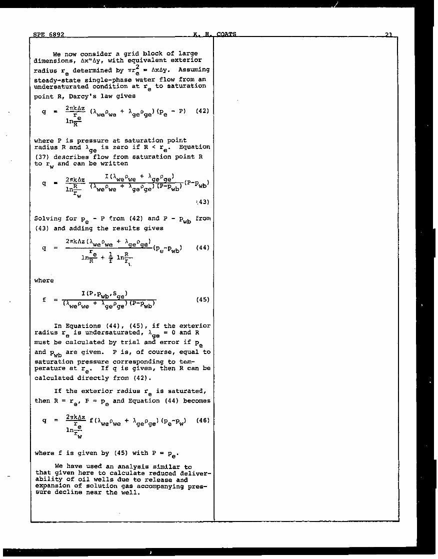
2~G 007#Z

We now consider a grid block of largedimensions, Ax=Ay, with equivalent exterior

radius re determined by @ = AxAY. Assuin9

steady-state single-phase water flow from anundersaturated condition at re to saturation

point R, Darcy’s law gives

q= + (Avjepwei-AgePge)(pe - P) (42)

ln$

where P is pressure at saturation poir,tradius R and X is zero if R < re. Equation

(37) describesg~low from saturation point Rto rw and can be written

2nkAz I(Awepwe + a ep e)q=— (p-pwb)

ln> ‘~+

we ‘we ‘ge~ge)(p-pwb)

w1,43)

Solving for pe - P from (42) and P - pwb from

(43) and adding the results gives

2mkAz(Awepwe + A ep e)q = (pe-pwb) (44)

ln~ + * In%s.

where

I(p,pwb,S e)f =

( +a (45)‘we‘we gepge) (‘-pwb)

In Equations (44), (45), if ~h~ eX~~iOrradius r= is ufidersaturated, Agemust be calculated by trial and error if pe

and pwb are given. P is, of course, equal to

saturation pressure corresponding to tem-perature at re. If q is given, then R can be

calculated directly from (42).

If the exterior radius re is saturated,

then R = re, F = pe and Equation (44) becomes

2rkAzq= — f(awepwe + ‘ge~ge) ‘Pe-pw) (46)

ln~w

where f is given by (45) with P = pe.

We have used an analysis similar tothat given here to calculate reduced deliver-ability of oil wells due to release andexpansion of solution gas accompanying pres-sure decline near the well.

—

—

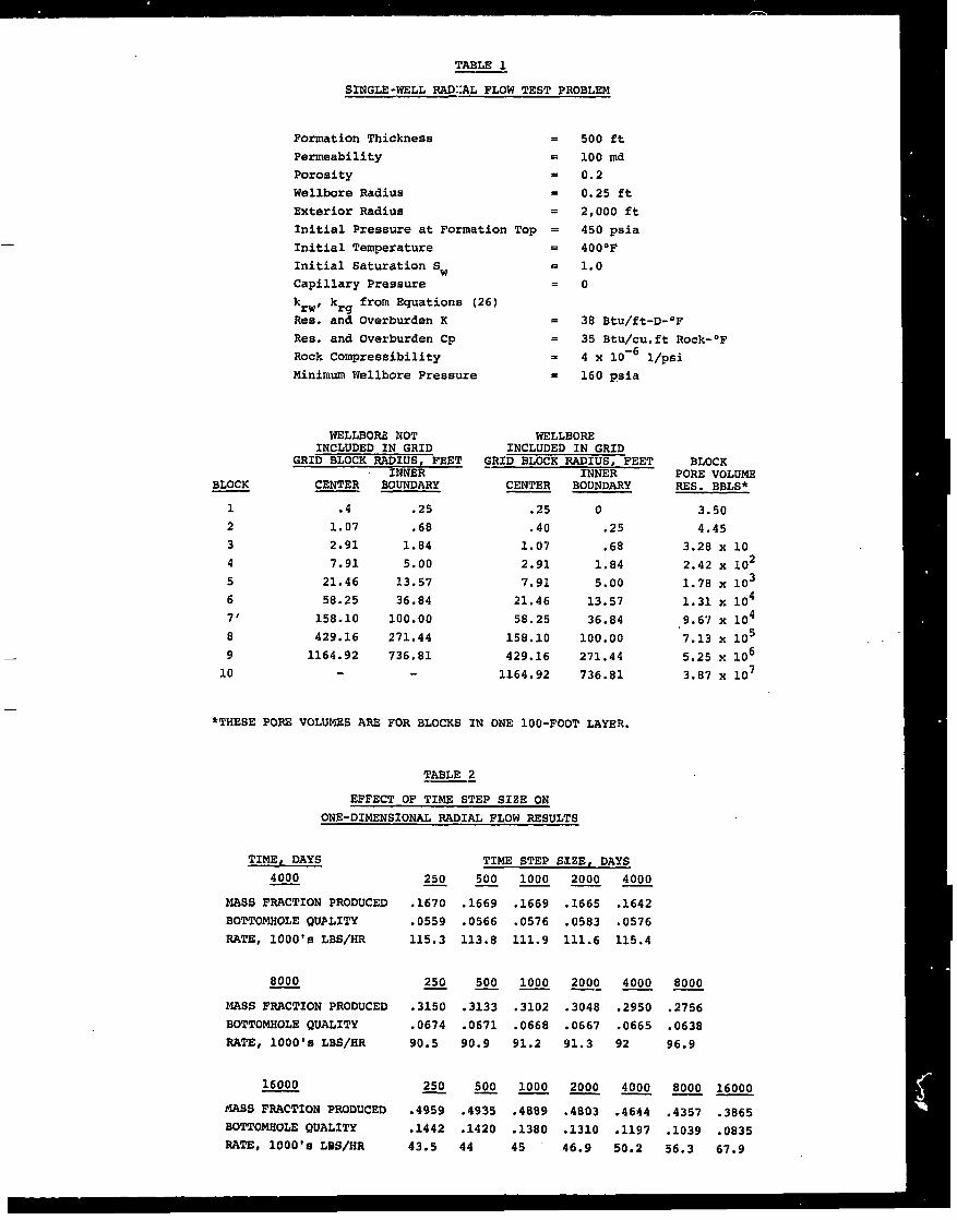
1

2

3

45

67’

8

910

TABLE 1

PermeabilityPorosityWellboreRadius

Exterior Radius

Initial Pressure at Formation

Initial Temperature

Initial Saturation Sw

Capillary Pressure

k , krg from Equations (26)

R~;. and Overburden X

Res. and Overburden Cp

Rock Compressibility

=E

.

.

TOP =

=

.

.

.

.=

100 md

0.2

0.25 ft2,000ft450 psia400”F1.0

0

38 Btu/ft-D-”F

35 Btu/cu.ftRock-°F4 x 10-6 l/psi

Minimum Wellbore Pressure . 160 psia

WELLBORENOTINCLUDEDIN GRID

GRID BLOCKRADIUS,FEETINNER

CENTER BOUNDARY

.4

1.07

2.917.91

21.4658.25

158.10429.16

1164.92

.25

.68

1.84

5.00

13.57

36.84

100.00

271.44

736.81

SINGLE-WELL RAD::AL FLOW TEST PROBLEM——

Formation Thickness . 500 ft

lWS. BBLS*

“7.13 x 105

8000

8000 16000——

WELLBOREINCLUDED IN GRID

~RID BLOCK RADIUS, FEETINNER

CENTER

.25

.40

1.07

2.91

7.91

21.46

58.25

158.10

429.16

1164.92

BOUNDARY

o

.25

.68

1.s4

5.00

13.57

36.84

100.00

271.44

736.81

*THESE PO$E VOLUMES ARE FOR BLOCKS IN ONE 1OO-FOOT LAYER.

TABLE 2—.

EFFECT OF TIME STEP SIZE ON

ONE-DIMENSIONAL RADIAL FLOW RESULTS

TINE, DAYS

4000

MASS FRACTION PRODUCED

BOTTOMHOLE QU?LITY

RATE, 1000’s LBS/HR

8000

MASS FRACTION PRODUCED

BOTTOMHOLE QUALITY

RATE, 1000’s LBS/HR

16000

MASS FRACTION PRODUCED

BOTTOMHOLE QUALXTY

RATE, 1000’s LBS/HR

250

.1670

.0559

115.3

250

.3150

.0674

90.5

250

.4959

.1442

43.5

TIME STEP SXZE, DAYS

500 1000 2000 4000—— ——

.1669 .1669 .1665 .1642

.0566 .0576 .0583 .05~6

113.8 111.9 111.6 115.4

500 1000 2000 4000—— —-—

.3133 .3102 .3048 .2950

.0671 .0668 .0667 .0665

90.9 91.2 91.3 92

500 1000 2000 4000—— —_

.4935 .4889 .4803 .4644

.1420 .1380 .1310 .1197

44 45 46.9 50.2

BLOCKPORE VOLUME

3.50

4.45

3.28 X 10

2.42 X 102

1.78 X 103

1.31 x 104

9.6”1X 104

5.25 X 106

3.87 X 107 I

.2756

.0638

96.9 I.4357 .3865

.1039 .0835

56.3 67.9

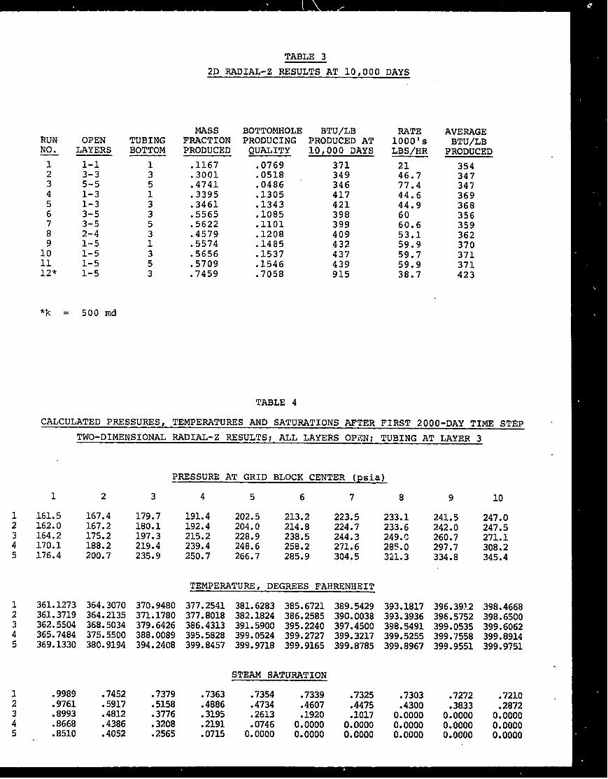
TABLE 3

2D RADIAL-Z RESULTS AT 10,000 DAYS

12

:5

12345

12

:5

RUNNO.

123456789

101112*

OPENLAYERS

1-1

::;1-31-33-5

:::1-51-51-51-5

TUBINGBOTTOM

1351335

?353

MAssFIU%CTIONPRODUCED

.1167,3001.47413395:3461.5565.5622.4579.5574.5656.5709.7459

BOTTOMHOLE BTU/LBPRODUCING PRODUCED ATQUALITY 10,000 i)AYS

.0769 371

.0518 349

.0486 346

.1305 417

.1343 421

.1085 398

.1101 399

.1208 409

.1485 432

.1537 437

.1546 439

.7058 915

WTE1000’sLBS/HR

2146.777.444.644.96060.653.159.959.759.938.7

AVERAGEBTU/LB

PRODUCED

354347347369368356359362370371371423

*k = 500 rnd

TABLE 4

CALCULATED PRESSURES, TEMPERATURES AND SATURATIONS AFTER FIRST 2000-DAY TIME STEP

TWO-DIMENSIONAL RADIAL-Z RESULTS; ALL LAYERS OPEN; TUBING AT LAYER 3

PRESSURE AT GRID BLOCK CENTER (psia)

1 2 3 4 5 6 7 8 9 10

161.5 167.4 179.7 191.4 202.5 213.2 223.5 233.1 241.5 247.0162.0 167.2 180.1 192.4 204.0 214.8 224.7 233.6 242.0 247.5164.2 175.2 197.3 215.2 228.9 238.5 244.3 249.C 260.7 271.1170.1 188.2 219.4 239.4 248.6 258.2 271.6 28~00 297.7 308.2176.4 200.7 235.9 250.7 266.7 285.9 304.5 321.3 334.8 345.4

TEMPERATURE, DEGREES FAHRENHEIT

361.1273 364.3070 370.9480 377.2541 381.6283 385.6721 389.5429 393.1817 396.39?.2398.4668361.3719 364.2135 371.1780 377.8018 382.1824 386.2585 390.0038 393.3936 396.5752 398.6500362.5504 368.5034 379.6426 386.4313 391.5900 395.2240 397.4500 398.5491 399.0535 399.6062365.7484 375.5500 388.0089 395.5828 399.0524 399.2727 399.3217 399.5255 399.7558 399.8914369.1330 380.9194 394.2408 399.8457 399.9718 399.9165 399.8785 399.8967 399.9551 399.9751

STEAM SATURATION

.9989 .7452 .7379 .7363 .7354 .7339 .7325 .7303 .7272 .7210 .

.9761 .5917 .5158 .4886 .4734 .4607 .4475 .4300 .3833 .2872

.8993 .4812 .3776 .3195 .2613 .1920 .1017 0.0000 0.0000 0.0000●8668 .4386 .3208 .2191 .0746 0.0000 0.0000 0.0000 0.0000 0.0000.8510 .4052 .2565 .0715 0.0000 0.0000 0.0000 0.0000 0.0000 0.0000

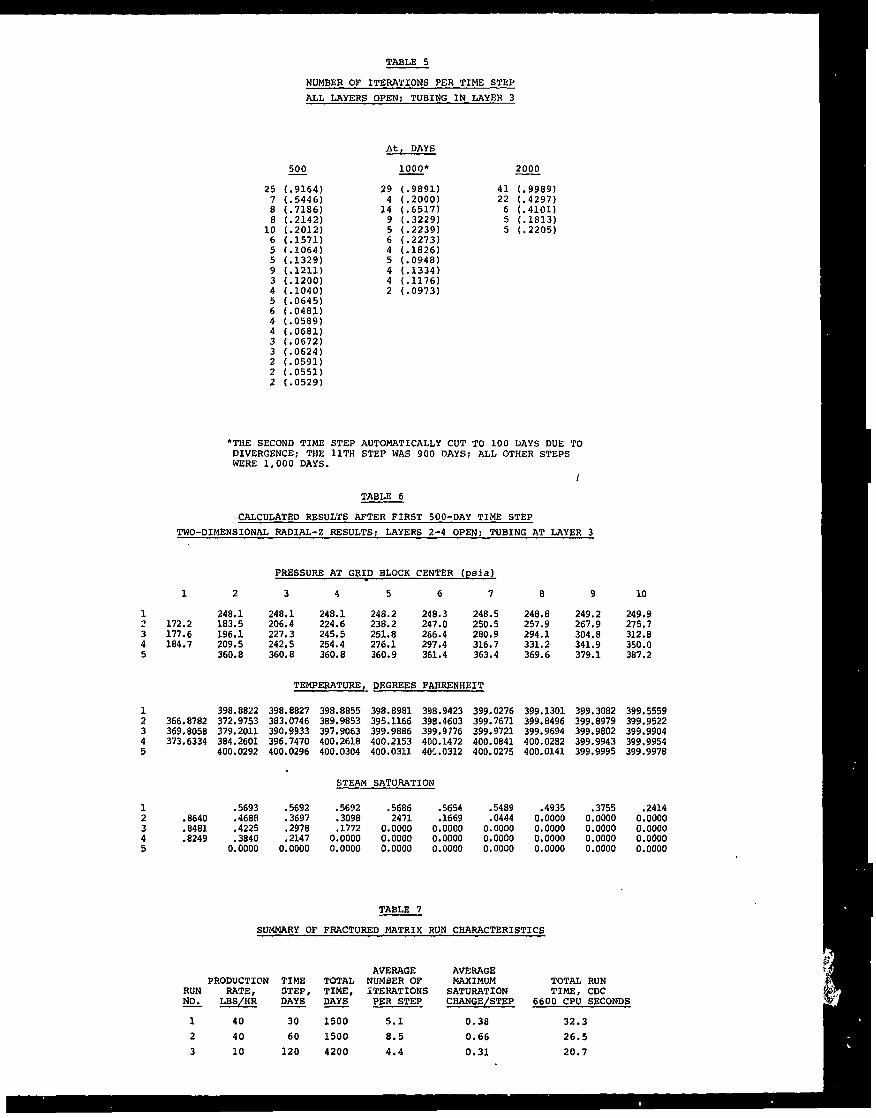
TABLE 5

NUMBER OF ITERATIONS PER TIME STEP

ALL LAYERS OPEN; TUBING IN LAYER 3

500—

25 (.9164)7 (.5446)8 (.7186)8 (.2142)10 (.2012)6 (.1571)5 (.1064)5 (.1329)9 (.1211)3 (.1200)4 (.1040)5 (.0645)6 (.0481)4 (.0589)4 (.0681)3 (.0672)3 (.0624)2 (.0591)2 (.0551)2 (.0529)

*THE SECOND TIME STEPDIVERGENCE; THE 11THW5RE 1,000 DAYS.

At, DAYS

1000*

29 (.9891)4 (.2000)14 (.6517)9 (.3229)5 (.2239)6 (.2273)4 (.1826)5 (.0948)4 (.1334)4 (.1176)2 (.0973)

2000

41 (.9989)22 (.4297)6 (.4101)5 (.1813)5 (,2205)

AUTOMATICALLY CUT TO 100 DAYS DUE TOSTEP WAS 900 DAYS; ALL OTHER STEPS

I

TABLE 6

cmcuLATED RESULTS APTER FIR.9T500-DAY TIME STEP

TWO-DIMENSIONAL RADIAL-Z RESULTS; LAYERS 2-4 OPEN; TUBING AT LAYER 3

PRESSURE AT GRID BLOCK CENTER (psia)

1 2 3 4 5 6 7 8 9 10

248.1 248.1 248.1 248.2 248.3172.2

24S.5 248.8183.5

249.2 249.9206.4 224,6 238.2 247.0 250,5 257.9

177.6267.9

196.1275.7

227.3 245.5 251.8 266.4 280,9184.7

294.1 304.8209.5

312,8242.5 254.4 276.1 297.4 316.7 331.2 341,9

360.8350.0

360.8 360.8 360.9 361.4 363.4 369.6 379,1 387.2

TEMPERATURE, DEGREES FAHRENHEIT

398.8822366.87S2 372.9753369.8058379.2011373.63343S4.2601

400.0292

.5693.8640 .4688.8481 .4225.8249 .3840

0.0000

398.882739S.8855 398.8981398.9423399.02763S3.0746389.9853395.1166398.4603399.7671390.9933397.9063399.9886399.9?76 399.9721396.7470400,261S400.2153400.1472400.0841400.0296400.0304400.031140S.0312400.0275

STEAM SATURATION

.5692 .5692 .5686 .5654 .54s9

.3697 .3098 2471 .1669 .0444

.2978 .1772 0.0000 0.0000

.21470.0000

0.0000 0.0000 0.0000 0.00000.0000 0.0000 0.0000 0.0000 0.0000

399.1301399.8496399.9694400.0282400.0141

.49350.00000.00000.00000.0000

399.3082299.8979399.9802399.9943399.9995

.37550.00000.00000.00000.0000

399.5559339.9522399.9904399,9954399.997s

.24140.OOOO0.00000.00000.0000

TABLE 7

SUMMARY OF FRACTURED MATRIX RUN CHARACTERISTICS

AVERAGE AVERAGEPRODUCTION TIME TOTAL NUM13EROF MAXIMUM TOTAL RUN

RUN ~TE , STEP, TIME, ITERATIONS SATURATION TIME, CDCNO w—.—. DAYSJ DAYS PER STEP CHANGE/STEP 6600 CPU SECONDS

1 40 30 1500 5.1 0.38 32.3

2 40 60 1500 8.5 0.66 26.5

3 10 120 4200 4.4 0.31 20.7

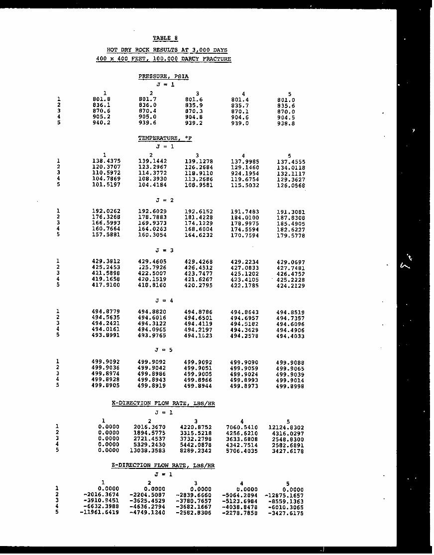
TABLE 8

HOT DRY ROCK RZSULTS Al’3,000 DAYS

400 x 400 FEET, 100,000 DARCY FRACTURE

PRESSURE, PSIAJ=l

1801.8836.1870.6905.2940.2

138?4375120.3707110.5972104.7869101.5197

192.0262176.3268166.5993160.7664157.5881

429.3812425.2453421.5898419.1658417.9100

494.8779494.5635494.2421494.0161493.8991

499.9092499.9036499.8974499.8928499.8905

801f7836.0

801:6835.9

870.4 870.3905.0 904.8939.6 939.2

TEMPERATURE, “F

J=l

2139.1442123.2967114.3772108.3930104.4184

J2=

192.6029178.7883169.9373164.0263160.3054

J3.

429.4605;25.7926422.5007420.1519418.8160

J4=

494.8820494.6016494.3122494.0965493.9765

J=5

499.9092499.9042499.8986499.8943499.8919

3139.1278126.2684118.9110113.2686108.9581

192.6152181.4228174.1229168.6004164.6232

429.4268426.4512423.7477421.6267420.2795

494.8786494.6501494.4119494.2197494.1L23

499.9092499.9051499.9005499.8966499.8944

X-DIRECTION FLOW RATE, LBS/HR

J=l

20:0000 2016.3670 4220?87520.0000 1894.5775 3315.52180.0000 2721.4537 3732.27980.0000 5329.2430 5442.08780.0000 13038.3583 8289.2342

Z-DIRECTIONFLOW RATE, LBS/HR

J=l

10.0000 0:0000 0?0000

-2016.3674 -2204.5087 -2839.6660-3910.9451 -3625.4529 -3780.7657-6632.3988 -4636.2794 -3682.1667-11961.6419 -4749.1240 -2582.8306

801f4835.7870.1904.6939.0

137:9985129.1460924.1954119.6754115.5032

191.7483184.0100178.9975174.5594170.7594

429.2234427.0833425.1202423.4105422.1785

494.8643494.6957494.5182494.3629494.2578

499.9090499.9059499.9024499.8993499.8973

47060.54104256.62103633.68084342.75145706.4035

40.0000

-5064.2894-5123.6984-4038.8478-2278.7858

801!0835.6870.0904.5938.8

5137.4555134.0118132.1117129.3627126.0568

191.3081187.8308185.4905182.6227179.5778

429.0697427.7481426.4752425.2228424.2129

494.8519494.7357494.6096494.4906494.4033

499.9088499.9065499.9039499.9014499.8998

12124:83024316.02972548.83002582.68913427.6178

0?0000-12875.1657-8559.1363-6010.3065-3427.6175

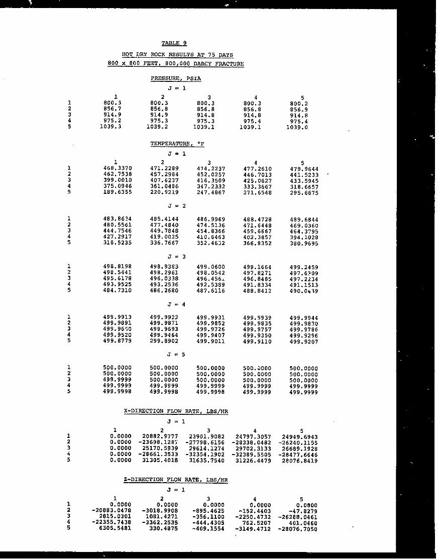
12

:5

12

5

12345

12345

;345

12345

12

5

TABLE 9

HOT rJRY ROCK RESULTS AT 75 DAYS

800 X 800 FEET, 800,000 DARCY F~CTURE

1800.3856.7914.9975.2

1039.3

1468.3370462.7538399.0010375.0946189.6355

483.8624480.5561444.7546427.2917318.5235

498.8198498.5441495.6178493.9525484.7310

499.9913499.9891499.9650499.9520499.8779

500.0000500.0000499.9999499.9999499.9998

PRESSURE, E’SIA

J=l

800:3 800:3856.8 856.8914.9 914.8975.3 975.3

1039.2 1039.1

TEMPERATURE, “F

J=l

471:2289457.2984407.6237361.0486220.9219

J=2

485.4144477.4840449.7848419.0025336.7667

J3.

498.9383498.2961496.0338493.2536486.2680

J=4

499.9922499.9871499.9693499.9464299.8902

J=5

500.0000500.0000500.0000499.9999499.9998

474:2237452.0257416.3509347.2332247.4867

486.9969474.5:36454.8366410.6463352.4632

499.0600498.0542496.456L492.5389487.6116

499.9931499.9852499.9726499.9407499.9011

500.0000500.0000500.0000499.9999499.9998

X-DIRECTION FLOW RATE, LBS/HR

J1=

800:3856.8914.8975.4

1039.1

477:2610446.7013425.0627333.3667271.6548

488.4728471.6448459.6667402.3857366.8352

499.1664497.8271496.8485491.8334488.8412

499.9939499.9835499.9757499.9350499.9110

5oo.aooo500.0000500.0000499.9999499.9999

1 40.0000 20882:9777 23901:9082 24797.30570.0000 -23698.1287 -27798.6156 -28338.04820.0000 25170.5939 29614.1274 29702:31330.0000 -28661.3533 -32354.1902 -32389.55050.0000 31305.4018 31635.7540 31226.4479

Z-DIRECTION FLOW RATE, LBS/HR

J1=

10.0000 0:0000 0?0000 0!0000

-20883.0478 -3018.9908 -895.4625 -152.44032815.0301 1081.4271 -356.1100 -2250.4732

-22355.7438 -3362.2535 -444.4305 762.52076305.5481 330.4875 -409.1554 -3149.4712

5800.2856.9914.8975.4

1039.0

5479.9644441.5233 ‘433.5945318.6657295.6675

489.6844469.0360464.3795394.1028380.9695

499.2459497.6309497.2234491.1513490.0439

499.9944499.9820499.9786499.9296499.9207

500.0000500.0000500.0000499.9999499.9999

24949;6943-26240.115526689.1928

-28477.664628076.8419

0:0000-47.8279

-26288.0461401.0460

-28076.7050

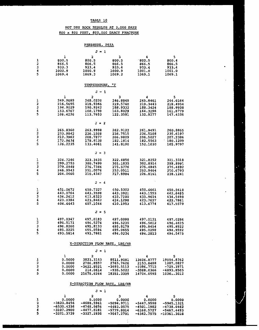
123

;

12345

123~5

12345

12345

12345

TABLE 10

HOT DRY ROCK RESULTS AT 3,000 DAYS

800 X 800 FEET, 800,000 DARCY FRACTURE

1800.5866.5933.31000.91069.4

249:9689216.5695194.9029153.6767106.4226

265.8360233.9842212.3962172.9634126.2235

324.7246299.2753279.0948246.9943204.0660

451.0672443.0764434.2412423.0384404.4443

497.0347496.5171496.8260495.0225493.5814

PRESSURE, PSIA

J=l

3800?5 800.5866.5 866.5933.4 933.41000.9 1000.91069.3 1069.2

TEMPERATURE,‘F

J1=

248:0220218.9366190.9242160.1790113.7653

J2=

263.9998236.1508208.7877178.9138133.4061

J=3

323.3435300.7499276.7346251.0076210.4347

J=4

450.7327443.3598433.8323423.8462407.1044

J=5

497.0183496.5274495.8133495.0594493.7861

246?8849219.5740188.9332163.8029122.3591

262.9122236.7515206.9809182.1814141.8190

322.4850301.1835275.5776253.0511217.8984

450.5302443.3921433.7200424.1298410.1953

497.0098496.5235495.8179495.0655494.0234

X-DIRECTION FLOW RATE, LBS/HR

!?=1

1 2 30.0000 3823.3153 8511.90810.0000 2706.8557 2765.76260.0000 -3422.8521 -3693.51120.0000 214.0614 -935.50220.0000 21678.6244 18351.3309

Z-DIRECTION FLOW RATE, LBS/HR

J=l

1 20.0000 0.0000 0:0000

-3823.8456 -4688.5961 -5094.9711-6530.4336 -4748.0656 -4483.0575-3107.2900 -4477.0181 -5779.8014-3321.3739 -3327.2930 -3647.2701

“800:5S66.5933.41001.01069.1

4245.8461219.3443188.3424164.3298132.9277

261.9491236.5108206.5027182.5563152.1030

321.8252300.8914275.4845252.9464226.8161

450.4661443.1553433.9624423.7657413.6774

497.0131496.5012495.8454495.0298494.2813

413606.87772153.8488-2396.7712-3068.036614704.0595

0!0000-5447.9598-4501.1982-6168.5727-4342.7575

800:4866.5933.4 .

1001.01069.1

5244.6164218.4954188.9908161.8779147.4336

260.8865235.6197207.2386180.1299165.9797

321.3318299.899127rj.4692250.6793238.1241

450.5618442.6485

.

434.5498422.7861417.5579

497.0286496.4625495.8922494.9592494.5475

19054:83521207.0827-729.3971

-4893.85051036..3012

0:0000-5945.1321-4738.0462-5467.4493-10361.3018

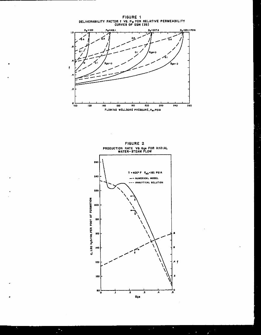
rlwun= I

DELIVERABILITY FACTOR f VS. PW FOR RELATIVE PERMI :ABILITYCURVES OF EON ( 26)

PslA. w --- . . . . . . .1.0 I 1 ~ 1 1 A I I I 1 ~

.8

.6

f

.4

-1oo I 20 140 160 180 200 220 240 260

FLOWING WELLBORE PRESSURE, PW,PSIA

FIGURE 2PRODUCTION RATE VS. Sg8 FOR RADIAL

WATER-STEAM FLOW

2.60

:\T*400° F f’Wb=160PSIA

240

220 .

120

100

60

— NUMERICAL MOOIZL

--- ANALYTICALSOLUTION

\

\

\

\

+

\

\

\

\

0

0 P \0

/ \/

0 \0

\

.s

.6

.4 f

.2

t t I 1

.1 .2 .3 A .6°

. sQe

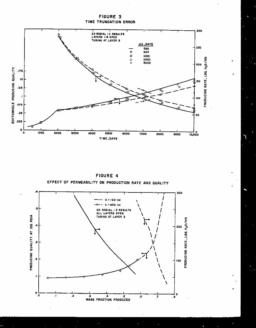
FIGURE 3TIME TRUNCATION ERROR

I I I I I 1 1 1A 20 RADIAL -i RESULTS

\

LAYERS I-5 OPENTUBINO AT LAYER 3

k At *DAYS

\

‘\ — 250

\o 6000 1000~ 2000

\ x 6000

‘h

1=1-g .026

-/ ,0 1 I I to

1 I1000

I2000 3000 4000 6000 6000 7000 8000 Sooo 10

TIME, DAYS

FIGURE 4EFFECT OF PERMEABILITY ON PRODUCTION RATE AND QUALITY

.6 i I I. 1 I I I I I

I

\

— k=100md \“/

+- k = 600 md \ I

\

20 RAOIAL - Z RESULTS \ALL LAYERS OpEN

\/

TUSINL?AT LAYER 3 /

h \\ \.P4

\

\i

v/\‘f/ \

/’ \

0L-.,2 \I I t I

oI

.1 .3 .4 .6MASS FRACTION PRODU%ED

.7D

300

1230

I

Ks

200 2Xw

:-1.

50 ~aa

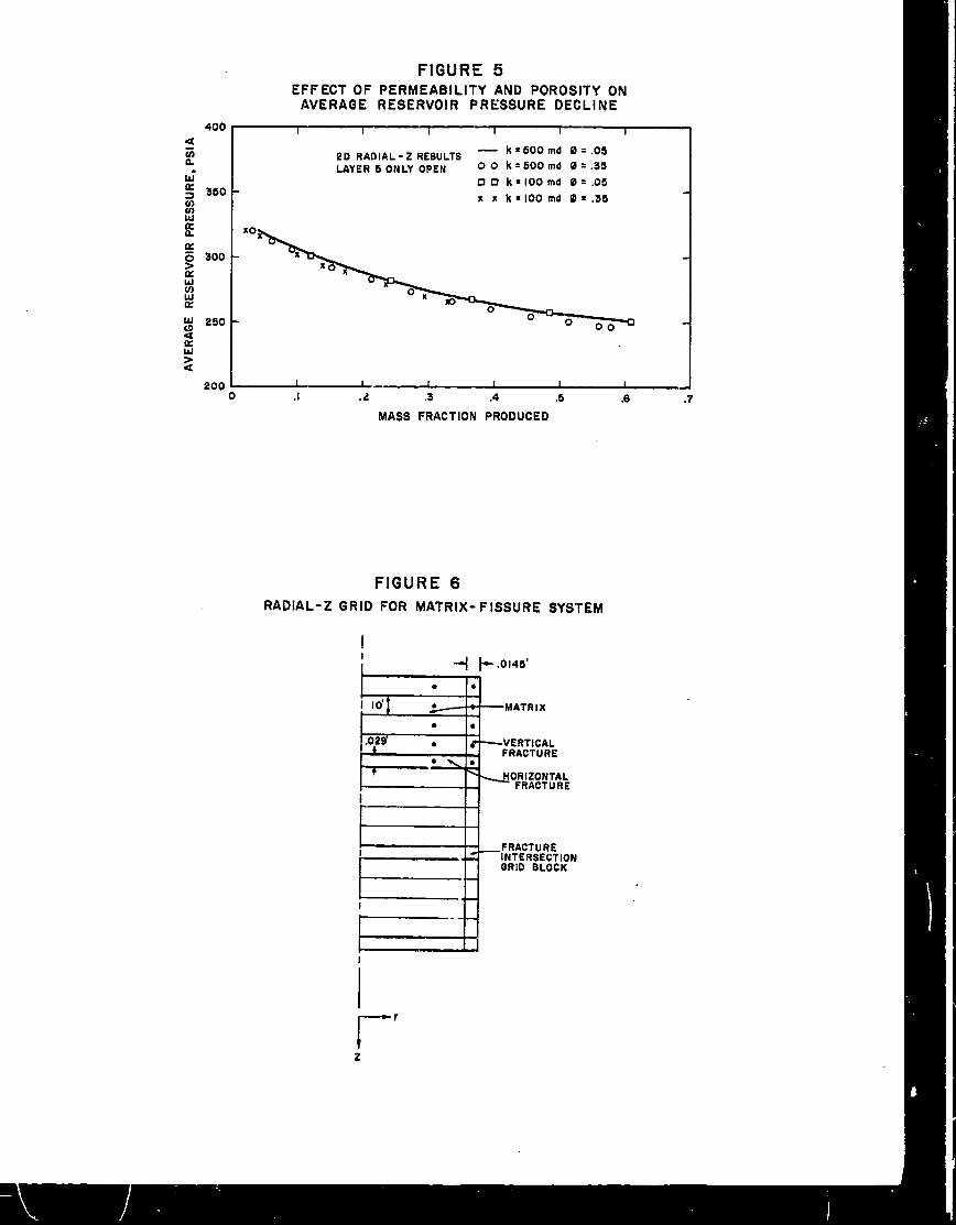
FIGURE 5EFFECT OF PERMEABILITY AND POROSITY ON

AVERAGE RESERVOIR PRIESSURE DECLINE

400 I I I I 1 I<G 2D RADIAL -Z RESULTS

— k=600md 0=.05n

LAYER 50NLY OPEN 00 k=500md Q= .35w“

g 350 -OOk=l OOmd 0=.05

co xxk=lOOmd O= .35

nIXL %0

KG 300> x

%

2K ou 250 00

0

e00

R>a

200 ~~o ,1 .2 .3 .4 ,5 .6 .7

MASS FRACTION PRODUCED

FIGURE 6RADIAL-Z GRID FOR MATRIX- FISSURE SYSTEM

II

1

E● ●

I 10’ ●

● 9

.029 . J

● ●

.0145’

-MATRIX

-VERTICALFRACTURE

~ORIZONTALFRACTURE

1r I

II

1- r

tz

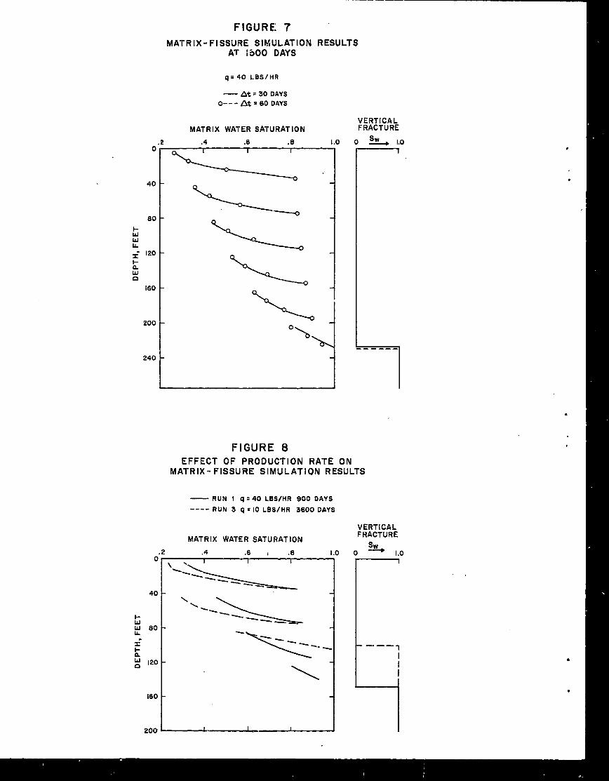
o

40

80

LI&lL=- 120+

:0

160

200

240

0

40

Ltd 80L

s“*ng 120

160

200

iiT :500 DAYS

q=40 LBSIHR

— At= 30 OAYS

o ---& =60 DAYS

MATRIX WATER SATURATION

.2 .4 .6 .8 I .0

%, I

7

.

FIGURE: 7

MATRIX-FISSURE SIMULATION RESULTS

VERTICALFRACTURE

1 ,

.

.

.

VERTICALFRACTURE

SWo - 1.0

I

-.—— 1

:.

I

●

-----

EFFECT OF PRODUCTION RATE ONMATRIX-FISSURE SIMULATION RESULTS

— RUN 1 q = 40 LBS/HR 900 DAYS

---- RUN 3 q =10 LBS/HR 3600 DAYS

MATRIX WATER SATURAT ION

.2 .4 .6 , .8

“’===L.l“’’===-

‘k--\

.*

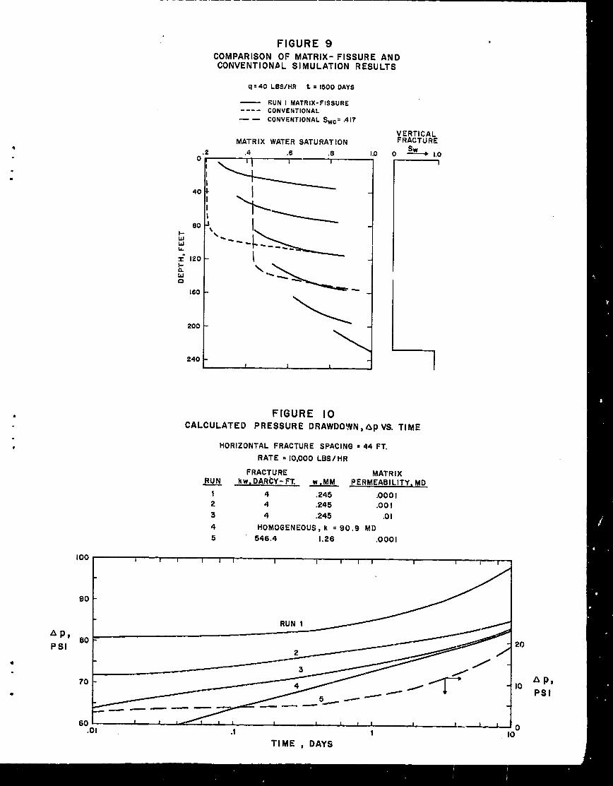
90

APsPsl

80

70

60

a

4C

80

suL

z“ 120

kUo

160

200

240

FIGURE 9 ,

COMPARISON OF MATRIX- FISSURE ANDCONVENTIONAL SIMULATION RESULTS

L

q =40 LBS/HR t = 1500 DAY6

— RUN I MATRIX-FISSURE---- CONVEtiTIONAL— — CONVENTIONAL Swc= .417

MATRIX WATER SATURATION

.4 .6 .8 1.0

‘----i\

“=--\

VERTICALFRACTURE

CALCULATED PRESSURE DRAWDO!VN, Afi) VS. TIME

HORIZONTAL FRACTURE SPACING = 44 FT.

RATE = 10,000 LBS/ HR

FRACTURE MATRIX~ k w. DARCY- FT w,MM PERMEABILITY, MD

1 4 .245 .000 I2 4 .245 .00 I

3 4 .245 .0 I

4 HOMOGENEOUS, k = 90.9 MD

5 546.4 1.26 .0001

100 [ 1 1 I I I I I I I I I I 1 I I I

RUN 1

——— —.—

[ I 1 I I 1 I I 1 1 I 1-. t .J_A_ln

Ap,

Psl

.01 .1 1 10”TIME , DAYS

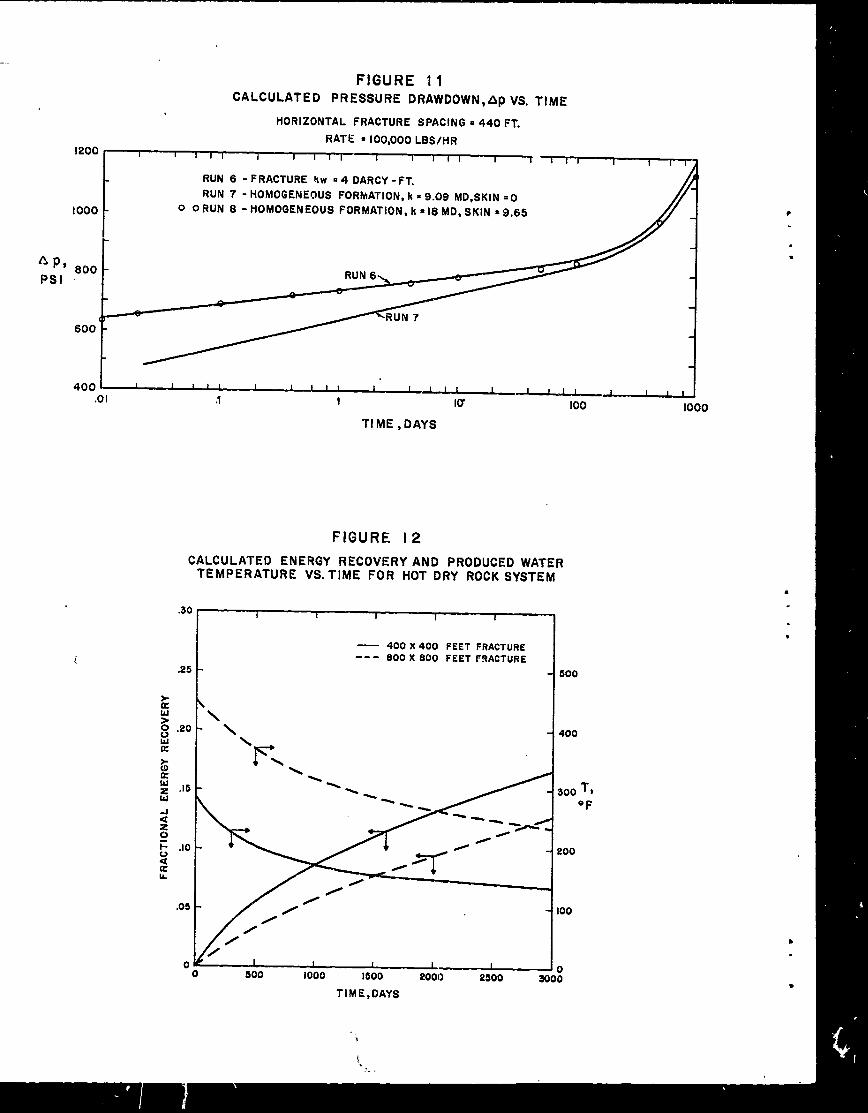
FIGURE 11CALCULATEC) PRESSURE DRAWDOWN, Ap VS. TIME

&p,

Psl

HORIZONTAL FRACTURE SPACING =440 FT.

RATE =loo,ooo LBs/HR

IRUN 6 -FRACTURE #W =4 DARCY -FT.

RUN 7 - HOMOGENEOUS FORMATION, k = 9.09 MD,SKIN =0

1000 - 0 0 RUN 8 - HOMOGENEOUS FORMATION, k s 18 MD, SKIN = 9.65

800 -

600 -

400 t I 1 t 1 I 1

.01~_l_l_u_ 1

.1I I 1

KY 100 1000

TIME , DAYS

FIGURE 12

CALCULATED ENERGY RECOVERY AND PRODUCED WATERTEMPERATURE VS. TIME FOR HOT DRY ROCK SYSTEM

1 — 400 X 400 FEET FRACTURE--- 800 X 800 FEET F!?ACTURE

.25

.

.

..

so”

400

300 T$

‘F

too

00

b

.

TIM E,DAYs

1

!

‘ I.