Embed Size (px)
Citation preview

RMIT University
Econometric Modelling and the Effectiveness of Hedging
Exposure to Foreign Exchange Risk
This paper aims to test the efficiencies of four econometric models at determining an optimal hedge ratio. We will specifically be demonstrating the abilities of each model to outperform each other. The econometric models that we will test include: the (i) Conventional Model (levels), the (ii) Conventional Model (first difference), the (iii) Quadratic Model, and the (iv) Error Correction Model. These four models will be applied to both a money market hedge and a cross currency hedge using the base currency of the Australian Dollar (AUD), an exposure currency of the Canadian Dollar (CAD), and a third currency of the Swiss Franc (CHF). The results will show, that though there is merit in financial hedging; the effectiveness of the hedge is not dependent upon the econometric model chosen.

ii
Disclaimer: All remaining errors and omissions are entirely those of the author.
iii
Table of Contents
1. INTRODUCTION ....................................................................................................................... 1
1. LITERATURE REVIEW ............................................................................................................. 2
1.1 Hedging Techniques ............................................................................................................ 2
1.2 Hedge Ratios ......................................................................................................................... 3
1.3 Econometric Techniques ...................................................................................................... 3
1.4 Measure of Effectiveness and Variance Ratio (VR)/ Variance Reduction (VD) ............. 5
3. METHODOLOGY ....................................................................................................................... 5
3.1 Identification of Currencies and Variable .................................................................................. 6
3.2 Estimating the Money Market Hedge Ratio ............................................................................. 6
3.2.1 Conventional Model (Levels) ............................................................................................... 6
3.2.2 Conventional Model (First Differences).............................................................................. 6
3.2.3 Quadratic Model ................................................................................................................... 6
3.2.4 Error Correction Model ........................................................................................................ 7
3.3 Estimating the Cross Currency Hedge Ratio ............................................................................ 7
3.3.1 Conventional Model (Levels) ............................................................................................... 7
3.3.2 Conventional Model (First Differences).............................................................................. 7
3.3.3 Quadratic Model ................................................................................................................... 7
3.3.4 Error Correction Model ........................................................................................................ 7
3.4 Estimating VR and VD ......................................................................................................... 7
4. DATA AND EMPIRICAL RESULTS ......................................................................................... 8
4.1 Money Market Hedge Results .................................................................................................... 8
4.2 Cross Currency Hedge Results ................................................................................................... 9
4.3 Data and Statistical Outputs ..................................................................................................... 10
5. CONCLUSION ........................................................................................................................... 12
REFERENCES ................................................................................................................................... 14
APPENDICES .................................................................................................................................... 16
Appendix 1: EViews for Money Market Hedge ............................................................................ 16
Appendix 2: EViews Output for Cross Currency Hedge .............................................................. 17

1
1. INTRODUCTION
The objective of this project is to find out if the econometric modelling of the hedge ratio makes
any difference for the effectiveness of money market and cross currency hedging of exposure to
foreign exchange risk.
A major question in finance is the effectiveness of the econometric models being used. It seems
financial types of many kinds put blind faith in the outputs of econometric models, but is this
faith justified? The amount of risk a portfolio manager or CFO is willing to take on is more
often than not based on these models. With the sheer amount of money being wagered by these
money managers, it is essential that these models represent what they promise to.
It was Meese & Rogoff (1983) who showed us that the random walk model often perform better
than any forecast will, but still econometricians believe in their models. In finance and
particularly in the academics it is believed without second thought that a normal distribution is
present, and that the variables follow a random walk. That is to say they are completely random,
and therefore quite impossible to forecast. Still, these econometric models promise to do exactly
this. An entire position and its hedge may very well be based on an econometric model.
The fact that Mark & Choi (1997)and Chinn & Meese (1995) refuted the fact, especially when
forecasts where on a long horizon; provides econometricians with the belief that they can
improve upon the random walk model.
The objective of this study is to test the efficiency of the econometric models when compared
with one another. We will test the (i) Conventional Model (Levels), (ii) Conventional Model
(First Difference), (iii) Quadratic Model, and (iv) Error Correction Model. These models will use
variables derived from the exchange rates between the Canadian Dollar, the Australian Dollar,
and the Swiss Franc. This work is original as the question of effectiveness of hedge ratio
effectiveness based on econometric model has never been approached with these currencies. It
would be recommended that a continuation of the empirical work is undertaken to develop
conclusive answers.
The findings in this study are that none of the econometric models perform better than another.
It is apparent that hedging and using a hedge ratio is advisable, but selection between which
econometric models to use is too little benefit.
This journal will read in the following manner in chapter 1, the introduction, I will introduce the
topic and brief the reader. In chapter 2, I will conduct a literature review and offer an in depth
look into the research available on the topic. Chapter 3 is a discussion on the methodology of the

2
paper and in chapter 4 I will discuss these findings. My conclusions and findings will be
summarised in chapter 5.
1. LITERATURE REVIEW
There are countless studies on the topics discussed, therefore they have been broken up into
distinct sections. This way we can focus on the importance of each to this study, and in the end
see how they are all related. The sections will be as follows: Hedging Techniques, Hedge Ratios,
Econometric Techniques, and measures of effectiveness; specifically Variance Ratio and
Variance Reduction.
1.1 Hedging Techniques
Financial hedging is an important tool in any money management position or position in which
one is taking on risk. There are two types of hedging; both operational and financial.
Operational hedging deals with reducing any exposure to foreign exchange risks, while financial
hedging is the act of taking an opposite position in a holding, to offset the risk that the holdings
move in an unexpected direction. Carter, Pantzalis & Simkins (2003) found that the combined
use of operational and financial hedges is associated with decreased exchange rate exposure. But
the two are complementary of each other, rather than dependent on each other. With operational
hedging having more of a long term focus and financial the short term (Kim, Mathur & Nam
2006). In this study we will be focusing on financial hedging techniques. Yao & Wu (2012),
explain that through financial hedging we can ultimately avoid and resolve the systemic risks that
the position of the original holdings undergo.
In this paper we will be focusing on two types of financial hedging: the money market hedge and
the cross-currency hedge.
In our study the three currencies (AUD, CAD, CHF) were assigned to x, y, and z. These
represented the base currency, exposed currency, and the currency in which would we would
attempt to create a cross rate hedge. Therefore an unhedged position would simply be the
exchange rate between the two, or (x/y). By remaining unhedged any fluctuation in this exchange
rate puts the holder at risk. We also used the interest rates from both our x and y currency, let ix
and iy represent these.
The money market hedge aims to achieve a synthetic forward situation, where the contract rate
would be equal to the interest parity rate (Benet 1992). By borrowing in our base currency and
lending in another we can achieve a money market hedge.

3
To do a cross currency hedge one must take a position on another currency whose exchange rate
against the base currency is correlated with the exchange rate between the base currency and the
exposure currency (Moosa 2011). This is represented by (x/z). Typically these hedges will
involve some form of a futures contract as a hedging tool. Therefore when the spot position and
the futures contract are in the same asset, we can theoretically eliminate a lot of the risk. When
the futures contract and the spot position are in the same asset a high proportion of the risk of
the spot position can be eliminated.
1.2 Hedge Ratios
When trying to create an effective hedge it is common practice that one develops a hedge ratio
(HR). This hedge ratio explains how much of the offsetting position it will require to effectively
hedge the original position. A naïve model assumes that a hedge ratio is equal to one, and it is
considered best practice to start with this assumption. When a hedge ratio is equal to one, the
entire position is hedged. As opposed to either the random walk model or implied model; we use
the naïve model, or a hedge ratio of one (Moosa 2011).
The estimation of the HR is crucial for a successful hedge, but the methods to do so are not
agreed upon. The HR can be explained as the ratio between the total value of one holding
versus’ the total value of the opposite positon (Yao & Wu 2012). Therefore it is essential that
the optimal hedge ratio is estimated, otherwise the risk may not be reduced by the hedge.
Without an optimal hedge ratio we are liable to be over or under hedged, with the potential for
worse losses than an unhedged position.
We measure the optimal hedge ratio through the slope coefficient of the rate of return on the
unhedged position against the rate of return of the hedging tool. The optimal hedge ratio
estimated by OLS will be identical to the hedge ratio estimated from conditional moments.
1.3 Econometric Techniques
A crucial decision made by traders is at what ratio they hedge their spot position at. This is the
problem of choosing an optimal hedge ratio. When trading commodities it a frequently
recommended solution is to set the hedge ratio equal to the ratio of the covariance between spot
and futures prices to the variance of the futures price (Benninga, Eldor & Zilcha 1984). The
estimation of the optimal hedge ratio has undergone a great deal of study in academia. Using the
ideas drawn from portfolio optimization the modern portfolio hedging theory suggested using
the OLS model and a minimum risk profile. Howard & D’Antonio (1984) presented the optimal
Sharpe hedge ratio under the condition of the maximization of the utility function. Junkus & Lee

4
(1985) empirically analysed four kinds of the hedging strategies in light of the maximizing profits,
eliminating risk, minimizing risk as well as maximizing utility(Yao & Wu 2012).
As financial econometricians strive to create a more sophisticated model to estimate hedge ratio,
we are left to use the tools currently available to us. In our study we used the conventional model
or OLS. Citing Myers & Thompson (1989) and note that the use of conventional OLS
estimation implies the use of unconditional sample moments to estimate the optimal hedge ratio
rather than their conditional alternatives.
The OLS does have its downfalls and these come into the fact it may not consider time varying
distributions, serial correlation, heteroskedasticity and cointegration (Poterba & Summers 1987).
We also used the conventional first difference model, also called the simple model and the
historical model. This model amounts to estimating the hedge ratio from historical data by
employing a linear OLS regression at the first difference. When doing this the h is the hedge
ratio and the R2 of the regression measures its effectiveness. Therefore the coefficient is
measuring the speed that deviations from long run values are effectively eliminated. Lien (2004)
argues that the estimation of the hedge ratio and hedging effectiveness may change significantly
when the possibility of cointegration between prices is ignored.
Error correction models have also been suggested, nonlinearity in this case is achieved by
including a polynomial in the error term. Hendry & Ericsson (1991) estimated that a polynomial
to the third degree would be adequate in capturing this adjustment process. The main purpose of
error-correction models is to capture the time series properties of variables, through the complex
lag structures allowed, whilst at the same time incorporating an economic theory of the
equilibrium type (Granger & Weiss 1983). (Lien 2004) provides a theoretical analysis of this
proposition, and ends by saying that a hedger who neglects the cointegrating relationship will not
be taking a big enough offsetting position in the hedge. The empirical results that are resultant of
an error correction model are typically not significantly different from those using either a first
difference or levels model (Moosa 2003).
However, this method has suffered various criticisms. It was shown by Poterba and Summers
(1986) that stocks returns typically exhibit time-varying conditional heteroskedasticity and
because of this the assumption that covariance matrix remains constant. To improve upon past
hedge ratio estimations it may worth considering time variance of second moments (Casillo
2004). It is for this reason that recent studies have suggested attempting to use the GARCH
method for hedge ratio estimation (Hatemi-J & Roca 2006). The GARCH method allows the
conditional variances and covariances used as inputs to the hedge ratio to be time-varying.

5
Though there are more complex and time consuming methods, many authors have mentioned
that the more advanced techniques have the potential to exhibit a better performance, they do
not come without some downfalls. Some of these methods can be very problematic to estimate
and can potentially create even more costs (Lien 2004). When it comes down to it, the simple
methods like OLS can achieve results that are just as good (Myers & Thompson 1989).
1.4 Measure of Effectiveness and Variance Ratio (VR)/ Variance Reduction (VD)
When we have a perfect correlation between the prices of the hedged exchange rate and that of
the hedging instrument we achieve a hedge ratio of 1. Therefore a lot of the hedging
effectiveness is related to the correlation between the prices.
The effectiveness of the hedge ratios to foreign exchange risk can be measured by using the
variance ratio (VR) and variance reduction (VD) measures. By testing the equality of the variance
of the rates of return on both the hedged and unhedged position we can measure the VR and
VD (Moosa 2011).
The variance ratio test can be conducted to compare the effectiveness of two hedging positions
resulting from the use of different hedge ratios or different hedging instruments. If the prices of
the two currencies are not perfectly correlated than we should see that the hedge ratio will not be
equal to one. Because of this we can measure the effectiveness of the hedge by the correlation
we see between the prices. Therefore the smaller the variance the more effective the hedge is. It
must also be put through a formal test and the equality between the two must be put to a test.
The effectiveness of the hedge is therefore measured by the variance of the rate of return on the
hedged position compared with the variance of the rate of return on the unhedged position. As
the variance got smaller we would know that the hedge is becoming more effective. The VD on
the helps explain the reduction in variance when using a hedge.
Another method when using any of the models is the coefficient of determination or R2 to help
to determine the effectiveness. If the R2 was equal to one, then we could hope for a perfect
hedge. This could only happen if the prices were deemed to be perfectly correlated; in either a
positive or negative direction. Therefore if the coefficient of determination (R2) is equal to one
than we have achieved a perfect hedge.
3. METHODOLOGY
As the methods to measure the predictive accuracy of econometric modelling and their
effectiveness on hedge ratios involve the estimation and testing of the four models using EViews

6
8 and Microsoft Excel 2013, this chapter is best divided into subsections identifying each stage
of testing and or estimation procedure.
In this chapter the “variables‟, which are often referred to, are those which have been derived
from the manipulation of the original data set sourced from Bloomberg. These variables include
the exchange rates of the countries and their respective interest rates.
3.1 Identification of Currencies and Variable
As mentioned before, in our study the three currencies (AUD, CAD, CHF) were assigned to x, y,
and z. Each currency represented the base currency, exposed currency, and the currency in
which would we would attempt to create a cross rate hedge. The exchange rate between the two
(AUD/CAD) is represented by x/y. By remaining unhedged any fluctuation in this exchange rate
puts the holder at risk. Other variables used included the interest rates of Australia and Canada;
represented as ix and iy respectively.
3.2 Estimating the Money Market Hedge Ratio
To estimate the money market hedge ratio between x and y we used the following formula:
y
x
i
iyxSyxF
1
1)/(),( [1]
This estimation is representative of the interest parity forward rate between the two.
3.2.1 Conventional Model (Levels)
The conventional model used the following formula:
ttt fhs [2]
In equation 2 the variables are equal to fyxF ))/(log( and syxS ))/(log( .
3.2.2 Conventional Model (First Differences)
The first difference estimates with a lag of one, the formula is as follows:
ttt fhs [3]
3.2.3 Quadratic Model
The Quadratic Model equation is equal to:
tttt ffhs 2 [4]

7
3.2.4 Error Correction Model
The Error Correction Model (ECM) is as follows:
tttttt ffhss 111 [5]
3.3 Estimating the Cross Currency Hedge Ratio
Again in the cross currency hedge ratio we will use an unhedged position and a hedging tool which
will be equal to (x/y) and function of (x/z) where 1))/(log( syxS and 2))/(log( szxS ,
respectively. We will use the following models once again to estimate the hedge ratios.
3.3.1 Conventional Model (Levels)
The conventional model uses the following formula:
ttt hss 21 [6]
3.3.2 Conventional Model (First Differences)
The first differences model uses the following formula:
ttt shs 21 [7]
3.3.3 Quadratic Model
The quadratic model used the following formula:
tttt shss 2
221 [8]
3.3.4 Error Correction Model
The ECM used the following formula:
tttttt sshss 11,221,11 [9]
3.4 Estimating VR and VD
Calculating the VR and VD for the estimated hedge ratios is the next step, and our attempt to
measure the estimations successes. The variance ratio is equal to the ratio of the variance of the
return of the unhedged position to the variance of the rate of return on hedged position. To
calculate VR we will use one of the following equations:
)(
)(2
2
fhs
sVR
[10]
Or:

8
)(
)(
21
2
1
2
shs
sVR
[11]
In this calculation )()( 1
22 ss is equal to the variance of the rate of return on the
unhedged positon and ( )(2 fhs or )( 21
2 shs ) is equal to the variance of the rate of
return on the hedged position. When calculating VR, we can then decide if it is and effective
hedge by using this equation:
)1,1( nnFVR [12]
VD is simply calculated as:
VRVD
11 [13]
4. DATA AND EMPIRICAL RESULTS
In this study we estimated the hedge ratio from four different econometric models across two
different hedging techniques. The intention of the study was to discover whether the model used
makes any difference for the effectiveness of the hedge. The objective is to find out whether the
estimation method or model specification makes any difference for hedging effectiveness. The
two hedging techniques used will be the money market hedging and cross currency hedging.
Many studies have attempted a similar study, but with different econometric models such as
(Longo et al. 2007).
Figure 1 plots the rates of return for the unhedged position against the hedged positions for the
money market hedge. In Figure 2 we can see the results of the unhedged position versus that of
the hedged position in the cross currency hedge. Table 1 shows the estimations results from the
EViews outputs. From these outputs we can see the hedge ratio, the t-statistic, and the R2 or
coefficient of determination. In Table 2 are the variance ratio and variance reduction as well as
the variance of the unhedged position.
4.1 Money Market Hedge Results
Figure 1 looks at the rates of return of the unhedged versus the hedged rates of return; against
each econometric model for the purpose of a money market hedge. As we can see, regardless of
which method is used we see a success with the hedge. As the variance of the hedge approaches
zero, we are getting closer to a perfect hedge. In Table 2, we also see the variance ratio is
statistically significant in every case.

9
Figure 1: Variance of Rates of Return on the Unhedged and Hedged Positions (Money
Market Hedging)
Levels First Difference
Quadratic Error Correction
4.2 Cross Currency Hedge Results
We now assess the success of the cross currency hedge. Though the variance is much higher
than what we saw with the money market hedge, we still achieved a lower variance ratio than the
unhedged position achieved. But between econometric models the success was consistent
between them. Consider now cross currency hedging. The difference between the results
achieved under money market hedging and cross currency hedging is correlation (Moosa 2011).
-8
-6
-4
-2
0
2
4
6
8
10
12
Unhedged Vs. First Difference
Unhedged Conventional (First)
-10
-5
0
5
10
15
Unhedged Vs. Conventional
Unhedged Coventional
-8
-6
-4
-2
0
2
4
6
8
10
12
Unhedged Vs.Quadratic
Unhedged Quadratic
-8
-6
-4
-2
0
2
4
6
8
10
12
Unhedged Vs. ECM
Unhedged ECM

10
Figure 2: Variance of Rates of Return on the Unhedged and Hedged Positions (Cross
Currency Hedging)
Levels First Difference
Quadratic Error Correction
4.3 Data and Statistical Outputs
When analysing Table 1 and Table 2, a few things become apparent. Each econometric model
was successful at improving on the variance of an unhedged position. But they were all
successful to virtually the same degree of success. More testing could be done to see if the small
differences are significant or not. Also all numbers where statistically significant.
-8
-6
-4
-2
0
2
4
6
8
10
12
Unhedged Vs. Conventional
Unhedged Coventional
-8
-6
-4
-2
0
2
4
6
8
10
12
Unhedged Vs. First Difference
Unhedged Conventional (First)
-8
-6
-4
-2
0
2
4
6
8
10
12
Unhedged Vs. Quadratic
Unhedged Quadratic
-8
-6
-4
-2
0
2
4
6
8
10
12
Unhedged Vs. ECM
Unhedged ECM

11
Table 1: The Estimated Hedge Ratios
Hedging Method/Model Estimated h t Statistics 2R
Money Market
Levels
1.003197 746.4471 0.999758
First Differences
1.002283 1438.408 0.999935
Quadratic
.999667 213.0824 0.999759
Error Correction
1.002324 1470.821 0.999759
Cross Currency
Levels
.321832 4.925604 0.152338
First Differences
.313633 5.196754 0.167734
Quadratic
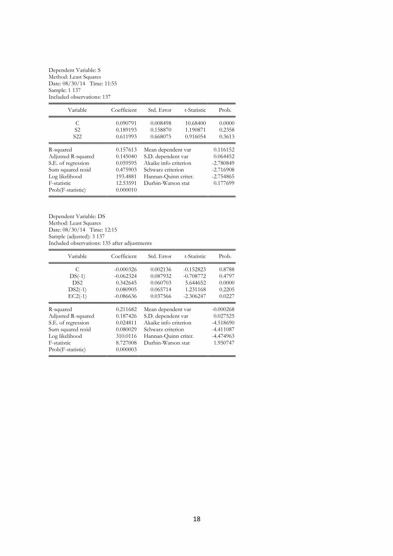
.189193 1.190871 0.157613
Error Correction
.342645 5.644652 0.211682

12
Table 2: Report the estimated VD and VR as in Table 2.
Hedging Method/Model Variance
(Unhedged)
Variance
(Hedged)
VR VD
Money Market
Levels
7.547234806 0.000498175 15217.71525 0.999934287
First Differences
7.547234806 0.000490837 15445.22682 0.999935255
Quadratic
7.547234806 0.000539529 14051.31754 0.999928832
Error Correction
7.547234806 0.000490896 15443.36927 0.999935247
Cross Currency
Levels
13.19446762 6.306547179 1.20209876 0.168121594
First Differences
13.19446762 6.305088259 1.202376911 0.168314036
Quadratic
13.19446762 6.50072812 1.166191295 0.142507748
Error Correction
13.19446762 6.318217792 1.199878319 0.166582157
5. CONCLUSION
The objective of this study was to measure the effectiveness of econometric models to estimate
the hedge ratio. And more specifically is one model better than the next. We tested the
Conventional Model, the Conventional Model with first differences, the Quadratic model, and
the Error Correction Model.
Though econometric models are a popular tool in finance, this paper shows that they might not
hold as much power as financial minds like to think. The four models tested to estimate a hedge
ratio are essentially useless when compared against one another. The amount of time spent
researching and developing these models may have been for naught.
With the money market hedge the study was able to create an almost perfect hedge. This is
possible because of a high correlation between the spot and interest parity rates. Because the
currencies for the cross currency hedge are not as highly correlated we do not achieve as
effective of a hedge. Because of this, a hedge ratio of one produces a cross currency hedge that is
less effective than with the money market hedge. That is why by using the correlation coefficient
between the two spot rates, we are able to create an effective hedge.

13
Based on this study, we can be confident that a hedging technique will help you minimize the
variance of the rate of returns, but the econometric model chosen to derive this does not matter.
It was Moosa (2003) who said it best, “Although the theoretical arguments for why model
specification does matter are elegant…what really matters for the success or failure of a hedge is
the correlation between the prices of the unhedged position and the hedging instrument”. And
this issue in correlation is why we see the difference with the money market hedge and the cross
currency.
Some considerations need to be made. As a follow up to this study a test of more econometric
models would be recommended. ARCH, GARCH, and ARIMA models may be considered and
tested. Though Casillo (2004) found that a multivariate GARCH model is only ‘marginally better’
than other. These marginal differences would need to be tested for significance. Moosa (2003)
found similar results to Casillo. However, in a study by Byström (2003) in a study of the hedging
effectiveness of the electricity futures contracts in Norway from January 1996 to October 1999,
he found that the OLS performed slightly better. It is because of this that I recommend the
GARCH method be attempted, but would not expect drastically different results.

14
REFERENCES
Benet, BA 1992, ‘Hedge period length and Ex-ante futures hedging effectiveness: The case of foreign-exchange risk cross hedges’, Journal of Futures Markets, vol. 12, no. 2, pp. 163–175.
Benninga, S, Eldor, R & Zilcha, I 1984, ‘The optimal hedge ratio in unbiased futures markets’, Journal of futures markets, vol. 4, no. 2, pp. 155–159.
Byström, HN 2003, ‘The hedging performance of electricity futures on the Nordic power exchange’, Applied Economics, vol. 35, no. 1, pp. 1–11.
Carter, D, Pantzalis, C & Simkins, B 2003, ‘Asymmetric exposure to foreign exchange risk: financial and real option hedges implemented by US multinational corporations’, in Proceedings from the 7th Annual International Conference on Real Options: Theory Meets Practice. Washington, DC, accessed October 13, 2014, from <http://realoptions.org/papers2003/SimkinsMNC_Paper.pdf>.
Casillo, A ‘Model Specification for the Estimation of the Optimal Hedge Ratio with Stock Index Futures: an Application to the Italian Derivatives Market’, accessed October 7, 2014, from <http://jamesgoulding.com/Research_II/Hedging%20Concepts/Hedging%20(Equity%20Index%201).pdf>.
Chinn, MD & Meese, RA 1995, ‘Banking on currency forecasts: How predictable is change in money?’, Journal of International Economics, vol. 38, no. 1, pp. 161–178.
Granger, CW & Weiss, AA 1983, ‘Time series analysis of error-correction models’, Studies in Econometrics, Time Series, and Multivariate Statistics, pp. 255–278.
Hatemi-J, A & Roca, E 2006, ‘Calculating the optimal hedge ratio: constant, time varying and the Kalman Filter approach’, Applied Economics Letters, vol. 13, no. 5, pp. 293–299.
Hendry, DF & Ericsson, NR 1991, ‘Modeling the demand for narrow money in the United Kingdom and the United States’, European Economic Review, vol. 35, no. 4, pp. 833–881.
Howard, CT & D’Antonio, LJ 1984, ‘A risk-return measure of hedging effectiveness’, Journal of Financial and Quantitative Analysis, vol. 19, no. 01, pp. 101–112.
Junkus, JC & Lee, CF 1985, ‘Use of three stock index futures in hedging decisions’, Journal of Futures Markets, vol. 5, no. 2, pp. 201–222.
Kim, YS, Mathur, I & Nam, J 2006, ‘Is operational hedging a substitute for or a complement to financial hedging?’, Journal of Corporate Finance, vol. 12, no. 4, pp. 834–853.
Lien, D 2004, ‘Cointegration and the optimal hedge ratio: the general case’, The Quarterly Review of Economics and Finance, vol. 44, no. 5, pp. 654–658.
Longo, C, Manera, M, Markandya, A & Scarpa, E 2007, ‘Evaluating the empirical performance of alternative econometric models for oil price forecasting’, accessed October 14, 2014, from <http://works.bepress.com/matteo_manera/2/>.

15
Mark, NC & Choi, D-Y 1997, ‘Real exchange-rate prediction over long horizons’, Journal of International Economics, vol. 43, no. 1, pp. 29–60.
Meese, RA & Rogoff, K 1983, ‘Empirical exchange rate models of the seventies: Do they fit out of sample?’, Journal of international economics, vol. 14, no. 1, pp. 3–24.
Moosa, I 2003, ‘The sensitivity of the optimal hedge ratio to model specification’, Finance Letters, vol. 1, no. 1, pp. 15–20.
Moosa, IA 2011, ‘The Failure of Financial Econometrics: Estimation of the Hedge Ratio as an Illustration’, The Capco Institute Journal of Financial Transformation, vol. 31, pp. 67–71.
Myers, RJ & Thompson, SR 1989, ‘Generalized Optimal Hedge Ratio Estimation’, American Journal of Agricultural Economics, vol. 71, no. 4, pp. 858–868.
Poterba, JM & Summers, LH 1987, The persistence of volatility and stock market fluctuations, National Bureau of Economic Research Cambridge, Mass., USA, accessed October 13, 2014, from <http://www.nber.org/papers/w1462>.
Yao, Z & Wu, H 2012, ‘Financial Engineering Estimation Methods of Minimum Risk Hedge Ratio’, Systems Engineering Procedia, vol. 3, pp. 187–193.

16
APPENDICES
Appendix 1: EViews for Money Market Hedge Dependent Variable: S Method: Least Squares Date: 08/30/14 Time: 11:33 Sample: 1 137 Included observations: 137
Variable Coefficient Std. Error t-Statistic Prob. C -0.001860 0.000180 -10.33411 0.0000
F 1.003197 0.001344 746.4471 0.0000 R-squared 0.999758 Mean dependent var 0.116152
Adjusted R-squared 0.999756 S.D. dependent var 0.064452 S.E. of regression 0.001007 Akaike info criterion -10.94955 Sum squared resid 0.000137 Schwarz criterion -10.90692 Log likelihood 752.0441 Hannan-Quinn criter. -10.93223 F-statistic 557183.3 Durbin-Watson stat 0.048938 Prob(F-statistic) 0.000000
Dependent Variable: DS Method: Least Squares Date: 08/30/14 Time: 11:37 Sample (adjusted): 2 137 Included observations: 136 after adjustments
Variable Coefficient Std. Error t-Statistic Prob. C -1.69E-05 1.90E-05 -0.888554 0.3758
DF 1.002283 0.000697 1438.408 0.0000 R-squared 0.999935 Mean dependent var -0.000290
Adjusted R-squared 0.999935 S.D. dependent var 0.027424 S.E. of regression 0.000222 Akaike info criterion -13.97760 Sum squared resid 6.58E-06 Schwarz criterion -13.93477 Log likelihood 952.4767 Hannan-Quinn criter. -13.96019 F-statistic 2069018. Durbin-Watson stat 2.001766 Prob(F-statistic) 0.000000
Dependent Variable: S Method: Least Squares Date: 08/30/14 Time: 11:38 Sample: 1 137 Included observations: 137
Variable Coefficient Std. Error t-Statistic Prob. C -0.001696 0.000276 -6.145730 0.0000
F 0.999667 0.004691 213.0824 0.0000 F2 0.014002 0.017828 0.785409 0.4336
R-squared 0.999759 Mean dependent var 0.116152
Adjusted R-squared 0.999755 S.D. dependent var 0.064452 S.E. of regression 0.001008 Akaike info criterion -10.93954 Sum squared resid 0.000136 Schwarz criterion -10.87560 Log likelihood 752.3587 Hannan-Quinn criter. -10.91356 F-statistic 277801.3 Durbin-Watson stat 0.051132 Prob(F-statistic) 0.000000

17
Dependent Variable: DS Method: Least Squares Date: 08/30/14 Time: 11:39 Sample (adjusted): 3 137 Included observations: 135 after adjustments
Variable Coefficient Std. Error t-Statistic Prob. C -1.57E-05 1.86E-05 -0.844800 0.3998
DS(-1) 0.008016 0.084707 0.094637 0.9247 DF 1.002324 0.000681 1470.821 0.0000
DF(-1) -0.006047 0.084904 -0.071216 0.9433 EC(-1) -0.027964 0.018697 -1.495684 0.1372
R-squared 0.999941 Mean dependent var -0.000268
Adjusted R-squared 0.999939 S.D. dependent var 0.027525 S.E. of regression 0.000216 Akaike info criterion -14.01080 Sum squared resid 6.04E-06 Schwarz criterion -13.90319 Log likelihood 950.7287 Hannan-Quinn criter. -13.96707 F-statistic 546418.0 Durbin-Watson stat 2.059779 Prob(F-statistic) 0.000000
Appendix 2: EViews Output for Cross Currency Hedge
Dependent Variable: S Method: Least Squares Date: 08/30/14 Time: 11:53 Sample: 1 137 Included observations: 137
Variable Coefficient Std. Error t-Statistic Prob. C 0.087549 0.007721 11.33908 0.0000
S2 0.321832 0.065339 4.925604 0.0000 R-squared 0.152338 Mean dependent var 0.116152
Adjusted R-squared 0.146059 S.D. dependent var 0.064452 S.E. of regression 0.059559 Akaike info criterion -2.789205 Sum squared resid 0.478884 Schwarz criterion -2.746577 Log likelihood 193.0605 Hannan-Quinn criter. -2.771882 F-statistic 24.26157 Durbin-Watson stat 0.176500 Prob(F-statistic) 0.000002
Dependent Variable: DS Method: Least Squares Date: 08/30/14 Time: 12:13 Sample (adjusted): 2 137 Included observations: 136 after adjustments
Variable Coefficient Std. Error t-Statistic Prob. C -0.000313 0.002153 -0.145210 0.8848
DS2 0.313633 0.060352 5.196754 0.0000 R-squared 0.167734 Mean dependent var -0.000290
Adjusted R-squared 0.161523 S.D. dependent var 0.027424 S.E. of regression 0.025111 Akaike info criterion -4.516392 Sum squared resid 0.084498 Schwarz criterion -4.473559 Log likelihood 309.1147 Hannan-Quinn criter. -4.498986 F-statistic 27.00625 Durbin-Watson stat 2.201068 Prob(F-statistic) 0.000001
18
Dependent Variable: S Method: Least Squares Date: 08/30/14 Time: 11:55 Sample: 1 137 Included observations: 137
Variable Coefficient Std. Error t-Statistic Prob. C 0.090791 0.008498 10.68400 0.0000
S2 0.189193 0.158870 1.190871 0.2358 S22 0.611993 0.668075 0.916054 0.3613
R-squared 0.157613 Mean dependent var 0.116152
Adjusted R-squared 0.145040 S.D. dependent var 0.064452 S.E. of regression 0.059595 Akaike info criterion -2.780849 Sum squared resid 0.475903 Schwarz criterion -2.716908 Log likelihood 193.4881 Hannan-Quinn criter. -2.754865 F-statistic 12.53591 Durbin-Watson stat 0.177699 Prob(F-statistic) 0.000010
Dependent Variable: DS Method: Least Squares Date: 08/30/14 Time: 12:15 Sample (adjusted): 3 137 Included observations: 135 after adjustments
Variable Coefficient Std. Error t-Statistic Prob. C -0.000326 0.002136 -0.152823 0.8788
DS(-1) -0.062324 0.087932 -0.708772 0.4797 DS2 0.342645 0.060703 5.644652 0.0000
DS2(-1) 0.080905 0.065714 1.231168 0.2205 EC2(-1) -0.086636 0.037566 -2.306247 0.0227
R-squared 0.211682 Mean dependent var -0.000268
Adjusted R-squared 0.187426 S.D. dependent var 0.027525 S.E. of regression 0.024811 Akaike info criterion -4.518690 Sum squared resid 0.080029 Schwarz criterion -4.411087 Log likelihood 310.0116 Hannan-Quinn criter. -4.474963 F-statistic 8.727008 Durbin-Watson stat 1.950747 Prob(F-statistic) 0.000003


