This file is part of the following reference:

Brown, Lawrence H. III (2012) The energy and

environmental burden of Australian ambulance services.

PhD thesis, James Cook University.

Access to this file is available from:

http://eprints.jcu.edu.au/24343

The author has certified to JCU that they have made a reasonable effort to gain

permission and acknowledge the owner of any third party copyright material

included in this document. If you believe that this is not the case, please contact

ResearchOnline@jcu.edu.au and quote http://eprints.jcu.edu.au/24343

ResearchOnline@JCU

The Energy and Environmental Burden

of Australian Ambulance Services

Thesis submitted by

Lawrence H. Brown III

Master of Public Health and Tropical Medicine

June 2012

For the Degree of Doctor of Philosophy

In the School of Public Health, Tropical Medicine and Rehabilitation Sciences

James Cook University

i

Declarations

Statement of Access

I, the undersigned, author of this work, understand that James Cook University

will make this thesis available for use within the University Library and, via the

Australian Digital Theses network, for use elsewhere.

I understand that, as an unpublished work, a thesis has significant protection

under the Copyright Act. I do not wish to place any further restriction on access to this

work.

______________________________

Lawrence H. Brown III 22 June 2012

ii

Electronic Copy Declaration

I, the undersigned, the author of this work, declare that the electronic copy of

this thesis provided to the James Cook University Library is an accurate copy of the

print thesis submitted, within the limits of the technology available.

______________________________

Lawrence H. Brown III 22 June 2012

iii

Statement of Sources Declaration

I declare that this thesis is my own work and has not been submitted in any form

for another degree or diploma at any university or other institution of tertiary education.

Information derived from the published or unpublished work of others has been

acknowledged in the text and a list of references is given.

______________________________

Lawrence H. Brown III 22 June 2012

(Every reasonable effort has been made to gain permission and acknowledge the owners

of copyright material. I would be pleased to hear from any copyright owner who has

been omitted or incorrectly acknowledged.)

iv

Declaration on Ethics

The research presented and reported in this thesis was conducted within the

guidelines for research ethics outlined in the National Statement on Ethics Conduct in

Research Involving Humans (1999), the Joint NHMRC/AVCC Statement and

Guidelines on Research Practice (1997), the James Cook University Policy on

Experimentation Ethics: Standard Practices and Guidelines (2001), and the James Cook

University Statement and Guidelines on Research Practice (2001).

The research in this thesis received approval from the James Cook University

Human Research Ethics Committee (approval numbers: H3592; H4277; H3982). The

approval documents are included in Appendix 1.

______________________________

Lawrence H. Brown III 22 June 2012

v

Citations for, and the Contributions of Other Authors to, Published or Submitted

Works Resulting from or Contributing to this Thesis

Brown, L.H., Canyon. D.V., Buettner, P.G. (In Press). The energy burden and

environmental impact of health services: A review. American Journal of Public Health.

Based on Chapter 3.

Author contributions: LHB devised and executed the search strategy, reviewed

the identified papers and extracted the relevant data, and drafted the manuscript.

DVC and PGB reviewed and provided guidance on the search strategy, and

provided critical review of the final manuscript.

Brown, L.H., Canyon. D.V., Buettner. P.G., Crawford. J.M., Judd. J., on behalf of the

Australian Ambulance Emissions Study Group. (In Press). The carbon footprint of

Australian ambulance operations. Emergency Medicine Australasia. Based on Chapter

4.

Author contributions: LHB developed the study design and data collection

process, established the linkages with the participating organisations, conducted

the data analysis and drafted the manuscript. DVC, PGB, JMC and JJ provided

comment on the study design, guidance on the interpretation of the findings, and

provided critical review of the final manuscript.

Brown, L.H., Canyon, D.V., Buettner, P.G., Crawford, J.M., Judd, J. (Under Review).

Estimating the complete life cycle emissions of Australian ambulance operations. Based

on Chapter 5.

vi

Author contributions: LHB developed the study design, collected the data,

conducted the data analysis and drafted the manuscript. DVC, PGB, JMC and JJ

provided comment on the study design, guidance on the interpretation of the

findings, and provided critical review of the final manuscript.

Brown, L.H., Chaiechi, T., Buettner, P.G., Canyon, D.V., Crawford, J.M., Judd, J.

(Under Review). How do energy prices impact ambulance services? Evidence from

Australia. Based on Chapter 6.

Author contributions: LHB developed the study design, collected the data,

conducted the primary data analysis and drafted the manuscript. TC provided

guidance on and assisted with the data analysis and the interpretation of the

results. TC, PGB, DVC, JMC and JJ provided comment on the study design,

guidance on the interpretation of the findings, and provided critical review of the

final manuscript.

Brown, L.H., Blanchard, I.E. (2012). Energy, emissions, and emergency medical

services: Policy matters. Energy Policy, 46, 585-593. Portions of the discussion in

Chapter 7 are adapted from this manuscript.

Author contributions: LHB and IEB developed and executed this post hoc

analysis. LHB drafted the manuscript; IEB provided critical review of the

manuscript. A significant revision to the manuscript occurred as a result of the

peer-review process. LHB and IEB contributed equally to that revision.

Documentation of acceptance for manuscripts arising from this thesis that are in press is

included in Appendix 2. The published versions of manuscripts arising from or

vii

contributing to this thesis that were published as of the date of submission are included

in Appendix 3. Contributing author verification of their contributions is included in

Appendix 4.

Contributions by Others to the Thesis as a Whole

Dr. Petra Buettner and Dr. Deon Canyon (my primary supervisors) contributed

significantly to the process of refining and focusing the original concept for this thesis,

and to the drafting of all the Chapters. Dr. John “Mac” Crawford and Dr. Jenni Judd

also provided critical review and comment on the thesis as a whole. Dr. Taha Chaiechi

and Dr. Petra Buettner were both instrumental in my efforts to learn about, and conduct,

the panel data analyses in Chapter 6. Although Ian Blanchard did not formally

contribute to this thesis, he did make substantial contributions to one of the “…Works

Resulting from or Contributing to this Thesis” (as described above) and to the

“Additional Relevant Works … not Forming Part of this Thesis” (described below). I

certainly made use of those shared experiences in completing this work. Also, all of the

Chapters in this thesis that have undergone peer review have benefited greatly from the

feedback of the anonymous reviewers.

Ms. Kim Pritchard provided professional proof reading and editing for this

thesis, limited to Standards D and E of the Australian Standards for Editing Practice.

Parts of the Thesis Submitted to Qualify for the Award of another Degree

None.

viii

Additional Relevant Works Published by the Author but not Forming Part of the

Thesis

Blanchard, I., Brown, L.H. (2009). Carbon footprinting of EMS systems: A proof of

concept study. Prehospital Emergency Care, 13, 546-549.

Blanchard, I.E., Brown, L.H., on behalf of the North American EMS Emissions Study

Group. Carbon footprinting of North American EMS systems. (2011). Prehospital

Emergency Care, 15, 23-29.

The published versions of these related manuscripts are included in Appendix 5.

ix

Acknowledgements

Thank you, Annice, for wagging that finger up and down in front of my nose,

and for working all of those shifts while I commuted to Greenville to take the paramedic

course. That started this ball rolling so many years ago.

Thank you, Ian, for inspiring me to pursue such an odd-ball but important topic,

and for keeping me motivated along the way.

Thank you, Heramba, Jack A., Rick, Mike and Bax, for recognising that a

simple paramedic could indeed be a successful researcher, and for supporting my career

even though I didn’t have the academic qualification to deserve it.

Thank you, Jack G., for being the Lennon to my McCartney (or vice-versa) on

all of those early research projects.

Thank you, Gregg, for your astute observation that I could be 50 years old with a

PhD, or 50 years old without a PhD.

Thank you, Petra, Deon, Mac and Jenni, for taking me on as a student, tolerating

my stubbornness, and defending me while I crawled out on this limb.

Thank you, Taha, for your help and encouragement with the panel data analysis.

Thank you to all the ambulance agency representatives who provided data for

this effort.

Thank you, Tony, for suffering my absence and all of the uncertainty. You

deserve better.

Thank you, mom, for everything.

x

Abstract

Background:

Ambulance services are a vehicle-intense sector of healthcare and, as such, are

particularly vulnerable to the threats posed by energy scarcity, rising energy costs, and

tightening constraints on greenhouse gas emissions. The objective of this thesis is to

establish the energy- and environmental-burden of Australian ambulance services.

Aims:

This thesis encompasses four specific aims: (1) Review the literature on the

energy consumption and environmental impact of health services; (2) Identify the

primary sources, and measure the amount, of greenhouse gas emissions arising from the

direct and purchased energy consumption of Australian ambulance systems; (3)

Estimate the complete life cycle greenhouse gas emissions of Australian ambulance

systems, including emissions arising upstream in the supply chain; and (4) Evaluate the

historic relationships between energy costs and the resource, operational and safety

performance measures of Australian ambulance systems.

Methods:

The PubMed, CINAHL and ScienceDirect databases were searched—along with

the tables of contents of 12 energy and economics journals—to identify publications

reporting energy consumption, greenhouse gas emissions, and/or environmental impacts

of health-related activities. Data were extracted and tabulated to enable cross-

comparisons among different activities and services; where possible, per-patient or per-

event emissions were calculated.

xi

Next, a two-phase study, including a test-retest pilot trial to establish consistency

in the data collection process, used operational and financial data from a convenience

sample of Australian ambulance operations to inventory their energy consumption and

greenhouse gas emissions for one year. Inventoried energy sources included petrol,

diesel, aviation fuels, electricity, natural gas, compressed natural gas, liquefied

petroleum, fuel oil, and employee travel. Ambulance systems serving 58% of

Australia’s population and performing 59% of Australian ambulance responses

provided data for the study.

To estimate complete life cycle emissions from Australian ambulance agencies,

data from the inventory of direct and purchased energy consumption were combined

with input-output based emissions estimates generated using aggregate ambulance

system financial data and published emissions multipliers for the ‘health services’,

‘other services’, and ‘government services’ sectors of the Australian economy.

Lastly, Generalised Estimating Equations (GEE) were used to explore the

contemporaneous and one-year lagged relationships between energy prices and

ambulance service performance measures. Data included 2001-2010 resource,

operational and safety performance measures for all Australian ambulance services, as

well as state average diesel prices, world crude oil prices, and electricity prices.

Results:

Thirty-two relevant publications were identified by the literature search. On a

per-patient or per-event basis, health-related energy consumption and greenhouse gas

emissions are quite modest; in the aggregate, however, they are substantial. In England

and the United States, health-related emissions account for 3% and 8% of total national

emissions, respectively.

xii

The inventoried emissions of the participating Australian ambulance agencies

totalled 67,390 t of CO2e, or 35 kg CO2e per ambulance response, 48 kg CO2e per

patient transport, and 5 kg CO2e per capita. Vehicle fuels accounted for 58% of

emissions from ground ambulance operations, with the remainder primarily attributable

to electricity consumption. Emissions from air ambulance transport were nearly 200

times those for ground ambulance transport. Emissions from the direct and purchased

energy consumption of all Australian ambulance operations are estimated at between

110,000 and 120,000 t of CO2e annually.

The complete life cycle emissions of Australian ambulance services are

estimated at between 216,000 and 547,000 t CO2e annually, with approximately 20%

arising from direct consumption of vehicle and aircraft fuels, 22% arising from

electricity consumption, and 58% arising from upstream processes. The estimates vary

substantially depending on the extent to which inventory-based versus input-output-

based data are incorporated into the estimates, and whether ambulance services’

economic structures are presumed to resemble those of the health, other services, or

government services sector. Emissions from ambulance services represent between

1.8% and 4.4% of total Australian health sector emissions. As ambulance service

expenditures represent 1.7% of total health expenditures, all except the most

conservative estimates suggest ambulance services disproportionately contribute to

Australian health sector emissions.

Energy conservation is also an economic issue for Australian ambulance

systems. There is an association between energy prices and Australian ambulance

service resource, operational and safety performance characteristics. Diesel prices and

oil prices have an inverse relationship with expenditures per response and employees

per 10,000 responses; that is, higher energy costs are associated with diminished

xiii

resource allocation. There is a one-year lagged association between increasing diesel

and oil prices and increasing median ambulance response times, and a contemporaneous

association between higher electricity costs and increasing injury compensation claims.

Conclusions:

These data demonstrate that Australian ambulance services produce meaningful

amounts of greenhouse gas emissions. In terms of the emissions from the direct and

purchased energy consumption that are most easily influenced by EMS systems,

consumption of vehicle fuels is the primary contributor to the carbon footprint of

Australian ambulance systems, but electricity consumption is responsible for a

substantial portion of their emissions. Efforts to minimise the carbon footprint of

Australian ambulance services and ensure their environmental sustainability should

target both of these energy sources.

The complete life cycle emissions of Australian ambulance services account for

between 1.8% and 4.4% of total Australian health sector emissions. Ambulance services

could make a meaningful contribution in efforts to reduce health sector emissions—

which could be both an opportunity and a threat. As nearly 60% of ambulance service

complete life cycle emissions arise from upstream supply chain processes,

implementing environmentally friendly purchasing practices would be required to

achieve substantial reductions in the complete life cycle emissions of ambulance

services. The upstream products and services that contribute most to the complete life

cycle emissions of ambulance services include some products and services that are not

intuitively linked to ambulance services.

Finally, there are both environmental and economic aspects to the

‘sustainability’ of Australian ambulance operations. Energy costs have measurable

xiv

impacts on ambulance service resource, operational, and safety performance measures

that could affect both patient care and employee well-being. Managing ambulance

system greenhouse gas emissions is managing energy consumption, and vice-versa. It is

a ‘win-win’ situation.

Key Words

Emergency Medical Services; Ambulances; Transportation of Patients;

Greenhouse Gases; Carbon Footprint

xv

Contents

Declarations .................................................................................................................. i

Statement of Access ...................................................................................................... i Electronic Copy Declaration ......................................................................................... ii

Statement of Sources Declaration ................................................................................ iii Declaration on Ethics .................................................................................................. iv

Published or Submitted Works Resulting from or Contributing to this Thesis ................v Contributions by Others to the Thesis as a Whole ....................................................... vii

Parts of the Thesis Submitted to Qualify for the Award of another Degree.................. vii Additional Relevant Works not Forming Part of the Thesis ....................................... viii

Acknowledgements ..................................................................................................... ix

Abstract .........................................................................................................................x

Key Words .................................................................................................................xiv

List of Tables .............................................................................................................xix List of Figures ............................................................................................................. xx

Abbreviations and Acronyms used in the Body of this Thesis .....................................xxi

Prologue ........................................................................................................................1

Chapter 1: Introduction and Background .......................................................................3 1.1 Introduction .............................................................................................................3

1.2 Background .............................................................................................................5 1.2.1 Emergency Medical Services ................................................................................5

1.2.2 Are EMS Systems Vulnerable? .............................................................................6 1.2.2(a) Energy Scarcity ................................................................................................7

1.2.2(b) Energy Costs ....................................................................................................8 1.2.2(c) Constraints on Greenhouse Gas Emissions .......................................................9

1.3 Specific Aims ........................................................................................................ 10 1.4 Assumptions .......................................................................................................... 11

1.5 Significance ........................................................................................................... 13 1.5.3 Potential Broader Impact .................................................................................... 15

Chapter 2: Theoretical and Methodological Framework............................................... 17 2.1 Climate Change ..................................................................................................... 17

2.1.1 Atmospheric Temperatures Are Increasing ......................................................... 17 2.1.2 Greenhouse Gases Collect in the Atmosphere ..................................................... 18

2.1.3 The Association between Rising CO2 Levels and Increasing Temperatures is

probably more than Coincidence ................................................................................. 20

2.1.4 Human Activity Produces Greenhouse ................................................................ 21 2.1.5 The Association between Rising CO2 Levels and Human Activity is probably

more than Coincidence ................................................................................................ 21 2.1.6 A Caveat: Nothing is Absolute ............................................................................ 22

2.2 Energy Scarcity ..................................................................................................... 24

xvi

2.2.1 Peak Oil .............................................................................................................. 24

2.2.2 Peak Minerals or Peak Resources........................................................................ 27 2.2.3 Opposing Perspectives ........................................................................................ 27

2.3 Energy Costs ......................................................................................................... 29 2.3.1 Energy Costs and Economic Performance ........................................................... 29

2.4 Energy Consumption and Emissions Accounting Methodologies ........................... 30 2.4.1 Ecological Footprints .......................................................................................... 30

2.4.2 Carbon Footprints ............................................................................................... 31 2.4.2(a) The Scopes of Carbon Footprints .................................................................... 32

2.4.3 Conducting Energy Consumption and Emissions Inventories .............................. 36 2.4.3(a) Approaches .................................................................................................... 36

2.4.3(b) Input-Output Analysis .................................................................................... 37 2.5 Summary ............................................................................................................... 39

Chapter 3: Literature Review ....................................................................................... 40

3.1 Abstract ................................................................................................................. 42 3.2 Search Strategies ................................................................................................... 42

3.2.1 Searching the Medical Literature ........................................................................ 42 3.2.2 Searching the Energy, Environmental and Economics Literature ........................ 44

3.2.3 Identifying Additional Papers ............................................................................. 46 3.2.4 Categorisation and Classification of Articles ....................................................... 46

3.2.5 Extraction of Data ............................................................................................... 47 3.3 Results ................................................................................................................... 47

3.3.1 Overall Search Results ........................................................................................ 47 3.3.2 Energy Consumption and Emissions in Health Services ...................................... 50

3.3.2(a) Emergency Medical Services .......................................................................... 51 3.3.2 (b) Emissions from the Health Sector .................................................................. 52

3.3.2(c) Surgical Procedures ........................................................................................ 54 3.3.2(d) Water Consumption ....................................................................................... 57

3.3.2(e) Hospitals ........................................................................................................ 60 3.3.2(f) Ancillary Health System Activities ................................................................. 63

3.3.2(g) The Role of Nursing ....................................................................................... 67 3.4 Discussion ............................................................................................................. 67

3.5 Summary of Health Service Energy Consumption and Emissions .......................... 73

Chapter 4: The Carbon Footprint of Australian Ambulance Operations ....................... 75 4.1 Abstract ................................................................................................................. 77

4.2 Introduction ........................................................................................................... 77 4.3 Methods ................................................................................................................ 78

4.3.1 Design, Setting and Participants .......................................................................... 78 4.3.2 Pilot Phase Protocol ............................................................................................ 79

4.3.3 Final Phase Protocol ........................................................................................... 80 4.3.4 Data Analysis ..................................................................................................... 80

4.4 Ethical Review ...................................................................................................... 81 4.5 Results ................................................................................................................... 81

4.6 Discussion ............................................................................................................. 83 4.7 Limitations ............................................................................................................ 85

4.8 Conclusion ............................................................................................................ 87 4.9 Acknowledgements ............................................................................................... 87

xvii

Chapter 5: The Complete Life Cycle Emissions of Australian Ambulance Services ..... 88

5.1 Abstract ................................................................................................................. 90 5.2 Introduction ........................................................................................................... 90

5.3 Methodology ......................................................................................................... 92 5.3.1 Data Sources ....................................................................................................... 92

5.3.1(a) Inventory of Scope 1 and Scope 2 Emissions .................................................. 92 5.3.1(b) Input-Output based Multipliers and Structural Path Analyses ......................... 93

5.3.1(c) Ambulance Service Expenditures Data ........................................................... 95 5.3.2 Estimations ......................................................................................................... 95

5.3.2(a) Input-Output Based Scope 1, 2 & 3 Emissions Estimates ................................ 96 5.3.2(b) Hybrid Approach 1: Inventory Based Scope 1 and Input-Output Based Scope 2

& 3 Emissions ............................................................................................................. 97 5.3.2(c) Hybrid Approach 2: Inventory Based Scope 1 & 2 and Input-Output Based

Scope 3 Emissions ....................................................................................................... 97 5.4 Ethical Review ...................................................................................................... 98

5.5 Results ................................................................................................................... 98 5.6 Discussion ........................................................................................................... 103

5.7 Limitations .......................................................................................................... 107 5.8 Conclusion .......................................................................................................... 109

Chapter 6: Energy Costs and Australian EMS Systems .............................................. 110

6.1 Abstract ............................................................................................................... 112 6.2 Introduction ......................................................................................................... 112

6.3 Methodology ....................................................................................................... 114 6.3.1 Setting .............................................................................................................. 114

6.3.2 Design .............................................................................................................. 114 6.3.3 Data Sources ..................................................................................................... 114

6.3.3(a) Ambulance Service Data .............................................................................. 114 6.3.3(b) Energy Price Data ........................................................................................ 116

6.3.4 Analysis ............................................................................................................ 117 6.3.4(a) Model Selection ........................................................................................... 117

6.3.4(b) Model Specification ..................................................................................... 118 6.3.4(c) Specification of the Correlation Structure ..................................................... 120

6.3.4(d) Model Fit and Statistical Significance .......................................................... 120 6.4 Ethical Review .................................................................................................... 120

6.5 Results ................................................................................................................. 121 6.5.1 General Results ................................................................................................. 121

6.5.2 Contemporaneous Effects ................................................................................. 126 6.5.2(a) Contemporaneous Effects of Energy Prices .................................................. 126

6.5.3 Lagged Effects .................................................................................................. 129 6.5.3(a) Lagged Effects of Energy Prices ................................................................... 129

6.5.4 Results for Systems without Electricity Data ..................................................... 132 6.5.4(a) Effects of Diesel and Oil Price in Systems without Electricity Data .............. 132

6.6 Discussion ........................................................................................................... 135 6.7 Limitations and Future Studies ............................................................................ 137

6.8 Conclusion .......................................................................................................... 139

Chapter 7: Summary Discussion and Concluding Remarks ........................................ 140 7.1 Summary of Findings .......................................................................................... 141

7.1.1 Health Systems Emissions ................................................................................ 141

xviii

7.1.2 Scope 1 and Scope 2 Emissions from Australian Ambulance Services .............. 141

7.1.3 Complete Life Cycle Emissions of Australian Ambulance Services .................. 142 7.1.4 Energy Costs and Australian Ambulance Systems ............................................ 143

7.2 Relevance of the Findings .................................................................................... 144 7.3 Strategies for Reducing the Energy and Environmental Burden of Ambulance

Services ..................................................................................................................... 145 7.4 Directions for the Future ...................................................................................... 149

Bibliography ............................................................................................................. 151

Appendix 1: Ethics Approvals ................................................................................... 188

Appendix 2: Documentation of Acceptance for Manuscripts in Press Arising from this

Thesis ........................................................................................................................ 195

Appendix 3: Published Manuscripts Arising from or Contributing to this Thesis ....... 200

Appendix 4: Contributing Author Verifications ......................................................... 210

Appendix 5: Relevant Manuscripts Published by the Author but not included in this

Thesis ........................................................................................................................ 216

Appendix 6: Details of Articles Included in the Literature Review ............................ 230

Appendix 7: Data collection tool and pro-rating worksheet for the study of Australian

Scope 1 and Scope 2 energy consumption and greenhouse gas emissions .................. 247

xix

List of Tables

Table 2.1: Some common greenhouse gases ............................................................ 18

Table 2.2: Principles of “life cycle assessment” ....................................................... 35

Table 3.1: The PubMed and CINAHL search strategy ............................................. 43

Table 3.2: The ScienceDirect search strategy ........................................................... 44

Table 3.3: Energy and environmental journals subjected to table of contents search. 45

Table 3.4: Categorisation of articles identified by the literature search ..................... 49

Table 3.5: Classification of the articles reporting data on energy consumption or

emissions associated with health or medicine........................................................... 50

Table 3.6: Carbon footprint of NHS England, 2004 ................................................. 53

Table 3.7: Global warming impact of common anaesthetic gases ............................. 56

Table 3.8: Reported water consumption associated with health services and medical

care ......................................................................................................................... 60

Table 3.9: Energy intensity of hospitals and other health facilities ........................... 62

Table 3.10: Reported greenhouse gas emissions from health services and medical

care ......................................................................................................................... 70

Table 5.1: Triple-bottom-line CO2e multipliers ....................................................... 95

Table 5.2: Calculations used to estimate the complete life cycle emissions of

Australian ambulance services ................................................................................. 96

Table 5.3: Estimates of Australian ambulance services’ annual greenhouse gas

emissions (t CO2e) ................................................................................................... 99

Table 5.4: Top five structural paths for emissions from the Health Services (Hs),

Other Services (Os) and Government Services (Gv) sectors of the Australian

economy ............................................................................................................... 102

Table 6.1: Administrative structure and timeframes of included data for each

ambulance system.................................................................................................. 115

Table 6.2: Ambulance service performance indicators extracted or calculated from

the annual reports, total system-years of observations, and aggregate results for the

entire study period ................................................................................................. 122

Table 6.3: Contemporaneous associations between energy prices and ambulance

system performance indicators ............................................................................... 127

xx

Table 6.4: Lagged associations between energy prices and ambulance system

performance indicators .......................................................................................... 130

Table 6.5: Associations between energy prices and ambulance system performance

indicators (WA and NT only) ................................................................................ 133

Table 6.6: Practical interpretation of the main findings .......................................... 135

Table 7.1: The IPAT equation ................................................................................ 146

List of Figures

Figure 1.1: Mitigating the potential energy and environmental threats to Australian

EMS systems .............................................................................................................4

Figure 1.2: The relationships between the specific aims ........................................... 12

Figure 1.3: The complex theoretical interactions between the economic,

environmental and public health benefits of reducing EMS-related energy

consumption and greenhouse gas emissions ............................................................. 16

Figure 3.1: Progress through the thesis: Specific Aim #1 ......................................... 41

Figure 3.2: Results of the search process .................................................................. 48

Figure 4.1: Progress through the thesis: Specific Aim #2 ......................................... 76

Figure 4.2: Primary sources of Australian ambulance services’ greenhouse gas

emissions, and comparison with reported North American data ............................... 82

Figure 5.1: Progress through the thesis: Specific Aim #3 ......................................... 89

Figure 5.2: Estimated annual Australian ambulance service emissions ................... 100

Figure 6.1: Progress through the thesis: Specific Aim #4 ....................................... 111

Figure 6.2: Energy prices and resource performance indicators for Australian

ambulance systems, 2001 - 2010............................................................................ 123

Figure 6.3: Energy prices and operational performance indicators for Australian

ambulance systems, 2001 - 2010............................................................................ 124

Figure 6.4: Energy prices and safety performance indicators for Australian ambulance

systems, 2001 - 2010 ............................................................................................. 125

xxi

Abbreviations and Acronyms used in the Body of this Thesis

1 Lag prior year

ACT Australian Capital Territory

AEMO Australian Energy Market Operator

AIP Australian Institute of Petroleum

AvgSal average salary

CAA Council of Ambulance Authorities

CFC chlorofluorocarbon

CH4 methane

CINAHL Cumulative Index to Nursing and Allied Health Literature

CNG compressed natural gas

CO2 carbon dioxide

CO2e carbon dioxide equivalents

Comp/FTE injury compensation claims per 100 full time equivalent employees

Comp/Resp injury compensation claims per 10,000 responses

CSIRO Commonwealth Scientific and Industrial Research Organisation

Diesel$ diesel price (in Australian cents per litre)

EHS emergency health services

EIA Energy Information Administration

EIO-LCA Environmental Input-Output Life Cycle Analysis

Elect$ electricity price (in Australian dollars per megawatt hour)

EMS emergency medical services

EPA Environmental Protection Agency

Exp/Resp expenditures per response

FCV (hydrogen) fuel cell vehicle

FGF fresh gas flow

FTE full time equivalent employees

FTE/Resp full time equivalent employees per 10,000 responses

g gram

GEE generalised estimating equations

GJ gigajoule

GNE gross national expenditure

GNT gross national turnover

xxii

Gv government services economic sector

GWP global warming potential

GWP20 20 year global warming potential

H1 hybrid approach 1

H2 hybrid approach 2

H2O water

HCFC hydrochlorofluorocarbon

HFC hydrofluorocarbon

hr hour

HREC Human Research Ethics Committee

Hs health services economic sector

IEA International Energy Agency

I-O input-output analysis

IPCC Intergovernmental Panel on Climate Change

IQR inter-quartile range

ISO International Organisation for Standardisation

kg kilogram

km2 square kilometre

kWh kilowatt hour

L litre

L:TRatio labour-to-total expenditure ratio

LCA life cycle analysis

LP liquefied petroleum

m2 square metre

min minute

Mt million tonnes

MAS Metropolitan Ambulance Service

MeSH medical subject heading

N2O nitrogen oxide

NHS National Health Service

NOAA National Oceanic and Atmospheric Administration

NSW New South Wales

NT Northern Territory

Oil$ oil price (in Australian dollars per barrel)

xxiii

Os other services economic sector

p probability

PFC perfluorocarbon

ppm parts per million

QLD Queensland

QRV quick response vehicle

RAV Rural Ambulance Victoria

RT90ile 90th percentile response time

RTMed median response time

RTQual response time quality score

RW reject water

S1 Scope 1

S2 Scope 2

S3 Scope 3

SA South Australia

SDC-SEI Sustainable Development Commission–Stockholm Environment Institute

SDU Sustainable Development Unit

t tonne

TAS Tasmania

TBL triple bottom line

TGP terminal gate price

U.K. United Kingdom

U.S. United States

VIC Victoria

WA Western Australia

WEO World Energy Outlook

1

Prologue

“You could be good at this, but if you’re not even going to try, then get out of

my classroom!”

I was a 21 year old rookie police officer, 6’3” and well over 100 kg; Annice

Peckham was about 52 years old, a short, scrawny red-headed widow weighing no more

than 50 kg. She had me backed into a corner with her index finger wagging up and

down only centimetres from my nose. I was new to the community and had signed up

for the 110 hour Basic Emergency Medical Technician class offered by the Perquimans

County Volunteer Rescue Squad as a way to meet people. Annice was the instructor,

and I had just failed my second examination.

At that point, my presumed career trajectory was to work a few more years in

law enforcement, return to university and finish my degree, and ultimately go to law

school. I don’t know why I didn’t just walk away, but I didn’t—and, as Robert Frost

said, “that has made all the difference”.

That moment set into motion a string of seemingly random events, happy

accidents that have somehow conspired to create a career. Surely there was some

planning and some intention along the way, but more often than not I simply happened

upon an open door, curiously stumbled through, and found myself enjoying the next

phase of an unlikely professional life mixing emergency care, academics and research.

More than 20 years on, I was attending the National Association of Emergency

Medical Services Physicians’ annual meeting in Phoenix, Arizona. At the opening

evening barbecue, a colleague with whom I had collaborated on a number of teaching

and research projects introduced me to Ian Blanchard, “A young paramedic from

Calgary who has some interest in research”. Ian and I filled our plates with pulled pork,

coleslaw and baked beans, grabbed a couple of beers, and found seats at a nearby table.

2

The rapport was immediate, and through the course of winding and disjointed

conversation we eventually landed on an area of mutual interest—the environmental

and economic sustainability of Emergency Medical Services (EMS) systems.

“Absolutely”, I encouraged him. “We could easily pull together a small project and get

it submitted in time for presentation at next year’s annual meeting”.

The following year we presented a poster titled, “Carbon Footprinting of EMS

Systems: Proof of Concept”.

Another door had opened, and again I stumbled through.

3

Chapter 1: Introduction and Background

1.1 Introduction

I am not an economist or an environmentalist. I am a paramedic; a clinician. But

I am a clinician with a realistic perspective on how extrinsic factors can significantly

impact all health-related services, no matter how important and sacrosanct we believe

them to be.

The reality is that energy, specifically energy from fossil fuels, is going to

become increasingly scarce and expensive. Another reality is that political and social

pressures to constrain greenhouse gas emissions are going to intensify. Energy scarcity,

energy costs and emissions constraints are potential threats to all industries, enterprises,

organisations and services—including healthcare. Ground and air ambulance services,

or Emergency Medical Services (EMS), are a vehicle-intense sector of healthcare and,

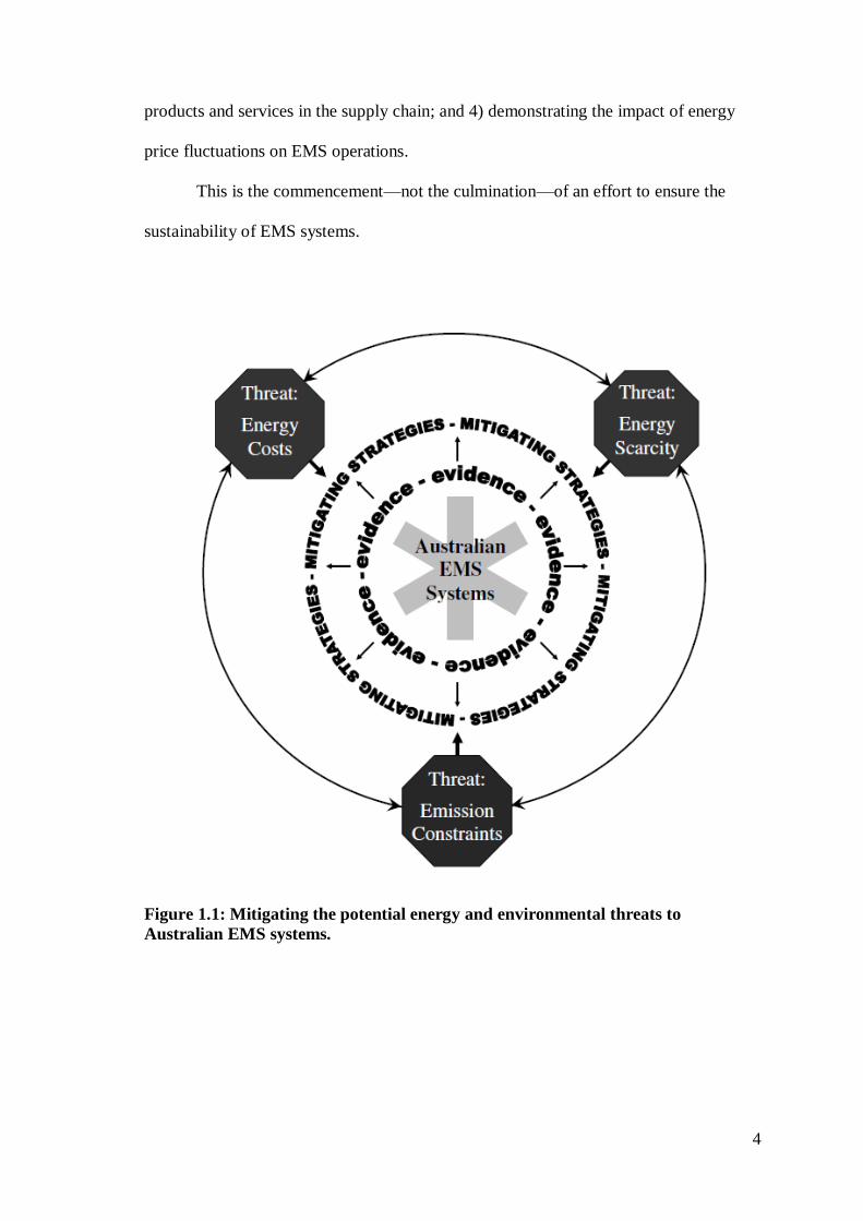
as such, are particularly vulnerable to these inter-related threats. To be successful,

strategies for mitigating these threats to EMS operations must be based on and

supported by sound evidence (Figure 1.1). Understanding the energy and environmental

burden of ambulance systems, and how these external threats manifest within those

systems, is a first step towards establishing that evidence base.

This thesis thus begins to answer the question: How can Australian EMS

systems be sustained in an economic, political, and social environment in which energy

is increasingly scarce and costly, and energy consumption is increasingly constrained

due to concerns about greenhouse gas emissions? It does this by: 1) reviewing the

extant literature on greenhouse gas emissions from health-related activities; 2)

determining the greenhouse gas emissions associated with the direct and purchased

energy consumption of EMS activities; 3) estimating the complete life cycle emissions

of Australian ambulance operations, including the upstream emissions arising from

4

products and services in the supply chain; and 4) demonstrating the impact of energy

price fluctuations on EMS operations.

This is the commencement—not the culmination—of an effort to ensure the

sustainability of EMS systems.

Figure 1.1: Mitigating the potential energy and environmental threats to

Australian EMS systems.

5

1.2 Background

1.2.1 Emergency Medical Services

Internationally, ‘EMS’ is probably the most widely recognised name for what

are also known as ‘ambulance services’ in the United Kingdom (U.K.) and Australia,

and ‘Emergency Health Services’ (EHS) in Canada. While ambulance transport is one

facet of EMS systems, their primary mission is to deliver high-quality medical care to

patients at the scene of an emergency. EMS systems are part emergency service, part

medical care, part public health, part community or social service, and (only) part

transportation service (Brown & Devine, 2008; Delbridge et al., 1998; Garrison et al.,

1997; Mann & Hedges, 2002).

For Australia’s 22 million inhabitants (and visitors), ‘ambulance services’ are

delivered as a public good by the eight State and Territory governments, either through

a government department or through a subcontract with St. John Ambulance, a private

not-for-profit organisation. In the 2009-2010 financial year, Australian ambulance

services mounted 3.5 million emergency and non-emergency responses, and transported

2.8 million patients. Operating costs for that year exceeded $2.1 billion (Council of

Ambulance Authorities, 2010).

EMS systems save lives. Out-of-hospital cardiac arrest survival rates improve

significantly when systems are optimised for rapid response and EMS personnel are

equipped with cardiac defibrillators (Stiell et al., 1999). Patients having difficulty

breathing have better outcomes when emergency personnel can give ‘breathing

treatments’ and other respiratory medications (Stiell et al., 2007). Victims of car crashes

and other trauma have higher survival rates when communities have cohesive trauma

systems, including well developed EMS systems (Liberman, Mulder, Jurkovich, &

Sampalis, 2005; Moore, Hanley, Turgeon, & Lavoie, 2010; Schiller et al., 2009).

6

Ground and air EMS systems are a critical component of the public health

infrastructure: EMS is the intersection of public safety, public health, and health care

systems (Delbridge et al., 1998). On the surface, the holistic public health perspective of

health as “…a state of complete physical, mental and social well-being and not merely

the absence of disease or infirmity” (Grad, 2002, p. 984) may seem nearly antithetical to

the episodic, emergent, patient-based nature of EMS. In fact, however, “EMS

professionals see firsthand—in people’s bedrooms and living rooms, in their cars and in

their workplaces, in neighbourhoods and communities—the interactions between

individuals, their health, economic and social circumstances, community structure and

resources, and environmental factors” (Brown & Devine, 2008, p. 109). As a result,

EMS systems can play an important role in a number of public health activities,

including elder issues (Shah, Lerner, Chiumento, & Davis, 2004; Weiss, Ernst, Miller,

& Russell, 2002), disease prevention (Lerner, Fernandez, & Shah, 2009) and disease

surveillance (National Highway Traffic Safety Administration, 2007), injury prevention

(Garrison et al., 1997), and others.

1.2.2 Are EMS Systems Vulnerable?

Sustaining EMS systems does not merely mean continuing to provide

emergency services. Indeed, it is unlikely that either economic or environmental

pressures would lead to a complete shutdown of ambulance operations in any

community. In this sense, sustaining EMS systems means continuing to provide both

the quantity and quality of services necessary to meet the public health and medical care

needs of the community. Administrative activities, recruiting and hiring, professional

development education for clinicians, and equipment maintenance are just a few

examples of non-patient care activities that might be viewed as ‘non-essential’ and thus

7

subjected to rationing as a result of constraints on energy consumption. Yet, all of these

activities, and others, are ultimately necessary to sustain the full spectrum of EMS

activities, including the delivery of high-quality patient care (Lerner, Nichol, Spaite,

Garrison, & Maio, 2007).

Given the importance of EMS systems, it might be hard to imagine that there

would be any doubt about their sustainability; surely communities would always ensure

the availability of emergency ambulance services. Around the globe, however, the lay

media regularly report cuts in ‘essential’ public services, such as: police and fire

departments (Armstrong, 2009; Booth, 2010); mental health services (Styles, 2009);

community-based HIV and AIDS service organisations (Canadian News Wire, 2009);

parks and recreation services, community centres, and even streetlights (Booth, 2010).

The medical literature also contains reports of reductions in health services and closures

of hospitals, and of the impacts of those decisions on patients and communities (Jackson

& Whyte, 1998; Probst, Samuels, Hussey, Berry, & Ricketts, 1999; Reif, DesHarnais, &

Bernard, 1999), including some reports from Australia (Farhall, Trauer, Newton, &

Cheung, 2003; Fraser, 2004). Nothing is sacrosanct.

This research focuses specifically on threats to EMS systems posed by energy

scarcity, energy costs, and constraints on greenhouse gas emissions (Figure 1.1 above).

As the following sections demonstrate, these are not simply theoretical concerns.

1.2.2(a) Energy Scarcity

In 2008, delivery of diesel and gasoline to parts of the south-eastern United

States (U.S.) was interrupted resulting in widespread fuel shortages (Associated Press,

2008; Stock & Siceloff, 2008). Although there were no published reports of disruptions

to direct patient care services, some EMS operations were affected in other ways. In

8

metropolitan Atlanta, Georgia, ambulances had to source fuel from alternative suppliers

(Hess and Greenberg, 2011); one system in North Carolina had to suspend community

and employee educational programs (personal communication, S. Hawkins, Burke

County N.C. EMS).

While episodic local, regional and national variations in energy supplies are an

immediate energy threat to EMS systems, global energy scarcity is a more challenging

and longer-term threat. The concept of ‘peak oil’ was first proposed by M. King

Hubbert in the 1950s, referring specifically to the anticipated peak for oil production in

the continental U.S. (Hubbert, 1956). The prediction was that oil production would

reach a pinnacle, and then decline rapidly. For the U.S., that peak occurred in the 1970s

with continuing energy demands met through importation of foreign oil. The concern

now is for global peak oil, when it will occur or if it already has (Aleklett et al., 2010;

Schnoor, 2007; Sorrell, Speirs, Bentley, Brandt, & Miller, 2010; Verbruggen & Al

Marchohi, 2010), and how that will directly and indirectly affect public health and

health services (Frumkin, Hess & Vindigni, 2007, 2009; Hanlon & McCartney, 2008;

Hess, Heilpern, Davis, & Frumkin, 2009; Wilkinson, 2008).

Persistent fuel shortages would impact both the breadth of services and quality

of patient care delivered by EMS systems.

1.2.2(b) Energy Costs

Throughout the developed world, EMS operations struggled to continue service

delivery during the dramatic fuel price increases experienced in 2007 and 2008. For

example, in British Columbia, Canada, price increases added $6 million to the fuel costs

of the ambulance service, a 50% increase that had not been budgeted (Penner, 2008). In

the U.S., one private corporation providing air medical services and aircraft resources in

9

44 states saw its earnings per share fall nearly 37% (Harlin, 2009). While neither of

these operations ceased providing emergency services, financial resources had to be

redirected from other activities to accommodate these fiscal insults.

A persistent need to divert resources to accommodate increased energy costs

would also impact both the breadth of services and quality of patient care delivered by

EMS systems.

1.2.2(c) Constraints on Greenhouse Gas Emissions

While it has received much more attention in recent years, global warming is not

a new concern. Since the late 1980s there have been reports of increasing global surface

temperatures amounting to 0.5oC over the 130 years between the 1850s and 1980s

(Piver, 1991). Current estimates are that, even with concerted efforts to address climate

change, global surface temperatures will continue to increase to somewhere between

2oC to 2.5

oC above pre-industrial levels (Allen et al., 2009; Ramanathan & Feng, 2008).

Political and social pressures to constrain greenhouse gas emissions will likely

intensify and, although less certain, increasing legislative and regulatory constraints on

emissions are possible. On an international basis, efforts to restrain and reduce carbon

dioxide (CO2) and other greenhouse gas emissions are escalating. Building on the

experience of the Montreal Protocol, which resulted in significant reductions in the

chlorofluorocarbons (CFCs) responsible for ozone depletion (Velders, Andersen,

Daniel, Fahey, & McFarland, 2007), the Kyoto Protocol and the more recent

Copenhagen Accord seek to limit greenhouse gas emissions and eventually reduce them

to pre-1990 levels. While the details of the limits and mechanisms for accounting

continue to be debated, there is extensive commitment to the concept with 187 countries

10

having signed and ratified the Kyoto Protocol, and 188 nations supporting the

Copenhagen Accord (Ramanathan & Xu, 2010).

Ambulance operations are motor vehicle—and aircraft—dependent; intensifying

efforts to constrain greenhouse gas emissions threatens both the breadth and quality of

services provided by EMS operations.

1.3 Specific Aims

How can Australian EMS systems be sustained in an economic, political, and

social environment in which energy is increasingly scarce and costly, and energy

consumption is increasingly constrained due to concerns about greenhouse gas

emissions? This research includes four specific aims that will help begin to answer that

question by quantifying the greenhouse gas emissions produced by Australian EMS

systems, identifying the energy sources and production processes that contribute most to

Australian ambulance service emissions, and determining how energy costs affect

Australian ambulance operations:

Specific Aim #1: Review the extant literature on the energy consumption and the

environmental impact of health services.

Specific Aim #2: Identify the primary sources of, and amount of greenhouse gas

emissions arising from, the direct and purchased energy consumption of Australian

EMS systems.

Specific Aim #3: Estimate the complete life cycle greenhouse gas emissions of

Australian EMS systems, including emissions arising from upstream activities in the

11

supply chain, and explore the production processes that might contribute most to those

emissions.

Specific Aim #4: Evaluate the historic relationships between energy costs and the

resource, operational and safety performance measures of Australian EMS systems.

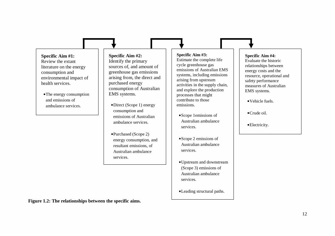
Figure 1.2 shows the relationships between the specific aims.

1.4 Assumptions

There are a number of assumptions underpinning these specific aims, and these

are explicitly stated here. This thesis does not test these assumptions:

● EMS systems are an integral component of the public health system, and have a

positive impact on health at both the population and individual patient levels

(Delbridge et al., 1998; Garrison et al., 1997; Liberman, Mulder, Jurkovich, &

Sampalis, 2005; Mann & Hedges, 2002; Schiller et al., 2009; Stiell et al., 1999;

Stiell et al., 2007).

● All of the components of EMS systems are necessary to meet their public health

and patient care objectives (Lerner, Nichol, Spaite, Garrison, & Maio, 2007).

● Mounting energy scarcity, increasing energy costs, and intensifying constraints on

greenhouse gas emissions are imminent (Aleklett et al., 2010; Ramanathan & Xu,

2010; Sorrell, Speirs, Bentley, Brandt, & Miller, 2010; Verbruggen & Al Marchohi,

2010).

12

Figure 1.2: The relationships between the specific aims.

Specific Aim #1:

Review the extant

literature on the energy

consumption and

environmental impact of

health services.

The energy consumption

and emissions of

ambulance services.

Specific Aim #3:

Estimate the complete life

cycle greenhouse gas emissions of Australian EMS

systems, including emissions

arising from upstream activities in the supply chain,

and explore the production

processes that might

contribute to those emissions.

Scope 1emissions of

Australian ambulance

services.

Scope 2 emissions of

Australian ambulance

services.

Upstream and downstream

(Scope 3) emissions of

Australian ambulance

services.

Leading structural paths.

Specific Aim #2:

Identify the primary

sources of, and amount of

greenhouse gas emissions

arising from, the direct and

purchased energy

consumption of Australian

EMS systems.

Direct (Scope 1) energy

consumption and

emissions of Australian

ambulance services.

Purchased (Scope 2)

energy consumption, and

resultant emissions, of

Australian ambulance

services.

Specific Aim #4: Evaluate the historic

relationships between

energy costs and the

resource, operational and safety performance

measures of Australian

EMS systems.

Vehicle fuels.

Crude oil.

Electricity.

13

● EMS systems are not impervious to mounting energy scarcity, increasing energy

costs or intensifying constraints on greenhouse gas emissions (Associated Press,

2008; Harlin, 2009; Hess & Greenberg, 2011; Penner, 2008; Stock & Siceloff,

2008).

● EMS systems can adapt to the evolving economic, political, and social

environment; that adaptation will be better if it is driven by evidence.

1.5 Significance

Ultimately, the results of this work can be used to help ensure both the economic

and environmental sustainability of Australian EMS systems, including the full range of

non-patient-care activities required to support high-quality service delivery. In the short

run, ambulance systems might be able to reduce administrative or ancillary activities to

accommodate constraints on energy consumption, energy expenditures or greenhouse

gas emissions; in the long run reductions in those support activities would eventually

begin to compromise patient care. Equipping systems and their leaders with empirical

data regarding EMS energy consumption and greenhouse gas emissions will enable

them to better respond to public policy initiatives designed to constrain or reduce

emissions, as well as to better manage diminished fuel availability or increasing energy

costs. The likely (and optimal) strategies for managing EMS-related energy

consumption and emissions are yet to be determined. It is unlikely that any single

strategy will work for all systems; some seemingly intuitive strategies might not fully

achieve the anticipated results, or indeed they might actually have detrimental effects—

phenomena known respectively as ‘rebound’ and ‘backfire’ (Druckman, Chitnis,

Sorrell, & Jackson, 2011; Hanley, McGregor, Swales, & Turner, 2009). Future work

14

evaluating potential energy- and emission-mitigating strategies is crucial to ensure that

any actions taken have the desired impact.

With improved knowledge of the greenhouse gas emissions associated with

EMS operations and the potential targets for emission mitigating strategies, EMS

systems can begin to develop and implement policies aimed at reducing their carbon

footprint. In the U.S. it is estimated that up to 20 million ambulance transports occur

each year (Nawar, Miska, & Xu, 2007). In Australia, the number of ambulance

responses and transports is smaller (in the order of 3 million), but many involve patients

in remote settings necessitating transport over longer distances, and often requiring air

medical transport. Given the scope of EMS operations on a global scale, even marginal

reductions in the emissions from each individual ambulance response could result in

significant overall reductions of greenhouse gas emissions.

There are also additional benefits to minimising EMS-related emissions, as their

effects have both direct and indirect impacts on EMS. Vehicle emissions are associated

with ill-health, particularly (and ironically) cardiac and respiratory diseases responsible

for many EMS responses (Gallagher et al., 2010; Jerrett et al., 2008; McConnell et al.,

2006; Medina-Ramon, Goldberg, Melly, Mittleman, & Schwartz, 2008; Modig et al.,

2006). This is also an occupational health issue; although modern engines produce

fewer pollutants, diesel fumes have been implicated in some respiratory problems

experienced by emergency personnel (Gately & Lenehan, 2006).

Further, while the current popular emphasis might be on reducing EMS-related

greenhouse gas emissions and their contribution to global warming, the real ‘win’ from

managing those emissions is likely to be a reduction in energy consumption, and thus

energy costs. With improved knowledge of the predominant energy burdens of EMS

systems, the relative energy demands of different EMS delivery models can be

15

considered when developing and revising system operational models, and policies can

be designed and implemented to reduce energy consumption and energy-related costs.

1.5.3 Potential Broader Impact

The results of this work, while specific to Australian EMS systems, could also

prove beneficial to EMS operations in other countries as well as to other areas of public

health. There is increasing interest in the emissions associated with health activities

(Anonymous, 2008; Bayazit & Sparrow, 2010; Blakemore, 2009; Blanchard & Brown,

2009; 2011; Callister & Griffiths, 2007; Chung & Meltzer, 2009; Creagh, 2008;

Gilliam, Davidson, & Guest, 2008; Hudson, 2008; Mayor, 2008; McMichael &

Bambrick, 2007; Roberts & Godlee, 2007; Somner, Scott, Morris, Gaskell, & Shepherd,

2009; Somner et al., 2008), and this work could contribute to those efforts. The results

of this work could also inform broader economic and environmental efforts related to

the sustainability of health care systems, serving as a foundation for future studies.

Although it is not the focus of this work, the methods developed and findings could be

particularly useful in efforts to develop health services—particularly ambulance

services—in resource poor environments, where energy scarcity is already impeding

public health.

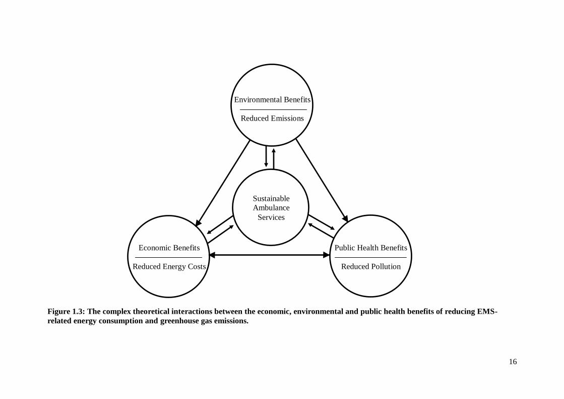
The relationships between the environment, economic forces, and health

services are multifaceted and often unclear. Figure 1.3 is a hypothetical representation

of the complex theoretical interactions between the environmental, economic and public

health benefits of reducing EMS-related energy consumption, energy expenditures and

greenhouse gas emissions.

16

Figure 1.3: The complex theoretical interactions between the economic, environmental and public health benefits of reducing EMS-

related energy consumption and greenhouse gas emissions.

Economic Benefits

Reduced Energy Costs

Public Health Benefits

Reduced Pollution

Environmental Benefits

Reduced Emissions

Sustainable

Ambulance

Services

17

Chapter 2: Theoretical and Methodological Framework

This chapter lays out the theoretical and empirical bases for climate change,

energy scarcity and energy costs, and reviews the methodological approaches to

inventorying energy consumption and greenhouse gas emissions.

2.1 Climate Change

2.1.1 Atmospheric Temperatures Are Increasing

In the late 1980s Hansen & Lebedeff (1987; 1988) analysed monthly surface air

temperature data from three partially overlapping data sources: the U.S. National Center

for Atmospheric Research, the National Oceanic and Atmospheric Administration

(NOAA) “Monthly Climatic Data of the World” and the NOAA monthly mean station

records. They found the 1980s to be the warmest decade in the history of instrument-

measured temperatures, with the four warmest years on record occurring in that decade

(Hansen & Lebedeff, 1987; 1988). They also found that the rate of warming between

the mid-1960s and late 1980s was greater than that which occurred between the 1880s

and 1940s. After correcting for ‘heat island’ effects of increasing urbanisation, they

estimated the 1987 global surface temperature was 0.63 + 0.2oC warmer than in 1880

(Hansen & Lebedeff, 1988).

Using completely different methods, Urban, Cole & Overpeck (2000) reached

remarkably similar conclusions. They evaluated core samples from coral growing on the

outer reef at Maiana Atoll in Kiribati using mass spectrometry with the isotope δ18

O to

create a 155-year climate record dating from 1840 to 1995. They found a trend towards

increasingly warmer and wetter conditions spanning the full record, with gradual

increases in the early twentieth century followed by abrupt changes after 1976. Further,

they found increasing climate volatility, with climate variability occurring primarily on

18

a decadal scale in the early record, but on a mainly inter-annual scale in the twentieth

century.

Increasing surface temperatures continued through the 1990s and early 2000s. In

the 4th report of the Intergovernmental Panel on Climate Change (IPCC), the “Physical

Science Basis” working group reviewed data from four distinct evaluations, finding that

between 1979 and 2005 mean surface temperatures increased between 0.19 ± 0.07oC to

0.32 ± 0.09oC per decade, with the differences in estimations attributed primarily to

differences in approaches to spatial averaging (Solomon et al., 2007).

2.1.2 Greenhouse Gases Collect in the Atmosphere

‘Greenhouse gases’ are components of the Earth’s atmosphere that allow light

to easily penetrate the atmosphere and warm the planet’s surface; they also absorb, hold

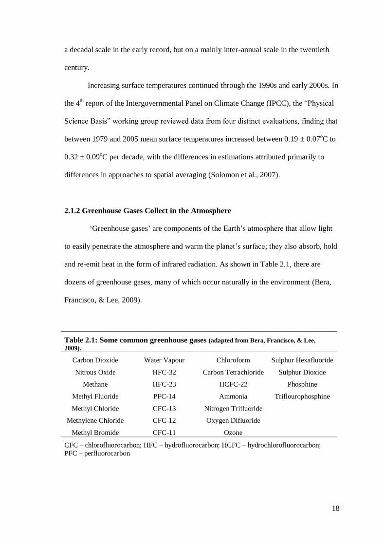
and re-emit heat in the form of infrared radiation. As shown in Table 2.1, there are

dozens of greenhouse gases, many of which occur naturally in the environment (Bera,

Francisco, & Lee, 2009).

Table 2.1: Some common greenhouse gases (adapted from Bera, Francisco, & Lee,

2009).

Carbon Dioxide Water Vapour Chloroform Sulphur Hexafluoride

Nitrous Oxide HFC-32 Carbon Tetrachloride Sulphur Dioxide

Methane HFC-23 HCFC-22 Phosphine

Methyl Fluoride PFC-14 Ammonia Triflourophosphine

Methyl Chloride CFC-13 Nitrogen Trifluoride

Methylene Chloride CFC-12 Oxygen Difluoride

Methyl Bromide CFC-11 Ozone

CFC – chlorofluorocarbon; HFC – hydrofluorocarbon; HCFC – hydrochlorofluorocarbon;

PFC – perfluorocarbon

19

Greenhouse gases are not inherently bad. As Grenfell et al. (2010, p. 77)

explain, “Without greenhouse-like conditions to warm the atmosphere, our early planet

would have been an ice ball, and life may never have evolved”. The atmosphere as we

know it today is the product of complex interactions between early bacterial life forms

that produced and consumed oxygen, photosynthesis, and greenhouse effects (Grenfell

et al., 2010).

Different greenhouse gases have different heat absorbing, holding and emitting

characteristics and thus different ‘global warming potentials’ (GWP) (Bera, Francisco,

& Lee, 2009; Hansen et al., 1998). CO2 is the most abundant of the greenhouse gases,

and is the reference against which other greenhouse gases are measured. CO2 has a

GWP of 1, and other greenhouse gases are measured as CO2 equivalents (CO2e).

Methane (CH4), for example, has a GWP about 25 times that of CO2, or a GWP of 25

CO2e (Bera, Francisco, & Lee, 2009).

Atmospheric levels of CO2 have risen steadily over the last millennium. For the

pre-industrial timeframe, spanning the years 1000 to 1750, the IPCC estimates

atmospheric CO2 concentrations ranged between 275 to 285 parts per million (ppm)

(Solomon et al., 2007). In the industrial age, atmospheric CO2 concentrations have risen

dramatically. Piver (1991) cites data from the Mauna Loa Observatory in Hawaii

showing an increase in atmospheric CO2 concentrations from approximately 316 ppm in

1958 when the first measurements were made to 347 ppm in 1986. In 2005, atmospheric

CO2 concentrations reached 379 ppm (Solomon et al., 2007), and in 2010

concentrations as high as 390 ppm were measured at the Mauna Loa Observatory

(National Oceanic and Atmospheric Administration, 2010).

20

2.1.3 The Association between Rising CO2 Levels and Increasing Temperatures is

Probably more than Coincidence

Rising surface temperatures and increasing atmospheric CO2 levels could co-

exist without one necessarily causing the other. There is some probability that the

association is simply a function of chance, but that probability is small.

Genthon et al. (1987) have made estimates of historic temperatures and

atmospheric CO2 levels going back 160,000 years by analysing air trapped in the

Vostok ice core from Antarctica. They conducted multivariable analysis examining the

relationship between the Vostok isotope temperature record and climatic inputs

including southern hemisphere ‘insolation’ (solar radiation of the Earth’s surface, also

referred to as ‘orbital forcing’), northern hemisphere insolation, ocean ice volume

estimated by the δ18

O deep sea record, and CO2 levels. The various models analysed

achieved high correlation, with r2 values ranging from 0.84 to 0.90. While measures of

insolation were associated with temperature increases, when holding the southern

hemisphere inputs constant and evaluating northern hemisphere forcing “[t]he common

feature of all these analyses [was] that the main contribution [came] from CO2…”

(Genthon et al., 1987, p. 416). Modifying the timescale to put it in phase with historic

sea surface temperatures around Antarctica, or limiting the analysis to the most recent

100,000 years, did not significantly change the results. Two models, both using the δ18

O

ice volume record (instead of insolation) as the northern hemisphere input, did result in

less pronounced associations between CO2 levels and the measured temperature change,

but CO2 levels still accounted for 27% to 35% of the temperature variance in both of

those models.

The authors concluded that the maximum influence of southern hemisphere

insolation inputs on temperature change is 20%, northern hemisphere inputs only

21

predominate when the ice volume record is the basis for estimates, and the relative

contributions of CO2 to temperature changes exceed 50%—and are as high as 84%—

except for when ice volume is used as the northern hemisphere input. They asserted that

“… the Vostok series appear to provide the most direct support so far of … an

interaction between CO2, orbital forcing and climate…” (Genthon et al., 1987, p. 418)

but they also caution that extrapolating analyses of past conditions to present day or

future impacts of CO2 would require a better understanding of the mechanisms involved

in this interaction.

2.1.4 Human Activity Produces Greenhouse

Human activity produces CO2 and other greenhouse gases. The greatest source

of these ‘anthropogenic’ emissions is the burning of fossil fuels including coal, oil and

its derivatives, and natural gas. The most abundant greenhouse gases influenced by

human activity are CO2, CH4, nitrogen oxide (N2O) and CFC 11 and 12 (Hansen et al.,

1998). The concern about anthropogenic greenhouse gases is not that they exist and

accumulate in the atmosphere, but rather the increasing levels at which they exist and

are accumulating in the atmosphere.

2.1.5 The Association between Rising CO2 Levels and Human Activity is Probably

more than Coincidence

Natural processes, such as volcanoes, also produce greenhouse gases, and—as

with all things in nature—there is inherent variation in atmospheric CO2 levels. It is

difficult, however, to ascribe recent atmospheric CO2 concentrations approaching 400

ppm to natural processes and inherent variation alone. For example, in the CO2 record

of the Vostok ice core, at no point did historic CO2 levels exceed 300 ppm, and to find

22

CO2 concentrations exceeding 275 ppm requires looking back more than 115,000 years

(Barnola, Raynaud, Korotkevich, & Lorius, 1987).

The predominant scientific and political consensus is that human activity, rising

CO2 levels and increasing temperatures are all inter-related. While the 15th Conference

of the Parties of the United Nations Framework Convention on Climate Change, held in

Copenhagen, Denmark in December 2009, failed to achieve agreement on how to

mitigate climate change, all but five of the 193 participating nations supported the

‘Copenhagen Accord’. The opening paragraph of the Accord states, “We underline that

climate change is one of the greatest challenges of our time” and the second paragraph

follows with, “We agree that deep cuts in global emissions are required…”

(Ramanathan & Xu, 2010, p. 8055). A lack of agreement on how to mitigate climate

change is not a lack of agreement about the relationship between anthropogenic

greenhouse gases, rising atmospheric CO2 levels, and global warming. Even with

concerted efforts to reduce greenhouse gas emissions, global surface temperatures will

likely continue to increase to between 2oC to 2.5

oC above pre-industrial levels (Allen et

al., 2009; Matthews, Gillett, Stott, & Zickfeld, 2009; Ramanathan & Feng, 2008). An

increase as large as 3.9oC to 4.3

oC above pre-industrial levels is within the 95%

confidence intervals for these estimates (Allen et al., 2009; Ramanathan & Feng, 2008).

2.1.6 A Caveat: Nothing is Absolute

It is important to recognise that the relationships between human activity,

greenhouse gas emissions and rising temperatures are neither simple nor isolated.

Rising CO2 levels and increasing temperatures are not exclusively attributable to human

activity (Hansen et al., 1998; Raschke, 2001) and some emissions from human

activity—for example, aerosols and anthropogenic clouds (e.g., aircraft contrails)—

23

actually have a cooling effect (Hansen et al., 1998; Ramanathan & Feng, 2008). Indeed,

a paradox is that reducing aerosols and other atmospheric pollutants might enhance

global warming.

There are also some who question the validity and reliability of climate data,

climate-related analyses, and even the objectivity of the peer-reviewed literature

(Robinson, Robinson, & Soon, 2007; Singer, 2003). Consensus is not 100% agreement;

association is not necessarily cause-and-effect; probability is not certainty.

The United Nations Environment Programme recognises this lack of certainty,

and has addressed it in the Rio Declaration on Environment and Development by

adopting ‘Principle 15’:

“In order to protect the environment, the precautionary approach shall be widely

applied by States according to their capabilities. Where there are threats of

serious or irreversible damage, lack of full scientific certainty shall not be used

as a reason for postponing cost-effective measures to prevent environmental

degradation” (United Nations Environment Programme, 1992).

Although not technically correct, this is sometimes referred to as ‘The

Precautionary Principle’. Put simply, in the absence of absolutely conclusive evidence,

there is greater risk in presuming rising temperatures, increasing CO2 levels, and human

activity are not interrelated; it is safer to trust the preponderance of the evidence and

take action on the presumption that they are linked.

24

2.2 Energy Scarcity

Sheikh Zaki Yamani, the Saudi Arabian oil minister between 1962 and 1986, is

quoted as saying, “The Stone Age did not end for lack of stone, and the Oil Age will

end long before the world runs out of oil” (Wilkinson, 2008, p. 664). That prediction

was about relative—not absolute—scarcity; that eventually we would consume oil

faster than we could cost-efficiently pump it out of wells, and therefore we would find

and develop other energy resources long before we ran out of oil.

2.2.1 Peak Oil

As mentioned in Chapter 1, the concept of peak oil was first described by M.

King Hubbert in the 1950s. He predicted U.S. oil production would peak in the 1970s,

and then rapidly decline. Although the high point of U.S. oil production exceeded

Hubbert’s estimate by 600 million barrels per year, the peak and subsequent fall in

production did in fact occur. That is, in 1970 U.S. oil production peaked at

approximately 3.5 billion barrels per year; it has declined ever since and by 2007 it had

dropped to less than 2 billion barrels per year (Verbruggen & Al Marchohi, 2010).

Despite recent innovations in extractions from oil shale and oil sands, the concern now

is about global peak oil (Aleklett et al., 2010; Sorrell, Speirs, Bentley, Brandt, & Miller,

2010; Verbruggen & Al Marchohi, 2010), and how that could affect public health and

health services (Frumkin, Hess, & Vindigni, 2007; Hanlon & McCartney, 2008; Hess,

Heilpern, Davis, & Frumkin, 2009; Wilkinson, 2008).

Globally, there are currently about 70,000 producing oil fields, but just 25 of

these fields account for 25% of world oil production, and a mere 500 fields hold two-

thirds of all cumulative oil discoveries (Sorrell, Speirs, Bentley, Brandt, & Miller,

2010). These are mostly older fields that have passed or are near their production peak

25

(Sorrell et al., 2010). Noting that “[a]t some point, the additional production from small

fields that are discovered relatively late will become insufficient to compensate for the

decline in production from large fields…” (Sorrell et al., 2010, p. 5290), scientists at the

U.K. Energy Research Centre undertook a systematic review of the evidence concerning

global oil depletion that included more than 500 studies, 14 global supply forecasts, and

data from industry databases (Sorrell et al., 2010). They reported that the current

estimate for the ultimately recoverable resources for conventional oil is between 2,000

and 4,300 billion barrels; this compares to cumulative production of 1,128 billion

barrels through the end of 2007. That is, what we have already consumed is equivalent

to between 25% and 50% of all currently available conventional oil. These authors

reported that the average rate of decline in production from post-peak fields is 6.5% per

year, with an average decline in production for all currently producing wells of 4% per

year. They suggested that as much as 20 billion barrels of oil must be added to global

reserves every year just to offset this decline in production. They concluded that “… a

peak of conventional oil production before 2030 appears likely and there is a significant

risk of a peak before 2020” (Sorrell et al., 2010, p. 5294). They further argued that

“[d]elaying the peak beyond 2030 requires optimistic assumptions about the size of the

recoverable resource and the rate at which it is developed…” (Sorrell et al., 2010, p.

5293).

Others are even more pessimistic. In a critical analysis of the 2008 World

Energy Outlook (WEO), which is published each year by the International Energy

Agency (IEA), Aleklett et al. (2010) evaluated the IEA estimates of future energy

consumption and production through the end of year 2030. WEO 2008 estimates

economic growth at 3% per year until 2015, corresponding to a 1.3% annual increase in

oil consumption which then falls to 0.8% per year after that. This translates into global

26

consumption of 106.4 million barrels of oil per day by 2030, which is 5.1 million

barrels per day more than the WEO 2008 production projections for that year.

These authors also made their own estimate of year 2030 oil production, taking

into consideration currently producing fields (70.2 million barrels per day in 2007) with

a rate of decline of 3.2% annually, known fields yet to be developed (257 billion barrels

by 2030), fields yet to be found (estimated by IEA at 114 billion barrels by 2030) and

emerging innovative technologies for recovering non-conventional oils including oil

sands, heavy oil from Venezuela, ‘gas-to-liquids’ and ‘coal-to-liquids’, chemical

additives, and natural gas liquids. They also factored in the potential for enhanced oil

recovery technologies. Still, they estimated 2030 production at only 75.8 million barrels

per day—nearly 25% less than the WEO 2008 estimate (Aleklett et al., 2010).

The differences in all of these estimates are primarily attributable to the

predicted depletion rate of remaining recoverable resources. That is, as the remaining

volume of oil in any given field goes down, how much of that remaining oil can

efficiently be recovered each year? This varies by type of well, and presumably new

technologies will drive depletion rates higher, but the WEO 2008 estimates of future on-

shore oil well depletion rates in the 9% to 15% range by 2025-2030 far exceed anything

achieved so far (~2% to 7%). Thus, as Aleklett et al. (2010, p. 1412) concluded, future

oil production is unlikely to meet future demand as estimated by WEO 2008; “[t]he

world appears most likely to have passed the peak of global oil production and to have

entered the descent phase” [emphasis added].

Of course, predictions of future oil supplies and production, whether optimistic

or pessimistic, are inherently imperfect. They are based on “…the amount of oil that is

mineable at today’s prices using existing technology” (Verbruggen & Al Marchohi,

2010, p. 5576) and are subject to frequent revision. For example, IEA projections have

27

been described as “… alternating from optimistic to pessimistic and back again”

(Miller, 2011, p 1569). These variations primarily result from changes in the

assumptions underlying the predictions, particularly those related to economic growth

and consumption as well as technological advancements in the recovery processes

(Miller, 2011; Verbruggen & Al Marchohi, 2010). Also, one cannot completely

discount that political or proprietary interests might also influence the predictions.

2.2.2 Peak Minerals or Peak Resources

Oil is not the only energy source at risk of relative scarcity. More recently,

authors have raised the spectre of impending ‘peak coal’ (Heinberg & Fridley, 2010;

Mason, Prior, Mudd, & Giurco, 2011; Patzek & Croft, 2010), as well as peak

production for other minerals (Mason, Prior, Mudd, & Giurco, 2011), and how that

might affect electricity production. Scarcity of rare earth minerals could potentially

even constrain deployment of solar- and wind-generated electricity technologies.

2.2.3 Opposing Perspectives

Not everyone accepts that peak oil (or peak minerals/resources) is inevitable.

Radetzki (2010, p. 6566) cites past “[p]rophecies of impending catastrophes based on

resource pessimism” and argues that since “none of them have actually occurred”

human ingenuity, technical progress and competitive markets can adequately address

the problem. He argues that estimates of ultimately recoverable reserves are

continuously updated, and that oil fields invariably produce more oil than is estimated

when they are first discovered. Radetzki (2010, p. 6569) slightly misquotes a decade-old

passage by Adelman (2002) to make his point:

28

“In 1944, world proved reserves were 51 billion barrels. In 1945-1998, 605

billion barrels were removed, leaving 1035 billion” (Adelman, 2002, p. 180).

However, Adelman (2002) also argued that ‘nonproved reserves’ (or fields yet

to be found)…

“…are not comparable with or additive to proved reserves. They are estimated

future output from facilities not yet in being, whose costs will reflect future

geology and engineering. Anyone who adds nonproved to proved reserves, and

from that total predicts future output, implicitly claims to know future science

and technology” (Adelman, 2002, p. 180).

Presumably, then, he would disagree with Radetzki’s reliance on anticipated

future reserves and production as protection against peak oil. Indeed, Adelman didn’t

argue against peak oil, but rather (much like Sheikh Yamani) predicted economic

scarcity driven by constraints on production in the form of rising marginal costs, not

absolute scarcity.

Verbruggen & Al Marchohi (2010) also discussed the limitations of estimating

future oil production, noting that today’s technologies leave nearly two-thirds of a

field’s oil in the ground. Oil shortages will likely drive up prices and spur innovation

such that in the future oil field production, rate of decline, and the depletion rate of

remaining recoverable resources will be more advantageous than today. They also point

out that projections of peak oil are hampered by inconsistencies in the definitions used

for ‘conventional oils’, ‘non-conventional oils’, ‘reserves’ and ‘resources’, and by

physical, economic, and technological uncertainties—particularly in less developed

29

nations. They do not question the concept of peak oil, but they note that current

predictions are really about “…the peaking of conventional, easy-to-access ‘premium’

oil, not too far in the future” (Verbruggen & Al Marchohi, 2010, p. 5578). That is, a

step along the way to peak oil is ‘peak cheap oil’.

Economic and environmental pressures on energy consumption are also inter-

related, and growing environmental concerns could suppress oil production more so

than limited supply or constraints on production (Verbruggen & Al Marchohi, 2010).

Thus,

“[t]he insight is growing that we will (have to) leave many oil resources in the

ground because the transition to highly efficient, renewable energy based energy

economies is urgent. So a peak in oil production may actually be observed in the

next decade, not because of oil reserves shortage but because of scarcity of

atmospheric space for dumping carbon dioxide from oil winning and oil

combustion” (Verbruggen & Al Marchohi, 2010, p. 5580).

2.3 Energy Costs

Energy scarcity is only one of the energy-related threats to health systems.

Energy costs are an equally important, and potentially more pressing, concern for health

services, including EMS.

2.3.1 Energy Costs and Economic Performance

Energy costs vary widely over time, and are affected by a complex and difficult

to model interplay between world events, production levels, consumer demand, political

sensitivities and tax policies (Gallo, Mason, Shapiro, & Fabritius, 2010; Ghoshray &

Johnson, 2010; Hamilton, 1983). On a macroeconomic level, sharp increases in oil

30

prices are a precursor to slowing in the growth of gross national product in the U.S., and

have pre-dated every recession in that nation since World War II except for one (1960-

1961) (Hamilton, 1983). Oil and energy price shocks, as well as price volatility, also

adversely affect stock returns in market economies around the world (Faff & Brailsford,

1999; Huang, Hwang, & Peng, 2005; Jones & Kaul, 1996; Nandha & Faff, 2008; Park

& Ratti, 2008; Sadorsky, 1999), although energy stocks do benefit from price shocks

(El-Sharif, Brown, Burton, Nixon, & Russell, 2005; Huang, Masulis, & Stoll, 1996).

The negative impacts of price shocks on stock returns are greatest for medium-sized

firms (Sadorsky, 2008). Energy price increases and price volatility also negatively

impact firm-level strategic investment (Henriques & Sadorsky, 2011; Yoon & Ratti,

2011). Firms that undertake sustainability initiatives, however, generally reduce their

exposure to energy price fluctuations (Henriques & Sadorsky, 2010).

There is also some evidence that energy costs contribute to health care price

inflation. A time series analysis of U.S. petroleum and health care prices between 1973

and 2008 found a 1% increase in oil price inflation was associated with a 0.03%

increase in medical care prices after an eight month lag. This price elevation persisted

for 20 months, although the effect was much stronger in the 1970s than in recent years.

(Hess, Bednarz, Bae, & Pierce, 2011).

2.4 Energy Consumption and Emissions Accounting Methodologies

There are a number of approaches to energy and emissions accounting; these are

described in the following sections.

2.4.1 Ecological Footprints

One measure of environmental impact is the ‘ecological footprint’, which Rees

(1992, p. 121) described as “the total area of land required to sustain [a] … region”.

31

Ecological footprints express the consumption and waste associated with human

economic activity in terms of the hectares of land required to provide the resources

necessary to support that activity as well as absorb the waste generated by that activity

(Kitzes & Wackernagel, 2009; Rees, 1992). It is not a perfect, universally applied

metric (Moffatt, 2000; Templet, 2000; van den Bergh & Verbruggen, 1999)—for

example, there is some debate as to whether an ecological footprint should be measured

in terms of local hectares and thus the carrying capacity of only the land geographically

proximal to the economic activity, or in terms of global hectares and thus the entire

carrying capacity of the Earth (Wackernagel, Monfreda, Erb, Haberl, & Schulz, 2004;

Wiedmann & Lenzen, 2007). Still, conceptually the ecological footprint is seen as at

least a useful metaphor in sociological and political discussions (Opschoor, 2000; van

Kooten & Bulte, 2000), and environmentalists and ecologists continue to use and

improve the measure to describe the sustainability of human activities (Kitzes et al.,

2009; Wackernagel, 2009). It has been used in studies evaluating the environmental

burden of, for example, the New Zealand economy (Bicknell, Ball, Cullen, & Bigsby,

1998), academic departments within a University (Wood & Lenzen, 2003), the

economies of Austria, the Philippines and South Korea (Wackernagel et al., 2004), the

province of Siena, Italy (Bagliani, Galli, Niccolucci, & Marchettini, 2008) and grain

consumption in Israel (Kissinger & Gottlieb, 2010).

2.4.2 Carbon Footprints

Recently, the term ‘carbon footprint’ has gained colloquial traction as a moniker

for the environmental impact of an entity or activity. ‘Carbon footprint’ is likely derived

from the term ‘ecological footprint’ (Matthews, Hendrickson, & Weber, 2008).

Although it has no universally accepted definition, generally a carbon footprint is an

32

accounting of the CO2 and other greenhouse gases emitted by an organisation over some

period of time (Matthews et al., 2008; Purman, 2008), usually measured in tonnes (t) of

CO2 or, for other greenhouse gases, as CO2e representing their atmospheric warming

potential using a common denominator. Thus, it differs from the ecological footprint in

that it does not characterise activities in the explicit context of the carrying capacity of

Earth, but rather in the implicit context of the carrying capacity of Earth’s atmosphere.

2.4.2(a) The Scopes of Carbon Footprints

There is considerable variability in the approaches taken to carbon footprinting

(Kenny & Gray, 2009; Pandey, Argrawal, & Pandey, 2011). Regardless of how energy

consumption and emissions are inventoried, though, carbon footprints are typically

described in terms of three ‘scopes’.

Scope 1 Emissions: The emissions associated with the petrol and diesel

consumed to operate an organisation’s vehicle fleet would be an obvious component of

that organisation’s carbon footprint. Equally apparent would be the emissions associated

with burning natural gas, fuel oil, kerosene or other fuels in furnaces or, perhaps, in on-

site generators that produce electricity. Accounting for these types of direct energy

consumption and their resultant emissions is classified as a Scope 1 carbon footprint

(Australian Government Department of Climate Change, 2009a; Matthews,

Hendrickson, & Weber, 2008; Purman, 2008).

Scope 2 Emissions: Less obvious, but equally logical, is to include the emissions

associated with purchased energy in an organisation’s carbon footprint. The most

common example is emissions associated with electricity generation. Although using

electricity to power equipment in a factory or office doesn’t produce emissions directly

from that factory or office, the process of generating that electricity—typically in coal-

33

fired power plants—does produce emissions. Organisations should account for the

emissions that result from generating the electricity they consume. Although somewhat

rare in the modern world, the same would be true for organisations that utilise

municipally-generated piped-in steam. A more common—and often overlooked—

example is the emissions associated with employees’ work-related commercial air (or

rail) travel. Accounting for these types of indirect purchased energy consumption and

their resultant emissions is classified as a Scope 2 carbon footprint (Australian

Government Department of Climate Change, 2009a; Matthews, Hendrickson & Weber,

2008; Purman, 2008).

Scope 3 Emissions: Scope 3 carbon footprints account for the ‘upstream’

emissions that arise from producing the supplies and equipment used by an

organisation, as well as the ‘downstream’ emissions associated with disposing of the

waste generated by that organisation and its products or services (Australian

Government Department of Climate Change, 2009a; Lenzen, Murray, Sack, &

Wiedmann, 2007; Matthews, Hendrickson, & Weber, 2008; Purman, 2008; Ross &

Evans, 2002). In terms of products and processes that are only one or two steps away

from an organisation’s final product or service, the concept isn’t outlandish: it is

reasonable that a freight company would account for the emissions associated with

manufacturing the tyres used on its trucks, or that a hospital would account for the

emissions associated with commercial laundering of its linens. A true Scope 3 analysis,

however, goes further. For example, a hospital would also account for a pro-rata portion

of the emissions associated with manufacturing the tires used on the delivery vans of the

commercial laundry that providers its linen service, and so forth.

Complete Life Cycle Emissions: Although the phrase ‘Scope 3 carbon footprint’

is sometimes used synonymously with ‘complete life cycle’ carbon footprint, a

34

‘complete life cycle’ carbon footprint is actually the sum of Scope 1, Scope 2 and Scope

3 emissions. The concept behind Scope 3 carbon footprints and life cycle analysis is

important from two perspectives. First, the fossil energy consumption and related

emissions represented in Scope 1 and Scope 2 carbon footprints do not adequately

characterise the environmental impact of most products and services (Huijbregts et al.,

2006; Matthews, Hendrickson, & Weber, 2008; Purman, 2008). Second, if upstream and

downstream impacts are not considered in an organisation’s carbon footprint, emission

reduction strategies could lower Scope 1 and Scope 2 emissions while total emissions

from upstream or downstream processes actually rise. The direct emissions resulting

from the organisation’s activities would decrease, but total emissions into the

atmosphere—the ultimate target of greenhouse gas mitigation efforts—would increase.

One striking example of how reductions in Scope 1 emissions can be misleading is bio-

fuels. While the exact impacts vary by both the source material (for example, corn vs.

switch-grass) and production processes, in many cases the reduction in direct carbon

emissions that results from using bio-fuels instead of fossil fuels is more than offset by

the emissions associated with cultivating the plant stock and refining it into fuel, as well

as by the resultant land use changes that can affect both ecosystems and food chains

(Coronada, de Carvalho, & Sliveira, 2009; Gnansounou, Dauriat, Villegas, & Panichelli,

2009; Huo, Wang, Bloyd, & Putsche, 2009; Lange, 2011; Lapola et al., 2010; Reijnders,

2011; Searchinger et al., 2008; Solomon, 2010).

The International Organisation for Standardisation (ISO) addresses life cycle

analyses in two standards: ISO 14040 and ISO 14044, identifying seven principles of

life cycle analysis (Table 2.2) (Finkbeiner, Inaba, Tan, Christiansen, & Kluppel, 2006).

One key point is that the complexity of and varying approaches to life cycle analysis

make comparisons between the carbon footprints of individual organisations perilous.

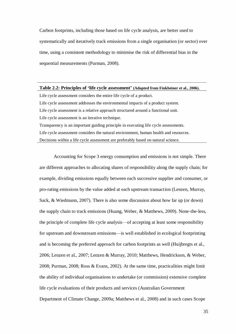
35

Carbon footprints, including those based on life cycle analysis, are better used to

systematically and iteratively track emissions from a single organisation (or sector) over

time, using a consistent methodology to minimise the risk of differential bias in the

sequential measurements (Purman, 2008).

Table 2.2: Principles of ‘life cycle assessment’ (Adapted from Finkbeiner et al., 2006).

Life cycle assessment considers the entire life cycle of a product.

Life cycle assessment addresses the environmental impacts of a product system.

Life cycle assessment is a relative approach structured around a functional unit.

Life cycle assessment is an iterative technique.

Transparency is an important guiding principle in executing life cycle assessments.

Life cycle assessment considers the natural environment, human health and resources.

Decisions within a life cycle assessment are preferably based on natural science.

Accounting for Scope 3 energy consumption and emissions is not simple. There

are different approaches to allocating shares of responsibility along the supply chain; for

example, dividing emissions equally between each successive supplier and consumer, or

pro-rating emissions by the value added at each upstream transaction (Lenzen, Murray,

Sack, & Wiedmann, 2007). There is also some discussion about how far up (or down)

the supply chain to track emissions (Huang, Weber, & Matthews, 2009). None-the-less,

the principle of complete life cycle analysis—of accepting at least some responsibility

for upstream and downstream emissions—is well established in ecological footprinting

and is becoming the preferred approach for carbon footprints as well (Huijbregts et al.,

2006; Lenzen et al., 2007; Lenzen & Murray, 2010; Matthews, Hendrickson, & Weber,

2008; Purman, 2008; Ross & Evans, 2002). At the same time, practicalities might limit

the ability of individual organisations to undertake (or commission) extensive complete

life cycle evaluations of their products and services (Australian Government

Department of Climate Change, 2009a; Matthews et al., 2008) and in such cases Scope

36

1 and Scope 2 emissions inventories (with an acknowledgement that Scope 3 emissions

are not accounted for) can still be useful.

2.4.3 Conducting Energy Consumption and Emissions Inventories

2.4.3(a) Approaches

There are three general approaches to conducting emissions inventories:

Bottom-up approaches identify each step or process involved in producing a

product or delivering a service—and preferably all of the upstream and downstream

components of each step or process—and explicitly measure the associated energy

consumption and greenhouse gas emissions. In a bottom-up approach, it is reasonably

easy to identify the emissions associated with, for example, electricity used to power a

factory or fuel consumed by delivery vans. Thus, the bottom-up approach is widely used

in determining Scope 1 and Scope 2 carbon footprints. Conversely, a bottom-up

approach to identifying upstream emissions requires access to significant amounts of

data about the operations of potentially hundreds or thousands of firms and

organisations in the supply chain, making a bottom-up approach to a complete life cycle

assessment a truly daunting, if not impossible, task (Hamilton, Kellet, & Yuan, 2008).

Top-down approaches typically identify the total emissions associated with

economic activities at some aggregate scale—an economic sector, a region, a nation,

etc.—and then allocates a share of those emissions to an individual firm or organisation

through some pro-rating technique such as by market share or proportion of gross

domestic product. Top-down approaches inherently include complete life cycle

emissions, but they assume that emission intensity—emissions per unit of product or

service delivered or per unit of economic activity—is constant across all firms or

37

organisations within the parent sector, region or nation (Hamilton, Kellet, & Yuan,

2008; Turner, Lenzen, Wiedmann, & Barrett, 2007).

Hybrid life cycle analyses recognise the relative strengths and shortcomings of

bottom-up and top-down methods of emissions inventories, and attempt to provide a

more complete accounting of an organisation’s emissions by combining aspects of both.

For those aspects of the organisation’s activities that lend themselves to explicit

measurement of their energy burden and emissions, a bottom-up approach is employed.

For those aspects of the organisation’s activities for which explicit energy consumption

and emissions data cannot practicably be obtained, a top-down approach is used

(Hamilton, Kellet, & Yuan, 2008; Stromman, Peters, & Hertwich, 2009; Suh, 2004).

One important caveat in hybrid life cycle analyses, however, is to ensure that emissions

are not double-counted; that is, to ensure that any emissions explicitly measured in the

bottom-down component are not included in (or are deducted from) aggregate emissions

incorporated into the top-down portion of the analysis (Stromman et al., 2009; Suh,

2004).

2.4.3(b) Input-Output Analysis

A well-established methodological approach to identifying and allocating

upstream and downstream emissions when conducting top-down and hybrid life cycle

analyses is the use of input-output analysis. Input-output analysis was developed by the

economist Wassily Leontief (who won the Nobel Prize in economics for that work) as a

way to use matrix algebra to measure and model transactions between all of the sectors

of an economy, and thus the upstream and downstream economic flows that result from

the transactions of any given sector (or firm within a sector). In1970, he described how

pollution, as a by-product of economic activity, could be incorporated into input-output

38

models and showed that such models could then subsequently be used to evaluate how

changes in one economic activity might affect cumulative pollution from all of the

upstream and downstream points in the supply chain (Leontief, 1970). Since then, input-

output analysis has been widely incorporated into analyses of energy consumption and

environmental impacts (de Haan & Keuning, 1996; Herendeen, 1978; Turner, Lenzen,

Wiedmann, & Barrett, 2007; Wiedmann, Minx, Barrett, & Wackernagel, 2006),

including for example the environmental impacts of: economic sectors within national

economies (Cadarso, Lopez, Gomez, & Tobarra, 2010; Liu, Langer, Hogh-Jensen, &

Egelyng, 2010; Rotz, Montes, & Chianese, 2010; Schmitz, Kaminski, Scalet, & Soria,

2011; Tan, Wijaya, & Khoo, 2010; Tarancon, del Rio, & Callejas, 2011); international

trade (Hubacek & Giljum, 2003; Lenzen, Pade, & Munksgaard, 2004; Rueda-Cantuche

& Amores, 2010; Su & Ang, 2010; Su, Huang, Ang, & Zhou, 2010; Wiedmann,

Lenzen, Turner, & Barrett, 2007); waste management strategies (Bailey, Amyotte, &

Khan, 2010; Dietzenbacher, 2005; Rigamonti, Grosso, & Giugliano, 2010); global cities

(Kennedy et al., 2010) and individual firms and organisations (Baboulet & Lenzen,

2010; Scipioni, Mastrobuono, Mazzi, & Manzardo, 2010).

Through input-output analysis, an organisation is held accountable for a portion

of the emissions resulting from mining the ore that was smelted into steel that was

formed into beams that were used in the construction of the factory that built the truck

that delivered the petrol to the newly opened fuel station 10 kilometres down the road

where that organisation refuels its vehicles. Input-output analysis is truly a complete life

cycle accounting mechanism.

39

2.5 Summary

The consumption of fossil fuels, rising atmospheric CO2 levels, and increasing

global surface temperatures are all inter-related. Fossil energy is not limitless, and it is

likely the world has already surpassed the point of peak oil production. Fossil energy is

also becoming increasingly expensive. For these reasons, managing energy

consumption and greenhouse gas emissions is important for all firms and organizations,

including health services.

The ‘carbon footprint’ is one measure of the energy consumption and

greenhouse gas emissions associated with any activity. Carbon footprints are typically

described in three scopes. Scope 1 emissions arise from direct energy consumption;

Scope 2 emissions arise from purchased energy consumption; and Scope 3 emissions

arise from energy consumption in the upstream and downstream processes of the

production chain.

It is within this framework that this thesis explores the energy and

environmental burden of Australian ambulance services. The next chapter begins that

effort by surveying the reported energy consumption and environmental impacts of

health services, including ambulance services.

40

Chapter 3: Literature Review

The previous chapter summarised the theoretical and empirical foundations for

climate change, energy scarcity, and rising energy costs, as well as the methodological

approaches to greenhouse gas and energy accounting. This chapter describes the first

specific aim of this thesis: The initial literature search exploring the energy

consumption and greenhouse gas emissions of health services (Figure 3.1).

The formal literature search for this chapter was last updated 04 March 2011. It

was updated approximately monthly there-after, and a few additional relevant articles

were identified and are referenced in the discussion section of this chapter, as well as in

later chapters of the thesis.

This chapter has been adapted into a manuscript: Brown, L.H., Canyon, D.V.,

Buettner, P.G. (In Press). The energy consumption and environmental impact of health

services: A review. American Journal of Public Health. Accepted 04 March 2012.

Documentation of acceptance is included in Appendix 2.

A detailed analysis of the articles included in this literature search is included as

Appendix 6.

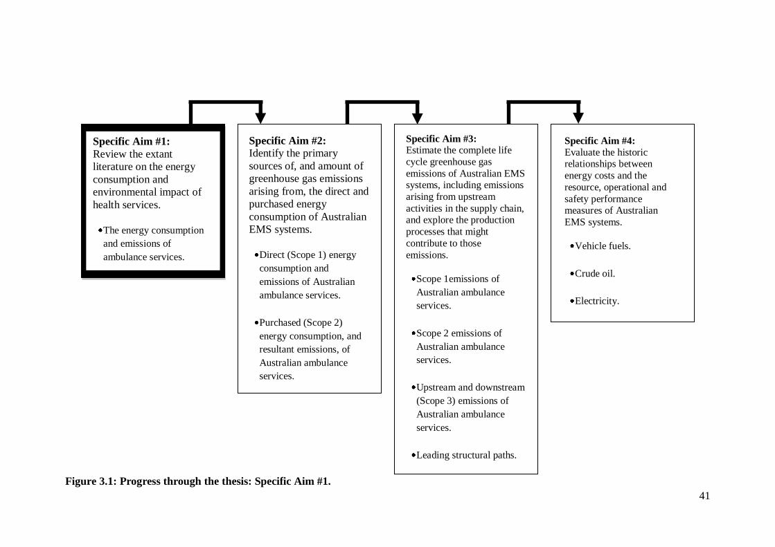
41

Figure 3.1: Progress through the thesis: Specific Aim #1.

Specific Aim #1:

Review the extant

literature on the energy

consumption and

environmental impact of

health services.

The energy consumption

and emissions of

ambulance services.

Specific Aim #3: Estimate the complete life

cycle greenhouse gas

emissions of Australian EMS systems, including emissions

arising from upstream

activities in the supply chain, and explore the production

processes that might

contribute to those

emissions.

Scope 1emissions of

Australian ambulance

services.

Scope 2 emissions of

Australian ambulance

services.

Upstream and downstream

(Scope 3) emissions of

Australian ambulance

services.

Leading structural paths.

Specific Aim #2:

Identify the primary

sources of, and amount of

greenhouse gas emissions

arising from, the direct and

purchased energy

consumption of Australian

EMS systems.

Direct (Scope 1) energy

consumption and

emissions of Australian

ambulance services.

Purchased (Scope 2)

energy consumption, and

resultant emissions, of

Australian ambulance

services.

Specific Aim #4:

Evaluate the historic relationships between

energy costs and the

resource, operational and

safety performance measures of Australian

EMS systems.

Vehicle fuels.

Crude oil.

Electricity.

42

3.1 Abstract

Understanding the energy consumption and environmental impact of health

services is important for both minimising their impact and guiding their adaptation to a

low-carbon economy. This review summarises the English language literature on the

energy burden and environmental impact of health services. All years of the PubMed,

CINAHL and ScienceDirect databases were searched to identify publications reporting

energy consumption, greenhouse gas emissions, and/or the environmental impact of

health-related activities. Data were extracted and tabulated to enable cross-comparisons

among different activities and services; where possible, per-patient or per-event

emissions were calculated. Thirty-two relevant publications were identified. On a per-

patient or per-event basis, energy consumption and greenhouse gas emissions are quite

modest; on an aggregate basis, however, they are substantial. In England and the U.S.,

health-related emissions account for 3% and 8% of total national emissions,

respectively. While reducing health-related energy consumption and greenhouse gas

emissions alone will not solve all of the problems around energy scarcity and climate

change, it can make a meaningful contribution.

3.2 Search Strategies

3.2.1 Searching the Medical Literature

In order to identify published articles reporting or evaluating the energy

consumption of and/or greenhouse gas emissions arising from health services, the

National Library of Medicine (PubMed) database was searched using the Entrez search

engine. The search strategy (Table 3.1) included relevant search terms identified using

the search engine’s medical subject heading (MeSH) thesaurus; it was intended to be as

sensitive, rather than as specific, as possible. The search was first executed 09

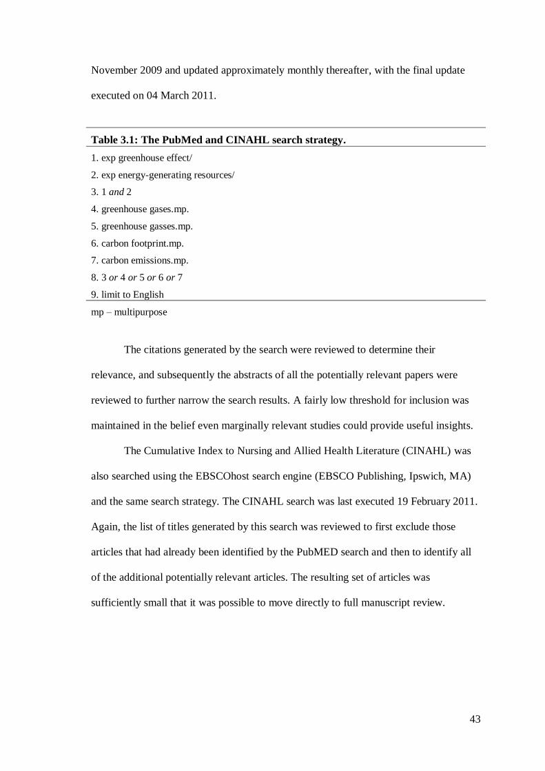
43

November 2009 and updated approximately monthly thereafter, with the final update

executed on 04 March 2011.

The citations generated by the search were reviewed to determine their

relevance, and subsequently the abstracts of all the potentially relevant papers were

reviewed to further narrow the search results. A fairly low threshold for inclusion was

maintained in the belief even marginally relevant studies could provide useful insights.

The Cumulative Index to Nursing and Allied Health Literature (CINAHL) was

also searched using the EBSCOhost search engine (EBSCO Publishing, Ipswich, MA)

and the same search strategy. The CINAHL search was last executed 19 February 2011.

Again, the list of titles generated by this search was reviewed to first exclude those

articles that had already been identified by the PubMED search and then to identify all

of the additional potentially relevant articles. The resulting set of articles was

sufficiently small that it was possible to move directly to full manuscript review.

Table 3.1: The PubMed and CINAHL search strategy.

1. exp greenhouse effect/

2. exp energy-generating resources/

3. 1 and 2

4. greenhouse gases.mp.

5. greenhouse gasses.mp.

6. carbon footprint.mp.

7. carbon emissions.mp.

8. 3 or 4 or 5 or 6 or 7

9. limit to English

mp – multipurpose

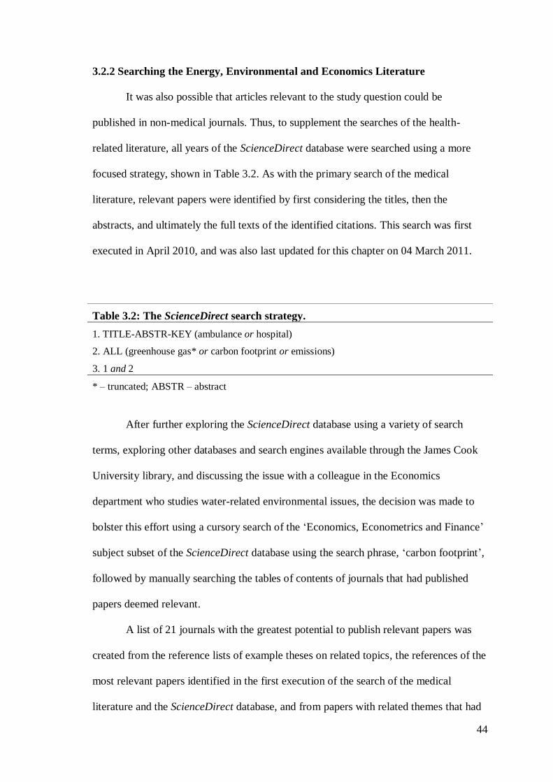
44

3.2.2 Searching the Energy, Environmental and Economics Literature

It was also possible that articles relevant to the study question could be

published in non-medical journals. Thus, to supplement the searches of the health-

related literature, all years of the ScienceDirect database were searched using a more

focused strategy, shown in Table 3.2. As with the primary search of the medical

literature, relevant papers were identified by first considering the titles, then the

abstracts, and ultimately the full texts of the identified citations. This search was first

executed in April 2010, and was also last updated for this chapter on 04 March 2011.

After further exploring the ScienceDirect database using a variety of search

terms, exploring other databases and search engines available through the James Cook

University library, and discussing the issue with a colleague in the Economics

department who studies water-related environmental issues, the decision was made to

bolster this effort using a cursory search of the ‘Economics, Econometrics and Finance’

subject subset of the ScienceDirect database using the search phrase, ‘carbon footprint’,

followed by manually searching the tables of contents of journals that had published

papers deemed relevant.

A list of 21 journals with the greatest potential to publish relevant papers was

created from the reference lists of example theses on related topics, the references of the

most relevant papers identified in the first execution of the search of the medical

literature and the ScienceDirect database, and from papers with related themes that had

Table 3.2: The ScienceDirect search strategy.

1. TITLE-ABSTR-KEY (ambulance or hospital)

2. ALL (greenhouse gas* or carbon footprint or emissions)

3. 1 and 2

* – truncated; ABSTR – abstract

45

been suggested by colleagues. Nine of these journals are indexed in PubMed and thus

relevant articles could be captured by the primary search strategy, but for the remaining

12 journals (Table 3.3) the ScienceDirect database was used to access and manually

review their tables of contents.

This search was first executed in April 2010, including all issues published since

the beginning of the previous year; the search was updated in August 2010, and then

approximately each month thereafter until March 2011. For this search process it was

more efficient to review the titles and abstracts simultaneously, and then download the

full text of any potentially relevant articles. As with the primary search of the medical

literature, a low threshold was maintained for relevance and inclusion.

Table 3.3: Energy and environmental journals subjected to table of contents

search.

Ecological Economics

Energy

Energy Conversion & Management

Energy Economics

Energy Policy

Environmental Impact Assessment Review

Global Environmental Change

Journal of Cleaner Production

Journal of Environmental Economics and Management

Land Use Policy

Renewable Energy

Transportation Research Part D

46

3.2.3 Identifying Additional Papers

Additional relevant papers were identified from the references of the articles

identified by these two search processes, from additional personal reading, and through

referrals of related papers from colleagues.

3.2.4 Categorisation and Classification of Articles

Even within the results of the PubMed and CINAHL searches, the vast majority

of the identified articles were not specifically relevant to energy or emissions

inventories in health or medical settings. This was more true for the results of the

ScienceDirect and table of contents searches, as well as for the additional articles

identified by reviewing cited references. To organise these papers into common themes,

they were sorted into the categories shown in Table 3.4. The primary emphasis was on

identifying articles that reported efforts to measure, characterise or mitigate energy

consumption and emissions in health or medically related settings; the remaining

categories included papers reporting background information on greenhouse gas

emissions and climate change, methodological approaches to inventorying and

modelling energy consumption and greenhouse gas emissions, and examples of energy-

and emissions-related studies from other disciplines that might serve as useful models.

The subset of articles addressing energy consumption and emissions in health

and medical settings was further classified in a method similar to that used in previous

public health related literature surveys (Sanson-Fisher, Campbell, Perkins, Blunden, &

Davis, 2006; Sanson-Fisher, Campbell, Htun, Bailey, & Millar, 2008) as being: original

research; brief reports and research letters; advocacy articles and letters (including those

47

in trade journals); government agency reports; editorials and commentaries; and news

items.

3.2.5 Extraction of Data

For those papers reporting energy consumption and/or emissions data in health

or medical settings—including original research articles, brief reports and research

letters, and government agency reports—data were extracted and tabulated to the extent

possible in order to form a rough understanding of the energy and environmental burden

of health services, and to enable some crude cross-comparisons among different

activities and services. For the emissions data, where possible, per-patient or per-event

emissions were calculated by dividing total reported emissions by the number of

patients or events represented in the data.

3.3 Results

3.3.1 Overall Search Results

As at 04 March 2011 the PubMed search had identified 938 titles for review, the

CINAHL search had identified 66 titles, and the ScienceDirect search had identified 40

titles. From these, 413 were selected for abstract review with 223 retained for evaluation

of the full manuscript; nine of these, however, could not be obtained. The cursory

search of the ScienceDirect ‘Economics, Econometrics and Finance’ subject subset, the

table of contents search (which included review of the contents of 251 journal issues),

and searching the reference lists of the identified papers and related theses identified

more than 600 additional citations (although many were duplicates); from these, 283

articles were obtained for full review. In total, over the course of 16 months nearly 500

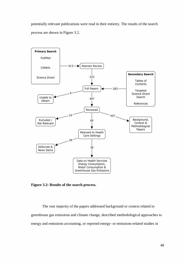
48

potentially relevant publications were read in their entirety. The results of the search

process are shown in Figure 3.2.

Figure 3.2: Results of the search process.

The vast majority of the papers addressed background or context related to

greenhouse gas emissions and climate change, described methodological approaches to

energy and emissions accounting, or reported energy- or emissions-related studies in

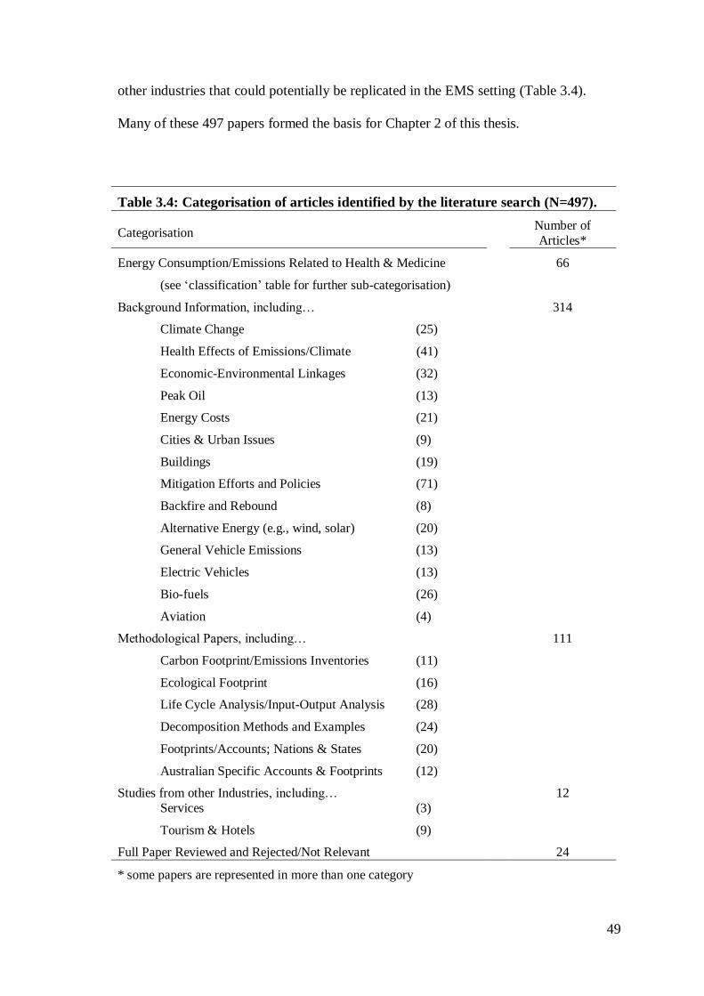
49

other industries that could potentially be replicated in the EMS setting (Table 3.4).

Many of these 497 papers formed the basis for Chapter 2 of this thesis.

Table 3.4: Categorisation of articles identified by the literature search (N=497).

Categorisation Number of

Articles*

Energy Consumption/Emissions Related to Health & Medicine

(see ‘classification’ table for further sub-categorisation)

66

Background Information, including…

Climate Change (25)

Health Effects of Emissions/Climate (41)

Economic-Environmental Linkages (32)

Peak Oil (13)

Energy Costs (21)

Cities & Urban Issues (9)

Buildings (19)

Mitigation Efforts and Policies (71)

Backfire and Rebound (8)

Alternative Energy (e.g., wind, solar) (20)

General Vehicle Emissions (13)

Electric Vehicles (13)

Bio-fuels (26)

Aviation (4)

314

Methodological Papers, including…

Carbon Footprint/Emissions Inventories (11)

Ecological Footprint (16)

Life Cycle Analysis/Input-Output Analysis (28)

Decomposition Methods and Examples (24)

Footprints/Accounts; Nations & States (20)

Australian Specific Accounts & Footprints (12)

111

Studies from other Industries, including…

Services (3)

Tourism & Hotels (9)

12

Full Paper Reviewed and Rejected/Not Relevant 24

* some papers are represented in more than one category

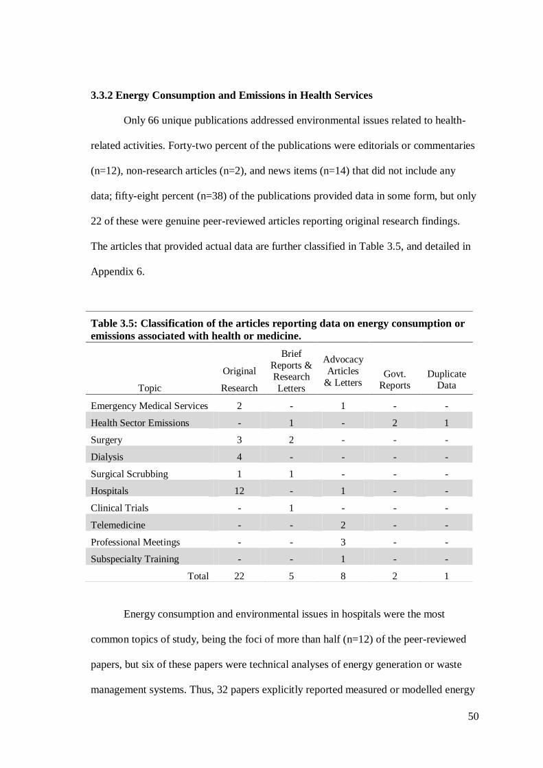
50

3.3.2 Energy Consumption and Emissions in Health Services

Only 66 unique publications addressed environmental issues related to health-

related activities. Forty-two percent of the publications were editorials or commentaries

(n=12), non-research articles (n=2), and news items (n=14) that did not include any

data; fifty-eight percent (n=38) of the publications provided data in some form, but only

22 of these were genuine peer-reviewed articles reporting original research findings.

The articles that provided actual data are further classified in Table 3.5, and detailed in

Appendix 6.

Energy consumption and environmental issues in hospitals were the most

common topics of study, being the foci of more than half (n=12) of the peer-reviewed

papers, but six of these papers were technical analyses of energy generation or waste

management systems. Thus, 32 papers explicitly reported measured or modelled energy

Table 3.5: Classification of the articles reporting data on energy consumption or

emissions associated with health or medicine.

Topic

Original

Research

Brief

Reports & Research

Letters

Advocacy

Articles

& Letters

Govt. Reports

Duplicate Data

Emergency Medical Services 2 - 1 - -

Health Sector Emissions - 1 - 2 1

Surgery 3 2 - - -

Dialysis 4 - - - -

Surgical Scrubbing 1 1 - - -

Hospitals 12 - 1 - -

Clinical Trials - 1 - - -

Telemedicine - - 2 - -

Professional Meetings - - 3 - -

Subspecialty Training - - 1 - -

Total 22 5 8 2 1

51

consumption, greenhouse gas emissions or water consumption in health settings; these

form the core of this review. Twenty-two of these papers reported original data

collection and analysis, either through empirical study or modelling; the remaining ten

papers were advocacy or non-research articles reporting secondary or anecdotal data.

3.3.2(a) Emergency Medical Services

The two peer-reviewed research papers addressing energy consumption of and

emissions from EMS systems identified by the search were papers related to, but not

included as chapters within, this thesis. Having demonstrated the ability of EMS

systems to provide the necessary data in a ‘proof of concept’ study (Blanchard &

Brown, 2009), a colleague and I had undertaken a study to characterise the carbon

emissions from a broad sample of North American EMS agencies (Blanchard & Brown,

2011) (Appendix 5). Fifteen diverse North American EMS systems with over 550,000

combined annual responses and serving a population of 6.3 million reported their direct

and purchased (Scope 1 and Scope 2) energy consumption for one year. Participating

agencies included government ‘third service’ (n=4), public utility model (n=1), private

contractor (n=6) and rural rescue squad (n=4) systems. Their annual call volumes

ranged from 800 to 114,280 (median 20,093; inter-quartile range (IQR) 1,100 – 55,217).

Total CO2e emissions were calculated using Environmental Protection Agency,

Energy Information Administration (EIA) and locality specific emission conversion

factors. Per-response and population-based emissions were also calculated. Emissions

totalled 21,289 t CO2e; 75% of emissions were from diesel or gasoline consumption.

For systems providing complete Scope 1 and Scope 2 data for ground ambulance

operations, emissions averaged 45.5 kg CO2e per response; median emissions per

response were 36.6 (IQR 29.5 – 48.3) kg of CO2e and median emissions per service-

52

area resident were 3.5 (IQR 2.1 – 5.1) kg of CO2e . Two systems reported aviation fuel

consumption for air medical services, with emissions of 1.1 t CO2e per flight, or 0.3 kg

of CO2e per service-area resident. Using population and ambulance response data for

the U.S., this study estimated that annual EMS emissions in that nation total between

660,000 and 1.6 million t CO2e.

In one trade journal article, Hawkins (2008) described the use of a gasoline-

electric hybrid sports utility vehicle as an EMS quick response vehicle (QRV), asserting

that such a vehicle can perform as well as traditional heavy duty QRVs while reducing

both fuel costs and emissions.

3.3.2 (b) Emissions from the Health Sector

The most aggressive attempt to identify and reduce greenhouse gas emissions

associated with health and medical services has been undertaken by England’s National

Health Service’s (NHS) ‘Sustainable Development Unit (SDU)’ in collaboration with

the Stockholm Environment Institute. The SDU was established to monitor

consumption and encourage energy efficient practices in NHS England; its director, Dr.

David Pencheon, has reportedly said that energy use and climate change are essential

issues for the NHS (Creagh, 2008).

Supplementing input-output analysis based on NHS expenditures with more

detailed data on building energy consumption and travel estimates from a National

Travel Survey, the total life cycle carbon footprint of NHS England for calendar year

2004 was estimated at 21.3 million tonnes (Mt) of CO2e, or approximately 3.2% of all

emissions in England (Sustainable Development Commission-Stockholm Environment

Institute, 2008). Eighty-seven percent of those emissions (18.6 Mt) were CO2 emissions,

with the remainder (2.7 Mt) being CO2e emissions of other greenhouse gases. Upstream

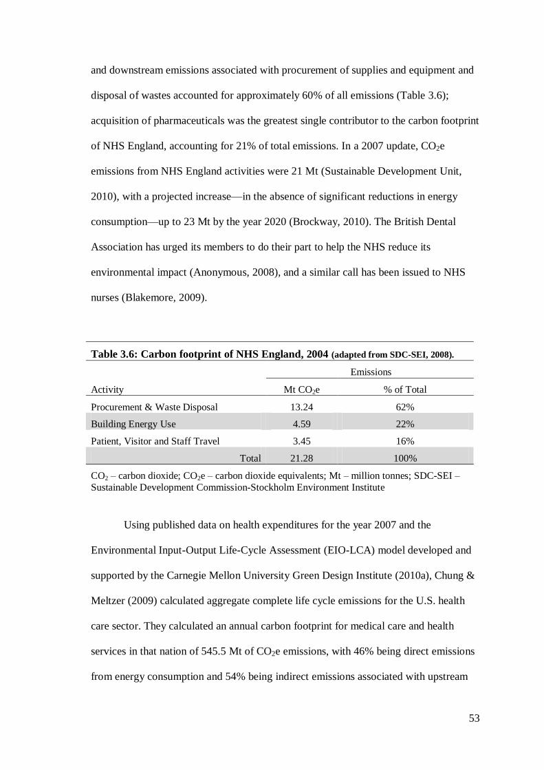
53

and downstream emissions associated with procurement of supplies and equipment and

disposal of wastes accounted for approximately 60% of all emissions (Table 3.6);

acquisition of pharmaceuticals was the greatest single contributor to the carbon footprint

of NHS England, accounting for 21% of total emissions. In a 2007 update, CO2e

emissions from NHS England activities were 21 Mt (Sustainable Development Unit,

2010), with a projected increase—in the absence of significant reductions in energy

consumption—up to 23 Mt by the year 2020 (Brockway, 2010). The British Dental

Association has urged its members to do their part to help the NHS reduce its

environmental impact (Anonymous, 2008), and a similar call has been issued to NHS

nurses (Blakemore, 2009).

Table 3.6: Carbon footprint of NHS England, 2004 (adapted from SDC-SEI, 2008).

Emissions

Activity Mt CO2e % of Total

Procurement & Waste Disposal 13.24 62%

Building Energy Use 4.59 22%

Patient, Visitor and Staff Travel 3.45 16%

Total 21.28 100%

CO2 – carbon dioxide; CO2e – carbon dioxide equivalents; Mt – million tonnes; SDC-SEI –

Sustainable Development Commission-Stockholm Environment Institute

Using published data on health expenditures for the year 2007 and the

Environmental Input-Output Life-Cycle Assessment (EIO-LCA) model developed and

supported by the Carnegie Mellon University Green Design Institute (2010a), Chung &

Meltzer (2009) calculated aggregate complete life cycle emissions for the U.S. health

care sector. They calculated an annual carbon footprint for medical care and health

services in that nation of 545.5 Mt of CO2e emissions, with 46% being direct emissions

from energy consumption and 54% being indirect emissions associated with upstream

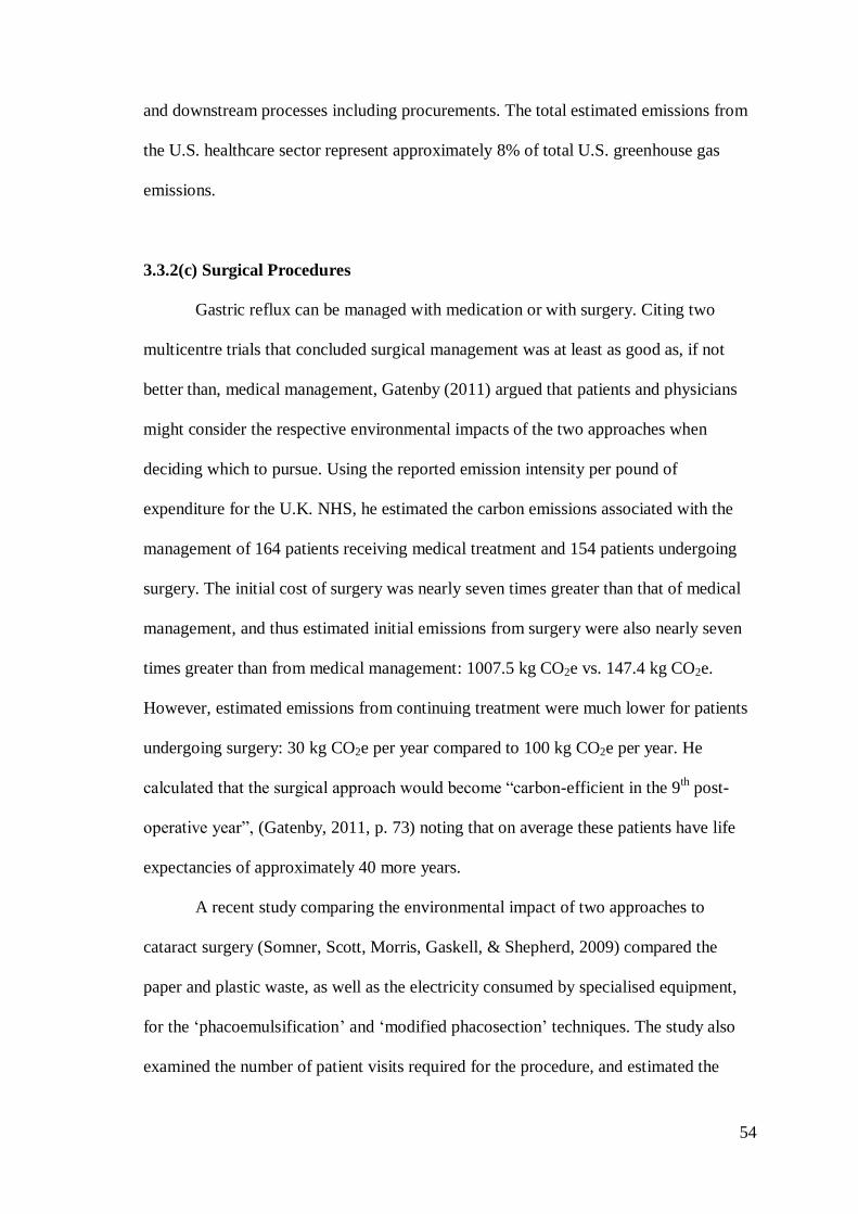
54

and downstream processes including procurements. The total estimated emissions from

the U.S. healthcare sector represent approximately 8% of total U.S. greenhouse gas

emissions.

3.3.2(c) Surgical Procedures

Gastric reflux can be managed with medication or with surgery. Citing two

multicentre trials that concluded surgical management was at least as good as, if not

better than, medical management, Gatenby (2011) argued that patients and physicians

might consider the respective environmental impacts of the two approaches when

deciding which to pursue. Using the reported emission intensity per pound of

expenditure for the U.K. NHS, he estimated the carbon emissions associated with the

management of 164 patients receiving medical treatment and 154 patients undergoing

surgery. The initial cost of surgery was nearly seven times greater than that of medical

management, and thus estimated initial emissions from surgery were also nearly seven

times greater than from medical management: 1007.5 kg CO2e vs. 147.4 kg CO2e.

However, estimated emissions from continuing treatment were much lower for patients

undergoing surgery: 30 kg CO2e per year compared to 100 kg CO2e per year. He

calculated that the surgical approach would become “carbon-efficient in the 9th post-

operative year”, (Gatenby, 2011, p. 73) noting that on average these patients have life

expectancies of approximately 40 more years.

A recent study comparing the environmental impact of two approaches to

cataract surgery (Somner, Scott, Morris, Gaskell, & Shepherd, 2009) compared the

paper and plastic waste, as well as the electricity consumed by specialised equipment,

for the ‘phacoemulsification’ and ‘modified phacosection’ techniques. The study also

examined the number of patient visits required for the procedure, and estimated the

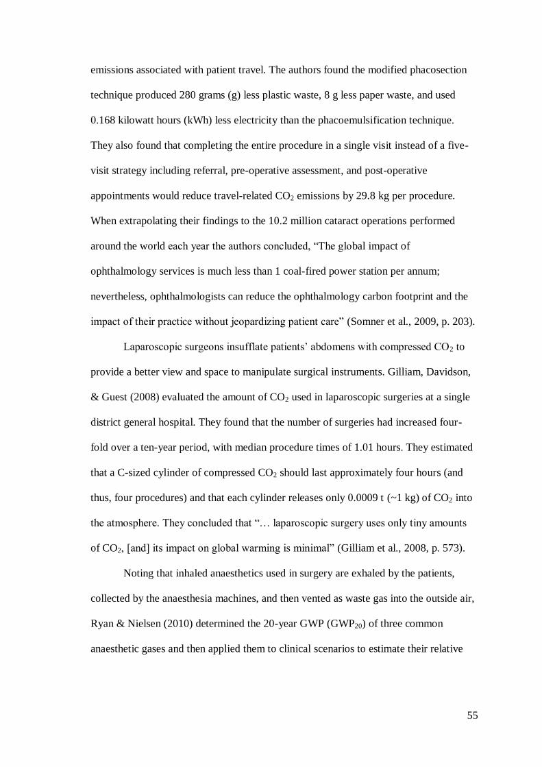
55

emissions associated with patient travel. The authors found the modified phacosection

technique produced 280 grams (g) less plastic waste, 8 g less paper waste, and used

0.168 kilowatt hours (kWh) less electricity than the phacoemulsification technique.

They also found that completing the entire procedure in a single visit instead of a five-

visit strategy including referral, pre-operative assessment, and post-operative

appointments would reduce travel-related CO2 emissions by 29.8 kg per procedure.

When extrapolating their findings to the 10.2 million cataract operations performed

around the world each year the authors concluded, “The global impact of

ophthalmology services is much less than 1 coal-fired power station per annum;

nevertheless, ophthalmologists can reduce the ophthalmology carbon footprint and the

impact of their practice without jeopardizing patient care” (Somner et al., 2009, p. 203).

Laparoscopic surgeons insufflate patients’ abdomens with compressed CO2 to

provide a better view and space to manipulate surgical instruments. Gilliam, Davidson,

& Guest (2008) evaluated the amount of CO2 used in laparoscopic surgeries at a single

district general hospital. They found that the number of surgeries had increased four-

fold over a ten-year period, with median procedure times of 1.01 hours. They estimated

that a C-sized cylinder of compressed CO2 should last approximately four hours (and

thus, four procedures) and that each cylinder releases only 0.0009 t (~1 kg) of CO2 into

the atmosphere. They concluded that “… laparoscopic surgery uses only tiny amounts

of CO2, [and] its impact on global warming is minimal” (Gilliam et al., 2008, p. 573).

Noting that inhaled anaesthetics used in surgery are exhaled by the patients,

collected by the anaesthesia machines, and then vented as waste gas into the outside air,

Ryan & Nielsen (2010) determined the 20-year GWP (GWP20) of three common

anaesthetic gases and then applied them to clinical scenarios to estimate their relative

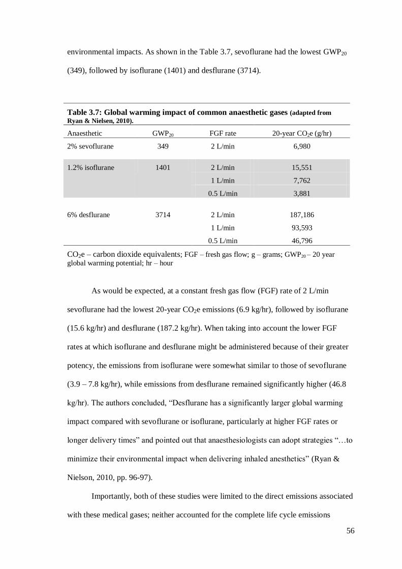
56

environmental impacts. As shown in the Table 3.7, sevoflurane had the lowest GWP20

(349), followed by isoflurane (1401) and desflurane (3714).

Table 3.7: Global warming impact of common anaesthetic gases (adapted from

Ryan & Nielsen, 2010).

Anaesthetic GWP20 FGF rate 20-year CO2e (g/hr)

2% sevoflurane 349 2 L/min 6,980

1.2% isoflurane 1401 2 L/min 15,551

1 L/min 7,762

0.5 L/min 3,881

6% desflurane 3714 2 L/min 187,186

1 L/min 93,593

0.5 L/min 46,796

CO2e – carbon dioxide equivalents; FGF – fresh gas flow; g – grams; GWP20 – 20 year

global warming potential; hr – hour

As would be expected, at a constant fresh gas flow (FGF) rate of 2 L/min

sevoflurane had the lowest 20-year CO2e emissions (6.9 kg/hr), followed by isoflurane

(15.6 kg/hr) and desflurane (187.2 kg/hr). When taking into account the lower FGF

rates at which isoflurane and desflurane might be administered because of their greater

potency, the emissions from isoflurane were somewhat similar to those of sevoflurane

(3.9 – 7.8 kg/hr), while emissions from desflurane remained significantly higher (46.8

kg/hr). The authors concluded, “Desflurane has a significantly larger global warming

impact compared with sevoflurane or isoflurane, particularly at higher FGF rates or

longer delivery times” and pointed out that anaesthesiologists can adopt strategies “…to

minimize their environmental impact when delivering inhaled anesthetics” (Ryan &

Nielson, 2010, pp. 96-97).

Importantly, both of these studies were limited to the direct emissions associated

with these medical gases; neither accounted for the complete life cycle emissions

57

associated with producing, bottling and distributing these gases, which could be

substantial. Although medical gases are not specifically identified, the Carnegie-Melon

based EIO-LCA life cycle assessment tool estimates 4.6 t of CO2e are emitted for every

$1,000 in purchases from U.S. industrial gas manufacturers (Carnegie Mellon

University Green Design Institute, 2010b).

One laboratory study (Bayazit & Sparrow, 2010) has explored the energy

consumption of different perioperative warming devices. Two convective-air warming

devices and two direct-contact conduction warming devices were evaluated using

thermocouples and heat-flux sensors applied to a constant-temperature heat sink serving

as a surrogate patient. Energy efficiency was measured as the ratio of the rate at which

energy was absorbed by the heat sink to the rate at which energy was consumed by the

warming device. The authors found that neither category of device was more efficient

than the other; instead they concluded, “… the appropriate use of insulation and the

suppression of pathways of extraneous heat loss have to be considered in the design of

patient warming devices. It is these factors that created significant differences in the

energy utilisation efficiencies of investigated devices…” (Bayazit & Sparrow, 2010, p.

1214).

3.3.2(d) Water Consumption

Dialysis is a lifesaving treatment for many people with kidney disease, who

often require multiple treatments each week either in a clinic setting or at home.

Dialysis is, however, a water-intense therapy consuming between 120 to 800 litres (L)

of fresh water for each treatment, depending on the type (clinic vs. home) and duration

of the therapy session (Agar, 2010; Agar, Simmonds, Knight, & Somerville, 2009;

Tarrass, Benjelloun, & Benjelloun, 2008). Much of that water is discarded in the reverse

58

osmosis process which creates the dialysis fluid, and it is known as ‘reject water’ (RW).

While officially a medical waste product, RW has been shown to be essentially

bacteria-free, with pH, turbidity and electrolyte characteristics not unlike those of

municipal and industrial water supplies (Agar, 2010; Agar et al., 2009; Tarras et al.,

2008). As such, recycling of RW for use as gray water—for example, irrigating lawns

or flushing toilets—has been advocated and even trialled in some settings (Agar, 2010).

The cost of recycling RW is estimated to be less than that of generating fresh water

through reverse osmosis of sea water (Tarrass et al., 2008). This practice, however, is

not widespread. For example, only two of 58 renal units in England, Scotland and

Wales that participated in a survey on ‘sustainability in kidney care’ reported having

RW recycling facilities; indeed, nearly two-thirds of the participating centres didn’t

even have water-saving taps for their sinks (Connor & Mortimer, 2010).

The ‘sustainability in kidney care’ survey also provided additional insights into

the energy conservation efforts of U.K. dialysis centres. Only 30% of the responding

centres used low-energy light bulbs in all or most of their light fixtures; only two

centres used solar energy to supplement their electricity consumption and none used

wind turbines; in 61% of the facilities the staff could not adjust the heating or air

conditioning (which arguably could be either an energy saver or an energy waster).

More positively, more than 80% of the responding centres actively encouraged staff to

bicycle to work and provided cycle parking and shower facilities to support that, and

25% recaptured heat from the dialysis effluent to offset some of their energy burden

(Connor & Mortimer, 2010).

Somner et al. (2008) evaluated two types of water taps for surgical scrub sinks to

determine whether “environmentally friendly scrubbing behaviour [would lead] to less

energy and water expenditure per scrub” (Somner et al., 2008, p 213). They observed

59

scrubbing at two Scottish hospitals, one where the tap was turned on using the elbow

and one where the tap was turned on with the leg, recording the length of time for which

the tap was running using a stopwatch. Six doctors and eight nurses scrubbed a total of

25 times. Where the tap was activated by the elbow, the tap was on for a mean of 2

minutes and 23 seconds per scrub; where the tap was activated by the leg, the tap was

on for a mean of 1 minute and 7 seconds. This translated to a difference of 5.7 L of

water per scrub, and the authors estimated that changing all U.K. surgical sinks from

elbow-activated to leg-activated taps would save approximately 11,000 gigajoules (GJ)

(or 3,000,000 kWh) annually in energy required to heat the water. They concluded, “…

if we are all to play a part in reducing our impact on the environment, simple

interventions like this can combine to make a major impact on climate change and its

prevention” (Somner et al., 2008, p. 214).

Jones (2009) conducted a similar study, collecting water from the drains of three

different types of scrub bays—one with an elbow-controlled tap, one with a spring-

loaded foot-controlled tap, and one with a motion-sensor-controlled tap—used in a

standardised five-minute scrub routine. He found that when the water flow was turned

off between rinses, the volume of water consumed was similar across the three types of

taps (6.7 to 7.5 L), but only the spring-loaded foot controlled tap turned off

automatically between rinses. When motion-sensor-controlled and elbow-controlled

taps ran continuously they consumed three times as much water (20.2 and 24.9 L,

respectively), and if the elbow-controlled tap was left continuously opened at a high

flow rate the amount of water consumed exceeded 50 L per scrub. He concluded,

“Surgical scrub staff can have a significant role in reducing the use of potable water

supplies. … It could also be reduced at an organisational level by either retrofitting

older facilities or, when building new ones, by selecting the most water-sparing

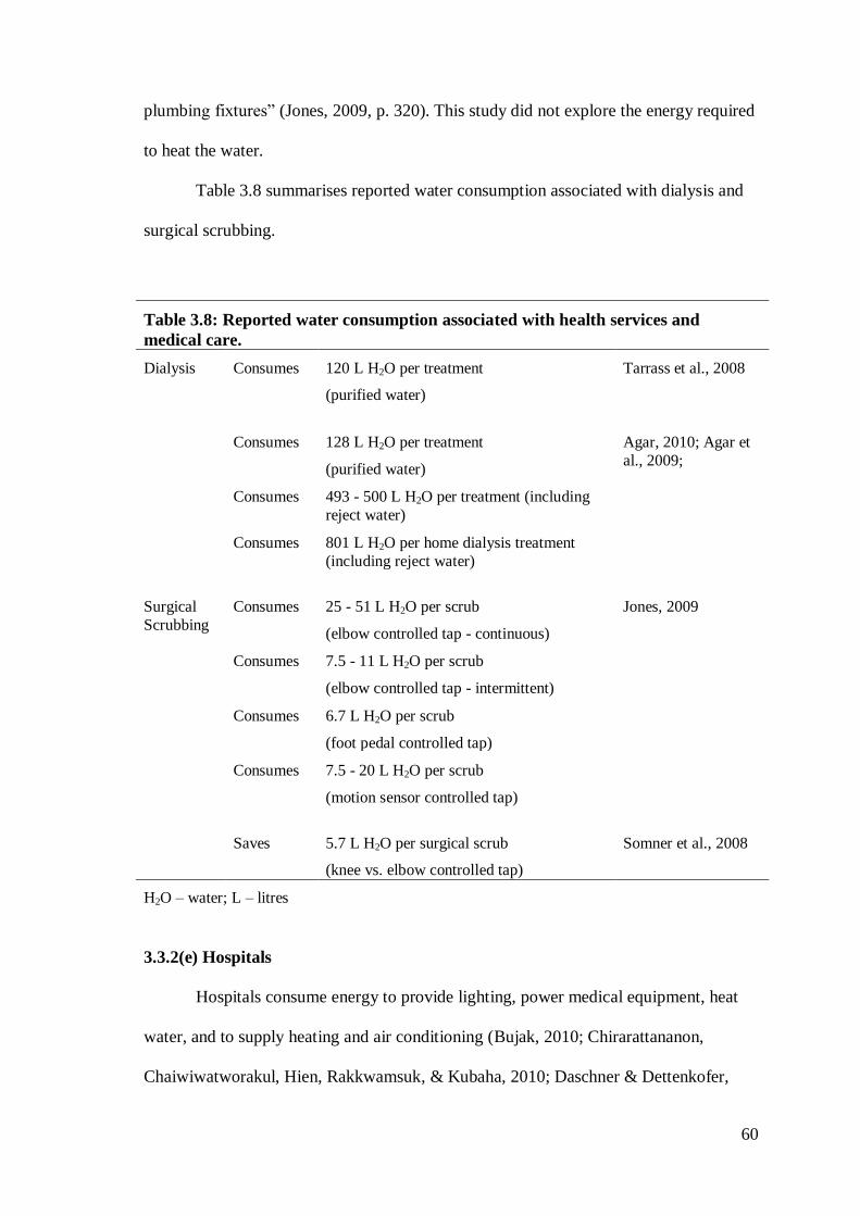
60

plumbing fixtures” (Jones, 2009, p. 320). This study did not explore the energy required

to heat the water.

Table 3.8 summarises reported water consumption associated with dialysis and

surgical scrubbing.

Table 3.8: Reported water consumption associated with health services and

medical care.

Dialysis Consumes 120 L H2O per treatment

(purified water)

Tarrass et al., 2008

Consumes 128 L H2O per treatment

(purified water)

Agar, 2010; Agar et

al., 2009;

Consumes 493 - 500 L H2O per treatment (including

reject water)

Consumes 801 L H2O per home dialysis treatment

(including reject water)

Surgical

Scrubbing

Consumes 25 - 51 L H2O per scrub

(elbow controlled tap - continuous)

Jones, 2009

Consumes 7.5 - 11 L H2O per scrub

(elbow controlled tap - intermittent)

Consumes 6.7 L H2O per scrub

(foot pedal controlled tap)

Consumes 7.5 - 20 L H2O per scrub

(motion sensor controlled tap)

Saves 5.7 L H2O per surgical scrub

(knee vs. elbow controlled tap)

Somner et al., 2008

H2O – water; L – litres

3.3.2(e) Hospitals

Hospitals consume energy to provide lighting, power medical equipment, heat

water, and to supply heating and air conditioning (Bujak, 2010; Chirarattananon,

Chaiwiwatworakul, Hien, Rakkwamsuk, & Kubaha, 2010; Daschner & Dettenkofer,

61

1997; Gaglia et al., 2007; Renedo, Ortiz, Manana, Silio, & Perez, 2006; Saidur,

Hasanuzzaman, Yogeswaran, Mohammed, & Hossain, 2010). They also produce waste,

both in terms of single-use disposable supplies and waste water (Daschner &

Dettenkofer, 1997; Karagiannidis, Papageorgiou, Perkoulidis, Sanida, & Samaras,

2010). Finally, there are indirect energy and environmental impacts associated with

their purchasing activities (Daschner & Dettenkofer, 1997).

Compared to other non-residential buildings, hospitals consume more energy per

square metre (m2) of floor space due in part to their continuous, 24-hour operations

(Gaglia et al., 2007). The reported annual thermal and electrical energy consumption per

m2 of floor space—or ‘energy intensity’—of hospitals, clinics and other health facilities

is remarkably consistent over both geography and time, ranging roughly between 230

kWh/m2 to 330 kWh/m

2 (Table 3.9) (Bujak, 2010; Chirarattananon, Chaiwiwatworakul,

Hien, Rakkwamsuk, & Kubaha, 2010; Gaglia et al., 2007; Murray, Pahl, & Burek,

2008; Saidur, Hasanuzzaman, Yogeswaran, Mohammed, & Hossain, 2010) with the

exception of a single hospital in Spain (Renedo, Ortiz, Manana, Silio, & Perez, 2006).

Murray et al. (2008) estimated that for small health facilities in Scotland, this translates

into 86 kg/m2 of CO2 emissions, but the greenhouse gas emissions of the facilities

represented in the other studies could vary substantially from this, depending on their

energy mix (electricity, natural gas, etc) and the primary fuel source used by their

electricity supplier (coal, hydro, nuclear, etc).

Heating domestic hot water is a particularly noteworthy energy sink for

hospitals, accounting for approximately 20% of the energy burden of two Polish

hospitals (Bujak, 2010). Thus, the potential water savings from modifying the taps in

surgical scrub sinks as described by Somner et al. (2008) and Jones (2009) could also

translate into energy savings. Another possible mechanism for reducing energy

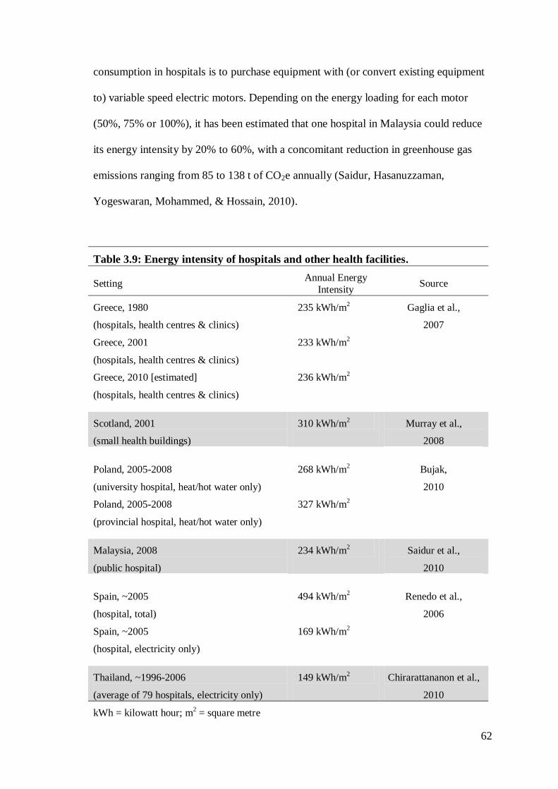
62

consumption in hospitals is to purchase equipment with (or convert existing equipment

to) variable speed electric motors. Depending on the energy loading for each motor

(50%, 75% or 100%), it has been estimated that one hospital in Malaysia could reduce

its energy intensity by 20% to 60%, with a concomitant reduction in greenhouse gas

emissions ranging from 85 to 138 t of CO2e annually (Saidur, Hasanuzzaman,

Yogeswaran, Mohammed, & Hossain, 2010).

Table 3.9: Energy intensity of hospitals and other health facilities.

Setting Annual Energy

Intensity Source

Greece, 1980

(hospitals, health centres & clinics)

235 kWh/m2

Gaglia et al.,

2007

Greece, 2001

(hospitals, health centres & clinics)

233 kWh/m2

Greece, 2010 [estimated]

(hospitals, health centres & clinics)

236 kWh/m2

Scotland, 2001

(small health buildings)

310 kWh/m2

Murray et al.,

2008

Poland, 2005-2008

(university hospital, heat/hot water only)

268 kWh/m2

Bujak,

2010

Poland, 2005-2008

(provincial hospital, heat/hot water only)

327 kWh/m2

Malaysia, 2008

(public hospital)

234 kWh/m2

Saidur et al.,

2010

Spain, ~2005

(hospital, total)

494 kWh/m2

Renedo et al.,

2006

Spain, ~2005

(hospital, electricity only)

169 kWh/m2

Thailand, ~1996-2006

(average of 79 hospitals, electricity only)

149 kWh/m2

Chirarattananon et al.,

2010

kWh = kilowatt hour; m2 = square metre

63

New hospitals and health facilities can also reduce their energy consumption

through design measures that accentuate natural ventilation and reduce the need for air

conditioning (Lomas & Ji, 2009), and through compliance with modern building energy

codes (Chirarattananon, Chaiwiwatworakul, Hien, Rakkwamsuk, & Kubaha, 2010).

Hospitals can also supplement their energy needs with on-site power generation,

which can both produce cost savings (Bizzarri & Morini, 2004; Lozano, Ramos,

Carvalho, & Serra, 2009; Renedo, Ortiz, Manana, Silio, & Perez, 2006) and reduce

greenhouse gas emissions (Bizzarri & Morini, 2004; 2006). Fuel cells that convert

chemical energy into electricity (Bizzarri & Morini, 2004; 2006; Damberger, 1998),

solar collectors that use fluid-filled piping to capture the sun’s heat (Bizzari & Morini

2006; Tsoutsos, Aloumpi, Gkouskos, & Karagiorgas, 2010), and photovoltaic solar

collectors that directly convert solar energy to electricity (Bizzari & Morini, 2006) have

all been advocated as on-site power generation technologies that hospitals can use to

reduce their consumption of commercial energy and lower their greenhouse gas

emissions. The payback time on the initial investment, however, currently makes these

strategies economically non-viable: the most optimistic estimate is 11.5 years (Tsoutsos

et al., 2010) with most estimates ranging between 20 and 30 years (Bizzari & Morini,

2004; 2006), which far exceeds the usable life of the proposed systems.

3.3.2(f) Ancillary Health System Activities

Research: In 2007, under the moniker ‘The Sustainable Trials Study Group’,

Burnett et al. (2007) evaluated the emissions associated with the Corticosteroid

Randomisation after Significant Head Injury (CRASH) Trial evaluating the effect of

corticosteroid administration on outcomes of adults with head injury. Based at the

64

London School of Hygiene and Tropical Medicine, the five-year trial recruited 10,008

subjects from 49 nations. Using the protocol recommended by the World Business

Council for Sustainable Development, the investigators estimated emissions associated

with fuel use, refrigerant loss and electricity consumption at the trial coordinating

centre, fuel use for deliveries and travel, and waste disposal for one year of the trial.

Emissions totalled 126 t of CO2e; the investigators extrapolated emissions for the full

five year trial to be 630 t of CO2e, or approximately 63 kg of CO2e per study subject.

The coordination centre was responsible for 39% of the emissions, with nearly all of its

emissions arising from electricity consumption. Distribution of study medications and

documents was responsible for 28% of the emissions, and study-related travel

accounted for 23%. Trial team commuting and shipping of study drugs from the

producer to the coordinating centre were responsible for the remaining 10% of

emissions. The investigators concluded, “Clinical trials are energy intensive and

produce substantial greenhouse gas emissions” (Burnett et al., 2007, p. 672). They

further recommended that the “…research community must ensure that trials look at

questions of greatest priority using methods compatible with broader strategic

objectives in relation to environment and health” and “… establish awareness about the

broader consequences of health care and research…” (Burnett et al., 2007, pp. 672-673).

More recently, the CRASH investigators reported they were able to substantially reduce

study-related emissions in the CRASH-2 trial, primarily through increased efficiency in

subject recruitment (Subaiya, Hogg, & Roberts, 2011).

Telemedicine: Telemedicine is the practice of using internet-based audio-visual

links to provide patient consultations to sites where physicians, specialist physicians,

and/or other health professionals are not available. In a letter to the British Medical

Journal, Smith, Patterson, & Scott (2007) described three examples of telemedicine—

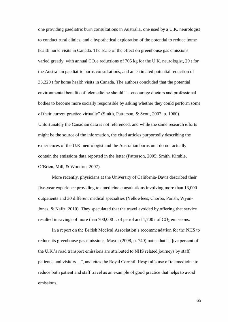
65

one providing paediatric burn consultations in Australia, one used by a U.K. neurologist

to conduct rural clinics, and a hypothetical exploration of the potential to reduce home

health nurse visits in Canada. The scale of the effect on greenhouse gas emissions

varied greatly, with annual CO2e reductions of 705 kg for the U.K. neurologist, 29 t for

the Australian paediatric burns consultations, and an estimated potential reduction of

33,220 t for home health visits in Canada. The authors concluded that the potential

environmental benefits of telemedicine should “…encourage doctors and professional

bodies to become more socially responsible by asking whether they could perform some

of their current practice virtually” (Smith, Patterson, & Scott, 2007, p. 1060).

Unfortunately the Canadian data is not referenced, and while the same research efforts

might be the source of the information, the cited articles purportedly describing the

experiences of the U.K. neurologist and the Australian burns unit do not actually

contain the emissions data reported in the letter (Patterson, 2005; Smith, Kimble,

O’Brien, Mill, & Wootton, 2007).

More recently, physicians at the University of California-Davis described their

five-year experience providing telemedicine consultations involving more than 13,000

outpatients and 30 different medical specialties (Yellowlees, Chorba, Parish, Wynn-

Jones, & Nafiz, 2010). They speculated that the travel avoided by offering that service

resulted in savings of more than 700,000 L of petrol and 1,700 t of CO2 emissions.

In a report on the British Medical Association’s recommendation for the NHS to

reduce its greenhouse gas emissions, Mayor (2008, p. 740) notes that “[f]ive percent of

the U.K.’s road transport emissions are attributed to NHS related journeys by staff,

patients, and visitors…”, and cites the Royal Cornhill Hospital’s use of telemedicine to

reduce both patient and staff travel as an example of good practice that helps to avoid

emissions.

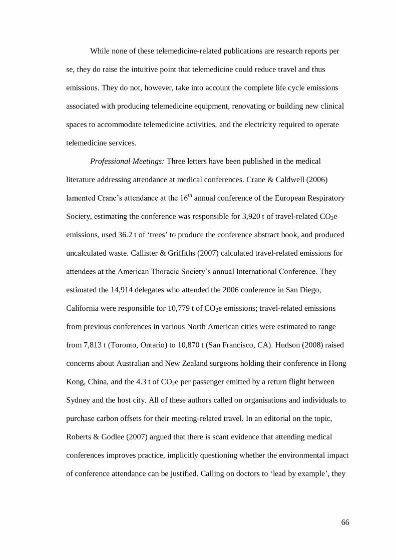
66

While none of these telemedicine-related publications are research reports per

se, they do raise the intuitive point that telemedicine could reduce travel and thus

emissions. They do not, however, take into account the complete life cycle emissions

associated with producing telemedicine equipment, renovating or building new clinical

spaces to accommodate telemedicine activities, and the electricity required to operate

telemedicine services.

Professional Meetings: Three letters have been published in the medical

literature addressing attendance at medical conferences. Crane & Caldwell (2006)

lamented Crane’s attendance at the 16th annual conference of the European Respiratory

Society, estimating the conference was responsible for 3,920 t of travel-related CO2e

emissions, used 36.2 t of ‘trees’ to produce the conference abstract book, and produced

uncalculated waste. Callister & Griffiths (2007) calculated travel-related emissions for

attendees at the American Thoracic Society’s annual International Conference. They

estimated the 14,914 delegates who attended the 2006 conference in San Diego,

California were responsible for 10,779 t of CO2e emissions; travel-related emissions

from previous conferences in various North American cities were estimated to range

from 7,813 t (Toronto, Ontario) to 10,870 t (San Francisco, CA). Hudson (2008) raised

concerns about Australian and New Zealand surgeons holding their conference in Hong

Kong, China, and the 4.3 t of CO2e per passenger emitted by a return flight between

Sydney and the host city. All of these authors called on organisations and individuals to

purchase carbon offsets for their meeting-related travel. In an editorial on the topic,

Roberts & Godlee (2007) argued that there is scant evidence that attending medical

conferences improves practice, implicitly questioning whether the environmental impact

of conference attendance can be justified. Calling on doctors to ‘lead by example’, they

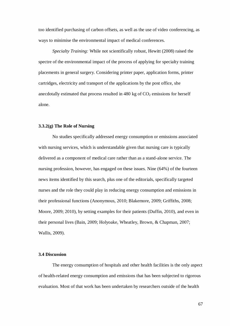
67

too identified purchasing of carbon offsets, as well as the use of video conferencing, as

ways to minimise the environmental impact of medical conferences.

Specialty Training: While not scientifically robust, Hewitt (2008) raised the

spectre of the environmental impact of the process of applying for specialty training

placements in general surgery. Considering printer paper, application forms, printer

cartridges, electricity and transport of the applications by the post office, she

anecdotally estimated that process resulted in 480 kg of CO2 emissions for herself

alone.

3.3.2(g) The Role of Nursing

No studies specifically addressed energy consumption or emissions associated

with nursing services, which is understandable given that nursing care is typically

delivered as a component of medical care rather than as a stand-alone service. The

nursing profession, however, has engaged on these issues. Nine (64%) of the fourteen

news items identified by this search, plus one of the editorials, specifically targeted

nurses and the role they could play in reducing energy consumption and emissions in

their professional functions (Anonymous, 2010; Blakemore, 2009; Griffiths, 2008;

Moore, 2009; 2010), by setting examples for their patients (Duffin, 2010), and even in

their personal lives (Bain, 2009; Holyoake, Wheatley, Brown, & Chapman, 2007;

Wallis, 2009).

3.4 Discussion

The energy consumption of hospitals and other health facilities is the only aspect

of health-related energy consumption and emissions that has been subjected to rigorous

evaluation. Most of that work has been undertaken by researchers outside of the health

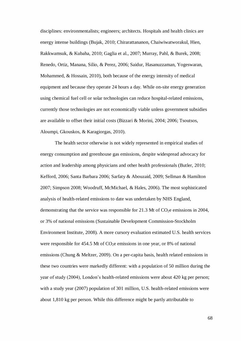
68

disciplines: environmentalists; engineers; architects. Hospitals and health clinics are

energy intense buildings (Bujak, 2010; Chirarattananon, Chaiwiwatworakul, Hien,

Rakkwamsuk, & Kubaha, 2010; Gaglia et al., 2007; Murray, Pahl, & Burek, 2008;

Renedo, Ortiz, Manana, Silio, & Perez, 2006; Saidur, Hasanuzzaman, Yogeswaran,

Mohammed, & Hossain, 2010), both because of the energy intensity of medical

equipment and because they operate 24 hours a day. While on-site energy generation

using chemical fuel cell or solar technologies can reduce hospital-related emissions,

currently those technologies are not economically viable unless government subsidies

are available to offset their initial costs (Bizzari & Morini, 2004; 2006; Tsoutsos,

Aloumpi, Gkouskos, & Karagiorgas, 2010).

The health sector otherwise is not widely represented in empirical studies of

energy consumption and greenhouse gas emissions, despite widespread advocacy for

action and leadership among physicians and other health professionals (Butler, 2010;

Kefford, 2006; Santa Barbara 2006; Sarfaty & Abouzaid, 2009; Sellman & Hamilton

2007; Simpson 2008; Woodruff, McMichael, & Hales, 2006). The most sophisticated

analysis of health-related emissions to date was undertaken by NHS England,

demonstrating that the service was responsible for 21.3 Mt of CO2e emissions in 2004,

or 3% of national emissions (Sustainable Development Commission-Stockholm

Environment Institute, 2008). A more cursory evaluation estimated U.S. health services

were responsible for 454.5 Mt of CO2e emissions in one year, or 8% of national

emissions (Chung & Meltzer, 2009). On a per-capita basis, health related emissions in

these two countries were markedly different: with a population of 50 million during the

year of study (2004), London’s health-related emissions were about 420 kg per person;

with a study year (2007) population of 301 million, U.S. health-related emissions were

about 1,810 kg per person. While this difference might be partly attributable to

69

differences in the structure of health services in these two countries, some (but not all)

of the difference might also be an artefact of using input-output analysis and emissions

per unit of expenditure to calculate their respective carbon footprints. Per-capita health

expenditures in the U.S. are roughly 240% higher than in the U.K. (Organisation for

Economic Co-operation and Development, 2010).

The reported emissions from health-related activities are summarised in Table

3.10. The current evidence is almost entirely based on small narrowly focused studies,

and to some extent on methodologically weak or anecdotal reports. Still, the data do

indicate that per-patient or per-treatment emissions are relatively modest. Even when

extrapolating these emissions to national or global patient visits, are health related

emissions significant enough to warrant attention? These numbers pale in comparison to

global emissions: 49 billion t of CO2e in 2004 (Intergovernmental Panel on Climate

Change, 2007).

Indeed, national greenhouse gas inventories typically only identify the four IPPC

‘Annex A’ economic sectors required under the Kyoto Protocol: Energy Generation

(fuel combustion and fugitive emissions); Industrial Processes; Waste; and Agriculture

(Australian Government Department of Climate Change, 2009b)—and notably not

health care. However, emissions from health services are comparable to those of other

important economic sectors. In the U.S., for example, emissions from the ‘Agriculture’

sector total approximately 500 million metric tons of CO2e annually, representing

around 7% of total national emissions (U.S. Environmental Protection Agency, 2011).

The ‘Waste Management’ sector is responsible for approximately 3% of total emissions

in the U.K. (Department of Energy and Climate Change, 2011).

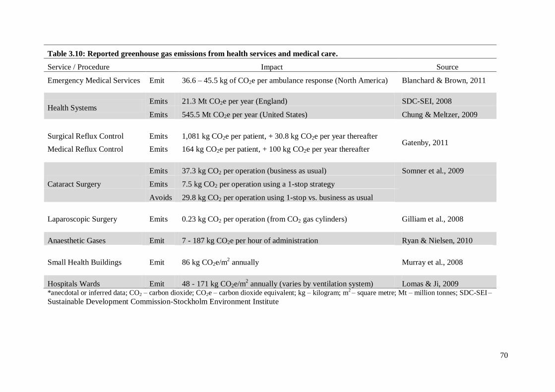
70

*anecdotal or inferred data; CO2 – carbon dioxide; CO2e – carbon dioxide equivalent; kg – kilogram; m2 – square metre; Mt – million tonnes; SDC-SEI

–

Sustainable Development Commission-Stockholm Environment Institute

Table 3.10: Reported greenhouse gas emissions from health services and medical care.

Service / Procedure Impact Source

Emergency Medical Services Emit 36.6 – 45.5 kg of CO2e per ambulance response (North America) Blanchard & Brown, 2011

Health Systems Emits 21.3 Mt CO2e per year (England) SDC-SEI, 2008

Emits 545.5 Mt CO2e per year (United States) Chung & Meltzer, 2009

Surgical Reflux Control Emits 1,081 kg CO2e per patient, + 30.8 kg CO2e per year thereafter Gatenby, 2011

Medical Reflux Control Emits 164 kg CO2e per patient, + 100 kg CO2e per year thereafter

Cataract Surgery

Emits 37.3 kg CO2 per operation (business as usual) Somner et al., 2009

Emits 7.5 kg CO2 per operation using a 1-stop strategy

Avoids 29.8 kg CO2 per operation using 1-stop vs. business as usual

Laparoscopic Surgery Emits 0.23 kg CO2 per operation (from CO2 gas cylinders) Gilliam et al., 2008

Anaesthetic Gases Emit 7 - 187 kg CO2e per hour of administration Ryan & Nielsen, 2010

Small Health Buildings Emit 86 kg CO2e/m2 annually Murray et al., 2008

Hospitals Wards Emit 48 - 171 kg CO2e/m2 annually (varies by ventilation system) Lomas & Ji, 2009

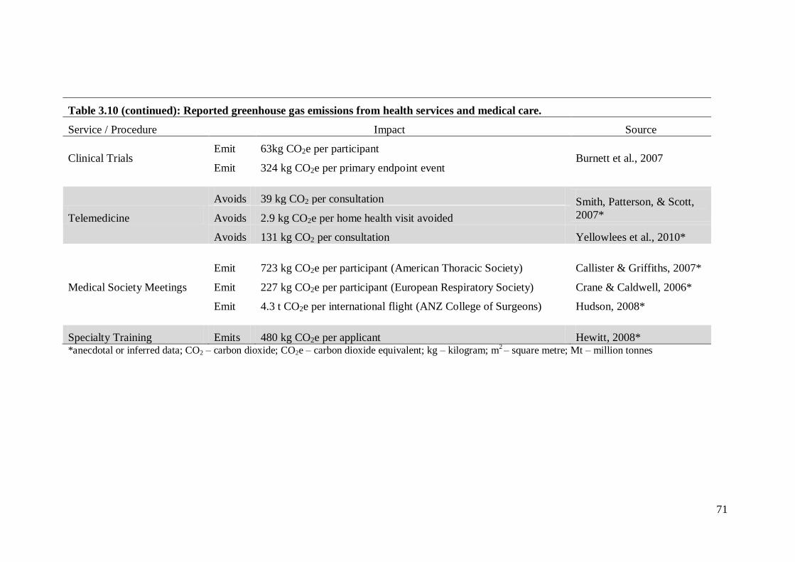
71

Table 3.10 (continued): Reported greenhouse gas emissions from health services and medical care.

Service / Procedure Impact Source

Clinical Trials Emit 63kg CO2e per participant

Burnett et al., 2007 Emit 324 kg CO2e per primary endpoint event

Telemedicine

Avoids 39 kg CO2 per consultation Smith, Patterson, & Scott,

2007* Avoids 2.9 kg CO2e per home health visit avoided

Avoids 131 kg CO2 per consultation Yellowlees et al., 2010*

Medical Society Meetings

Emit 723 kg CO2e per participant (American Thoracic Society) Callister & Griffiths, 2007*

Emit 227 kg CO2e per participant (European Respiratory Society) Crane & Caldwell, 2006*

Emit 4.3 t CO2e per international flight (ANZ College of Surgeons) Hudson, 2008*

Specialty Training Emits 480 kg CO2e per applicant Hewitt, 2008* *anecdotal or inferred data; CO2 – carbon dioxide; CO2e – carbon dioxide equivalent; kg – kilogram; m

2 – square metre; Mt – million tonnes

72

The juxtaposition of total Australian national emissions with U.S. health care

sector emissions is also instructive when considering this point. In 2007 and 2008,

Australia’s greenhouse gas emissions totalled 547 Mt and 553 Mt of CO2e,

respectively (Australian Government Department of Climate Change, 2009b). That is,

U.S. health sector emissions are of the same scale as Australia’s total national

emission. While reducing health-related emissions alone will not solve all of the

problems around GHGs and climate change, it can make a meaningful contribution: a

10% reduction in emissions from just the U.S. health system would have the same

atmospheric impact as a 10% reduction in emissions from the entire Australian

economy. Numerous authors have described how reducing atmospheric CO2 levels

and mitigating climate change will only succeed through the cumulative energy and

emissions savings of many such incremental policy initiatives and efforts (e.g.:

Coontz, 2007; Lenzen & Smith, 1999/2000; McCollum & Yang, 2009; Mulugetta,

Jackson, & van der Horst, 2010; Pacala & Socolow, 2004; Reynolds, 2010; Scholes,

2009).

Some health systems are already taking steps to minimize their environmental

impact, most notably the systematic efforts of NHS England (Brockway, 2010). A

recent survey of 14 directors of primary care trusts in southwest England found that

seven were pursuing sustainability strategies, including the sourcing of green energy,

green travel policies such as supporting cycling to work, procurement policies

designed to minimize packaging and waste, and the sourcing of local food products

for cafeterias (Nichols & Richardson, 2011). Other logical steps that health systems

could take to reduce their energy consumption and greenhouse gas consumption

include, for example, incorporating natural ventilation and green building concepts

when constructing or renovating health facilities (Bizzarri & Morini, 2006;

73

Chirarattananon, Chaiwiwatworakul, Hien, Rakkwamsuk, & Kubaha, 2010; Lomas &

Ji, 2009) or including more hybrid vehicles in the corporate fleet (Hawkins, 2008).

Lastly, health systems and health professionals should not underestimate their

potential influence on broader sustainability efforts; their stature within the

community makes them ideal advocates and role models.

A more practical and perhaps more immediate concern is how mounting

energy scarcity, increasing energy costs, and societal pressures to reduce emissions

might actually pose a threat to the delivery of health services. Thus, understanding the

energy consumption and emissions associated with health services is important not

only to identify opportunities to minimise the environmental impact of those services,

but also to identify the energy and emissions-related threats to those services in order

to better guide their adaptation to a low-carbon economy. Managing greenhouse gas

emissions is managing energy consumption, and vice-versa. It is a ‘win-win’

proposition.

3.5 Summary of Health Service Energy Consumption and Emissions

The health sector is not well represented in the energy- and emissions-related

literature. The only report a of sector-wide effort to inventory health-related

greenhouse gas emissions comes from NHS England, where health services were

estimated to produce 21.3 Mt of CO2e in 2004, or 3% of national emissions for that

year (Sustainable Development Commission-Stockholm Environment Institute, 2008).

In the U.S., health services are estimated to be responsible for 454.5 Mt of CO2e

emissions each year, or 8% of national emissions (Chung & Meltzer, 2009).

The only reports of energy consumption and emissions from EMS systems are

those from the North American studies related to, but not included as part of, this

74

thesis. There, ambulance services are estimated to produce between 36.6 and 45.5 kg

CO2e of Scope 1 and Scope 2 greenhouse gas emissions per ambulance response. The

next chapter begins the process of determining the environmental burden of

ambulance services in Australia by inventorying their Scope 1 and Scope 2 energy

consumption, and calculating the resultant greenhouse gas emissions.

75

Chapter 4: The Carbon Footprint of Australian Ambulance Operations

Chapter 2 laid out the theoretical and methodological framework for this

thesis, and Chapter 3 reviewed the extant literature on health-related energy

consumption and greenhouse gas emissions. This chapter describes the effort to

determine the Scope 1 and Scope 2 emissions of Australian ambulance systems

(Figure 4.1).

This chapter has been adapted into a manuscript: Brown L.H., Canyon, D.V.,

Buettner, P.G., Crawford, J.M., Judd, J, on behalf of the Australian Ambulance

Emissions Study Group. (In Press). The carbon footprint of Australian ambulance

operations. Emergency Medicine Australasia. Accepted 15 May 2012. Documentation

of acceptance is included in Appendix 2.

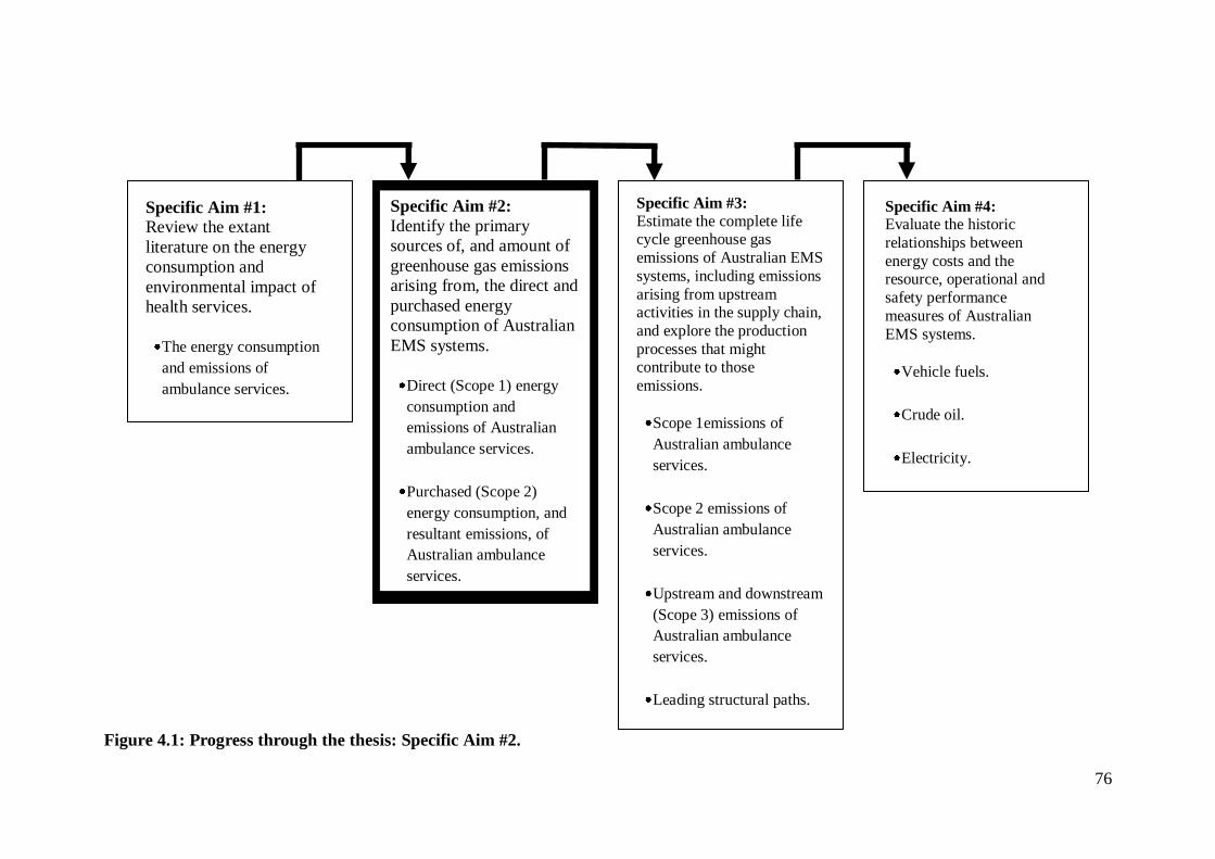
76

Figure 4.1: Progress through the thesis: Specific Aim #2.

Specific Aim #1:

Review the extant

literature on the energy

consumption and

environmental impact of

health services.

The energy consumption

and emissions of

ambulance services.

Specific Aim #3:

Estimate the complete life cycle greenhouse gas

emissions of Australian EMS

systems, including emissions

arising from upstream activities in the supply chain,

and explore the production

processes that might contribute to those

emissions.

Scope 1emissions of

Australian ambulance

services.

Scope 2 emissions of

Australian ambulance

services.

Upstream and downstream

(Scope 3) emissions of

Australian ambulance

services.

Leading structural paths.

Specific Aim #2:

Identify the primary

sources of, and amount of

greenhouse gas emissions

arising from, the direct and

purchased energy

consumption of Australian

EMS systems.

Direct (Scope 1) energy

consumption and

emissions of Australian

ambulance services.

Purchased (Scope 2)

energy consumption, and

resultant emissions, of

Australian ambulance

services.

Specific Aim #4: Evaluate the historic

relationships between

energy costs and the resource, operational and

safety performance

measures of Australian

EMS systems.

Vehicle fuels.

Crude oil.

Electricity.

77

4.1 Abstract

The objective of this study is to determine the greenhouse gas emissions

associated with the direct and purchased energy consumption of Australian ambulance

operations, and to identify the predominant energy sources that contribute to those

emissions. This two-phase study uses operational and financial data from a convenience

sample of Australian ambulance operations to inventory their energy consumption and

greenhouse gas emissions for one year. State- and territory-based ambulance systems

serving 58% of Australia’s population and performing 59% of Australia’s ambulance

responses provided data for the study. Emissions for the participating systems total

67,390 t of CO2e for the study period, or 35 kg CO2e per ambulance response, 48 kg

CO2e per patient transport, and 5 kg CO2e per capita. Vehicle fuels account for 58% of

the emissions from ground ambulance operations, with the remainder primarily

attributable to electricity consumption. Emissions from air ambulance transport are

nearly 200 times those for ground ambulance transport. On a national level, emissions

from Australian ambulance operations are estimated to be between 110,000 and 120,000

t of CO2e each year.

4.2 Introduction

The literature review in Chapter 3 established that the greenhouse gas emissions

from individual medical procedures or health services are modest, but in the aggregate

they are substantial. Health sector emissions account for 3% of all greenhouse gas

emissions in the U.K. (Sustainable Development Commission-Stockholm Environment

Institute, 2008), and 8% of greenhouse gas emissions in the U.S. (Chung & Meltzer,

2009). The contribution of individual health-related services to Australian national

greenhouse gas emissions has not been empirically studied. To characterise the

78

emissions associated with ambulance operations in Australia, this study addressed two

questions: (1) What are the Scope 1 and Scope 2 greenhouse gas emissions associated

with Australian ambulance operations? and (2) What energy sources are the primary

contributors to the Scope 1 and Scope 2 greenhouse gas emissions of Australian

ambulance operations?

4.3 Methods

4.3.1 Design, Setting and Participants

This study evaluates data from the operational and financial records of a

convenience sample of Australian ambulance operations. The study was conducted in

two phases: a pilot phase evaluating test-retest consistency of the data collection

process, and a final phase with full data collection and analysis.

As described in Chapter 2, greenhouse gas emission inventories are typically

classified by their ‘scope’. Scope 1 emissions are those that arise from direct energy

consumption, for example the burning of petrol in vehicles or natural gas in furnaces.

Scope 2 emissions are those that arise from purchased energy consumption, primarily

relating to electricity consumption but also including emissions from travel on

commercial carriers. Scope 3 emissions are those that arise from a product or service’s

upstream and downstream production and waste disposal processes. Finally, ‘complete

life cycle emissions’ represent the sum of Scope 1, Scope 2 and Scope 3 emissions

(Australian Government Department of Climate Change, 2009a). This study explored

the Scope 1 and Scope 2 emissions of Australian ambulance operations.

In Australia, responsibility for ambulance services rests with each state or

territory government; ambulance services are provided by agencies within the

department of health (New South Wales (NSW); South Australia (SA); Tasmania

79

(TAS); Victoria (VIC)) or the department responsible for emergency services

(Australian Capital Territory (ACT); Queensland (QLD)), or through a contract with St.

John’s Ambulance Service—an independent not-for-profit organisation (Northern

Territory (NT); Western Australia (WA)). In the 2009-2010 fiscal year, Australian

ambulance services performed more than 3.5 million emergency and non-emergency

responses (Council of Ambulance Authorities, 2010). The ambulance systems of four

Australian states or territories participated in this study: Ambulance Service New South

Wales (NSW); St. John Ambulance - Northern Territory (NT); SA Ambulance Service

(SA); and Ambulance-Victoria (VIC). Three of the systems participated in the pilot

phase and three systems provided data for the final phase; two systems participated in

both phases. Collectively, the three systems providing data for the final phase of the

study served 58% of Australia’s population and performed 59% of Australia’s

ambulance responses during the study period (Council of Ambulance Authorities,

2010).

4.3.2 Pilot Phase Protocol

For the pilot trial, a data collection tool was developed based on the

methodology used in the North American study of ambulance-related emissions

(Blanchard & Brown, 2011) and with input from the representatives of the participating

Australian ambulance systems. The pilot trial data collection tool asked participants to

report their agency’s energy consumption for a 90-day period during 2009, including:

diesel and petrol for ambulances and other vehicles; on-site energy consumption such as

natural gas and electricity usage at stations and offices; aviation fuel use; and employee

work-related commercial air travel (e.g., travel to conferences and meetings). After a

45-day wash-out period, the respondents were asked to provide the same data for the

80

same period; the importance of re-collecting the data anew, rather than resubmitting the

original data, was emphasised to all participants.

For the pilot trial, an a priori decision was made that a less than 10% difference

in reported ‘test’ and ‘retest’ energy consumption would indicate acceptable test-retest

consistency for the data collection tool. In fact, the ‘test’ and ‘retest’ data were nearly

identical, except that a small amount of compressed natural gas (CNG) consumption

(197 L) reported in the ‘test’ data was reported as liquefied petroleum (LP) consumption

in the ‘retest’ data, and there was an error in pro-rata apportionment of natural gas and

electricity consumption in one system where some facilities were shared with other

agencies. To address this problem, a pro-rating worksheet was developed and

distributed with the data collection tool for the final phase of the study.

4.3.3 Final Phase Protocol

The final version of the data collection tool and pro-rating worksheet are

included as Appendix 7. For the final phase of the study, participants were asked to

report their agency’s energy consumption for a full 12-month period: the most recent

calendar year or financial year for which complete data were available. Participants

were also asked to report their agency’s call volume for the same period, including total

number of responses, number of emergency responses, and number of patients

transported. The population served by each agency was obtained from the Australian

Bureau of Statistics (2011).

4.3.4 Data Analysis

All data were converted into standard units: L for liquid fuels, GJ for natural

gas, and kWh for electricity. For each reported energy source, emissions of CO2e per

81

unit of consumption were calculated using Australian government ‘National

Greenhouse Accounts’ emission factors (Australian Government Department of Climate

Change, 2009c). Aggregate emissions for the participating agencies, as well as

emissions per response, per patient transport, and per capita (that is, per person residing

in the agencies’ respective service areas), are reported. The contributions of individual

energy sources to the total emissions, and the differentiation of emissions from ground

and air ambulance activities, are also reported.

4.4 Ethical Review

The Human Research Ethics Committee (HREC) at James Cook University

approved this study (HREC #H3592, Appendix 1) with the understanding that all data

would be reported in the aggregate. The study was also approved by the research

committee, research director, or managing director of each participating agency.

4.5 Results

The emissions from the reported energy consumption for the three ambulance

systems participating in the final phase of the study totalled 67,390 t of CO2e. This

translates into 35 kg CO2e per ambulance response, 48 kg CO2e per patient transport,

and 5 kg CO2e per capita. Diesel and petrol consumption were responsible for 35% of

the emissions; electricity consumption was responsible for 26% of the emissions; and

aviation fuel consumption was responsible for 38% of the emissions. Other fuel sources

accounted for less than 1% of total emissions (Figure 4.2).

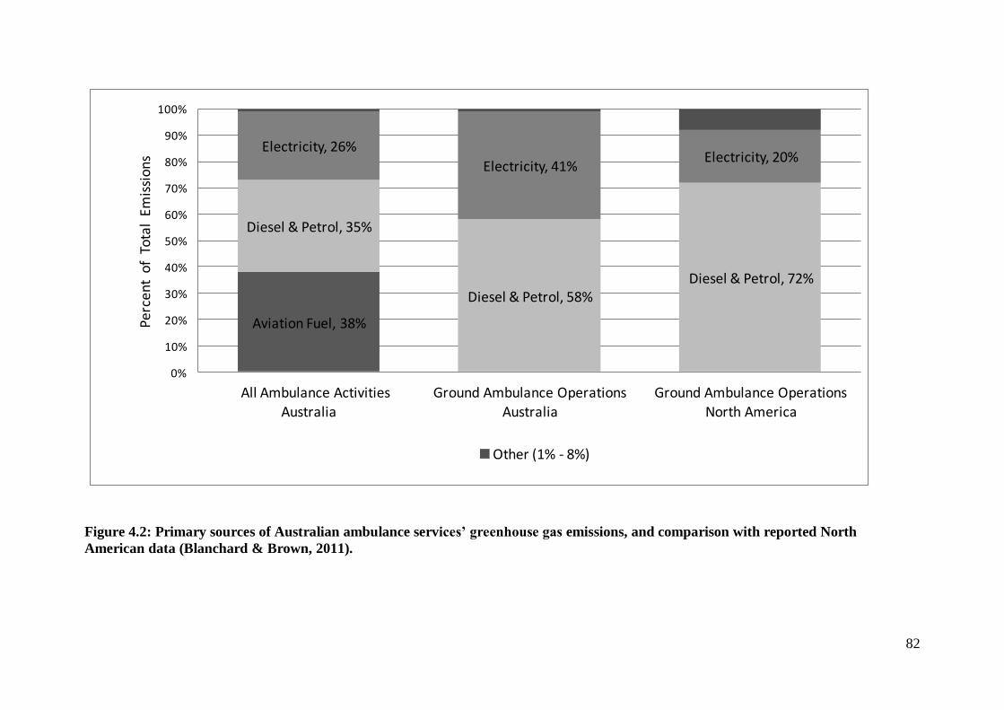
82

Aviation Fuel, 38%

Diesel & Petrol, 35%

Diesel & Petrol, 58%Diesel & Petrol, 72%

Electricity, 26%

Electricity, 41%Electricity, 20%

0%

10%

20%

30%

40%

50%

60%

70%

80%

90%

100%

All Ambulance Activities

Australia

Ground Ambulance Operations

Australia

Ground Ambulance Operations

North America

Per

cen

t o

f T

ota

l Em

issi

on

s

Other (1% - 8%)

Figure 4.2: Primary sources of Australian ambulance services’ greenhouse gas emissions, and comparison with reported North

American data (Blanchard & Brown, 2011).

83

Only two of the participating systems provided air ambulance services and, in

both systems, air ambulance missions represented less than 1% of all patient transports.

When eliminating aviation fuel consumption and air ambulance missions from the

analysis, ground ambulance operations in the three participating systems generated

41,885 t of CO2e emissions for the study period. This equates to 22 kg CO2e per ground

ambulance response, 30 kg CO2e per patient transport, and 3 kg CO2e per capita. Diesel

and petrol consumption were responsible for 58% of the emissions from ground

ambulance activities, with electricity consumption responsible for 41% of the emissions

(Figure 4.2). Emissions from aviation fuel for the two systems providing air ambulance

services totalled 25,505 t of CO2e, or 5.3 t CO2e per air ambulance mission and 5.8 t

CO2e per patient transport.

4.6 Discussion

Consistent with other research on health service emissions, per-patient

greenhouse gas emissions from Australian ground ambulance operations are small.

However, extrapolating these results to the entire nation (5 kg per capita × 22 million

population; 35 kg per response × 3.5 million ambulance responses) suggests aggregate

Scope 1 and Scope 2 emissions from Australian state- and territory-based ground and

air ambulance operations total approximately 110,000 to 120,000 t of CO2e each year.

As Australia’s national emissions approach 550 to 560 Mt annually (Australian

Government Department of Climate Change, 2009b), Scope 1 and Scope 2 emissions

from ambulance operations represent 0.02% of the country’s total greenhouse gas

emissions. This might seem like a small proportion, but the Australian economy is

divided into 19 divisions, 53 subdivisions, 214 industry groups, and finally 506 industry

classes—including ambulance services (Australian Bureau of Statistics, 2006). The

84

estimated Scope 1 emissions from ambulance services (81,000 to 89,000 t CO2e) are

comparable to the direct greenhouse gas emissions from the ‘brown coal’ (93,000 t) or

‘silver and zinc’ (89,000 t) mining sectors reported in a 2005 analysis of the Australian

economy (Foran, Lenzen, & Dey, 2005).

Encouragingly, the average per-response emissions for Australian ground

ambulance operations are half those reported for North American ambulance systems

(22 kg vs. 45 kg CO2e) and the contribution of vehicle fuels to the carbon footprint of

Australian ambulance systems is not as great as for North American systems, 58% vs.

72% (Figure 4.2) (Blanchard & Brown, 2011). This might reflect differences in the

geographical distributions of the populations on the two continents: While Australia is

less densely populated than the U.S. (2.9 people / km2 vs. 33.7 people / km

2), only 12%

of the Australian population live outside of urban areas, compared with 21% of the U.S.

population (Australian Bureau of Statistics, 2011; U.S. Census Bureau, 2011). It could

be a function of the efficiency of the vehicle fleet; light weight van-chassis ambulances

are more common in Australia, while heavier truck-chassis ambulances are more

common in North America. There might also be increased efficiencies associated with

the centralisation of Australian ambulance operations as state or territory governmental

services. In all likelihood, it is some combination of these and other factors.

Despite these favourable comparisons, Australian ambulance operations should

still strive to minimise their environmental impact. Potential strategies for reducing

ambulance system energy consumption and greenhouse gas emissions include reducing

unnecessary ambulance responses and ambulance transports, developing flexible

response time policies, reducing driving speeds when transporting stable patients

without life-threatening conditions, reduced ambulance idling at emergency scenes and

receiving hospitals, the use of hybrid vehicles for administrative and support vehicle

85

fleets, or the use of bio-diesel for ambulances. None of these proposed strategies,

however, have been empirically evaluated; their actual impact on energy consumption

and emissions, as well as patient outcomes, remains to be determined. For example,

while the benefits seem intuitive, bio-diesel is not universally carbon neutral

(Searchinger et al., 2008; Solomon, 2010).

Restricting the use of air ambulances, whether rotor-wing or fixed-wing, to only

those situations in which they are demonstrated to provide some clinical benefit might

also be an intuitive strategy for substantially reducing ambulance system energy

consumption and emissions. In this study, average emissions for air ambulance transport

were nearly 200 times the average emissions for ground ambulance transport, and

emissions for Australian air ambulance missions were approximately five times those of

North American air ambulance missions (Blanchard & Brown, 2011). Yet, reducing air

ambulance responses and transports in Australia could be a particularly difficult task.

Independent of patient clinical condition, many Australian air ambulance missions

involve patients in rural or remote locations where access and transport by ground

ambulance is simply not feasible, and sometimes not possible.

Finally health promotion initiatives, as well as injury and illness prevention

programs, could have a dual effect of improving public health and reducing the demand

for ambulance services, and thus ambulance-related emissions.

4.7 Limitations

This study is limited by its focus on only Scope 1 and Scope 2 greenhouse gas

emissions. While the Scope 3 emissions of Australian ambulance operations were not

explored in this analysis, they would certainly add to the total carbon footprint. In the

U.S. and U.K., Scope 3 emissions represent 54% and 60% of total health sector

86

emissions, respectively (Sustainable Development Commission-Stockholm

Environment Institute, 2008; Chung & Meltzer, 2009). Like other aspects of the health

sector, ambulance services could additionally reduce their total life cycle greenhouse

gas emissions by adopting environmentally conscious purchasing strategies.

This study is also limited by its inclusion of data for only three Australian

ambulance systems, but the participating systems are geographically and climatically

diverse and account for nearly 60% of all ambulance responses in Australia (Council of

Ambulance Authorities, 2010). It is also likely that the energy consumption data

reported by these three systems slightly under-estimate their true Scope 1 and 2 carbon

footprint. Only one system reported employee-related travel, and another system could

not access electricity consumption data for approximately 10% of its facilities, as those

facilities were shared with—and the electricity billing was in the name of—non-

participating third parties. One of the participating systems does not provide ambulance

services for people or events more than 150 km from an ambulance station, thus data for

that small portion of ambulance responses in that geopolitical setting were not included

in this analysis. Still, the participating systems were able to report the vast majority of

their energy consumption. The data should be adequately representative of the national

experience.

Lastly, the comparisons with the emissions from North American ambulance

operations are based on published data from that continent (Blanchard & Brown, 2011),

and were not a specific aim of this study. The methodologies of the two studies,

however, were nearly identical and the comparisons are sound.

87

4.8 Conclusion

In summary, per-response emissions from Australian ground ambulance

operations are substantially lower than those from North American ambulance

operations. Vehicle fuels account for nearly 60% of the emissions from ground

ambulance operations, with the remainder primarily attributable to electricity

consumption. Emissions from air ambulance transport are nearly 200 times those of

ground ambulance transport. Overall, the Scope 1 and Scope 2 energy consumption of

Australian state- and territory-based ground and air ambulance operations produces

approximately 110,000 to 120,000 t of CO2e each year, which is of the same order as

other important sectors of the Australian economy.

What, though, are the complete life cycle emissions of Australian ambulance

services? The next chapter addresses that question.

4.9 Acknowledgements

Contributing members of the Australian Ambulance Services Emissions Study Group:

Simone L. Darke, Ambulance Victoria, Doncaster, VIC

Rob Elliott, SA Ambulance Service, Eastwood, SA

Paul M. Middleton, Ambulance Service of New South Wales, Rozelle, NSW

Peter J. Monks, St. John Ambulance – Northern Territory, Casuarina, NT

Robyne Stewart, Ambulance Service of New South Wales, Rozelle, NSW

88

Chapter 5: The Complete Life Cycle Emissions of Australian Ambulance Services

The previous chapter focused on the Scope 1 and Scope 2 energy consumption

and greenhouse gas emissions of Australian EMS systems. Those are the obvious and

intuitive issues for EMS agencies, but the upstream energy consumption and emissions

associated with the products and services in the ambulance system supply chain should

not be ignored. In this chapter, the complete life cycle emissions of Australian EMS

systems are explored (Figure 5.1).

This chapter has been adapted into a manuscript: Brown, L.H., Canyon, D.V.,

Buettner, P.G., Crawford, J.M., Judd, J. (Under Review). Estimating the complete life

cycle emissions of Australian ambulance operations.

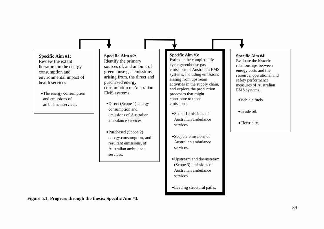
89

Figure 5.1: Progress through the thesis: Specific Aim #3.

Specific Aim #1:

Review the extant

literature on the energy

consumption and

environmental impact of

health services.

The energy consumption

and emissions of

ambulance services.

Specific Aim #3:

Estimate the complete life

cycle greenhouse gas emissions of Australian EMS

systems, including emissions

arising from upstream

activities in the supply chain, and explore the production

processes that might

contribute to those emissions.

Scope 1emissions of

Australian ambulance

services.

Scope 2 emissions of

Australian ambulance

services.

Upstream and downstream

(Scope 3) emissions of

Australian ambulance

services.

Leading structural paths.

Specific Aim #2:

Identify the primary

sources of, and amount of

greenhouse gas emissions

arising from, the direct and

purchased energy

consumption of Australian

EMS systems.

Direct (Scope 1) energy

consumption and

emissions of Australian

ambulance services.

Purchased (Scope 2)

energy consumption, and

resultant emissions, of

Australian ambulance

services.

Specific Aim #4:

Evaluate the historic relationships between

energy costs and the

resource, operational and safety performance

measures of Australian

EMS systems.

Vehicle fuels.

Crude oil.

Electricity.

90

5.1 Abstract

Reducing global greenhouse gas emissions will ultimately depend on multiple

strategies implemented on international, national, local and institutional or

organisational scales. Ambulance services are a vehicle-intense subsector of the health

sector that could contribute to that sector’s emissions reduction efforts. This analysis

uses data from the previous inventory of ambulance service Scope 1 and Scope 2

emissions (Chapter 4), along with publicly available expenditure data and input-output

based multipliers, to estimate the complete life cycle emissions of Australian ambulance

services. Total emissions are estimated at between 216,000 and 547,000 t CO2e

annually, with approximately 20% arising from direct consumption of vehicle and

aircraft fuels, 22% arising from electricity consumption, and 58% arising from upstream

Scope 3 processes. The estimates and the leading structural paths differ substantially

depending on the extent to which inventory-based versus input-output-based data are

incorporated into the estimates, and whether ambulance services’ economic structures

are presumed to resemble those of broader health sector activities, other emergency

services, or general government services. Emissions from ambulance services represent

between 1.8% and 4.4% of total Australian health sector emissions, suggesting that

ambulance services might indeed play a role in that sector’s emissions reduction efforts.

5.2 Introduction

Much of the international emphasis on reducing greenhouse gas emissions has

placed responsibility on national governments (Cushman & Jones, 2002; Macintosh,

2010). In reality, however, a country’s total emissions are the sum of the emissions from

many thousands of relatively low-emitting institutions, firms, and organisations, as well

as thousands, millions or—in the case of India and China—billions of individuals.

91

While national governments might be able to influence the behaviour of organisations,

firms and individuals through policy efforts such as green energy initiatives or carbon

taxes, reducing global greenhouse gas emissions will ultimately depend on the

cumulative successes of multiple strategies implemented on international, national,

local, institutional, organisational and individual scales (Cushman & Jones, 2002;

Mulugetta, Jackson, & van der Horst, 2010; Pacala & Socolow, 2004; Reynolds, 2010).

Healthcare is one example of an economic sector with substantial total

greenhouse gas emissions arising from the aggregation of many low-emitting activities

(see Chapter 3). As with global emissions, for the health sector to substantially reduce

its total greenhouse gas emissions will require the cumulative efforts of hundreds of

component sub-sectors each reducing their emissions on what might appear to be

relatively small scales.

Ambulance services are a vehicle-intense subsector of healthcare that might be

able to disproportionately contribute to the sector’s emissions reduction efforts. In

North America, each ambulance response is estimated to produce 36.6 kg (median) to

45.5 kg (mean) CO2e of Scope 1 and Scope 2 emissions arising from vehicle fuel and

electricity consumption (Blanchard & Brown, 2011). In Australia, ground ambulance

services emit approximately 22 kg CO2e of Scope 1 and Scope 2 emissions per

ambulance response (See Chapter 4). To date, no attempt to characterise the Scope 3

and complete life cycle emissions of ambulance services has been reported.

This study attempts to estimate the complete life cycle emissions associated with

Australian ambulance services through a hybrid assessment incorporating both

inventory-based and input-output based emissions estimates. In addition to quantifying

the contributions of Scope 1, Scope 2 and Scope 3 emissions in the carbon footprint of

Australian ambulance agencies, this study explores the leading structural paths that

92

ambulance services might target in efforts to reduce their greenhouse gas emissions.

Finally, this study exemplifies the difficulties associated with using aggregate sectoral

input-output based multipliers for estimating emissions from diverse sub-sectoral or

cross-sectoral activities.

5.3 Methodology

5.3.1 Data Sources

5.3.1(a) Inventory of Scope 1 and Scope 2 Emissions

Chapter 4 inventoried the Scope 1 and Scope 2 energy consumption and

greenhouse gas emissions of Australian ambulance services, duplicating a methodology

previously used in a similar assessment of North American EMS agencies (Blanchard &

Brown, 2011). To briefly review, three Australian state- or territory-based ambulance

systems, serving 58% of the Australian population and performing 59% of all

Australian ambulance responses, reported their vehicle fuel, aviation fuel, natural gas

and electricity consumption for a 12-month period in 2009-2010. Emission factors from

the Australian government’s ‘National Greenhouse Accounts’ (Australian Government

Department of Climate Change, 2009c) were then used to calculate the CO2e emissions

associated with that energy consumption. From these data, the Scope 1 and Scope 2

emissions from all Australian ground and air ambulance operations were estimated to

total approximately 110,000 to 120,000 t of CO2e each year, with electricity

consumption representing 26% of that total. For this study, the mid-point of that

estimate (115,000 t CO2e) is used as a notional inventory-based estimate of annual

Australian ambulance service Scope 1 and Scope 2 emissions, with 85,100 t CO2e

(74%) arising from direct energy consumption and 29,900 t CO2e (26%) arising from

electricity consumption.

93

5.3.1(b) Input-Output based Multipliers and Structural Path Analyses

Input-output analysis and structural path analysis are both well known and

widely described in the ecological- and energy-economics literature. Input-output

analysis “… is a top-down macroeconomic technique using sectoral monetary

transactions … to account for the complex interdependencies of industries in modern

economies” (Lenzen, 2003, p. 3). Leontief (1970) demonstrated that input-output

analysis could be used to analyse pollutants (as opposed to monetary transactions) as

integral components of economic processes, and since then the technique has been used

in numerous studies to determine the resource flows and environmental impacts

associated with the final consumption of economic sectors (Wiedmann, Minx, Barrett,

& Wackernagel, 2006). Structural path analysis, or decomposition analysis, is the

process of ‘unravelling’ the flows and transactions represented in input-output analyses

in order to identify the principal production chains contributing to the final consumption

within, and the environmental impacts of, an economic sector (Lenzen, 2002; 2003).

Structural paths can be described as ‘zero order’, resulting from transactions within an

individual economic sector, ‘first order’, resulting from the direct transactions between

one economic sector and another, or ‘second (and more distal) order’ resulting from

successive transactions between three (or more) sectors in the production chain.

In 2005, researchers from Australia’s Commonwealth Scientific and Industrial

Research Organisation (CSIRO) and the University of Sydney published a

comprehensive ‘triple bottom line’ (TBL) analysis of the Australian Economy (Foran,

Lenzen, & Dey, 2005). Titled ‘Balancing Act’, this analysis used Australia’s 1994-1995

economy-wide input-output tables to develop a TBL accounting for three financial,

three social and four environmental indicators for all 135 sectors of the Australian

94

economy. Included in this analysis are TBL multipliers showing the relationship

between each of the indicators and gross national expenditure (GNE) or gross national

turnover (GNT) within each sector. One of the included multipliers is greenhouse gas

emissions in kg CO2e per dollar of expenditure; this multiplier is further differentiated

into a multiplier for direct emissions and a multiplier for total emissions. The

‘Balancing Act’ analysis also identifies the leading structural paths contributing to the

greenhouse gas emissions of each economic sector, including their first-order electricity

consumption and the proportion of total emissions attributable to that electricity

consumption.

Ambulance services in Australia are formally classified as a component of the

‘health services’ economic sector (Foran, Lenzen, & Dey, 2005), but they are delivered

by state and territory governments as public goods and they are not universally situated

within Departments of Health; in four Australian states and territories ambulance

services are either delivered by the departments responsible for other emergency

services or function as independent statutory authorities. However they are

administratively structured, the operational characteristics of ambulance systems are

less like those of, for example, hospitals and more like those of other emergency

services such as police departments and fire departments. In Australia, police

departments and fire departments are formally classified as components of the ‘other

services’ economic sector. Due to this cross-sectoral nature of ambulance services, this

analysis incorporates the TBL multipliers and structural paths reported for the ‘health

services’ (Hs), ‘government services’ (Gv) and ‘other services’ (Os) sectors of the

Australian economy.

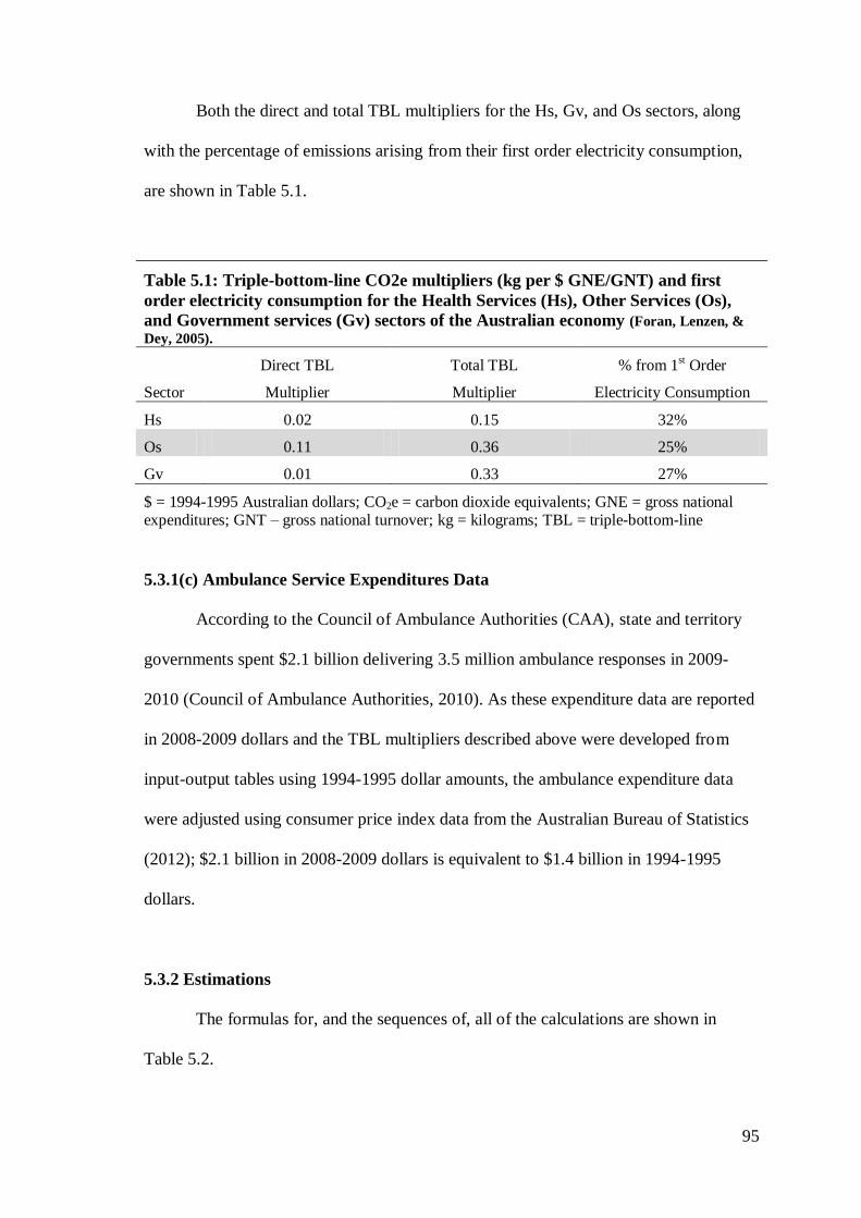
95

Both the direct and total TBL multipliers for the Hs, Gv, and Os sectors, along

with the percentage of emissions arising from their first order electricity consumption,

are shown in Table 5.1.

Table 5.1: Triple-bottom-line CO2e multipliers (kg per $ GNE/GNT) and first

order electricity consumption for the Health Services (Hs), Other Services (Os),

and Government services (Gv) sectors of the Australian economy (Foran, Lenzen, &

Dey, 2005).

Sector

Direct TBL

Multiplier

Total TBL

Multiplier

% from 1st Order

Electricity Consumption

Hs 0.02 0.15 32%

Os 0.11 0.36 25%

Gv 0.01 0.33 27%

$ = 1994-1995 Australian dollars; CO2e = carbon dioxide equivalents; GNE = gross national expenditures; GNT – gross national turnover; kg = kilograms; TBL = triple-bottom-line

5.3.1(c) Ambulance Service Expenditures Data

According to the Council of Ambulance Authorities (CAA), state and territory

governments spent $2.1 billion delivering 3.5 million ambulance responses in 2009-

2010 (Council of Ambulance Authorities, 2010). As these expenditure data are reported

in 2008-2009 dollars and the TBL multipliers described above were developed from

input-output tables using 1994-1995 dollar amounts, the ambulance expenditure data

were adjusted using consumer price index data from the Australian Bureau of Statistics

(2012); $2.1 billion in 2008-2009 dollars is equivalent to $1.4 billion in 1994-1995

dollars.

5.3.2 Estimations

The formulas for, and the sequences of, all of the calculations are shown in

Table 5.2.

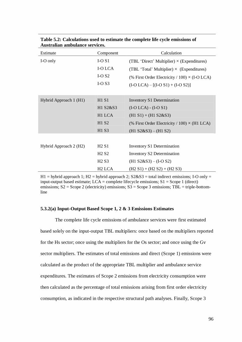
96

Table 5.2: Calculations used to estimate the complete life cycle emissions of

Australian ambulance services.

Estimate Component Calculation

I-O only I-O S1

I-O LCA

I-O S2

I-O S3

(TBL ‘Direct’ Multiplier) × (Expenditures)

(TBL ‘Total’ Multiplier) × (Expenditures)

(% First Order Electricity / 100) × (I-O LCA)

(I-O LCA) – [(I-O S1) + (I-O S2)]

Hybrid Approach 1 (H1) H1 S1

H1 S2&S3

H1 LCA

H1 S2

H1 S3

Inventory S1 Determination

(I-O LCA) - (I-O S1)

(H1 S1) + (H1 S2&S3)

(% First Order Electricity / 100) × (H1 LCA)

(H1 S2&S3) – (H1 S2)

Hybrid Approach 2 (H2)

H2 S1

H2 S2

H2 S3

H2 LCA

Inventory S1 Determination

Inventory S2 Determination

(H1 S2&S3) – (I-O S2)

(H2 S1) + (H2 S2) + (H2 S3)

H1 = hybrid approach 1; H2 = hybrid approach 2; S2&S3 = total indirect emissions; I-O only = input-output based estimate; LCA = complete lifecycle emissions; S1 = Scope 1 (direct)

emissions; S2 = Scope 2 (electricity) emissions; S3 = Scope 3 emissions; TBL = triple-bottom-

line

5.3.2(a) Input-Output Based Scope 1, 2 & 3 Emissions Estimates

The complete life cycle emissions of ambulance services were first estimated

based solely on the input-output TBL multipliers: once based on the multipliers reported

for the Hs sector; once using the multipliers for the Os sector; and once using the Gv

sector multipliers. The estimates of total emissions and direct (Scope 1) emissions were

calculated as the product of the appropriate TBL multiplier and ambulance service

expenditures. The estimates of Scope 2 emissions from electricity consumption were

then calculated as the percentage of total emissions arising from first order electricity

consumption, as indicated in the respective structural path analyses. Finally, Scope 3

97

emissions were then calculated as the difference between total emissions and the sum of

Scope 1 and Scope 2 emissions.

5.3.2(b) Hybrid Approach 1: Inventory Based Scope 1 and Input-Output Based

Scope 2 & 3 Emissions

The first set of hybrid estimates (H1) of ambulance service life cycle emissions

assumed that the inventory-based determination of direct emissions was more accurate

than the input-output based determinations. For these estimates, the inventory-based

determination was used for Scope 1 emissions, while the Hs, Os and Gv TBL

multipliers were each used to estimate indirect emissions. Scope 2 emissions from

electricity were again estimated as the percentage of total emissions reported for first

order electricity consumption in the existing structural path analyses.

5.3.2(c) Hybrid Approach 2: Inventory Based Scope 1 & 2 and Input-Output

Based Scope 3 Emissions

The second set of hybrid estimates (H2) of ambulance service life cycle

emissions assumed that the inventory-based determinations of both direct emissions and

electricity-related emissions were more accurate than the input-output based

determinations. For these estimates, the inventory-based determinations were used for

both direct (Scope 1) and electricity (Scope 2) emissions. Scope 3 emissions were

calculated as the difference between the indirect emissions calculated in the H1

estimates and the electricity emissions estimated using the pure input-output approach.

98

5.4 Ethical Review

The HREC at James Cook University approved this study (HREC #H4277,

Appendix 1) with the understanding that all data and analyses be reported in the

aggregate.

5.5 Results

Table 5.3 shows the results of the emissions estimates, as well as the average of

all the estimates.

The estimates of annual complete life cycle emissions from Australian

ambulance services range from 216,369 t CO2e to 546,688 t CO2e; the average of these

estimates is 389,315 t CO2e. On a per-event basis, estimated emissions range from

approximately 60kg CO2e per ambulance response to 150 kg CO2e per ambulance

response, with an average of 110 kg CO2e per ambulance response. In all of the

estimates, the contribution of indirect emissions is substantial, ranging from 63% to

97% of total emissions. On average, indirect (Scope 2 and Scope 3) emissions account

for 80% of total estimated emissions.

Figure 5.2 provides a visual display of the emissions estimates. The lowest

estimates of complete life cycle emissions from Australian ambulance systems arise

from the calculations incorporating TBL multipliers from the Hs sector; emissions

estimates based on the Os and GV TBL multipliers are approximately 1.5 to 2.4 times

greater than those based on the Hs TBL multipliers, depending on the estimation

procedure.

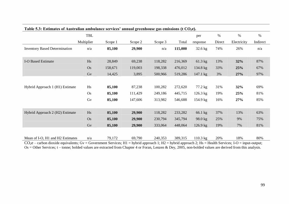
99

Table 5.3: Estimates of Australian ambulance services’ annual greenhouse gas emissions (t CO2e).

TBL

Multiplier

Scope 1

Scope 2

Scope 3

Total

per

response

%

Direct

%

Electricity

%

Indirect

Inventory Based Determination n/a 85,100 29,900 n/a 115,000 32.6 kg 74% 26% n/a

I-O Based Estimate Hs 28,849 69,238 118,282 216,369 61.3 kg 13% 32% 87%

Os 158,671 119,003 198,338 476,012 134.8 kg 33% 25% 67%

Gv 14,425 3,895 500,966 519,286 147.1 kg 3% 27% 97%

Hybrid Approach 1 (H1) Estimate Hs 85,100 87,238 100,282 272,620 77.2 kg 31% 32% 69%

Os 85,100 111,429 249,186 445,715 126.3 kg 19% 25% 81%

Gv 85,100 147,606 313,982 546,688 154.9 kg 16% 27% 85%

Hybrid Approach 2 (H2) Estimate Hs 85,100 29,900 118,282 233,282 66.1 kg 37% 13% 63%

Os 85,100 29,900 230,794 345,794 98.0 kg 25% 9% 75%

Gv 85,100 29,900 333,064 448,064 126.9 kg 19% 7% 81%

Mean of I-O, H1 and H2 Estimates n/a 79,172 69,790 240,353 389,315 110.3 kg 20% 18% 80%

CO2e – carbon dioxide equivalents; Gv = Government Services; H1 = hybrid approach 1; H2 = hybrid approach 2; Hs = Health Services; I-O = input-output;

Os = Other Services; t – tonne; bolded values are extracted from Chapter 4 or Foran, Lenzen & Dey, 2005, non-bolded values are derived from this analysis.

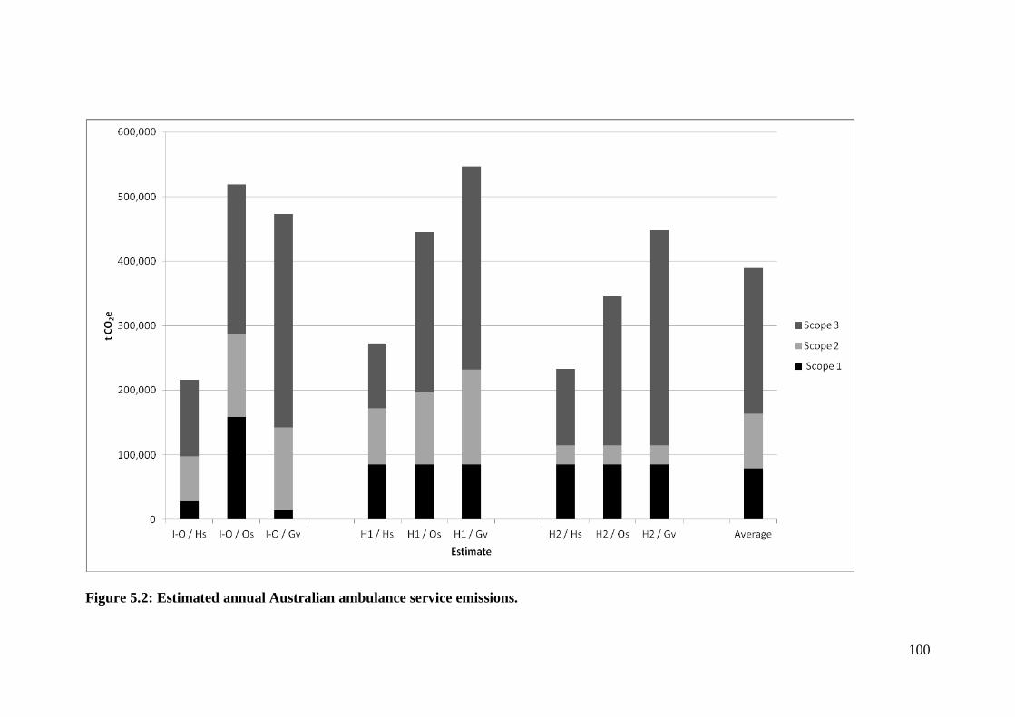
100

Figure 5.2: Estimated annual Australian ambulance service emissions.

101

Regardless of the TBL multipliers used, including the inventory-based

determination of Scope 2 emissions substantially reduces the proportion of estimated

emissions arising from first order electricity consumption. The structural path analyses

suggest first order electricity consumption would be responsible for 25% to 32% of total

ambulance service emissions; using the inventory based determination of Scope 2

emissions reduces those proportions to between 7% and 13%. On average, electricity

consumption is responsible for 18% of estimated ambulance service emissions.

Table 5.4 shows the top five structural pathways for the three economic sectors

used in this analysis; in all of these sectors, zero order transactions within the sector and

first order electricity consumption are among the top five structural paths. The

remaining leading structural paths include some that would be intuitively related to

ambulance services—such as chemicals, wholesale trade, and paper products—as well

as some that are not intuitive. This is particularly true within the Os sector, where

‘lime’, ‘sheep and shorn wool’ and ‘beef cattle for meat products’ are among the

leading structural paths. The top five structural paths account for 53%, 63%, and 37% of

emissions estimated using only the input-output based TBL multipliers for the Hs, Os

and Gv sectors, respectively.

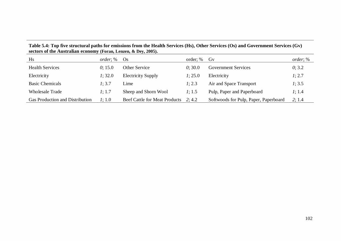
102

Table 5.4: Top five structural paths for emissions from the Health Services (Hs), Other Services (Os) and Government Services (Gv)

sectors of the Australian economy (Foran, Lenzen, & Dey, 2005).

Hs order; % Os order; % Gv order; %

Health Services

Electricity

Basic Chemicals

Wholesale Trade

Gas Production and Distribution

0; 15.0

1; 32.0

1; 3.7

1; 1.7

1; 1.0

Other Service

Electricity Supply

Lime

Sheep and Shorn Wool

Beef Cattle for Meat Products

0; 30.0

1; 25.0

1; 2.3

1; 1.5

2; 4.2

Government Services

Electricity

Air and Space Transport

Pulp, Paper and Paperboard

Softwoods for Pulp, Paper, Paperboard

0; 3.2

1; 2.7

1; 3.5

1; 1.4

2; 1.4

103

5.6 Discussion

In the 2009-2010 financial year, Australia’s national expenditures on health care

totalled $121.4 billion dollars (Australian Institute of Health and Welfare, 2011).

Converting this sum to 1994-1995 dollars and applying the health services TBL total

emissions multiplier indicates Australian health services were responsible for

approximately 12.3 million t of CO2e emissions in the 2009-2010 financial year. Using

the average estimate from this analysis suggests that ambulance services were

responsible for 3.2% of all Australian health sector emissions in that year; the best case

and worst case estimates of ambulance service emissions are 1.8% and 4.4% of total

health sector emissions, respectively. Since ambulance service expenditures ($2.1

billion) represent 1.7% of total health expenditures, all except the most conservative

estimates indicate that ambulance services are a disproportionate contributor to health

sector emissions. As such, they might play an important role in reducing health sector

emissions.

Reducing emissions from vehicle fuel consumption is probably the most obvious

strategy ambulance systems could employ to reduce their carbon footprint. In this

analysis, direct emissions—primarily from diesel, petrol and aviation fuels—accounted

on average for only 20% of all ambulance system emissions. However, when using the

inventory based Scope 1 and Scope 2 emissions and assuming that input-output based

Scope 3 emissions of ambulance services are consistent with those of the Hs sector (that

is, when using the ‘H2 / Hs’ estimate in Table 5.3 and Figure 5.2), the contribution of

emissions from vehicle fuels could be as high as 37% of total emissions. At 3.5 million

ambulance responses per year, even marginal reductions in emissions from each

individual ambulance response could result in substantial cumulative emissions

reductions. Strategies for reducing vehicle fuel consumption and Scope 1 emissions

104

could include reducing ambulance idling time at emergency scenes and receiving

hospitals, transitioning to higher efficiency vehicle fleets, and limiting the use of

medical helicopters to only those emergency situations in which they have been shown

to improve patient outcomes.

Other strategies for reducing ambulance system Scope 1 emissions would mirror

those of the broader transportation sector. Conversion to bio-diesel as a vehicle fuel

would reduce direct emissions, although the complete life cycle emissions of bio-fuels

are not necessarily significantly less than those of fossil-based liquid fuels (Nanaki &

Koroneos, 2012; Solomon, 2010; von Blottnitz & Curran, 2007). For example, in

Australia low sulphur diesel emissions are only marginally greater than emissions from

‘E15D diesohol’ (a blend of low sulphur diesel and 15% ethanol): 925 g CO2e / km

versus 862 g CO2e / km (Beer & Grant, 2007). Bio-fuels are also often associated with

other detrimental environmental and land use effects (Lange, 2011; Nanaki &

Koroneos, 2012; Solomon, 2010; von Blottnitz & Curran, 2007).

Another potential strategy is to transition to a more efficient ambulance and

support vehicle fleet. Plug-in hybrid electric vehicles (PHEVs) are one option, but

depending on the fuel source for electricity generation, they might simply shift Scope 1

greenhouse gas emissions to Scope 2 emissions. A case study from Milan, Italy,

asserted that thermal power stations in that region were efficient enough to justify the

introduction of electric vehicles into the private vehicle fleet, although they could

dramatically increase peak electricity demand (Perujo & Ciuffo, 2010). Sioshansi,

Fagiani, & Marano (2010) came to the same conclusion for PHEVs in Ohio despite that

U.S. state’s high concentration of coal-fired power plants, although emissions of

sulphur dioxide and nitrogen oxides were substantially higher for PHEVs compared to

conventional vehicles. An analysis from California also found that PHEVs—as well as

105

battery electric vehicles (BEVs)—would produce lower complete life cycle greenhouse

gas emissions than both conventional and hybrid internal combustion engines

(McCarthy & Yang, 2010). To my knowledge, an assessment of the environmental

impacts of PHEVs in Australia has not been reported.

Hydrogen fuel cell vehicles (FCVs) are another option for both support and

transport vehicles, but again the process of hydrogen production can profoundly impact

their life cycle emissions (Ozalp, Epstein, & Kogan, 2010; Pro, Hammerschlag, &

Mazza, 2005). In New Zealand, Leaver & Gillingham (2010) estimated that FCVs,

along with BEVs, would be the best alternative vehicle technologies for reducing

greenhouse gas emissions. In London, FCV taxis have lower complete life cycle energy

consumption and emissions than diesel and BEV taxis (Baptista et al., 2011). On the

contrary, in the U.S. state of California, McCarthy & Yang (2010) predicted FCVs

would produce more greenhouse gas emissions than conventional or hybrid internal

combustion engines given current electricity and hydrogen generation processes. A

further immediate limitation on FCVs is the lack of a sufficient hydrogen distribution

and refuelling infrastructure (Vergragt & Brown, 2007).

Reducing emissions from electricity consumption is another way in which

ambulance services could reduce their environmental impact. In this analysis, electricity

consumption accounted on average for 22% of total ambulance system emissions. In

contrast to the data for Scope 1 emissions, using the inventory based determinations of

electricity-related emissions reduced their contribution to the total carbon footprint of

ambulance systems. This makes sense: while ambulance systems must maintain some

administrative office space and facilities for housing ambulances and staff, they are

primarily mobile services. Even the most optimistic estimate in this analysis, however,

would put electricity-related emissions at 7% of total emissions, which would still make

106

first order electricity consumption a leading structural path for ambulance service

emissions.

Conservation efforts aimed at reducing electricity consumption could directly

reduce the Scope 2 emissions of ambulance services, but advocating for ‘green’

electricity generation could have an even more profound indirect impact. All of the

estimates in this analysis indicate that upstream Scope 3 emissions are the largest

contributor to ambulance system emissions. Reducing the emissions intensity of

electricity production could reduce not only the electricity-related Scope 2 emissions of

ambulance services, but also the upstream Scope 3 emissions associated with electricity

consumption in the supply chain.

Implementing environmentally friendly purchasing practices would further

reduce ambulance system life cycle emissions. In this analysis, Scope 3 emissions

represent nearly 60% of ambulance services’ complete life cycle emissions. This is

consistent with previous data showing that indirect emissions constitute the majority of

emissions arising from service sectors and service industries (Larsen & Hertwich, 2011;

Nansai et al., 2009; Suh, 2006).

The leading structural paths in the Hs, Os and Gv sectors provide some insights

into the products and services that ambulance services might target in those efforts. In

the absence of a more detailed analysis of ambulance system purchases, it should not be

presumed that the leading structural paths for ambulance services more closely resemble

those of the Hs or Gv sectors simply because they seem more intuitive than those of the

Os sector. Ambulance services should consider the potential benefits of reducing their

consumption of, and pursuing environmentally friendly purchasing practices for,

products in all of these paths. One aspect of complete life cycle emissions unique to

transport systems is the end-of-life management of vehicles (Manomaivibool, 2008).

107

While the greenhouse gas emissions and environmental impacts of decommissioning

ambulances and other vehicles might technically accrue to the manufacturers of those

vehicles, ambulance systems should none-the-less pursue and promote environmentally

friendly vehicle disposal.

5.7 Limitations

Admittedly, these structural paths might not represent the actual leading

structural paths for ambulance services. This study did not incorporate an inventory of

ambulance service purchases and, as the Scope 1 and Scope 2 data demonstrate, the

aggregate TBL multipliers and structural paths for the Hs, Os, and Gv sectors might not

accurately reflect the true environmental impact of Australian ambulance systems. This

is a common limitation of top-down estimates of carbon footprints and structural path

analyses using aggregate sectoral input-output based multipliers (Baboulet & Lenzen,

2010; Lenzen, Pade, & Munksgaard, 2004; Su, Huang, Ang, & Zhou, 2010). This

analysis further highlights how the problem might be even more pronounced for

activities that organisationally fit within one economic sector, but that are operationally

more similar to activities in other economic sectors.

Ideally, estimating the complete life cycle emissions of Australian ambulance

services would incorporate not only an inventory of their Scope 1 and Scope 2 energy

consumption, but also an inventory of their purchases from which more specific input-

output based estimates of Scope 3 emissions could be made. Unfortunately, that was not

logistically possible for this analysis. Even if it had been possible, the study would still

be limited in that the input-output tables used to construct the TBL multipliers were

from 1994-1995 (Foran, Lenzen, & Dey, 2005). Thus this analysis, and any analysis

using those multipliers, assumes that production processes and inter-sectoral

108

transactions in the Australian economy have not changed substantially in the last 15

years. This too, is a common shortcoming of input-output based analyses (Foran,

Lenzen, & Dey, 2005; Lenzen 2002; Su, Huang, Ang, & Zhou, 2010). These are none-

the-less the most recent TBL multipliers publicly available for the Australian economy.

For both these reasons, and consistent with the ISO recommendations for life

cycle analysis, these data are more useful as a starting point for tracking ambulance

service emissions—and changes in those emissions—over time, rather than as an

accurate point estimate of ambulance service emissions (Finkbeiner, Inaba, Tan,

Christiansen, & Kluppel, 2006). In that context, any information bias resulting from the

limitations of the aggregate input-output multipliers would be a non-differential

information bias, and thus a bias towards the null hypothesis (of no change) when

comparing year-over-year greenhouse gas emissions.

Another limitation of this analysis is that it essentially uses ‘Scope 2’ emissions

and ‘electricity-related’ emissions synonymously. This is not technically correct: the

direct emissions of other purchased services, most notably travel on commercial

airlines, are also considered Scope 2 emissions. In the case of ambulance services, these

additional Scope 2 emissions are poorly tracked (Blanchard & Brown, 2011; see also

Chapter 4) but they should be relatively small. Also, in this analysis, those emissions are

still represented in the calculations of indirect and Scope 3 emissions; that is, they might

be misclassified, but they are not omitted.

Finally, this study uses aggregate expenditure data for Australian EMS systems,

and does not differentiate between ground and air ambulance activities. As

demonstrated in Chapter 4, the direct emissions associated with the consumption of

aviation fuels for air ambulance activities are substantially higher than those from

ground ambulances. The results of this study must be considered in the context of both

109

ground and air ambulance activities, and should not be misinterpreted as being specific

to ground ambulance operations.

5.8 Conclusion

This analysis used the previous inventory of Scope 1 and Scope 2 emissions

from Australian ambulance services, along with publicly available expenditure data and

input-output based TBL multipliers, to estimate the complete life cycle emissions of

Australian ambulance services. Complete life cycle emissions from Australian

ambulance services are estimated at between 216,000 and 547,000 t CO2e annually.

Ambulance services are responsible for between 1.8% and 4.4% of total Australian

health sector emissions, and can play an important role in reducing health sector

emissions. Scope 3 emissions are responsible for the majority of ambulance service

emissions, but direct emissions from vehicle fuels including diesel, petrol and aviation

fuel represent approximately 20% (and perhaps as much as 37%) of total ambulance

system emissions and are an obvious target for reducing the environmental impact of

ambulance systems.

While this chapter and the previous chapter have focused on the environmental

burden associated ambulance systems, there are other reasons to manage energy

consumption. The next chapter explores one of these reasons: the impact of energy costs

on ambulance systems.

110

Chapter 6: Energy Costs and Australian EMS Systems

Chapter 4 inventoried the Scope 1 and Scope 2 greenhouse gas emissions of

Australian ambulance services, and Chapter 5 made an estimate of their complete life

cycle emissions. Environmental concerns, however, are not the only reason to manage

energy consumption. This chapter explores the potential importance of energy scarcity

and rising energy costs for Australian ambulance services (Figure 6.1).

This chapter has been adapted into a manuscript: Brown, L.H., Chaiechi, T.,

Buettner, P.G., Canyon, D.V., Crawford, J.M., Judd, J. (Under Review). How do energy

prices impact ambulance services? Evidence from Australia.

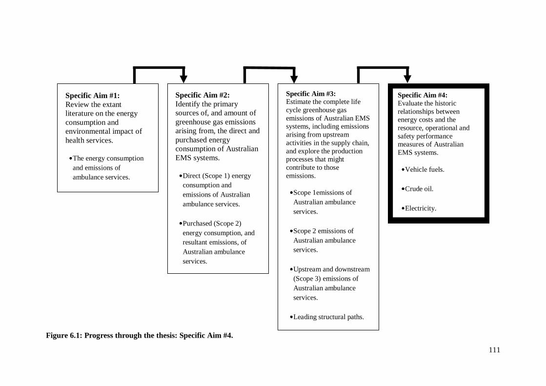
111

Figure 6.1: Progress through the thesis: Specific Aim #4.

Specific Aim #1:

Review the extant

literature on the energy

consumption and

environmental impact of

health services.

The energy consumption

and emissions of

ambulance services.

Specific Aim #3: Estimate the complete life

cycle greenhouse gas

emissions of Australian EMS systems, including emissions

arising from upstream

activities in the supply chain,

and explore the production processes that might

contribute to those

emissions.

Scope 1emissions of

Australian ambulance

services.

Scope 2 emissions of

Australian ambulance

services.

Upstream and downstream

(Scope 3) emissions of

Australian ambulance

services.

Leading structural paths.

Specific Aim #2:

Identify the primary

sources of, and amount of

greenhouse gas emissions

arising from, the direct and

purchased energy

consumption of Australian

EMS systems.

Direct (Scope 1) energy

consumption and

emissions of Australian

ambulance services.

Purchased (Scope 2)

energy consumption, and

resultant emissions, of

Australian ambulance

services.

Specific Aim #4:

Evaluate the historic

relationships between energy costs and the

resource, operational and

safety performance measures of Australian

EMS systems.

Vehicle fuels.

Crude oil.

Electricity.

112

6.1 Abstract

Concerns about the impacts of energy scarcity and rising energy prices on health

services are increasing, and there are multiple reports in the lay media specifically

warning of the adverse effects of fuel price hikes on ambulance services. This study

empirically evaluates the impact of historical energy price fluctuations on Australian

ambulance services. A panel data approach is used to investigate the effect of energy

prices on ambulance system resource, operational and safety performance measures.

The data reveal an inverse relationship between fuel prices and ambulance service

resources, and a one-year lagged association between increases in fuel prices and longer

response times. There is also a positive association between electricity prices and

workplace injury compensation claims.

6.2 Introduction

The potential adverse impacts of rising energy prices on health services are the

subject of much opinion, but little empirical evaluation. Three decades ago, noting that

health facilities are dependent on energy, Bailey (1980) raised concerns about energy

scarcity and energy costs in the context of the U.S. dependence on imported oil. More

recently, several authors have warned of the threats posed to all health systems by

global peak oil. They argue that energy is a critical input for health services (Frumkin,

Hess, and Vindigni, 2007; 2009; Hanlon & McCartney, 2008; Hess, Bednarz, Bae, &

Pierce, 2011; Schwartz, Parker, Hess, & Frumkin, 2011; Wilkinson, 2008; Winch &

Stepnitz, 2011) and that there are several pathways through which energy scarcity and

energy costs could affect health services, including: the cost and availability of medical

supplies and equipment; the cost and availability of health-related transport; the cost of

lighting, heating and air conditioning health facilities; impacts on food security leading

113

to increased demand on health services; and economic impacts that disrupt funding for

health services (Clark & Kline, 1981; Frumkin, Hess, & Vindigni, 2009; Winch &

Stepnitz, 2011). These concerns are shared by the general public. In a 2009-2010 survey

of U.S. adults, 48% said they anticipated a tripling of oil prices over the next five years,

and 44% said those price increases would be harmful to health (Nisbet, Maibach, &

Leiserowitz, 2011). There is some, albeit minimal, empirical basis for these concerns. In

a time series analysis of U.S. petroleum and health care prices between 1973 and 2008,

Hess et al. (2011) found a 1% increase in oil price inflation was associated with a 0.03%

increase in medical care prices after an eight month lag. This price elevation persisted

for 20 months, although the effect was much stronger in the 1970s than in recent years.

Ambulance services are an integral component of the health care system

(Delbridge et al., 1998). Recent reports in the lay media have anecdotally described the

adverse effects of rising fuel costs on the operating budgets of these services

(Anonymous, 2011; Fallon, 2011; Harlin, 2009; Odell, 2011; Penner, 2008), but the

extent of those impacts and how they manifest have not been empirically studied.

Ambulance services are complex systems involving vehicles, equipment, buildings,

communication systems and personnel (Lerner, Nichol, Spaite, Garrison, & Maio,

2007), and increasing energy costs could conceivably impact any or all of these system

components. This study evaluates the impact of historical energy price fluctuations on

Australian ambulance services, using a panel data approach to test the null hypothesis

that ambulance service resource, operational and safety performance characteristics are

not associated with energy prices.

114

6.3 Methodology

6.3.1 Setting

In Australia, responsibility for ambulance services rests with state and territory

governments. In NSW, SA, and TAS ambulance services are provided by the

Department of Health. In QLD and the ACT ambulance services are provided by the

departments responsible for emergency services. St. John’s Ambulance Service, an

independent not-for-profit organisation, is contracted to provide services in NT and

WA. In VIC, ambulance services are now organised within the Department of Health,

but prior to 2008 they were provided by two independent statutory authorities: the

Metropolitan Ambulance Service (MAS) serving the greater Melbourne area, and Rural

Ambulance Victoria (RAV) serving the remainder of the state. In the 2009-2010

financial year, Australian ambulance services performed slightly more than 3.5 million

emergency and non-emergency responses (Council of Ambulance Authorities, 2010).

6.3.2 Design

This was a retrospective study using a panel data approach to evaluate the

historical relationships between energy prices and resource allocation, as well as

operational and safety performance measures, in Australian ambulance agencies.

6.3.3 Data Sources

6.3.3(a) Ambulance Service Data

Data on the resource, operational and safety characteristics of the ambulance

services in Australia’s six states were obtained from publicly available annual reports

published online at each agency’s website, or its parent agency’s (e.g., Department of

Health) website. While Ambulance-Victoria data for the entire state of VIC were

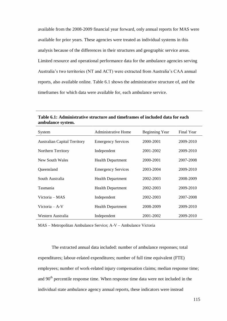
115

available from the 2008-2009 financial year forward, only annual reports for MAS were

available for prior years. These agencies were treated as individual systems in this

analysis because of the differences in their structures and geographic service areas.

Limited resource and operational performance data for the ambulance agencies serving

Australia’s two territories (NT and ACT) were extracted from Australia’s CAA annual

reports, also available online. Table 6.1 shows the administrative structure of, and the

timeframes for which data were available for, each ambulance service.

Table 6.1: Administrative structure and timeframes of included data for each

ambulance system.

System Administrative Home Beginning Year Final Year

Australian Capital Territory Emergency Services 2000-2001 2009-2010

Northern Territory Independent 2001-2002 2009-2010

New South Wales Health Department 2000-2001 2007-2008

Queensland Emergency Services 2003-2004 2009-2010

South Australia Health Department 2002-2003 2008-2009

Tasmania Health Department 2002-2003 2009-2010

Victoria – MAS Independent 2002-2003 2007-2008

Victoria – A-V Health Department 2008-2009 2009-2010

Western Australia Independent 2001-2002 2009-2010

MAS – Metropolitan Ambulance Service; A-V – Ambulance Victoria

The extracted annual data included: number of ambulance responses; total

expenditures; labour-related expenditures; number of full time equivalent (FTE)

employees; number of work-related injury compensation claims; median response time;

and 90th

percentile response time. When response time data were not included in the

individual state ambulance agency annual reports, these indicators were instead

116

extracted from the CAA annual reports. Lastly, CAA also conducts an annual

nationwide patient satisfaction survey from which reported satisfaction with ambulance

response times (on a scale of 0 to 100), beginning with the 2003-2004 financial year,

was also extracted. In some cases, prior year data were reported in the first available

report, allowing collection (or calculation) of data for one additional year.

From these data, nine performance measures were identified or calculated: four

resource performance indicators, three operational performance indicators, and two

safety performance indicators. Table 6.2 describes each performance indicator in detail.

6.3.3(b) Energy Price Data

The Australian Institute of Petroleum (AIP) reports annual average terminal gate

prices (TGP) for diesel fuel and petrol in Australia’s capital cities, with the exception of

Canberra, ACT. TGP reflects the wholesale price of diesel or petrol with goods and

services tax added. TGP data for diesel fuel for financial years 2004-2005 through

2009-2010 were obtained from the AIP website (Australian Institute of Petroleum,

2010), and the annual average TGP for diesel fuel in each capital city (as cents per L)

was used as a measure of vehicle fuel prices for each state or territory. The annual

average TGP for Sydney, NSW was used as a proxy measure for the cost of diesel in the

ACT.

State average annual electricity prices (as dollars per megawatt hour) for

financial years 2000-2001 through 2009-2010 were obtained from the Australian

Energy Market Operator (AEMO) (Australian Energy Market Operator, 2010). AEMO

data for TAS were limited to the 2004-2005 through 2009-2010 financial years, and the

AEMO data does not include electricity price data for WA, NT, or ACT. Electricity

prices for NSW were used as a proxy for electricity prices in ACT, but because of their

117

remoteness, distinctive geography and unique economies, a proxy measure of electricity

prices for NT and WA was not attempted.

Since TGP data were available for only six financial years, average annual world

crude oil prices were used as an additional indirect measure of vehicle fuel costs with a

longer historical record. Oil prices were obtained from the U.S. EIA’s reported world

weekly average crude oil prices for financial years 2000-2001 through 2009-2010 (U.S.

Energy Information Administration, 2011). Since these EIA data are reported in U.S.

dollars, annual average exchange rates reported by the Australian Tax Office

(Australian Tax Office, 2011) were used to convert these prices into Australian dollar

prices (as dollars per barrel).

6.3.4 Analysis

6.3.4(a) Model Selection

The panel data analysis followed the approaches outlined by Markus (1979),

Hsiao (1986) and Twisk (2003). Generalised Estimating Equation (GEE) modelling was

used to evaluate the relationships between the energy price measures and the system

performance measures while accounting for the repeated-measures nature of the

performance measures. GEE modelling, which was initially proposed by Liang & Zeger

(1986) and Zeger & Liang (1986), considers a two-part estimating equation that

simultaneously estimates (1) the regression parameters and (2) the parameters of the

second order variance distribution. Thus, in GEE the relationships between the variables

in the model at different time points are analysed simultaneously (Liang and Zeger

1986; Twisk, 2003); conceptually it can be thought of as regression modelling with

correction for the dependency of the serial observations (Burton, Gurrin, & Sly, 1998).

GEE models generate robust and model-based standard errors, and produce consistent

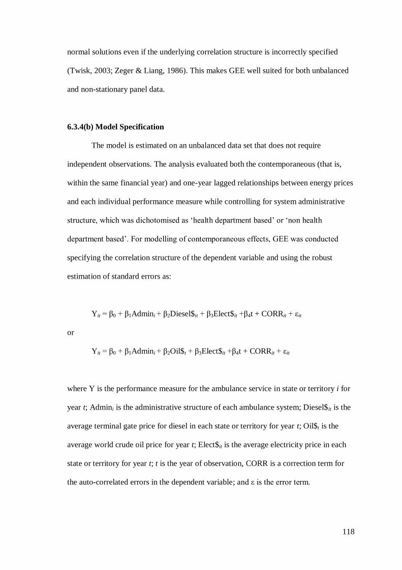
118

normal solutions even if the underlying correlation structure is incorrectly specified

(Twisk, 2003; Zeger & Liang, 1986). This makes GEE well suited for both unbalanced

and non-stationary panel data.

6.3.4(b) Model Specification

The model is estimated on an unbalanced data set that does not require

independent observations. The analysis evaluated both the contemporaneous (that is,

within the same financial year) and one-year lagged relationships between energy prices

and each individual performance measure while controlling for system administrative

structure, which was dichotomised as ‘health department based’ or ‘non health

department based’. For modelling of contemporaneous effects, GEE was conducted

specifying the correlation structure of the dependent variable and using the robust

estimation of standard errors as:

Yit = β0 + β1Admini + β2Diesel$it + β3Elect$it +β4t + CORRit + εit

or

Yit = β0 + β1Admini + β2Oil$t + β3Elect$it +β4t + CORRit + εit

where Y is the performance measure for the ambulance service in state or territory i for

year t; Admini is the administrative structure of each ambulance system; Diesel$it is the

average terminal gate price for diesel in each state or territory for year t; Oil$t is the

average world crude oil price for year t; Elect$it is the average electricity price in each

state or territory for year t; t is the year of observation, CORR is a correction term for

the auto-correlated errors in the dependent variable; and ε is the error term.

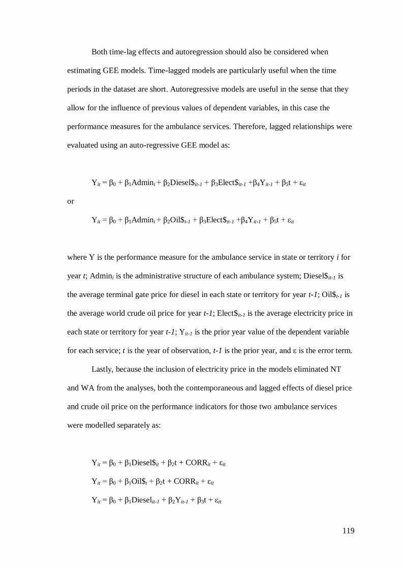
119

Both time-lag effects and autoregression should also be considered when

estimating GEE models. Time-lagged models are particularly useful when the time

periods in the dataset are short. Autoregressive models are useful in the sense that they

allow for the influence of previous values of dependent variables, in this case the

performance measures for the ambulance services. Therefore, lagged relationships were

evaluated using an auto-regressive GEE model as:

Yit = β0 + β1Admini + β2Diesel$it-1 + β3Elect$it-1 +β4Yit-1 + β5t + εit

or

Yit = β0 + β1Admini + β2Oil$t-1 + β3Elect$it-1 +β4Yit-1 + β5t + εit

where Y is the performance measure for the ambulance service in state or territory i for

year t; Admini is the administrative structure of each ambulance system; Diesel$it-1 is

the average terminal gate price for diesel in each state or territory for year t-1; Oil$t-1 is

the average world crude oil price for year t-1; Elect$it-1 is the average electricity price in

each state or territory for year t-1; Yit-1 is the prior year value of the dependent variable

for each service; t is the year of observation, t-1 is the prior year, and ε is the error term.

Lastly, because the inclusion of electricity price in the models eliminated NT

and WA from the analyses, both the contemporaneous and lagged effects of diesel price

and crude oil price on the performance indicators for those two ambulance services

were modelled separately as:

Yit = β0 + β1Diesel$it + β2t + CORRit + εit

Yit = β0 + β1Oil$t + β2t + CORRit + εit

Yit = β0 + β1Dieselit-1 + β2Yit-1 + β3t + εit

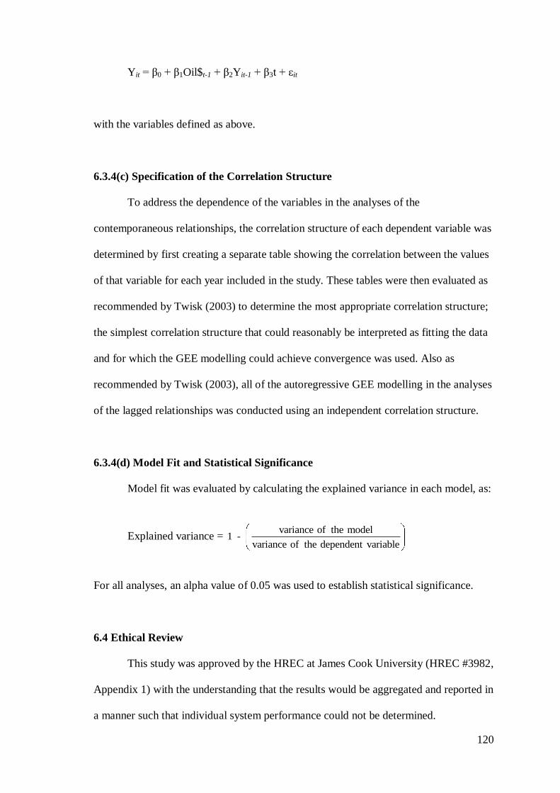
120

Yit = β0 + β1Oil$t-1 + β2Yit-1 + β3t + εit

with the variables defined as above.

6.3.4(c) Specification of the Correlation Structure

To address the dependence of the variables in the analyses of the

contemporaneous relationships, the correlation structure of each dependent variable was

determined by first creating a separate table showing the correlation between the values

of that variable for each year included in the study. These tables were then evaluated as

recommended by Twisk (2003) to determine the most appropriate correlation structure;

the simplest correlation structure that could reasonably be interpreted as fitting the data

and for which the GEE modelling could achieve convergence was used. Also as

recommended by Twisk (2003), all of the autoregressive GEE modelling in the analyses

of the lagged relationships was conducted using an independent correlation structure.

6.3.4(d) Model Fit and Statistical Significance

Model fit was evaluated by calculating the explained variance in each model, as:

Explained variance = variance of the model

1 -variance of the dependent variable

For all analyses, an alpha value of 0.05 was used to establish statistical significance.

6.4 Ethical Review

This study was approved by the HREC at James Cook University (HREC #3982,

Appendix 1) with the understanding that the results would be aggregated and reported in

a manner such that individual system performance could not be determined.

121

6.5 Results

6.5.1 General Results

During the years included in this study, Australian ambulance systems

performed more than 20 million ambulance responses, with annual median response

times ranging between 7.2 and 11.0 minutes at an average (± standard deviation)

expense of $542 $126 per response. The aggregate measures of all the performance

indicators are shown in Table 6.2.

None of these measures were reported for all ambulance systems for all years,

except for 90th percentile response time; Table 6.2 also shows the number of system-

years for which performance indicator data were available. Safety-related performance

measures were the most under-reported performance measure, available for only four

systems for a total of 20 system-years.

Figures 6.2 through 6.4 show the relationships between energy prices and the

aggregate resource, operational and safety performance measures over the years

included in the study. While similar movements in the three energy price measures are

apparent, there are no obvious associated trends in the resource, operational or safety

performance indicators.

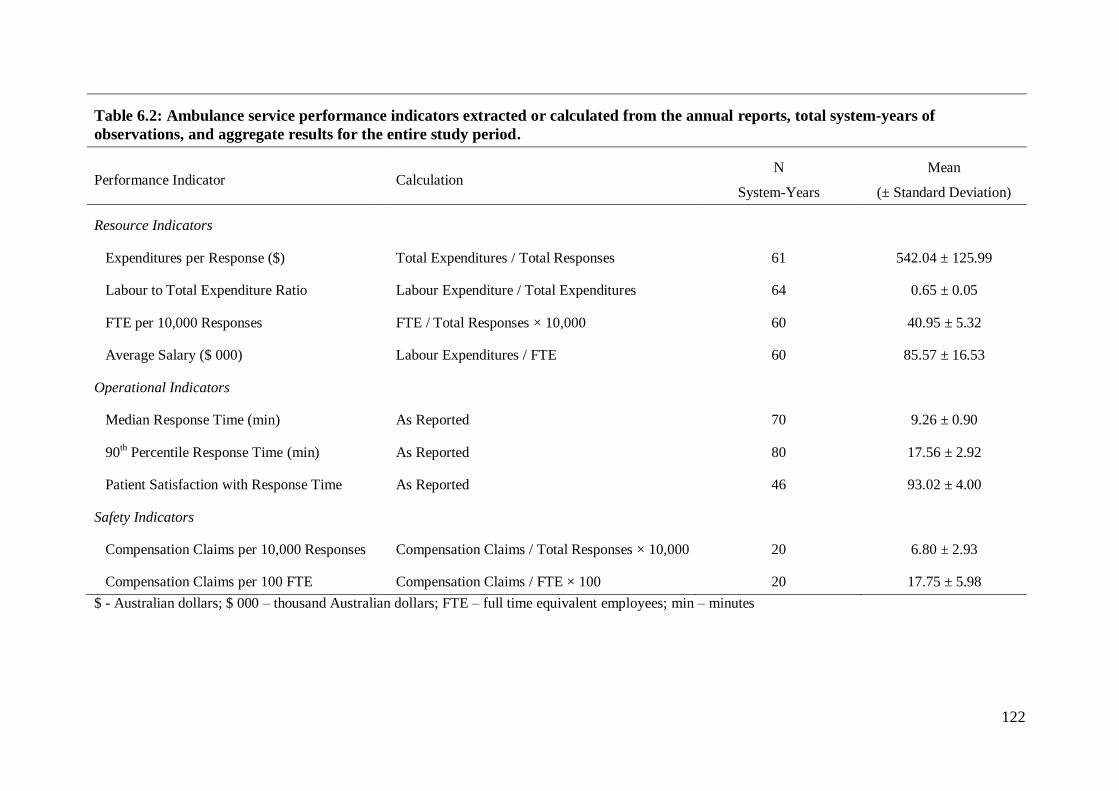
122

Table 6.2: Ambulance service performance indicators extracted or calculated from the annual reports, total system-years of

observations, and aggregate results for the entire study period.

Performance Indicator Calculation N

System-Years

Mean

(± Standard Deviation)

Resource Indicators

Expenditures per Response ($) Total Expenditures / Total Responses 61 542.04 ± 125.99

Labour to Total Expenditure Ratio Labour Expenditure / Total Expenditures 64 0.65 ± 0.05

FTE per 10,000 Responses FTE / Total Responses × 10,000 60 40.95 ± 5.32

Average Salary ($ 000) Labour Expenditures / FTE 60 85.57 ± 16.53

Operational Indicators

Median Response Time (min) As Reported 70 9.26 ± 0.90

90th Percentile Response Time (min) As Reported 80 17.56 ± 2.92

Patient Satisfaction with Response Time As Reported 46 93.02 ± 4.00

Safety Indicators

Compensation Claims per 10,000 Responses Compensation Claims / Total Responses × 10,000 20 6.80 ± 2.93

Compensation Claims per 100 FTE Compensation Claims / FTE × 100 20 17.75 ± 5.98

$ - Australian dollars; $ 000 – thousand Australian dollars; FTE – full time equivalent employees; min – minutes

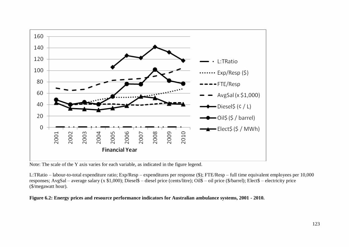
123

Note: The scale of the Y axis varies for each variable, as indicated in the figure legend.

L:TRatio – labour-to-total expenditure ratio; Exp/Resp – expenditures per response ($); FTE/Resp – full time equivalent employees per 10,000

responses; AvgSal – average salary (x $1,000); Diesel$ – diesel price (cents/litre); Oil$ – oil price ($/barrel); Elect$ – electricity price

($/megawatt hour).

Figure 6.2: Energy prices and resource performance indicators for Australian ambulance systems, 2001 - 2010.

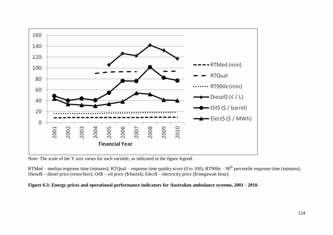
124

Note: The scale of the Y axis varies for each variable, as indicated in the figure legend.

RTMed – median response time (minutes); RTQual – response time quality score (0 to 100); RT90ile – 90th percentile response time (minutes);

Diesel$ – diesel price (cents/litre); Oil$ – oil price ($/barrel); Elect$ – electricity price ($/megawatt hour).

Figure 6.3: Energy prices and operational performance indicators for Australian ambulance systems, 2001 - 2010.

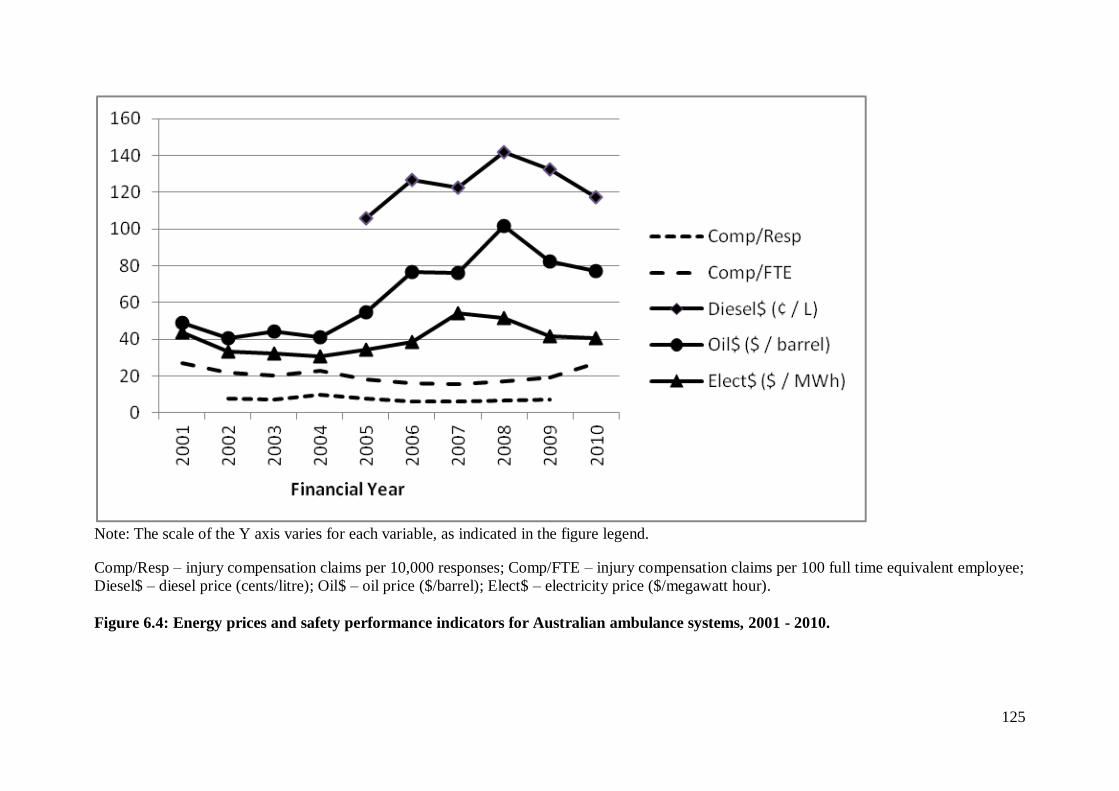
125

Note: The scale of the Y axis varies for each variable, as indicated in the figure legend.

Comp/Resp – injury compensation claims per 10,000 responses; Comp/FTE – injury compensation claims per 100 full time equivalent employee;

Diesel$ – diesel price (cents/litre); Oil$ – oil price ($/barrel); Elect$ – electricity price ($/megawatt hour).

Figure 6.4: Energy prices and safety performance indicators for Australian ambulance systems, 2001 - 2010.

126

6.5.2 Contemporaneous Effects

Table 6.3 shows the results of the GEE models evaluating contemporaneous

associations between performance indicators, time, system characteristics and energy

prices in those systems for which electricity data were available. Expenditures per

response increased over time, as did 90th percentile response times, while injury

compensation claims decreased over time. Non health-based systems had shorter

response times and fewer injury compensation claims than health-based systems.

6.5.2(a) Contemporaneous Effects of Energy Prices

Increasing diesel price was associated with decreasing ambulance service

resources: the coefficient [standard error] for expenditures per response was -2.740

[1.171]; for FTE per 10,000 responses it was -0.074 [0.020]. When using oil price

instead of diesel price in the model, the same downward effect of energy prices on

resource indicators was observed for both expenditures per response (-2.490 [0.806])

and FTE per 10,000 responses (-0.057 [0.021]).

The only statistically significant contemporaneous association between

electricity prices and the resource or operational performance indicators was a positive

association between electricity price and average salary (0.292 [0.147]) when electricity

price was modeled with diesel price. Among the safety indicators, however, increasing

electricity prices were associated with increased injury compensation claims per 100

FTE, whether electricity price was modeled with diesel price (0.201 [0.072]) or with oil

price (0.151 [0.069]) (Table 6.3).

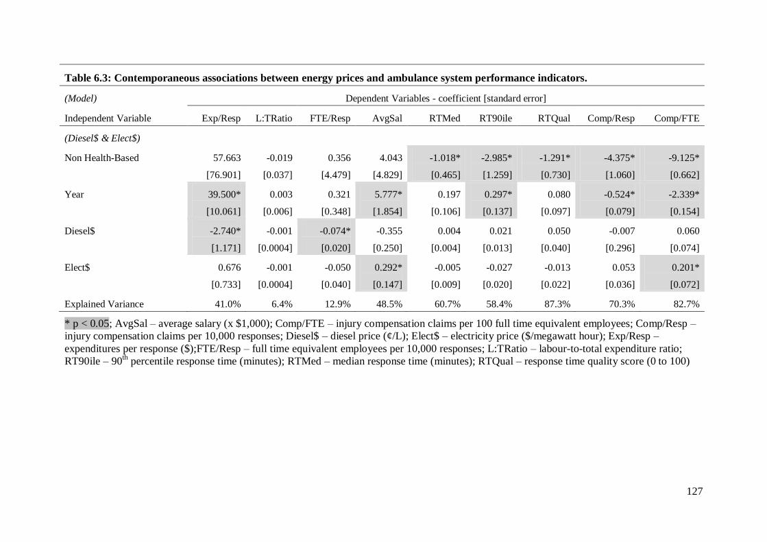
127

Table 6.3: Contemporaneous associations between energy prices and ambulance system performance indicators.

(Model) Dependent Variables - coefficient [standard error]

Independent Variable Exp/Resp L:TRatio FTE/Resp AvgSal RTMed RT90ile RTQual Comp/Resp Comp/FTE

(Diesel$ & Elect$)

Non Health-Based 57.663

[76.901]

-0.019

[0.037]

0.356

[4.479]

4.043

[4.829]

-1.018*

[0.465]

-2.985*

[1.259]

-1.291*

[0.730]

-4.375*

[1.060]

-9.125*

[0.662]

Year 39.500*

[10.061]

0.003

[0.006]

0.321

[0.348]

5.777*

[1.854]

0.197

[0.106]

0.297*

[0.137]

0.080

[0.097]

-0.524*

[0.079]

-2.339*

[0.154]

Diesel$ -2.740*

[1.171]

-0.001

[0.0004]

-0.074*

[0.020]

-0.355

[0.250]

0.004

[0.004]

0.021

[0.013]

0.050

[0.040]

-0.007

[0.296]

0.060

[0.074]

Elect$ 0.676

[0.733]

-0.001

[0.0004]

-0.050

[0.040]

0.292*

[0.147]

-0.005

[0.009]

-0.027

[0.020]

-0.013

[0.022]

0.053

[0.036]

0.201*

[0.072]

Explained Variance 41.0% 6.4% 12.9% 48.5% 60.7% 58.4% 87.3% 70.3% 82.7%

* p < 0.05; AvgSal – average salary (x $1,000); Comp/FTE – injury compensation claims per 100 full time equivalent employees; Comp/Resp –

injury compensation claims per 10,000 responses; Diesel$ – diesel price (¢/L); Elect$ – electricity price ($/megawatt hour); Exp/Resp –

expenditures per response ($);FTE/Resp – full time equivalent employees per 10,000 responses; L:TRatio – labour-to-total expenditure ratio;

RT90ile – 90th percentile response time (minutes); RTMed – median response time (minutes); RTQual – response time quality score (0 to 100)

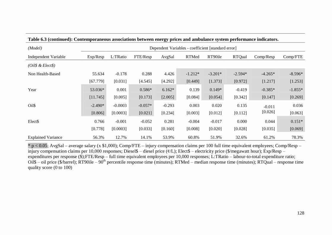
128

Table 6.3 (continued): Contemporaneous associations between energy prices and ambulance system performance indicators.

(Model) Dependent Variables - coefficient [standard error]

Independent Variable Exp/Resp L:TRatio FTE/Resp AvgSal RTMed RT90ile RTQual Comp/Resp Comp/FTE

(Oil$ & Elect$)

Non Health-Based 55.634

[67.779]

-0.178

[0.031]

0.288

[4.545]

4.426

[4.292]

-1.212*

[0.449]

-3.201*

[1.373]

-2.594*

[0.972]

-4.265*

[1.217]

-8.596*

[1.253]

Year 53.036*

[11.745]

0.001

[0.005]

0.586*

[0.173]

6.162*

[2.005]

0.139

[0.084]

0.149*

[0.054]

-0.419

[0.342]

-0.385*

[0.147]

-1.855*

[0.269]

Oil$ -2.490*

[0.806]

-0.0003

[0.0003]

-0.057*

[0.021]

-0.293

[0.234]

0.003

[0.003]

0.020

[0.012]

0.135

[0.112]

-0.011

[0.026]

0.036

[0.063]

Elect$ 0.766

[0.778]

-0.001

[0.0003]

-0.052

[0.033]

0.281

[0.160]

-0.004

[0.008]

-0.017

[0.020]

0.000

[0.028]

0.044

[0.035]

0.151*

[0.069]

Explained Variance 56.3% 12.7% 14.1% 53.9% 60.8% 51.9% 32.6% 61.2% 78.3%

* p < 0.05; AvgSal – average salary (x $1,000); Comp/FTE – injury compensation claims per 100 full time equivalent employees; Comp/Resp –

injury compensation claims per 10,000 responses; Diesel$ – diesel price (¢/L); Elect$ – electricity price ($/megawatt hour); Exp/Resp –

expenditures per response ($);FTE/Resp – full time equivalent employees per 10,000 responses; L:TRatio – labour-to-total expenditure ratio;

Oil$ – oil price ($/barrel); RT90ile – 90th percentile response time (minutes); RTMed – median response time (minutes); RTQual – response time

quality score (0 to 100)

129

6.5.3 Lagged Effects

Table 6.4 shows the results of the GEE models evaluating one-year lagged

associations between performance indicators, time, system characteristics and energy

prices in those systems for which electricity data were available. As expected, most of

the performance indicators were strongly influenced by their lagged (prior year) values.

When modelling lagged diesel price and electricity price, expenditures per response and

average salary trended upward year over year, median response times trended

downward, and non health-based systems had lower response time quality scores. These

associations, however, did not persist when the model included oil price instead of

diesel price.

6.5.3(a) Lagged Effects of Energy Prices

Increasing prior year diesel price was associated with an increase in median

response time (0.026 [0.008]). The same positive association between fuel prices and

median response time was seen when using lagged oil price instead of diesel price in the

model (0.011[0.005]). There were no statistically significant associations between

lagged electricity prices and any of the resource, operational or safety performance

indicators.

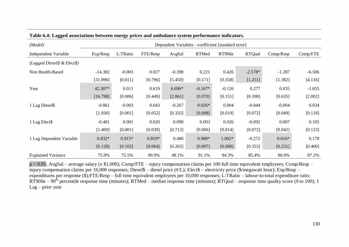
130

Table 6.4: Lagged associations between energy prices and ambulance system performance indicators.

(Model) Dependent Variables - coefficient [standard error]

Independent Variable Exp/Resp L:TRatio FTE/Resp AvgSal RTMed RT90ile RTQual Comp/Resp Comp/FTE

(Lagged Diesel$ & Elect$)

Non Health-Based -14.382

[31.896]

-0.003

[0.011]

0.027

[0.796]

-0.398

[5.450]

0.221

[0.171]

0.426

[0.358]

-2.578*

[1.251]

-1.287

[1.382]

-6.506

[4.116]

Year 42.307*

[16.798]

0.011

[0.006]

0.619

[0.449]

6.696*

[2.861]

-0.167*

[0.070]

-0.126

[0.151]

0.277

[0.398]

0.035

[0.635]

-1.655

[2.002]

1 Lag Diesel$ -0.861

[1.930]

-0.003

[0.001]

0.043

[0.052]

-0.267

[0.332]

0.026*

[0.008]

0.004

[0.019]

-0.044

[0.072]

-0.004

[0.049]

0.034

[0.118]

1 Lag Elect$ -0.481

[1.469]

0.001

[0.001]

0.020

[0.039]

0.098

[0.713]

0.003

[0.006]

0.026

[0.014]

-0.092

[0.072]

0.007

[0.042]

0.105

[0.123]

1 Lag Dependent Variable 0.832*

[0.128]

0.915*

[0.102]

0.819*

[0.064]

0.480

[0.265]

0.980*

[0.097]

1.002*

[0.068]

-0.272

[0.353]

0.616*

[0.231]

0.178

[0.400]

Explained Variance 75.9% 75.5% 90.9% 48.1% 91.1% 94.3% 85.4% 86.0% 87.2%

p < 0.05; AvgSal – average salary (x $1,000); Comp/FTE – injury compensation claims per 100 full time equivalent employees; Comp/Resp –

injury compensation claims per 10,000 responses; Diesel$ – diesel price (¢/L); Elect$ – electricity price ($/megawatt hour); Exp/Resp –

expenditures per response ($);FTE/Resp – full time equivalent employees per 10,000 responses; L:TRatio – labour-to-total expenditure ratio;

RT90ile – 90th percentile response time (minutes); RTMed – median response time (minutes); RTQual – response time quality score (0 to 100); 1

Lag – prior year

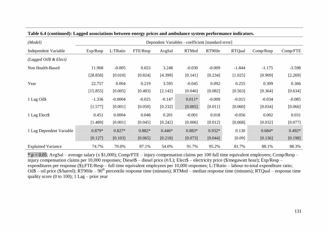
131

Table 6.4 (continued): Lagged associations between energy prices and ambulance system performance indicators.

(Model) Dependent Variables - coefficient [standard error]

Independent Variable Exp/Resp L:TRatio FTE/Resp AvgSal RTMed RT90ile RTQual Comp/Resp Comp/FTE

(Lagged Oil$ & Elect)

Non Health-Based 11.968

[28.858]

-0.005

[0.010]

0.653

[0.824]

3.248

[4.399]

-0.030

[0.141]

-0.009

[0.234]

-1.844

[1.025]

-1.175

[0.909]

-3.598

[2.269]

Year 22.757

[15.855]

0.004

[0.005]

0.219

[0.483]

3.595

[2.142]

-0.045

[0.046]

0.092

[0.082]

0.255

[0.563]

0.309

[0.364]

0.366

[0.634]

1 Lag Oil$ -1.336

[1.577]

-0.0004

[0.001]

-0.025

[0.050]

-0.147

[0.232]

0.011*

[0.005]

-0.009

[0.011]

-0.015

[0.060]

-0.034

[0.034]

-0.085

[0.066]

1 Lag Elect$ 0.451

[1.489]

0.0004

[0.001]

0.048

[0.045]

0.201

[0.242]

-0.001

[0.006]

0.018

[0.012]

-0.056

[0.068]

0.002

[0.032]

0.031

[0.077]

1 Lag Dependent Variable 0.879*

[0.127]

0.827*

[0.103]

0.882*

[0.065]

0.446*

[0.218]

0.883*

[0.073]

0.932*

[0.044]

0.130

[0.09]

0.684*

[0.136]

0.492*

[0.198]

Explained Variance 74.7% 70.0% 87.1% 54.0% 91.7% 95.2% 81.7% 88.1% 88.3%

* p < 0.05; AvgSal – average salary (x $1,000); Comp/FTE – injury compensation claims per 100 full time equivalent employees; Comp/Resp –

injury compensation claims per 10,000 responses; Diesel$ – diesel price (¢/L); Elect$ – electricity price ($/megawatt hour); Exp/Resp –

expenditures per response ($);FTE/Resp – full time equivalent employees per 10,000 responses; L:TRatio – labour-to-total expenditure ratio;

Oil$ – oil price ($/barrel); RT90ile – 90th percentile response time (minutes); RTMed – median response time (minutes); RTQual – response time

quality score (0 to 100); 1 Lag – prior year

132

6.5.4 Results for Systems without Electricity Data

Table 6.5 shows the results for the GEE modelling limited to the WA and NT

data, for which electricity price data were not available. The labour-to-total expenditure

ratio increased over time in all of the models. The 90th percentile response time

increased over time in the contemporaneous models of both diesel price and oil price.

Median response time increased over time in the lagged models, while response time

quality decreased over time. As in the analyses above, expenditures per response,

labour-to-total expenditure ratio, 90th percentile response time and response time quality

were all significantly associated with their prior year values in the lagged analyses.

6.5.4(a) Effects of Diesel and Oil Price in Systems without Electricity Data

The only contemporaneous effect of diesel or oil price in the systems without

electricity data was a positive association between FTE per 10,000 responses and both

diesel (0.163 [0.072]) and oil (0.072 [0.027]) prices. There was a downward effect of

increasing lagged diesel price on both expenditures per response (-4.143 [1.449]) and

labour-to-total expenditure ratio (-0.002 [0.0004]); the effect of lagged oil price on

resource indicators was limited to the labour-to-total expenditure ratio (-0.001

[0.0004]). There was also an association between response time quality score and both

lagged diesel price (0.703 [0.153]) and lagged oil price (0.410 [0.129]).

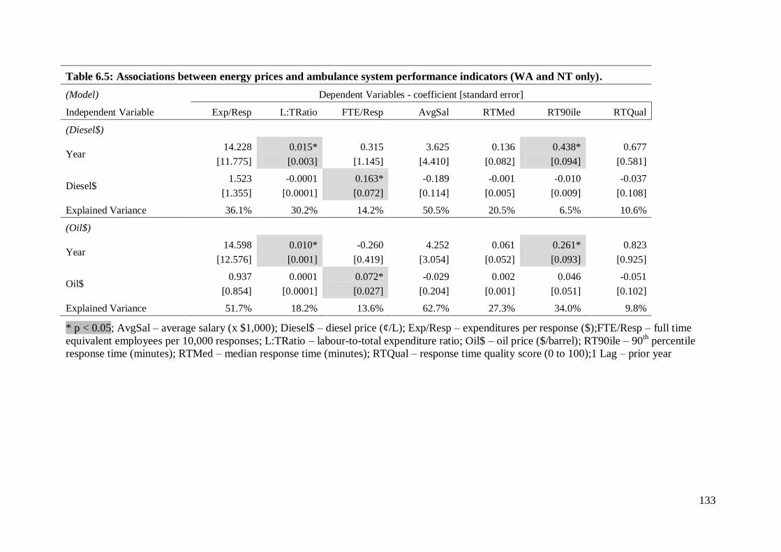
133

Table 6.5: Associations between energy prices and ambulance system performance indicators (WA and NT only).

(Model) Dependent Variables - coefficient [standard error]

Independent Variable Exp/Resp L:TRatio FTE/Resp AvgSal RTMed RT90ile RTQual

(Diesel$)

Year 14.228

[11.775]

0.015*

[0.003]

0.315

[1.145]

3.625

[4.410]

0.136

[0.082]

0.438*

[0.094]

0.677

[0.581]

Diesel$ 1.523

[1.355]

-0.0001

[0.0001]

0.163*

[0.072]

-0.189

[0.114]

-0.001

[0.005]

-0.010

[0.009]

-0.037

[0.108]

Explained Variance 36.1% 30.2% 14.2% 50.5% 20.5% 6.5% 10.6%

(Oil$)

Year 14.598

[12.576]

0.010*

[0.001]

-0.260

[0.419]

4.252

[3.054]

0.061

[0.052]

0.261*

[0.093]

0.823

[0.925]

Oil$ 0.937

[0.854]

0.0001

[0.0001]

0.072*

[0.027]

-0.029

[0.204]

0.002

[0.001]

0.046

[0.051]

-0.051

[0.102]

Explained Variance 51.7% 18.2% 13.6% 62.7% 27.3% 34.0% 9.8%

* p < 0.05; AvgSal – average salary (x $1,000); Diesel$ – diesel price (¢/L); Exp/Resp – expenditures per response ($);FTE/Resp – full time

equivalent employees per 10,000 responses; L:TRatio – labour-to-total expenditure ratio; Oil$ – oil price ($/barrel); RT90ile – 90th percentile

response time (minutes); RTMed – median response time (minutes); RTQual – response time quality score (0 to 100);1 Lag – prior year

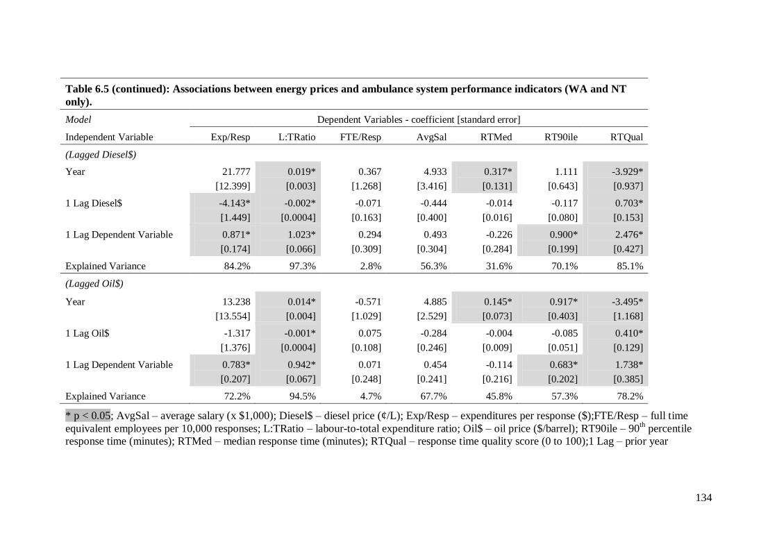
134

Table 6.5 (continued): Associations between energy prices and ambulance system performance indicators (WA and NT

only).

Model Dependent Variables - coefficient [standard error]

Independent Variable Exp/Resp L:TRatio FTE/Resp AvgSal RTMed RT90ile RTQual

(Lagged Diesel$)

Year 21.777

[12.399]

0.019*

[0.003]

0.367

[1.268]

4.933

[3.416]

0.317*

[0.131]

1.111

[0.643]

-3.929*

[0.937]

1 Lag Diesel$ -4.143*

[1.449]

-0.002*

[0.0004]

-0.071

[0.163]

-0.444

[0.400]

-0.014

[0.016]

-0.117

[0.080]

0.703*

[0.153]

1 Lag Dependent Variable 0.871*

[0.174]

1.023*

[0.066]

0.294

[0.309]

0.493

[0.304]

-0.226

[0.284]

0.900*

[0.199]

2.476*

[0.427]

Explained Variance 84.2% 97.3% 2.8% 56.3% 31.6% 70.1% 85.1%

(Lagged Oil$)

Year 13.238

[13.554]

0.014*

[0.004]

-0.571

[1.029]

4.885

[2.529]

0.145*

[0.073]

0.917*

[0.403]

-3.495*

[1.168]

1 Lag Oil$ -1.317

[1.376]

-0.001*

[0.0004]

0.075

[0.108]

-0.284

[0.246]

-0.004

[0.009]

-0.085

[0.051]

0.410*

[0.129]

1 Lag Dependent Variable 0.783*

[0.207]

0.942*

[0.067]

0.071

[0.248]

0.454

[0.241]

-0.114

[0.216]

0.683*

[0.202]

1.738*

[0.385]

Explained Variance 72.2% 94.5% 4.7% 67.7% 45.8% 57.3% 78.2%

* p < 0.05; AvgSal – average salary (x $1,000); Diesel$ – diesel price (¢/L); Exp/Resp – expenditures per response ($);FTE/Resp – full time

equivalent employees per 10,000 responses; L:TRatio – labour-to-total expenditure ratio; Oil$ – oil price ($/barrel); RT90ile – 90th percentile

response time (minutes); RTMed – median response time (minutes); RTQual – response time quality score (0 to 100);1 Lag – prior year

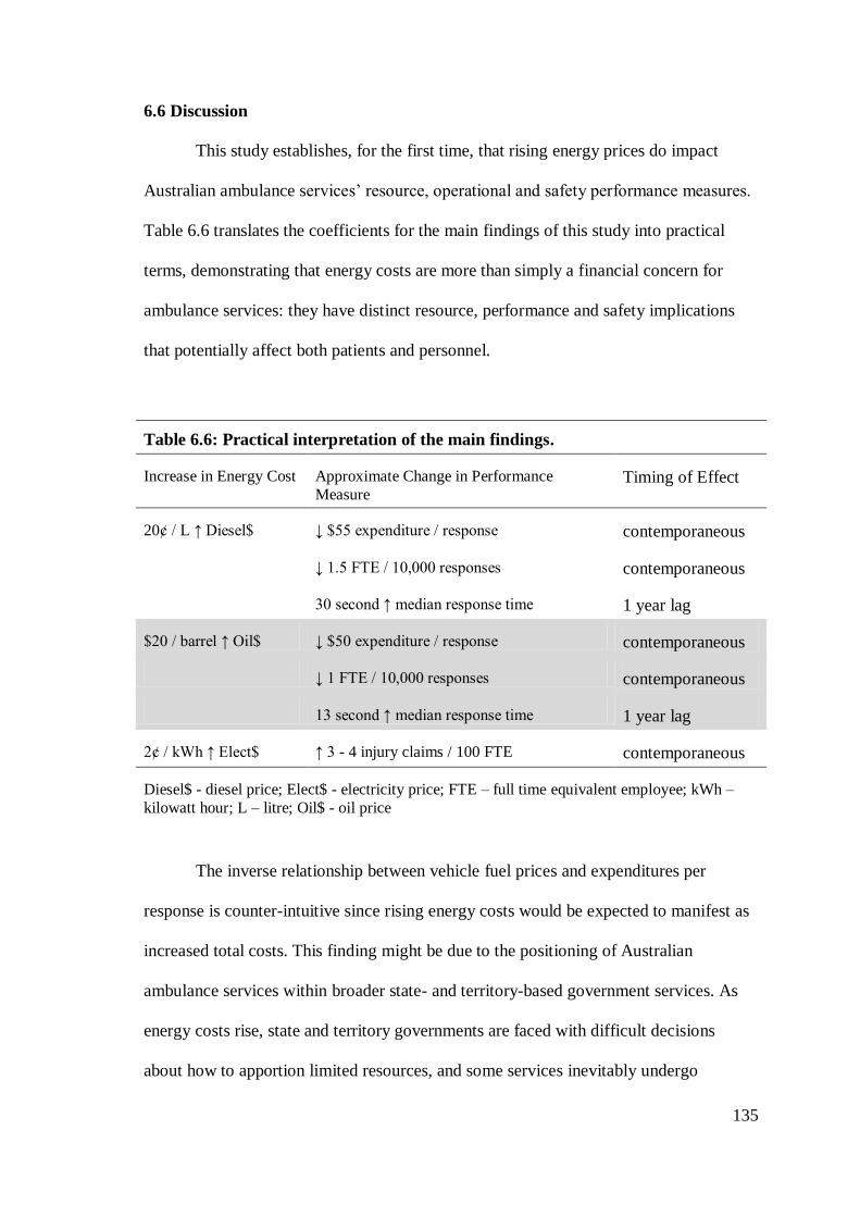
135

6.6 Discussion

This study establishes, for the first time, that rising energy prices do impact

Australian ambulance services’ resource, operational and safety performance measures.

Table 6.6 translates the coefficients for the main findings of this study into practical

terms, demonstrating that energy costs are more than simply a financial concern for

ambulance services: they have distinct resource, performance and safety implications

that potentially affect both patients and personnel.

Table 6.6: Practical interpretation of the main findings.

Increase in Energy Cost Approximate Change in Performance

Measure Timing of Effect

20¢ / L ↑ Diesel$ ↓ $55 expenditure / response contemporaneous

↓ 1.5 FTE / 10,000 responses contemporaneous

30 second ↑ median response time 1 year lag

$20 / barrel ↑ Oil$ ↓ $50 expenditure / response contemporaneous

↓ 1 FTE / 10,000 responses contemporaneous

13 second ↑ median response time 1 year lag

2¢ / kWh ↑ Elect$ ↑ 3 - 4 injury claims / 100 FTE contemporaneous

Diesel$ - diesel price; Elect$ - electricity price; FTE – full time equivalent employee; kWh –

kilowatt hour; L – litre; Oil$ - oil price

The inverse relationship between vehicle fuel prices and expenditures per

response is counter-intuitive since rising energy costs would be expected to manifest as

increased total costs. This finding might be due to the positioning of Australian

ambulance services within broader state- and territory-based government services. As

energy costs rise, state and territory governments are faced with difficult decisions

about how to apportion limited resources, and some services inevitably undergo

136

reductions in their allocations. These data suggest ambulance service budgets suffer in

times of rising fuel prices—or, conversely, that ambulance service budgets benefit when

fuel prices drop.

In this study, increases in diesel and oil prices manifested not only as reduced

expenditures per response, but also as a reduction in FTE per 10,000 responses. These

data are contrary to previous data from industry, where labour is generally a substitute

for energy (Arnberg & Bjorner, 2007; Nguyen & Streitwieser, 1999; Woodland, 1993).

While the explained variance in these models was low (13-14%) the effect sizes were

quite meaningful. For instance, an ambulance system responding to 100,000 calls per

year could lose as many as 15 FTE if the TGP for diesel increased just 20 cents per L.

Certainly ambulance systems would be unlikely to electively institute layoffs in

response to energy price rises in the short term, but they might be prevented from filling

staff vacancies that result from natural attrition or from adding additional employees

despite increasing response volumes.

Increasing electricity prices were associated with increased injury compensation

claims per 100 FTE, whether electricity price was modelled with diesel price or with oil

price. Although safety performance indicators were only available for four systems and

a small subset of the system-years represented in this study, the models for injury

compensation claims per 100 FTE were strong, with explained variances of around

80%. To my knowledge, this is the first evaluation to report a link between rising

energy prices and increasing workplace injury claims. A 2007 investment analysis of

Australian companies reported an association between lower scores in workplace health

and safety indices and lower returns in the share market, but that analysis did not

explore the role of energy costs (if any) in that relationship (Gray, 2007). There are a

number of theoretical mechanisms that might explain this finding. For example,

137

ambulance service employees would individually face the same increases in energy

prices, and they might choose to work additional overtime shifts or take on second jobs

to bolster their household budgets. Extra work hours—whether in their primary job or a

second job—could lead to worker fatigue, which is associated with increased risk of

workplace injury and fatality among ambulance personnel (Maguire 2011; Maguire,

Hunting, Smith, & Levick, 2002; Patterson et al., 2012; Studnek & Fernandez, 2008).

Finally, increasing diesel price was associated with an increase in median

response time in the following year, and the same positive association between fuel

prices and median response time was seen when modelling lagged oil price instead of

lagged diesel price. While there are very few emergencies for which an association

between rapid ambulance response and decreased mortality has been demonstrated

(Blackwell & Kaufman, 2002; Blanchard et al., 2012; De Maio, Stiell, Wells, & Spaite,

2003; Pons et al., 2005; Pons & Markovchick, 2002), most ambulance systems are still

expected to meet rigid response time standards. This requires considerable resources in

the form of vehicles, stations, and personnel. This study now provides empirical data

supporting the intuitive notion that the erosion of ambulance service resources by

increasing energy prices eventually results in delayed ambulance response times.

6.7 Limitations and Future Studies

One limitation of this study is that diesel price data were only available for the

most recent six year period, so world crude oil price was included as an indirect

measure of vehicle fuel costs. However, despite the different time spans for which the

diesel and oil price data were available, little variation in the results was observed when

modelling the effects of the two energy sources. The coefficients, the significance of the

findings, and the explained variances in the models were nearly identical for the

138

analyses of diesel and electricity prices compared with those for oil and electricity

prices. While adding the oil price data to the analyses did not meaningfully alter the

outcome, this was not wasted effort; the consistency of the results adds to the

confidence in the findings.

Another potential limitation is that this analysis depends on summary data

extracted from annual reports of the ambulance agencies or their parent organisations,

rather than data specifically collected for this study. Also, data for ambulance-related

activities that are not delivered by the states and territories, most notably the Royal

Flying Doctor Service but also other small independent agencies, are not included in

this analysis. These are, however, non-differential information biases that would result

in bias towards the null hypothesis.

That complete electricity price data were not available for all states and

territories is another limitation of this study. The results of the separate analyses of the

data for the two jurisdictions without electricity price data do differ from those of the

main analyses, but they do not contradict the main findings. In fact, although it was a

lagged rather than contemporaneous effect, increasing diesel and oil prices were

associated with decreased resource allocation in those two ambulance systems as well.

Lastly, these are aggregate-level ecological data (in the epidemiologic sense) on

an annual scale; they cannot be extrapolated to individual ambulance responses, or to

shorter-run (for example, weekly or monthly) changes in energy prices.

Future studies might seek to explain the exact mechanisms of the effects

observed in this study. Ambulance services involve vehicles, equipment, buildings,

communication systems, and personnel, as well as information technology systems,

clinical training activities, physician oversight, and administrative structures (Lerner,

Nichol, Spaite, Garrison, & Maio, 2007). Fluctuating energy prices could conceivably

139

impact any or all of these inter-related components. It is also possible that ambulance

services are able to achieve efficiencies in the face of rising energy prices so that the

resource, operational and safety insults identified in this study do not diminish patient

care, but further study is needed to explicitly explore the effects of rising energy costs

on patient outcomes. The effects of energy costs on ambulance systems in other

countries, particularly those where ambulance services operate as free-market

enterprises, also remain to be determined. More broadly, the impact of energy scarcity

and rising prices on other aspects of the health care system is an area in need of

substantial research.

6.8 Conclusion

This study was undertaken to empirically evaluate the impact of energy price

fluctuations on ambulance services. The main finding of this analysis is that the null

hypothesis is rejected: there is an association between energy prices and Australian

ambulance service resource, operational and safety performance characteristics. Diesel

prices and oil prices have a contemporaneous inverse relationship with expenditures per

response and FTE per 10,000 responses in most states, and a lagged inverse relationship

with resource measures in other states; that is, higher energy prices are associated with

diminished resource allocation. There is also a one-year lagged association between

increasing diesel and oil prices and increasing median ambulance response times.

Finally, there is a contemporaneous association between higher electricity prices and

increasing injury compensation claims that is seen whether electricity price is modelled

simultaneously with diesel price or oil price.

140

Chapter 7: Summary Discussion and Concluding Remarks

The previous four chapters have reviewed the literature related to health-related

emissions, described the Scope 1 and Scope 2 greenhouse gas emissions of Australian

ambulance operations, estimated their complete life cycle emissions, and demonstrated

that their energy consumption is not only an environmental issue, but also an economic

concern. This chapter summarises the key findings of this thesis, discusses their

relevance to Australian ambulance systems, and provides some suggestions for future

research.

Portions of this chapter (sections 7.3 and 7.4) have been partially adapted from

the manuscript: Brown, L.H., Blanchard, I.E. (2012). Energy, emissions, and emergency

medical services: Policy matters. Energy Policy, 46, 585-593. The published version of

the paper is reproduced in Appendix 3.

141

7.1 Summary of Findings

7.1.1 Health Systems Emissions

The greenhouse gas emissions of health systems and health related activities are

not widely studied; the literature review identified only 32 studies explicitly evaluating

the energy consumption or environmental impacts of health services. What is known

from the literature is that on a per-event or per-patient basis, health related emissions are

small, usually measured on the order of tens or hundreds of kg CO2e per patient. In the

aggregate, however, health sector emissions are substantial, representing 3% of total

greenhouse gas emissions in England (Sustainable Development Commission-

Stockholm Environment Institute, 2008) and 8% of total emissions in the U.S. (Chung

& Meltzer, 2009).

Prior to this thesis, the only published works on EMS-related emissions were

from North America, where Scope 1 and Scope 2 emissions were estimated to average

45.5 kg CO2e per ambulance response. Vehicle fuels accounted for 72% of emissions

from ground EMS operations in North America, with electricity consumption

responsible for 20% of emissions and other fuels making up the remainder. For the

U.S., annual emissions from ground EMS activities were estimated at 660,000 to 1.6

million t CO2e. Emissions from air medical activities were much greater than for ground

EMS activities, estimated at approximately 1 t CO2e per air ambulance mission

(Blanchard & Brown, 2011).

7.1.2 Scope 1 and Scope 2 Emissions from Australian Ambulance Services

The Scope 1 and 2 emissions from Australian ambulance operations compare

favourably to those of North American EMS systems; for ground ambulance operations

they are estimated at 22 kg CO2e per response. In the aggregate, Australian state and

142

territory based ambulance services are estimated to emit approximately 110,000 to

120,000 t of Scope 1 and Scope 2 greenhouse gases each year. While this represents a

small proportion of total Australian emissions, it is of the same order as other important

subsectors of the Australian economy.

Interestingly, electricity consumption is responsible for a larger share of

Australian ground ambulance services’ Scope 1 and Scope 2 emissions when compared

with North America: approximately 41% vs. 20%. Also, on a per-patient basis,

emissions from Australian air ambulance services are approximately five times those of

North American air ambulance services.

7.1.3 Complete Life Cycle Emissions of Australian Ambulance Services

The complete life cycle emissions of Australian ambulance services are

estimated to total between approximately 216,000 and 547,000 t CO2e per year. While

this seems a large range, it provides a useful—if inexact—indication of the scale of

EMS related emissions in Australia. They represent between 1.8% and 4.4% of all

Australian health sector emissions. As ambulance-related expenditures represent 1.7%

of total health sector expenditures, ambulance services are likely responsible for a

disproportionate share of health sector emissions, and thus might be able to play a

meaningful role in efforts to reduce health sector emissions.

Scope 1 emissions represent approximately 20% of complete life cycle

emissions from Australian ambulance systems, with Scope 2 electricity consumption

responsible for 22% of emissions and upstream Scope 3 emissions accounting for 58%.

Depending on whether the economic structures of Australian ambulance systems more

closely resemble the remainder of the ‘health services’ sector, the ‘other services’ sector

(which includes police and fire services), or the ‘government services’ sector, the

143

leading structural paths contributing to their complete life cycle emissions would

include such intuitive and counter-intuitive things as: basic chemicals; wholesale trade;

gas production and distribution; lime; sheep and shorn wool; beef cattle for meat

products; air and space transport; pulp, paper and paperboard; and softwoods for pulp,

paper and paperboard (Foran, Lenzen, & Dey, 2005).

7.1.4 Energy Costs and Australian Ambulance Systems

Environmental concerns are not the only reason for Australian ambulance

systems to evaluate and manage their energy consumption. Energy costs have a

demonstrable impact on Australian ambulance services. A 20 cent per L increase in

diesel price is associated with a $55 per ambulance response decrease in ambulance

service expenditures; it is also associated with a staffing decrease of 1.5 FTE per 10,000

responses. In the year following a 20 cent per L increase in diesel price, median

response times increase by 30 seconds. A 2 cent per kWh increase in electricity price is

associated with an increase of three to four injury claims per 100 FTE annually.

While the mechanisms by which these effects occur remain to be determined,

they do indicate that rising energy costs can adversely affect ambulance operations in

ways that potentially impact both patients and ambulance service personnel. In this

research, the influence of energy costs was measured only in the short run—that is, in

the same year or first year after the price changes occurred. The long-run effects of

energy prices on ambulance services, as well as the effects of persistent price increases

(as opposed to price fluctuations), remain to be determined.

144

7.2 Relevance of the Findings

What do Australian ambulance operations take from this research? How can

these data be used to foster the sustainability of Australian emergency ambulance

operations?

First, while these data demonstrate that ambulance services are not, on a national

scale, ‘big emitters’, they do produce a meaningful amount of greenhouse gas

emissions. Policy efforts to constrain greenhouse gas emissions will affect Australian

ambulance systems.

Second, in terms of the Scope 1 and Scope 2 emissions most easily influenced

by EMS systems, consumption of vehicle fuels is the primary contributor to the carbon

footprint of Australian ambulance systems, but electricity consumption is also

responsible for a substantial portion their emissions. Efforts to minimise the carbon

footprint of Australian ambulance services and ensure their environmental sustainability

should target both of these energy sources.

Third, the direct emissions from air ambulance transport are approximately 200

times those of ground ambulance transport. Optimising the use of air medical resources

is another potential strategy for reducing ambulance system emissions and energy

consumption.

Fourth, the complete life cycle emissions of Australian ambulance services,

including the upstream emissions from products and services in the supply chain, total

approximately 216,000 to 547,000 t CO2e each year, and account for between 1.8% and

4.4% of total Australian health sector emissions. This means ambulance services could

make a meaningful contribution in efforts to reduce health sector emissions—which

could be both an opportunity and a threat.

145

Fifth, around 60% of ambulance service complete life cycle emissions arise

from upstream, Scope 3, processes. Implementing environmentally friendly purchasing

practices would be required to achieve substantial reductions in the complete life cycle

emissions of ambulance services. The upstream products and services that contribute

most to the complete life cycle emissions of ambulance services include some products

and services that are not intuitively linked to ambulance services. Advocating for green

electricity generation, which could reduce emissions at all stages of the supply chain, is

one way ambulance systems could reduce their complete life cycle emissions.

Sixth, energy consumption is not only an environmental issue for Australian

ambulance systems. Energy costs have measurable effects on ambulance service

resource, operational, and safety measures that could impact both patient care and

employee well-being. Managing greenhouse gas emissions is managing energy

consumption, and vice-versa. That is, there are both environmental and economic

aspects to the ‘sustainability’ of Australian ambulance operations.

7.3 Strategies for Reducing the Energy and Environmental Burden of Ambulance

Services

There are a number of strategies that ambulance agencies could adopt to reduce

their energy consumption and greenhouse gas emissions and facilitate their adaptation

to a low(er) carbon economy. Generally these can be described in the context of the

‘IPAT’ equation. While the IPAT equation primarily describes functions on an

economy-wide level, the principles can also be applied to economic subsectors or

individual enterprises (Waggoner & Ausubel, 2002; York, Rosa, & Dietz, 2003). That

is, ambulance services can reduce their environmental impact (‘I’) by addressing the

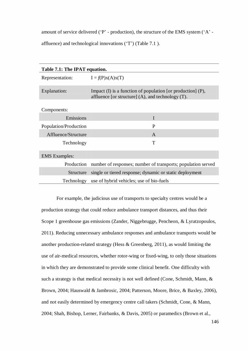
146

amount of service delivered (‘P’ - production), the structure of the EMS system (‘A’ -

affluence) and technological innovations (‘T’) (Table 7.1 ).

Table 7.1: The IPAT equation.

Representation: I = f(P)x(A)x(T)

Explanation: Impact (I) is a function of population [or production] (P),

affluence [or structure] (A), and technology (T).

Components:

Emissions I

Population/Production P

Affluence/Structure A

Technology T

EMS Examples:

Production number of responses; number of transports; population served

Structure single or tiered response; dynamic or static deployment

Technology use of hybrid vehicles; use of bio-fuels

For example, the judicious use of transports to specialty centres would be a

production strategy that could reduce ambulance transport distances, and thus their

Scope 1 greenhouse gas emissions (Zander, Niggebrugge, Pencheon, & Lyratzopoulos,

2011). Reducing unnecessary ambulance responses and ambulance transports would be

another production-related strategy (Hess & Greenberg, 2011), as would limiting the

use of air-medical resources, whether rotor-wing or fixed-wing, to only those situations

in which they are demonstrated to provide some clinical benefit. One difficulty with

such a strategy is that medical necessity is not well defined (Cone, Schmidt, Mann, &

Brown, 2004; Hauswald & Jambrosic, 2004; Patterson, Moore, Brice, & Baxley, 2006),

and not easily determined by emergency centre call takers (Schmidt, Cone, & Mann,

2004; Shah, Bishop, Lerner, Fairbanks, & Davis, 2005) or paramedics (Brown et al.,

147

2009; Snooks, Dale, Hartley-Sharpe, & Halter, 2004). Further, in most developed

countries there is a societal expectation of service on demand that would need to be

addressed. Also, particularly in Australia, some emergency responses and transports

require air-medical resources for logistical reasons, independent of patient condition.

Health promotion and injury/illness prevention initiatives, such as those

targeting heart disease and motor vehicle crashes, would be indirect production-related

strategies with the dual benefits of improved public health and reduced demand for

ambulance transport.

An example of a structure-related strategy would be to change the way

ambulance systems respond to emergency calls. Presently, most EMS systems must

meet rigid response time standards for all unscheduled calls (Bailey & Sweeney, 2003;

Myers et al., 2008)—which requires considerable resources in the form of vehicles,

stations, and personnel—even though there are very few emergencies for which an

association between rapid EMS response and decreased morbidity or mortality has been

demonstrated (Blackwell & Kaufman, 2002; Blanchard et al., 2012; De Maio, Stiell,

Wells, & Spaite, 2003; Pons et al., 2005; Pons & Markovchick, 2002). Response time

policies that support responding to individual situations in the optimal amount of time,

instead of all situations in a uniformly short amount of time, could reduce EMS system

resource requirements (Eisenberg, Bergner, & Hallstrom, 1979) and thus energy

consumption and emissions. Reducing driving speeds when transporting stable patients

without life-threatening conditions to hospital might also reduce energy consumption

and emissions. Driving ambulances with the flow of traffic, without warning lights and

sirens, only marginally increases ambulance transport times (Brown, Whitney, Hunt,

Addario, & Hogue, 2000; Hunt et al., 1995).

148

Another strategy would be reduced ambulance idling at emergency scenes and

hospitals. Many EMS agencies are reluctant to shut down ambulances at emergency

scenes, as the ambulance warning lights provide some measure of safety. Reducing

idling at receiving hospitals, however, might be effective in reducing energy

consumption and emissions given the extended off-load times confronting many EMS

systems as a result of emergency department overcrowding (Eckstein et al., 2005;

Vandeventer et al., 2011). A structural aspect of ambulance systems in particular need

of research is the relative energy consumption and emissions profiles of fixed-station

versus dynamic deployment staging strategies (the two predominant types of

deployment strategy used in EMS). A fixed-station strategy has the added energy

burden of stationhouses and usually longer response distances; a dynamic deployment

strategy has the added fuel consumption of ambulances being constantly relocated to

street-corner posts in order to minimise response distances and response times.

As thoroughly discussed in Chapter 5, technology-related strategies would

include the use of hydrogen FCV ambulances (Burtt, 2008) and/or electric or hybrid

vehicles for administrative and support vehicle fleets (Hawkins, 2008). However, while

hydrogen FCV and electric vehicles have lower tailpipe emissions, their true

environmental impact ultimately depends on local electricity generation processes

(Leaver & Gillingham 2010; McCarthy & Yang, 2010; Ozalp, Epstein, & Kogan, 2010;

Perujo & Ciuffo, 2010; Pro, Hammerschlag, & Mazza, 2005; Sioshansi, Fagiani, &

Marano, 2010; Vergragt & Brown, 2007). Similarly, the use of bio-diesel would be a

technology related strategy, but as with hydrogen FCV and electric vehicles, bio-fuels

are not universally carbon-neutral (Searchinger et al., 2008; Solomon, 2010), and

availability of sufficient quantities, particularly in rural areas, might also be a limitation

on such a strategy.

149

Expanded utilisation of telemedicine is a technology-related strategy that might

also be able to reduce the need to transport some patients (Patterson, 2005; Smith et al.,

2007; Smith, Patterson, & Scott, 2007; Yellowlees, Chorba, Parish, Wynn-Jones, &

Nafiz, 2010). Finally, using electronic (rather than paper) forms for medical records and

research activities can also reduce the environmental burden of health services,

including ambulance services (Chakladar, Eckstein, & White, 2011; Turley et al., 2011).

There are certainly other potential strategies for reducing ambulance-related

energy consumption and emissions. Importantly, however, none of these proposed

strategies have been empirically evaluated; their actual impact on energy consumption,

emissions and patient outcomes, as well as their social acceptability, remain to be

determined.

7.4 Directions for the Future

A number of questions remain to be answered: What efforts are Australian

ambulance services already undertaking to reduce their greenhouse gas emissions?

What barriers do those efforts face? How effective are those strategies? Future research

could also attempt an inventory based assessment of the complete life cycle emissions

of Australian ambulance services, allowing a more specific evaluation of the structural

paths contributing to those emissions.

Also, while this thesis focuses on Australian ambulance services, these are

international issues. What are the Scope 1, Scope 2 and complete life cycle emissions of

ambulance services in other countries? How do they compare with those of Australian

and North American EMS systems? Are there specific ambulance system characteristics

that are associated with higher or lower emissions profiles? Are the energy and

150

environmental issues for EMS systems representative of, and instructive for, other

aspects of the health system?

Finally, the specific strategies discussed in Section 7.3 above—and any other

proposed strategies—will require evaluation. For example: Does accelerating a fleet

replacement schedule, replacing older low-efficiency vehicles with modern high-

efficiency vehicles, significantly reduce Scope 1 emissions? What effect does such a

strategy have on complete life cycle emissions? Do ambulance services with flexible

response time requirements have lower emissions profiles than those with shorter, more

stringent response time standards?

There is much more to be done. Some of these future studies are already

underway; some are being planned; some will have to be left to others to complete. As I

wrote at the beginning of this thesis, “This is the commencement—not the

culmination—of an effort to ensure the sustainability of EMS systems”. The conclusion

of this thesis is not the resolution of this issue, and it is not the end of my research in

this area.

Another door has opened....

151

Bibliography

Adelman, M.A. (2002). World oil production & prices 1947-2000. Quarterly Review of

Economics and Finance, 42, 169-191.

Agar, J.W.M. (2010). Conserving water in and applying solar power to haemodialysis:

‘Green Dialysis’ through wise resource utilization. Nephrology, 15, 448-453.

Agar, J.W.M., Simmonds, R.E., Knight, R., Somerville, C.A. (2009). Using water

wisely: New, affordable, and essential water conservation practices for facility and

home hemodialysis. Hemodialysis International, 13, 32-37.

Aleklett, K., Hook, M., Jakobsson, K., Lardelli, M., Snowden, S., Soderbergh, B.

(2010). The peak of the oil age – Analyzing the world oil production Reference

Scenario in World Energy Outlook 2008. Energy Policy, 38, 1398-1414.

Allen, M.R., Frame, D.J., Huntingford, C., Jones, C.D., Lowe, J.A., Meinshausen, M.,

Meinshausen, N. (2009). Warming caused by cumulative carbon emissions towards the

trillionth tonne. Nature, 458, 1163-1166.

Anonymous. (2008). Practices urged to lighten carbon footprint. British Dental Journal,

204(9), 483.

Anonymous. (2010). Trust takes strides in cutting carbon footprint. Nursing Standard,

24(40), 6.

Anonymous. (2011). Ambulance service’s budget pressure over diesel price. BBC News

(17 February). Retrieved from: www.bbc.co.uk on 18 February 2011.

Armstrong, R. (2009). Government 3% cuts begin to bite. W.A. Police News. October

Issue, 4.

152

Arnberg, S., Bjorner, T.B. (2007). Substitution between energy, capital and labour

within industrial companies: A micro panel data analysis. Resource and Energy

Economics, 29, 122-136.

Associated Press. (2008). Pumps still dry in western N.C. The [Greensboro, NC] News-

Record. Retrieved from: www.news-record.com on 09 July 2009.

Australian Bureau of Statistics. (2006). Australian and New Zealand Standard

Industrial Classification 2006 (ANZSIC). Canberra, ACT: Commonwealth of Australia.

Australian Bureau of Statistics. (2011). National Statistics. Retrieved from:

www.abs.gov.au on 18 July 2011.

Australian Bureau of Statistics. (2012). Consumer Price Index, Australia, Dec 2011.

Canberra, ACT: Commonwealth of Australia. Retrieved from: www.abs.gov.au on 27

January 2012.

Australian Energy Market Operator. (2010). Average Price Tables. Retrieved from:

www.aemo.com.au on 24 May 2011.

Australian Government Department of Climate Change. (2009a). National Greenhouse

and Energy Reporting Streamlining Protocol. Canberra: Commonwealth of Australia.

Australian Government Department of Climate Change. (2009b). Australia’s National

Greenhouse Accounts. Canberra, ACT: Commonwealth of Australia.

Australian Government Department of Climate Change. (2009c). National Greenhouse

Accounts (NGA) Factors. Canberra: Commonwealth of Australia.

153

Australian Institute of Health and Welfare. (2011). Spending on health exceeds $120

billion. Canberra, ACT: Commonwealth of Australia. Retrieved from:

www.aihw.gov.au on 30 January 2012.

Australian Institute of Petroleum. (2010). Terminal Gate Prices (TGPs): Historical

Averages for Petrol and Diesel. Retrieved from: www.aip.com.au/pricing/tgp.htm on 24

May 2011.

Australian Tax Office. (2011). Foreign Exchange Rates. Retrieved from:

www.ato.gov.au on 25 May 2011.

Baboulet, O., Lenzen, M. (2010). Evaluating the environmental performance of a

university. Journal of Cleaner Production, 18, 1134-1141.

Bagliani, M., Galli, A., Niccolucci, V., Marchettini, N. (2008). Ecological footprint

analysis applied to a sub-national area: The case of the Province of Siena (Italy).

Journal of Environmental Management, 86, 354-364.

Bailey, D.M. (1980). Energy contingency planning for health facilities: Conference

report. Public Health Reports, 95, 58-61.

Bailey, E.D., Sweeney, T. (2003). Considerations in establishing emergency medical

services response time goals. Prehospital Emergency Care, 7, 397-399.

Bailey, J.A., Amyotte, P., Khan, F.I. (2010). Agricultural application of life cycle

iNdeX (LInX) for effective decision making. Journal of Cleaner Production, 18, 1703-

1713.

Bain, E. (2009). Environmental health 101: Your carbon footprint. Massachusetts

Nurse, 80(2), 11.

154

Baptista, P., Ribau, J., Bravo, J., Silva, C., Adcock, P., Kells, A. (2011). Fuel cell hybrid

taxi life cycle analysis. Energy Policy, 39, 4683-4691.

Barnola, J.M., Raynaud, D., Korotkevich, Y.S., Lorius, C. (1987). Vostok ice core

provides 160,000-year record of atmospheric CO2. Nature, 329, 408-414.

Bayazit, Y., Sparrow, E.M. (2010). Energy efficiency comparison of forced-air versus

resistance heating devices for perioperative hypothermia management. Energy, 35,

1211-1215.

Beer, T., Grant, T. (2007). Life-cycle analysis of emissions from fuel ethanol and blends

in Australian heavy and light vehicles. Journal of Cleaner Production, 15, 833-837.

Bera, P.P., Francisco, J.S., Lee, T.J. (2009). Identifying the molecular origin of global

warming. Journal of Physical Chemistry A, 113(45), 12694-12699.

Bicknell, K.B., Ball, R.J., Cullen, R., Bigsby, H.R. (1998). New methodology for the

ecological footprint with an application to the New Zealand economy. Ecological

Economics, 27, 149-160.

Bizzarri, G., Morini, G.L. (2004). Greenhouse gas reduction and primary energy

savings via adoption of a fuel cell hybrid plant in a hospital. Applied Thermal

Engineering, 24, 383-400.

Bizzarri, G., Morini, G.L. (2006). New technologies for an effective energy retrofit of

hospitals. Applied Thermal Engineering, 26, 161-169.

Blackwell, T.H., Kaufman, J.S. (2002). Response time effectiveness: Comparison of

response time and survival in an urban emergency medical services system. Academic

Emergency Medicine, 9, 288-295.

155

Blakemore, S. (2009). Nurses urged to take a lead in reducing the NHS carbon

footprint. Nursing Standard, 23(22), 12-13.

Blanchard, I., Brown, L.H. (2009). Carbon footprinting of EMS systems: Proof of

concept. Prehospital Emergency Care, 13, 546-549.

Blanchard, I.E., Brown, L.H. (2011). Carbon footprinting of North American

emergency medical services systems. Prehospital Emergency Care, 15, 23-29.

Blanchard, I.E., Doig, C.J., Hagel, B.E., Anton, A.R., Zygun, D.A., Kortbeek, J.B.,

Powell, D.G., Williamson, T.S., Fick, G.H., Innes, G.D. (2012). Emergency medical

services response time and mortality in an urban setting. Prehospital Emergency Care,

16, 142-151.

Booth, M. (2010). Colorado Springs cuts into services considered basic by many. The

Denver [Colorado] Post. 31 January.

Brockway, P. (2010). Carbon footprinting project evaluated. International Federation of

Hospital Engineering Digest, 07 February 2010, 1-4.

Brown, L.H., Blanchard, I.E. (2012). Energy, emissions and emergency medical

services: Policy matters. Energy Policy, 46, 585-593.

Brown, L.H., Canyon. D.V., Buettner, P.G. (In Press). The energy burden and

environmental impact of health services: A review. American Journal of Public Health.

Brown, L.H., Canyon. D.V., Buettner. P.G., Crawford. J.M., Judd. J., on behalf of the

Australian Ambulance Emissions Study Group. (In Press). The carbon footprint of

Australian ambulance operations. Emergency Medicine Australasia.

156

Brown, L.H., Devine, S. (2008). EMS & health promotion: A next step in the

collaboration between EMS and public health. Emergency Medical Services, 37(10),

109-113.

Brown, L.H., Hubble, M.W., Cone, D.C., Millin, M.G., Schwartz, B., Patterson, P.D.,

Greenberg, B., Richards, M.E. (2009). Paramedic determinations of medical necessity:

A meta analysis. Prehospital Emergency Care, 13, 516-527.

Brown, L.H., Whitney, C.L., Hunt, R.C., Addario, M., Hogue, T. (2000). Do lights and

sirens reduce ambulance response times? Prehospital Emergency Care, 4, 70-74.

Bujak, J. (2010). Heat consumption for preparing domestic hot water in hospitals.

Energy and Buildings, 42, 1047-1055.

Burnett, J. Clarke, M., Darbyshire, J., Haines, A., Lilford, R., Ramos, M., Roberts, I.,

Shakur, H., Siegfried, N., Wilkinson, P. (2007). Towards sustainable clinical trials.

British Medical Journal, 334, 671-673.

Burton, P., Gurrin, L., Sly, P. (1998). Extending the simple linear regression model to

account for correlated responses: An introduction to generalized estimating equations

and multi-level mixed modelling. Statistics in Medicine, 17, 1261-1291.

Burtt, B. (2008). Ontario ambulances go green with hydrogen systems. EMS

Responder.com. Retrieved from: www.publicsafety.com/article/article.jsp?id=4254&

siteSection=8 on 25 April 2008.

Butler, C.D. (2010). Lightening our carbon footprint: Economics, norms and doctors.

Medical Journal of Australia, 192(9), 485-486.

157

Cadarso, M-A., Lopez, L-A., Gomez, N., Tobarra, M-A. (2010). CO2 emissions of

international freight transport and offshoring: Measurement and allocation. Ecological

Economics, 69, 1682-1694.

Callister, M.E.J., Griffiths, M.J.D. (2007). The carbon footprint of the America

Thoracic Society meeting. American Journal of Respiratory and Critical Care

Medicine, 175(4), 417.

Canadian News Wire. (2009). Provincial governments cut funds for HIV/AIDS services

on World AIDS Day. December 1, 2009. Retrieved from:

www.cancelthecuts.org/node/17 on 24 February 2010.

Carnegie Mellon University Green Design Institute. (2010a). Economic Input-Output

Life Cycle Assessment (EIO-LCA), US 1997 Industry Benchmark model [Internet].

Retrieved from: www.eiolca.net on 15 December 2010.

Carnegie Mellon University Green Design Institute. (2010b). Economic Input-Output

Life Cycle Assessment (EIO-LCA), US 2002 Purchaser Price model [Internet].

Retrieved from: www.eiolca.net on 15 December 2010.

Chakladar, A., Eckstein, S., White, S.M. (2011). Paper use in ethics applications and

study conduct. Clinical Medicine, 11, 44-47.

Chirarattananon, S., Chaiwiwatworakul, P., Hien, V.D., Rakkwamsuk, P., Kubaha, K.

(2010). Assessment of energy savings from the revised building energy code of

Thailand. Energy, 35, 1741-1753.

Chung, J.W., Meltzer, D.O. (2009). Estimate of the carbon footprint of the US health

care sector. JAMA, 302, 1970-1972.

158

Clark, G.B., Kline, B. (1981). Impact of oil shortage on plastic medical supplies. Public

Health Reports, 96, 111-115.

Cone, D.C., Schmidt, T.A., Mann, N.C., Brown, L. (2004). Developing research criteria

to define medical necessity in emergency medical services. Prehospital Emergency

Care, 8, 116-125.

Connor, A., Mortimer, F. (2010). The green nephrology survey of sustainability in renal

units in England, Scottland and Wales. Journal of Renal Care, 36(3), 153-160.

Coontz, R. (2007). Wedging sustainability into public consciousness. Science, 315,

1068-1069.

Coronada, C.R., de Carvalho, J.A., Sliveira, J.L. (2009). Biodiesel CO2 emissions: A

comparison with the main fuels in the Brazilian market. Fuel Processing Technology,

90, 204-211.

Council of Ambulance Authorities. (2010). 2009-2010 Annual Report. Findon, SA: The

Council of Ambulance Authorities Inc. Retrieved from: www.caa.net.au on 26 May

2011.

Crane, J., Caldwell, B. (2006). Another inconvenient truth? British Medical Journal,

333, 1256.

Creagh, H. (2008). NHS sets up unit to encourage energy efficiency and cut carbon

emissions. BMJ, 336, 178-179.

Cushman, R. M., Jones, S.B. (2002). The relative importance of sources of greenhouse

gas emissions: Comparison of global through subnational perspectives. Environmental

Management, 29, 360-372.

159

Damberger, T.A. (1998). Fuel cells for hospitals. Journal of Power Sources, 71, 45-40.

Daschner, F.D., Dettenkofer, M. (1997). Protecting the patient and the environment—

new aspects and challenges in hospital infection control. Journal of Hospital Infection,

36, 7-15.

de Haan, M., Keuning, S.J. (1996). Taking the environment into account: The NAMEA

approach. Review of Income and Wealth, 42(2), 131-148.

De Maio, V.J., Stiell, I.G., Wells, G.A., Spaite, D.W. (2003). Optimal defibrillation

response intervals for maximum out-of-hospital cardiac arrest survival rates. Annals of

Emergency Medicine, 42, 242-250.

Delbridge, T.R., Bailey, B., Chew, J.L., Conn, A.K.T., Krakeel, J.J., Manz, D., Miller,

D.R., O’Malley, P.J., Ryan, S.D., Spaite, D.W., Stewart, R.D., Suter, R.E., Wilson,

E.M. (1998). EMS agenda for the future: Where we are... Where we want to be.

Prehospital Emergency Care, 2, 1-12.

Department of Energy and Climate Change. (2011). U.K. Climate Change Sustainable

Development Indicator: 2009 Greenhouse Gas Emissions, Final Figures. London:

United Kingdom Department of Energy and Climate Change.

Dietzenbacher, E. (2005). Waste treatment in physical input-output analysis. Ecological

Economics, 55, 11-23.

Druckman, A., Chitnis, M., Sorrell, S., Jackson, T. (2011). Missing carbon reductions?

Exploring rebound and backfire effects in UK households. Energy Policy, 39, 3572-

3581.

160

Duffin, C. (2010). Green campaigners urge staff to set example by cutting carbon

footprint. Nursing Management, 17(8), 7.

Eckstein, M., Isaacs, S.M., Slovis C.M., Kaufman B.J., Loflin J.R., O'Connor R.E.,

Pepe P.E. (2005). Facilitating EMS turnaround intervals at hospitals in the face of

receiving facility overcrowding. Prehospital Emergency Care, 9, 267-275.

Eisenberg, M.S., Bergner, L., Hallstrom, A. (1979). Cardiac resuscitation in the

community: Importance of rapid provision and implications for program planning.

JAMA, 241, 1905-1907.

El-Sharif, I., Brown, D., Burton, B., Nixon, B., Russell, A. (2005). Evidence of the

nature and extent of the relationship between oil prices and equity values in the UK.

Energy Economics, 27, 819-830.

Faff, R.W., Brailsford, T.J. (1999). Oil price risk and the Australian stock market.

Journal of Energy Finance and Development, 4, 69-87.

Fallon, P. (2011). W. Va. Ambulance fuel costs over budget. Charleston [W.Va.] Daily

Mail (09 April). Retrieved from: www.ems1.com on 25 July 2011.

Farhall, J., Trauer, T., Newton, R., Cheung, P. (2003). Minimizing adverse effects on

patients of involuntary relocation from long-stay wards to community residences.

Psychiatric Services, 54, 1022-1027.

Finkbeiner, M., Inaba, A., Tan, R.B.H., Christiansen, K., Kluppel, H-J. (2006). The new

international standards for life cycle assessment: ISO 14040 and ISO 14044.

International Journal of Life Cycle Assessment, 11(2), 80-85.

161

Foran, B., Lenzen, M., Dey, C. (2005). Balancing Act: A Triple Bottom Line Analysis of

the Australian Economy. Canberra, ACT: Commonwealth of Australia.

Fraser, J. (2004). A case report: Ethics of a proposed qualitative study of hospital

closure in an Australian rural community. Family Practice, 21, 87-91.

Frumkin, H., Hess, J., Vindigni, S. (2007). Peak petroleum and public health. JAMA,

298(14), 1688-1690.

Frumkin, H., Hess, J., Vindigni, S. (2009). Energy and public health: The challenge of

peak petroleum. Public Health Reports, 124, 5-19.

Gaglia, A.G., Balaras, C.A., Mirasgedis, S., Georgopoulou, E., Sarafidis, Y., Lalas, D.P.

(2007). Empirical assessment of the Hellenic non-residential building stock, energy

consumption, emissions and potential energy savings. Energy Conversion and

Management, 48, 1160-1175.

Gallagher, P., Lazarus, W., Shapoouri, H., Conway, R., Bachewe, F., Fischer, A.

(2010). Cardiovascular disease—risk benefits of clean fuel technology and policy: A

statistical analysis. Energy Policy, 38, 1210-1222.

Gallo, A., Mason, P., Shapiro, S., Fabritius, M. (2010). What is behind the increase in

oil prices? Analyzing oil consumption and supply relationship with oil price. Energy,

35, 4126-4141.

Garrison, H.G., Foltin, G.L., Becker, L.R., Chew, J.L., Johnson, M., Madsen, G.M.,

Miller, D.R., Ozmar, B.H. (1997). The role of Emergency Medical Services in primary

injury prevention. Annals of Emergency Medicine, 30, 84-91.

162

Gately, R., Lenehan, G.P. (2006). Ambulance exhaust: exhausting our lungs. Journal of

Emergency Nursing, 32, 65-67.

Gatenby, P.A.C. (2011). Modelling the carbon footprint of reflux control. International

Journal of Surgery, 9, 72-74.

Genthon, C., Barnola, J.M., Raynaud, D., Lorius, C., Jouzel, J., Barkov, N.I.,

Korotkevich, Y.S., Kotlyakov, V.M. (1987). Vostok ice core: climatic response to CO2

and orbital forcing changes over the last climatic cycle. Nature, 329, 414-418.

Ghoshray, A., Johnson, B. (2010). Trends in world energy prices. Energy Economics,

32, 1147-1156.

Gilliam, A.D., Davidson, B., Guest, J. (2008). The carbon footprint of laparoscopic

surgery: should we offset? Surgical Endoscopy, 22, 573.

Gnansounou E., Dauriat, A., Villegas, J., Panichelli, L. (2009). Life cycle assessment of

biofuels: Energy and greenhouse gas balances. Bioresource Technology, 100, 4919-

4930.

Grad, F.P. (2002). The preamble of the constitution of the World Health Organization.

Bulletin of the World Health Organization, 80, 981-984.

Gray, A. (2007). Good Workplace Health & Safety = Good Investment Returns.

Melbourne, Victoria: Goldman Sachs JBWere Investment Research.

Grenfell, J.L., Rauer, H., Selsis, F., Kaltenegger, L., Beichman, C., Danchi, W., Eiroa,

C., Fridlund, M., Henning, T., Herbst, T., Lammer, H., Leger, A., Liseau, R., Lunine, J.,

Paresce, F., Penny, A., Quirrenbach, A., Rottgering, H., Schneider, J., Stam, D., Tinetti,

163

G., White, G.J. (2010). Co-evolution of atmospheres, life, and climate. Astrobiology,

10(1), 77-88.

Griffiths, J. (2008). Every little counts. Nursing Standard, 22(26), 26-27.

Hamilton, C., Kellet, J., Yuan, X. (2008). Carbon profiling: An analysis of methods for

establishing the local emissions baseline. In: 3rd

International Solar Cities Congress,

Adelaide, South Australia, 15-21 February 2008 (pp. 331-340). Roosendaal, The

Netherlands: International Solar Cities Initiative.

Hamilton, J.D. (1983). Oil and macroeconomy since World War II. Journal of Political

Economy, 91(2), 228-248.

Hanley, N., McGregor, P.G., Swales, J.K., Turner, K. (2009). Do increases in energy

efficiency improve environmental quality and sustainability? Ecological Economics, 68,

692-709.

Hanlon, P., McCartney, G. (2008). Peak oil: Will it be public health’s greatest

challenge? Public Health, 122, 647-652.

Hansen, J., Lebedeff, S. (1987). Global trends of measured surface air temperature.

Journal of Geophysical Research, 92(D11), 13345-13372.

Hansen, J., Lebedeff, S. (1988). Global surface air temperatures: Update through 1987.

Geophysical Research Letters, 15(4), 323-326.

Hansen, J.E., Sato, M., Lacis, A., Ruedy, R., Tegen, I., Matthews, E. (1998). Climate

forcings in the industrial era. Proceedings of the National Academy of Sciences of the

United States of America, 95, 12753-12758.

164

Harlin, K. (2009). Air ambulance company rebounds from tragedies, high fuel prices.

Investor’s Business Daily. (18 September). Retrieved from:

www.investors.com/NewsAndAnalysis/Article.aspx?id=506506 on 07 December, 2010.

Hauswald, M., Jambrosic, M. (2004). Denial of ambulance reimbursement: Can

reviewers determine what is an emergency? Prehospital Emergency Care, 8, 162-165.

Hawkins, S.C. (2008). The green machine: Development of a high-efficiency, low-

pollution EMS response vehicle. Journal of Emergency Medical Services, 33(7), 108-

120.

Heinberg, R., Fridley, D. (2010). The end of cheap coal. Nature, 468, 367-369.

Henriques, I., Sadorsky, P. (2010). Can environmental sustainability be used to manage

energy price risk? Energy Economics, 32, 1131-1138.

Henriques, I., Sadorsky, P. (2011). The effect of oil price volatility on strategic

investment. Energy Economics, 33, 79-87.

Herendeen, R.A. (1978). Input-output techniques and energy cost of commodities.

Energy Policy, 6(2), 162-165.

Hess, J., Bednarz, D., Bae, J., Pierce, J. (2011). Petroleum and health care. Evaluating

and managing health care’s vulnerability to petroleum supply shifts. American Journal

of Public Health, 101, 1568-1579.

Hess, J.J., Greenberg, L.A. (2011). Fuel use in a large, dynamically deployed

emergency medical services system. Prehospital and Disaster Medicine, 26, 394-398.

165

Hess, J.J., Heilpern, K.L., Davis, T.E., Frumkin, H. (2009). Climate change and

emergency medicine: Impacts and opportunities. Academic Emergency Medicine, 16,

782-794.

Hewitt, L. (2008). The carbon footprint of specialty training in general surgery. British

Medical Journal, 337, a274.

Holyoake, D-D., Wheatley, F., Brown, J., Chapman, K. (2007). Impact on climate

change. Nursing Standard, 21(32), 24-25.

Hsiao, C. (1986). Analysis of Panel Data. Cambridge, England: Cambridge University

Press.

Huang, B-N., Hwang, M.J., Peng, H-P. (2005). The asymmetry of the impact of oil

prices shocks on economic activities: An application of the multivariate threshold

model. Energy Economics, 27, 455-476.

Huang, R.D., Masulis, R. W, Stoll, H.R. (1996). Energy shocks and financial markets.

Journal of Futures Markets, 16(1), 1-27.

Huang, Y.A., Weber, C.L., Matthews, H.S. (2009). Categorization of scope 3 emissions

for streamlined enterprise carbon footprinting. Environmental Science & Technology,

43(22), 8509-8515.

Hubacek, K., Giljum, S. (2003). Applying physical input-output analysis to estimate

land appropriation (ecological footprints) of international trade activities. Ecological

Economics, 44, 137-151.

Hubbert, M.K. (1956). Nuclear Energy and the Fossil Fuels. Houston, TX: Shell

Development Company.

166

Hudson, S. (2008). Carbon emissions. Australia and New Zealand Journal of Surgery,

78, 1137.

Huijbregts, M.A.J., Rombouts, L.J.A., Hellweg, S., Frischknecht, R., Hendriks, A.J.,

van de Meent, D., Ragas, M.J., Reijnders, L., Struijs, J. (2006). Is cumulative fossil

energy demand a useful indicator for the environmental performance of products?

Environmental Science & Technology, 40, 641-648.

Hunt, R.C., Brown, L.H., Cabinum, E.S., Whitley, T.W., Prasad, N.H., Owens, C.F.,

Mayo, C.E. (1995). Is ambulance transport time with lights and siren faster than that

without? Annals of Emergency Medicine, 25, 507-511.

Huo, H., Wang, M., Bloyd, C., Putsche, V. (2009). Life-cycle assessment of energy use

and greenhouse gas emissions of soybean-derived biodiesel and renewable fuels.

Environmental Science & Technology, 43, 750-756.

Intergovernmental Panel on Climate Change. (2007). Climate Change 2007: Synthesis

Report—Summary for Policymakers. Geneva, Switzerland: IPCC.

Jackson, G.A., Whyte, J. (1998). Effects of hospital closure on mortality rates of the

over-65 long-stay psychiatric population. International Journal of Geriatric Psychiatry,

13, 836-839.

Jerrett, M., Shankardass, K., Berhane, K., Gauderman, W.J., Kunzli, N., Avol, E.,

Gilliland, F., Lurmann, F., Molitor, J.N., Molitor, J.T., Thomas, D.C., Peters, J.,

McConnell, R. (2008). Traffic-related air pollution and asthma onset in children: A

prospective cohort study with individual exposure measurement. Environmental Health

Perspectives, 116, 1433-1438.

167

Jones, C.M., Kaul, G. (1996). Oil and the stock markets. Journal of Finance, 51(2),

463-491.

Jones, E.E. (2009). Water use in the surgical scrub: Surgeons can reduce their

environmental footprint. Australia and New Zealand Journal of Surgery, 79, 319-320.

Karagiannidis, A., Papageorgiou, A., Perkoulidis, G., Sanida, G., Samaras, P. (2010). A

multi-criteria assessment of scenarios on thermal processing of infectious hospital

wastes: A case study for Central Macedonia. Waste Management, 30, 251-262.

Kefford, R.F. (2006). Medical heat for climate change. Medical Journal of Australia,

184(11), 582.

Kennedy, C., Steinberger, J., Gasson, B., Hansen, Y., Hillman, T., Havranek, M.,

Pataki, D., Phdungsilp, A., Ramaswami, A. (2010). Methodology for inventorying

greenhouse gas emissions from global cities. Energy Policy, 38, 4828-4837.

Kenny, T., Gray, N.F. (2009). Comparative performance of six carbon footprint models

for use in Ireland. Environmental Impact Assessment Review, 29, 1-6.

Kissinger, M., Gottlieb, D. (2010). Place oriented ecological footprint analysis—The

case of Israel’s grain supply. Ecological Economics, 69, 1639-1645.

Kitzes, J., Galli, A., Bagliani, M., Barrett, J., Dige, G., Ede, S., Erb, K., Giljum, S.,

Haber, H., Hails, C., Folia-Ferrier, L., Jungwirth, S., Lenzen, M., Lewis, K., Loh, J.,

Marchettini, N., Messinger, H., Milne, K., Moles, R., Monfreda, C., Moran, D., Nakano,

K., Pyhala, A., Rees, W., Simmons, C., Wackernagel, M., Wada, Y., Walsh, C.,

Wiedmann, T. (2009). A research agenda for improving national Ecological Footprint

accounts. Ecological Economics, 68, 1991-2007.

168

Kitzes, J., Wackernagel, M. (2009). Answers to common questions in ecological

footprint accounting. Ecological Indicators, 9, 812-817.

Lange, M. The GHG balance of biofuels taking into account land use change. Energy

Policy, 39, 2373-2385.

Larson, H.N., Hertwich, E.G. (2011). Analyzing the carbon footprint from public

services provided by counties. Journal of Cleaner Production, 19, 1975-1981.

Lapola, D.M., Schaldach, R., Alcamo, J., Bondeau, A., Koch, J., Koelking, C., Priess,

J.A. (2010). Indirect land-use changes can overcome carbon savings from biofuels in

Brazil. Proceedings of the National Academy of Science, 107(8), 3388-3393.

Leaver, J., Gillingham, K. (2010). Economic impact of the integration of alternative

vehicle technologies into the New Zealand vehicle fleet. Journal of Cleaner Production,

18, 908-916.

Lenzen, M. (2002). A guide for compiling inventories in hybrid life-cycle assessments:

some Australian results. Journal of Cleaner Production, 10, 454-572.

Lenzen, M. (2003). Environmentally important paths, linkages and key sectors in the

Australian economy. Structural Change and Economic Dynamics, 14, 1-34.

Lenzen, M., Murray, J. (2010). Conceptualising environmental responsibility.

Ecological Economics, 70, 261-270.

Lenzen, M., Murray, J., Sack, F., Wiedmann, T. (2007). Shared producer and consumer

responsibility—Theory and practice. Ecological Economics, 61, 27-42.

Lenzen, M., Pade, L-L., Munksgaard, J. (2004). CO2 multipliers in multi-region input-

output models. Economic Systems Research, 16(4), 391-412.

169

Lenzen, M., Smith, S. (1999/2000). Teaching responsibility for climate change: Three

neglected issues. Australian Journal of Environmental Education, 15/16, 65-75.

Leontief, W. (1970). Environmental repercussions and the economic structure: An

input-output approach. Review of Economics and Statistics, 52(3), 262-271.

Lerner, E.B., Fernandez, A.R., Shah, M.N. (2009). Do emergency medical services

professionals think they should participate in disease prevention? Prehospital

Emergency Care, 13, 64-70.

Lerner, E.B., Nichol, G., Spaite, D.W., Garrison, H.G., Maio, R.F. (2007).

Comprehensive framework for determining the cost of an emergency medical services

system. Annals of Emergency Medicine, 49, 304-313.

Liang, K-Y, Zeger, S.L. (1986). Longitudinal data analysis using generalised linear

models. Biometrica, 73, 13-22.

Liberman, M., Mulder, D.S., Jurkovich, G.J., Sampalis, J.S. (2005). The association

between trauma system and trauma center components and outcome in a mature

regionalized trauma system. Surgery, 137, 647-658.

Liu, Y., Langer, V., Hogh-Jensen, H., Egelyng, H. (2010). Life cycle assessment of

fossil fuel energy use and greenhouse gas emissions in Chinese pear production.

Journal of Cleaner Production, 18, 1423-1430.

Lomas, K.J., Ji, Y. (2009). Resilience of naturally ventilated buildings to climate

change: Advanced natural ventilation and hospital wards. Energy and Buildings, 41,

629-653.

170

Lozano, M.A., Ramos, J.C., Carvalho, M., Serra, L.M. (2009). Structure optimization of

energy supply systems in tertiary sector buildings. Energy and Buildings, 41, 1063-

1075.

Macintosh, A. (2010). Keeping warming within the 2oC limit after Copenhagen. Energy

Policy, 38, 2964-2975.

Maguire, B.J. (2011). Transportation-related injuries and fatalities among emergency

medical technicians and paramedics. Prehospital and Disaster Medicine, 26, 346-352.

Maguire, B.J., Hunting, K.L., Smith, G.S., Levick, N.R. (2002). Occupational fatalities

in emergency medical services: A hidden crisis. Annals of Emergency Medicine, 40,

625-632.

Mann, N.C., Hedges, J.R. (2002). The role of prehospital care providers in the

advancement of public health. Prehospital Emergency Care, 6, S63-S67.

Manomaivibool, P. (2008). Network management and environmental effectiveness: The

management of end-of-life vehicles in the United Kingdom and in Sweden. Journal of

Cleaner Production, 16, 2006-2017.

Markus, G.B. (1979). Analyzing Panel Data. Beverly Hills, CA: Sage Publications.

Mason, L., Prior, T., Mudd, G., Giurco, D. (2011). Availability, addiction and

alternatives: Three criteria for assessing the impact of peak minerals on society. Journal

of Cleaner Production, 19, 958-966.

Matthews, H.D., Gillett, N.P., Stott, P.A., Zickfeld, K. (2009) The proportionality of

global warming to cumulative carbon emissions. Nature, 459, 829-833.

171

Matthews, H.S., Hendrickson, C.T., Weber, C.L. (2008). The importance of carbon

footprint estimation boundaries. Environmental Science & Technology, 42(16), 5839-

5842.

Mayor, S. (2008). NHS should take steps to cut its carbon footprint, BMA says. BMJ,

336, 740.

McCarthy, R., Yang, C. (2010). Determining marginal electricity for near-term plug-in

and fuel cell vehicle demands in California: Impacts on vehicle greenhouse gas

emissions. Journal of Power Sources, 195, 2099-2109.

McCollum, D., Yang, C. (2009). Achieving deep reductions in US transport greenhouse

gas emissions: Scenario analysis and policy implications. Energy Policy, 37, 5580-

5596.

McConnell, R., Berhane, K., Yao, L., Jerrett, M., Lurmann, F., Gilliland, F., Kunzli, N.,

Gauderman, J., Avol, E., Thomas, D., Peters, J. (2006). Traffic, susceptibility, and

childhood asthma. Environmental Health Perspectives, 114, 766-772.

McMichael, A.J., Bambrick, H.J. (2007). Greenhouse-gas cost of clinical trials. Lancet,

369, 1584-1585.

Medina-Ramon, M., Goldberg, R., Melly, S., Mittleman, M.A., Schwartz, J. (2008).

Residential exposure to traffic-related air pollution and survival after heart failure.

Environmental Health Perspectives, 116, 481-485.

Miller, R.G. (2011). Future oil supply: The changing stance of the International Energy

Agency. Energy Policy, 39, 1569-1574.

172

Modig, L., Jarvohlm, B., Ronnmark, E., Nystrom, L., Lundback, B., Andersson, C.,

Forsberg, B. (2006). Vehicle exhaust exposure in an incident case-control study of adult

asthma. European Respiratory Journal, 28, 75-81.

Moffatt, I. (2000). Ecological footprints and sustainable development. Ecological

Economics, 32, 359-362.

Moore, A. (2009). Action on emissions. Nursing Standard, 24(11), 22-23.

Moore, A. (2010). A resourceful step. Nursing Standard, 25(10), 18.

Moore, L., Hanley, J.A., Turgeon, A.F., Lavoie, A. (2010). Evaluation of the long-term

trend in mortality from injury in a mature inclusive trauma system. World Journal of

Surgery, 34, 2069-2075.

Mulugetta,Y., Jackson, T., van der Horst, D. (2010). Carbon reduction at community

scale. Energy Policy, 38, 7541-7545.

Murray, J., Pahl, O., Burek, S. (2008). Evaluating the scope for energy-efficiency

improvements in the public sector: Benchmarking NHSScotland’s smaller health

buildings. Energy Policy, 36, 1236-1242.

Myers, J.B., Slovis, C.M., Eckstein, M., Goodloe, J.M., Isaacs, S.M., Loflin, J.R.,

Mechem, C.C., Richmond, N.J., Pepe, P.E. (2008). Evidence-based performance

measures for emergency medical services systems: A model for expanded EMS

benchmarking. Prehospital Emergency Care, 12, 141-151.

Nanaki, E.A., Koroneos, C.J. (2012). Comparative LCA of the use of biodiesel, diesel

and gasoline for transportation. Journal of Cleaner Production, 2012, 14-19.

173

Nandha, M., Faff, R. (2008). Does oil move equity prices? A global view. Energy

Economics, 30, 986-997.

Nansai, K., Kagawa, S., Suh, S., Fujil, M., Inaba, R., Hashimoto, S. (2009). Material

energy dependence of services and its implications for climate change. Environmental

Science & Technology, 43, 4241-4246.

National Highway Traffic Safety Administration. (2007). EMS Pandemic Influenza

Guidelines for Statewide Adoption. Washington, DC: U.S. Department of

Transportation.

National Oceanic and Atmospheric Administration. (2010). Recent Mauna Loa CO2.

Retrieved from: www.esrl.noaa.gov/gmd/ccgg/trends/ on 28 June 2010.

Nawar, E.W., Miska, R.W., Xu, J. (2007). National hospital ambulatory medical care

survey: 2005 emergency department summary. Advanced Data, 386, 1-32.

Nguyen, S.V., Streitwieser, M.L. (1999). Factor substitution in U.S. manufacturing:

Does plant size matter? Small Business Economics, 12, 41-57.

Nichols, A., Richardson. J. (2011). Climate change, health and sustainability: a brief

survey of primary care trusts in the south west of England. Perspectives in Public

Health, 131(2), 82-84.

Nisbet, M.C., Maibach, E., Leiserowitz, A. (2011). Framing peak petroleum as a public

health problem: audience research and participatory engagement in the United States.

American Journal of Public Health, 101, 1620-1626.

Odell, E. (2011). No more fuel for emergency vehicles. WAAY Television News (07

March). Retrieved from: www.waaytv.com/news on 14 March 2011.

174

Opschoor, H. (2000). The ecological footprint: Measuring rod or metaphor? Ecological

Economics, 32, 363-365.

Organisation for Economic Co-operation and Development. (2010). OECD Health Data

2010. Retrieved from: www.oecd.org/health on 05 March 2011.

Ozalp, N., Epstein, M., Kogan, A. (2010). Cleaner pathways of hydrogen, carbon nano-

materials and metals production via solar thermal processing. Journal of Cleaner

Production, 18, 900-907.

Pacala, S., Socolow, R. (2004). Stabilization wedges: Solving the climate problem for

the next 50 years with current technologies. Science, 305, 968-972.

Pandey, D., Agrawal, M., Pandey, J.S. (2011). Carbon footprint: Current methods of

estimation. Environmental Monitoring and Assessment, 178, 135-160.

Park, J., Ratti, R.A. (2008). Oil price shocks and stock markets in the U.S. and 13

European countries. Energy Economics, 30, 2587-2608.

Patterson, P.D., Moore, C.G., Brice, J.H., Baxley, E.G. (2006). Use of ED diagnosis to

determine medical necessity of EMS transports. Prehospital Emergency Care, 10, 488–

93.

Patterson, P.D., Weaver, M.D., Frank, R.C., Warner, C.W., Martin-Gill, C., Guyette,

F.X. Fairbanks, R.J., Hubble, M.W., Songer, T.J., Callaway, C.W., Kelsey, S.F.,

Hostler, D. (2012). Association between poor sleep, fatigue, and safety outcomes in

emergency medical services providers. Prehospital Emergency Care, 16, 86-97.

Patterson, V. (2005). Teleneurology. Journal of Telemedicine and Telecare, 11(2), 55-

59.

175

Patzek, T.W., Croft, G.D. (2010) A global coal production forecast with multi-Hubbert

cycle analysis. Energy, 35, 3109-3122.

Penner, D.E. (2008). Rising fuel prices add millions to service costs. The Vancouver

[BC] Sun. 08 July.

Perujo, A., Ciuffo, B. (2010). The introduction of electric vehicles in the private fleet:

Potential impact on the electric supply system and the environment. A case study for the

Province of Milan, Italy. Energy Policy, 38, 4549-4561.

Piver, W.T. (1991). Global atmospheric changes. Environmental Health Perspectives,

96, 131-137.

Pons, P.T., Haukoos, J.S., Bludworth, W., Cribley, T., Pons, K.A., Markovchick, V.J.

(2005). Paramedic response time: Does it affect patient survival? Academic Emergency

Medicine, 12, 594-600.

Pons, P.T., Markovchick, V.J. (2002). Eight minutes or less: Does the ambulance

response time guideline impact trauma patient outcome? Journal of Emergency

Medicine, 23, 43-48.

Pro, B.H., Hammerschlag, R., Mazza, P. (2005). Energy and land use impacts of

sustainable transportation scenarios. Journal of Cleaner Production, 13, 1309-1319.

Probst, J.C., Samuels, M.E., Hussey, J.R., Berry, D.E., Ricketts, T.C. (1999). Economic

impact of hospital closure on small rural counties, 1984-1988: Demonstration of a

comparative analysis approach. Journal of Rural Health, 15, 375-390.

176

Purman, J.R. (2008). Tracking Your Carbon Footprint: A Step-by-Step Guide to

Understanding and Inventorying Greenhouse Gas Emissions. New York, NY: iUniverse

Inc.

Radetzki, M. (2010). Peak oil and other threatening peaks—Chimeras without

substance. Energy Policy, 38, 6566-6569.

Ramanathan, V., Feng, Y. (2008). On avoiding dangerous anthropogenic interference

with the climate system: Formidable challenges ahead. Proceedings of the National

Academy of Sciences of the United States of America, 105, 14245-14250

Ramanathan, V., Xu, Y. (2010). The Copenhagen Accord for limiting global warming:

Criteria, constraints, and available avenues. Proceedings of the National Academy of

Sciences of the United States of America, 107, 8055-8062.

Raschke, E. (2001). Is the additional greenhouse effect already evident in the current

climate? Fresenius Journal of Analytical Chemistry, 371, 791-797.

Rees, W.E. (1992). Ecological footprints and appropriated carrying capacity: What

urban economics leaves out. Environment and Urbanization, 4(2), 121-130.

Reif, S.S., DesHarnais, S., Bernard, S. (1999). Community perceptions of the effects of

rural hospital closure on access to care. Journal of Rural Health, 15, 202-209.

Reijnders, L. (2011). The life cycle emission of greenhouse gases associated with plant

oils used as biofuel. Renewable Energy, 36, 879-880.

Renedo, C.J., Ortiz, A., Manana, M., Silio, D., Perez, S. (2006). Study of different

cogeneration alternatives for a Spanish hospital center. Energy and Buildings, 38, 484-

490.

177

Reynolds, L. (2010). The sum of the parts: Can we really reduce our carbon emissions

through individual behaviour change? Perspectives in Public Health, 130(1), 41-46.

Rigamonti, L., Grosso, M., Giugliano, M. (2010). Life cycle assessment of sub-units

composing a MSW management system. Journal of Cleaner Production, 18, 1652-

1662.

Roberts, I., Godlee, F. (2007). Reducing the carbon footprint of medical conferences:

Doctors must lead by example. British Medical Journal, 334, 324-325.

Robinson, A.B., Robinson, N.E., Soon, W. (2007). Environmental effects of increased

atmospheric carbon dioxide. Journal of American Physicians and Surgeons, 12(3), 79-

90.

Ross, S., Evans, D. (2002). Use of life cycle assessment in environmental management.

Environmental Management, 29(1), 132-142.

Rotz, C.A., Montes, F., Chianese, D.S. (2010). The carbon footprint of dairy production

systems through a partial life cycle assessment. Journal of Dairy Science, 93(3), 1266-

1282.

Rueda-Cantuche, J.M., Amores, A.F. (2010). Consistent and unbiased carbon dioxide

emission multipliers: Performance of Danish emission reductions via external trade.

Ecological Economics, 69, 988-998.

Ryan, S.M., Nielsen, C.J. (2010). Global warming potential of inhaled anesthetics:

Application to clinical use. Anesthesia & Analgesia, 111, 92-98.

Sadorsky, P. (1999). Oil price shocks and stock market activity. Energy Economics, 21,

449-469.

178

Sadorsky, P. (2008). Assessing the impact of oil prices on firms of different sizes: Its

tough being in the middle. Energy Policy, 36, 3854-3861.

Saidur, R., Hasanuzzaman, M., Yogeswaran, S., Mohammed, H.A., Hossain, M.S.

(2010). An end-use energy analysis in a Malaysian public hospital. Energy, 35, 4780-

4785.

Sanson-Fisher, R.W., Campbell, E.M., Htun, A.T., Bailey, L.J., Millar, C.J. (2008). We

are what we do: Research outputs of public health. American Journal of Preventive

Medicine, 35(4), 380-385.

Sanson-Fisher, R.W., Campbell, E.M., Perkins, J.J., Blunden, S.V., Davis, B.B. (2006).

Indigenous health research: A critical review of outputs over time. Medical Journal of

Australia, 184(10), 502-505.

Santa Barbara, J. (2006). Foul weather ahead and we’re low on gas. Croatian Medical

Journal, 47, 665-668.

Sarfaty, M., Abouzaid, S. (2009). The physician’s response to climate change. Family

Medicine, 41(5), 358-363.

Schiller, J., McCormack, J.E., Tarsia, V., Shapiro, M.J., Singer, A.J., Thode, H.C.,

Henry, M.C. (2009). The effect of adding a second helicopter on trauma-related

mortality in a county-based trauma system. Prehospital Emergency Care, 13, 437-443.

Schmidt, T.A., Cone, D.C., Mann, N.C. (2004). Criteria currently used to evaluate

dispatch triage systems: Where do they leave us? Prehospital Emergency Care, 8, 126–

9.

179

Schmitz, A., Kaminski, J., Scalet, B.M., Soria, A. (2011). Energy consumption and CO2

emissions of the European glass industry. Energy Policy, 39, 142-155.

Schnoor, J.L. (2007). Peak oil or peak emissions? Environmental Science &

Technology, 41(21), 7193.

Scholes, J. (2009). Carbon emissions: Can I make a difference? Nursing in Critical

Care, 14(6), 279-280.

Schwartz, B.S., Parker, C.L., Hess, J., Frumkin, H. (2011). Public health and medicine

in an age of energy scarcity: the case of petroleum. American Journal of Public Health,

101, 1560-1567.

Scipioni, A., Mastrobuono, M., Mazzi, A., Manzardo, A. (2010). Voluntary GHG

management using a life cycle approach. A case study. Journal of Cleaner Production,

18, 299-306.

Searchinger, T., Heimlich, R., Houghton, R.A., Dong, F., Elobeid, A., Fabiosa, J.,

Tokgoz, S., Hayes, D., Yu, T-H. (2008). Use of U.S. croplands for biofuels increases

greenhouse gases through emissions from land-use changes. Science, 319, 1238-1240.

Sellman, J., Hamilton, J.D. (2007). Global climate change and human health. Minnesota

Medicine, 90(3), 47-50.

Shah, M.N., Bishop, P., Lerner, E.B., Fairbanks, R.J., Davis, E.A. (2005). Validation of

using EMS dispatch codes to identify low-acuity patients. Prehospital Emergency Care,

9, 24–31.

180

Shah, M.N., Lerner, E.B., Chiumento, S., Davis, E.A. (2004). An evaluation of

paramedic’s ability to screen older adults during emergency responses. Prehospital

Emergency Care, 8, 298-303.

Simpson, M. (2008). Reducing NHS carbon footprint: Time for a culture change.

British Medical Journal, 336, 848.

Singer, S.F. (2003). Science editor bias on climate change? (letter) Science, 301, 595.

Sioshansi, R., Fagiani, R., Marano, V. (2010). Costs and emissions impacts of plug-in

hybrid vehicles on the Ohio power system. Energy Policy, 38, 6703-6712.

Smith, A.C., Kimble, R.M., O’Brien, A., Mill, J., Wootton, R. (2007). A telepaediatric

burns service and the potential travel savings for families living in regional Australia.

Journal of Telemedicine and Telecare, 13(Suppl. 3), 76-79.

Smith, A.C., Patterson, V., Scott, R.E. (2007). Reducing carbon footprints: How

telemedicine helps. British Medical Journal, 335, 1060.

Snooks, H.A., Dale, J., Hartley-Sharpe, C., Halter, M. (2004). On-scene alternatives for

emergency ambulance crews attending patients who do not need to travel to the accident

and emergency department: A review of the literature. Emergency Medicine Journal,

21, 212–215.

Solomon, B.D. (2010). Biofuels and sustainability. Annals of the New York Academy of

Sciences, 1185, 119-134.

Solomon, S., Qin, D., Manning, M., Chen, Z., Marquis, M., Averyt, K.B., Tignor, M.,

Miller, H.L. (eds). (2007). Climate Change 2007: The Physical Science Basis.

Contribution of Working Group I to the Fourth Assessment Report of the

181

Intergovernmental Panel on Climate Change. Cambridge, England: Cambridge

University Press.

Somner, J., Scott, K., Morris, D., Gaskell, A., Shepherd, I. (2009). Ophthamology

carbon footprint: Something to be considered? Journal of Cataract & Refractive

Surgery, 35, 202-203.

Somner, J.E.A., Stone, N., Koukkoulli, A., Scott, K.M., Field, A.R., Zygmunt, J.

(2008). Surgical scrubbing: Can we clean up our carbon footprints by washing our

hands? Journal of Hospital Infection, 70, 212-215.

Sorrell, S., Speirs, J., Bentley, R., Brandt, A., Miller, R. (2010). Global oil depletion: A

review of the evidence. Energy Policy, 38, 5290-5295.

Stiell, I.G., Spaite, D.W., Field, B., Nesbitt, L.P., Munkley, D., Maloney, J., Dreyer, J.,

Toohey, L.L., Campeau, T., Dagnone, E., Lyber, M., Wells, G.A., for the OPALS Study

Group. (2007). Advanced life support for out-of-hospital respiratory distress. New

England Journal of Medcine, 356, 2156-2164.

Stiell, I.G., Wells, G.A., Field, B.J., Spaite, D.W., De Maio, V.J., Ward, R., Munkley,

D.P., Lyver, M.B., Luinstra, L.G., Campeau, T., Maloney, J., Dagnone, E., for the

OPALS Study Group. (1999). Improved out-of-hospital cardiac arrest survival through

the inexpensive optimization of an existing defibrillation program. JAMA, 281, 1175-

1181.

Stock S, Siceloff B. (2008). Gas shortage hits western N.C. The [Raleigh, NC] News

and Observer (26 September). Retrieved from: www.newsobserver.com on 07

December 2010.

182

Stromman, A.H., Peters, G.P., Hertwich, E.G. (2009). Approaches to correct for double

counting in tiered hybrid life cycle inventories. Journal of Cleaner Production, 17, 248-

254.

Studnek, J.R., Fernandez, A.R. (2011). Characteristics of emergency medical

technicians involved in ambulance crashes. Prehospital and Disaster Medicine, 23, 432-

437.

Styles, A.J.A. (2009). Government ‘decimates’ mental health services. W.A. Today. 06

October. Retrieved from: www.watoday.com.au/wa-news/ on 24 February 2010.

Su, B., Ang, B.W. (2010). Input-output analysis of CO2 emissions embodied in trade:

The effects of spatial aggregation. Ecological Economics, 70, 10-18.

Su, B., Huang, H.C., Ang, B.W., Zhou, P. (2010). Input-output analysis of CO2

emissions embodied in trade: The effects of sector aggregation. Energy Economics, 32,

166-175.

Subaiya, S., Hogg, E., Roberts, I. (2011). Reducing the environmental impact of trials:

A comparison of the carbon footprint of the CRASH-1 and CRASH-2 clinical trials.

Trials, 12: 31.

Suh, S. (2004). Functions, commodities and environmental impacts in an ecological-

economic model. Ecological Economics, 48, 451-467.

Suh, S. (2006). Are services better for climate change? Environmental Science &

Technology, 40, 6555-6560.

183

Sustainable Development Commission-Stockholm Environment Institute. (2008). NHS

England Carbon Emissions Carbon Footprinting Report. London, England: Sustainable

Development Commission.

Sustainable Development Unit. (2010). Saving Carbon, Improving Health: Update –

NHS Carbon Reduction Strategy. London, England: Sustainable Development

Commission.

Tan, R.B.H., Wijaya, D., Khoo, H.H. (2010). LCI (Life cycle inventory) analysis of

fuels and electricity generation in Singapore. Energy, 35, 4910-4916.

Tarancon, M.A., del Rio, P., Callejas, F. (2011). Determining the responsibility of

manufacturing sectors regarding electricity consumption. The Spanish case. Energy, 36,

46-52.

Tarrass, F., Benjelloun, M., Benjelloun, O. (2008). Recycling wastewater after

hemodialysis: An environmental analysis for alternative water sources in arid regions.

American Journal of Kidney Disease, 52(1), 154-158.

Templet, P.H. (2000). Externalities, subsidies and the ecological footprint: An empirical

analysis. Ecological Economics, 32, 381-383.

Tsoutsos, T., Aloumpi, E., Gkouskos, Z., Karagiorgas, M. (2010). Design of a solar

absorption cooling system in a Greek hospital. Energy and Buildings, 42, 265-272.

Turner, K., Lenzen, M., Wiedmann, T., Barrett, J. (2007). Examining the global

environmental impact of regional consumption activities—Part I: A technical note on

combining input-output and ecological footprint analysis. Ecological Economics, 62,

37-44.

184

Turley, M., Porter, C., Garrido, T., Gerwig, K., Young, S., Radler, L., Shaber R. (2011).

Use of electronic health records can improve the health care industry’s environmental

footprint. Health Affairs, 30(5), 938-946.

Twisk, J.W.R. (2003). Applied Longitudinal Data Analysis for Epidemiology.

Cambridge, England: Cambridge University Press.

U.S. Census Bureau. (2011). Resident Population Data. Retrieved from:

www.census.gov on 15 September 2011.

U.S. Energy Information Administration. (2011). World Crude Oil Prices. Retrieved

from: www.eia.gov/dnav/pet/pet_pri_wco_k_w.htm on 25 May 2011.

U.S. Environmental Protection Agency. (2011). Inventory of U.S. Greenhouse Gas

Emissions and Sinks: 1990-2009. Washington, DC: U.S. Environmental Protection

Agency.

United Nations Environment Programme. (1992). Rio Declaration on Environment and

Development. Retrieved from: www.unep.org on 10 November 2010.

Urban, F.E., Cole, J.E., Overpeck, J.T. (2000). Influence of mean climate change on

climate variability from a 155-year tropical Pacific coral record. Nature, 407, 989-993.

van den Bergh, J.C.J.M., Verbruggen, H. (1999). Spatial sustainability, trade and

indicators: An evaluation of the ‘ecological footprint’. Ecological Economics, 29, 61-

72.

van Kooten, G. C., Bulte, E.H. (2000). The ecological footprint: Useful science or

politics? Ecological Economics, 32, 385-389.

185

Vandeventer, S., Studnek, J.R., Garrett, J.S., Ward, S.R., Staley, K., Blackwell, T.

(2011). The association between ambulance hospital turnaround times and patient

acuity, destination hospital, and time of day. Prehospital Emergency Care, 15, 366-370.

Velders, G.J.M., Andersen, S.O., Daniel, J.S., Fahey, D.W., McFarland, M. (2007). The

importance of the Montreal Protocol in protecting climate. Proceedings of the National

Academy of Sciences of the United States of America, 104, 4814-4819.

Verbruggen, A. Al Marchohi, M. (2010). View on peak oil and its relation to climate

change policy. Energy Policy 38, 5572-5581.

Vergragt, P.J., Brown, H.S. (2007). Sustainable mobility: from technological innovation

to societal learning. Journal of Cleaner Production, 15, 1104-1115.

von Blottnitz, H., Curran, M.A. (2007). A review of assessments conducted on bio-

ethanol as a transportation fuel from a net energy, greenhouse gas, and environmental

life cycle perspective. Journal of Cleaner Production, 15, 607-619.

Wackernagel, M. (2009). Methodological advancements in footprint analysis.

Ecological Economics, 68, 1925-1927.

Wackernagel, M., Monfreda, C., Erb, K-H., Haberl, H., Schulz, N.B. (2004). Ecological

footprint time series of Austria, the Philippines, and South Korea for 1961-1999:

Comparing the conventional approach to an ‘actual land area’ approach. Land Use

Policy, 21, 261-269.

Waggoner, P.E., Ausubel, J.H. (2002). A framework for sustainability science: A

renovated IPAT identity. Proceedings of the National Academy of Sciences of the

United States of America, 99, 1860-1865.

186

Wallis, L. (2009). Green economy. Nursing Standard, 23(37), 64.

Weiss, S.J., Ernst, A.A., Miller, P., Russell, S. (2002). Repeat EMS transports among

elderly emergency department patients. Prehospital Emergency Care, 6, 6-10.

Wiedmann, T., Lenzen, M. (2007). On the conversion between local and global hectares

in ecological footprint analysis. Ecological Economics, 60, 673-677.

Wiedmann, T., Lenzen, M., Turner, K., Barrett, J. (2007). Examining the global

environmental impact of regional consumption activities—Part II: Review of input-

output models for the assessment of environmental impacts embodied in trade.

Ecological Economics, 61, 15-26.

Wiedmann, T., Minx, J., Barrett, J., Wackernagel, M. (2006). Allocating ecological

footprints to final consumption categories with input-output analysis. Ecological

Economics, 56, 28-48.

Wilkinson, P. (2008). Peak oil: Threat, opportunity or phantom? Public Health, 122,

664-666.

Winch, P., Stepnitz, R. (2011). Peak oil and health in low- and middle-income

countries: impacts and potential responses. American Journal of Public Health, 101,

1607-1614.

Wood, R., Lenzen, M. (2003). An application of a modified ecological footprint method

and structural path analysis in a comparative institutional study. Local Environment,

8(4), 365-386.

Woodland, A.D. (1993). A micro-econometric analysis of the industrial demand for

energy in NSW. The Energy Journal, 14, 57-89.

187

Woodruff, R.E., McMichael, A.J., Hales, S. (2006). Action on climate change: no time

to delay. Medical Journal of Australia, 184, 539-540.

Yellowlees, P.M., Chorba, K., Parish, M.B., Wynn-Jones, H., Nafiz, N. (2010).

Telemedicine can make healthcare greener. Telemedicine and e-Health, 16(2), 229-232.

Yoon, K.H., Ratti, R.A. (2011). Energy price uncertainty, energy intensity and firm

investment. Energy Economics, 33, 67-78.

York, R., Rosa, E.A., Dietz, T. (2003). STIRPAT, IPAT and ImPACT: Analytic tools

for unpacking the driving forces of environmental impacts. Ecological Economics, 46,

351-365.

Zander, A., Niggebrugge, A., Pencheon, D., Lyratzopoulos, G. (2011). Changes in

travel-related carbon emissions associated with modernization of services for patients

with acute myocardial infarction: a case study. Journal of Public Health, 33(2), 272-

279.

Zeger, S.L., Liang, K-Y. (1986). Longitudinal data analysis for discrete and continuous

outcomes. Biometrics, 42, 121-130.

188

Appendix 1: Ethics Approvals

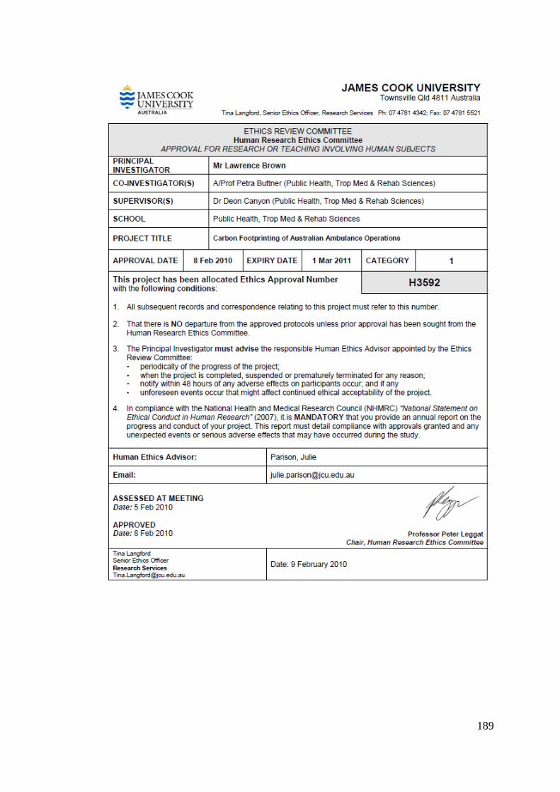
189

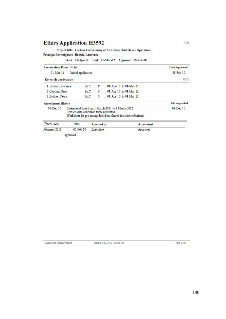
190

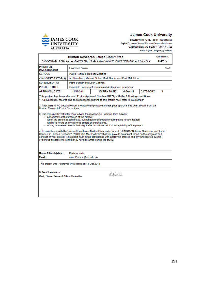
191

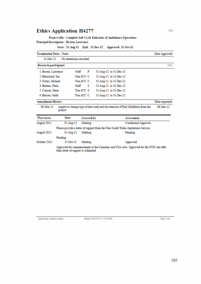
192

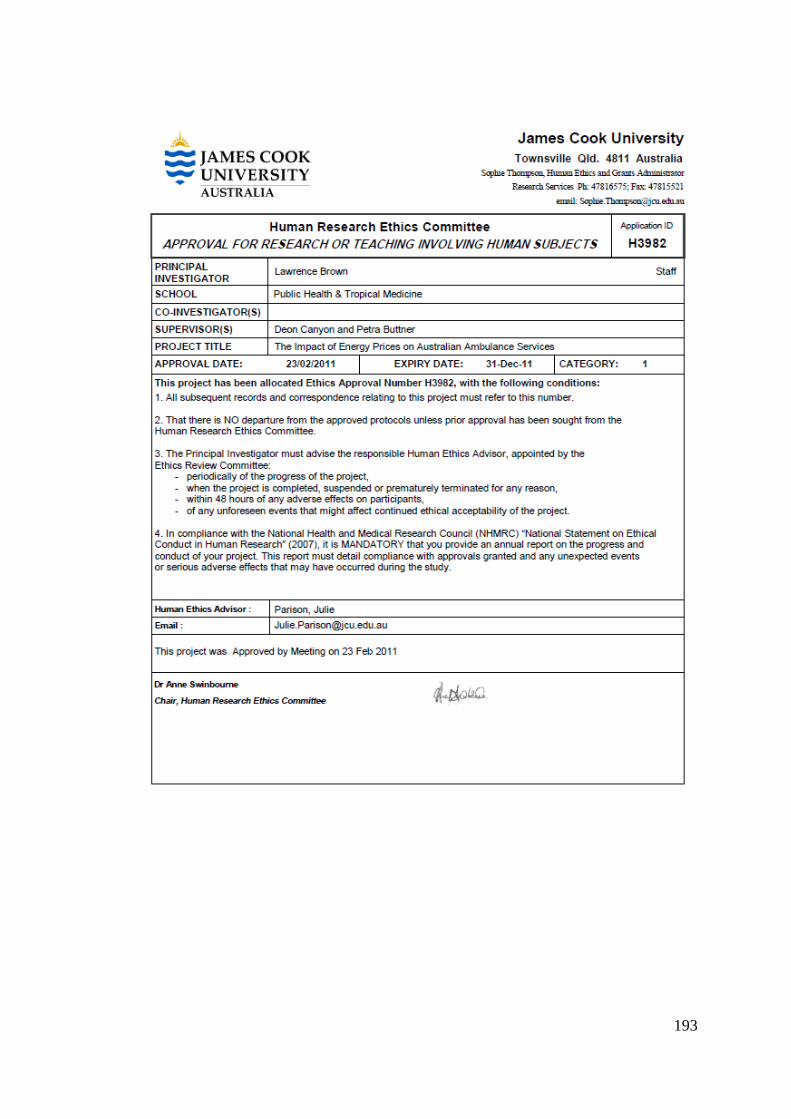
193

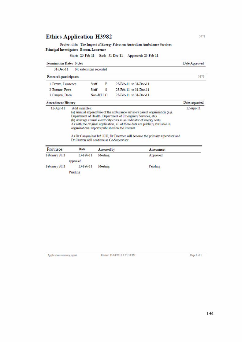
194

195

Appendix 2: Documentation of Acceptance for Manuscripts in Press Arising from

this Thesis

Brown, L.H., Canyon. D.V., Buettner, P.G. (In Press). The energy burden and

environmental impact of health services: A review. American Journal of Public Health.

Brown, L.H., Canyon. D.V., Buettner. P.G., Crawford. J.M., Judd. J., on behalf of the

Australian Ambulance Emissions Study Group. (In Press). The carbon footprint of

Australian ambulance operations. Emergency Medicine Australasia.

196

197

198

199

200

Appendix 3: Published Manuscripts Arising from or Contributing to this Thesis

Brown, L.H., Blanchard, I.E. (2012). Energy, emissions and emergency medical

services: Policy matters. Energy Policy, 46, 585-593.

201

202

203

204

205

206

207

208

209

210

Appendix 4: Contributing Author Verification of Contributions to Manuscripts

Arising from, Contributing to, or Relevant to but not Included in this Thesis

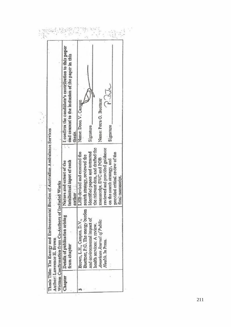
211

212

213

214

215

216

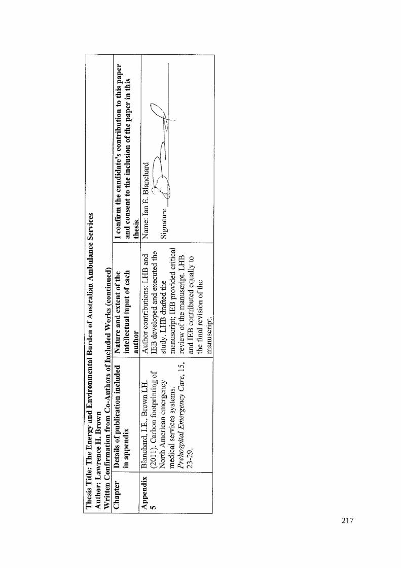
217

218

Appendix 5: Relevant Manuscripts Published by the Author but not included in

this Thesis

Blanchard, I., Brown, L.H. (2009). Carbon footprinting of EMS systems: A proof of

concept study. Prehospital Emergency Care, 13, 546-549.

Blanchard, I.E., Brown, L.H., on behalf of the North American EMS Emissions Study

Group. Carbon footprinting of North American EMS systems. (2011). Prehospital

Emergency Care, 15, 23-29.

219

220

221

222

223

224

225

226

227

228

229

230

Appendix 6: Details of Articles Included in the Literature Review (Chapter 3).

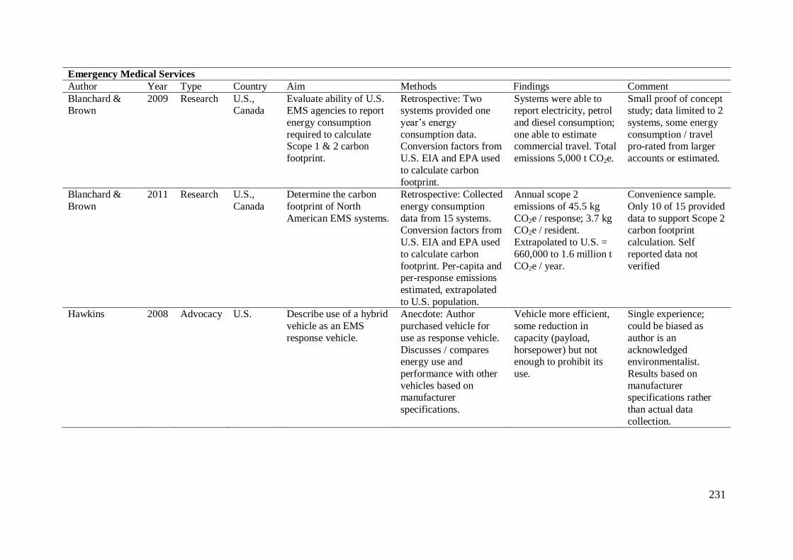
231

Emergency Medical Services

Author Year Type Country Aim Methods Findings Comment

Blanchard & Brown

2009 Research U.S., Canada

Evaluate ability of U.S. EMS agencies to report

energy consumption

required to calculate Scope 1 & 2 carbon

footprint.

Retrospective: Two systems provided one

year’s energy

consumption data. Conversion factors from

U.S. EIA and EPA used

to calculate carbon

footprint.

Systems were able to report electricity, petrol

and diesel consumption;

one able to estimate commercial travel. Total

emissions 5,000 t CO2e.

Small proof of concept study; data limited to 2

systems, some energy

consumption / travel pro-rated from larger

accounts or estimated.

Blanchard &

Brown

2011 Research U.S.,

Canada

Determine the carbon

footprint of North

American EMS systems.

Retrospective: Collected

energy consumption

data from 15 systems. Conversion factors from

U.S. EIA and EPA used

to calculate carbon

footprint. Per-capita and per-response emissions

estimated, extrapolated

to U.S. population.

Annual scope 2

emissions of 45.5 kg

CO2e / response; 3.7 kg CO2e / resident.

Extrapolated to U.S. =

660,000 to 1.6 million t

CO2e / year.

Convenience sample.

Only 10 of 15 provided

data to support Scope 2 carbon footprint

calculation. Self

reported data not

verified

Hawkins 2008 Advocacy U.S. Describe use of a hybrid

vehicle as an EMS

response vehicle.

Anecdote: Author

purchased vehicle for

use as response vehicle.

Discusses / compares energy use and

performance with other

vehicles based on manufacturer

specifications.

Vehicle more efficient,

some reduction in

capacity (payload,

horsepower) but not enough to prohibit its

use.

Single experience;

could be biased as

author is an

acknowledged environmentalist.

Results based on

manufacturer specifications rather

than actual data

collection.

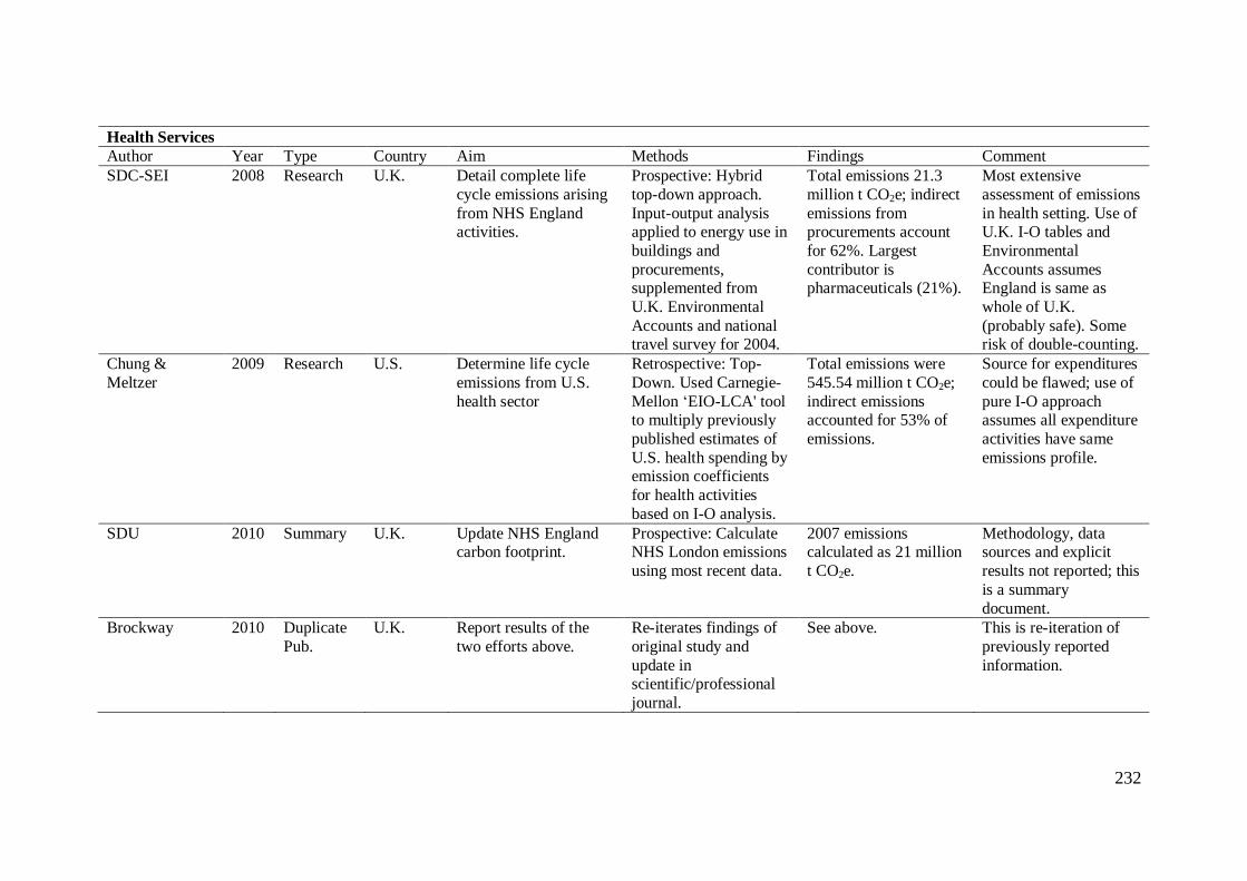
232

Health Services

Author Year Type Country Aim Methods Findings Comment

SDC-SEI 2008 Research U.K. Detail complete life

cycle emissions arising

from NHS England activities.

Prospective: Hybrid

top-down approach.

Input-output analysis applied to energy use in

buildings and

procurements, supplemented from

U.K. Environmental

Accounts and national travel survey for 2004.

Total emissions 21.3

million t CO2e; indirect

emissions from procurements account

for 62%. Largest

contributor is pharmaceuticals (21%).

Most extensive

assessment of emissions

in health setting. Use of U.K. I-O tables and

Environmental

Accounts assumes England is same as

whole of U.K.

(probably safe). Some risk of double-counting.

Chung &

Meltzer

2009 Research U.S. Determine life cycle

emissions from U.S.

health sector

Retrospective: Top-

Down. Used Carnegie-

Mellon ‘EIO-LCA' tool to multiply previously

published estimates of

U.S. health spending by emission coefficients

for health activities

based on I-O analysis.

Total emissions were

545.54 million t CO2e;

indirect emissions accounted for 53% of

emissions.

Source for expenditures

could be flawed; use of

pure I-O approach assumes all expenditure

activities have same

emissions profile.

SDU 2010 Summary U.K. Update NHS England carbon footprint.

Prospective: Calculate NHS London emissions

using most recent data.

2007 emissions calculated as 21 million

t CO2e.

Methodology, data sources and explicit

results not reported; this

is a summary

document.

Brockway 2010 Duplicate

Pub.

U.K. Report results of the

two efforts above.

Re-iterates findings of

original study and

update in scientific/professional

journal.

See above. This is re-iteration of

previously reported

information.

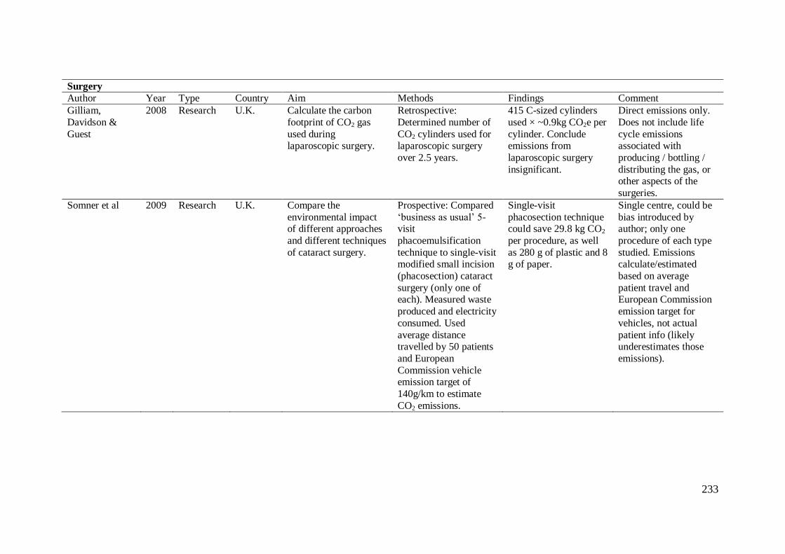
233

Surgery

Author Year Type Country Aim Methods Findings Comment

Gilliam,

Davidson &

Guest

2008 Research U.K. Calculate the carbon

footprint of CO2 gas

used during laparoscopic surgery.

Retrospective:

Determined number of

CO2 cylinders used for laparoscopic surgery

over 2.5 years.

415 C-sized cylinders

used × ~0.9kg CO2e per

cylinder. Conclude emissions from

laparoscopic surgery

insignificant.

Direct emissions only.

Does not include life

cycle emissions associated with

producing / bottling /

distributing the gas, or other aspects of the

surgeries.

Somner et al 2009 Research U.K. Compare the

environmental impact of different approaches

and different techniques

of cataract surgery.

Prospective: Compared

‘business as usual’ 5-visit

phacoemulsification

technique to single-visit modified small incision

(phacosection) cataract

surgery (only one of each). Measured waste

produced and electricity

consumed. Used

average distance travelled by 50 patients

and European

Commission vehicle emission target of

140g/km to estimate

CO2 emissions.

Single-visit

phacosection technique could save 29.8 kg CO2

per procedure, as well

as 280 g of plastic and 8 g of paper.

Single centre, could be

bias introduced by author; only one

procedure of each type

studied. Emissions calculate/estimated

based on average

patient travel and European Commission

emission target for

vehicles, not actual

patient info (likely underestimates those

emissions).

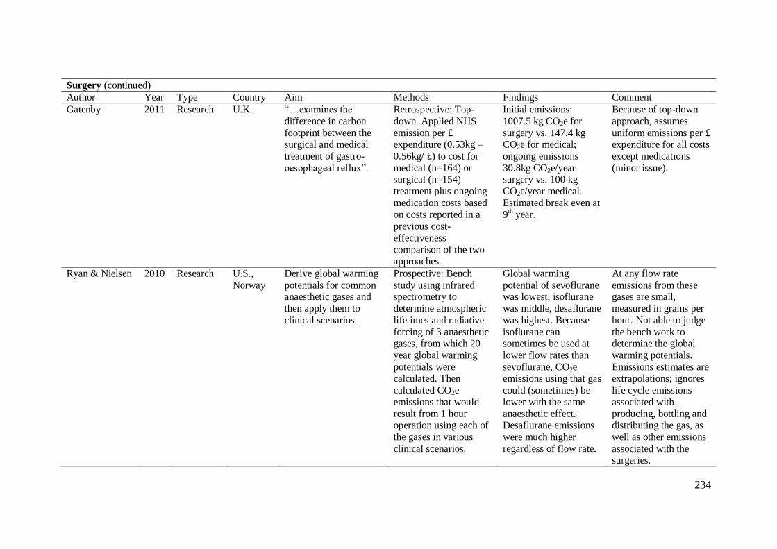
234

Surgery (continued)

Author Year Type Country Aim Methods Findings Comment

Gatenby 2011 Research U.K. “…examines the

difference in carbon

footprint between the surgical and medical

treatment of gastro-

oesophageal reflux”.

Retrospective: Top-

down. Applied NHS

emission per £ expenditure (0.53kg –

0.56kg/ £) to cost for

medical (n=164) or surgical (n=154)

treatment plus ongoing

medication costs based on costs reported in a

previous cost-

effectiveness

comparison of the two approaches.

Initial emissions:

1007.5 kg CO2e for

surgery vs. 147.4 kg CO2e for medical;

ongoing emissions

30.8kg CO2e/year surgery vs. 100 kg

CO2e/year medical.

Estimated break even at 9

th year.

Because of top-down

approach, assumes

uniform emissions per £ expenditure for all costs

except medications

(minor issue).

Ryan & Nielsen 2010 Research U.S.,

Norway

Derive global warming

potentials for common anaesthetic gases and

then apply them to

clinical scenarios.

Prospective: Bench

study using infrared spectrometry to

determine atmospheric

lifetimes and radiative

forcing of 3 anaesthetic gases, from which 20

year global warming

potentials were calculated. Then

calculated CO2e

emissions that would

result from 1 hour operation using each of

the gases in various

clinical scenarios.

Global warming

potential of sevoflurane was lowest, isoflurane

was middle, desaflurane

was highest. Because

isoflurane can sometimes be used at

lower flow rates than

sevoflurane, CO2e emissions using that gas

could (sometimes) be

lower with the same

anaesthetic effect. Desaflurane emissions

were much higher

regardless of flow rate.

At any flow rate

emissions from these gases are small,

measured in grams per

hour. Not able to judge

the bench work to determine the global

warming potentials.

Emissions estimates are extrapolations; ignores

life cycle emissions

associated with

producing, bottling and distributing the gas, as

well as other emissions

associated with the surgeries.

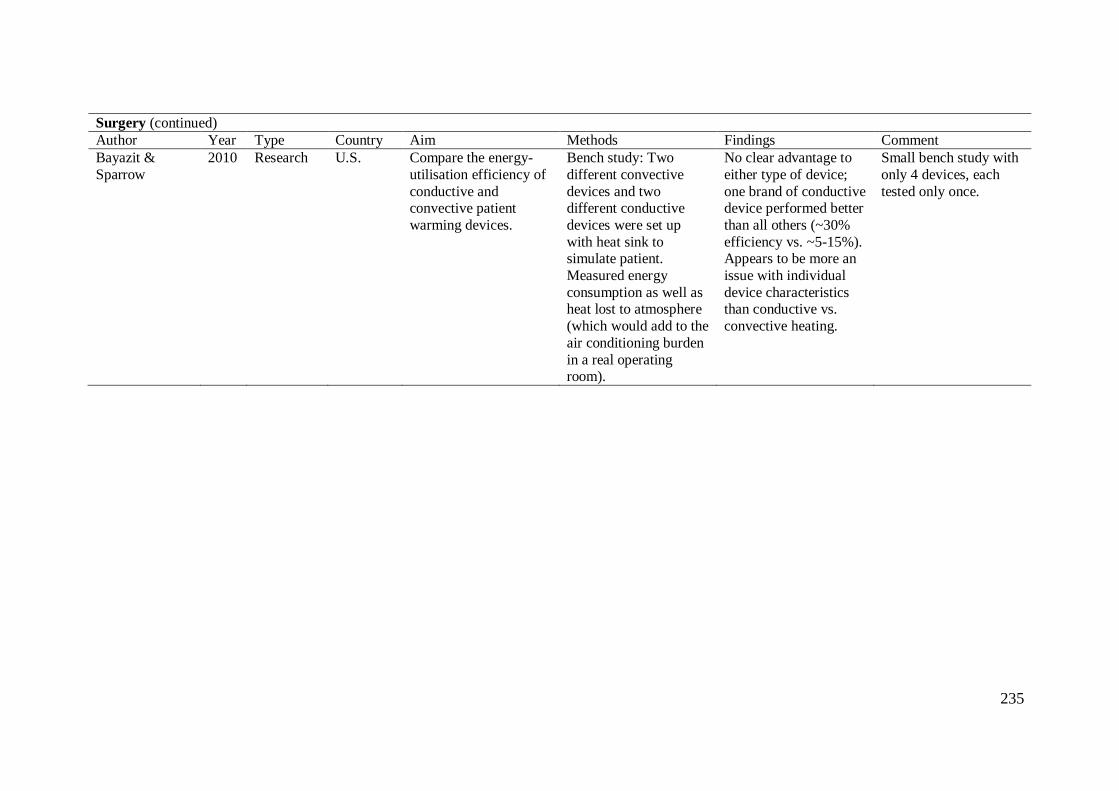
235

Surgery (continued)

Author Year Type Country Aim Methods Findings Comment

Bayazit &

Sparrow

2010 Research U.S. Compare the energy-

utilisation efficiency of

conductive and convective patient

warming devices.

Bench study: Two

different convective

devices and two different conductive

devices were set up

with heat sink to simulate patient.

Measured energy

consumption as well as heat lost to atmosphere

(which would add to the

air conditioning burden

in a real operating room).

No clear advantage to

either type of device;

one brand of conductive device performed better

than all others (~30%

efficiency vs. ~5-15%). Appears to be more an

issue with individual

device characteristics than conductive vs.

convective heating.

Small bench study with

only 4 devices, each

tested only once.

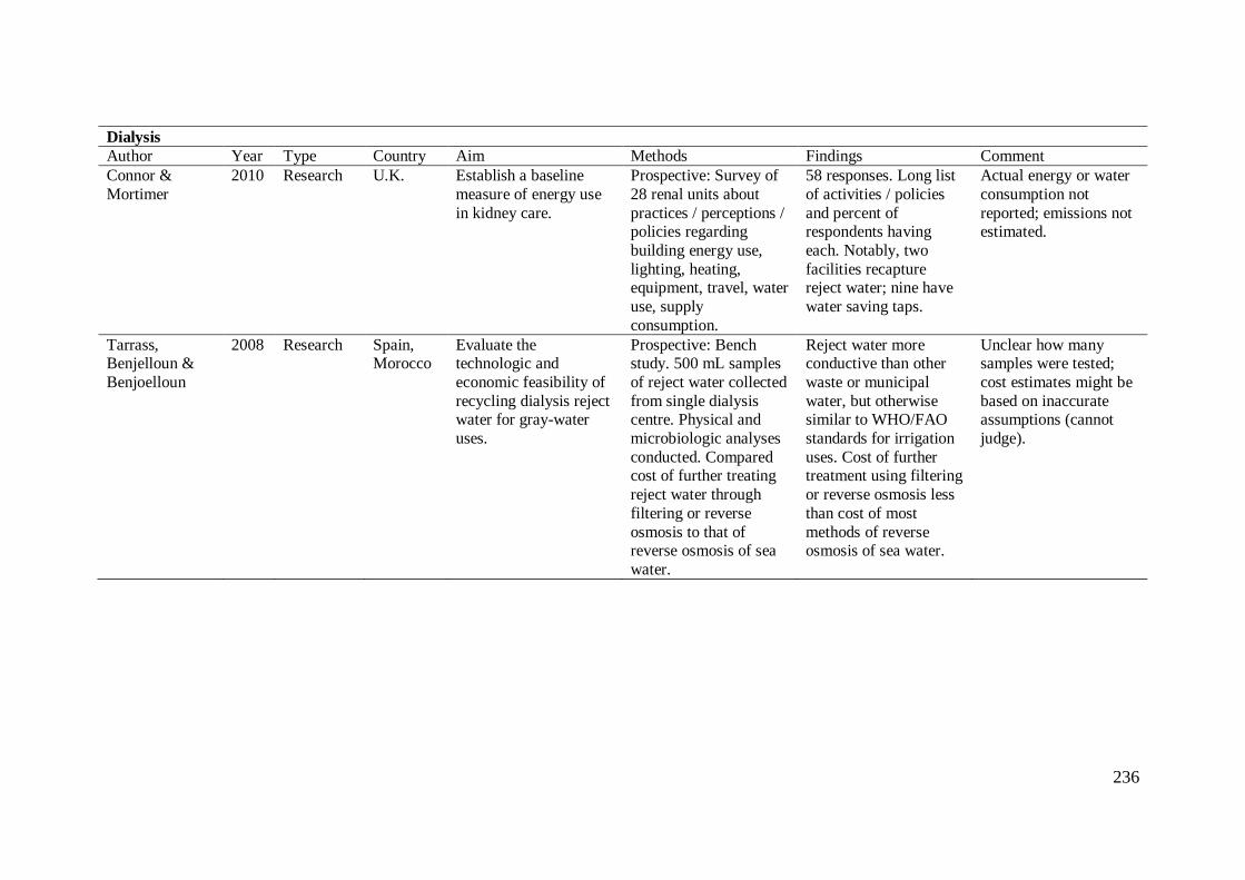
236

Dialysis

Author Year Type Country Aim Methods Findings Comment

Connor &

Mortimer

2010 Research U.K. Establish a baseline

measure of energy use

in kidney care.

Prospective: Survey of

28 renal units about

practices / perceptions / policies regarding

building energy use,

lighting, heating, equipment, travel, water

use, supply

consumption.

58 responses. Long list

of activities / policies

and percent of respondents having

each. Notably, two

facilities recapture reject water; nine have

water saving taps.

Actual energy or water

consumption not

reported; emissions not estimated.

Tarrass, Benjelloun &

Benjoelloun

2008 Research Spain, Morocco

Evaluate the technologic and

economic feasibility of

recycling dialysis reject water for gray-water

uses.

Prospective: Bench study. 500 mL samples

of reject water collected

from single dialysis centre. Physical and

microbiologic analyses

conducted. Compared cost of further treating

reject water through

filtering or reverse

osmosis to that of reverse osmosis of sea

water.

Reject water more conductive than other

waste or municipal

water, but otherwise similar to WHO/FAO

standards for irrigation

uses. Cost of further treatment using filtering

or reverse osmosis less

than cost of most

methods of reverse osmosis of sea water.

Unclear how many samples were tested;

cost estimates might be

based on inaccurate assumptions (cannot

judge).

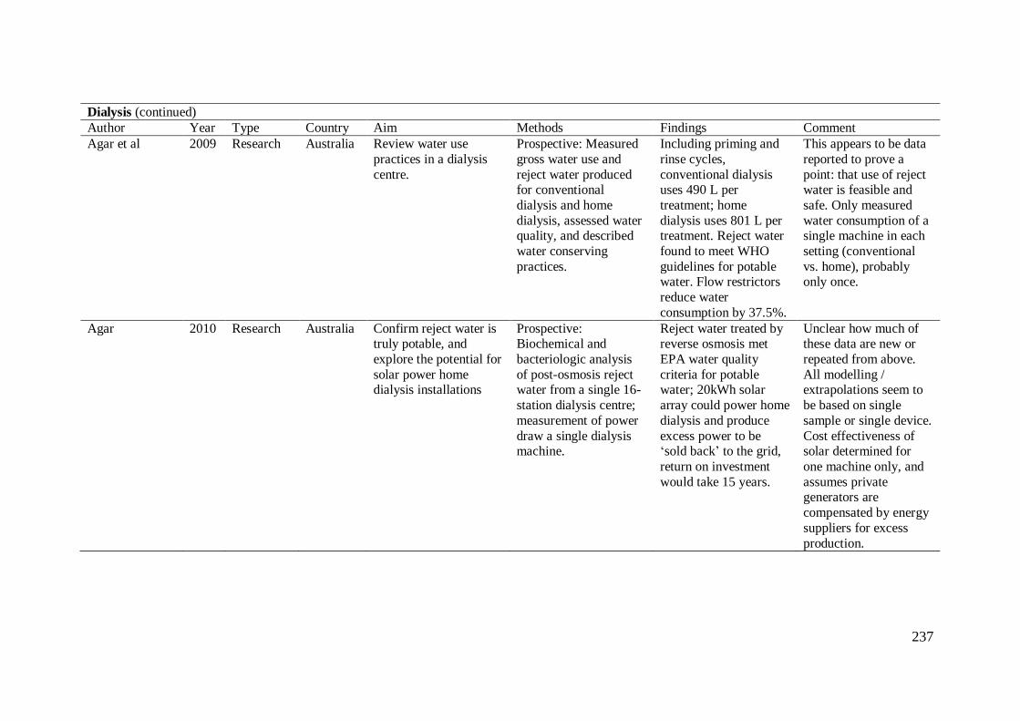
237

Dialysis (continued)

Author Year Type Country Aim Methods Findings Comment

Agar et al 2009 Research Australia Review water use

practices in a dialysis

centre.

Prospective: Measured

gross water use and

reject water produced for conventional

dialysis and home

dialysis, assessed water quality, and described

water conserving

practices.

Including priming and

rinse cycles,

conventional dialysis uses 490 L per

treatment; home

dialysis uses 801 L per treatment. Reject water

found to meet WHO

guidelines for potable water. Flow restrictors

reduce water

consumption by 37.5%.

This appears to be data

reported to prove a

point: that use of reject water is feasible and

safe. Only measured

water consumption of a single machine in each

setting (conventional

vs. home), probably only once.

Agar 2010 Research Australia Confirm reject water is truly potable, and

explore the potential for

solar power home dialysis installations

Prospective: Biochemical and

bacteriologic analysis

of post-osmosis reject water from a single 16-

station dialysis centre;

measurement of power

draw a single dialysis machine.

Reject water treated by reverse osmosis met

EPA water quality

criteria for potable water; 20kWh solar

array could power home

dialysis and produce

excess power to be ‘sold back’ to the grid,

return on investment

would take 15 years.

Unclear how much of these data are new or

repeated from above.

All modelling / extrapolations seem to

be based on single

sample or single device.

Cost effectiveness of solar determined for

one machine only, and

assumes private generators are

compensated by energy

suppliers for excess

production.

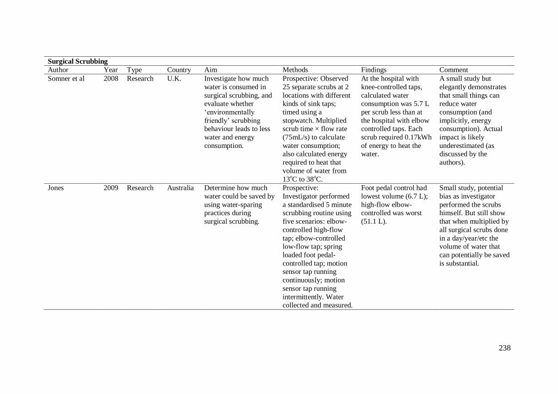
238

Surgical Scrubbing

Author Year Type Country Aim Methods Findings Comment

Somner et al 2008 Research U.K. Investigate how much

water is consumed in

surgical scrubbing, and evaluate whether

‘environmentally

friendly’ scrubbing behaviour leads to less

water and energy

consumption.

Prospective: Observed

25 separate scrubs at 2

locations with different kinds of sink taps;

timed using a

stopwatch. Multiplied scrub time × flow rate

(75mL/s) to calculate

water consumption; also calculated energy

required to heat that

volume of water from

13oC to 38

oC.

At the hospital with

knee-controlled taps,

calculated water consumption was 5.7 L

per scrub less than at

the hospital with elbow controlled taps. Each

scrub required 0.17kWh

of energy to heat the water.

A small study but

elegantly demonstrates

that small things can reduce water

consumption (and

implicitly, energy consumption). Actual

impact is likely

underestimated (as discussed by the

authors).

Jones 2009 Research Australia Determine how much

water could be saved by

using water-sparing practices during

surgical scrubbing.

Prospective:

Investigator performed

a standardised 5 minute scrubbing routine using

five scenarios: elbow-

controlled high-flow

tap; elbow-controlled low-flow tap; spring

loaded foot pedal-

controlled tap; motion sensor tap running

continuously; motion

sensor tap running

intermittently. Water collected and measured.

Foot pedal control had

lowest volume (6.7 L);

high-flow elbow-controlled was worst

(51.1 L).

Small study, potential

bias as investigator

performed the scrubs himself. But still show

that when multiplied by

all surgical scrubs done

in a day/year/etc the volume of water that

can potentially be saved

is substantial.

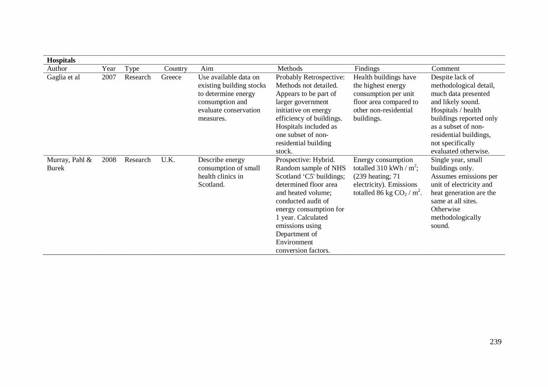
239

Hospitals

Author Year Type Country Aim Methods Findings Comment

Gaglia et al 2007 Research Greece Use available data on

existing building stocks

to determine energy consumption and

evaluate conservation

measures.

Probably Retrospective:

Methods not detailed.

Appears to be part of larger government

initiative on energy

efficiency of buildings. Hospitals included as

one subset of non-

residential building stock.

Health buildings have

the highest energy

consumption per unit floor area compared to

other non-residential

buildings.

Despite lack of

methodological detail,

much data presented and likely sound.

Hospitals / health

buildings reported only as a subset of non-

residential buildings,

not specifically evaluated otherwise.

Murray, Pahl &

Burek

2008 Research U.K. Describe energy

consumption of small

health clinics in Scotland.

Prospective: Hybrid.

Random sample of NHS

Scotland ‘C5' buildings; determined floor area

and heated volume;

conducted audit of energy consumption for

1 year. Calculated

emissions using

Department of Environment

conversion factors.

Energy consumption

totalled 310 kWh / m2;

(239 heating; 71 electricity). Emissions

totalled 86 kg CO2 / m2.

Single year, small

buildings only.

Assumes emissions per unit of electricity and

heat generation are the

same at all sites. Otherwise

methodologically

sound.

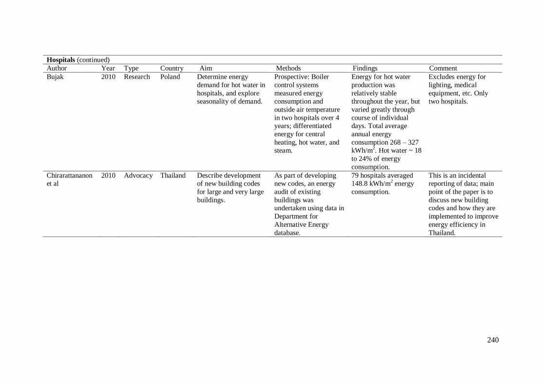
240

Hospitals (continued)

Author Year Type Country Aim Methods Findings Comment

Bujak 2010 Research Poland Determine energy

demand for hot water in

hospitals, and explore seasonality of demand.

Prospective: Boiler

control systems

measured energy consumption and

outside air temperature

in two hospitals over 4 years; differentiated

energy for central

heating, hot water, and steam.

Energy for hot water

production was

relatively stable throughout the year, but

varied greatly through

course of individual days. Total average

annual energy

consumption 268 – 327 kWh/m

2. Hot water ~ 18

to 24% of energy

consumption.

Excludes energy for

lighting, medical

equipment, etc. Only two hospitals.

Chirarattananon et al

2010 Advocacy Thailand Describe development of new building codes

for large and very large

buildings.

As part of developing new codes, an energy

audit of existing

buildings was undertaken using data in

Department for

Alternative Energy

database.

79 hospitals averaged 148.8 kWh/m

2 energy

consumption.

This is an incidental reporting of data; main

point of the paper is to

discuss new building codes and how they are

implemented to improve

energy efficiency in

Thailand.

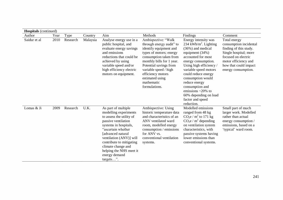
241

Hospitals (continued)

Author Year Type Country Aim Methods Findings Comment

Saidur et al 2010 Research Malaysia Analyse energy use in a

public hospital, and

evaluate energy savings and emissions

reductions that could be

achieved by using variable speed and/or

high efficiency electric

motors on equipment.

Ambispective: “Walk

through energy audit” to

identify equipment and types of motors; energy

consumption taken from

monthly bills for 1 year. Potential savings from

variable speed / high

efficiency motors estimated using

mathematic

formulations.

Energy intensity was

234 kWh/m2. Lighting

(36%) and medical equipment (34%)

accounted for most

energy consumption. Using high efficiency /

variable speed motors

could reduce energy consumption would

reduce energy

consumption and

emissions ~20% to 60% depending on load

factor and speed

reduction.

Total energy

consumption incidental

finding of this study. Single hospital; more

focused on electric

motor efficiency and how that could impact

energy consumption.

Lomas & Ji 2009 Research U.K. As part of multiple

modelling experiments

to assess the utility of

passive ventilation systems in hospitals,

“ascertain whether

[advanced natural ventilation (ANV)] will

contribute to mitigating

climate change and

helping the NHS meet it energy demand

targets…”.

Ambispective: Using

historic temperature data

and characteristics of an

ANV ventilated ward room, modelled energy

consumption / emissions

for ANV vs. conventional ventilation

systems.

Modelled emissions

ranged from 48 kg

CO2e / m2 to 171 kg

CO2e / m2 depending

on ventilation system

characteristics, with

passive systems having lower emissions than

conventional systems.

Small part of much

larger work. Modelled

rather than actual

energy consumption / emissions, based on a

‘typical’ ward room.

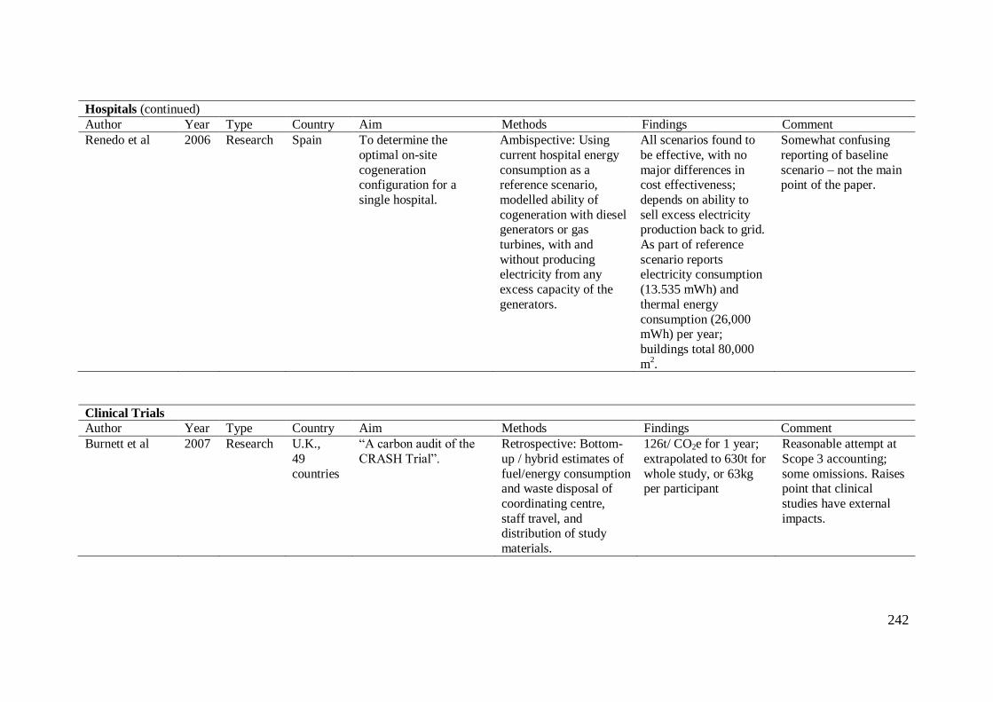
242

Hospitals (continued)

Author Year Type Country Aim Methods Findings Comment

Renedo et al 2006 Research Spain To determine the

optimal on-site

cogeneration configuration for a

single hospital.

Ambispective: Using

current hospital energy

consumption as a reference scenario,

modelled ability of

cogeneration with diesel generators or gas

turbines, with and

without producing electricity from any

excess capacity of the

generators.

All scenarios found to

be effective, with no

major differences in cost effectiveness;

depends on ability to

sell excess electricity production back to grid.

As part of reference

scenario reports electricity consumption

(13.535 mWh) and

thermal energy

consumption (26,000 mWh) per year;

buildings total 80,000

m2.

Somewhat confusing

reporting of baseline

scenario – not the main point of the paper.

Clinical Trials

Author Year Type Country Aim Methods Findings Comment

Burnett et al 2007 Research U.K.,

49

countries

“A carbon audit of the

CRASH Trial”.

Retrospective: Bottom-

up / hybrid estimates of

fuel/energy consumption and waste disposal of

coordinating centre,

staff travel, and distribution of study

materials.

126t/ CO2e for 1 year;

extrapolated to 630t for

whole study, or 63kg per participant

Reasonable attempt at

Scope 3 accounting;

some omissions. Raises point that clinical

studies have external

impacts.

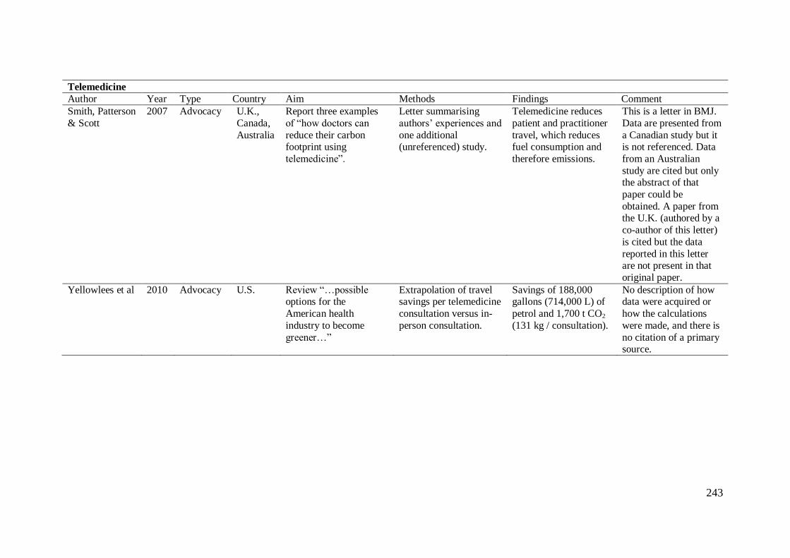
243

Telemedicine

Author Year Type Country Aim Methods Findings Comment

Smith, Patterson

& Scott

2007 Advocacy U.K.,

Canada,

Australia

Report three examples

of “how doctors can

reduce their carbon footprint using

telemedicine”.

Letter summarising

authors’ experiences and

one additional (unreferenced) study.

Telemedicine reduces

patient and practitioner

travel, which reduces fuel consumption and

therefore emissions.

This is a letter in BMJ.

Data are presented from

a Canadian study but it is not referenced. Data

from an Australian

study are cited but only the abstract of that

paper could be

obtained. A paper from the U.K. (authored by a

co-author of this letter)

is cited but the data

reported in this letter are not present in that

original paper.

Yellowlees et al 2010 Advocacy U.S. Review “…possible options for the

American health

industry to become

greener…”

Extrapolation of travel savings per telemedicine

consultation versus in-

person consultation.

Savings of 188,000 gallons (714,000 L) of

petrol and 1,700 t CO2

(131 kg / consultation).

No description of how data were acquired or

how the calculations

were made, and there is

no citation of a primary source.

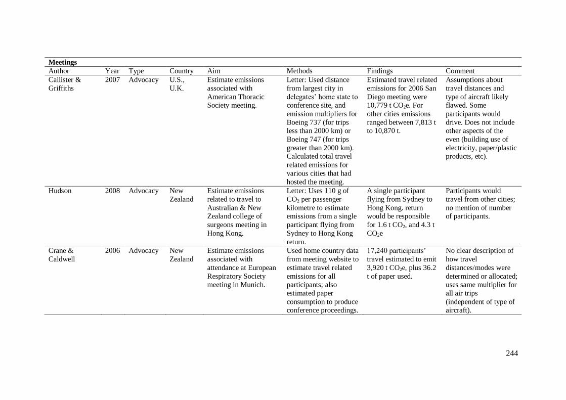
244

Meetings

Author Year Type Country Aim Methods Findings Comment

Callister &

Griffiths

2007 Advocacy U.S.,

U.K.

Estimate emissions

associated with

American Thoracic Society meeting.

Letter: Used distance

from largest city in

delegates’ home state to conference site, and

emission multipliers for

Boeing 737 (for trips less than 2000 km) or

Boeing 747 (for trips

greater than 2000 km). Calculated total travel

related emissions for

various cities that had

hosted the meeting.

Estimated travel related

emissions for 2006 San

Diego meeting were 10,779 t CO2e. For

other cities emissions

ranged between 7,813 t to 10,870 t.

Assumptions about

travel distances and

type of aircraft likely flawed. Some

participants would

drive. Does not include other aspects of the

even (building use of

electricity, paper/plastic products, etc).

Hudson 2008 Advocacy New

Zealand

Estimate emissions

related to travel to

Australian & New Zealand college of

surgeons meeting in

Hong Kong.

Letter: Uses 110 g of

CO2 per passenger

kilometre to estimate emissions from a single

participant flying from

Sydney to Hong Kong

return.

A single participant

flying from Sydney to

Hong Kong. return would be responsible

for 1.6 t CO2, and 4.3 t

CO2e

Participants would

travel from other cities;

no mention of number of participants.

Crane &

Caldwell

2006 Advocacy New

Zealand

Estimate emissions

associated with

attendance at European

Respiratory Society meeting in Munich.

Used home country data

from meeting website to

estimate travel related

emissions for all participants; also

estimated paper

consumption to produce conference proceedings.

17,240 participants’

travel estimated to emit

3,920 t CO2e, plus 36.2

t of paper used.

No clear description of

how travel

distances/modes were

determined or allocated; uses same multiplier for

all air trips

(independent of type of aircraft).

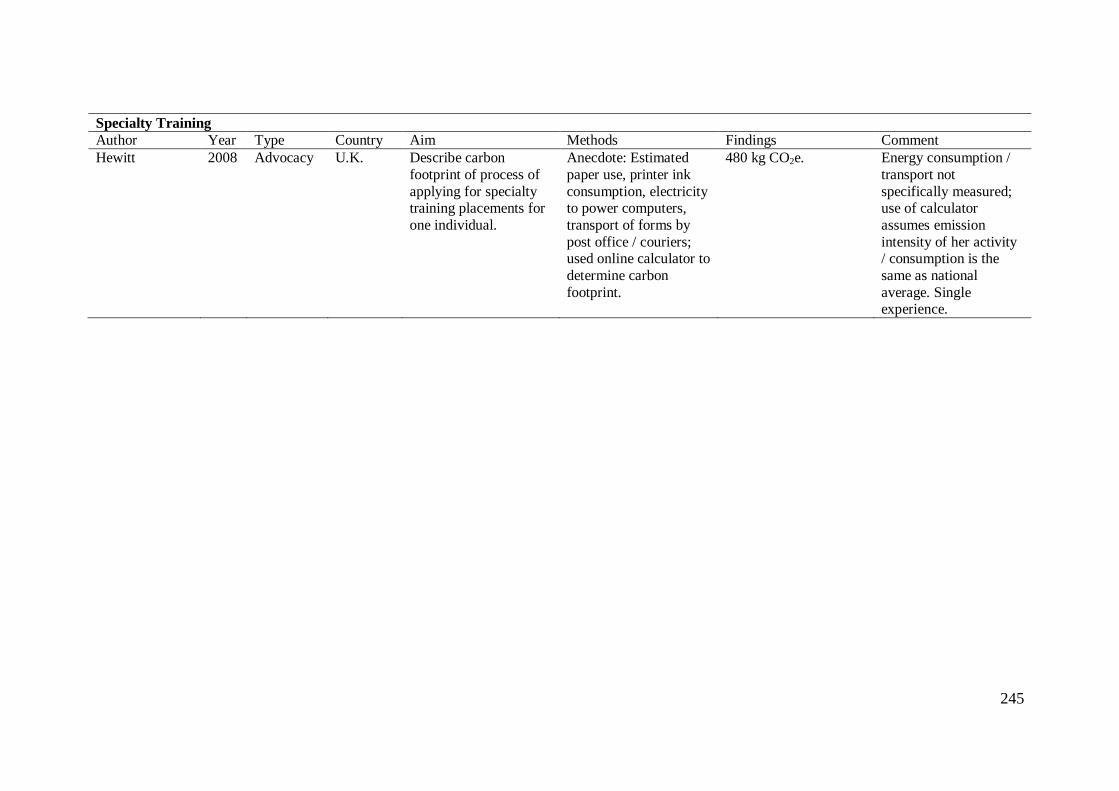
245

Specialty Training

Author Year Type Country Aim Methods Findings Comment

Hewitt 2008 Advocacy U.K. Describe carbon

footprint of process of

applying for specialty training placements for

one individual.

Anecdote: Estimated

paper use, printer ink

consumption, electricity to power computers,

transport of forms by

post office / couriers; used online calculator to

determine carbon

footprint.

480 kg CO2e. Energy consumption /

transport not

specifically measured; use of calculator

assumes emission

intensity of her activity / consumption is the

same as national

average. Single experience.

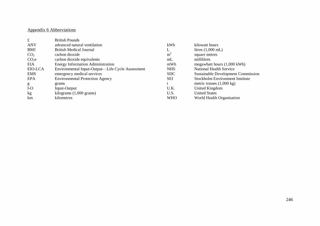
246

Appendix 6 Abbreviations

£ British Pounds

ANV advanced natural ventilation BMJ British Medical Journal

CO2 carbon dioxide

CO2e carbon dioxide equivalents

EIA Energy Information Administration EIO-LCA Environmental Input-Output—Life Cycle Assessment

EMS emergency medical services

EPA Environmental Protection Agency g grams

I-O Input-Output

kg kilograms (1,000 grams) km kilometres

kWh kilowatt hours L litres (1,000 mL)

m2 square metres

mL millilitres

mWh megawhatt hours (1,000 kWh) NHS National Health Service

SDC Sustainable Development Commission

SEI Stockholm Environment Institute t metric tonnes (1,000 kg)

U.K. United Kingdom

U.S. United States WHO World Health Organisation

247

Appendix 7: Data collection tool and pro-rating worksheet for the study of

Australian Scope 1 and Scope 2 energy consumption and greenhouse gas emissions

(Chapter 4).

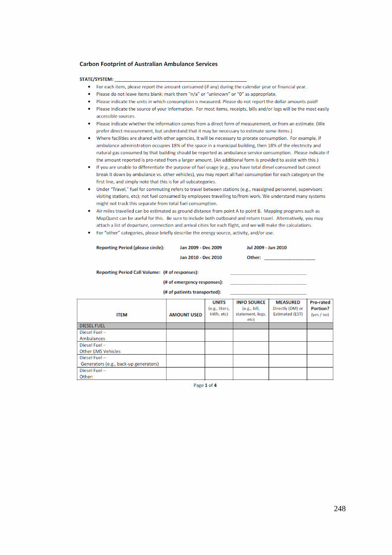
248

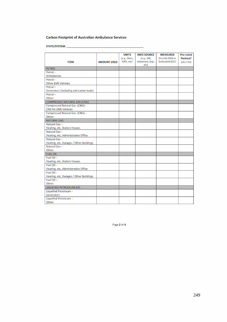
249

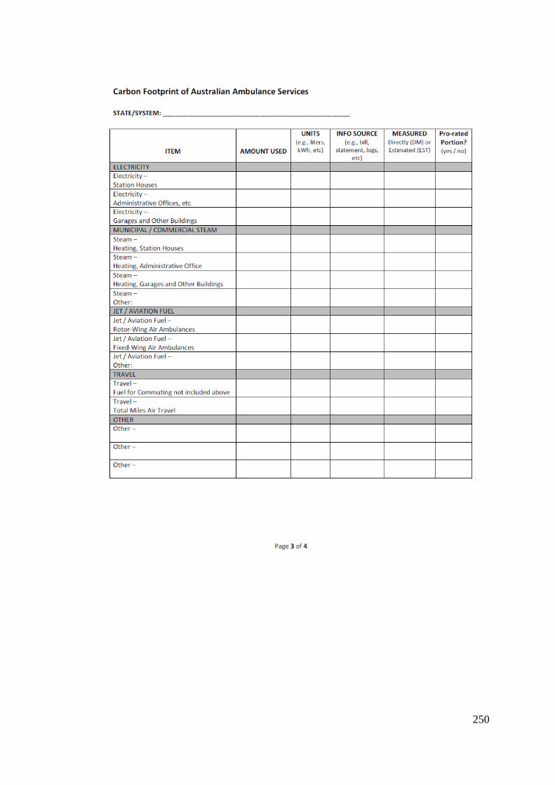
250

251

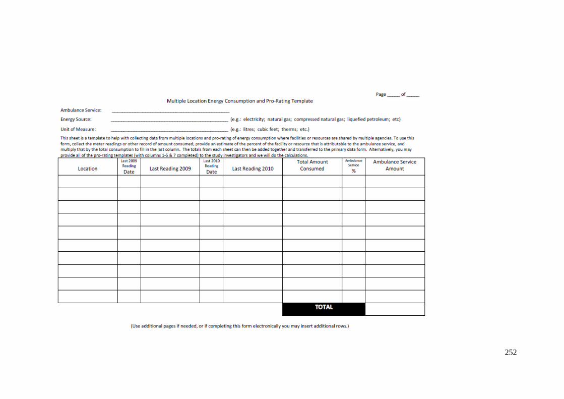
252