ADA44 87 DESIGN AND CONSTRUCTON or A TRUCK ARRESTER BED /RESEARCH FACL IYU , NNSOYL V AIA S TATE UNIV UNIVERSITY

PARK REPT OF ME HANCAL ENGINEERING M S T RUERLOOD

UITE U0 AUG R4 RUE 14 U A 0083 F/A 13/2 NmEEE @oss3 hmE.E.IEolhshmmElmEIMEEK'molso

1.0 :1.8

MICR(XCPY RLSOLU11ON ILST CHARI

t 4r

,A'ftE.',$,.

A4 mVM

082

The Pennsylvania State University

The Graduate School

Department of Mechanical Engineering

August 10, 1984

Design and Construction

of a

Truck Arrester Bed

Research Facility

A Report in

Mechanical Engineering

by

Michael S. Trueblood

DTIC rSubmitted in Partial Fulfillment ELECT ,

of the Requirements Efor the Degree of AUG281984

Master of Engineering

D

Date i Approval ames C. WamboldProfessor of Mechanical EngineeringGraduate Advisor

Pi. ;'I did I-IS 11'

2'

ACKNOWLEDGEMENTS

The author would like to thank Dr. James C. Wambold of The Pennsylvania

State University for his support in the preparation of this report. Special

thanks go to the Pennsylvania Transportation Institute for its help and

support, to the Pennsylvania Department of Transportation for its involvement

in the project, to the sponsor of the project, the Federal Highway

Administration, and to the builders of the track, Herbert R. Imbt, Inc. In

addition, I would like to thank Sara Casey for her efforts in typing this

report.

Finally, I am grateful for the support and encouragement given by my

wife, Karen, and our children, Jonathan, Matthew, Heather, and Brian. This

report is dedicated to them.

Accession For -

NTIS CGA&I

DTIC TAB

UI I10 Lit i2 d r

Distribution/ 2

Availability Codes 04Avail and/or

Dist Special

ABSTRACT

Ouring the summer of 1984, an Arrester Bed Research Facility was

constructed adjacent to the Pavement Durability Research Facility of the

Pennsylvania Transportation Institute. The Arrester Bed Research Facility is

to be ised for experimentation in the mechanism of stopping runaway vehicles

with escape ramps. The results of the study will be empirically-substantiated

criteria for the design of highway escape ramps. This report is the first

segment of a paper which will include descriptions of 1) construction of the

arrester bed, 2) experiments performed, 3) analysis and presentation of

results, and 4) recommended design criteria. Specific items covered in this

first report are ') background information, 2) design description, 3)

construction phase elements, and 4) work sampling studies and productivity

reports.

* r-i *

iii

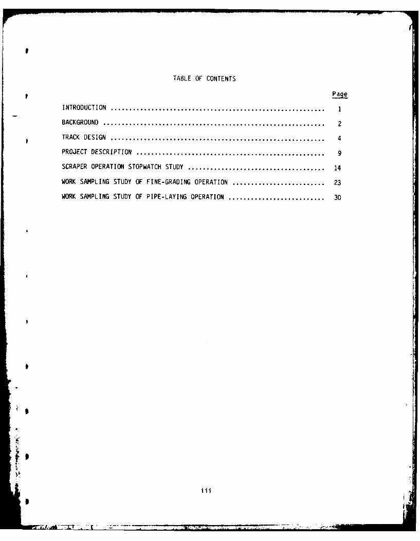
TABLE OF CONTENTS

Page

INTRODUCTION .... ...................................................... 1

BACKGROUND .. ........................................................ 2

TRACK DESIGN...................................................... 4

PROJECT DESCRIPTION................................................. 9

SCRAPER OPERATION STOPWATCH STUDY ..................................... 14

WORK SAMPLING STUDY OF FINE-GRADING OPERATION ......................... 23

WORK SAMPLING STUDY OF PIPE-LAYING OPERATION .......................... 30

iii

INTRODUCTION

This report describes the construction phase of the Arrester Bed Research

Facility of the Pennsylvania Transportation Institute. As a preliminary, some

background information is provided which discusses the need for such a

facility. Next, the track design is explained. A project description is

included with a daily account of construction progress. During the course of

the project, three major operations (excavation, fine-grading, and pipe-

laying) were analyzed in detail. The results of the studies are included as

separate chapters.

~9,4~I

BACKUROUND

On highways with long, steep down-grades, heavy vehicles such as trucks

and tractor-trailers occasionally lose their braking capabilities, and become

so-called runaway trucks. These vehicles, if not properly stopped, can cause

loss of life and extensive property damage.

Efforts have been made in the last twenty years to solve the problems

associated with stopping runaway vehicles. Usually, truck escape ramps with

beds of gravel, sand, or dirt have been built near the road. Trucks may be

driven into the beds and stopped by the grade and drag forces of the beds.

Although some other methods have been suggested (such as chain arrester

systems and hydraulic arrester systems), the escape ramp is the most effective

means of stopping runaway trucks. It is believed that the gravel-filled

arrester bed (followed by the sand pile and then the gravity ramnp) is the most

effective type of escape ramp. Of the three types of ramps, the gravity ramp

is usually the most expensive, then the gravel arrester bed, with the sand

pile being the least expensive. The gravel arrester bed, considering its cost

and performance, is the most cost-effective ramp. The maintenance of truck

escape ramps costs very little compared to other options for stopping runaway

vehicles.

However, the fundamental understanding of the mechanisms involved in

stopping runaway vehicles is limited, and does not yet yield precise

specifications for design. Field testing has been done primarily to evaluate

the performance of a specific ramp rather than to extend basic knowledge. A

microscopic study of the stopping mechanisms has never been performed to

analyze the relationship between drag force and its related factors.

It has been recommended that research be undertaken to improve the

understanding of the mechanism of stopping runaway vehicles by escape ramps,

so that adequate design can be achieved, and overdesign avoided. In

particular, the relationship between the drag force and its related factors

(vehicle speed, contact pressure, tire size, gravel size, etc.) must be

determined so that a formula can be provided for design engineers to use in

computing the required length for an escape ramp.

2

Long-term performance of the escape ramp has not been studied. Such

monitoring might answer questions such as the percentage of fine material that

would require replacement, the service life of the gravels used in the

arrester beds, and the relationship of service life to frequency of use.

( 3

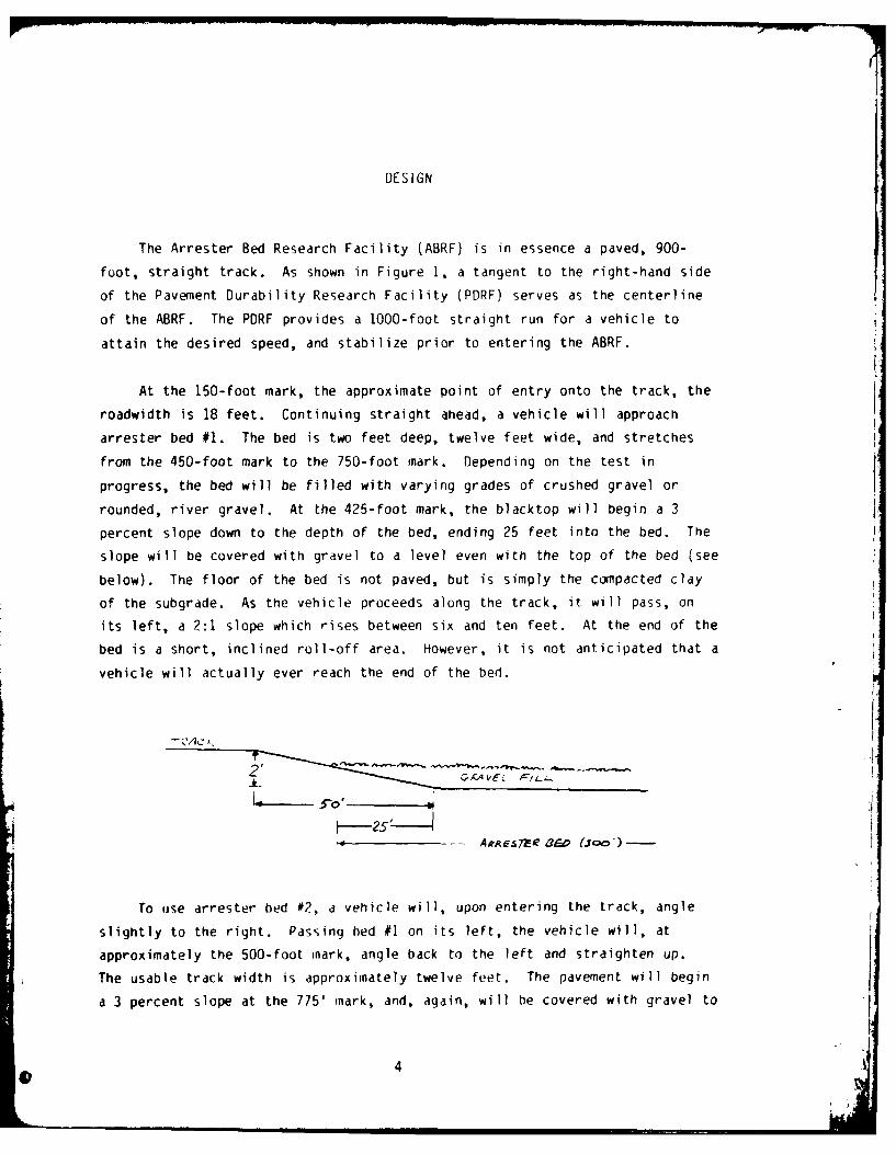
DESIGN

The Arrester Bed Research Facility (ABRF) is in essence a paved, 900-

foot, straight track. As shown in Figure 1, a tangent to the right-hand side

of the Pavement Durability Research Facility (PDRF) serves as the centerline

of the ABRF. The PDRF provides a 1000-foot straight run for a vehicle to

attain the desired speed, and stabilize prior to entering the ABRF.

At the 150-foot mark, the approximate point of entry onto the track, the

roadwidth is 18 feet. Continuing straight ahead, a vehicle will approach

arrester bed #1. The bed is two feet deep, twelve feet wide, and stretches

from the 450-foot mark to the 750-foot mark. Depending on the test inprogress, the bed will be filled with varying grades of crushed gravel orrounded, river gravel. At the 425-foot mark, the blacktop will begin a 3

percent slope down to the depth of the bed, ending 25 feet into the bed. The

slope will be covered with gravel to a level even with the top of the bed (see

below). The floor of the bed is not paved, but is simply the compacted clay

of the subgrade. As the vehicle proceeds along the track, it will pass, on

its left, a 2:1 slope which rises between six and ten feet. At the end of the

bed is a short, inclined roll-off area. However, it is not anticipated that a

vehicle will actually ever reach the end of the bed.

, .....AeAERE O (To

To use arrester bed #2, a vehicle will, upon entering the track, angle

slightly to the right. Passing hed #1 on its left, the vehicle will, at

approximately the 500-foot mark, angle back to the left and straighten up.

The usable track width is approximately twelve feet. The pavement will begin

a 3 percent slope at the 775' mark, and, again, will be covered with gravel to

0 4

I.IV1

8vU 8

( Figure 1.

5

the same level as that in the bed. At the 800-foot mark, the vehicle will be

directly over the front of the bed. Like bed #1, bed #2 is twelve feet wide,

two feet deep, and three hundred feet long. It also ends with a slightly

inclined roll-off area. The cut on the right side of the track, though in

higher ground than that on the left, was also left with a 2:1 slope.

The area in which the track is situated was formerly used as a corn

field, and the ground had a slight downward slope from right to left. Since

the track, level in the longitudinal direction, was cut out of high ground (to

bring it to the same elevation as the straightaway of the PDRF), drainage of

rainwater required special consideration. On the left side of the track, from

the 200-foot mark to the 800-foot mark, is a 1 1/2-foot ', 15 inch wide,

drainage ditch. The ditch is lined with a synthetic fE contains a 4-inch,

perforated, plastic drain pipe, and is backfilled with crushed gravel. The

track and bed #1 are tilted slightly to direct runoff . he drain. The

drain empties into a natural, low area around the 950-fu-, mark and dissipates

down the slope to the left.

The low area, a natural drainage path from right to left, centered at

about the 950-foot mark, had to be filled in (to keep the track horizontal).

In order to allow the natural drainage to continue, a 21-inch concrete cross-

pipe was installed under bed #2. Ten four-foot sections of pipe (with

unsealed joints) were placed in a 2 1/2-foot wide by 3-foot deep trench, and

the trench was then backfilled with 2B gravel. The bed is sloped slightly

from both ends so that water will be channelled to the cross-pipe trench.

Water falling outside the bed, to the left, will run down the slope and follow

the same path as that discharged by the cross-pipe. Water falling on the

right side will enter a swale which starts at the 750-foot mark, and be

channelled to the high side of the cross-pipe. Except for a low, continuous

mound to contain the gravel, the ground on either side of bed #2 slopes down

and away; on the left side, the ground slopes down to the existing slope of

the field, and, on the right side, the ground slopes into the swale which was

cut for drainage.

Figure 2 shows the typical cross-section of the road, the pavement, and

arrester bed #1.

6

Original GroundOrgnlGround Level Level

.06 normal cross slope .02 .06

TYPICAL ROAD CROSS-SECol.

d'--L- IO-2A Wearing Course

6 ~ -SCEC Bose

6 --- 2A Subbase

~-Subgrace

PAVEMENT CROSS- SECTION

Orinin I Ground Level

Original GroundLe l

riginl Grund 18"Original Ground Level

Low ide 15' Filter Fabric

Fill with 28 materialDaylight thru Embankment

TYPICAL ARRESTER BED CROSS SECTION WITH DRAINAGE SYSTEM

Figure 2.

Finally, there must be a means of extracting the vehicles from the

arrester beds. Approximately 100 feet before the start of each bed, there

will be a concrete deadman. It is intended that test personnel will be able

to anchor some sort of mobile winch to the deadman (otherwise covered by a

steel plate) which will pull the vehicles backward until they can back up

under their own power.

8dCI

PROJECT DESCRIPTION

The purpose of this project was to provide the Pennsylvania

Transportation Institute with a means of investigating the mechanism of

stopping runaway trucks on escape ramps. The construction involved several

work elements which were performed essentially during July and August of 1984.

The result is the Arrester Bed Research Facility. This section is a report

and daily account of the observed progress of the operation.

The writer made his first observation of the worksite on Wednesday, 20

June. The site was a rolling cornfield. At the edge of the Pavement

Durability Research Facility, the ground rose six to ten feet. Approximately

800 feet away, in the planned path of the track, the ground dipped into the

low area. This low area was the natural drainage path from higher fields on

the right to the lower fields on the left. Along the right side, 20-30 feet

away, is a line of full-grown trees. On the following day, 21 June, a

Caterpillar D8H dozer was moved to the site, and, during the following week, a

survey crew placed elevation markers and centerline markers along the planned

path of the track. However, the first full day of construction work was 29

June.

6/29 Friday - Today, the D8H was used to strip the topsoil from the

track. The topsoil was pushed into a row along the right side of

the track. Also, a spoil area has been cleared at about the 700'

mark on the left side of the track.

6/30 - 7/1 Weekend - Heavy rain saturated the exposed clay.

7/2 Monday - The ground was too wet to work. No on-site activity

today.

7/3 Tuesday - D8 began operation at 7:30 am, pushing still-wet clay

along the path to the low area. At 10:35, the D8 was stopped for

track cleaning, and oil leak repairs. By 2:15, the repair

operation was still in progress.

9

7/4 Wednesday - Holiday (no work).

7/5 Thursday - A Caterpillar 631B scraper was brought to the site.

The only work in progress was the D8 pushing clay along the

track. A surveyor was at the site to check the slopes of the

developing side banks. The clay was too moist at this time to

use the scraper.

7/6 Friday - no work today.

7/7 - 7/8 Weekend.

7/9 Monday - The scraper and dozer were operating in tandem to

excavate clay from the track. The clay was being dumped in the

spoil area and was being compacted by a sheep's-foot roller.

7/10 Tuesday - The scraper, dozer, and roller were operating as they

were yesterday. The track elevation was dropping steadily. The

banks were being checked periodically by the surveyor (who is

otherwise operating the roller), and are being maintained at a

2:1 slope.

7/11 Wtdnesday - The dozer, scraper, and roller were in operation

again. The track was close to subgrade level, and the low area

at the 950-foot mark was filling in.

7/12 Thursday - The dozer was the only equipment in operation today.

It was being used to smooth out the piled clay in the waste area

and fill in the low area.

7/13 Friday - Same as yesterday. The compactor has rolled the entire

track; the dozer has spread the excess clay across the waste

area, and covered it with topsoil.

7/14 - 7/15 Weekend.

C 10

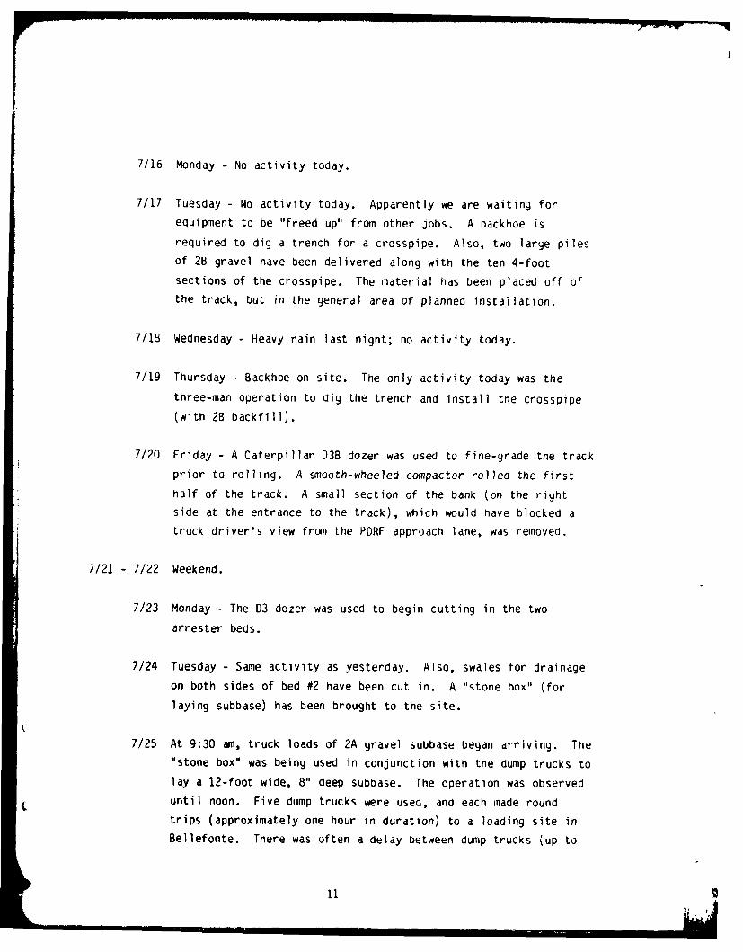
7/16 Monday - No activity today.

7/17 Tuesday - No activity today. Apparently we are waiting for

equipment to be "freed up" from other jobs. A oackhoe is

required to dig a trench for a crosspipe. Also, two large pilesof 2B gravel have been delivered along with the ten 4-foot

sections of the crosspipe. The material has been placed off ofthe track, but in the general area of planned installation.

7/18 Wednesday - Heavy rain last night; no activity today.

7/19 Thursday - Backhoe on site. The only activity today was the

three-man operation to dig the trench and install the crosspipe

(with 2B backfill).

7/20 Friday - A Caterpillar D38 dozer was used to fine-grade the track

prior to rolling. A smooth-wheeled compactor rolled the first

half of the track. A small section of the bank (on the right

side at the entrance to the track), which would have blocked a

truck driver's view fron the PDRF approach lane, was removed.

7/21 - 7/22 Weekend.

7/23 Monday - The D3 dozer was used to begin cutting in the two

arrester beds.

7/24 Tuesday - Same activity as yesterday. Also, swales for drainage

on both sides of bed #2 have been cut in. A "stone box" (for

laying subbase) has been brought to the site.

7/25 At 9:30 am, truck loads of 2A gravel subbase began arriving. The"stone box" was being used in conjunction with the dump trucks to

lay a 12-foot wide, 8" deep subbase. The operation was observed

( until noon. Five dump trucks were used, and each made round

trips (approximately one hour in duration) to a loading site in

Bellefonte. There was often a delay between dump trucks (up to

i11

20 minutes). The average operating time of the stone box (each

time a load of gravel was delivered) was 31 seconds. Over the

ten observed cycles, which spanned 1 hour-46 minutes, the "stone

box" and operator were being used productively less than 5% of

the time. Behind the "stone box", a smooth roller was compacting

the subbase. It probably would have been more efficient for the"stone box" operator to operate the roller during his 95% "free

time."

7/26 Thursday - Trench operation. Two men, one operating the backhoe,

were digging the trench for the drainpipe along the left side of

the track. The felt wrap, 4-in. plastic pipe, and 2B gravel

backfill were all on the site.

7/27 Friday - Rain. No activity.

7/28 - 7/29 Weekend.

7/30 Monday - The trenching operation was still in progress. There

was no other activity at the site.

7/31 Tuesday - The trenching operation was completed. The felt liner

and plastic drain pipe were installed, and backfilled with the

2B.

8/1 Wednesday - A Caterpillar 14E road grader was brought to the site

to taper the subbase into the beds. The taper is a 3% slope

starting 25 feet before the beds, and ending 25 feet into them.

The rest of the subbase was moistened with a watering truck, fine

graded with the grader, and rolled. Today was the last day of

the writer's on-site observations.

8/ The paving operation commenced.

8/ The deadmen were installed.

12

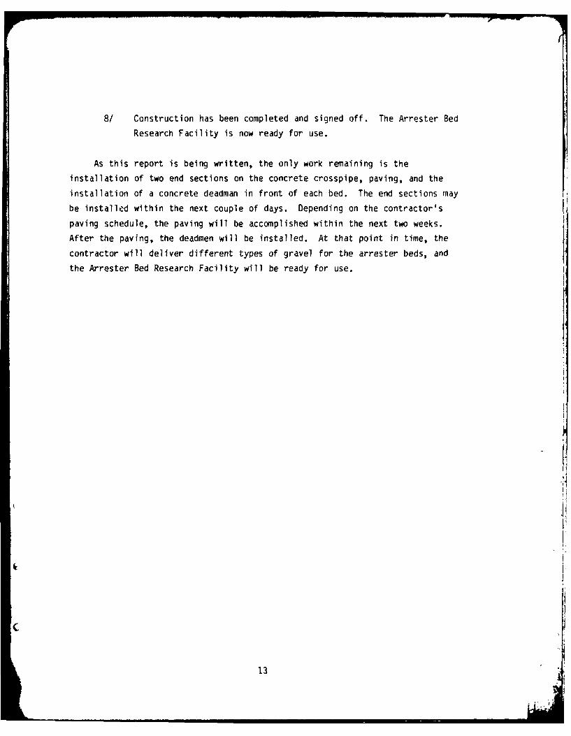
8/ Construction has been completed and signed off. The Arrester Bed

Research Facility is now ready for use.

As this report is being written, the only work remaining is the

installation of two end sections on the concrete crosspipe, paving, and the

installation of a concrete deadman in front of each bed. The end sections may

be installed within the next couple of days. Depending on the contractor's

paving schedule, the paving will be accomplished within the next two weeks.

After the paving, the deadmen will be installed. At that point in time, the

contractor will deliver different types of gravel for the arrester beds, and

the Arrester Bed Research Facility will be ready for use.

1

i I '3

SCRAPER OPERATION STOPWATCH STUDY

iI

I| II

SCRAPER OPERATION STOPWATCH STUDY

A stopwatch study was conducted during the excavation segment of the

project. The excavation was accomplished primarily with the use of a

Caterpillar 631B scraper on 9 and 10 July, and required the removal of

approximately 5000 cubic yards of sandy clay. The purpose of the study was to

determine average cycle time, average cycle element times, and delay time.

The cycle consisted of four elements: 1) the scrape (picking up dirt), 2) tne

run to the waste area, 3) the dumping of material, and 4) the return trip.

The scrape started when, with the assistance of a pusher, the scraper began to

cut into the dirt. The run started when the scraper lifted its blade, and

began moving under its own power. The dump started when the gate on the front

of the barrel was lifted. Finally, the return trip started when the gate was

dropped, and ended when the new scrape began. The duration of the observation

period was approximately six hours. During this period, 63 cycles were

recorded. Table I presents a compilation of all recorded cycle element times.

The four missing cycle element times resulted frcon incorrectly recorded

stopwatch times, and were excluded from subsequent calculations and analysis.

The table also shows the resultant means and standard deviations of the full

cycles and cycle elements. Finally, the table shows the amount of delay/break

time during the observation period.

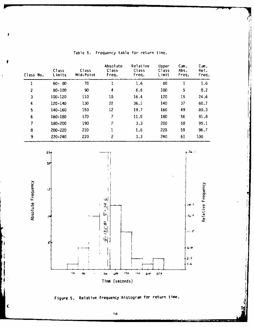
It was desired that the data be presented in graphical form (histograms).

In order to accomplish this task, the distributed data for each cycle element

and for the full cycle were divided into discrete classes (see Tables 2

through 6). The classes were chosen to be small enough in range to present a

reasonable picture of the data distribution. (See Figures 3 through 7.)

Except for the Dump Time Histogram, which is somewhat skewed to the right, the

histograms generally show the typical shape of the standard distribution.

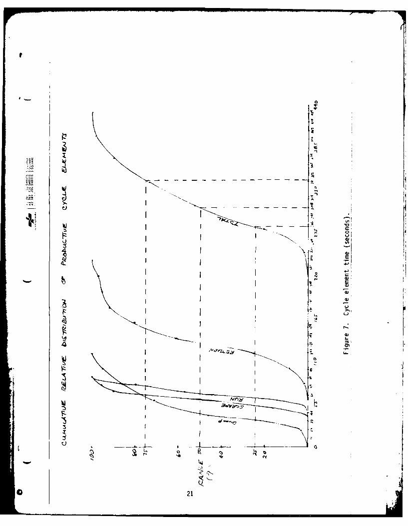
Figure 8 shows the cumulative relative distribution of the full cycles

and the cycle elements. Those curves with the more vertical slopes (scrape

and run) represent elements with more consistent durations. The lesser slopes

of the other two cycle elements may be simply explained. The observer was

positioned directly beside the scrape area. The start and stop of the

14

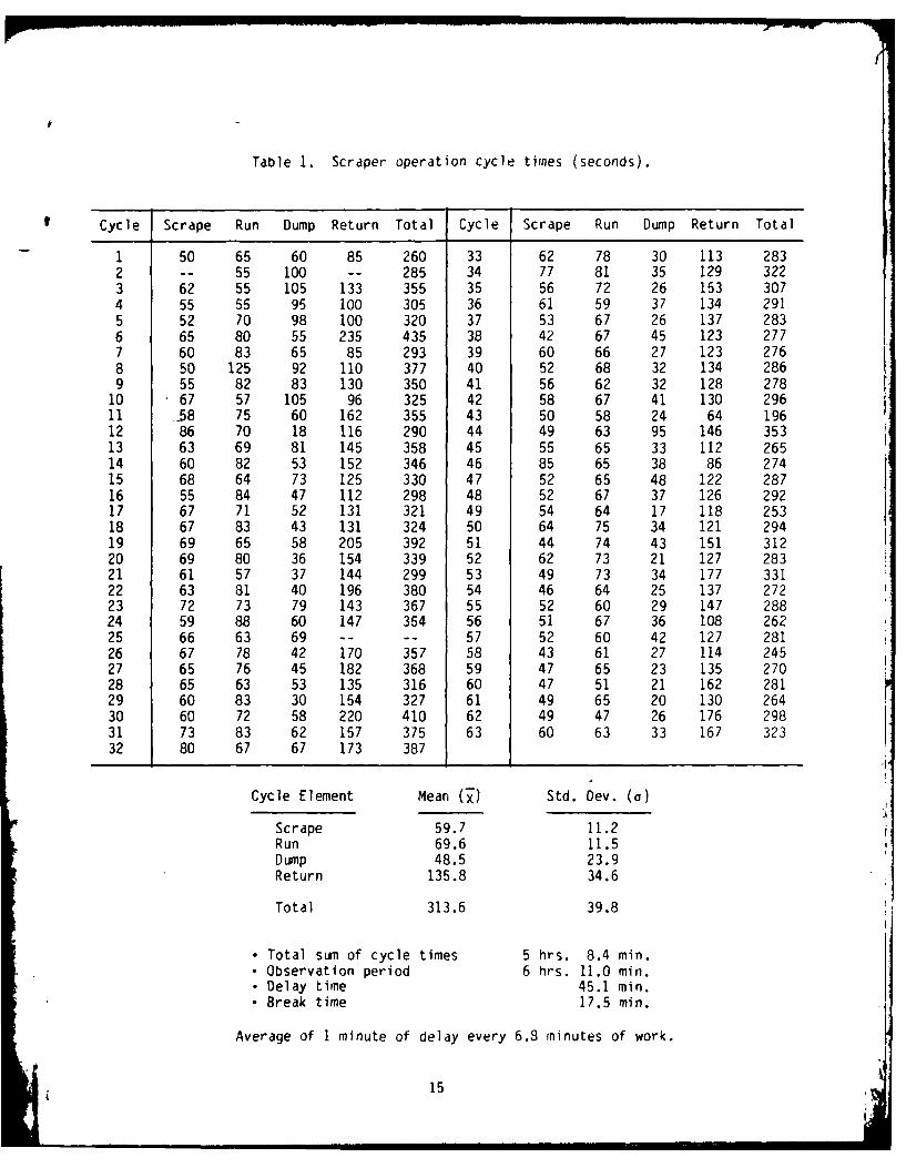
Table 1. Scraper operation cycle times (seconds).

Cycle Scrape Run Dump Return Total Cycle Scrape Run Dump Return Total

1 50 65 60 85 260 33 62 78 30 113 2832 -- 55 100 -- 285 34 77 81 35 129 3223 62 55 105 133 355 35 56 72 26 153 3074 55 55 95 100 305 36 61 59 37 134 2915 52 70 98 100 320 37 53 67 26 137 2836 65 80 55 235 435 38 42 67 45 123 2777 60 83 65 85 293 39 60 66 27 123 2768 50 125 92 110 377 40 52 68 32 134 2869 55 82 83 130 350 41 56 62 32 128 278

10 67 57 105 96 325 42 58 67 41 130 29611 58 75 60 162 355 43 50 58 24 64 19612 86 70 18 116 290 44 49 63 95 146 35313 63 69 81 145 358 45 55 65 33 112 26514 60 82 53 152 346 46 85 65 38 86 27415 68 64 73 125 330 47 52 65 48 122 28716 55 84 47 112 298 48 52 67 37 126 29217 67 71 52 131 321 49 54 64 17 118 25318 67 83 43 131 324 50 64 75 34 121 29419 69 65 58 205 392 51 44 74 43 151 31220 69 80 36 154 339 52 62 73 21 127 28321 61 57 37 144 299 53 49 73 34 177 33122 63 81 40 196 380 54 46 64 25 137 27223 72 73 79 143 367 55 52 60 29 147 28824 59 88 60 147 354 56 51 67 36 108 26225 66 63 69 -- -- 57 52 60 42 127 28126 67 78 42 170 357 58 43 61 27 114 24527 65 76 45 182 368 59 47 65 23 135 27028 65 63 53 135 316 60 47 51 21 162 28129 60 83 30 154 327 61 49 65 20 130 26430 60 72 58 220 410 62 49 47 26 176 29831 73 83 62 157 375 63 60 63 33 167 32332 80 67 67 173 387

Cycle Element Mean (7) Std. Dev. (a)

Scrape 59.7 11.2Run 69.6 11.5Dump 48.5 23.9Return 135.8 34.6

Total 313.6 39.8

- Total sum of cycle times 5 hrs. 8.4 min.- Observation period 6 hrs. 11.0 min.- Delay time 45.1 min.- Break time 17.5 min.

Average of I minute of delay every 6.8 minutes of work.

15

Table 2. Frequency table for scrape time.

Absolute Relative Upper Cum. Cum.Class Class Class Class Class Abs. Rel.

Class No. Limits Mid-Point Freq. Freq. Limit Freq. Freq.

1 40-50 45 10 16.1 50 10 16.12 50-60 55 21 33.9 60 31 50.03 60-70 65 25 40.3 70 56 90.34 70-80 75 3 4.8 80 59 95.15 80-90 85 3 4.8 90 62 100

41 Q

LA3a, I

Tim (scods

16

a, u..

• 16

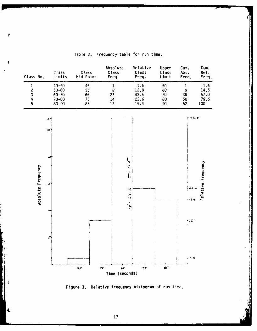
Table 3. Frequency table for run time.

Absolute Relative Upper Cum. Cum.Class Class Class Class Class Abs. Rel.

Class No. Limits Mid-Point Freq. Freq. Limit Freq. Freq.

1 40-50 45 1 1.6 50 1 1.62 50-60 55 8 12.9 60 9 14.53 60-70 65 27 43.5 70 36 57.04 70-80 75 14 22.6 80 50 79.65 80-90 85 12 19.4 90 62 100

I-.0

Ck

@17

o "*1 G)i

- i

II

F [ ./,(-

Time (seconds)

i-

Figure 3. Relative frequency histograi of run time.

17

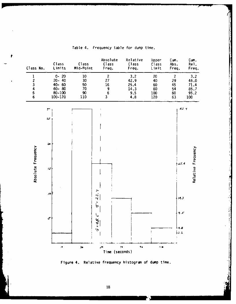
Table 4. Frequency table for dump time.

Absolute Relative Upper Cum. Cum.Class Class Class Class Class Abs. Rel.

Class No. Limits Mid-Point Freq. Freq. Limit Freq. Freq.

1 0- 20 10 2 3.2 20 2 3.22 20- 40 30 27 42.9 40 29 46.03 40- 60 50 16 25.4 60 45 71.44 60- 80 70 9 14.3 80 54 85.75 80-100 90 6 9.5 100 60 95.26 100-120 110 3 4.8 120 63 100

10 i

U (._IX >I..

I 4, "

.0

o 61

.6

Time (seconds) t

Figue 4.Relative frequency histograi of dumip time.

18

. . . . .. .. . . . ... .. ... . . . . ..... . . -L o . . . . .

Table 5. Frequency table for return time.

Absolute Relative Upper Cum. Cum.Class Class Class Class Class Abs. Rel.

Class No. Limits Mid-Point Freq. Freq. Limit Freq. Freq.

1 60- 80 70 1 1.6 80 1 1.6

2 80-100 90 4 6.6 100 5 8.2

3 100-120 110 10 16.4 120 15 24.6

4 120-140 130 22 36.1 140 37 60.7

5 140-160 150 12 19.7 160 49 80.3

6 160-180 170 7 11.5 180 56 91.8

7 180-200 190 2 3.3 200 58 95.1

8 200-220 210 1 1.6 220 59 96.7

9 220-240 220 2 3.3 240 61 100

. -

"!S"

L. I

J t : o 'M 17 -j LI z . .

i Time (seconds)

Figure 5. Relative frequency histogram for return time.

10

Table 6. Frequency table of total cycle times for scraper operation.

Absolute Relative Upper Cum. Cum.Class Class Class Class Class Abs. Rel.

Class No. Limits Mid-Point Freq. Freq. Limit Freq. Freq.

1 220-250 235 1 1.7 250 1 1.72 250-280 265 11 18.6 280 12 20.33 280-310 295 19 32.2 310 31 52.54 310-340 325 12 20.3 340 43 72.95 340-370 355 10 16.9 370 53 89.86 370-400 385 5 8.5 400 58 98.37 400-430 415 1 1.7 430 59 100

-Q I -

'L.j 3

I is

Time (seconds)

Figure 6. Relative frequency histogrami for total cycle times.

20

q.

09.

r q

aL"1

TX:

-

-

F

I -

I I j

0

J 1 1

NE

I -

AF:

U

..-.---- ~ I

4 I

I

LI...

0

*

~

21

scrape element could be accurately recorded. Likewise, the start of the run

element was apparent. The run took the scraper to a waste area approximately

five hundred feet away. At that distance, the raising and lowering of the

gate was obvious, and so then was the run stop-time/dump start-time. However,

since the gate was not always lowered immediately upon completion of the

dumping, it was not an accurate indicator of the dump stop-time/return start-

time. Consequently, those last two cycles hag a wider dispersion.

The resultant numbers and figures may be used for different purposes.

The mean values of the element times and cycle times are useful in determining

the percentages of the total time available taken up by each element. In a

repetitive operation lasting for several days, knowledge of the total cycle

time and the average payload of the scraper enables the estimator to predict

the progress of work. The magnitude of the standard deviation (assuming

accurate observations) is an indication of the control existing in an

operation. A large standard deviation indicates a lack of control. The

amount of delay time is important. Minutes of delay per minutes of work gives

the contractor an indication of how much available time is being used for

work. The amount of delay caused by minor equipment breakdowns may, if it

rises above a certain level set by the contractor, indicate a need for an

increased preventive maintenance program. In addition, such data recorded

early in the operation yives the contractor a norm by which to measure

improvement throughout the project.

22

WORK SAMPLING STUDY OF FINE-GRADING OPERATION

(

FINE GRADING WITH CATERPILLAR D3B DOZER

This work sampling study was performed on Monday morning, July 23. Fine

grading was the only operation in progress at this time, and was composed of

the following elements: 1) fine grading with a CAT D3B dozer, 2) measuring

grade elevation, and 3) removing excess dirt from the area with a CAT 631B

scraper. The measuring consisted of one crew member stretching a string

across the track between two grade stakes while another measured the depth of

the grade with a 6' folding rule. The depth was checked at several points

across the track using the string for a reference plane. The scraper was used

to carry away dirt as often as necessary to keep the dozer from building up

any significant piles.

Before the work sampling was begun, work category definitions and

activity classifications were established. Three categories were defined as

follows: Effective Work--work which directly served to accomplish the goal of

the operation; Essential Contributory Work--work which was required but which

did not directly further the progress; and Ineffective Work--activity (or

inactivity) which in no way assisted in the accomplishment of the task.

Grading with the dozer and operating the scraper were the only two activities

classified as Effective Work. Measuring grade elevation and holding the

string were classified as Essential Contributory Work. The following

activities were classified as Ineffective Work: standing/waiting, no contact

(absence from the work site), idle (manned) dozer, discussion among workers,

discussion with the inspector, idle (manned) scraper, backing dozer.

During the period of observation, 100 samples were taken at regular

intervals. Taking a sample consisted of determining and recording the

instantaneous activity of each of the three crew members. In total, there

were 300 observations recorded (100 observations of each of the three crew

members). It soon became apparent that, compared to the dozer operator, the

other two crew members were virtually inactive. As a result, it was assumed

that one-third of the crew members were doing effective work at any instant.

In order to determine the number of observations needed to ensure a 90%

confidence level with a limit of error of ± 10% (i.e., to be able to determine

23

If

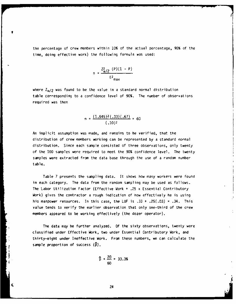
the percentage of crew members within 10% of the actual percentage, 90% of the

time, doing effective work) the following formula was used:

z a2 (P)(1 - P)

E2max

where Za/2 was found to be the value in a standard normal distribution

table corresponding to a confidence level of 90%. The number of observations

required was then

n = (1.645)2(.33)(.67) = 60

(.10)2

An implicit assumption was made, and remains to be verified, that the

distribution of crew members working can be represented by a standard normal

distribution. Since each sample consisted of three observations, only twenty

of the 100 samples were required to meet the 90% confidence level. The twenty

samples were extracted from the data base through the use of a random number

table.

Table 7 presents the sampling data. It shows how many workers were found

in each category. The data from the random sampling may be used as follows.

The Labor Utilization Factor (Effective Work + .25 x Essential Contributory

Work) gives the contractor a rough indication of how effectively he is using

his manpower resources. In this case, the LUF is .33 + .25(.03) = .34. This

value tends to verify the earlier observation that only one-third of the crew

members appeared to be working effectively (the dozer operator).

The data may be further analyzed. Of the sixty observations, twenty were

classified under Effective Work, two under Essential Contributory Work, and

thirty-eight under Ineffective Work. From these numbers, we can calculate the

sample proportion of success (s).

A 20p - - 33.3%

60

(24

Table 7. Sample data for fine-grading crew.

Work Number from Sub-Category Activity Sample Date Total Total %

Direct Work Grading w/Dozer 1111111111111111 16

20 33Operating 1111 4Scraper

Essential Measuring 1 1Contributory 2 3Work Holding String 1 1

Standing/Waiting 21222222222212 26

No Contact 111 3

Idle (Manned)Dozer

Ineffective Discussion Among 38 64Work Workers

Discussion w/ 111111 6Inspector

Idle (Manned)Scraper

Backing Dozer 3

25

The proportion of success in the population (p) (all recorded data sampled)

may be determined from the formula

A p 1I - P)P = p + Z=/

a c/2 n

established as 10%

P is found to be 33.3 ± 10%. We now have a confidence interval (C.I.) of 23.3

< p < 43.3 at a 90% confidence level. That is, 90% of the time, the actual

proportion of crew members doing effective work is between 23.3 and 43.3%.

If p is taken to be 33.3, a Frequency Histogram of Work Sampling Data

results from the following probability calculations.

The probability of finding no crew members doing effective work:

3! 0 3-0b(0; 3, 33.3) 3 (333) (.333) 3.7%

0! (3 - 0)!

The probability of finding one crew member doing effective work:

3! 1 3-1b(l; 3, 33.3) ! (.333) (.333) 11%

1! (3 - 1)!

The probability of finding two crew members doing effective work:

b(2; 3, 33.3) 3! (.333)2 3-2 11%2! (3 - 2)!

The probability of finding three crew members doing effective work:

b(3; 3, 33.3) 3! (.333) 3 (.333) 3 3.7%3! (3 - 3)!

26

Frequency Histogram of Work Sampling Data--where Number of Successes

is the number of crew members doing effective work.

U

.4

LA CoU T

UM

-o

L,.

Number of Successes

Looking at the data from a binominal standpoint, we can plot an Absolute

Frequency Polygon. Table 8 shows the data from the twenty samples divided

into two categories: Effective Work and Other.

Table 8. Work sampling data.

Sample Effective Sample EffectiveNumber Work Other Number Work Other

1 2 2 11 1 22 0 3 12 1 23 1 2 13 1 24 1 2 14 1 25 0 2 15 0 36 1 3 16 1 27 1 2 17 2 18 1 2 18 1 29 1 2 19 2 1

10 1 2 20 1 2

The data have a mean (T) of .95 with a standard deviation (a) of .51.

27

The Absolute Frequency Polygon shown below results.

9 /=M

39

e4-E °/ j

Lo I

*I.

Number of Men Working

The shape of the polygon suggests that the assumption that the sampled

data could be represented by a Standard Normal Distribution is correct.

All of this data manipulation is worth little if it does not lead to a

conclusion concerning the contractor's effectiveness in this particular

segment of the project. The on-site observation that only one of the three

crew members was working effectively, the calculated Labor Utilization Factor

of 34%, the Frequency Histogram which shows the probability of finding various

numbers of crew members working, and the Frequency Polygon which shows that,

in 15 of the 20 observations, only one crew member was working effectively,

all indicate a possible misuse of manpower resources by the contractor. The

party funding this operation finds Itself paying $3 for every $1 of effective

work. It is a recognized fact that not all work on a project contributes

directly to the accomplishment of the project, but must, nonetheless, be

28

performed. However, responsible management and supervision can, in many

cases, eliminate excessive wasted time. In this case, the crew member who

operated the scraper and held the string for the surveyor could have been

eliminated. The surveyor could have tied the string to the grade stakes at

each side of the track before checking elevations. Considering the infrequent

use of the scraper in this operation, and the proximity of the waste area to

the track, the dozer operator could have also operated the scraper without

significantly increasing the length of the job. The resultant savings, though

probably not a full one-third, would have been significant.

I

WORK SAMPLING STUDY OF PIPE-LAYING OPERATION

Ij

C|

WORK SAMPLING STUDY OF PIPE-LAYING OPERATION

A work sampling study was performed on the pipe-laying operation which

occurred on Thursday, 19 July. The operation involved digging a trench

approximately three feet in depth across a 35' wide section of clay track with

sloped shoulders. The cross-pipe, intended for the drainage of rain water

from the high side of the track to the low side, was to be installed at

approximately the 950' mark. Besides digging the trench, the three-man crew

had to shape the bottom of the trench to cradle the ten four-foot sections of

21" concrete pipe, compact the bottom of the trench with a gas-powered

compactor, bring the sections of pipe from the laydown area, set the sections

of pipe in the trench (ensuring proper joint and alignment), and backfill with

28 gravel. The crew had apparently been given one full day to complete the

task, and seemed to make every effort to ensure that a full day was required.

As with any work sampling study, work categories and activity

classifications were first established. Three categories were defined:

Effective Work--work directly related to the accomplishment of the task;

Essential Contributory Work--work performed to provide for the accomplishment

of the task, while not being directly related to it; and Ineffective Work--

activity, or inactivity, which did not lead to the accomplishment of the task.

Activities which were classified as Effective Work are: digging with the

backhoe or shovel, setting pipe into the trench, packing dirt around the side

of the pipe, operating the compactor, lifting pipe sections with the backhoe,

maneuvering the backhoe, cleaning dirt off the pipe ends to ensure proper

joint, and aligning pipe sections. Essential Contributory Work consisted of

measuring (checking the depth of the trench and the alignment of the pipe

sections), and attaching the pipe-hoist rig (either to the backhoe or to a

section of pipe). The activities classified as Ineffective Work were:

waiting (for an event to occur), no contact (absence from the work site),

break (short duration, sitting, relaxing, conversing with other crew members,

observing), and idleness (inactivity, regardless of reason).

A one and one-half hour observation time produced a data base of 145

samples. With each sample consisting of an observation of the activity of

0O 30

each of the three crew members, the result was a compilation of 435

observations.

During the recording segment, it appeared as though, at best, only one of

the three crew members was working effectively at any one time. Consequently,

a category proportion (p) of .33 was assumed. In order to determine the

number of observations required to yield a result satisfying a 90% Confidence

Level with Limit of Error of ± 10%, the following formula was used.

Z2 (P)( - P)n = a/2______

E2max

where Z,/2 was taken from areas under a Standard Normal Distribution.

The value of n was determined to be

n = (1.645)2(.33)(.67)_ = 60(.10)2

For the three-man crew, this meant that 20 samples were required. A random

number table was used to select the 20 samples. The results are shown in

Table 9.

The Labor Utilization Factor, a rough indication of how effectively the

contractor is using his manpower may be determined by adding the percentage of

Effective Work to 25% of the percentage of Essential Contributory Work. In

this case, LUF = .37 + .25(.03) = .38 (a low value).

Of the 60 observations in this data subset, 27 were classified as

Effective Work. The sample proportion of success (p) is then 27/60 or 45%

(higher than the assumed p of 33%). The calculated proportion of success in

the population (p) may now be found with the formula

A P (1 -P)

Sp Z a/2 n

established as 10%

31

Table 9. Sample data for pipe-laying crew.

Work Number from Sub-

Category Activity Sample Data Total Total %

Digging with Backhoe 1 1

Operating Compactor 1 1

Digging w/Shovel 2122 7

Lifting Pipe 1 1Effective 22 37Work Setting Pipe 12 3

Maneuvering Backhoe 111111111 9

Cleaning Pipe

Aligning Pipe

Packing Dirt AroundScale of Pipe

Essential Measuring 11 2ContributoryWork Attaching Pipe-Hoist 2 3

Rig

No Contact

Break 1122222222 32Ineffective 211111331 36 60Work

Idleness 112 4

Waiting

32-- . ----.- -.-.- 1

p is therefore 45 ± 10%. The confidence interval is 35 < p < 55 at a 90%

confidence level. What these numbers tell us is that, from the 60

observations analyzed, we can conclude that the percentage of crew members

working effectively on the operation is between 35% and 55%, 90% of the time.t

If p is taken to be 45, a Frequency Histogram results from the following

probability calculations.

The probability of finding no laborers doing effective work:

ii0 3-0b(O; 3, 45.0) 3! (.45) (.45) 9%0! (3 - 0)!

The probability of finding one laborer doing effective work:

3! 3-1b(1; 3, 45.0) 3! (.45) (.45) 27%

1! (3 - 1)!

The probability of finding two laborers doing effective work:

3! 2 3-2b(2; 3, 45.0) (.45) (.45) 27%

2! (3 - 2)!

The probability of finding three laborers doing effective work:

b(3; 3, 45.0) 3 (.45) 3 (.45)3 9%3! (3 - 3)!

33

4AI

I

.- *

U

Number of Successes

The Histogram indicates that the probability of finding none or three of

the crew members working is low, while the probability of finding one or two

of the crew members is higher (though not high-only 27%).

The data are now arranged and presented in a different manner. Table 10

shows the 60 observations arranged in two categories: Effective Work and

Other. The calculations yield an average of approximately one of the three

crew members doing effective work at any instant of observation. The Absolute

Frequency Polygon shows what has been tacitly assumed from the beginning, that

the distribution of data can be reasonably well represented by a standard

normal distribution.

The results of the analysis, though perhaps not entirely precise (a 90%

Confidence Level with a Limit of Error of t 10%), can lead to a few general

comments. It is obvious that there was a lot of "standing around" time. In

fact, during the observation period, when one crew member, reclined in the

seat of the backhoe, said "You guys let me know when it's time for a break,"

the responses from other crew members and an inspector were, "You've been on a

break since you got out here," and "Working at this pace, you guys don't need

a break." Reviewing the results of the analysis and the on-site impressions,

it appears that the job could have been performed 1) in half the time

allotted, or 2) by a smaller crew (2 men instead of 3).

I'

Table 10. Data set #1.

Sample Effective Sample EffectiveNumber Work Other Number Work Other

1 3 0 11 1 2t 2 2 1 12 1 2

3 1 2 13 1 24 1 2 14 2 15 1 2 15 0 36 1 2 16 2 17 1 2 17 2 18 1 2 18 0 39 1 2 19 0 310 1 2 20 0 3

39

C

(V

o o/

€c /

-3

cE

to-0--S4-)40

4AA

, Number of men .,. effective workL '4as-

35

-ilk . . .. .... ....... .

SUMMARY

The construction of the Truck Arrester Bed Research Facility, begun in

June, was completed in August 1984. Although the contractor's original

estimate of the time required was about four weeks, poor weather conditions

and competing manpower and equipment demands dragged out the project.

During the course of the project, a few instances were found in which it

appeared that manpower and time were being used somewhat inefficiently.

However, on a construction project, appearances can be deceiving. What seems

apparent in desk-top analyses is not always practical in the field. In any

event, the contractor's actions were well-executed and well-sequenced. The

contractor remained flexible and cooperative and altered his actions to suit

the needs of the Pennsylvania Transportation Institute, and offered several

suggestions to improve the quality of the final product. The result is a

well-constructed facility for research into the mechanism of stopping runaway

trucks.

r

36

-A. 6

I