RESEARCH PUBLICATION NO. 2/2017

DETERMINATION OF Z-R RELATIONSHIP AND

INUNDATION ANALYSIS FOR KUANTAN RIVER

BASIN

By Fauziana Ahmad, Tomoki Ushiyama, Takahiro Sayama

All rights reserved. No part of this publication may be reproduced in

any form, stored in a retrieval system, or transmitted in any form or

by any means electronic, mechanical, photocopying, recording or

otherwise without the prior written permission of the publisher.

Perpustakaan Negara Malaysia Cataloguing-in-Publication Data

Published and printed by

Jabatan Meteorologi Malaysia

Jalan Sultan

46667 PETALING JAYA

Selangor Darul Ehsan

Malaysia

Contents

No. Subject Page

Abstract

1. Introduction 1

2. Objective 5

3. Methodology

3.1 Radar Information and Hydrological

Characteristics

6

3.2 Data and Location Selected 8

3.3 Conversion of Radar Images into the

Quantitative Rainfall

3.4 Rainfall-Runoff Inundation (RRI) Model

10

11

4. Results and Discussions

4.1 Derivation of Z-R Relationship 12

4.2 RRI Model Output 29

5. Conclusions 37

References 39

Appendices 43

Determination of Z-R Relationship and Inundation Analysis for Kuantan River Basin

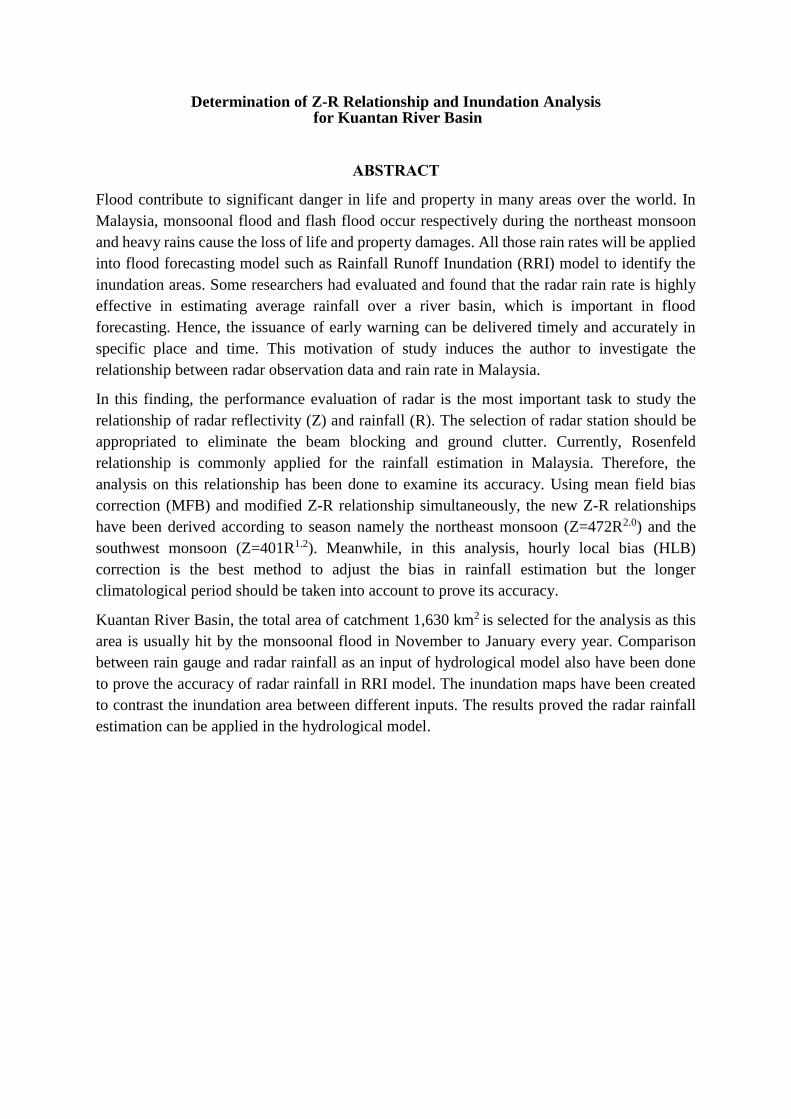
ABSTRACT

Flood contribute to significant danger in life and property in many areas over the world. In

Malaysia, monsoonal flood and flash flood occur respectively during the northeast monsoon

and heavy rains cause the loss of life and property damages. All those rain rates will be applied

into flood forecasting model such as Rainfall Runoff Inundation (RRI) model to identify the

inundation areas. Some researchers had evaluated and found that the radar rain rate is highly

effective in estimating average rainfall over a river basin, which is important in flood

forecasting. Hence, the issuance of early warning can be delivered timely and accurately in

specific place and time. This motivation of study induces the author to investigate the

relationship between radar observation data and rain rate in Malaysia.

In this finding, the performance evaluation of radar is the most important task to study the

relationship of radar reflectivity (Z) and rainfall (R). The selection of radar station should be

appropriated to eliminate the beam blocking and ground clutter. Currently, Rosenfeld

relationship is commonly applied for the rainfall estimation in Malaysia. Therefore, the

analysis on this relationship has been done to examine its accuracy. Using mean field bias

correction (MFB) and modified Z-R relationship simultaneously, the new Z-R relationships

have been derived according to season namely the northeast monsoon (Z=472R2.0) and the

southwest monsoon (Z=401R1.2). Meanwhile, in this analysis, hourly local bias (HLB)

correction is the best method to adjust the bias in rainfall estimation but the longer

climatological period should be taken into account to prove its accuracy.

Kuantan River Basin, the total area of catchment 1,630 km2 is selected for the analysis as this

area is usually hit by the monsoonal flood in November to January every year. Comparison

between rain gauge and radar rainfall as an input of hydrological model also have been done

to prove the accuracy of radar rainfall in RRI model. The inundation maps have been created

to contrast the inundation area between different inputs. The results proved the radar rainfall

estimation can be applied in the hydrological model.

1

1. INTRODUCTION

Malaysia is generally free from the severe natural disasters such as earthquakes, volcanic

eruptions and typhoons but it nonetheless not spared from other disasters such as flood, man-

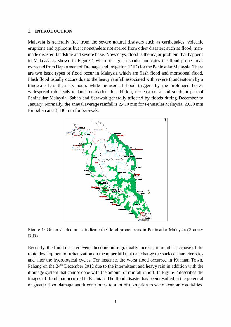
made disaster, landslide and severe haze. Nowadays, flood is the major problem that happens

in Malaysia as shown in Figure 1 where the green shaded indicates the flood prone areas

extracted from Department of Drainage and Irrigation (DID) for the Peninsular Malaysia. There

are two basic types of flood occur in Malaysia which are flash flood and monsoonal flood.

Flash flood usually occurs due to the heavy rainfall associated with severe thunderstorm by a

timescale less than six hours while monsoonal flood triggers by the prolonged heavy

widespread rain leads to land inundation. In addition, the east coast and southern part of

Peninsular Malaysia, Sabah and Sarawak generally affected by floods during December to

January. Normally, the annual average rainfall is 2,420 mm for Peninsular Malaysia, 2,630 mm

for Sabah and 3,830 mm for Sarawak.

Figure 1: Green shaded areas indicate the flood prone areas in Peninsular Malaysia (Source:

DID)

Recently, the flood disaster events become more gradually increase in number because of the

rapid development of urbanization on the upper hill that can change the surface characteristics

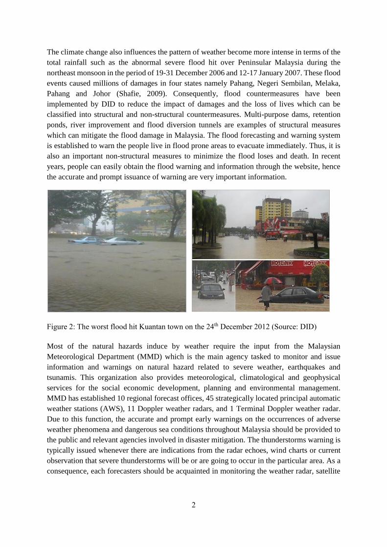
and alter the hydrological cycles. For instance, the worst flood occurred in Kuantan Town,

Pahang on the 24th December 2012 due to the intermittent and heavy rain in addition with the

drainage system that cannot cope with the amount of rainfall runoff. In Figure 2 describes the

images of flood that occurred in Kuantan. The flood disaster has been resulted in the potential

of greater flood damage and it contributes to a lot of disruption to socio economic activities.

2

The climate change also influences the pattern of weather become more intense in terms of the

total rainfall such as the abnormal severe flood hit over Peninsular Malaysia during the

northeast monsoon in the period of 19-31 December 2006 and 12-17 January 2007. These flood

events caused millions of damages in four states namely Pahang, Negeri Sembilan, Melaka,

Pahang and Johor (Shafie, 2009). Consequently, flood countermeasures have been

implemented by DID to reduce the impact of damages and the loss of lives which can be

classified into structural and non-structural countermeasures. Multi-purpose dams, retention

ponds, river improvement and flood diversion tunnels are examples of structural measures

which can mitigate the flood damage in Malaysia. The flood forecasting and warning system

is established to warn the people live in flood prone areas to evacuate immediately. Thus, it is

also an important non-structural measures to minimize the flood loses and death. In recent

years, people can easily obtain the flood warning and information through the website, hence

the accurate and prompt issuance of warning are very important information.

Figure 2: The worst flood hit Kuantan town on the 24th December 2012 (Source: DID)

Most of the natural hazards induce by weather require the input from the Malaysian

Meteorological Department (MMD) which is the main agency tasked to monitor and issue

information and warnings on natural hazard related to severe weather, earthquakes and

tsunamis. This organization also provides meteorological, climatological and geophysical

services for the social economic development, planning and environmental management.

MMD has established 10 regional forecast offices, 45 strategically located principal automatic

weather stations (AWS), 11 Doppler weather radars, and 1 Terminal Doppler weather radar.

Due to this function, the accurate and prompt early warnings on the occurrences of adverse

weather phenomena and dangerous sea conditions throughout Malaysia should be provided to

the public and relevant agencies involved in disaster mitigation. The thunderstorms warning is

typically issued whenever there are indications from the radar echoes, wind charts or current

observation that severe thunderstorms will be or are going to occur in the particular area. As a

consequence, each forecasters should be acquainted in monitoring the weather radar, satellite

3

images and forecast tools to provide the accurate and prompt warning for the public safety and

comfort.

The radar equation has already mentioned about the radar reflectivity factor which is a

meteorological parameter that is determined by the number and size of the particles present in

a sample volume. Due to the huge range of magnitudes (from 0.001 mm6/ m3 for fog, to

36,000,000 mm6/ m3 for softball-sized hail), the radar reflectivity is convenient to express in

decibels (dB) unit or dBZ as follows:-

𝑑𝐵𝑍 = 10 log10

𝑍

𝑚6 𝑚3⁄ (1)

where dBZ is the logarithmic radar reflectivity factor and Z is the linear radar reflectivity factor

in mm6/ m3. The relationship between rain rate (R) in unit mm/h and radar reflectivity factor

(Z) in unit 𝑚6 𝑚3⁄ is commonly described as empirical power-law relationship

𝑍 = 𝑎𝑅𝑏 (2)

where a and b are empirically derived constants. In reality, the radar reflectivity is measured

and used to calculate the rainrate, hence the equation (2) mostly appropriate written as

𝑅 = 𝐴𝑍𝐵 (3)

where A and B are again empirical constants. Many values are possible for both a and b

although b does not vary as much as a as described in Table 1.

Table 1: Several parameters a and b depend on the type of rainfall or cloud

Parameter a Parameter b Relationship Type of cloud

200 1.6 Marshall Palmer General stratiform precipitation

250 1.2 Rosenfeld Tropical convective system

400 1.4 Laws and Parsons General stratiform precipitation

300 1.5 Joss and Waldvogel General stratiform precipitation

Most commonly is the Marshall and Palmer relationship which is widely used to calculate the

rainfall amount. Typically, the values of a and b are classified according to the type of clouds.

Due to the different size of rain distributions, many researchers proposed the new derivation of

Z-R relationship and it is proved can be applied for rainfall estimation. Da Silva Moraes, et al.,

(2006) proposed several methods to set up the Z-R relationship such as disdrometer for

measuring a set of N(D). The derivation of Z-R relationship can be established by plotting Z

and R simultaneously and independently on log plot which a and b can be determined through

intercept and slope of the best-fit line. Reported values of a varies between 100 to 600, while

4

b varies between 1.3 to 1.8 (Haji Khamis, et al., 2005). They also mentioned if b is fixed at 1.6,

then a has an average of 360, 196 for continuous rain and 56 in drizzle.

Uijlenhoet (2001) illustrated that in the hydrological application, the conversion of radar

reflectivity factor Z to rain rate is the most crucial step since the accuracy of measurement and

prediction of spatial and temporal distribution rainfall are the most essential part in hydrology.

He added that the measurement of Z provides the best values when the radar has a perfect

calibration and the absence of attenuation, beam shielding and anomalous propagation.

L.S.Kumar, et al., (2011) studied about the reflectivity associated with the cloud rain type

which can be classified into convective, stratiform and transition types. In their analysis, they

found that convective stages have higher rain rate and higher reflectivity. Meanwhile using the

Atals-Ulbrich method, the values of a and b were varied from lower to higher in the convective

stage rather than in stratiform stages. In transition stages, the Z-R relationship was clearly

shown with lower a values and higher b value. This means that the Z-R relationship also

depends on type of rain classification. R.Suzana and T.Wardah (2011) analyzed the Z-R

relationship in Klang River Basin, Malaysia for exploring this kind of relationship by

classifying rainfall events into three different types (low, moderate and heavy). Using the

Marshall and Palmer relationship, they found the underestimation in the higher rainfall

intensities; hence the modification using new derivation of Z-R relationship yielded less error.

They emphasized that the Z-R relationship mostly depended on the location and type of rain as

the rain regimes were a very important parameter. R.Suzana, et al., (2011) in their discussion

about the Z-R relationship in Malaysia said that the analysis during different seasons gave less

errors compared to the Marshall and Palmer relationship using the optimization methods. They

also made a comparison with the new derivation relationship of rainfall type and found that the

errors minimized when using the seasonal relationship derivation.

M.Hunter (1996) also explained that a single calibration factor or bias can be applied to the

entire radar field using data from several rain gauge data. He, et al., (2011), Chumchean, et al.,

(2006) and A.Smith and F.Krajewski (1991) chose the mean field bias correction method which

is the simplest way to remove the bias between radar estimates at the rain gauge location and

the corresponding rain gauge amounts. They proposed the estimation of adjustment factor as

the ratio of accumulated rain gauge rainfall and the accumulated radar. They emphasized that

to obtain the accurate radar rainfall estimations are depending on the quality of radar signal

together with the best quality control. Hanchoowong, et al., (2012) reported that the bias

correction needs to be performed after errors in measured reflectivity and Z-R conversion errors

had been removed for instance, due to radial anomaly, errors caused by electronic problems

and none-signal rainfall. Typically, the initial radar rainfall estimations still remain their bias,

hence the bias adjustment factor should be established to reduce the errors.

5

2. OBJECTIVE

In this study, an analysis of Z-R relationship deployed in MMD and suggested new Z-R

relationship according to monsoon is developed. The study area is located in Kuantan River

Basin by utilizing Rainfall Runoff Inundation (RRI) model to identify the inundation area for

the early weather warning systems

A prompt and accurate flood forecasting and warning system can save lives and property in the

flood prone areas as well as assisting the authority in flood rescue operation. MMD is the main

agency tasked to monitor and issue information and warnings on natural hazard related to

severe weather. Therefore, the issuance of warnings which more focus on the location and time

is very important for the disaster mitigation in Malaysia. Each time, the meteorologists have to

refer the weather radar to know the propagations of rain cloud. This is essential to issue the

heavy rain or thunderstorms warnings to the general public and relevant agencies in disaster

mitigation. Radar observation is extremely useful to detect the properties of hydrometeor

systems in cloud which can be utilized as a forecasting tool.

The weather radar can be established as a tool for flood forecasting since it can provide critical

information in regions where the rain gauge information is unavailable. Basically, the

understandings of the physical factors of weather and radar limitation are essential for the

research of precipitation estimation. The new derivation of Z-R relationship depending on the

seasons will be developed for better comparison between the relationships that MMD currently

used. An analysis to prove the capabilities of the radar rainfall input is also needed in the flood

forecasting model as the issuance of warnings involve the specific area. As a result, the severe

weather warning will be issued more accurately and timely to make this department be the best

meteorological services. Therefore, this study is very useful to analyze the relationship between

radar observation data and rain rate, and applies the accurate radar rainfall estimation in

hydrological modeling since the precipitation is an essential part of the hydrological cycle.

6

3. METHODOLOGY

3.1 Radar Information and Hydrological Characteristics

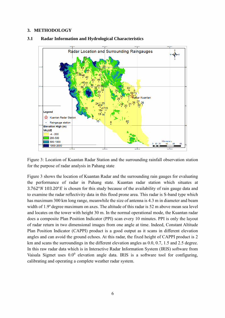
Figure 3: Location of Kuantan Radar Station and the surrounding rainfall observation station

for the purpose of radar analysis in Pahang state

Figure 3 shows the location of Kuantan Radar and the surrounding rain gauges for evaluating

the performance of radar in Pahang state. Kuantan radar station which situates at

3.762°𝑁 103.20°𝐸 is chosen for this study because of the availability of rain gauge data and

to examine the radar reflectivity data in this flood prone area. This radar is S-band type which

has maximum 300 km long range, meanwhile the size of antenna is 4.3 m in diameter and beam

width of 1.9o degree maximum on axes. The altitude of this radar is 52 m above mean sea level

and locates on the tower with height 30 m. In the normal operational mode, the Kuantan radar

does a composite Plan Position Indicator (PPI) scan every 10 minutes. PPI is only the layout

of radar return in two dimensional images from one angle at time. Indeed, Constant Altitude

Plan Position Indicator (CAPPI) product is a good output as it scans in different elevation

angles and can avoid the ground echoes. At this radar, the fixed height of CAPPI product is 2

km and scans the surroundings in the different elevation angles as 0.0, 0.7, 1.5 and 2.5 degree.

In this raw radar data which is in Interactive Radar Information System (IRIS) software from

Vaisala Sigmet uses 0.00 elevation angle data. IRIS is a software tool for configuring,

calibrating and operating a complete weather radar system.

7

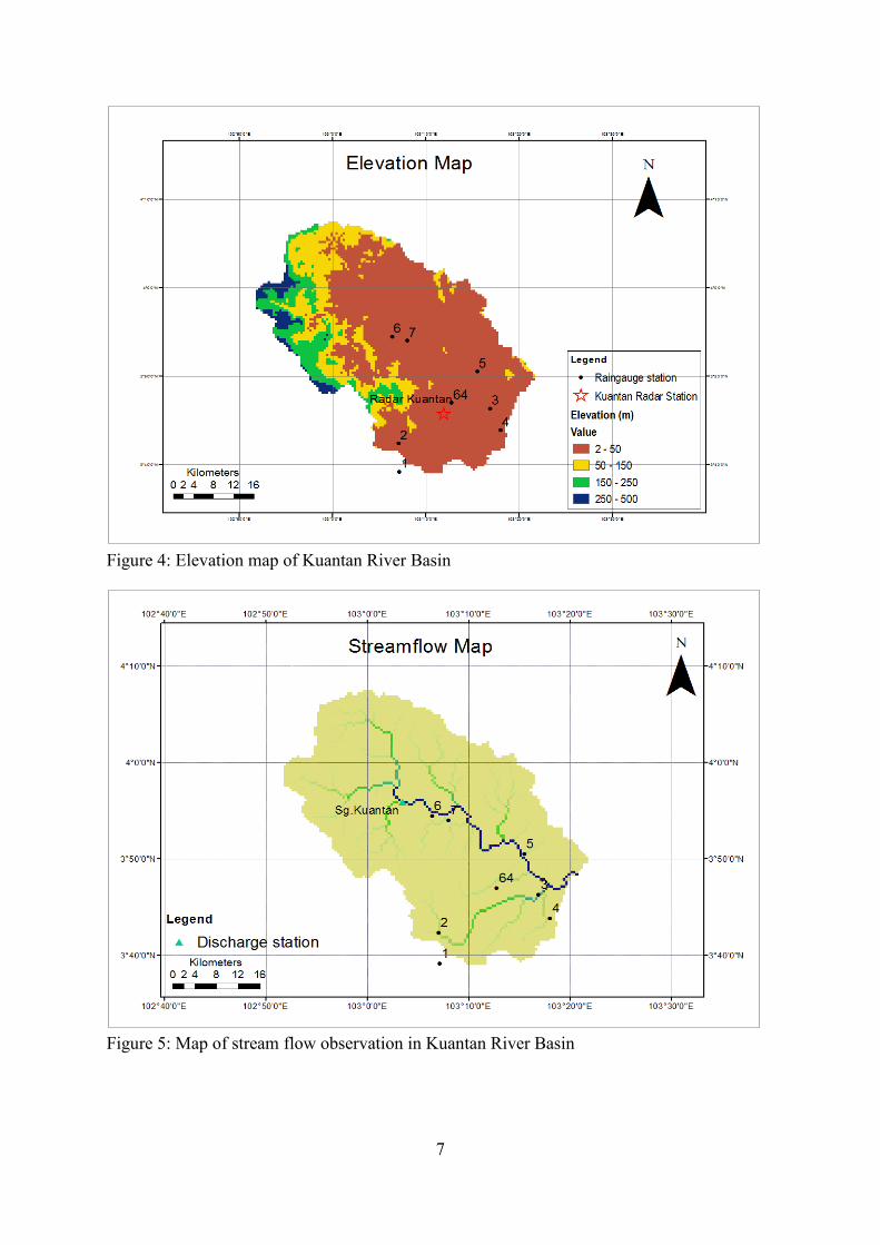
Figure 4: Elevation map of Kuantan River Basin

Figure 5: Map of stream flow observation in Kuantan River Basin

8

The Kuantan River Basin which is located at the eastern part of Peninsular Malaysia between

latitude 𝑁3.65° − 4.13° and longitude 𝐸102.86° − 103.37° as shown in Figure 4. Kuantan

River Basin is in the district of Kuantan at the northeastern end of Pahang state. It is one of the

important river basins in Pahang and has a total area of 1630 km2 which is started from forest

reserved area in Ulu Kuantan through Kuantan Town towards the South China Sea (Mohd

Nasir, et al., 2012). Figure 5 shows the map of stream flow observation station including the

river network in this basin. Kuantan River Basin consists of several important tributaries such

as Lembing River which located about 42 km northwest of Kuantan originated from Tapis

Mountain where the height is 1,520 m. All these rivers drain the major rural, agricultural, urban

and industrial areas of Kuantan district and discharge into the South China Sea. In term of land

use, forest and agriculture cover approximately 56% and 32% respectively from the whole area

of Kuantan District. Majority of the forested areas locate in the upstream of the basin. Kuantan

is the state capital of Pahang located near the mouth of Kuantan River and faces the South

China Sea. As 2010, the population of this district is 607,778 in total and this area is exposed

to the flood risk about three or four times in a year.

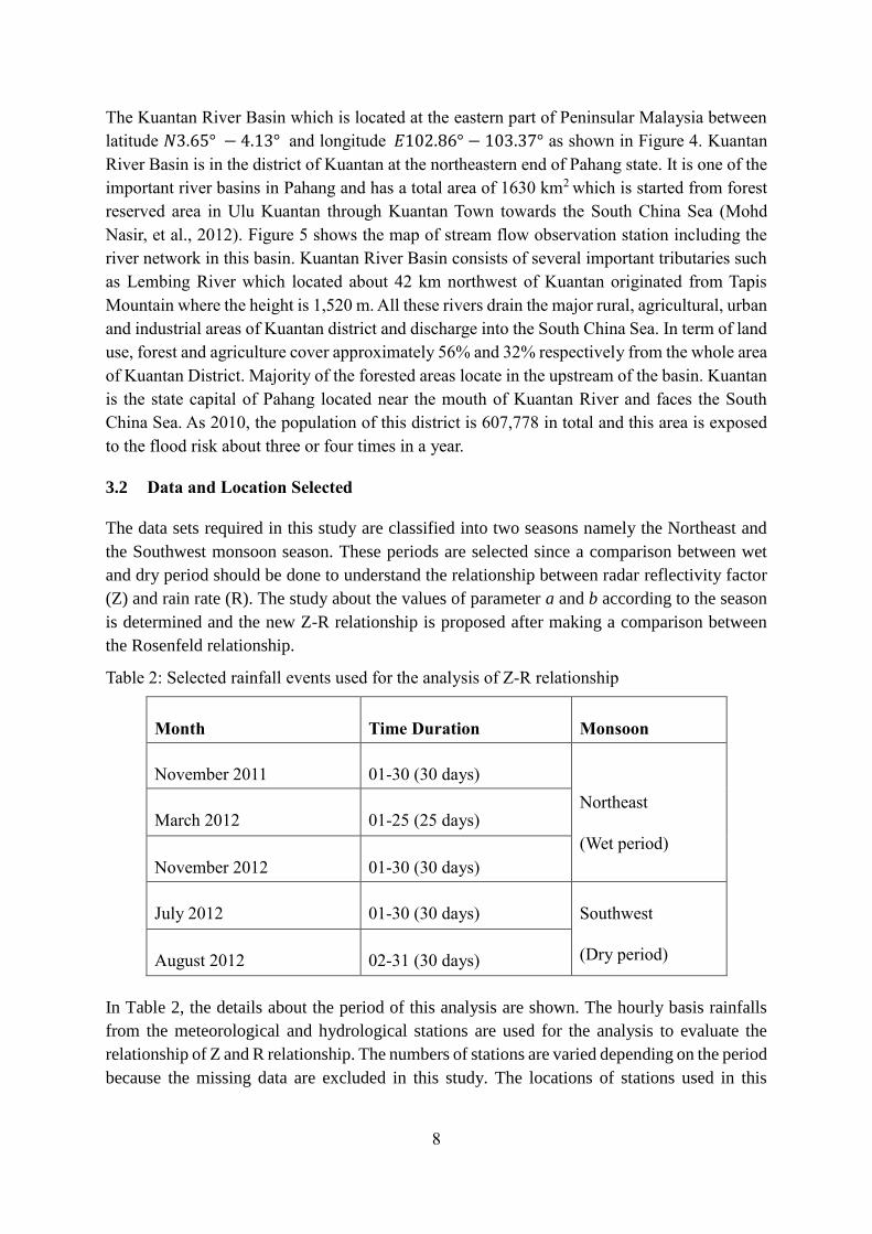
3.2 Data and Location Selected

The data sets required in this study are classified into two seasons namely the Northeast and

the Southwest monsoon season. These periods are selected since a comparison between wet

and dry period should be done to understand the relationship between radar reflectivity factor

(Z) and rain rate (R). The study about the values of parameter a and b according to the season

is determined and the new Z-R relationship is proposed after making a comparison between

the Rosenfeld relationship.

Table 2: Selected rainfall events used for the analysis of Z-R relationship

Month Time Duration Monsoon

November 2011 01-30 (30 days)

Northeast

(Wet period)

March 2012 01-25 (25 days)

November 2012 01-30 (30 days)

July 2012 01-30 (30 days) Southwest

(Dry period) August 2012 02-31 (30 days)

In Table 2, the details about the period of this analysis are shown. The hourly basis rainfalls

from the meteorological and hydrological stations are used for the analysis to evaluate the

relationship of Z and R relationship. The numbers of stations are varied depending on the period

because the missing data are excluded in this study. The locations of stations used in this

9

analysis are listed in Table 3. These rainfall data are used to compare the rainfall estimated

from radar with the observed values.

Table 3: List of rainfall observation stations in Pahang state

Name Station Latitude Longitude

3631001 1 3.653 103.119

3731018 2 3.706 103.117

3732020 3 3.772 103.281

3732021 4 3.731 103.3

3832015 5 3.842 103.258

48657 64 3.783 103.212

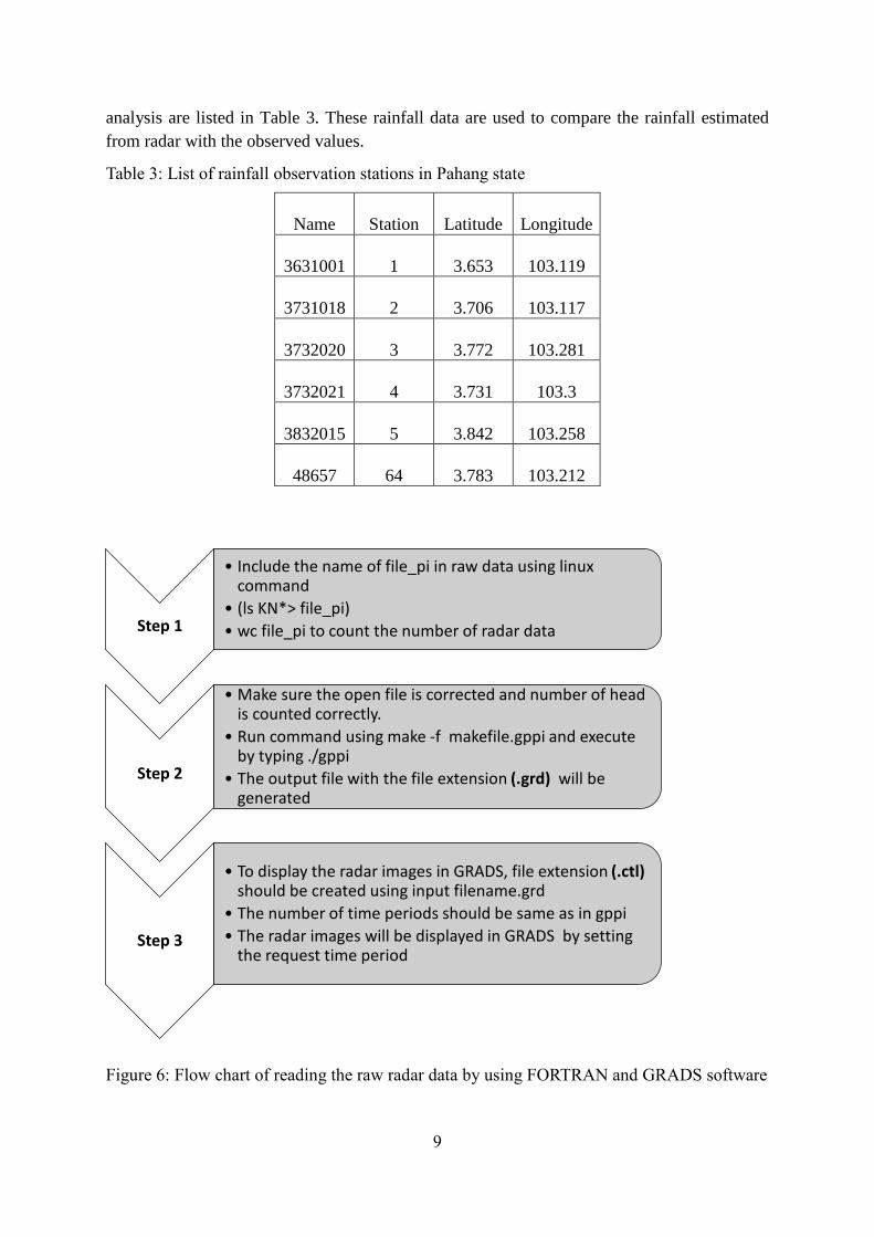
Figure 6: Flow chart of reading the raw radar data by using FORTRAN and GRADS software

Step 1

• Include the name of file_pi in raw data using linux command

• (ls KN*> file_pi)

• wc file_pi to count the number of radar data

Step 2

• Make sure the open file is corrected and number of head is counted correctly.

• Run command using make -f makefile.gppi and execute by typing ./gppi

• The output file with the file extension (.grd) will be generated

Step 3

• To display the radar images in GRADS, file extension (.ctl) should be created using input filename.grd

• The number of time periods should be same as in gppi

• The radar images will be displayed in GRADS by setting the request time period

10

The raw radar datasets are downloaded from MMD before converting the data into Grid

Analysis and Display System (GRADS) readable form. The following chart as in Figure 6 is

created for the further understanding in this conversion. A C program package to read the raw

data in Sigmet format was provided by Dr. M. Katsumata in JAMSTEC. This program is

combined with the FORTRAN programming to read the raw data and converted the original

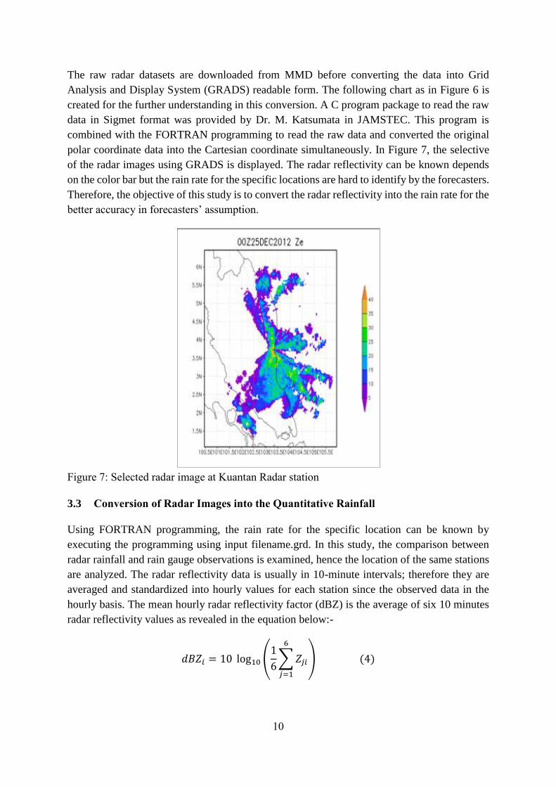
polar coordinate data into the Cartesian coordinate simultaneously. In Figure 7, the selective

of the radar images using GRADS is displayed. The radar reflectivity can be known depends

on the color bar but the rain rate for the specific locations are hard to identify by the forecasters.

Therefore, the objective of this study is to convert the radar reflectivity into the rain rate for the

better accuracy in forecasters’ assumption.

Figure 7: Selected radar image at Kuantan Radar station

3.3 Conversion of Radar Images into the Quantitative Rainfall

Using FORTRAN programming, the rain rate for the specific location can be known by

executing the programming using input filename.grd. In this study, the comparison between

radar rainfall and rain gauge observations is examined, hence the location of the same stations

are analyzed. The radar reflectivity data is usually in 10-minute intervals; therefore they are

averaged and standardized into hourly values for each station since the observed data in the

hourly basis. The mean hourly radar reflectivity factor (dBZ) is the average of six 10 minutes

radar reflectivity values as revealed in the equation below:-

𝑑𝐵𝑍𝑖 = 10 log10 (1

6∑ 𝑍𝑗𝑖

6

𝑗=1

) (4)

11

where 𝑑𝐵𝑍𝑖 is the mean radar reflectivity factor for the i hour and 𝑍𝑗𝑖 is radar reflectivity for

the j-th minute observation at the i-th hour and i (= 1, 2, 3,….). The radar reflectivity is used in

decibel unit for the easier understanding estimation of rainfall intensity. As shown in Figure 7,

the lowest value in purple color (0<dBZ<5) indicates the shallow reflectivity (light rainfall)

meanwhile the highest value in orange color (dBZ>40) shows the highest reflectivity factor

(heavy rainfall). This is concluded that the colors are reflected to the different echo intensities

measured in dBZ during each elevation scan.

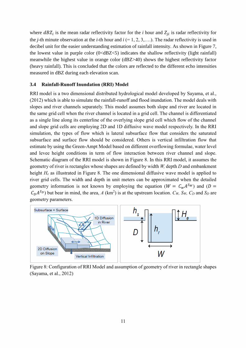
3.4 Rainfall-Runoff Inundation (RRI) Model

RRI model is a two dimensional distributed hydrological model developed by Sayama, et al.,

(2012) which is able to simulate the rainfall-runoff and flood inundation. The model deals with

slopes and river channels separately. This model assumes both slope and river are located in

the same grid cell when the river channel is located in a grid cell. The channel is differentiated

as a single line along its centerline of the overlying slope grid cell which flow of the channel

and slope grid cells are employing 2D and 1D diffusive wave model respectively. In the RRI

simulation, the types of flow which is lateral subsurface flow that considers the saturated

subsurface and surface flow should be considered. Others is vertical infiltration flow that

estimate by using the Green-Ampt Model based on different overflowing formulae, water level

and levee height conditions in term of flow interaction between river channel and slope.

Schematic diagram of the RRI model is shown in Figure 8. In this RRI model, it assumes the

geometry of river is rectangles whose shapes are defined by width W, depth D and embankment

height He as illustrated in Figure 8. The one dimensional diffusive wave model is applied to

river grid cells. The width and depth in unit meters can be approximated when the detailed

geometry information is not known by employing the equation (𝑊 = 𝐶𝑤𝐴𝑆𝑊) and (𝐷 =

𝐶𝐷𝐴𝑆𝐷) but bear in mind, the area, A (km2) is at the upstream location. CW, SW, CD and SD are

geometry parameters.

Figure 8: Configuration of RRI Model and assumption of geometry of river in rectangle shapes

(Sayama, et al., 2012)

12

4. RESULTS AND DISCUSSION

4.1 Derivation of Z-R Relationship

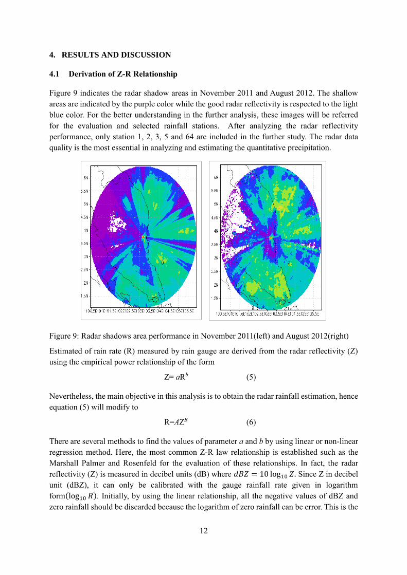
Figure 9 indicates the radar shadow areas in November 2011 and August 2012. The shallow

areas are indicated by the purple color while the good radar reflectivity is respected to the light

blue color. For the better understanding in the further analysis, these images will be referred

for the evaluation and selected rainfall stations. After analyzing the radar reflectivity

performance, only station 1, 2, 3, 5 and 64 are included in the further study. The radar data

quality is the most essential in analyzing and estimating the quantitative precipitation.

Figure 9: Radar shadows area performance in November 2011(left) and August 2012(right)

Estimated of rain rate (R) measured by rain gauge are derived from the radar reflectivity (Z)

using the empirical power relationship of the form

Z= aRb (5)

Nevertheless, the main objective in this analysis is to obtain the radar rainfall estimation, hence

equation (5) will modify to

R=AZB (6)

There are several methods to find the values of parameter a and b by using linear or non-linear

regression method. Here, the most common Z-R law relationship is established such as the

Marshall Palmer and Rosenfeld for the evaluation of these relationships. In fact, the radar

reflectivity (Z) is measured in decibel units (dB) where 𝑑𝐵𝑍 = 10 log10 𝑍. Since Z in decibel

unit (dBZ), it can only be calibrated with the gauge rainfall rate given in logarithm

form(log10 𝑅). Initially, by using the linear relationship, all the negative values of dBZ and

zero rainfall should be discarded because the logarithm of zero rainfall can be error. This is the

13

purpose the radar data between dBZ > 0 and R> 0 is selected. Furthermore, the dBZ data less

than 15 and greater than 53 are excluded in this analysis to avoid the effect of noise and high

reflectivity cause by the contamination from hail (Hanchoowong, et al., 2012).

Using linear regression method, parameter a and b is obtained by fitting the linear relationship

between dBZ and log10 𝑅 by the use of equation as below:-

log10 𝑅 = 10𝐵 log10 𝑍 + log10 𝐴 (7)

Corresponding to a straight line function (best-fit) that obtains 𝑦 = 𝑚𝑥 + 𝑐 where y = log10 𝑅,

m is the slope, x = dBZ and c is the y-axis intercept, the new Z-R relationship is obtained. The

coefficients, a and b in are estimated from equation as follows:-

𝑅 = (𝑍

𝑎)

1𝑏

(8)

Meanwhile, non-linear least square (nls) command is used in R programming for the non-linear

regression method by using same radar data used. After including the good radar reflectivity,

the comparisons between these both of methods including the Rosenfeld relationship are

examined for a better comparison. Thus, the method and radar data used for the analysis after

excluding the low radar reflectivity are examined again as shown in Table 4 by using March

2012 rainfall event.

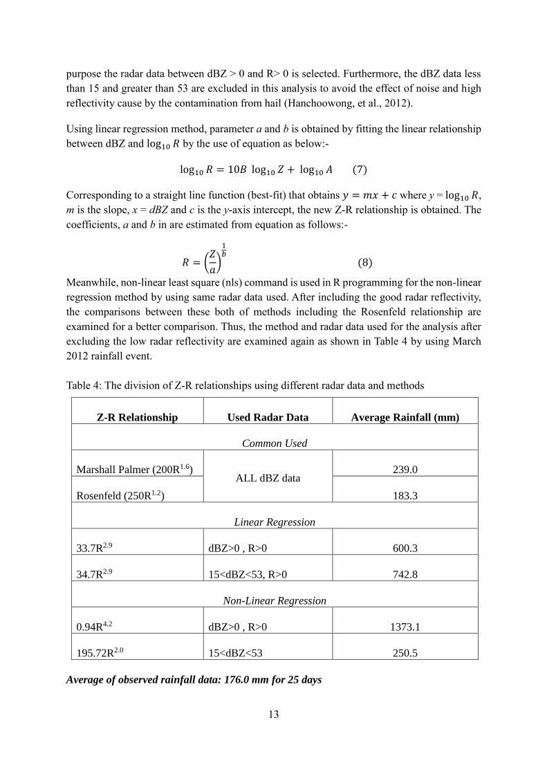
Table 4: The division of Z-R relationships using different radar data and methods

Z-R Relationship Used Radar Data Average Rainfall (mm)

Common Used

Marshall Palmer (200R1.6) ALL dBZ data

239.0

Rosenfeld (250R1.2) 183.3

Linear Regression

33.7R2.9 dBZ>0 , R>0 600.3

34.7R2.9 15<dBZ<53, R>0 742.8

Non-Linear Regression

0.94R4.2 dBZ>0 , R>0 1373.1

195.72R2.0 15<dBZ<53 250.5

Average of observed rainfall data: 176.0 mm for 25 days

14

Table 5: Statistical analyses for each Z-R relationship

Statistical

Measurement 200R1.6 250R1.2 33.7R2.9 34.7R2.9 0.94R4.2 195.72R2.0

RMSE 1.64 1.76 1.76 1.76 2.59 1.62

Total Error 0.36 0.04 2.41 2.38 6.81 0.43

BIAS (%) 35.9 4.22 241.34 237.92 680.86 42.45

In Table 5, the Rosenfeld rainfall estimations are seem accurate compare to the subsequent

methods as they gives the lowest value of total error since the total error equal to zero is the

best results. When the comparison between all of these relationships is done, 𝑍 = 250𝑅1.2

presents the small percent of bias, but 𝑍 = 195.72𝑅2.0 still gives the smallest Root Mean

Square Error (RMSE). It is proved that the best method to apply for the derivation of Z-R

relationship is by non-linear regression method along with 15<dBZ<53. The Rosenfeld

relationship is remained for the further analysis to compare with the rainfall estimation after

the rainfall adjustment.

This study is focused to remove the bias in radar rainfall estimates rather than removing all

systematic error. Consequently, the adjustment factor using mean field bias correction (MFB)

is the simplest method which this bias correction factor is constant over time and space

(Hanchoowong, et al., 2012). MFB (F) can be calculated as follows:-

𝐹 =∑ 𝐺𝑖𝑛

𝑖=1

∑ 𝑅𝑖𝑛𝑖=1

(9)

where Gi is the accumulation of observed rainfall divided with the accumulation of initial radar

rainfall estimation in multiple station n for the whole periods of calibration. This statistical

approach is straight forward, effective and widely used by the researchers in the radar rainfall

estimations.

Using the formula of MFB, the equation of (5) is modified into the new equation which can be

written as

𝑍 = 𝑎𝐹−𝑏𝑅𝑏 (10)

where a and b are constant parameters derived from the initial radar rainfall estimates. This

new equation is created because of the multiplication of the adjustment factor (F) to the initial

radar rainfall estimates. To make it simple way, this factor is multiplied with the parameter a

to get the new value of a until the smallest bias in the final output which mostly the total error

should be zero to obtain the best results. In this case, the value of b is not change as

(Hanchoowong, et al., 2012) said that the parameter b is not influence RMSE so much in the

radar rainfall estimation.

15

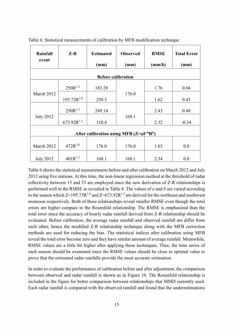
Table 6: Statistical measurements of calibration by MFB modification technique

Rainfall

event

Z-R

Estimated

(mm)

Observed

(mm)

RMSE

(mm/h)

Total Error

(mm)

Before calibration

March 2012

250R1.2 183.28

176.0

1.76 0.04

195.72R2.0 250.5 1.62 0.43

July 2012

250R1.2 249.14

168.1

2.43 0.48

673.92R1.2 110.4 2.32 -0.34

After calibration using MFB (Z=aF-bRb)

March 2012 472R2.0 176.0 176.0 1.63 0.0

July 2012 401R1.2 168.1 168.1 2.34 0.0

Table 6 shows the statistical measurements before and after calibration on March 2012 and July

2012 using five stations. At this time, the non-linear regression method at the threshold of radar

reflectivity between 15 and 53 are employed since the new derivation of Z-R relationships is

performed well in the RMSE as revealed in Table 4. The values of a and b are varied according

to the season which Z=195.75R2.0 and Z=673.92R1.2 are derived for the northeast and southwest

monsoon respectively. Both of these relationships reveal smaller RMSE even though the total

errors are higher compare to the Rosenfeld relationship. The RMSE is emphasized than the

total error since the accuracy of hourly radar rainfall derived from Z-R relationship should be

evaluated. Before calibration, the average radar rainfall and observed rainfall are differ from

each other, hence the modified Z-R relationship technique along with the MFB correction

methods are used for reducing the bias. The statistical indices after calibration using MFB

reveal the total error become zero and they have similar amount of average rainfall. Meanwhile,

RMSE values are a little bit higher after applying those techniques. Thus, the time series of

each season should be examined since the RMSE values should be close to optimal value to

prove that the estimated radar rainfalls provide the most accurate estimation.

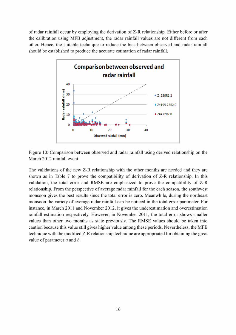
In order to evaluate the performance of calibration before and after adjustment, the comparison

between observed and radar rainfall is shown as in Figure 10. The Rosenfeld relationship is

included in the figure for better comparison between relationships that MMD currently used.

Each radar rainfall is compared with the observed rainfall and found that the underestimations

16

of radar rainfall occur by employing the derivation of Z-R relationship. Either before or after

the calibration using MFB adjustment, the radar rainfall values are not different from each

other. Hence, the suitable technique to reduce the bias between observed and radar rainfall

should be established to produce the accurate estimation of radar rainfall.

Figure 10: Comparison between observed and radar rainfall using derived relationship on the

March 2012 rainfall event

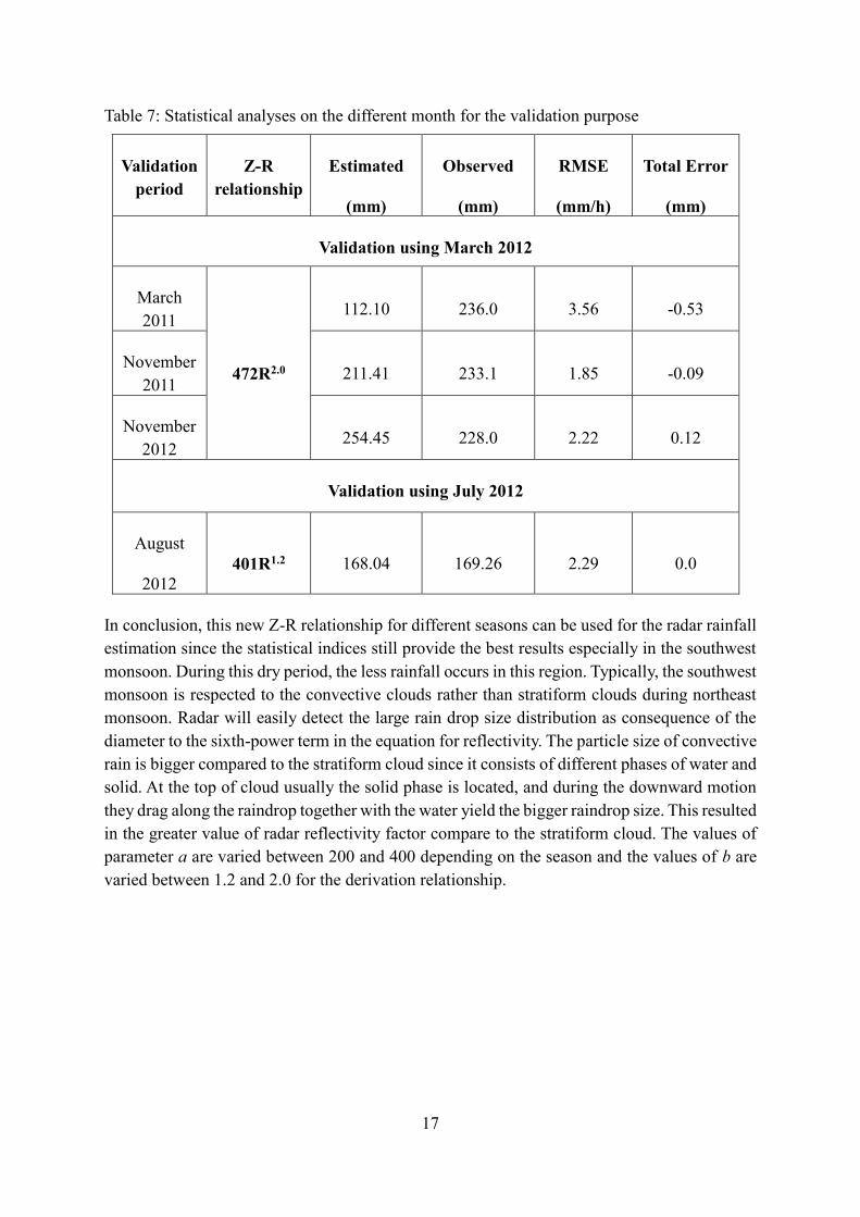
The validations of the new Z-R relationship with the other months are needed and they are

shown as in Table 7 to prove the compatibility of derivation of Z-R relationship. In this

validation, the total error and RMSE are emphasized to prove the compatibility of Z-R

relationship. From the perspective of average radar rainfall for the each season, the southwest

monsoon gives the best results since the total error is zero. Meanwhile, during the northeast

monsoon the variety of average radar rainfall can be noticed in the total error parameter. For

instance, in March 2011 and November 2012, it gives the underestimation and overestimation

rainfall estimation respectively. However, in November 2011, the total error shows smaller

values than other two months as state previously. The RMSE values should be taken into

caution because this value still gives higher value among these periods. Nevertheless, the MFB

technique with the modified Z-R relationship technique are appropriated for obtaining the great

value of parameter a and b.

17

Table 7: Statistical analyses on the different month for the validation purpose

Validation

period

Z-R

relationship

Estimated

(mm)

Observed

(mm)

RMSE

(mm/h)

Total Error

(mm)

Validation using March 2012

March

2011

472R2.0

112.10 236.0 3.56 -0.53

November

2011 211.41 233.1 1.85 -0.09

November

2012 254.45 228.0 2.22 0.12

Validation using July 2012

August

2012

401R1.2 168.04 169.26 2.29 0.0

In conclusion, this new Z-R relationship for different seasons can be used for the radar rainfall

estimation since the statistical indices still provide the best results especially in the southwest

monsoon. During this dry period, the less rainfall occurs in this region. Typically, the southwest

monsoon is respected to the convective clouds rather than stratiform clouds during northeast

monsoon. Radar will easily detect the large rain drop size distribution as consequence of the

diameter to the sixth-power term in the equation for reflectivity. The particle size of convective

rain is bigger compared to the stratiform cloud since it consists of different phases of water and

solid. At the top of cloud usually the solid phase is located, and during the downward motion

they drag along the raindrop together with the water yield the bigger raindrop size. This resulted

in the greater value of radar reflectivity factor compare to the stratiform cloud. The values of

parameter a are varied between 200 and 400 depending on the season and the values of b are

varied between 1.2 and 2.0 for the derivation relationship.

18

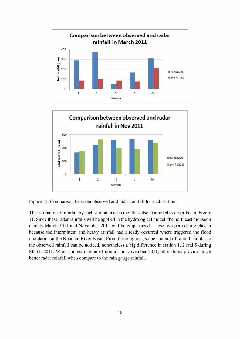
Figure 11: Comparison between observed and radar rainfall for each station

The estimation of rainfall by each station in each month is also examined as described in Figure

11. Since these radar rainfalls will be applied in the hydrological model, the northeast monsoon

namely March 2011 and November 2011 will be emphasized. These two periods are chosen

because the intermittent and heavy rainfall had already occurred where triggered the flood

inundation at the Kuantan River Basin. From these figures, some amount of rainfall similar to

the observed rainfall can be noticed, nonetheless a big difference in station 1, 2 and 5 during

March 2011. Whilst, in estimation of rainfall in November 2011, all stations provide much

better radar rainfall when compare to the rain gauge rainfall.

19

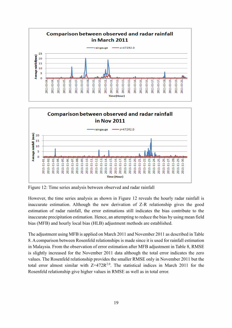
Figure 12: Time series analysis between observed and radar rainfall

However, the time series analysis as shown in Figure 12 reveals the hourly radar rainfall is

inaccurate estimation. Although the new derivation of Z-R relationship gives the good

estimation of radar rainfall, the error estimations still indicates the bias contribute to the

inaccurate precipitation estimation. Hence, an attempting to reduce the bias by using mean field

bias (MFB) and hourly local bias (HLB) adjustment methods are established.

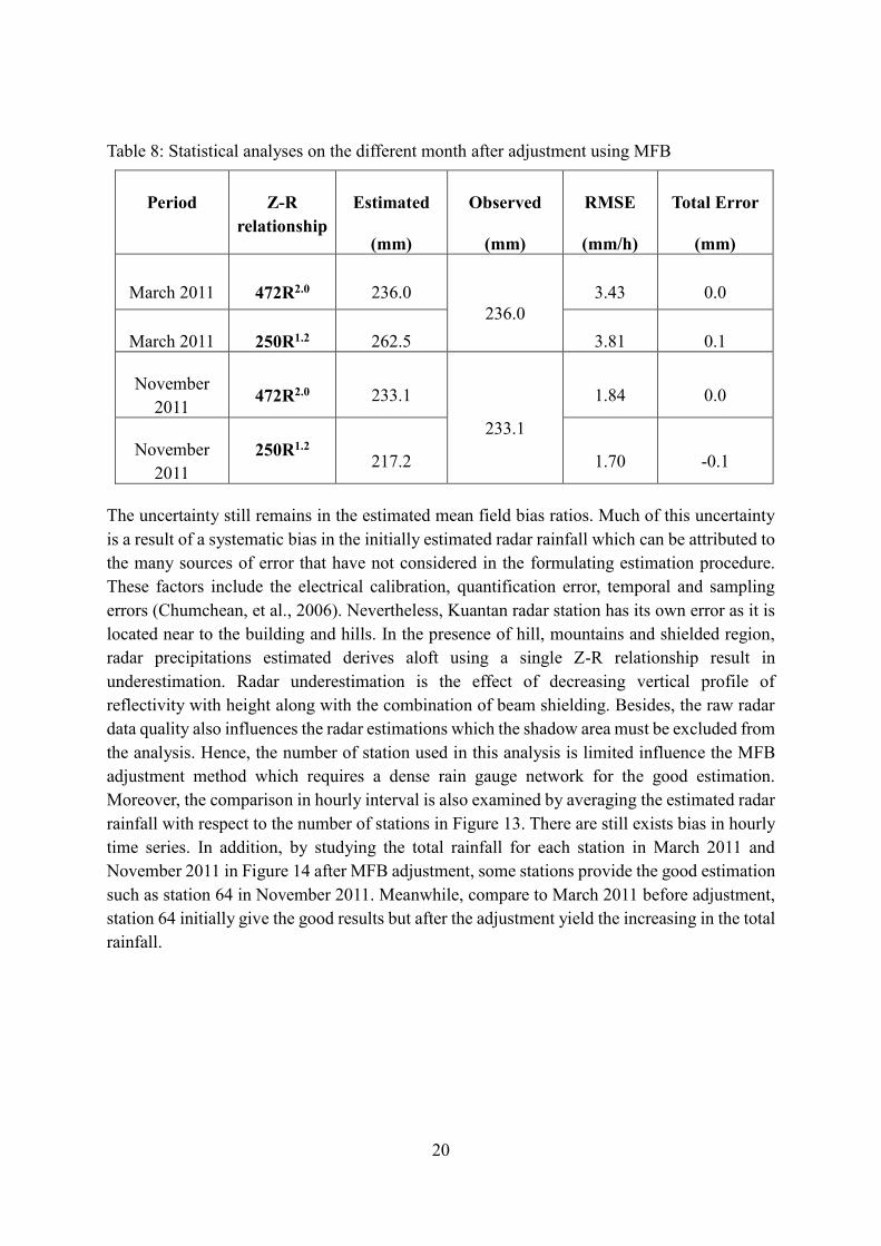
The adjustment using MFB is applied on March 2011 and November 2011 as described in Table

8. A comparison between Rosenfeld relationships is made since it is used for rainfall estimation

in Malaysia. From the observation of error estimation after MFB adjustment in Table 8, RMSE

is slightly increased for the November 2011 data although the total error indicates the zero

values. The Rosenfeld relationship provides the smaller RMSE only in November 2011 but the

total error almost similar with Z=472R2.0. The statistical indices in March 2011 for the

Rosenfeld relationship give higher values in RMSE as well as in total error.

20

Table 8: Statistical analyses on the different month after adjustment using MFB

Period Z-R

relationship

Estimated

(mm)

Observed

(mm)

RMSE

(mm/h)

Total Error

(mm)

March 2011 472R2.0 236.0

236.0

3.43 0.0

March 2011 250R1.2 262.5 3.81 0.1

November

2011 472R2.0 233.1

233.1

1.84 0.0

November

2011

250R1.2 217.2 1.70 -0.1

The uncertainty still remains in the estimated mean field bias ratios. Much of this uncertainty

is a result of a systematic bias in the initially estimated radar rainfall which can be attributed to

the many sources of error that have not considered in the formulating estimation procedure.

These factors include the electrical calibration, quantification error, temporal and sampling

errors (Chumchean, et al., 2006). Nevertheless, Kuantan radar station has its own error as it is

located near to the building and hills. In the presence of hill, mountains and shielded region,

radar precipitations estimated derives aloft using a single Z-R relationship result in

underestimation. Radar underestimation is the effect of decreasing vertical profile of

reflectivity with height along with the combination of beam shielding. Besides, the raw radar

data quality also influences the radar estimations which the shadow area must be excluded from

the analysis. Hence, the number of station used in this analysis is limited influence the MFB

adjustment method which requires a dense rain gauge network for the good estimation.

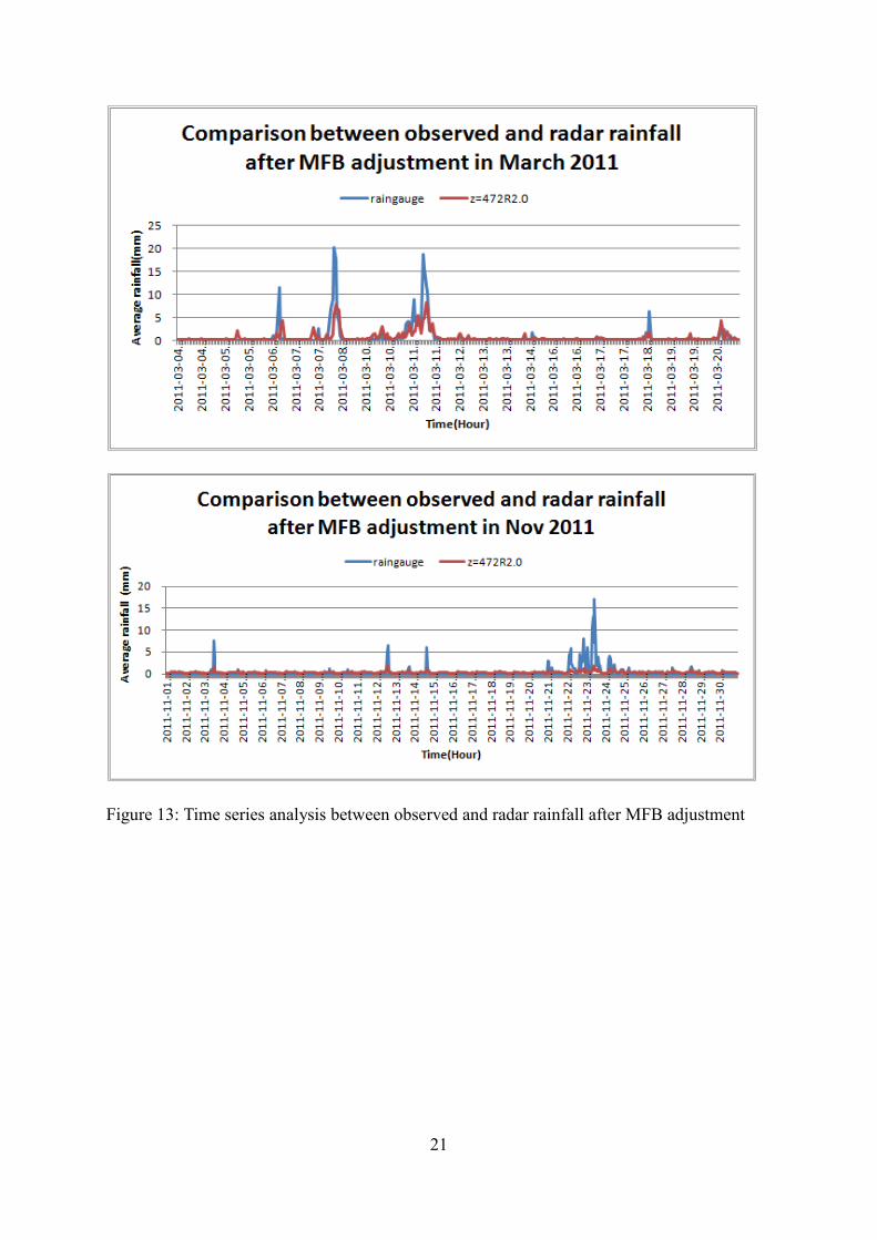
Moreover, the comparison in hourly interval is also examined by averaging the estimated radar

rainfall with respect to the number of stations in Figure 13. There are still exists bias in hourly

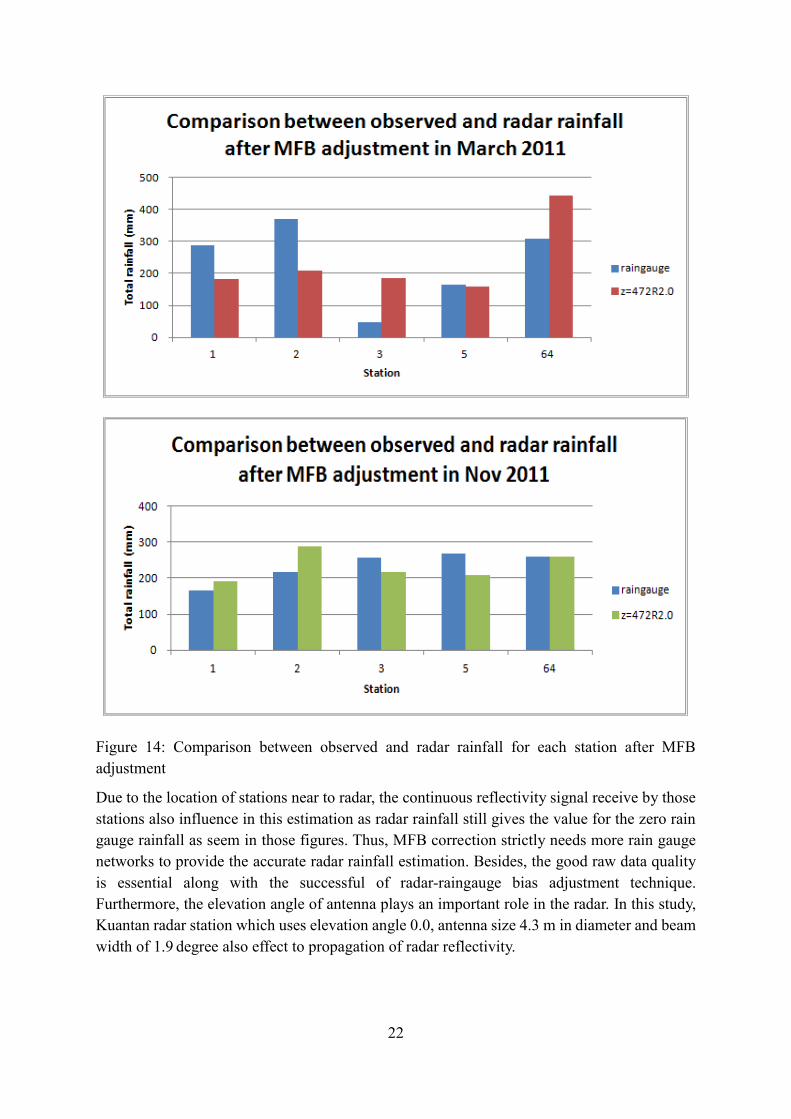
time series. In addition, by studying the total rainfall for each station in March 2011 and

November 2011 in Figure 14 after MFB adjustment, some stations provide the good estimation

such as station 64 in November 2011. Meanwhile, compare to March 2011 before adjustment,

station 64 initially give the good results but after the adjustment yield the increasing in the total

rainfall.

21

Figure 13: Time series analysis between observed and radar rainfall after MFB adjustment

22

Figure 14: Comparison between observed and radar rainfall for each station after MFB

adjustment

Due to the location of stations near to radar, the continuous reflectivity signal receive by those

stations also influence in this estimation as radar rainfall still gives the value for the zero rain

gauge rainfall as seem in those figures. Thus, MFB correction strictly needs more rain gauge

networks to provide the accurate radar rainfall estimation. Besides, the good raw data quality

is essential along with the successful of radar-raingauge bias adjustment technique.

Furthermore, the elevation angle of antenna plays an important role in the radar. In this study,

Kuantan radar station which uses elevation angle 0.0, antenna size 4.3 m in diameter and beam

width of 1.9 degree also effect to propagation of radar reflectivity.

23

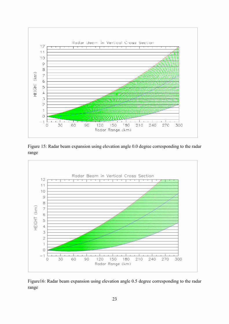
Figure 15: Radar beam expansion using elevation angle 0.0 degree corresponding to the radar

range

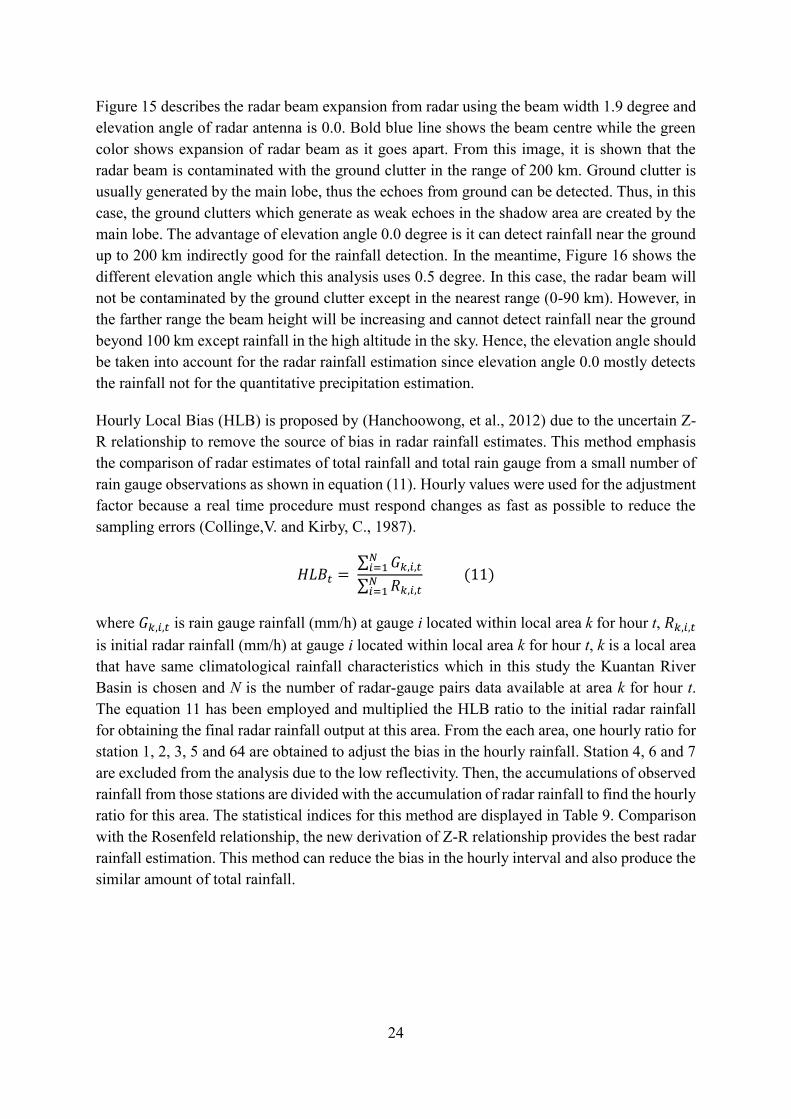
Figure16: Radar beam expansion using elevation angle 0.5 degree corresponding to the radar

range

24

Figure 15 describes the radar beam expansion from radar using the beam width 1.9 degree and

elevation angle of radar antenna is 0.0. Bold blue line shows the beam centre while the green

color shows expansion of radar beam as it goes apart. From this image, it is shown that the

radar beam is contaminated with the ground clutter in the range of 200 km. Ground clutter is

usually generated by the main lobe, thus the echoes from ground can be detected. Thus, in this

case, the ground clutters which generate as weak echoes in the shadow area are created by the

main lobe. The advantage of elevation angle 0.0 degree is it can detect rainfall near the ground

up to 200 km indirectly good for the rainfall detection. In the meantime, Figure 16 shows the

different elevation angle which this analysis uses 0.5 degree. In this case, the radar beam will

not be contaminated by the ground clutter except in the nearest range (0-90 km). However, in

the farther range the beam height will be increasing and cannot detect rainfall near the ground

beyond 100 km except rainfall in the high altitude in the sky. Hence, the elevation angle should

be taken into account for the radar rainfall estimation since elevation angle 0.0 mostly detects

the rainfall not for the quantitative precipitation estimation.

Hourly Local Bias (HLB) is proposed by (Hanchoowong, et al., 2012) due to the uncertain Z-

R relationship to remove the source of bias in radar rainfall estimates. This method emphasis

the comparison of radar estimates of total rainfall and total rain gauge from a small number of

rain gauge observations as shown in equation (11). Hourly values were used for the adjustment

factor because a real time procedure must respond changes as fast as possible to reduce the

sampling errors (Collinge,V. and Kirby, C., 1987).

𝐻𝐿𝐵𝑡 = ∑ 𝐺𝑘,𝑖,𝑡

𝑁𝑖=1

∑ 𝑅𝑘,𝑖,𝑡𝑁𝑖=1

(11)

where 𝐺𝑘,𝑖,𝑡 is rain gauge rainfall (mm/h) at gauge i located within local area k for hour t, 𝑅𝑘,𝑖,𝑡

is initial radar rainfall (mm/h) at gauge i located within local area k for hour t, k is a local area

that have same climatological rainfall characteristics which in this study the Kuantan River

Basin is chosen and N is the number of radar-gauge pairs data available at area k for hour t.

The equation 11 has been employed and multiplied the HLB ratio to the initial radar rainfall

for obtaining the final radar rainfall output at this area. From the each area, one hourly ratio for

station 1, 2, 3, 5 and 64 are obtained to adjust the bias in the hourly rainfall. Station 4, 6 and 7

are excluded from the analysis due to the low reflectivity. Then, the accumulations of observed

rainfall from those stations are divided with the accumulation of radar rainfall to find the hourly

ratio for this area. The statistical indices for this method are displayed in Table 9. Comparison

with the Rosenfeld relationship, the new derivation of Z-R relationship provides the best radar

rainfall estimation. This method can reduce the bias in the hourly interval and also produce the

similar amount of total rainfall.

25

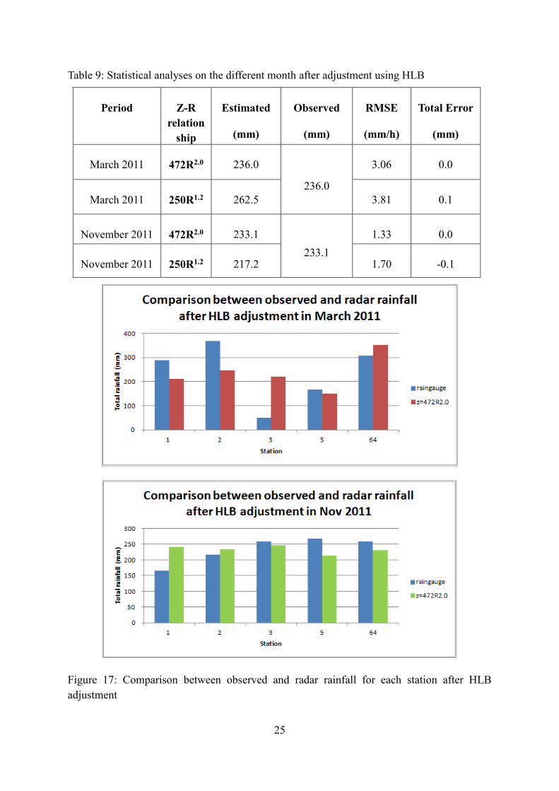
Table 9: Statistical analyses on the different month after adjustment using HLB

Period Z-R

relation

ship

Estimated

(mm)

Observed

(mm)

RMSE

(mm/h)

Total Error

(mm)

March 2011 472R2.0 236.0

236.0

3.06 0.0

March 2011 250R1.2 262.5 3.81 0.1

November 2011 472R2.0 233.1

233.1

1.33 0.0

November 2011 250R1.2 217.2 1.70 -0.1

Figure 17: Comparison between observed and radar rainfall for each station after HLB

adjustment

26

The analyses of each station are described for November 2011 and March 2011 as shown in

Figure 17. Analyses of this figure, station 3 is much more overestimate than observed in March

2011 meanwhile in November 2011, the estimation of radar rainfall seem better for the all

stations. This is probably happened due to the error in the observed rainfall because during the

intermittent and heavy rainfall, mostly rainfall covers at the widespread areas. In addition, the

observed rainfall at nearest station 3 namely 64 attained about 300 mm for this period. The

assumption is strengthened when compare to the total rainfall in the November 2011, which

the accurate estimation is revealed for this month at each station. Although rain gauge accuracy

is high, the several errors in rain gauge measurement should be taken into account. They might

be influenced by wind or turbulences losses and tipping bucket losses with high rainfall rates.

From discussion of M.Hunter (1996), in thunderstorm outflows condition, the wind or

turbulences error can be as large as 40% in high wind and smaller as 5% in the normal

condition.

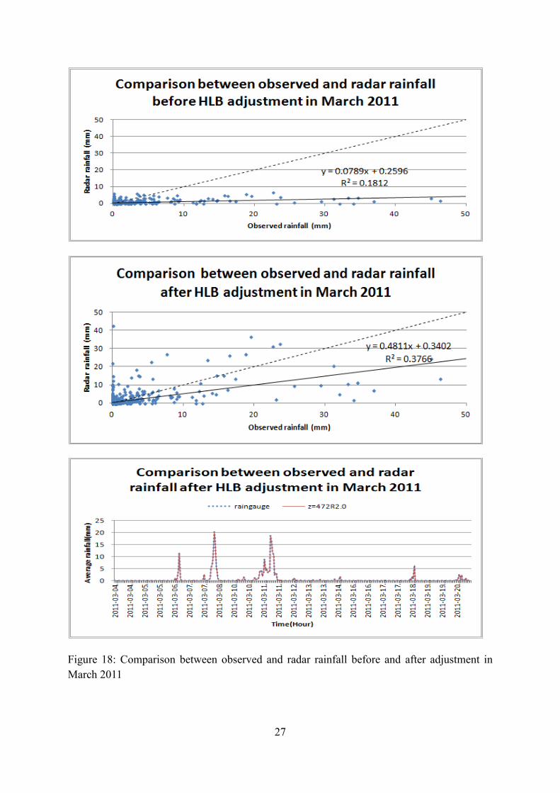
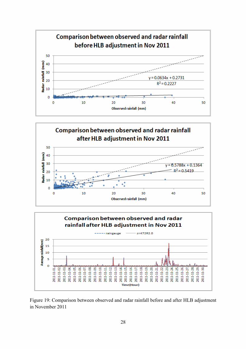
The results of new radar rainfall are displayed in Figure 18 and 19 for March 2011 and

November 2011 respectively with the time series analysis. Here, the hourly local bias is already

corrected but some rainfalls attain either underestimate or overestimate values. The

computation of RMSE and total error are more emphasized than the linear regression

coefficient (R2). Although HLB method can reduce the error estimation on RMSE compare to

MFB method, still the accurate radar rainfall estimation cannot be obtained. The adjusted radar

rainfalls need the ratio 4 to 5 to correct bias relatives to gauges. This value is also probably

influenced by the obstacles and shielding.

On the other hand, this is possibly happened because of the quality of radar data which the

radar reflectivity always receives by the stations nearest to the radar. Salek, et al.,(2004)

mentioned that averaging in radar reflectivity introduces a bias because reflectivity is

nonlinearly related to the rain intensities. This bias increases with the inhomogeneity of the

reflectivity field especially with the distance of radar. It will produce large errors in the bright

band which usually occur during stratiform or stable situation. Stratiform precipitation also

known as large-scale or synoptic-scale is caused by upward vertical motion over large areas

due to synoptic-scale forcing.

27

Figure 18: Comparison between observed and radar rainfall before and after adjustment in

March 2011

28

Figure 19: Comparison between observed and radar rainfall before and after HLB adjustment

in November 2011

29

From all those analysis on calibration and validation, the MFB and HLB adjustment have its

own advantages and disadvantages. MFB can adjust the parameter a in Z-R relationship which

can provide the same amount of total rainfall. However, when the analysis on the hourly time

series is done the radar rainfalls sometimes much more underestimate than the observed rainfall

due to the spatial variation since MFB is only emphasized on the constant time and space

(Hanchoowong, et.al., 2012). MFB method is suitable on the dense rain gauge network areas

and provides the persistence in Z-R relationship. After applying HLB correction method, the

error estimation can be reduced, nevertheless provide inaccuracy radar rainfall estimation. This

HLB method can be applied to areas where rain gauge networks are dense with long historical

rainfall records since it considers the same climatological rainfall characteristics in the rainfall

adjustment. However, it is emphasized that the reduction of bias in hourly period is vital for

hydrological application since the rainfall in hourly basis. In conclusion, the uncertainty still

remains in the estimated bias HLB ratios although these two kinds of bias adjustments are

applied.

4.2 RRI Model Output

Rainfall distribution is an important input in the RRI model. This study utilized the radar

rainfall estimation with bias correction HLB and MFB. A comparison between radar rainfall

and observed rainfall in November 2011 and March 2011 is made for the better analysis. The

purpose of applying the RRI model is to obtain the inundation area for the early warning

system. The locations of the predicted inundation area are very essential to deliver accurately

and timely warning. Firstly, the model parameters to apply in the simulation are determined by

considering the soil type or surface/subsurface flow conditions. The characteristics of the basin

should be known for a better understanding in selecting the parameters to run hydrological

model. Nonetheless, the width and depth of the cross sections do not know, hence these

parameters are employed by trial and error until the results of simulation discharge are similar

compared to the observed. Other boundary conditions such as levee height, the location of dams

or embankments should be identified before running this model.

In Kuantan river Basin, there is no influence by dam or reservoirs when executing this model.

The simulation is conducted for the period 01 March 2011 (0:00LT) to 20 March 2011(0:00LT)

in hourly basis. The hourly rainfall input from this data is calculated by Rain Thiessen Polygon

method by utilizing FORTRAN programming. The inundation area and peak discharge can be

observed after running the program RRI_input. The observed and simulated discharges are

compared to check the accuracy of the used parameters. After calibration, the validation of the

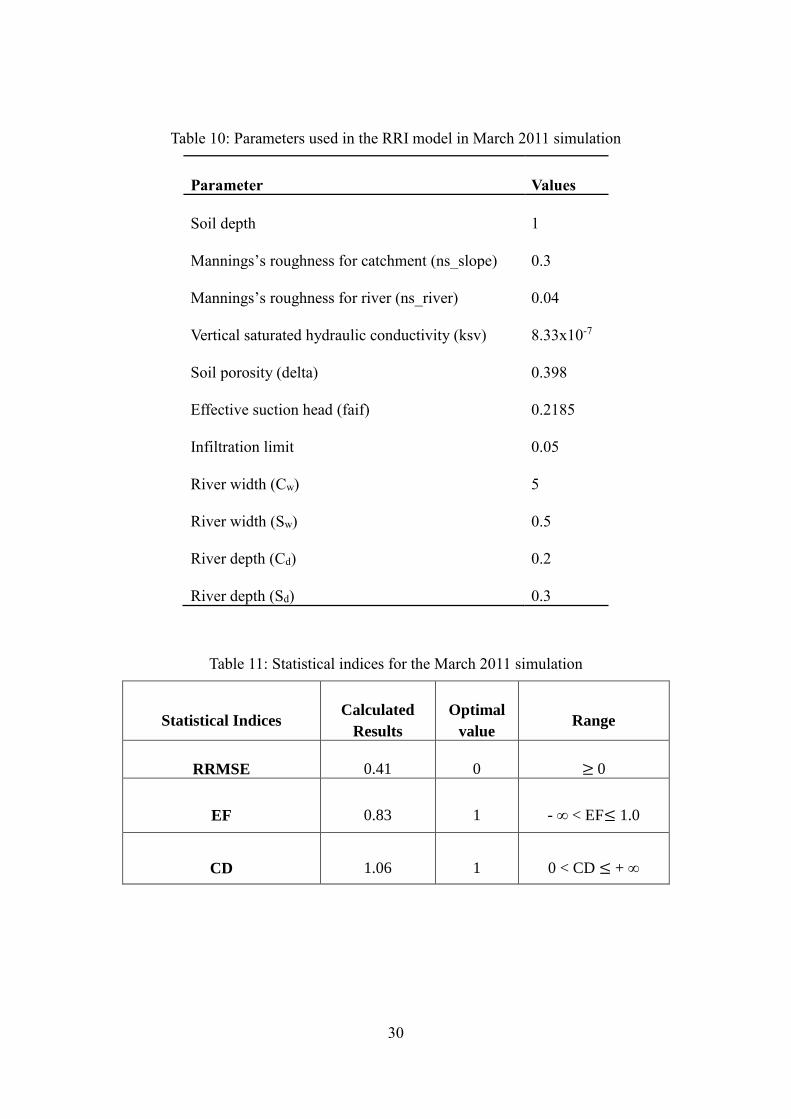
parameters for the rainfall data from 01-30 November 2011 is performed. Table 10 shows the

parameters used for this simulation. The statistical indices for the March 2011 simulation are

attached in Table 11.

30

Table 10: Parameters used in the RRI model in March 2011 simulation

Parameter Values

Soil depth 1

Mannings’s roughness for catchment (ns_slope) 0.3

Mannings’s roughness for river (ns_river) 0.04

Vertical saturated hydraulic conductivity (ksv) 8.33x10-7

Soil porosity (delta) 0.398

Effective suction head (faif) 0.2185

Infiltration limit 0.05

River width (Cw) 5

River width (Sw) 0.5

River depth (Cd) 0.2

River depth (Sd) 0.3

Table 11: Statistical indices for the March 2011 simulation

Statistical Indices Calculated

Results

Optimal

value Range

RRMSE 0.41 0 ≥ 0

EF 0.83 1 - ∞ < EF≤ 1.0

CD 1.06 1 0 < CD ≤ + ∞

31

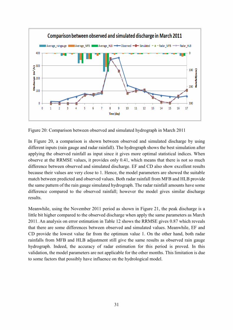
Figure 20: Comparison between observed and simulated hydrograph in March 2011

In Figure 20, a comparison is shown between observed and simulated discharge by using

different inputs (rain gauge and radar rainfall). The hydrograph shows the best simulation after

applying the observed rainfall as input since it gives more optimal statistical indices. When

observe at the RRMSE values, it provides only 0.41, which means that there is not so much

difference between observed and simulated discharge. EF and CD also show excellent results

because their values are very close to 1. Hence, the model parameters are showed the suitable

match between predicted and observed values. Both radar rainfall from MFB and HLB provide

the same pattern of the rain gauge simulated hydrograph. The radar rainfall amounts have some

difference compared to the observed rainfall; however the model gives similar discharge

results.

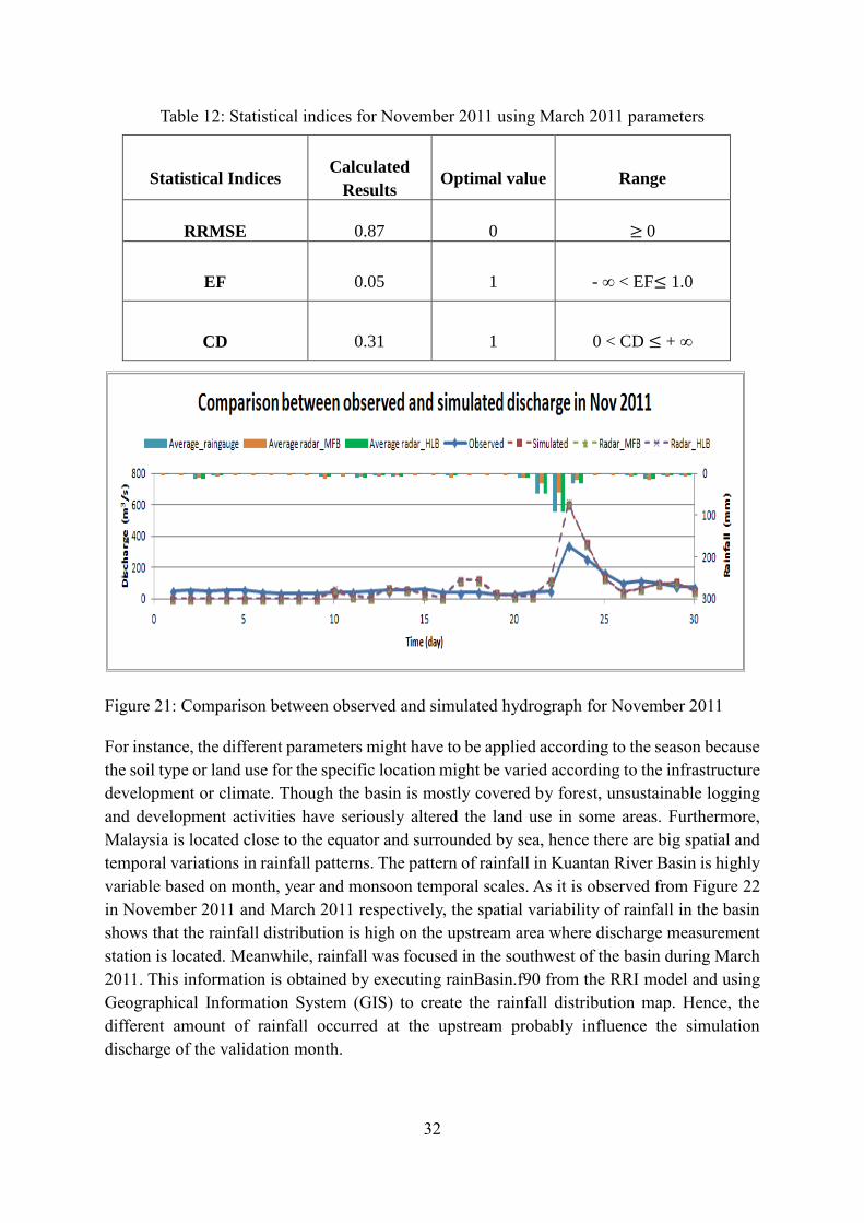
Meanwhile, using the November 2011 period as shown in Figure 21, the peak discharge is a

little bit higher compared to the observed discharge when apply the same parameters as March

2011. An analysis on error estimation in Table 12 shows the RRMSE gives 0.87 which reveals

that there are some differences between observed and simulated values. Meanwhile, EF and

CD provide the lowest value far from the optimum value 1. On the other hand, both radar

rainfalls from MFB and HLB adjustment still give the same results as observed rain gauge

hydrograph. Indeed, the accuracy of radar estimation for this period is proved. In this

validation, the model parameters are not applicable for the other months. This limitation is due

to some factors that possibly have influence on the hydrological model.

32

Table 12: Statistical indices for November 2011 using March 2011 parameters

Statistical Indices Calculated

Results Optimal value Range

RRMSE 0.87 0 ≥ 0

EF 0.05 1 - ∞ < EF≤ 1.0

CD 0.31 1 0 < CD ≤ + ∞

Figure 21: Comparison between observed and simulated hydrograph for November 2011

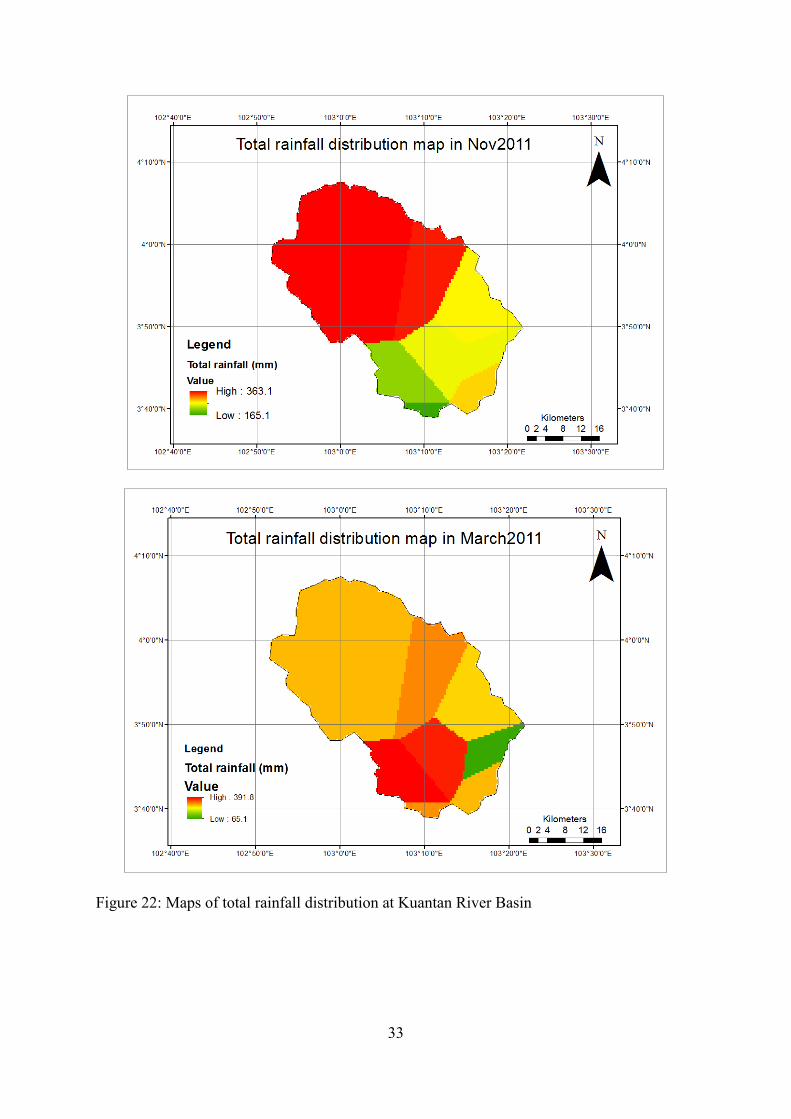
For instance, the different parameters might have to be applied according to the season because

the soil type or land use for the specific location might be varied according to the infrastructure

development or climate. Though the basin is mostly covered by forest, unsustainable logging

and development activities have seriously altered the land use in some areas. Furthermore,

Malaysia is located close to the equator and surrounded by sea, hence there are big spatial and

temporal variations in rainfall patterns. The pattern of rainfall in Kuantan River Basin is highly

variable based on month, year and monsoon temporal scales. As it is observed from Figure 22

in November 2011 and March 2011 respectively, the spatial variability of rainfall in the basin

shows that the rainfall distribution is high on the upstream area where discharge measurement

station is located. Meanwhile, rainfall was focused in the southwest of the basin during March

2011. This information is obtained by executing rainBasin.f90 from the RRI model and using

Geographical Information System (GIS) to create the rainfall distribution map. Hence, the

different amount of rainfall occurred at the upstream probably influence the simulation

discharge of the validation month.

33

Figure 22: Maps of total rainfall distribution at Kuantan River Basin

34

Since river discharge is affected by amount of water within a watershed, it increases with

rainfall and decreases during dry period. Hence, the infiltration limits have impact on this

pattern of the hydrograph. Infiltration can be defined as the entry of water into the soil surface

and its subsequent vertical motion through soil profile. Many factors influence the infiltration

rate including the condition of the soil surface and its vegetation cover, the properties of soil

and current moisture content of the soil. Depending on the amount of infiltration and the

physical properties of the soil, the river discharge may vary from time to time. The intensity of

infiltration value becomes lower when all of the precipitation seeps into the pores (Brutsaert,

2005). In the March 2011 simulation, a value of 0.05 for the infiltration limit was obtained by

calibration. This indicates that more water reaches the river than is lost due to the infiltration.

Nevertheless, the infiltration limit should be greater than 0.05 because February is the dry

period which is greatly influenced the soil moisture content.

Apart from that, more meteorological and hydrological stations are needed, especially in the

upstream areas, to identify the areas which contribute most to runoff and river discharge.

Consequently, the radar coverage is very significant to provide this kind of poor rain-gauge

river basin. For the further analysis, the development of the spatial distribution of radar rainfall

estimation in each grid point will be established to estimate the better watershed runoff and

inundation areas.

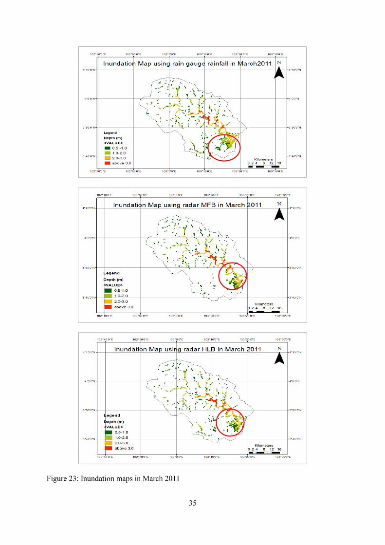
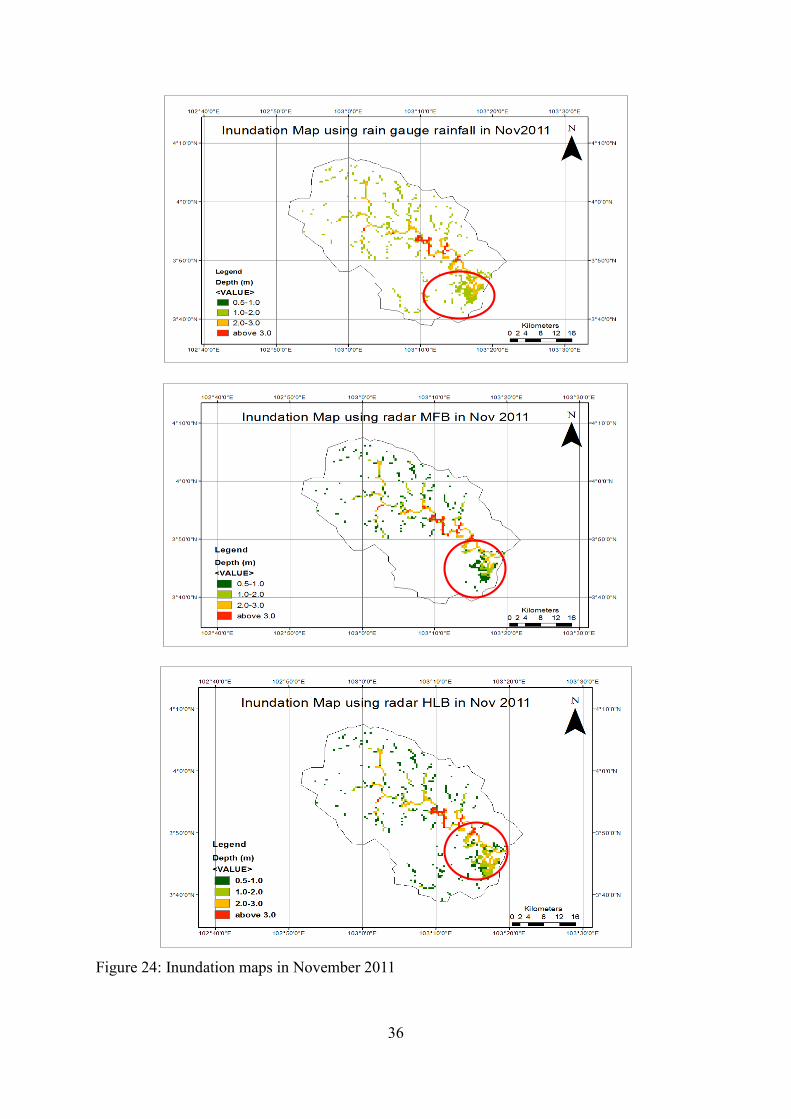
In addition, an assessment of the images of the inundation map based on the observed and radar

rainfall is studied. Figure 23 and 24 describe the inundation area at Kuantan River Basin in

March 2011 and November 2011 respectively. From these figures, the location of inundation

area can be identified which is necessary for the early warning system. Since all the warning

issuances are needed to state the locations probably inundated, this model can provide sufficient

information for emergency response. From these figures, the difference in inundation depth

occurred in this basin can be noticed. The red circle indicates the difference of inundation area

and depth by applying the different input of rainfall. In the inundation map simulated by using

MFB radar rainfall, the locations of inundation and flood depths are quite different compare to

the observed rainfall as an input. Meanwhile, by using HLB radar rainfall both on inundation

areas and depths look similar with that simulated by using the observed rainfall. Furthermore,

the inundation maps simulated by using MFB and HLB radar rainfall are differ from each other

in terms of location and depth especially in the red circle area. This is occurred due to the

different estimation of rainfall by using the adjustment methods which HLB can produce the

accurate estimation compare to the MFB method. It is proved that the radar rainfall estimation

in hourly basis should be accurate to provide the better estimation on inundation areas,

especially in the flood prone areas. In conclusion, the radar rainfall as input data can be applied

in simulating RRI model to identify the specific inundation areas for the better providence of

early warning systems.

35

Figure 23: Inundation maps in March 2011

36

Figure 24: Inundation maps in November 2011

37

5. CONCLUSIONS

The main objective of this study is to obtain the accurate radar rainfall estimation as input into

flood forecasting model. Hence, the investigation of radar information in Pahang is selected to

achieve this purpose. The separation of radar data according to the season is established to

compare with the Rosenfeld relationship which is commonly used for rainfall estimation in

Malaysia. The technique to derive the new relationship is also investigated and attained the

non-linear regression method would be the most excellent method. Furthermore, the radar

reflectivity data on the threshold 15 and 53 gain the finest result since it can reduce the error

from radar noise and hail contamination.

The radar rainfalls are extracted via the new derivation of Z-R relationship by employing mean

field bias (MFB) and modification of Z-R relationship simultaneously. Using these two kinds

of method for calibration, they show the best results only on the spatial distribution. This means

that they only focused on the total amount of rainfall. When the time series analysis is

investigated, the results seem inaccurate. Range dependent analysis has been done to know the

factor influence on the low quality of results using the all rain gauge stations before proceeding

to the further analysis. As a result, the radar reflectivity signal at the most location on the

western part is very low due to the mountainous area. Besides, the location of radar situated in

the nearby buildings and hills reduce the accuracy of radar rainfall estimation.

The analysis has been continued by excluding the stations in the shadow area. By applying

MFB and modification of Z-R relationship using non-linear regression method, the good Z-R

relationship according to the season can be found. In the northeast and the southwest monsoon,

Z=472R2.0 and Z=401R1.2 are applied for the rainfall estimation respectively. These

relationships can be employed in other months proved that they are successfully applied in the

each season. It is also evident that the convective and stratiform Z-R relationships are essential

for improving the performance of radar rainfall estimation when comparing to the rainfall

estimation by Rosenfeld relationship. The adjustment methods are needed because they are the

key factor in achieving high-quality radar estimates. Thus, firstly the adjustment of the rainfall

estimation by MFB method is selected. Although MFB method give the same amount of

rainfall, analysis on the time series does not show the best results since the hourly rainfall as

input data in hydrological model plays an important role on the flood forecasting. This is

because MFB method just emphasized on the constant temporal and spatial distribution only.

More dense of rain gauge networks are needed for the better quantitative rainfall estimation

when apply this method.

Therefore, hourly local bias correction (HLB) has been proposed because an adjustment in

hourly interval can provide best radar rainfall estimation. This method can reduce the RMSE

and adjust the total rainfall to be similar with the observed. But, these two methods need to

improve by considering long historical records and dense rain gauge networks. On the other

hand, the radar rainfall estimation still has its inadequacy because of the contamination of radar

data quality. Though the reflectivity within the threshold 15<dBZ<53 are included, the data

still effects by the ground clutter. The most significant factor that influence in this estimation

38

is the elevation angle of the antenna which the radar beam expansion is respected to the radar

range. Elevation angle 0.0 severely impacts the radar contamination because of the ground

clutter effects. Data quality is very essential in development of QPE by reducing the permanent

echoes to prevent uncertainty rainfall estimation. In conclusion, the objective to obtain the

accurate rainfall estimation should consider the errors effect to the radar as well as the rain

gauge.

After obtaining the radar rainfall, the RRI model is applied by using rainfall data because this

hydrological model can predict the inundation area. This is most vital to the issuance of early

warning system. The accuracy of radar rainfall is compared with the observed rainfall in term

of river discharge and inundation areas. Initially, the selected of model parameters are difficult

to determine for those who do not know well about hydrological characteristics for the basin.

Then, calibration and validation of the parameters have done for the other month and found

that there existed an error between the observed and simulated discharge for the validation. As

a result, the hydrological parameters are varied depending on the characteristics of the soil type

or seasons outlook.

The infiltration limit is the most important parameter that influences the conditions of river

discharge with considering the properties of soil and the current moisture content of soil.

Infiltration limit 0.05 gives the higher river discharge in November 2011 because in this month,

the saturated land cause of the most water precipitation goes to the river. Although March 2011

parameter is suitable to use itself, model parameters for other months should be evaluated since

the fluctuation of soil properties and land use because of the climate and infrastructure

developments. Apart from that, the inundation area information is varied according to the

adjustment method of radar rainfall estimation. MFB revealed the less accurate of inundation

area compare with HLB method which better in the estimation as well as the inundation depth.

However, after making the improvement of radar rainfall estimation by applying the adjustment

in more rain gauge networks and good quality of radar, the results are expected to be more

accurate. In conclusion, the radar rainfall as input data is proved can be applied in simulating

RRI model to identify the inundation area and depth for the better providence of early warning

systems.

39

REFERENCES

A.Smith, J., and F.Krajewski, W. (1991). Estimation of the mean field bias of radar rainfall

estimates. Journal of Applied Meteorology , Volume 30, No.4 , pp. 397-412.

Abu Samah, A., and Lim, J. T. (2004). Weather and Climate of Malaysia. University of Malaya

Press.

Agency, J. M. (2000). Algorithms for precipitation nowcasting focused on detailed analysis

using radar and raingauge data. Japan Meteorology Agency, No.39, pp. 63-111.

Amin, M.S.M., Waleed, A.R.M., and Aimrun, W. (2010). Improving Efffective Rainfall Using

Virtual Stations With Radar-Derived Data. The 61st International Executive Council Meeting

and the 6th Asian Regional Conference, Yogyakarta, Indonesia. pp. 1-8.

Brutsaert, W. (2005). Hydrology An Introduction. Cambridge: Cambridge University Press.

Chumchean, S., Sharma, A., and Seed, A. (2006). An Integrated Approach to Error Correction

for Real-Time Radar Rainfall Estimation. Volume 23, pp. 67-79

Clarke, B., Kudym, C., and Rindahl, B. (2009). Gauge-Adjusted Radar Rainfall Estimation

and Basin Averaged Rainfall for use in Local Flash Flood Prediction and Runoff Modeling.

23rd Conference on Hydrology, Phoenix, AZ.

Collinge, V., and Kirby, C. (1987). Weather Radar and Flood Forecasting. John Wiley & Sons

Ltd.

da Silva Moraes, M. C., Sarmento Tenorio, R., and Baldicero Molion, L. C. (2006). Z-R

Relationship for a weather radar in the eastern coast of northeastern Brazil. International

Journal of Maritime and Communication Science, Volume 4, No. 4, pp.41-45

Division, H. a. (2012). Flood Report at Kuantan, Pahang on the 24th Dec 2012. Department

of Irrigation and Drainage.

E.Gregow, E.Saltikoff, S. Albers, and H. Hohti., (2013). Precipitation accumulation analysis-

assimilation of radar-gauge measurements and validation of different methods. Hydrology

and Earth System Sciences , No.10, pp.2453-2480.

E.Rinehart, R. (2004). Radar for Meteorologists (Fourth ed.). Columbia: Rinehart Publications.

Haji Khamis, N. H., Din, J., and Abdul Rahman, T. (2005). Rainfall Rate from Meteorological

Radar Data for Microwave Applications in Malaysia. IEEE. pp.1008-1010.

40

Hanchoowong, R., Weesakul, U., and Chumchean, S. (2012). Bias correction of radar rainfall

estimates based on geostatical technique. ScienceAsia 38, pp.373-385.

He, X., Vejen, F., Stisen, S., O.Sonnenborg, T., and H.Jensen, K. (2011). An Operational

Weather Radar-Based Quantitative Precipitation Estimation and Its Application in

Catchment Water Resources Modelling. Volume 10, pp.8-24

Holleman, I. (2006). Bias Adjustment of radar-based 3-hour precipitation accumulations.

Technical Report, KNMI TR-290, pp.1-56

J.Doviak, R., and S.Zrnic, D. (1993). Doppler Radar and Weather Observations. (Second Ed.),

Academic Press.

K.C.Low. (2006). Application of Nowcasting Techniques Towards Strengthening National

Warning Capabilities on Hydrometeorological and Landslides Hazards. Sydney: Public

Weather Services Workshop on Warning of Real-Time Hazards by Using Nowcasting

Technology.

L.Alfieri, P.Claps, and F.Laio. (2010). Time-dependant Z-R relationship for estimating rainfall

fields from radar measurements. Natural Hazard and Earth System Sciences , 10, pp.149-

158.

L.S. Kumar., Y.H. Lee, J.X. Yeo, and J.T. Ong. (2011). Tropical rain classification and

estimation of rain from Z-R(Reflectivity-Rain Rate) relationships. Progress in

electromagnetics Research B, Volume 32, pp.107-127.

Legrand, S., Dommanget, E., Graff, B., and Bontron, G. (2012). Use of radar QPE as an iput

to rainfall-runoff model:the case of the rhone River (France). The Seventh European

Conference on Radar in Meteorology and Hydrology, ERAD 2012, France.

Mat Adam, M. K., and Moten, S. (2012). Rainfall Estimation from Radar Data. Malaysian

Meteorological Department. Research Publication No.6/2012. pp.1-16.

Matsuura, T., Fukami, K., and Yoshitani, J. (2003). Evaluation of the applicability of radar

rainfall information to operational hydrology. Weather Radar Information and Distributed

Hydrological Modelling, IAHS Publ.No. 282, pp.24-29.

Mohd Nasir, M. F., Abdul Zali, M., Juahir, H., Hussain, H., M Zain, S., and Ramli, N. (2012).

Application of receptor models on water quality data in source apportionment in Kuantan

River Basin. Iranian Journal of Environmental Health Science and Engineering, 9:18, pp.1-

12

41

Morin, E., and Gabella, M. (2007). Radar-based quantitative precipitation estimation over

Mediterranean and dry climate regimes. Journal of Geophysical Research , Volume 112,

pp.1-13.

R, Suzana., and T, Wardah. (2011). Radar Hydrology : New Z/R Relationships for Klang River

Basin. 2011 International Conference on Environment Science and Engineering , Volume

8(2011), pp.248-251.

R. Suzana, T. Wardah, and A.B. Sahol Hamid. (2011). Radar Hydrology : New Z/R

Relationships for Klang River Basin Malaysia based on rainfall Classification. World

Academy of Science, Engineering and Technology 59 , pp.1994-1998.

Salek, M., Cheze, J.-L., Handwerker, J., Delobbe, L., and Uijlenhoet, R. (2004). Radar

techniques for identifying precipitation type and estimating quantity of precipitation.

Document of COST Action 717,WG 1. pp.1-51.

Sayama, T. (2013). Rainfall-Runoff-Inundation (RRI) Model. International Centre for Water

Hazard and Risk Management (ICHARM), Public Works Research Institute (PWRI).

Version 1.3.

Sayama, T., Ozawa, G., Kawakami, T., Nabesaka, S., and Fukami, K. (2012). Rainfall-runoff-

inundation analysis of the 2010 Pakistan flood in the Kabul River Basin. Hydrological

Sciences Journal, 57(2), pp.298-312.

Sebastianelli, S., Russo, F., Napolotano, F., and Baldini, L. (2010). Comparison between radar

and raingauges data at different distances from radar and correlationexisting between the

rainfall values in the adjacent pixels. Taormina, Italy: International Workshop Advances in

Statistical Hydrology. pp.1-10.

Shafie, A. (2009). Extreme Flood Event : A case study on Floods of 2006 and 2007 in Johor,

Malaysia. Technical Report, Colorado State University, pp.2.

Tadesse, A., and N.Anagnostou, E. (2005). A statistical approach to ground radar-rainfall

estimation. Journal of Atmospheric and Oceanic Technology , Volume 22, pp.1720-1731.

Tekolla, W. A. (2010). Rainfall and Flood Frequency Analysis for Pahang River Basin,

Malaysia. Lund University, Sweden. pp.2-7.

Uijlenhoet, R. (2001). Raindrop size distribution and radar reflectivity-rain rate relationships

for radar hydrology. Hydrology and Earth System Sciences, 5(4), pp.615-627.

V.Lopez, F.Napolitano, and F.Russo. (2005). Calibration of a rainfall-runoff model using radar

and raingauge data. Advances in Geosciences, 2, pp.41-46.

42

Ven, T. C., Maidment, D. R., and Mays, L. W. (1988). Applied Hydrology. McGraw-Hill Book

Company.

Website: Climate of Malaysia, Malaysian Meteorological Department (MMD),

http://www.met.gov.my

Website: Conventional radar lecture notes

http://apollo.lsc.vsc.edu/classes/remote/lecture_notes/radar/conventional.html

Website: Flood Management, Department of Irrigation and Drainage (DID)

http://www.water.gov.my

Website: IRIS Vaisala Sigmet, VAISALA

http://www.vaisala.com/en/hydrology/offering/weatherradars/Pages/IRIS.aspx

Website: Map of Malaysia https://www.cia.gov/library/publications/the-world-

factbook/geos/my.html

Website : M.Hunter, S. (1996). WSR-88D Radar Rainfall Estimation: Capabilities, Limitations

and Potential Improvements. National Weather Service (NOAA)

http://www.srh.noaa.gov/mrx/research/precip/precip.php

Yokoi, S., Nakayama, Y., Agata, Y., Satomura, T., Kuraji, K., and Matsumoto, J. (2012). The

relationship between observation intervals and errors in radar rainfall estimation over the

Indochina Peninsula. Hydrological Process, Volume 26, Issue 6, pp.834-842.

43

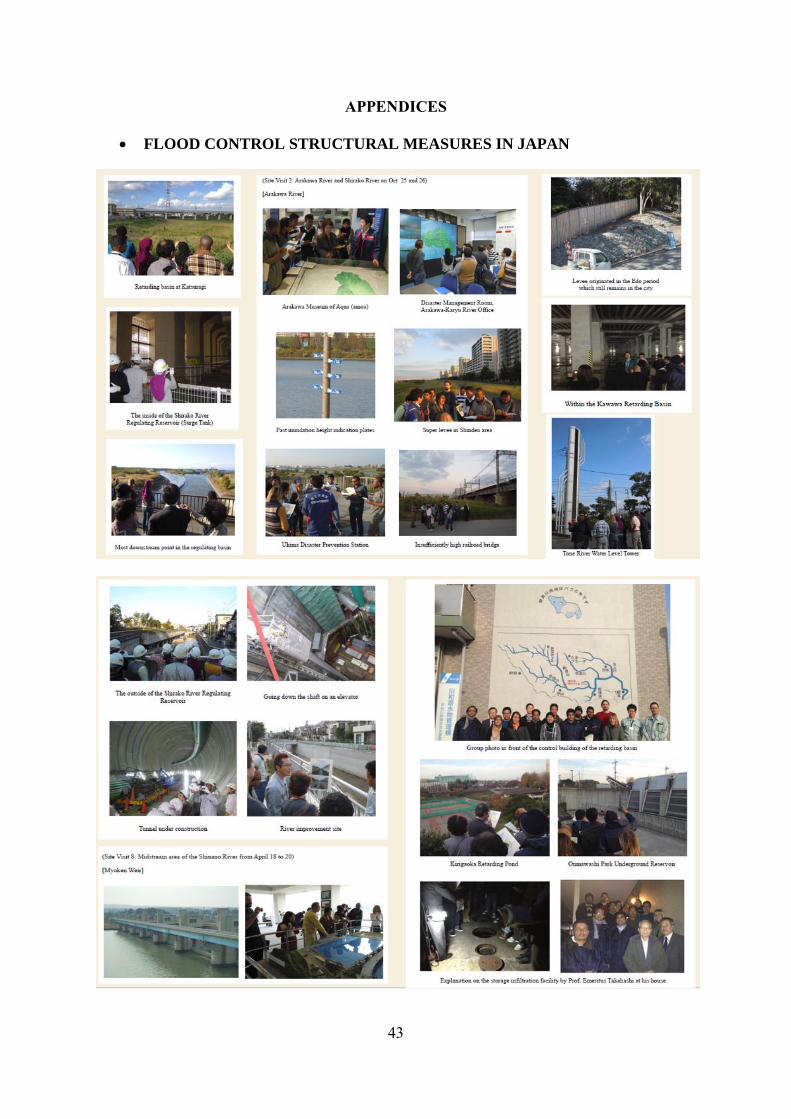
APPENDICES

FLOOD CONTROL STRUCTURAL MEASURES IN JAPAN

44

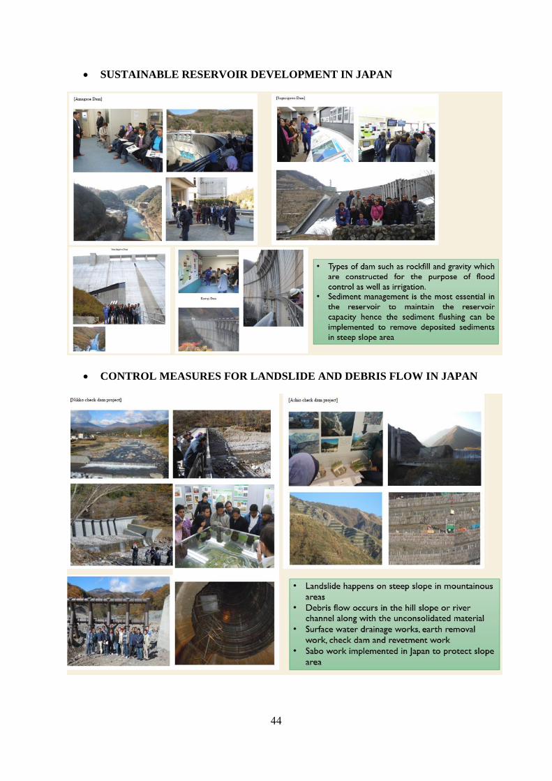
SUSTAINABLE RESERVOIR DEVELOPMENT IN JAPAN

CONTROL MEASURES FOR LANDSLIDE AND DEBRIS FLOW IN JAPAN

45

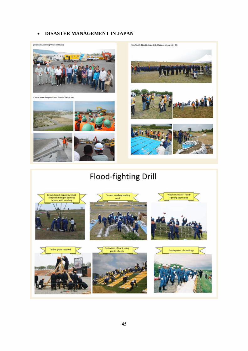
DISASTER MANAGEMENT IN JAPAN