Research Paper Simulation of Double Pendulum · Simulation of Double Pendulum Abdalftah Elbori1, Ltfei Abdalsmd2 1(MODES Department, Atılım University Turkey)

Quest Journals

Journal of Software Engineering and Simulation

Volume 3 ~ Issue 7 (2017) pp: 01-13

ISSN(Online) :2321-3795 ISSN (Print):2321-3809

www.questjournals.org

*Corresponding Author: Abdalftah Elbori 1 | Page

MODES Department Atilim University Turkey

Research Paper

Simulation of Double Pendulum

Abdalftah Elbori1, Ltfei Abdalsmd

2

1(MODES Department, Atılım University Turkey)

2(Material Science Department, Kastamonu University Turkey)

Received 01 Apr, 2017; Accepted 12 Apr, 2017 © The author(s) 2017. Published with open access at

www.questjournals.org

ABSTRACT : In this paper, the simulation of a double pendulum with numerical solutions are discussed. The

double pendulums are arranged in such a way that in the static equilibrium, one of the pendulum takes the

vertical position, while the second pendulum is in a horizontal position and rests on the pad. Characteristic

positions and angular velocities of both pendulums, as well as their energies at each instant of time are

presented. Obtained results proved to be in accordance with the motion of the real physical system. The

differentiation of the double pendulum result in four first order equations mapping the movement of the system.

Keywords: Double Pendulum, Numerical Solution, Simulation, Behaviors of the System

I. INTRODUCTION A pendulum is a weight suspended from a pivot so that it can swing freely. When a pendulum is

displaced sideways from its resting equilibrium position, it is subject to a restoring force due to gravity that will

accelerate it back toward the equilibrium position [1] and [2] . When released, the restoring force combined with

the pendulum's mass causes it to oscillate about the equilibrium position, swinging back and forth. The time for

one complete cycle, a left swing and a right swing, is called the period. The period depends on the length of the

pendulum and also on the amplitude of the oscillation. However, if the amplitude is small, the period is almost

independent of the amplitude [3] and [4].

Double pendulum is a mechanical system that is most widely used for demonstration of the chaotic

motion. It is described with two highly coupled, nonlinear, 2nd order ODE’s which makes is very sensitive to

the initial conditions[5] and [6]. Although its motion is deterministic in nature, sensitivity to initial conditions

makes its motion unpredictable or ‘chaotic’ in the long turn in this paper discusses in the first part purpose of the

double pendulum [7], in the second section, the system of coordinates is presented and in the third section, the

equations of motion it’s numerical solutions are investigated by using ODEs 45. Whereas in the final section,

behavior of the system and simulation of the double pendulum are discussed by this paper and explain how to

linearize the double pendulum investigate modeling the Linearization Error.

This paper is not only analyzed the dynamics of the double pendulum system and discussing the

physical system, but also explain how the Lagrange and the Hamiltonian equations of motions are derived, we

will analyze and compare between the numerical solution and simulation, and also change of angular velocities

with time for certain system parameters at varying initial conditions.

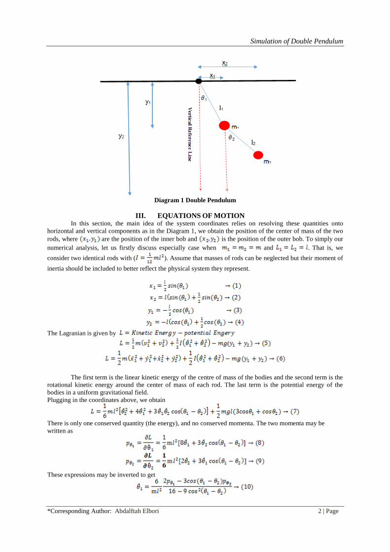
II. SYSTEM COORDINATES The double pendulum is illustrated in Diagram1. It is convenient to define the coordinates in terms of

the angles between each rod and the vertical. In this Diagram 1 , and represent the mass, length and the

angle from the normal of the inner bob and , and stand for the mass, length, and the angle from the

normal of the outer bob. The simple kinematics equations represent in next section to derive equations of motion

by using Lagrange equations

http://www.questjournals.org/



Diagram 1 Double Pendulum

III. EQUATIONS OF MOTION In this section, the main idea of the system coordinates relies on resolving these quantities onto

horizontal and vertical components as in the Diagram 1, we obtain the position of the center of mass of the two

rods, where are the position of the inner bob and is the position of the outer bob. To simply our

numerical analysis, let us firstly discuss especially case when and . That is, we

consider two identical rods with ( ). Assume that masses of rods can be neglected but their moment of

inertia should be included to better reflect the physical system they represent.

The Lagranian is given by

(

The first term is the linear kinetic energy of the centre of mass of the bodies and the second term is the

rotational kinetic energy around the center of mass of each rod. The last term is the potential energy of the

bodies in a uniform gravitational field.

Plugging in the coordinates above, we obtain

There is only one conserved quantity (the energy), and no conserved momenta. The two momenta may be

written as

These expressions may be inverted to get



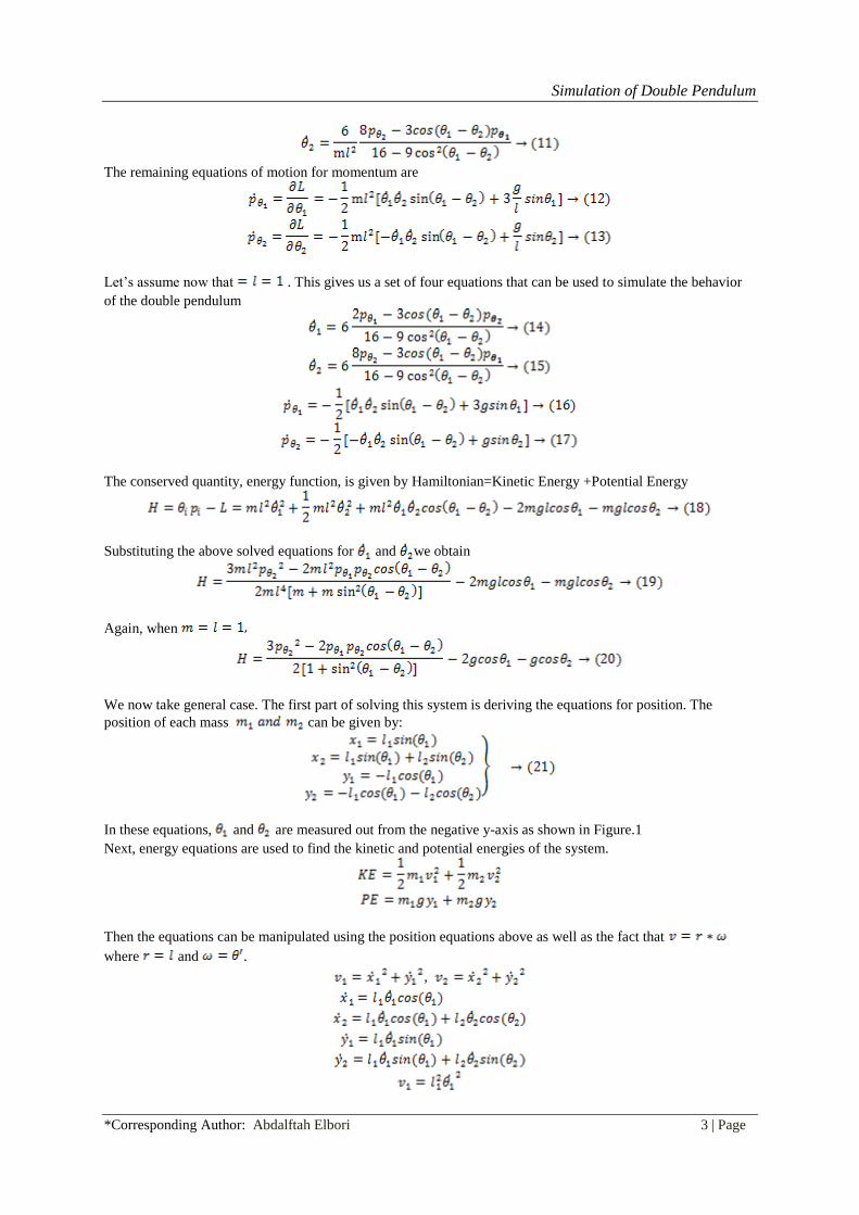
The remaining equations of motion for momentum are

Let’s assume now that . This gives us a set of four equations that can be used to simulate the behavior

of the double pendulum

The conserved quantity, energy function, is given by Hamiltonian=Kinetic Energy +Potential Energy

Substituting the above solved equations for and we obtain

Again, when

We now take general case. The first part of solving this system is deriving the equations for position. The

position of each mass can be given by:

In these equations, and are measured out from the negative y-axis as shown in Figure.1

Next, energy equations are used to find the kinetic and potential energies of the system.

Then the equations can be manipulated using the position equations above as well as the fact that

where and .

,



The Lagrange is the difference between the kinetic and potential equations of the system. It is used when a

system is stated as a set of generalized coordinates rather than velocities. In this case, the coordinates of the

system are based on and :

The second part of the Lagrange equation involves taking the partial of the above Lagrange equation with

respect to the generalized coordinates. This will give two new equations

From Equation 23:

Then placing equation 25 into equation 24, equation 26 is developed:

The same thing is done with using equation 24:

Then placing this into equation 24:

Equation 26 and equation 28 are used to describe the motion of the pendulum’s system and are 2nd

-

order differential equations. This cannot yet be used in MATLAB because there are four unknowns. The system

motion must be described in first-order differential equations before ODE45 can be used. Momenta Equations.

The momenta, and , are found by taking the partial of the Lagrange with respect to and , respectively.

The momenta equations are described as the partial derivative of the Lagrange with respect to the angular

velocities. Therefore:

The Hamiltonian equation is for .The Hamiltonian will be used to put the equations in

terms of four initial conditions:

The momenta equations in equation 29 are then solved for and .These two equations are then placed into

equation 30 and the following equation is derived.



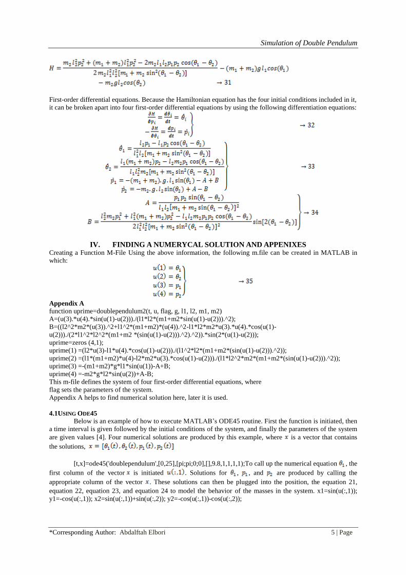
First-order differential equations. Because the Hamiltonian equation has the four initial conditions included in it,

it can be broken apart into four first-order differential equations by using the following differentiation equations:

IV. FINDING A NUMERYCAL SOLUTION AND APPENIXES Creating a Function M-File Using the above information, the following m.file can be created in MATLAB in

which:

Appendix A

function uprime=doublependulum2(t, u, flag, g, l1, l2, m1, m2)

A=(u(3).*u(4).*sin(u(1)-u(2)))./(l1*l2*(m1+m2*sin(u(1)-u(2))).^2);

B=((l2^2*m2*(u(3)).^2+l1^2*(m1+m2)*(u(4)).^2-l1*l2*m2*u(3).*u(4).*cos(u(1)-

u(2)))./(2*l1^2*l2^2*(m1+m2 *(sin(u(1)-u(2))).^2).^2)).*sin(2*(u(1)-u(2)));

uprime=zeros (4,1);

uprime(1) =(l2*u(3)-l1*u(4).*cos(u(1)-u(2)))./(l1^2*l2*(m1+m2*(sin(u(1)-u(2))).^2));

uprime(2) =(l1*(m1+m2)*u(4)-l2*m2*u(3).*cos(u(1)-u(2)))./(l1*l2^2*m2*(m1+m2*(sin(u(1)-u(2))).^2));

uprime(3) =-(m1+m2)*g*l1*sin(u(1))-A+B;

uprime(4) =-m2*g*l2*sin(u(2))+A-B;

This m-file defines the system of four first-order differential equations, where

flag sets the parameters of the system.

Appendix A helps to find numerical solution here, later it is used.

4.1USING ODE45

Below is an example of how to execute MATLAB’s ODE45 routine. First the function is initiated, then

a time interval is given followed by the initial conditions of the system, and finally the parameters of the system

are given values [4]. Four numerical solutions are produced by this example, where is a vector that contains

the solutions,

[t,x]=ode45('doublependulum',[0,25],[pi;pi;0;0],[],9.8,1,1,1,1);To call up the numerical equation , the

first column of the vector is initiated . Solutions for , , and are produced by calling the

appropriate column of the vector . These solutions can then be plugged into the position, the equation 21,

equation 22, equation 23, and equation 24 to model the behavior of the masses in the system. x1=sin(u(:,1));

y1=-cos(u(:,1)); x2=sin(u(:,1))+sin(u(:,2)); y2=-cos(u(:,1))-cos(u(:,2));



4.2 Behaviors of the System Depending on the given initial conditions, the double pendulum exhibits three types of behavior: •

Quasiperiodic motion • Periodic motion • Chaotic motion In this section, only Quasiperiodic motion is discussed

and explained in brief way.

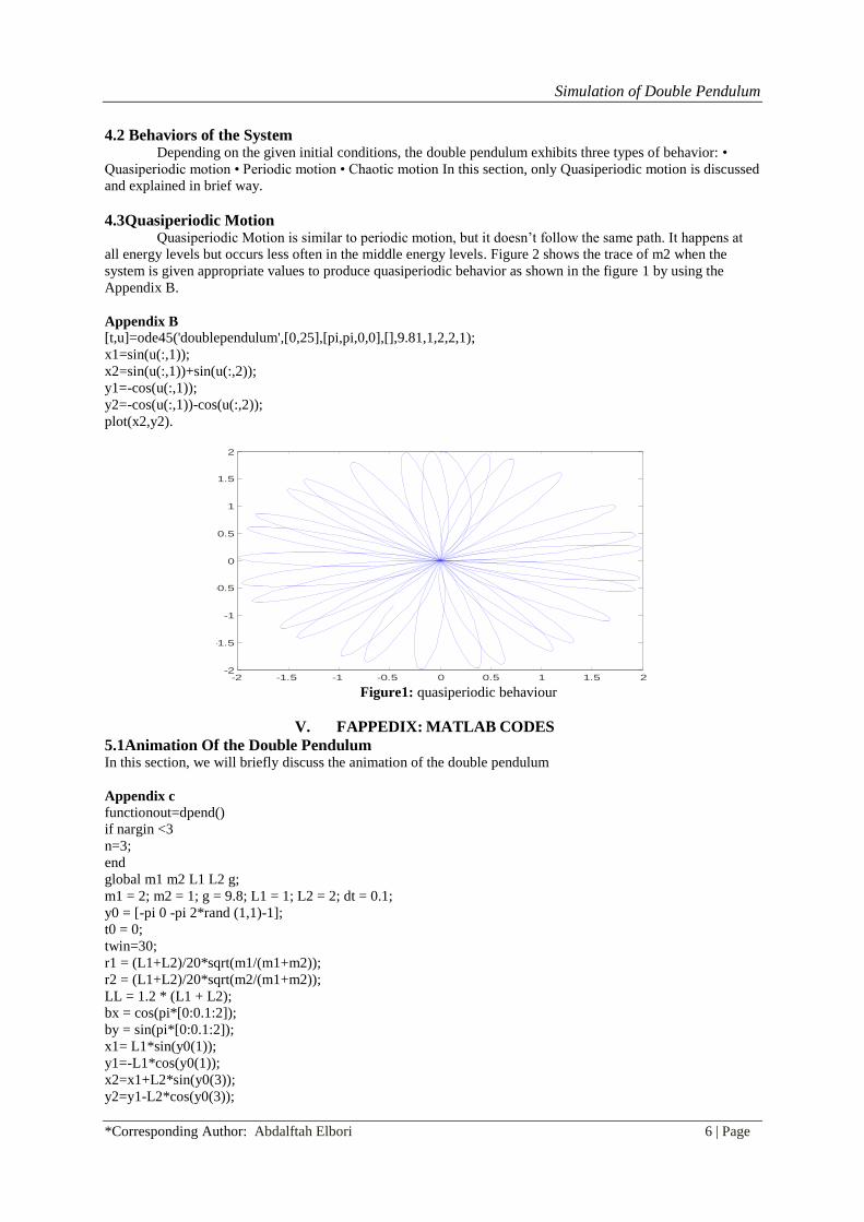
4.3Quasiperiodic Motion Quasiperiodic Motion is similar to periodic motion, but it doesn’t follow the same path. It happens at

all energy levels but occurs less often in the middle energy levels. Figure 2 shows the trace of m2 when the

system is given appropriate values to produce quasiperiodic behavior as shown in the figure 1 by using the

Appendix B.

Appendix B

[t,u]=ode45('doublependulum',[0,25],[pi,pi,0,0],[],9.81,1,2,2,1);

x1=sin(u(:,1));

x2=sin(u(:,1))+sin(u(:,2));

y1=-cos(u(:,1));

y2=-cos(u(:,1))-cos(u(:,2));

plot(x2,y2).

-2 -1.5 -1 -0.5 0 0.5 1 1.5 2-2

-1.5

-1

-0.5

0

0.5

1

1.5

2

Figure1: quasiperiodic behaviour

V. FAPPEDIX: MATLAB CODES

5.1Animation Of the Double Pendulum In this section, we will briefly discuss the animation of the double pendulum

Appendix c

functionout=dpend()

if nargin <3

n=3;

end

global m1 m2 L1 L2 g;

m1 = 2; m2 = 1; g = 9.8; L1 = 1; L2 = 2; dt = 0.1;

y0 = [-pi 0 -pi 2*rand (1,1)-1];

t0 = 0;

twin=30;

r1 = (L1+L2)/20*sqrt(m1/(m1+m2));

r2 = (L1+L2)/20*sqrt(m2/(m1+m2));

LL = 1.2 * (L1 + L2);

bx = cos(pi*[0:0.1:2]);

by = sin(pi*[0:0.1:2]);

x1= L1*sin(y0(1));

y1=-L1*cos(y0(1));

x2=x1+L2*sin(y0(3));

y2=y1-L2*cos(y0(3));



b4=plot([0,x1],[0,y1],'k-','LineWidth',2);

hold on

b3=plot([x1,x2],[y1,y2],'k-','LineWidth',2);

b1=fill(x1+r1*bx,y1+r1*by,'magenta');

b2=fill(x2+r2*bx,y2+r2*by,'black');

axis([-LL LL -LL LL])

for N=[1:1000]

posold=[x1 y1 x2 y2]';

yold=y0;

[t,y]=ode45('doublependulum2',[t0,t0+dt],y0,[],9.8,1,1,1,1);

y0=y(size(y,1),:);

clear y

clear t

y0(1)=mod(y0(1)+pi,2*pi)-pi;

y0(3)=mod(y0(3)+pi,2*pi)-pi;

t0=t0+dt;

x1 = L1*sin(y0(1));

y1 = - L1*cos(y0(1));

x2 = x1 + L2*sin(y0(3));

y2 = y1 - L2*cos(y0(3));

plot([posold(1) x1],[posold(2) y1],'magenta');

plot([posold(3) x2],[posold(4) y2],'black');

set(b4,'xdata',[0,x1],'ydata',[0,y1]);

set(b3,'xdata',[x1,x2],'ydata',[y1,y2]);

set(b1,'xdata',x1+r1*bx,'ydata',y1+r1*by);

set(b2,'xdata',x2+r2*bx,'ydata',y2+r2*by);

drawnow

pause(0.01)

end

figure(myfig);

pause

close(myfig)

-3 -2 -1 0 1 2 3

-3

-2

-1

0

1

2

3

Figure 2: Chaotic behaviour

5.2System of equations

Define a function that calculates the dynamics of the double pendulum flag determines initial positions

and velocities of the inner and outer bob. Equations 14 to 17 we save our file as Doublependulum2.m, and we

build it as

Appendix D

function xprime=doublependulum2(t, x, flag, g, l1, l2, m1, m2)

xprime=zeros (4,1);



xprime(1) = 6*(2*x(3)-3*cos(x(1)-x(2))*x(4))/(16-9*cos(x(1)-x(2))^2);

xprime(2) = 6*(8*x(4)-3*cos(x(1)-x(2))*x(3))/(16-9*cos(x(1)-x(2))^2);

xprime(3) = -(xprime(1)*xprime(2)*sin(x(1)-x(2))+3*g*sin(x(1)))/2;

xprime(4) = -(-xprime(1)*xprime(2)*sin(x(1)-x(2))+g*sin(x(2)))/2;

end

Now, our aim is calculating Energy of this function, which means we will use the equation 20 of Hamiltonian,

we save it as Hamiltonian.m,

function energy = hamiltonian(y0)

t1 = y0(1); t2 = y0(2); v1 = y0(3); v2 = y0(4); g = 9.8;

energy = abs(((3*(v2^2)-2*v1*v2*cos(t1-t2))/(2+2*(sin(t1-t2) ^2)))-2*g*cos(t1)-

g*cos(t2));

end

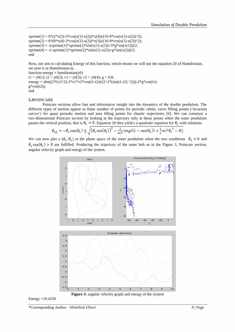
5.3POINCARE

Poincare sections allow fast and informative insight into the dynamics of the double pendulum. The

different types of motion appear as finite number of points for periodic orbits, curve filling points (‘invariant

curves’) for quasi periodic motion and area filling points for chaotic trajectories [6]. We can construct a

two‐dimensional Poincare section by looking at the trajectory only at those points when the outer pendulum

passes the vertical position, that is . Equation 20 then yield s a quadratic equation for with solutions

We can now plot a ( in the phase space of the inner pendulum when the two conditions and

are fulfilled. Producing the trajectory of the outer bob as in the Figure 3, Poincare section,

angular velocity graph and energy of the system.

-2 -1.5 -1 -0.5 0 0.5 1 1.5 2 2.5

-1.5

-1

-0.5

0

0.5

1

1.5

position

velo

city

trajectory

-500 -400 -300 -200 -100 0

-50

-40

-30

-20

-10

0

x1

x3

Poincare section (sin(x2)=0, increasing)

0 1 2 3 4 5 6 7 8 9 10-1.5

-1

-0.5

0

0.5

1

1.5

2

2.5

3

3.5Angular velocities

Figure 3: angular velocity graph and energy of the system

Energy =10.4250



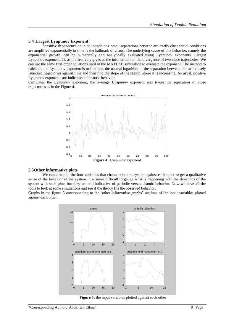
5.4 Largest Lyapunov Exponent Sensitive dependence on initial conditions small separations between arbitrarily close initial conditions

are amplified exponentially in time is the hallmark of chaos. The underlying cause of this behavior, namely the

exponential growth, can be numerically and analytically evaluated using Lyapunov exponents. Largest

Lyapunov exponents11, as it effectively gives us the information on the divergence of two close trajectories. We

can use the same first order equations used in the MATLAB simulation to evaluate the exponent. The method to

calculate the Lyapunov exponent is to first plot the natural logarithm of the separation between the two closely

launched trajectories against time and then find the slope of the region where it is increasing. As usual, positive

Lyapunov exponents are indicative of chaotic behavior.

Calculates the Lyapunov exponent, the average Lyapunov exponent and traces the separation of close

trajectories as in the Figure 4.

0 10 20 30 40 50 60 70 80 90 1000.4

0.6

0.8

1

1.2

1.4

1.6

1.8

2

average lyapunov exponent

Figure 4: Lyapunov exponent

5.5Other informative plots We can also plot the four variables that characterize the system against each other to get a qualitative

sense of the behavior of the system. It is more difficult to gauge what is happening with the dynamics of the

system with such plots but they are still indicative of periodic versus chaotic behavior. Now we have all the

tools to look at some simulations and see if the theory fits the observed behavior.

Graphs in the figure 5 corresponding to the ‘other informative graphs’ sections of the input variables plotted

against each other.

0 1 2 3 4-2

-1

0

1

2angular velocities

0 5 10 15 200

5

10

15angles

0 5 10 15 200

1

2

3

4positions and momentum of 1

0 5 10 15-2

-1

0

1

2positions and momentum of 2

Figure 5: the input variables plotted against each other



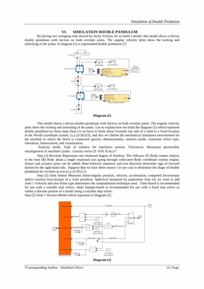
VI. SIMULATION DOUBLE PANDULUM By having two swinging rods slowed by sticky friction, let us build a model, this model shows a driven

double pendulum with stiction on both revolute joints. The angular velocity plots show the locking and

unlocking of the joints. In diagram (1) is represented double pendulum [7]

Scope2

Scope1

BF

Revolute1

BF

Revolute Joint1

Pulse

Generator

Env

Joint Sensor1

Joint Sensor

Joint 2 Velocity

Rev erse limit

Forward limit

Frictional torqueSensor

Actuator

Joint 2 Stiction Model

Joint 1 Velocity

TorqueRev erse limit

Forward limit

Frictional torqueSensor

Actuator

Joint 1 Stiction Model

Ground

CS

1

Body1

CS

1C

S2

Body

Diagram (2)

This model shows a driven double pendulum with stiction on both revolute joints. The angular velocity

plots show the locking and unlocking of the joints. Let us explain how we build the diagram (1) which represent

double pendulum by these steps Step (1) we have to think about Grounds one side of a Joint to a fixed location

in the World coordinate system. [x,y,z]=[0,0,0], and also we Define the mechanical simulation environment for

the machine to which the block is connected: gravity, dimensionality, analysis mode, constraint solver type,

tolerances, linearization, and visualization.

Analysis mode: Type of solution for machine's motion. Tolerances: Maximum permissible

misalignment of machine's joints. Gravity vector [0 -9.81 0]

Step (2) Revolute Represents one rotational degree of freedom. The follower (F) Body rotates relative

to the base (B) Body about a single rotational axis going through collocated Body coordinate system origins.

Sensor and actuator ports can be added. Base-follower sequence and axis direction determine sign of forward

motion by the right-hand rule. Suppose that we have three sensor s in our case to determine the shape of double

pendulum the revolute at axis [x,y,z]=[0,0,1]

Step (3) Joint Sensor Measures linear/angular position, velocity, acceleration, computed force/torque

and/or reaction force/torque of a Joint primitive. Spherical measured by quaternion Step (4) we want to add

Joint 1 Velocity and also Pulse type determines the computational technique used. Time-based is recommended

for use with a variable step solver, while Sample-based is recommended for use with a fixed step solver or

within a discrete portion of a model using a variable step solver.

Step (5) Joint 1 Stiction Model which represent in Diagram (2)

3

Frictional torque

2

Forward limit

1

Reverse limit

2

Sensor

1

Actuator-0.4

Static frictional

torque coefficient

0.4

Static frictional

torque coefficient

f(u)

Norm

0.1

Kinetic frictional

torque coefficient

External Actuation

Kinetic Friction

Forward Stiction Limit

Static Friction

Rev erse Stiction Limit

Joint Stiction Actuator

av

Tc

Fr

Joint Sensor

-1

1

Torque

Velocity

Reaction f orce (N)Forward sliding stiction limit

Kinetic f riction

Computed torqueFrictional torque

External input

Diagram (3)



Step (6) Body: Represents a user-defined rigid body. Body defined by mass m, inertia tensor I, and coordinate

origins and axes for center of gravity (CG) and other user-specified Body coordinate systems. This dialog sets

Body initial position and orientation, unless Body and/or connected Joints are actuated separately. This dialog

also provides optional settings for customized body geometry and color.

Step (7) we will build same in steps (2), (3) and (4) for second pendulum for instance, have Revolute1 which

connects by Joint Sensor1 , Joint2 Velocity and Joint 2 Stiction Model which represent in Diagram (3)

3

Frictional torque

2

Forward limit

1

Reverse limit

2

Sensor

1

Actuator

0

-0.8

Static frictional

torque coefficient

0.8

Static frictional

torque coefficient

f(u)

Norm

0.05

Kinetic frictional

torque coefficient

External Actuation

Kinetic Friction

Forward Stiction Limit

Static Friction

Rev erse Stiction Limit

Joint Stiction Actuator

av

Tc

Fr

Joint Sensor

-1

External input

Frictional torque Computed torque

Kinetic f riction

Reaction f orce (N)

Velocity

Diagram (4)

Then, when run the simulation, we will obtain some two different plot of velocity 1 and 2 respectively and

represented by Figures 6 &7 respectively.

Figure 6: velocity less speed

Figure 7: Velocity high speed



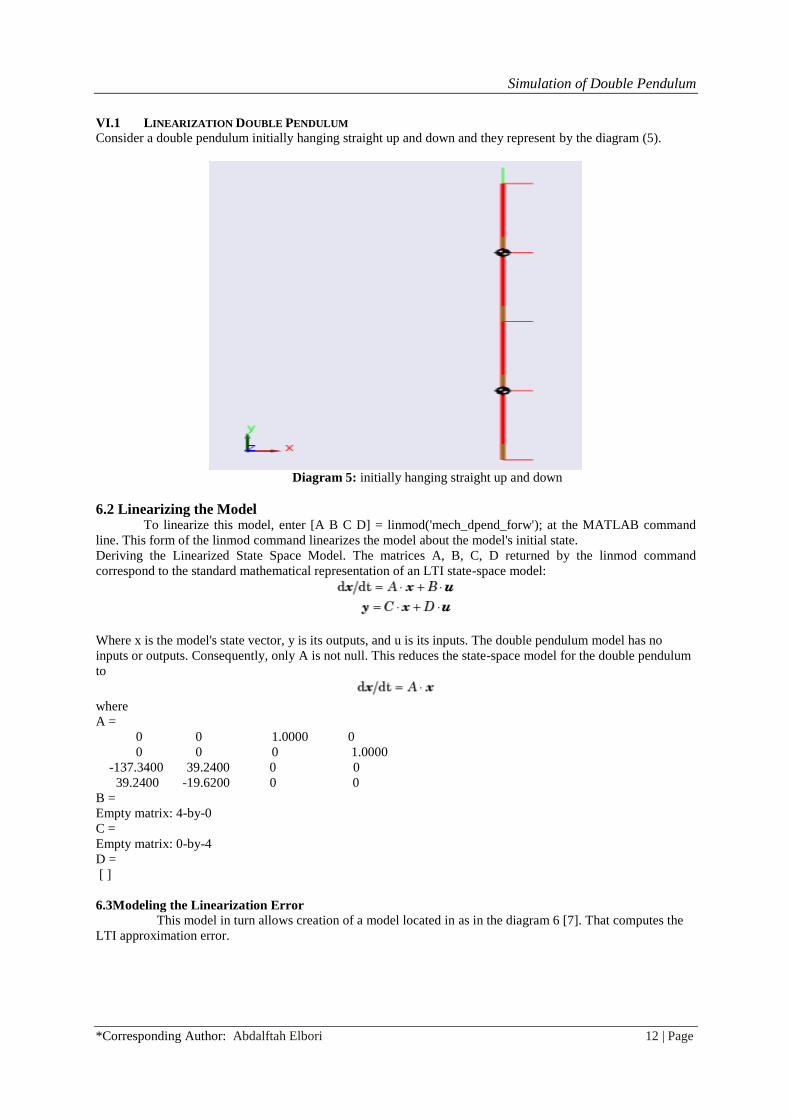
VI.1 LINEARIZATION DOUBLE PENDULUM Consider a double pendulum initially hanging straight up and down and they represent by the diagram (5).

Diagram 5: initially hanging straight up and down

6.2 Linearizing the Model To linearize this model, enter [A B C D] = linmod('mech_dpend_forw'); at the MATLAB command

line. This form of the linmod command linearizes the model about the model's initial state.

Deriving the Linearized State Space Model. The matrices A, B, C, D returned by the linmod command

correspond to the standard mathematical representation of an LTI state-space model:

Where x is the model's state vector, y is its outputs, and u is its inputs. The double pendulum model has no

inputs or outputs. Consequently, only A is not null. This reduces the state-space model for the double pendulum

to

where

A =

0 0 1.0000 0

0 0 0 1.0000

-137.3400 39.2400 0 0

39.2400 -19.6200 0 0

B =

Empty matrix: 4-by-0

C =

Empty matrix: 0-by-4

D =

[ ]

6.3Modeling the Linearization Error

This model in turn allows creation of a model located in as in the diagram 6 [7]. That computes the

LTI approximation error.



Location = [0 2 0]

Mass: 1 kg

Inertia: [0.083 0 0;0 .083 0; 0 0 0] kg.m2

CG: [0 1.5 0] (WORLD)

CS1: [0 0.5 0] (CG)

CS2: [0 -.5 0] (CG)

Mass: 1 kg

Inertia: [0.083 0 0;0 .083 0; 0 0 0] kg.m2

CG: [0 0.5 0] (WORLD)

CS1: [0 .5 0] (CG)

CS2: [0 -.5 0] (CG)

Position: 5 degrees

Velocity: 0 deg/s

Acceleration 0 deg/s/s

Position: 0 degrees

Velocity: 0 deg/s

Acceleration 0 deg/s/s

Ground

Upper Joint

Thin Rod

Thin Rod

Lower Joint

theta2

theta1

theta1

theta2

l inear

Scope

Env

B

F

J2

BF

J1

[theta2]

Goto1

[theta1]

Goto

G

[theta2]

From1

[theta1]

From

Error

CS

1C

S2

B1

CS

1

B

5

Diagram 6:

Running the model twice with the upper joint deflected 2 degrees and 5 degrees, respectively, shows an

increase in error as the initial state of the system strays from the pendulum's equilibrium position and as time

elapses. This is the expected behavior of a linear state-space approximation.

VII. CONCLUSION The Double pendulum is a very complex system. Due to the complexity of the system there are many

assumptions, if there was friction, and the system was non-conservative, the system would be chaotic. Chaos is a

state of apparent disorder and irregularity. Chaos over time is highly sensitive to starting conditions and can

only occur in non-conservative systems. The time of this motion is called the period, the period does not depend

on the mass of the double pendulum or on the size of the arcs through which they swing. Another factor

involved in the period of motion is, the acceleration due to gravity.

REFERENCES [1]. Kidd, R.B. and S.L. Fogg, A simple formula for the large-angle pendulum period. The Physics Teacher, 2002. 40(2): p. 81-83.

[2]. Kenison, M. and W. Singhose. Input shaper design for double-pendulum planar gantry cranes. in Control Applications, 1999.

Proceedings of the 1999 IEEE International Conference on. 1999. IEEE. [3]. Ganley, W., Simple pendulum approximation. American Journal of Physics, 1985. 53(1): p. 73-76.

[4]. Shinbrot, T., et al., Chaos in a double pendulum. American Journal of Physics, 1992. 60(6): p. 491-499.

[5]. von Herrath, F. and S. Mandell, The Double Pendulum Problem. 2000. [6]. Nunna, R. and A. Barnett, Numerical Analysis of the Dynamics of a Double Pendulum. 2009.

[7]. Callen, H.B., Thermodynamics and an Introduction to Thermostatistics. 1998, AAPT.

[8]. The Mathworks, 1994-2014 The MathWorks, Inc

[9]. http://www.mathworks.com/help/physmod/sm/ug/model-double-pendulum.html.

http://www.mathworks.com/help/physmod/sm/ug/model-double-pendulum.html

Documents

Research Paper Simulation of Double Pendulum · Simulation of Double Pendulum Abdalftah Elbori1, Ltfei Abdalsmd2 1(MODES Department, Atılım University Turkey)